Precipitation Distribution in Tropical Cyclones Using the Tropical Rainfall

Measuring Mission (TRMM) Microwave Imager: A Global Perspective

Manuel Lonfat1, Frank D. Marks, Jr.2, and Shuyi S. Chen1*

1Rosenstiel School of Marine and Atmosphere Science

University of Miami, Miami, Florida

2Hurricane Research Division

NOAA/AOML, Miami, Florida

Submitted to Monthly Weather Review

June 9, 2003

Revised

December 5, 2003

*Corresponding author address: Dr. Shuyi S. Chen, RSMAS/University of Miami, Miami, FL

33149. E-mail: schen@rsmas.miami.edu.

ABSTRACT

TRMM microwave imager rain estimates are used to quantify the spatial distribution of

rainfall in tropical cyclones (TC) over the global oceans. A total of 260 TCs were observed

worldwide from 1 January 1998-31 December 2000, providing 2121 instantaneous TC

precipitation observations. To examine the relationship between the storm intensity, its

geographical location, and the rainfall distribution, the dataset is stratified into three intensity

groups and six oceanic basins. The three intensity classes used in this study are: tropical storms

(TS) with winds < 33 m s-1, category 1-2 hurricane strength systems (CAT12) with winds from

34-48 m s-1, and category 3 to 5 systems (CAT35) with winds > 49 m s-1. The axisymmetric

component of the TC rainfall is represented by the radial distribution of the azimuthal mean

rainfall rates (R). The mean rainfall distribution is computed using 10 km annuli from the storm

center to 500 km radius. The azimuthal mean rain rates vary with storm intensity and from basin

to basin. The maximum R is about 12 mm h-1 for CAT35, but decreases to 7 mm h-1 for CAT12,

and to 3 mm h-1 for TS. The radius from storm center of the maximum rainfall decreases with

increasing storm intensity, from 50 km for TS to 35 km for CAT35 systems. The asymmetric

component is determined by the first-order Fourier decomposition in a coordinate system

relative to storm motion. The asymmetry in TC rainfall varies significantly with both storm

intensity and geographic locations. For the global average of all TCs, the maximum rainfall is

located in the front quadrants. The location of the maximum rainfall shifts from the front-left

quadrant for TS to the front-right for CAT35. The amplitude of the asymmetry varies with

intensity as well. TS shows a larger asymmetry than CAT12 and CAT35. These global TC

rainfall distributions and variability in various ocean basins should help to improve TC rainfall

forecasting worldwide.

1

1. Introduction

Predicting rainfall associated with tropical cyclones (TCs) is a major operational

challenge. Over the last few decades, fresh water flooding has become the largest threat to

human lives from TCs at landfall in the United States (Rappaport, 2000). While track forecasts

continue to improve, quantitative precipitation forecasts (QPF) for TCs have shown little skill.

One of the uncertainties in QPF is a lack of precipitation data over the open oceans to evaluate

and validate numerical weather prediction (NWP) model results. Early empirical TC rainfall

forecast models assume either a constant rain rate or axisymmetric rainfall distribution in TCs. A

number of case studies have shown that the precipitation structures in TCs are quite complex and

vary from case to case (e.g., Frank 1977, Miller 1958, Marks 1985, Burpee and Black 1989).

This study will provide a comprehensive analysis of the global TC rainfall characteristics using

TRMM observations. It is a critical step toward understanding and improving QPF in TCs.

Early radar images revealed that the TC rainfall is usually organized in bands spiraling

toward the storm center (Wexler 1947), commonly referred to as rainbands. A ring of intense

rainfall surrounds the storm center (e.g., Kessler 1954, Jordan 1960), known as the eyewall. The

spatial distribution of TC rainfall can be thought of as a series of annular means composed of an

azimuthal mean (or axisymmetric) and a perturbation (or asymmetric) component. Miller (1958)

made a composite of rain gage data from 16 hurricanes over Florida in a 3o array aligned with the

TC track. He observed a mean rain rate of 6.6 mm h-1 in the 1o box directly surrounding the

storm center. The mean rain rate in the remaining outer domain was 3.2 mm h-1. Rodgers and

Adler (1981) constructed radial profiles of rainfall for 21 eastern and western Pacific cyclones

using satellite passive microwave imager observations. They found that TC intensification was

accompanied not only by increases in the average rain rate, but also in the relative contribution

2

of the heavy rainfall. They also found that the radius of maximum rainfall decreased with

increasing storm intensity. Using airborne radar measurements Marks (1985) found the

azimuthal mean rain rate up to 11 mm h-1 in the eyewall of Hurricane Allen (1980), which was

about six times of that from the eyewall to 111 km radius. Burpee and Black (1989) examined

the radar-derived rainfall structure within 75 km of the center of Hurricanes Alicia (1983) and

Elena (1985). They found that the azimuthal mean rain rates in the eyewall were only 5.2 and 6

mm h-1, respectively. It dropped to 2.8 and 3.4 mm h-1 in the first rainband around the storm

center. These studies also showed that each storm has very different rainfall distributions during

its evolution, suggesting that many factors, both related to the storm dynamics and to its

environment, can influence the rainfall structure.

Asymmetries in the TC rainfall have been studied both observationally and numerically.

Radar observations showed rainfall asymmetry in Hurricanes Allen (Marks 1985), Alicia, and

Elena (Burpee and Black 1989). However, the asymmetry varies significantly from storm to

storm. Hurricane Allen had a rain rate maximum in the front-right quadrant in the eyewall region

shifted anticyclonically in the outer region. The rainfall maximum in Hurricane Alicia was first

observed in, which the front-left quadrant and later changed to the front-right quadrant. Other

observations have showed mixed results. Miller (1958) showed a maximum rainfall in the front-

right quadrant from the 16-storm composite for Florida. Frank (1977) found that rainfall

distributions were mainly axisymmetric for western North Pacific storms, using a 21-year record

of rain gages on 13 small islands. Using satellite observations, Rodgers et al. (1994) showed a

front maximum in a North Atlantic TC composite. The location of the maximum shifted to the

front-right as the storm translation speed increases. Although most previous studies found a

precipitation maximum ahead of the storm center, the variability in the location and amplitude is

3

large. In fact, storms with very similar locations, intensity, and speed, such as Hurricanes Allen,

Alicia, and Elena, can have very different rainfall structures.

The TC rainfall distribution is determined by many factors, including, but not limited to

environmental factors such as wind shear, sea surface temperatures (SST), and moisture

distribution, and TC-specific factors such as intensity, location, and translation speed. To

examine how these factors affect the TC rainfall, a quantitative description of the rain variability

is needed as a function of radius and azimuth around the storm center for various TC intensities,

locations and translation speeds.

In this study, the TRMM microwave imager rainfall product from 1998 to 2000 is used to

determine TC rainfall distributions over the global tropical oceans. Rainfall distributions for the

whole database separated by radius and azimuth for various TC intensity, location, and speed are

discussed.

2. Data and Analysis Method

a. TRMM data

TRMM is a joint mission between the U. S. National Aeronautics and Space

Administration (NASA) and the Japanese National Space Development Agency (NASDA). The

goal of TRMM is to measure global tropical rainfall (Simpson et al. 1988). The main instruments

onboard TRMM are a microwave imager (TMI), precipitation radar (PR), and a visible and

infrared radiometer system (VIRS). The TRMM satellite was launched in November 1997.

Before August 2001, it orbited at a 35o inclination and an altitude of 350 km. The satellite

altitude was then increased to 402 km to extend the mission lifetime. The potential of the satellite

resides in its ability to access both passive and active radiometric information. The 35o

4

inclination and TRMM’s non-sun synchronous orbit makes it an ideal platform to study TCs.

Details of TRMM instruments are given in Kummerow et al. (1998).

The TMI surface rainfall estimates (Kummerow et al. 1996) are used in this study. The

TMI swath is 750 km wide and the footprint is an ellipse with nearly 4 and 6 km axes. The

TRMM orbits containing TCs are selected by matching the TRMM database to linearly

interpolated best track information globally. The interpolated file provides the TC location,

intensity, speed, and direction of motion every 10 seconds. The times are matched to those for

the TRMM orbits and the distance between the storm center and the TRMM satellite nadir is

computed. If the distance is smaller than 500 km, the satellite observation is used in the analysis.

A maximum radius of 500 km was used to insure the data coverage exceeded 20% of the total

area within each annuli. As will be illustrated later, the data coverage decreases rapidly beyond

500 km radius. Only observations over the ocean are considered as the TMI rain algorithm

underestimates light rain over land.

b. TMI global sampling

During the period of 1 January 1998-31 December 2000, 260 TCs were observed

globally, providing 2121 TRMM/TMI instantaneous observations (Fig. 1). In this study, tropical

storms (TS) are defined as systems with wind speed1 from 18-33 m s-1, category 1-2 (CAT12)

systems with wind between 34-48 m s-1, and category 3 to 5 (CAT35) systems with wind > 49 m

s-1. The database contains observations from tropical storm to category-5 hurricane intensity.

Approximately 64% (1361) of the 2121 events are TS, 26% (548) are CAT12 and 10% (212) are

CAT35 systems.

1 The 6-h best track peak wind speeds interpolated to the TRMM orbit time are used to determine the storm intensity. In most basins, the peak wind speed is estimated from the 10-minute mean wind, whereas in the ECPAC and ATL basins it is the 1-minute sustained wind.

5

The observations are distributed among all TC basins around the globe. Six basins are

considered: Atlantic (ATL), East-Central Pacific (ECPAC), North West Pacific (NWPAC),

North Indian Ocean (NIND), South Indian Ocean (SIND), and South Pacific (SPAC). The

boundaries between basins are shown in Fig. 1. In order to determine if the TRMM dataset is

representative of the distribution of TCs over the 3-year period, the global TC distribution

observed by TRMM was compared to the best track record. Table 1 shows the percentage of all

observations and best track information in each intensity and basin group.

The best track and TRMM distributions are similar for most categories of Table 1. The

TRMM dataset is slightly biased toward strong storms in the Atlantic, as 50% of TRMM

observations are for hurricanes compared to 48.5% of the best track records. The combined

TRMM and the best track CAT12 and CAT35 frequencies are much higher in ATL than the

global average on the 1998-2000 period. All other basins, except NIND, show a combined

CAT12 and CAT35 percentage below the global average. The large number of CAT12 and

CAT35 observations in the Atlantic can be explained by the cold phase of ENSO for the period

sampled, during which more intense storms are expected in the Atlantic (Gray 1984, Shapiro

1987). During 1998, ENSO shifted from a cold to a neutral phase in which it remained through

the sampled period. NIND shows the largest discrepancy between the satellite database and the

best track distribution, as 36% of all SIND TRMM observations correspond to hurricanes, while

the best track states that only 26% were for CAT12 or higher. Finally, TRMM’s sampling of the

NWPAC is biased toward high TC intensity, compared to the three-year best track record

average by 3.5%. In summary, the TRMM/TMI dataset is representative of the global TC

activity from 1998 to 2000. The rainfall structure that will be discussed later should represent the

global TC rainfall well during a rather cold phase of ENSO.

6

c. Analysis methods

The rainfall characteristics are derived in storm relative coordinates. The radial variation

of precipitation is depicted by the azimuthal mean rain rate in 10 km wide annuli around the

storm center outward to the 500 km radius (Fig. 2). The resulting database allows us to compute

the radial dependence of the rain characteristics as a function of the storm intensity, location, and

speed.

Most instantaneous observations capture only part of the storm, because 1) the passive

microwave swath width is smaller than the size of most storms, and 2) the storm eye and satellite

nadir are rarely superimposed. Figure 3 shows the data coverage as a function of radial distance

from the TC center, normalized to the maximum possible coverage at all radial distances. The

coverage distribution in Fig. 3 is obtained by summing the area for each rain estimate (~25 km2)

in 10 km annuli around the TC center. These values are then compared to the area of each

annulus multiplied by the number of storm events observed by the satellite. For example, for all

2121 events, 8982 rain estimates of the inner 10 km annulus were obtained. The cumulative for

those estimates is 2.25x105 km2. The area of the inner 10 km ring is 314 km2, yielding a

maximum possible cover of 6.7x105 km2 for the 2121 overpasses. Hence, the ratio between the

actual and the ideal coverage is 33.7%. As seen in Fig. 3, the coverage is maintained between 30-

35% out to 200 km, and decreases linearly with radius beyond 200 km. At radii > 500 km, the

coverage decreases sharply below 20% and is therefore not considered in the analysis. Figure 3

also shows that similar results are obtained for the intensity subsets.

The probability density functions (PDFs) of rain rate occurrence (area) with radial

distance can also be determined using the annular database. The PDF is constructed by

classifying the TMI rain estimates, for each annulus, in a dBR scale, where

7

dBR=10Log10(R). (1)

The PDF is constructed for each annulus within 500 km radius by summing the occurrence of

rain estimates in each dBR class. Using the annular PDFs, a contoured frequency by radial

distance (CFRD) diagram can be constructed as a function of storm intensity, location, and

speed. PDFs and CFRDs provide information on the radial variability of the precipitation

distribution, and help to identify the median and mode of the rain rate distribution at any distance

from the center.

To examine the contribution to the total precipitation from various rain rates, PDFs and

CFRDs are also constructed for the total precipitation amount in each dBR class. The PDF is

obtained by weighing each rain estimate by the corresponding rain rate. The resulting

distribution is then normalized to the total amount of rain. This approach provides a PDF

distribution normalized by the total rain amount (flux) rather than by the total rain area. The

integral over the rain amount PDF divided by the integral over the occurrence PDF is the mean

rain rate of the raining area within the annulus. A median and a mode can also be defined for

each PDF of rainfall flux, yielding five measures of the rain distribution for each annulus. The

mean, median, and mode calculations in each PDF can yield very different values, particularly

when the PDF distribution is skewed. For TCs, the mode of the distribution is expected to shift

toward smaller rain rates as the distance from the center increases.

The next step of our analysis consists in studying the first-order asymmetry of the rain

distribution. The asymmetry is defined relative to the storm motion. The direction of the storm

motion at each TRMM observation is determined by linear interpolation of the two closest best

track reports to the observation time. As for the mean R computations, 10 km wide annuli around

the TC center are used to compute the spatial rainfall asymmetry. It is important to note that

8

missing data in the best track reduces the number of TRMM observations available for the

analysis. Nearly 80% of the initial TRMM observations can be assigned a storm direction.

In each annulus, the first-order Fourier coefficients are computed using all rain estimates:

a1= )cos([ iθ ]iiR∑ (2)

b1= )]sin([ iiiR θ∑ (3)

The spatial structure of the first-order asymmetry (M1) can be represented by:

M1 = Rba iiii/)]sin()cos([ 1 θθ +∑ (4)

where R is the mean rain rate calculated over the entire annulus (Boyd, 2001). The first-order

asymmetry is computed for different storm intensities, speeds, and locations.

d. Comparison of TRMM/TMI estimates with other datasets

The previous studies (e.g., Miller 1958, Frank 1977, Marks 1985, Burpee and Black

1989) that discussed the frequency distribution of rainfall in TCs can be used to estimate the

quality of the TRMM/TMI rainfall observations. Table 4 shows the rain rate stratifications

previous authors have used to construct the PDF. Examination of Table 4 shows that the TRMM

frequency distributions are similar to those from previous studies, both for the total storm PDF

and for the eyewall PDF. Rates < 0.25 mm h-1 are much less frequent in the TRMM PDF, and

rates between 0.25 and 6.25 mm h-1 occur more often. Consequently, TRMM redistributes very

low rates among the surrounding rainfall bins. As a result, the mean distributions will not be

affected except in the area where many 1-2.5 mm h-1 rates are observed. However, it likely will

not impact the mean rainfall. As Fig. 3 shows, only 24, 29 and 33% of the total area within 500

km of TS, CAT12 and CAT35, respectively is raining, and therefore zeros weigh heavily in the

mean calculation. TRMM/TMI estimates become particularly powerful in the asymmetry

9

analysis, which is a normalized calculation with accuracy strongly depending on the size of the

dataset.

The differences between TMI and other instruments may also illustrate the difficulties in

comparing PDFs of instruments with a wide range of resolutions. Miller (1958) and Frank (1977)

results are based on rain gage networks. Their datasets were large, but gages only offer point

measurements with 1-h accumulation and sampling area (~ a few km2) three orders of magnitude

smaller than that for TMI (~25 km2). The comparisons with the PDF of radar estimates are better

than those from the gages. Typical sampling area of ground and airborne radars are around 16

km2, which is closer to the TRMM/TMI sampling area.

3. Hurricane Dennis (1999)

The analysis methods described in section 2 are illustrated using a TRMM observation of

Hurricane Dennis on 29 August 1999. At 1800 UTC on 29 August, Dennis was off the coast of

northeastern Florida, at approximately 78.4oW and 30.8oN. The minimum sea level pressure

(MSLP) was near 970 hPa and the maximum sustained winds were about 50 m s-1, making

Dennis a category 3 hurricane. Dennis was moving almost due north at 5 m s-1. Dennis’ rainfall

displayed strong azimuthal variability in rainfall rates (Fig. 4). The rain is mostly on the left and

front-left of the storm center in the inner 150 km. In the outer region, the rainfall is mainly

located in a strong rainband on the front and front-right of the storm center.

Figure 5 shows the azimuthal mean rain rates as a function of the radial distance from the

storm center in Hurricane Dennis. The peak rainfall is located 60 km from the center and is about

13.5 mm h-1. Several secondary peaks in rainfall can be seen at 150 km and 275 km radii,

corresponding to a broad zone of precipitation in the front-left quadrant of the storm, and a more

intense but narrower region farther to the front-right quadrant of the storm (Fig. 4). The eyewall

10

is well defined in the precipitation distribution, at 60 km from the center. The eye is not totally

clear of rain.

The PDF of rain occurrence for the entire storm is shown in Fig. 6. Rain rates are

between 0.4 and 40 mm h-1. Most of the rainfall area (~91%) within 500 km of Dennis’ center

falls between 1 and 10 mm h-1. It is important to note that rainfall covers only 25% of the total

area within 500 km of the storm center. The mode is at 7 mm h-1. The distribution also shows a

secondary maximum near 1.5 mm h-1. The stratiform rain area in the rainbands contributed the

most to the 7 mm h-1 peak. The 1-2 mm h-1 rainfall mostly occurs between the eyewall and

rainbands. The total distribution in Fig. 6 is skewed toward higher rates, which shows that

convective type rainfall from the eyewall and rainband dominates the distribution. The change in

the PDF of rain occurrence as a function of the radial distance to the storm center is shown in

Fig. 7. Within the inner 50 km radius, the mode sharply increases with distance to reach 10 mm

h-1 at the 50 km radius. Between 50 and 75 km, the distribution broadens because of the rainfall

asymmetry present in Dennis’ eyewall (Fig. 4). Between 75 and 200 km, the mode decreases

with distance, from approximately 10 mm h-1 to 4 mm h-1. The distribution narrows as the storm

shows a more horizontally uniform rain pattern. Further out, the distribution broadens again and

the mode increases, due to the presence of the right-front rainband. In general, the width of the

PDF provides good indications of the degree of symmetry of the storm rainfall. Dennis’ PDF

illustrates that even at large distances (> 300 km), high rainfall rates (> 40 mm h-1) can be

observed, although the probability is only a few percent.

Figure 8 shows the rainfall flux PDF with radial distance for Hurricane Dennis.

Compared to the PDF of rain occurrence (Fig. 7), both the mode and median of the distribution

in Fig. 8 occur at higher rain rates, although differences between the modes of both figures are

11

small. The rainfall flux distribution is heavily influenced by large rates, which is shown by the

large shift in the median from the PDF of occurrence to the rainfall flux PDF. The shift toward

higher rates is more pronounced for the median than for the mode, particularly in the eyewall and

rainband areas. In these two areas, most of the rain flux can be attributed to rainfall rates > 3-4

mm h-1. Those two regions are also the areas with the largest asymmetries, where rates > 20 mm

h-1 were observed. The medians for both distributions were very similar in the region between 75

and 250 km, where the storm was more symmetric.

To examine the asymmetry in the spatial distribution of rainfall, the first order Fourier

analysis of Dennis rainfall is computed relative to the storm motion, using equations (2)-(4). The

solid dots on top of the rainfall map in Fig. 4 show the general location of the first order

asymmetry phase maximum. The three dots corresponding to the inner three annuli (outward to

150 km) are located primarily on the left of the storm center, in agreement with the asymmetry in

the eyewall rainfall. The three dots corresponding to the annuli between 150 km and 300 km are

located in the front-right quadrant, where the rainband precipitation is observed. Figure 9 shows

the wavenumber 1 asymmetry spatial distribution within 300 km of Dennis’ center. Larger

asymmetries are observed at larger radii. Asymmetry amplitudes are much smaller near the

center, as the rainfall surrounds the entire storm eye. The amplitudes in Fig. 9 are normalized to

the ambient mean rainfall, so that the amplitude near unity ahead of the center at 275 km means

that the wavenumber 1 signal is as strong as the axisymmetric average. The various analyses

introduced in this example are applied to the extended three-year statistics in the next section.

4. Characteristics of the TC rainfall distribution

a. PDF of rain rates

12

Figure 10 shows the PDF distributions by area of occurrence for all TRMM rainfall

observations within an area of 500 km radius around the storm centers. The mode is near 0 dBR

(1 mm h-1), but not unique, as all distributions in Fig. 10 show a second maximum near 5 dBR

(3.2 mm h-1As the storm intensity increases, the median and the mode of the distribution shift

toward higher values and the distribution tends to become broader with increasing storm

intensity.

Similar characteristics are observed in the basin PDFs (Fig. 10c). The Atlantic basin

distribution is similar to the overall PDF for CAT12 and CAT35, which is not surprising as more

observations of hurricanes were obtained in the Atlantic than in other basins during the 1998 to

2000 period (Table 1). The ECPAC has the least total rain of all basins with a narrower

distribution and the largest percentage of TS observations (Table 1). In agreement with the

results of Fig. 10b, the ATL and ECPAC define the envelop for the remaining basin PDFs.

However, the trend in the remaining basins is not as clear, as illustrated by the NIND, SIND, and

SPAC PDFs. Those three basins show large differences in the modal frequency and amplitude of

the PDF, although distributions among intensities are very similar for each basin (Table 1).

Hence, the TC intensity is most likely not the most important factor explaining the PDF

distribution by occurrence.

b. Azimuthal averages

The radial distributions of azimuthally averaged rainfall rates for all observations and

each of the three storm intensity categories are shown in Fig. 11a. Rain rates up to 5 mm h-1 are

found within 50 km of the TC center for all observations. They decrease outward to 1 mm h-1 at

250 km. The maximum rain rate is located at 40 km from the storm center. Mean rain rates

increase with storm intensity at all radii. Peak mean rates are 3, 7, and 12.5 mm h-1 for TS,

13

CAT12 and CAT35 systems, respectively. The location of the peak rainfall also varies with

intensity, from about 50 km from the storm center for TS to 35 km for CAT35 systems. Marks

(1985), using a rainfall distribution from airborne radar observations for Hurricane Allen (1980),

showed a mean rain rate of 11.3 mm h-1 in the eyewall and 1.8 mm h-1 in the region extending

from the outer edge of the eyewall to a radius of 111 km. At the time of the measurements,

Allen’s minimum sea-level pressure (SLP) varied from 960 mb to 910 mb, making it an upper

CAT12 to CAT35 in our description. The radius of maximum wind in Allen fluctuated between

12 and 40 km. Assuming that the peak rain rates in the TRMM distribution can be identified with

the mean location of the eyewall, the peak rates observed with TRMM for CAT12 to CAT35

storms compare well with Marks’ (1985) findings.

In the TRMM statistics, the area extending from the eyewall (35-40 km) to the 111 km

radius yields 8.4 mm h-1 and 5.7 mm h-1 for CAT12 and CAT35 storms, respectively. These rates

are larger than those mentioned in Marks (1985). However, TRMM probably overestimates the

rain rates in the central dense cloud overcast (CDO) region (Lonfat et al., 2001). Rain rates in

Allen also decreased more sharply with radius compared to other observations by Burpee and

Black (1989). These authors also partitioned the observations into the eyewall and rainband

regions. Hurricane Alicia’s eyewall fluctuated between 20 and 35 km, while Hurricane Elena’s

eyewall remained at 35 km. The rainband region in Burpee and Black (1989) extended to 75 km,

instead of the 111 km as in Marks’ study. Both storms were classified as CAT12, with minimum

SLP near 960 mb. Rain rates of 5.2 and 6 mm h-1 in the eyewall and 2.8 and 3.4 mm h-1 in the

rainband were observed in Alicia and Elena, respectively. TRMM CAT12 mean rates in the

region extending from 35 km (eyewall) to 75 km were 7 and 6.4 mm h-1, respectively. The ratio

of eyewall to rainband rain rate was near 1.8 for both Alicia and Elena. The same ratio calculated

14

with TRMM was 1.1. Hence, the TRMM rates in the rainband region is high compared to that

from the radar studies.

Miller (1958) provides a comparison of rainfall in the outer region. The inner 1o box (~

60 km radius) and the average of the 8 surrounding 1o boxes (~ 200 km radius) yield 6.6 and 3.2

mm h-1 for the inner and outer regions, respectively. Using the TRMM CAT12 distribution with

60 and 200 km radii, the means are 6.7 and 3.9 mm h-1, respectively. Including a larger area in

the rainband mean calculation provides a better result, confirming that TRMM tends to

overestimate the rain in the region outside the eyewall.

Differences in the mean rain rates of various TC intensities occur almost exclusively

within 250 to 300 km of the storm center, which is partly associated with different relative

contribution of convective to stratiform precipitation at various intensities (Lonfat et al., 2001).

Furthermore, the frequency distribution of non-raining area with radius relative to the total area

also contribute to the variation (Fig. 12). Less than 5% of all observations are larger than 15 mm

h-1 at 250 km radius, which is true for all storm intensity groups. The non-raining area in Fig. 12

reaches 65% of the entire area within 250 km. The distributions of non-raining area with TC

intensity merge together by the 300 km radius. The decrease in heavy rain, combined with a

sharp increase in non-raining area, most likely explains the variability in the mean rainfall within

250 km of the center.

Figure 11b shows the azimuthal mean rain rates stratified by TC geographic location. The

variability in mean rainfall is large from basin to basin. The mean rain rates vary between 4 and

10 mm h-1 within the inner 50 km radius. The NIND basin TCs show larger rates than the other

basins within the inner 100 km radius. Although the remaining basin distributions look similar,

up to 50% differences in mean rates between basins are observed within the inner 250 to 300 km.

15

The ECPAC TCs rain less than other basins throughout most of the 350 km radius shown in Fig.

11b. Three possible scenarios may explain the basin variability: (a) biases in the TC intensity

sampling may artificially increase or decrease the true basin averages by altering the distribution

of observations among the different TC intensity classes in each basin; (b) the variability among

intensity classes may be responsible for the different basin distributions; and (c) differences in

the TC-environment interactions in each basin may alter the distribution associated with intensity

changes shown in Fig. 11a.

Our results do not support the first two scenarios. The variability observed in Fig. 11b

cannot be explained by a sampling problem. The TRMM observation distribution is

representative of the natural global distribution of TCs, as expressed by the best track

information in Table 1. However, the ATL basin showed similar mean rain estimates than other

basins, such as NWPAC, even though it had more observations of CAT12 and CAT35 than any

other basin between 1998 and 2000. Also, the two basins showing the largest rainfall rates

(NIND and SPAC) have only 26.3 and 30.5% of observations in the hurricane categories,

respectively. ECPAC and NWPAC have similar frequencies, although their mean R distributions

in Fig. 11b show smaller rates throughout the radial distribution. Consequently, the intensity

trend shown in Fig. 11a does not apply to all basins. Hence, the way intensity and rainfall

correlate in each basin must depend on the state of the environment and ocean-atmosphere

boundary layers, suggesting (c) is most likely the scenario. The intensity trends in each basin

need to be computed to confirm this assumption. However, the current database, described in

Table 1, is not large enough to provide significant results in all basins for CAT12 and CAT35.

c. Rain rate probability with radial distance

16

Figures 13 and 14 show how the CFRDs by area of occurrence evolve with radial

distance to the TC center. The CFRDs are computed outward to 500 km radius of the TC center.

Figure 13 shows the CFRD by area for all 2121 observations. The mode decreases from 4 mm h-1

in the inner 50 km to 1 mm h-1 by the 200 km radius. At ranges > 200 km, the peak remains at 0

dBR.

An important property of the TC rainfall distribution that the PDF does not account for is

the frequency of occurrence of non-raining observations. The non-raining area is expected to

increase with radial distance, as the area itself increases with the square of the radius. The solid

curve in Figure 12 shows the radial distribution of non-raining observations. The values are the

frequencies of zero rain observations relative to the total number of observations at any distance

from the TC center. Inferring that those values represent the storm non-raining area assumes that

our sampling of rain and no-rain areas is uniform, as TRMM does not observe the entire storm

area. This assumption is most likely legitimate, as the total number of TRMM observations

obtained in each quadrant of the storm is similar.

Several interesting features are noticeable in Fig. 12. The non-raining frequency increases

with distance outward of 50-100 km radius. A frequency minimum is observed near 50 km

radius (typical radius of maximum rain). Frequencies increase in the inner 30 to 50 km. The

inner 50 km increase in frequencies indicates the presence of the eye. The frequency minimum

corresponds to the mean location of the eyewall, and the trend of increasing frequencies with

radial distance corresponds to the increase in area that is not matched by the rainfall contribution

as the radius increases.

Figure 14 shows the CFRD distributions by area grouped by storm intensity. The

distributions vary with intensity within the 250-300 km radius of the storm center. In that region,

17

the mode increases with intensity. TS have a broader distribution than CAT12 and CAT35 in the

inner 250 km. Assuming that the width of the distribution is a measure of the asymmetric nature

of the TCs, TS seem more asymmetric in the inner core. In the region beyond 250 km, the

CFRDs of CAT12 and CAT35 broaden, indicating an increase in the asymmetry amplitude. In

the outer area (range>250 km), the mode is found at 1 mm h-1, uniformly through all PDFs. The

CFRDs in Figs. 13 and 14 show that at radii > 250 km, for all intensities, rain rates >40 mm h-1

can still be observed with a probability of a few percent.

The general features of the no-rain distribution hold true when the data is partitioned with

storm intensity. A strong variability in the no-rain frequencies exists within the inner 350 km of

the TC (Fig. 12). Nearly half of all observations in the inner 150 km of TS are non-raining, while

90% of observations correspond to rain in the same area for CAT35. The inner 150 km region of

CAT12 shows 20-30% non-raining area. There is a distinct change in distributions from TS to

CAT12 and CAT35. This change is most likely associated with the dynamic structure of the

storm. As the intensity increases, the transport of rainfall by the swirling winds may more

efficiently redistribute the rainfall around the entire storm. Rain that may be produced locally in

convective cores is going to spread over greater areas as the wind increases (e.g., Marks and

Houze 1987). The number of convective cores may increase in the stronger systems. At large

radii, the distributions of non-raining observations as a function of intensity all merge and the

non-raining area does not increase geometrically, which means that the area where rainfall

occurs increases with radial distance.

The relative contribution of each rain rate to the total volume (flux) of precipitation is

shown in Figs. 15 and 16. Figure 15 shows the CFRD of flux for all 2121 TC events. The inner

core mode is at 30 mm h-1 and extends to the 50 km radius. A second mode, at 11 mm h-1,

18

extends from 40 to about 240 km. At large distances, the mode shifts toward 3 mm h-1. The step-

like mode structure with radial distance is also observed when the observations are stratified by

intensity. The modes are found at similar rain rates at all intensities, but their amplitudes vary

with the storm strength. As the storm becomes more intense, the width of the PDF narrows, so

that the mode frequency increases. This trend holds particularly well within the inner 300 km. At

further distances, the PDFs look very similar, taking into account that the size of the dataset

reduces with TC intensity, which introduces some noise in the PDF. While the high rain rates (>

10 mm h-1) make up < 15% of the total inner core area, for all 2121 observations averaged

together, they contribute about 50% of the total rainfall. Similarly, Marks (1985) found that the

eyewall rainfall in Allen contributed to nearly 40% of the total amount within a radius of 1o

latitude from the storm center. All TMI distributions have an upper limit near 50 mm h-1. These

higher rates contribute less than 1% to the total volume of rainfall within the storm.

d. Rainfall asymmetry

Figure 17 shows the storm-motion-relative spatial distribution of rainfall asymmetry for

all observations globally (Fig. 17a) and for each intensity group (Figs. 17b-d), respectively. The

overall storm composite shows that M1 maximum is located in the front quadrants (Fig. 17a).

This asymmetry is similar for TS (Fig. 17b). However, as the storm intensity increases, the M1

maximum shifts from the front-left to the front-right quadrant. The shift suggests that the rainfall

asymmetry correlates with the asymmetry in the tangential wind circulation.

The asymmetries in CAT12 and CAT35 storms are consistent with those observed by

Burpee and Black (1989) and Marks (1985). Burpee and Black observed a strong wavenumber 1

in the composite rainfall structure of Hurricane Alicia. The maximum rainfall was observed in

the front-left quadrant and the minimum in the rear-right quadrant, for both the eyewall and the

19

rainband area within 75 km radius. In the eyewall, the maximum was 2.5 times larger than the

minimum. In Elena, Burpee and Black observed a rainfall maximum in the front-right of the

storm center. Elena had a stronger rainfall asymmetry than Alicia, with a maximum to minimum

ratio of seven. Marks found that a front-right maximum rainfall in the eyewall region of

Hurricane Allen. These features are similar to the observed patterns in Figs. 17c and d. As the

storm evolves, the asymmetry varied substantially with time. Burpee and Black noted a large

variability in the asymmetry of Hurricane Alicia. However, coastal influences may explain some

of the variability in their observations.

The differences in asymmetry amplitude among the various intensity groups are likely

related to the strength of the primary circulation of the vortex. TS have the largest asymmetry

throughout the 300 km area. The amplitudes reach 30% of the azimuthal mean rainfall at 300 km

in the front of the storm center. Although TS have a weaker and less organized circulation than

CAT12 and CAT35 storms, deep convection does not seem to be randomly distributed around

the storm center. Most TS are aggregates of mesoscale convective systems in the early stage of

their lifecycle. The rainfall maximum is in the front of the storm center (Fig. 17b), where the

friction induced asymmetry in the circulation of the moving storm may play an important role in

enhancing the deep convective activity by creating a low-level convergence anomaly ahead of

the storm. As the storm intensity increases, the primary circulation becomes stronger and more

symmetric (e.g., Marks and Houze 1987, Croxford and Barnes 2002) (Fig. 17d). This simple

picture does not take into account the various possible physical processes that may affect the TC

rainfall asymmetry, as will be discussed in the next section.

Figure 18 shows the TC rainfall asymmetry as a function of the geographic locations. In

all basins, the M1 maximum is located in the front quadrants. However, large differences in

20

rainfall asymmetry are also evident among different basins. There are significant differences

between the Northern and Southern Hemisphere asymmetry distributions. TCs in the Southern

Hemisphere have a clear M1 maximum in the front-left quadrant (Figs. 18d and f). In the

Northern Hemisphere, M1 peaks in the front-right quadrant. This is particularly evident in the

Atlantic basin (Fig. 18a). It is interesting that M1 maximum shifts cyclonically from the center

outward in both the East-Central Pacific basin and the North Indian Ocean Basin (Figs. 18b and

e), whereas it is shifted anticyclonically and much weaker in the NWPAC. The M1 maximum in

Atlantic TCs remains in the front-right quadrant from the center out to 300 km, which is in

agreement the location of maximum lightning occurrence in Atlantic hurricanes found by with

Corbosiero and Molinari (2003). The first-order asymmetry amplitudes increase outward from

the center in all basins. TCs in NWPAC and SPAC basins (Figs. 18c and d) have the smallest

asymmetry, whereas the Indian Ocean TCs (Figs. 18e and f) have the largest.

5. Factors affecting rainfall asymmetry

Several factors are known to affect TC rainfall asymmetry, such as advection of planetary

vorticity, vertical wind shear (e.g., Rogers et al 2003) and friction-induced convergence in the

boundary layer (e.g., Marks 1985). The differences in rainfall asymmetry observed between the

Northern and Southern Hemispheres (Fig. 18) seem to indicate advection of planetary vorticity

plays a critical role, particularly in weak TCs. The amplitude of rainfall asymmetry is small in

hurricanes (less than 15% of the ambient mean rain amount within the inner 300 km). The

distinct patterns of rainfall asymmetry for different ocean basins (Fig. 18) seem to indicate the

friction induced by low-level convergence and vertical wind shear must play a role as well.

However, it is difficult to examine the complex effects of vertical wind shear without a good

21

global wind dataset. Hence, the following discussion focuses on the effects of boundary layer

convergence on the observed rainfall asymmetry.

The importance of the TC motion on rainfall asymmetries is investigated by dividing the

dataset into two groups: fast (> 5 m s-1) and slow (< 5 m s-1) moving TCs. Figure 19 shows the

spatial distribution of M1 for the two groups. There is no significant difference in M1 pattern for

the slow and fast moving TCs, except the amplitude is larger for the fast moving TCs. The M1

maximum is ahead of the storm center for both groups, consistent with the overall TC asymmetry

shown in Fig. 17a. However, the amplitude of M1 varies with the speed of the storms at large

radii (Fig. 19). At 275 km from the storm center, faster TCs have amplitudes as large as 50% of

the ambient mean rain rate, while the amplitudes for the slower TCs do not reach 20% of the

ambient value. Shapiro (1983) studied the effect of the storm motion on the boundary layer of a

hurricane inner core (within approximately half a degree radius). A convergence anomaly was

observed in front of the storm, resulting in enhanced rainfall ahead of the storm center. The

anomaly shifted from the front to the front-right quadrant with increasing storm speed.

Hurricanes Alicia and Elena (Burpee and Black 1989) were slow movers. Alicia’s speed

increased from 1.5 to 2.3 m s-1 during the period of observation. The maximum rainfall shifted

from the left to slightly right of the track with increasing speed. The asymmetry amplitude

remained similar. Hurricane Elena, slightly faster at 5 m s-1, had maximum rainfall in the front-

right quadrant. However, the asymmetry amplitude in Elena was twice as large as in Alicia.

Although Hurricane Allen was moving much faster than Alicia and Elena, at 10 m s-1, its

asymmetry location and amplitude were comparable to that in Elena. This complexity is closely

related to the storm environmental conditions as well as storm-environment interactions, which

are not well understood.

22

Each intensity and oceanic basin group can be further divided into the two speed

categories defined above. The number of TCs with translation speed < 5 m s-1 is about 60% for

TS, 48.5% for CAT12, and 56.6% for CAT35, respectively. These numbers do not vary much

with storm intensity, although CAT12 storms are slower on average than other groups. However,

the TC translation speed varies significantly from basin to basin. 43% of ATL storms were slow

movers, compared to 50.5% in ECPAC, 56% in NWPAC, 76.8% in NIND, 74.9% in SPAC, and

60.8% in SIND systems. TCs in the Indian Ocean basins and the South Pacific are slow movers,

while the Atlantic storms are the fastest on average. If the variability in translation speed can

explain the rainfall asymmetry, one would expect the Atlantic storms to show the largest

asymmetry amplitudes, while the Indian Ocean and South Pacific storms should be more

symmetric. Results shown in Fig. 18 do not confirm this. Hence, other mechanisms, such as the

vertical wind shear must play at least a as important role as the translation speed on TC rainfall

distributions.

6. Conclusions

Precipitation distributions in TCs have been studied globally using observations from the

TRMM TMI. Between 1 January 1998 and 31 December 2000, 2121 instantaneous

measurements were collected in 260 TCs with intensity ranging from tropical storm to category 5

hurricane and located in all oceanic basins. The spatial distribution of rainfall was partitioned

into an azimuthal average and a wavenumber 1 asymmetry. PDFs are constructed as a function

of TC intensity and geographic location.

The PDF analysis was used for comparison of TRMM distributions with previous studies.

TRMM/TMI PDF captures the general features described by previous studies. TMI

underestimates the small rates (<0.25 mm h-1), which is probably due to the instrument

23

resolution. The frequency for rain rates < 2.5 mm h-1 is too high, which indicates that the TMI

algorithm may redistribute the lowest rates to the adjacent rainfall bins. This problem does not

bias our analysis, except in a region extending between 100 and 250 km, where the 1 to 2.5 mm

h-1 rates are most prevalent. The asymmetry analysis is independent of the absolute values of the

estimates, because the quadrant rates are normalized to the ambient azimuthal mean rates. The

maximum rate observed by TRMM/TMI is ~50 mm h-1, with a frequency of ~1%. More

generally, the heavy rainfall (R>10 mm h-1) covers only 15% of the inner core area, but

contributes 50% of the total rainfall amount.

The location of the peak azimuthal mean rain rate shifts to a smaller radius when the TC

intensity increases, similar to the observation of Rodgers and Adler (1981) and Marks (1985).

The Indian Ocean storms show the largest azimuthal mean rain rates of all basin distributions.

Atlantic and West Pacific storms have very similar mean distributions. East-central Pacific

storms show the smallest mean rates, possibly because of the cooler SST conditions prevailing in

the Eastern Pacific region. However, the intensity relationship deduced for the total database

does not apply in each basin. Consequently, how the storm intensity and the rainfall distribution

relate to each other depends on the environmental conditions, specific to each basin.

The wavenumber 1 asymmetry in TC rainfall is found to shift from the front-left to the

front-right quadrant with increasing intensity. The tropical storms show the largest asymmetries.

Hurricane strength storms tend to have a more axisymmetric inner core. In all basins, the

asymmetry remains in the front quadrants. The storm location is an important factor, as southern

hemisphere storms show asymmetry to the left of the storm track, while north hemisphere

cyclones rainfall peaks in the front-right quadrant. The storm translation speed also plays an

important role in the rainfall asymmetries. The rainfall maximum is located in front of the storm

24

center at all speeds, but its amplitude increases with speed. Consequently, frictional convergence,

as mentioned by Shapiro (1983), most likely plays an important role on the rainfall structure.

However, the basin to basin variability in storm motion is not reflected totally in that for the

rainfall asymmetry. Hence, other mechanisms, such as the vertical shear may play an important

role on the rainfall distributions.

The next step in the analysis will be to study the asymmetries in a shear-relative

coordinate system, instead of in the motion-relative coordinate system. Rogers et al. (2003)

derived a relationship between the track-relative location of the accumulated rainfall and the

direction of the vertical shear vector relative to the storm direction using MM5 simulations of

Hurricane Bonnie. The total precipitation showed strong sensitivity to the shear direction and

amplitude. The rainfall was found to accumulate down-shear left, so that depending on the

direction of motion, relative to the orientation of the shear, the spatial distribution of total rainfall

along the track could be either symmetric or strongly asymmetric. TRMM, alongside global

wind data, can provide statistical information regarding the effect of shear on the instantaneous

precipitation distribution. However, the relative contribution of the shear effect with respect to

other processes such as frictional convergence or the β-effect mechanism is still not clear. Using

TRMM, a detailed diagnostic study of the relative contribution of all processes can be

constructed globally. Storm simulations, along with the results described here, will allow

improvements of our knowledge of the precipitation structure of tropical cyclones and of the

dynamics governing the rainfall structure. Our study can be used as a climatologic basis toward

improving the current forecasting techniques. The mean distribution can help correct simple

rules of thumb, still a common practice today. Including the asymmetry analysis will also refine

25

further current techniques, as most often the precipitation structure shows at least some degree of

asymmetry.

Acknowledgements. The first author is supported by the NASA Earth Science System

Fellowship (NGT5-30425). We thank Dr. Jeffrey Hawkins and two anonymous reviewers for

their helpful comments and suggestions. This work is partially supported by a NASA grant

NAG5-10963 and a NSF grant ATM9908944.

26

References

Boyd, J. P., 2001: Chebyshev and Fourier spectral methods. Second Edition, p. 44, Dover

publications, Inc., New York.

Burpee, R.W. and M. L. Black, 1989: Temporal and spatial variations of rainfall near the centers

of two tropical cyclones. Mon. Wea. Rev., 117, 2204-2218.

Corbosiero, K. L. and J. Molinari, 2003: The relationship between storm motion, vertical wind

shear, and convective asymmetries in tropical cyclones. J. Atmos. Sci., 60, 366-376.

Croxford, M. and G. M. Barnes, 2002: Inner core strength of Atlantic tropical cyclones. Mon.

Wea. Rev., 130, 127-139.

Frank, W. M., 1977: The structure and energetics of the tropical cyclone. Part I: Storm structure.

Mon. Wea. Rev., 105, 1119-1135.

Gray, W. M., 1984: Atlantic seasonal hurricane frequency, part I: El Nino and 30 mb quasi-

biennial

oscillation influences. Mon. Wea. Rev., 112, 1649-1668.

Jordan, C. L., D. A. Hurt, and C. A. Lowrey, 1960: On the structure of hurricane Daisy on 27

August 1958. J. Meteor., 17, 337-348.

Kessler, E., 1954: Eye-region of Hurricane Edna, 1954. J. Meteor., 15, 264-270.

Kummerow, C., W. S. Olson, and L. Giglio, 1996: A simplified scheme for obtaining

precipitation and vertical hydrometeor profiles from passive microwave sensors. IEEE

Trans. Geosci. Remote Sens., 34, 1213-1232.

Kummerow, C., W. Barnes, T. Kozu, J. Shiue, and J. Simpson, 1998: The tropical rainfall

measuring mission (TRMM) sensor package. J. Atmos. Oc. Tech., 15, 809-817.

27

Lonfat, M., F. D. Marks, Jr., and S. S. Chen, 2001: Comparison of TRMM TMI-PR and

Airborne Radar Data for Four Major Atlantic Hurricanes. AGU General Assembly, San

Francisco, December 2001.

Marks, F. D., Jr., 1985: Evolution of the structure of precipitation in Hurricane Allen (1980).

Mon. Wea. Rev., 113, 909-930.

Marks, F. D., Jr., and R. A. Houze, Jr., 1987: Inner Core Structure of Hurricane Alicia from

Airborne Doppler Radar Observations. J. Atmos. Sci., 44, 1296-1317.

Miller, B. I., 1958: Rainfall rates in Florida hurricanes. Mon. Wea. Rev., 7, 258-264.

Rappaport, E. N., 2000: Loss of life in the United States associated with recent Atlantic tropical

cyclones. Bull. Am. Met. Soc., 81, 2065-2074.

Rodgers, E. B. and R. F. Adler, 1981: Tropical cyclone rainfall characteristics as determined

from a satellite passive microwave radiometer. Mon. Wea. Rev., 109, 506-521.

Rodgers, E. B., S. Chang, and H. F. Pierce, 1994: A satellite observational and numerical study

of precipitation characteristics in Western North Atlantic tropical cyclones. J. Appl.

Meteor., 33, 129-139.

Rogers, R., S. S. Chen, J. Tenerelli, and H. Willoughby, 2003: A numerical study of the impact

of the vertical shear on the distribution of rainfall in Hurricane Bonnie (1998). Mon. Wea.

Rev., in press.

Shapiro, L. J., 1983: The asymmetric boundary layer flow under a translating hurricane. J.

Atmos. Sci., 40, 1984-1998.

Shapiro, L. J., 1987: Month-to-month variability of the Atlantic tropical circulation and its

relationship to tropical storm formation. Mon. Wea. Rev., 115, 1598-1614.

28

Simpson, J., R. F. Adler, and G. R. North, 1988: Proposed tropical rainfall measuring mission

(TRMM) satellite. Bull. Am. Met. Soc., 69, 278-295.

Wexler, H., 1947: Structure of hurricanes as determined by radar. J. Atmos. Sci., 48, 821-844.

29

Tables

Table 1: Comparison of TRMM TC observations and 6-hourly advisory distributions with

the cyclone intensity, in each oceanic basin.

Table 2: Comparison of TRMM rainfall PDFs with previous studies. The rainfall is

partitioned into rate intervals (bins) used in previous studies.

30

Table 1. Comparison of TRMM TC observations and 6-hourly advisory distributions with the cyclone intensity, in each oceanic basin.

TS CAT12 CAT35 Total

Basin TRMM Best

track

TRMM Best

track

TRMM Best

track

TRMM Best

track

ATL 238 (50) 651

(54.5)

178

(37.5)

385

(32)

60

(12.5)

162

(13.5)

476

(22.5)

1198

(21.5)

ECPAC 234 (69) 880

(68)

74 (22) 280

(22)

31 (9) 132

(10)

339 (16) 1292

(23)

NWPAC 455

(67.5)

1128

(71)

168 (25) 331

(21)

52 (7.5) 124 (8) 675 (32) 1576

(28)

NIND 46 (64) 177

(74)

17

(23.5)

40

(16.5)

9 (12.5) 23 (9.5) 72 (3.5) 240

(4.5)

SIND 168 (70) 329

(75.5)

50 (21) 69 (16) 21 (9) 37 (8.5) 239 (11) 435

(7.5)

SPAC 220 (69) 609

(69.5)

61 (19) 174

(20)

39 (12) 94

(10.5)

320 (15) 877

(15.5)

Total 1361

(64)

3774

(67)

548 (26) 1279

(23)

212

(10)

572

(10)

2121 5625

31

Table 2. Comparison of TRMM rainfall PDFs with previous studies.

Rain threshold (mm h-1) <0.25 0.25-6.25 6.25-19 >19

Miller (1958) 1o box 32 47 17 4

Frank (1977) 2o box 30 54 13 3

Marks (1985) 111km radius 23 69 6 2

TRMM- 111 km radius 0.5 74 21 4.5

TRMM- 222 km radius 1 81 16 2

TRMM- 500 km radius 1 84 13 2

Rain threshold (mm h-1) <2.5 2.5-5 5-10 10-25 >25

Burpee and Black (1989) Eyewall-Alicia 59 13 12 12 4

Burpee and Black (1989) Eyewall-Elena 58 13 12 11 6

TRMM-CAT12 Eyewall 34 24 24 14 4

32

Figure Captions

Fig. 1: TCs observed by TRMM/TMI during the period from 1 January 1998 to 31

December 2000. Each dot represents one TRMM observation. The solid lines

indicate the boundaries of the six active oceanic basins.

Fig. 2: Example of annuli used in the analysis. The map shows the surface rainfall for

hurricane Floyd on 13 September 1999.

Fig. 3: TRMM/TMI TC data coverage as a function of distance from the TC center,

computed relative to the maximum possible coverage. The maximum possible

coverage for one 10-km wide annulus around the TC center is defined as the

number of TRMM overpasses multiplied by the area within the annulus.

Fig. 4: TRMM/TMI surface rainfall (in mm h-1) of Hurricane Dennis, on 28 August

1999. The dots indicate the location of the phase maximum of the rainfall

asymmetry as a function of the distance to the storm center. The circles (broken

lines) are drawn at 50 km radial increments.

Fig. 5: Radial profile of azimuthally averaged rain rates for Dennis on 28 August 1999.

Fig. 6: PDF of rainfall for Dennis within 300 km radius of the storm center.

Fig. 7: Radial variation of PDF for Dennis, from the storm center to 300 km radius. The

black line shows the azimuthal mean rain rate as a function of the radial distance

to Dennis’ center.

Fig. 8: Same as Fig. 7, except for the rainfall flux, defined the rainfall multiplied the area

that it affects.

33

Fig. 9: Normalized phase maximum of the first-order rainfall asymmetry in Hurricane

Dennis, as a function of the distance from the storm center. The first order Fourier

coefficients are calculated relatively to the storm motion direction.

Fig. 10: Probability density functions calculated within 500 km radius of storm center a)

for all 2121 observations, b) for TC intensity groups, and c) for oceanic basin sub

groups.

Fig. 11: Mean rain rates, all 2121 1998-2000 observations, a) as a function of storm

intensity, b) as a function of geographic locations.

Fig. 12: Radial distribution of non-raining observations stratified by TC intensity.

Fig. 13: Radial distribution of rainfall PDF computed for 2121 observations. The color

scale refers to the frequency of occurrence of rain rates (in dBR scale) at any

radial distance from the center. The black line shows the azimuthal mean rainfall

with radial distance.

Fig. 14: Radial distribution of rainfall PDFs for a) TS, b) CAT12, and c) CAT35 storms.

The color scale and black lines are as described in Fig. 13.

Fig. 15: Same as Fig. 13, except for the rainfall flux. The rainfall flux is defined as the

rainfall rate multiplied by the affected area. Therefore, one 10 mm h-1 observation

weighs as much as ten 1 mm h-1 observations in the PDF of rainfall flux; 1 and 10

mm h-1 weigh the same in the PDF of rainfall (Fig. 13).

Fig. 16: Same as Fig. 14, except for the rainfall fluxes.

Fig. 17: Rainfall asymmetry calculated in 10 km rings around the storm center, as a

function of storm intensity: a) 2121 TC observations (total distribution), b) TS, c)

CAT12, d) CAT35. The storm motion vector is aligned with the positive y-axis.

34

The color scale indicates the amplitude of the normalized asymmetry. The red

corresponds to the maximum positive anomaly and the blue the minimum rainfall

within the storm.

Fig. 18: Rainfall asymmetry for the six oceanic basins: a) ATL, b) ECPAC, c) NWPAC,

d) SPAC, e) NIND, and f) SIND.

Fig. 19: Rainfall Asymmetry as a function of the storm translation speed: a) v<5ms-1, and

b) v>5ms-1.

35

Fig. 1: TCs observed by TRMM/TMI during the period from 1 January 1998 to 31 December

2000. Each dot represents one TRMM observation. The solid lines indicate the

boundaries of the six active oceanic basins.

36

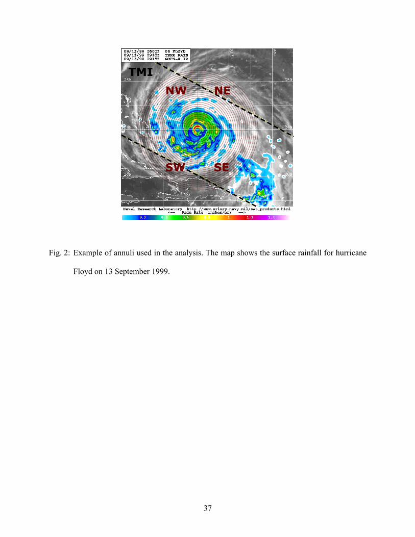
Fig. 2: Example of annuli used in the analysis. The map shows the surface rainfall for hurricane

Floyd on 13 September 1999.

37

Fig. 3: TRMM/TMI TC data coverage as a function of distance from the TC center, computed

relative to the maximum possible coverage. The maximum possible coverage for one 10-

km wide annulus around the TC center is defined as the number of TRMM overpasses

multiplied by the area within the annulus.

38

Fig. 4: TRMM/TMI surface rainfall (in mm h-1) of Hurricane Dennis, on 28 August 1999. The

dots indicate the location of the phase maximum of the rainfall asymmetry as a function

of the distance to the storm center. The circles (broken lines) are drawn at 50 km radial

increments.

39

Fig. 5: Radial profile of azimuthally averaged rain rates for Dennis on 28 August 1999.

40

Fig. 6: PDF of rainfall for Dennis within 300 km radius of the storm center.

41

Fig. 7: Radial variation of PDF for Dennis, from the storm center to 300 km radius. The black

line shows the azimuthal mean rain rate as a function of the radial distance to Dennis’

center.

42

Fig. 8: Same as Fig. 7, except for the rainfall flux, defined the rainfall multiplied the area that it

affects.

43

Fig. 9: Normalized phase maximum of the first-order rainfall asymmetry in Hurricane Dennis, as

a function of the distance from the storm center. The first order Fourier coefficients are

calculated relatively to the storm motion direction.

44

Fig. 10: Probability density functions calculated within 500 km radius of storm center a) for all

2121 observations, b) for TC intensity groups, and c) for oceanic basin sub groups.

45

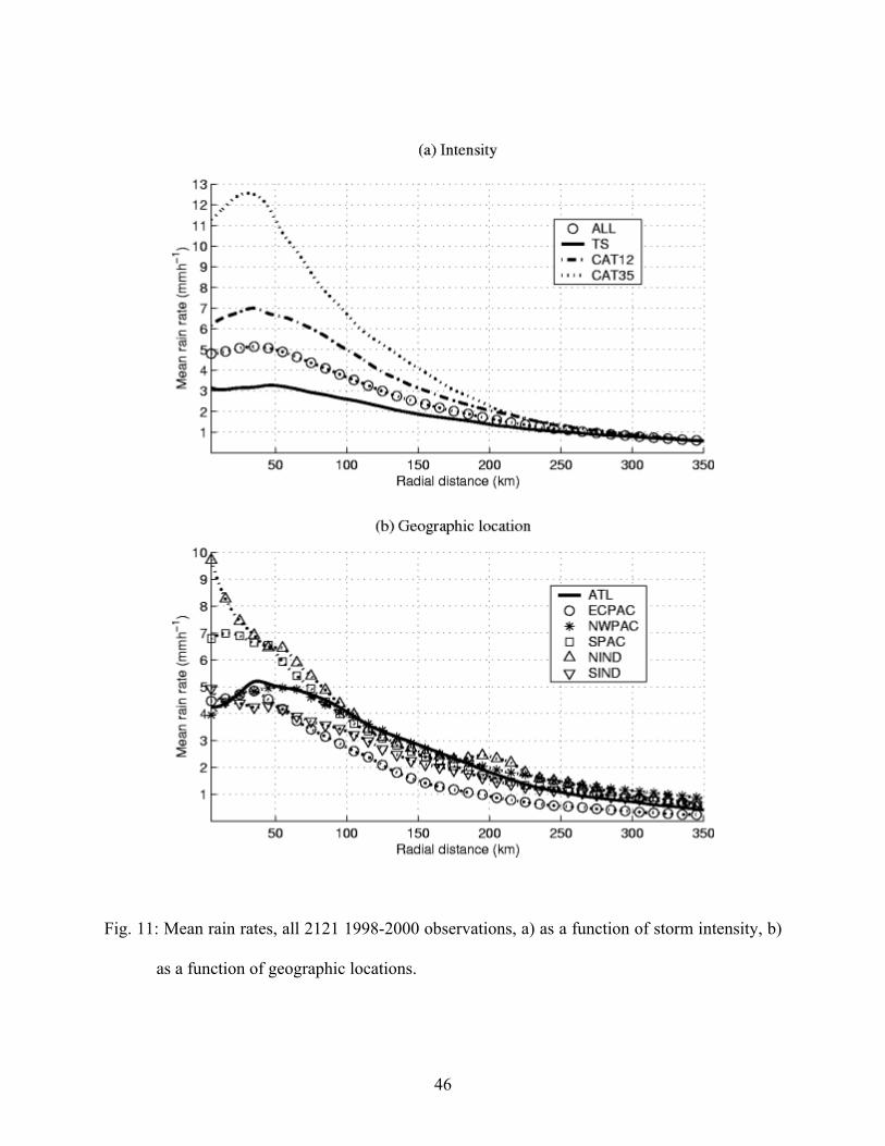
Fig. 11: Mean rain rates, all 2121 1998-2000 observations, a) as a function of storm intensity, b)

as a function of geographic locations.

46

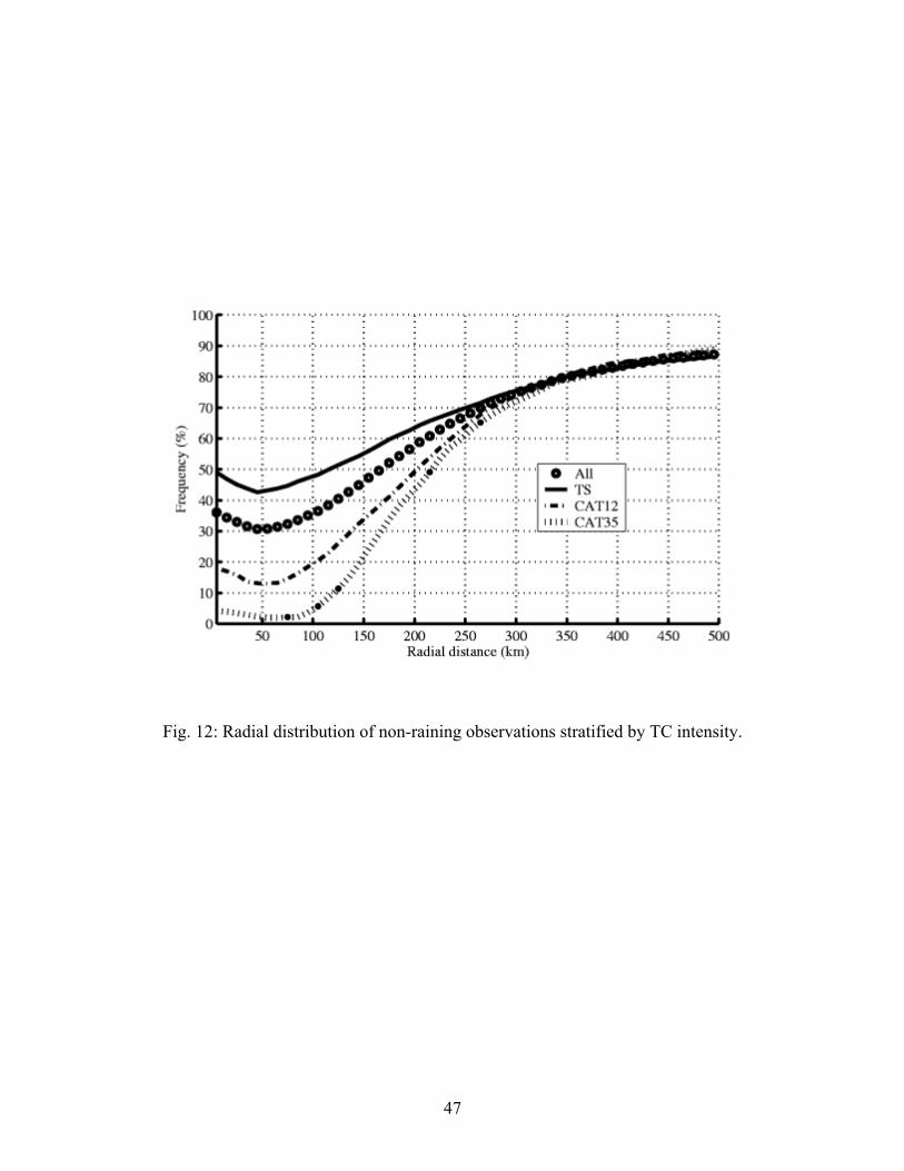
Fig. 12: Radial distribution of non-raining observations stratified by TC intensity.

47

Fig. 13: Radial distribution of rainfall PDF computed for 2121 observations. The color scale

refers to the frequency of occurrence of rain rates (in dBR scale) at any radial distance

from the center. The black line shows the azimuthal mean rainfall with radial distance.

48

Fig. 14: Radial distribution of rainfall PDFs for a) TS, b) CAT12, and c) CAT35 storms. The

color scale and black lines are as described in Fig. 13.

49

Fig. 15: Same as Fig. 13, except for the rainfall flux. The rainfall flux is defined as the rainfall

rate multiplied by the affected area. Therefore, one 10 mm h-1 observation weighs as

much as ten 1 mm h-1 observations in the PDF of rainfall flux; 1 and 10 mm h-1 weigh the

same in the PDF of rainfall (Fig. 13).

50

Fig. 16: Same as Fig. 14, except for the rainfall fluxes.

51

Fig. 17: Rainfall asymmetry calculated in 10 km rings around the storm center, as a function of

storm intensity: a) 2121 TC observations (total distribution), b) TS, c) CAT12, d)

CAT35. The storm motion vector is aligned with the positive y-axis. The color scale

indicates the amplitude of the normalized asymmetry. The red corresponds to the

maximum positive anomaly and the blue the minimum rainfall within the storm.

52

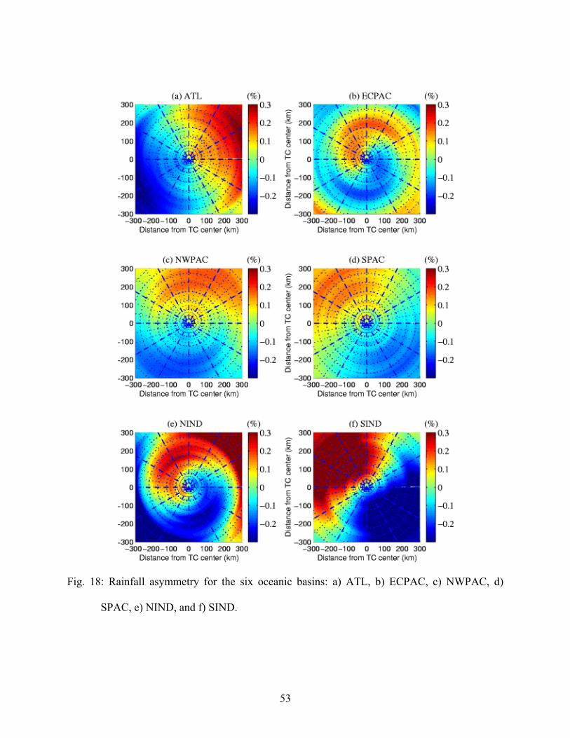
Fig. 18: Rainfall asymmetry for the six oceanic basins: a) ATL, b) ECPAC, c) NWPAC, d)

SPAC, e) NIND, and f) SIND.

53

Fig. 19: Rainfall Asymmetry as a function of the storm translation speed: a) v<5ms-1, and b)

v>5ms-1.

54