Precession, nutation, and space geodetic determination of the
13
HAL Id: hal-00120000 https://hal.sorbonne-universite.fr/hal-00120000v2 Submitted on 30 Jun 2011 HAL is a multi-disciplinary open access archive for the deposit and dissemination of sci- entific research documents, whether they are pub- lished or not. The documents may come from teaching and research institutions in France or abroad, or from public or private research centers. L’archive ouverte pluridisciplinaire HAL, est destinée au dépôt et à la diffusion de documents scientifiques de niveau recherche, publiés ou non, émanant des établissements d’enseignement et de recherche français ou étrangers, des laboratoires publics ou privés. Precession, nutation, and space geodetic determination of the Earth’s variable gravity field G. Bourda, Nicole Capitaine To cite this version: G. Bourda, Nicole Capitaine. Precession, nutation, and space geodetic determination of the Earth’s variable gravity field. Astronomy and Astrophysics - A A, EDP Sciences, 2004, 428, pp.691-702. <10.1051/0004-6361:20041533>. <hal-00120000v2>
Transcript of Precession, nutation, and space geodetic determination of the

HAL Id: hal-00120000https://hal.sorbonne-universite.fr/hal-00120000v2
Submitted on 30 Jun 2011
HAL is a multi-disciplinary open accessarchive for the deposit and dissemination of sci-entific research documents, whether they are pub-lished or not. The documents may come fromteaching and research institutions in France orabroad, or from public or private research centers.
L’archive ouverte pluridisciplinaire HAL, estdestinée au dépôt et à la diffusion de documentsscientifiques de niveau recherche, publiés ou non,émanant des établissements d’enseignement et derecherche français ou étrangers, des laboratoirespublics ou privés.
Precession, nutation, and space geodetic determinationof the Earth’s variable gravity field
G. Bourda, Nicole Capitaine
To cite this version:G. Bourda, Nicole Capitaine. Precession, nutation, and space geodetic determination of the Earth’svariable gravity field. Astronomy and Astrophysics - A
A, EDP Sciences, 2004, 428, pp.691-702. <10.1051/0004-6361:20041533>. <hal-00120000v2>
A&A 428, 691–702 (2004)DOI: 10.1051/0004-6361:20041533c© ESO 2004
Astronomy&
Astrophysics
Precession, nutation, and space geodetic determinationof the Earth’s variable gravity field
G. Bourda and N. Capitaine
Observatoire de Paris, SYRTE/UMR 8630-CNRS, 61 avenue de l’Observatoire, 75014 Paris, Francee-mail: [email protected]; e-mail: [email protected]
Received 25 June 2004 / Accepted 10 August 2004
Abstract. Precession and nutation of the Earth depend on the Earth’s dynamical flattening, H, which is closely related to thesecond degree zonal coefficient, J2 of the geopotential. A small secular decrease as well as seasonal variations of this coefficienthave been detected by precise measurements of artificial satellites (Nerem et al. 1993; Cazenave et al. 1995) which have to betaken into account for modelling precession and nutation at a microarcsecond accuracy in order to be in agreement with theaccuracy of current VLBI determinations of the Earth orientation parameters. However, the large uncertainties in the theoreticalmodels for these J2 variations (for example a recent change in the observed secular trend) is one of the most important causes ofwhy the accuracy of the precession-nutation models is limited (Williams 1994; Capitaine et al. 2003). We have investigated inthis paper how the use of the variations of J2 observed by space geodetic techniques can influence the theoretical expressions forprecession and nutation. We have used time series of J2 obtained by the “Groupe de Recherches en Géodésie spatiale” (GRGS)from the precise orbit determination of several artificial satellites from 1985 to 2002 to evaluate the effect of the correspondingconstant, secular and periodic parts of H and we have discussed the best way of taking the observed variations into account.We have concluded that, although a realistic estimation of the J2 rate must rely not only on space geodetic observations over alimited period but also on other kinds of observations, the monitoring of periodic variations in J2 could be used for predictingthe effects on the periodic part of the precession-nutation motion.
Key words. astrometry – reference systems – ephemerides – celestial mechanics – standards
1. Introduction
Expressions for the precession of the equator rely on values forthe precession rate in longitude that have been derived fromastronomical observations (i.e. observations that were basedupon optical astrometry until the IAU1976 precession, and thenon Very Long Baseline Interferometry (VLBI) observations formore recent models). The IAU2000 precession-nutation modelprovided by Mathews et al. (2002) (denoted MHB 2000 inthe following), that was adopted by the IAU beginning on1 January 2003, includes a new nutation series for a non-rigidEarth and corrections to the precession rates in longitude andobliquity that were estimated from VLBI observations during a20-year period. The precession in longitude for the equator be-ing a function of the Earth’s dynamical flattening H, observedvalues for this precession quantity are classically used to derivea realistic value for H. Such a global dynamical parameter ofthe Earth is generally considered as a constant, except in a fewrecent models for precession (Williams 1994; Capitaine et al.2003) or nutation (Souchay & Folgueira 1999; Mathews et al.2002; Lambert & Capitaine 2004) in which either the secular orthe zonal variations of this coefficient are explicitly consideredthrough simplified models.
The recent implementation of the IAU2000 A precession-nutation model guarantees an accuracy of about 200 µas inthe nutation angles, and all the predictable effects that haveamplitudes of the order of 10 µas have therefore to be con-sidered. One of these effects is the influence of the varia-tions (∆H) in the Earth’s dynamical flattening, which are notexplicitly considered in the IAU2000 A precession-nutationmodel. Furthermore, the IAU2000 precession is based on animprovement of the precession rates values derived from recentVLBI measurements, but it does not improve the higher degreeterms in the polynomials for the precession angles ψA, ωA ofthe equator (see Fig. 1). This precession model is not dynam-ically consistent because the higher degree precession termsare actually dependent on the precession rates (Capitaine et al.2003) and need to be improved, even though VLBI observa-tions are unable to discriminate between recent solutions dueto the limited span of the available data (Capitaine et al. 2004).One alternative way for such an improvement is to improve themodel for the geophysical contributions to the precession an-gles and especially the influence of ∆H (or equivalently ∆J2).
The H parameter is linked to the dynamical form-factor, J2 for the Earth (i.e. the C20 harmonic coefficient ofthe geopotential) which is determined by space geodetic tech-niques on a regular basis. Owing to the accuracy now reached
Article published by EDP Sciences and available at http://www.aanda.org or http://dx.doi.org/10.1051/0004-6361:20041533
692 G. Bourda and N. Capitaine: Precession, nutation, and Earth variable gravity field
γ
γ0
m
ψA
Ecliptic of date
χA
ε
ε 0
A
ω A
Mean equator of date
Mean equator of epoch
Ecliptic of epoch J2000
Fig. 1. Angles ψA and ωA for the precession of the equator: γm is themean equinox of the date and γ0 is the equinox of the epoch J2000.0.
by these techniques, the temporal variation of a few Earth grav-ity field coefficients, especially ∆C20, can be determined (forearly studies, see for example Nerem et al. 1993; Cazenaveet al. 1995; or Bianco et al. 1998). They are due to Earthoceanic and solid tides, as well as mass displacements of geo-physical reservoirs and post-glacial rebound for ∆C20. This co-efficient C20 can be related to the Earth’s orientation param-eters and more particularly to the Earth precession-nutation,through H. The purpose of this paper is to use space geode-tic determination of the geopotential to estimate ∆H, in orderto investigate its influence on the precession-nutation model.The C20 data used in this study have been obtained from thepositioning of several satellites between 1985 and 2002. We es-timate also the constant part of H, based on such space geodeticmeasurements, and compare its value and influence on preces-sion results with respect to those based on VLBI determina-tions.
In Sect. 2 we recall the equations expressing the equatorialprecession angles as a function of the dynamical flattening H.We provide the numerical values implemented in our model,compare the values obtained for H by various studies and dis-cuss the methods on which they rely. In Sect. 3 the relationshipbetween ∆H and ∆C20 is discussed, depending on the methodimplemented. We explain how these geodetic data are takeninto account in Sect. 4. We present our results in Sect. 5, anddiscuss them in the last part. We investigate how the use of ageodetic determination of the variable geopotential can influ-ence the precession-nutation results, considering first the pre-cession alone, and second the periodic contribution.
In the whole study, the time scale for t is TT Julian centuriessince J2000, which will be denoted cy.
2. Theoretical effect of ∆H on precession
This section investigates the theoretical effect of the varia-tions ∆H in the Earth’s dynamical flattening on the precessionexpressions.
2.1. Relationship between H and the precessionof the equator
The two basic angles ψA and ωA (see Fig. 1) for the preces-sion of the equator are provided by the following differential
equations (see Eq. (29) of Williams (1994) or Eq. (24) ofCapitaine et al. (2003)):
sinωAdψA
dt=
(rψ sin εA
)cosχA − rε sinχA
dωA
dt= rε cosχA +
(rψ sin εA
)sinχA (1)
where rψ and rε are respectively the precession rates in lon-gitude and obliquity, εA is the obliquity of the ecliptic ofdate and χA the planetary precession angle, determining theprecession of the ecliptic. Updated expressions for these pre-cession quantities are given in Capitaine et al. (2003). An ex-pression for the precession rates, rψ in longitude and rε in obliq-uity, is provided in detail in Williams (1994) and Capitaineet al. (2003) as a function of various contributions. The preces-sion rate in longitude can be written as rψ = r0+r1 t+r2 t2+r3 t3
where the largest first-order term in r0 is the luni-solar con-tribution denoted f01 |LS
cos ε0, where ε0 is the obliquity of theecliptic at J2000. It is such that (Kinoshita 1977; Dehant &Capitaine 1997):
f01 |LS= km M0 + ks S 0 (2)
in which M0 and S 0 are the amplitudes of the zero-frequencyMoon and Sun attractions, respectively, and:
km = 3 Hmm
mm + m⊕1
F23
n2m
Ω= H Km (3)
ks = 3 Hm
m + mm + m⊕n2Ω= H Ks. (4)
In the above expressions, H is the Earth’s dynamical flatten-ing, mm, m and m⊕ are the masses of the Moon, the Earth andthe Sun, respectively, nm is the Moon mean motion around theEarth, n the Earth mean motion around the Sun,Ω is the meanangular velocity of the Earth and F2 a factor for the mean dis-tance of the Moon. Current numerical values for such a prob-lem are (Souchay & Kinoshita 1996):
M0 = 496 303.66× 10⁻⁶
S 0 = 500 210.62× 10⁻⁶
km = 7546.′′7173289 /cy (5)
ks = 3475.′′1883295 /cy
f01 |LScos ε0 = 5040.′′6445 /cy
and (see Kinoshita 1977):
F2 = 0.999093142.
Hence, the link between the precession of the equator(ψA and ωA angles) and the Earth’s dynamical flattening (H)is shown by Eqs. (1)−(4) and (7) of Sect. 2.2. Classically, H isrelated to f01 |LS
derived from observations by:
H =f01 |LS
Km M0 + Ks S 0· (6)

G. Bourda and N. Capitaine: Precession, nutation, and Earth variable gravity field 693
Table 1. Comparison between constants used for different determinations of the dynamical flattening (H): (1) the precession rate in longi-tude (ψ1); (2) the speed of the general precession in longitude (p1); (3) the geodesic precession (pg); and (4) the obliquity of the eclipticat J2000.0 (ε0). The observational value actually used for each study is written in bold.
(1) (2) (3) (4)Sources H ψ1 p1 pg ε0
(× 103) (———————– in ′′/cy ———————)
Lieske et al. (1977) 5038.7784 5029.0966 −1.92 2326′21.′′448
Kinoshita (1977) and Seidelmann (1982) 3.2739935 5038.7784 5029.0966 −1.92 2326′21.′′448
Williams (1994) 3.2737634 5038.456501 5028.7700 −1.9194 2326′21.′′409
Souchay & Kinoshita (1996) 3.2737548 – 5028.7700 −1.9194 2326′21.′′448
Bretagnon et al. (1997) 3.2737671 5038.456488 5028.7700 −1.919883 2326′21.′′412
Bretagnon et al. (2003) – 5038.478750 5028.792262 −1.919883 2326′21.′′40880
Fukushima (2003) 3.2737804 5038.478143 5028.7955 −1.9196 2326′21.′′40955
Capitaine et al. (2003) 3.27379448 5038.481507 5028.796195 −1.919883 2326′21.′′406
Mathews et al. (2002) 3.27379492 5038.478750 5028.7923 −1.9198 2326′21.′′410
2.2. Astronomical determination of H
We can write r0 as:
r0 = f01 |LScos ε0 + f01 |PL
cos ε0 (7)
+H × lunisolar second order effects
+H × (J2 and planetary
)tilt effects
+J4 lunisolar effect
−geodesic precession
+non-linear effects (Mathews et al. 2002)
where f01 |PLis the first order term of the planetary contribu-
tion (also proportional to H). Classically, H is derived from ob-servationally determined values of r0. The measurement of r0
should be corrected by removing the modelled contributionsother than the lunisolar first order effect (see Eq. (7)). Hence,we obtain a value for f01 |LS
, which is the only term with suffi-ciently large amplitude (of the order of 5000′′/cy) to be sensi-tive to small changes in the value of the dynamical ellipticity Hof the Earth (see Eq. (6)). So, given the other contributions pro-vided by the theory, we can derive the value of H from the ob-served value of r0 and the model for the lunisolar first ordereffects.
A major problem consists in choosing the constant valueof H. Indeed, depending on the authors, it differs by about 10−7
(Table 1). This is due to the different measurements and modelsimplemented (see Fig. 1 of Dehant & Capitaine 1997; Fig. 5 ofDehant et al. 1999). On the one hand the optical measurementsgive values of the general precession in longitude pA referred tothe ecliptic of date, whereas VLBI gives measurements relativeto space. On the other hand, the various constants and modelsused for obtaining the value for H from a measured value (op-tical, Lunar laser ranging or VLBI) are different depending onthe study considered (see Eq. (7)).
Classically, ψA is developed in a polynomial form of tas: ψA = ψ0 + ψ1 t + ψ2 t2 + ψ3 t3. In Table 1, we recall thedifferent values used (i) for ψ1 (i.e. the precession rate in lon-gitude, ψ1 = r0), directly obtained from VLBI measurements,
and (ii) for p1 which is the observationally determined value ofprecession in the optical case: ψ1 = p1+χ1 cos ε0 (Lieske et al.1977).
The computation of the IAU2000 precession-nutationmodel by Mathews et al. (2002) is based on a new methodwhich uses geophysical considerations. They adjust nine BasicEarth Parameters (BEP), including the Earth dynamical flatten-ing H.
2.3. Method and parameters used in this study
Based on the paper by Capitaine et al. (2003), denoted here-after P03, we use differential Eq. (1) in which H has been re-placed by H + ∆H (using Eqs. (2)−(4) and (7)). We start fromthe P03 initial values for the variables ωA, ψA, εA, χA and pA,that are represented as polynomials of time and rely on thenumerical values given in Table 2. We solve Eq. (1) togetherwith the other precession equations (e.g. see Eqs. (26) and (28)of P03) with the software GREGOIRE (Chapront 2003) thatcan process Fourier and Poisson expressions. We iterate thisprocess until we obtain a convergence of the solution.
3. Relationship between C20 and H
3.1. Relation
From the geodetic C20 variation series we can derive the cor-responding variations of the dynamical flattening H. Indeed,knowing that J2 = − C20 = −
√5 C20, in the case of a rigid
Earth, we can write (see Lambeck 1988):
H =(C − A + B
2
)/C =
M Re2
CJ2 (8)
= −M Re2
CC20
= −√5M Re
2
CC20

694 G. Bourda and N. Capitaine: Precession, nutation, and Earth variable gravity field
Table 2. Numerical values used in this study. H, ψ1 and ω1 are inte-gration constants.
Initial values at J2000.0
H HMHB = 3.27379492 × 10⁻³
ψ1 5038.′′481507/cy
ω1 −0.′′02575/cy
p1 5028.′′796195/cy
χ1 10.′′556403/cy
ε0 84 381.′′406 = 2326′21.′′406
Contributions to the precession rate in longitude (in ′′/cy)
Lunisolar first order 5494.062986 × cos ε0 5040.7047
Planetary first order 0.031
Geodesic precession −1.919882
where A, B and C are the mean equatorial and polar momentsof inertia of the Earth. M and Re are respectively the mass andthe mean equatorial radius of the Earth. C20 is the normalizedStokes coefficient (of degree 2 and order 0) of the geopotential.
But the Earth is elastic, so let us consider small variationsof H, C20 and the third principal moment of inertia of the Earth(C being its constant part and c33 its variable part). Then weobtain:
H total =M Re
2
C1
1 + c33C
J2 total (9)
c33/C being a small quantity of the order of 10−6, we considerthe Taylor development of (1 + c33/C)−1. Then the total expres-sion of H can be written as:
H total =MRe
2
CJ2 total
(1 − c33
C+
(c33
C
)2+ ...
)(10)
where MRe2/C × (c33/C)n J2 for n ≥ 1 is smaller than 10−11.
So, in Eq. (10), considering (i) constant and variable parts sep-arately; and (ii) Eq. (8), we obtain:
∆H =MRe
2
C∆J2 = −
√5
MRe2
C∆C20 (11)
where∆J2 = −∆C20 = −√
5∆C20 corresponds to the variationsof the Stokes coefficient J2. Generally, we can write: ∆J2 ∝c33/C (Lambeck 1988).
3.2. Computation of the ratio MRe2/C
The coefficient MRe2/C is usually obtained from the H and J2
values (see Eq. (8)). In order to determine the constant partof H, we can use (i) the Re, M and C values; or (ii) the Clairauttheory (see Table 3).
First, recall the Earth geometrical flattening ε:
ε =Re − Rp
Re(12)
where Rp and Re are respectively the polar and equatorial meanradii of the Earth. Second, recall the assumptions that theEarth (i) is in hydrostatic equilibrium; and (ii) is considered asa revolutional ellipsoid. Hence, the first Clairaut equation givesthe Earth geometrical flattening as a function of J2 and q. Theapproximations to the first and second order are respectively:
ε =q2+
32
J2 (13)
ε =q2+
32
J2 +98
J22 − 3
14J2 q − 11
56q2 (14)
where the geodynamical constant is:
q =ω2Re
3
GM(15)
= 3.461391× 10⁻³, IAG (Groten 1999).
Then, the following Radau equation can help us to determinethe expression of MRe
2/C:
ε − q/2H
= 1 − 25
√1 + η =
1λ
(16)
where λ is the d’Alembert parameter and η the Radau parame-ter, as:
η =5q2ε− 2. (17)
Hence, replacing ε with Eq. (13) in Eq. (16) and using Eq. (8)gives the Darwin-Radau relation as following:
C
MRe2=
23λ=
23
(1 − 2
5
√1 + η
). (18)
Our tests have shown that Eq. (14) for ε, in the expression (17)of η, gives more reliable results.
In Table 3 we compare the various H values obtained. Wedenote (i) H∗ the value obtained with the Clairaut methodand (ii) H∗∗ the value obtained using directly the Re, Cand M values. Both are computed with Eq. (8) and a valuefor J2 of 1.0826358 × 10⁻³. Note that in contrast, IAGor MHB values (usually used) are determined from astro-nomical precession observations and can be used to com-pute the C/MRe
2 value. We can add that the differenceswith HMHB come from (i) the hydrostatic equilibrium hypoth-esis in Clairaut’s theory for the value H∗; and (ii) the poorlydetermined Re, C and M values, for the value H∗∗. This willintroduce errors in the ∆H determination, which we will studyin Sect. 3.3.
In the following, we will use the C/(MRe
2)
valuedetermined with the Clairaut theory, noted with a (*)in Table 3, which corresponds to a value for Hof: H∗ = 3.26715240× 10⁻³.
3.3. Error estimation
We can estimate the error that the use of the Clairaut the-ory introduces into the ∆H results. Indeed, if we consider theMHB value as the realistic H value (see Table 3), the relativeerror made is:
σH =HMHB − H∗
HMHB 2 × 10⁻³. (19)

G. Bourda and N. Capitaine: Precession, nutation, and Earth variable gravity field 695
Table 3. Comparison between different values of the coefficient C/(MRe
2)
and of the constant part for H: (1) IAG values (Groten 1999)– (2) MHB values (Mathews et al. 2002) – (3) Constant part H∗∗ obtained from Eq. (8) using the M, Re and C IAG values – (4) Method of“Clairaut” (Sect. 3.2), assuming hydrostatic equilibrium. The third and fourth methods use a constant part for C20 of −4.841695×10⁻⁴ in Eq. (8)(i.e. J2 = 1.0826358 × 10⁻³). The sense of the computation is indicated by the arrows.
(1) (2) (3) (4)IAG (1999) MHB 2000 Separate values for Clairaut
M, Re and C Theory
C/(M Re
2)
0.330701 0.330698 0.330722∗∗ 0.331370∗
±2 × 10⁻⁶
⇑ ⇑ ⇓ ⇓H 3.273763 × 10⁻³ 3.27379492 × 10⁻³ H∗∗ = 3.27355562 × 10⁻³ H∗ = 3.26715240 × 10⁻³
±2 × 10⁻⁸
We estimate that the error is about 0.2%. So, computing thevariable part of H with the C20 data results in a maximum errorof about:
|∆Hreal − ∆H∗| (2 × 10⁻³
)×
(6 × 10⁻⁹
)
1.2 × 10⁻¹¹ (20)
assuming that the maximum value for ∆H is of the order of 6×10⁻⁹. Then, regarding the values of the ∆H data and of theirprecision, we can consider this error as negligible.
4. Time series of ∆C20 used in this study
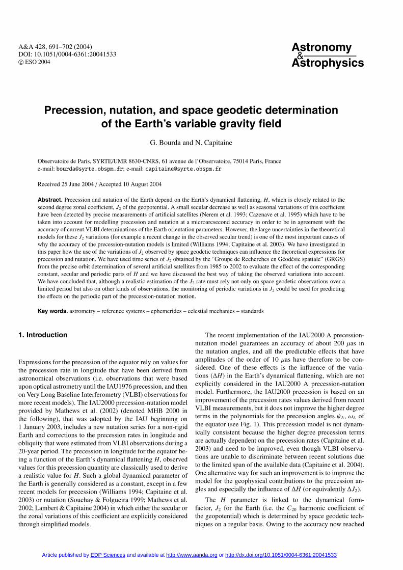
The geodetic data used are the time series (variable part) ofthe spherical harmonic coefficient C20 of the geopotential,obtained by the GRGS (Groupe de Recherche en GéodésieSpatiale, Toulouse) from the precise orbit determination of sev-eral satellites (like LAGEOS, Starlette or CHAMP) from 1985to 2002 (Biancale et al. 2002). The combination of these satel-lites allows the separation of the different zonal geopotentialcoefficients, more particularly of J2 and J4. This series in-cludes (i) a model part for the atmospheric mass redistribu-tions (Chao & Au 1991; Gegout & Cazenave 1993) and forthe oceanic and solid Earth tides (McCarthy 1996); and (ii) aresidual part (see Fig. 2) obtained as difference of the spacemeasurements with respect to a model. These various changesin the Earth system are modelled as variations in the standardgeopotential coefficient C20 and we note the different contribu-tions ∆C20atm , ∆C20oc , ∆C20soltid and ∆C20res , respectively.
4.1. ∆C20 residuals and its secular trend: Observedpart
Earlier studies already took into account the effect of the sec-ular variation of C20 on the precession of the equator. Sucha secular variation is attributed to the post-glacial reboundof the Earth (Yoder et al. 1983), which reduces its flatten-ing. Williams (1994) and Capitaine et al. (2003) considereda J2 rate value of −3 × 10⁻⁹/cy. Using the numerical value ofTable 2 for the first order contribution ( f01 cos ε0) to the pre-cession rate r0, which is directly proportional to J2, the con-tribution J2/J2 × f01 cos ε0 of the J2 rate to the accelerationof precession d2ψA/dt2 is about −0.014′′/cy2, giving rise to
1985 1990 1995 2000-4e-10
-3e-10
-2e-10
-1e-10
0
1e-10
2e-10
3e-10 C20 residuals without constant part
1985 1990 1995 2000Years
-2e-10
-1e-10
0
1e-10
2e-10Filtered C20 residuals without constant part
Fig. 2. Normalized ∆C20 residuals (top: raw residuals, bottom: filteredresiduals, where the high frequency signals have been removed): non-modelled part of the ∆C20 harmonic coefficient of the Earth gravityfield.
a −0.007′′/cy2 contribution to the t2 term in the expressionof ψA.
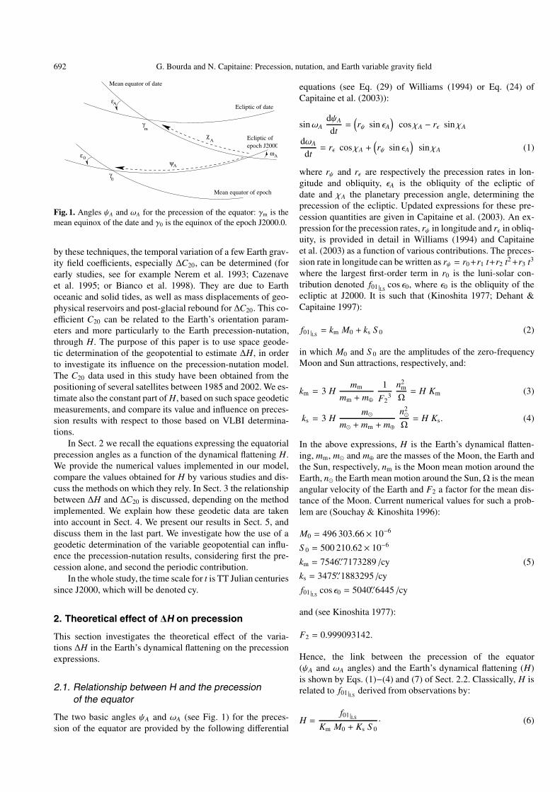
Since 1998, a change in the secular trend of the J2 data hasbeen reported (Cox & Chao 2000). This change can be seen inthe series of ∆C20 residuals (see Fig. 2). An attempt to modelthis effect, with oceanic data, water coverage data and geo-physical models, has been investigated by Dickey et al. (2002).Using the residuals ∆C20 of the GRGS, we can estimate a secu-lar trend for J2 = −
√5 C20 from 1985 to 1998 (see Fig. 3). We
find a J2 rate of the order of: −2.5 (±0.2)×10−9/cy, which gives

696 G. Bourda and N. Capitaine: Precession, nutation, and Earth variable gravity field
1985 1990 1995 2000
-5e-10
0
5e-10
J2 residualsLinear regression
1985 1990 1995 2000Years
-4e-10
-2e-10
0
2e-10
4e-10
6e-10
J2 filtered residualsLinear regression
Fig. 3. J2 GRGS residuals (top: raw residuals, bottom: filtered residu-als, where the high frequency signals have been removed): estimationof the linear trend, from 1985 to 1998.
a change of about −0.006′′/cy2 in the t2 term of the polynomialdevelopment of the precession angle ψA.
As this secular trend is not the same in the total data span,we will also model the long term variations in the C20 resid-ual series with a periodic signal. Such a long-period term inthe J2 residual series may come from mismodelled effects, par-ticularly from the 18.6-yr solid Earth tides. We will make suchan assumption and adjust for the period 1985−2002, a secu-lar trend and a long-period term in the ∆C20 residual series(see Sect. 4.3).
However, it should be noted that a secular trend for J2,of the order of −3 × 10⁻⁹/cy, is more consistent with longterm studies of the Earth rotation variations by Morrison &Stephenson (1997), based upon eclipse data over two millen-nia (they found J2 = (−3.4 ± 0.6) × 10−9/cy).
4.2. ∆C20 geophysical data used: Modelled part
The geophysical models that have been previously subtractedfrom the C20 data (i.e. atmospheric, oceanic and solid Earthtides effects) must be added back to these data in exactly thesame way they had been subtracted to reconstruct the relevantgeophysical contributions.
For each contribution we give the associated potential U atthe point (r, φ, λ, t) (limited to the degree 2 and order 0) thatwe identify with the Earth gravitational potential. Hence, we
1985 1990 1995 2000
-2e-10
-1e-10
0
1e-10
2e-10
3e-10
1985 1990 1995 2000Years
-1e-10
-5e-11
0
5e-11
1e-10
1,5e-10
Filtered and interpolated atmospheric C20
Fig. 4. Normalized atmospheric ∆C20 (top: raw data, bottom: filtereddata, where the high frequency signals have been removed): atmo-spheric modelled part of the ∆C20 harmonic coefficient of the Earthgravity field, obtained with ECMWF pressure data.
obtain the ∆C20 coefficient contribution of each geophysicalsource.
• The atmospheric contribution is due to pressure changesin time, measured and given by the European Centre forMedium-range Weather Forecasts (ECMWF) (see Fig. 4).The simple-layer atmospheric potential, limited to degree 2and order 0, can be expressed as:
Uatm = 4πGRe1 + k
′2
5g
(Re
r
)3
∆C20ECMWF(t) P20(sinφ) (21)
where G = 6.672×10⁻¹¹ m3 kg−1 s−2 is the gravitational con-stant, k
′2 = −0.314166 is a Love number (Farrell 1972), g =
9.81 m s−2, and P20(sinφ) is the Legendre function of de-gree 2 and order 0. The C20ECMWF(t) atmospheric coefficient,expressed in Pascals, comes from the spherical harmonic de-composition of the ECMWF atmospheric pressure grids, ev-ery 6 h, over continents (see Gegout & Cazenave 1993; orChao & Au 1991):
∆C20ECMWF(t) =∫
S∆p (φ, λ, t)
(32
sin2 φ − 12
)dS (22)
where S is a surface grid pressure around the Earth and ∆pis the difference of pressure with a constant part prefixed, atthe point (φ, λ). Hence, identifying Eq. (21) with the Earth

G. Bourda and N. Capitaine: Precession, nutation, and Earth variable gravity field 697
1985 1990 1995 2000
-4e-10
-2e-10
0
2e-10
4e-10
1985 1990 1995 2000Years
0
5e-11
1e-10
1,5e-10
Filtered and interpolated ocean tides C20
Fig. 5. Normalized oceanic ∆C20 (top: raw data, bottom: filtered data,where the high frequency signals have been removed): oceanic-tide-modelled part of the ∆C20 harmonic coefficient of the Earth gravityfield; IERS Conventions 1996.
gravitational potential, we obtain the atmospheric pressurecontribution to the ∆C20 harmonic coefficient:
∆C20atm(t) =4π Re
2 (1 + k′2)
5Mg∆C20ECMWF(t)· (23)
• The contribution of the oceanic tides (see Fig. 5) is modelledin the IERS Conventions 1996. The Earth responds to the dy-namical effects of ocean tides, and the associated potential,limited to the degree 2 and order 0, is:
Uoc = 4π G Re ρw1 + k
′2
5
(Re
r
)3
P20(sin φ) α(t) (24)
where we note α, depending on time, as:
α =∑
n
−∑
+
C±n,2,0 cos(θn(t)+ χn)+ S ±n,2,0 sin(θn(t)+ χn).(25)
The sum over n corresponds to the Doodson developmentwhose associated arguments are θn and χn. The parame-ter ρw (=1025 kg m−3) is the mean density of sea wa-ter. Furthermore, C±n,2,0 = C±n,2,0 sin(ε±n,2,0) and S ±n,2,0 =C±n,2,0 cos(ε±n,2,0), where C±n,2,0 and ε±n,2,0 are the normalizedamplitude and phase of the harmonic model of the oceanictides limited to degree 2 and order 0. Identifying Eq. (24)with the Earth gravitational potential gives the oceanic tidecontribution to the ∆C20 harmonic coefficient:
∆C20oc(t) =4π Re
2 (1 + k′2) ρW
5 Mα(t). (26)
1985 1990 1995 2000
-6e-09
-5e-09
-4e-09
-3e-09
-2e-09
1985 1990 1995 2000Years
-5e-09
-4,5e-09
-4e-09
-3,5e-09
-3e-09
Filtered and interpolated solid earth tides C20
Fig. 6. Normalized solid tides ∆C20 (top: raw data, bottom: filtereddata, where the high frequency signals have been removed): solid-Earth-tide-modelled part of the ∆C20 harmonic coefficient of the Earthgravity field; IERS Conventions 1996.
• The solid Earth tide contribution (see Fig. 6) is due to thegravitational effect of the Moon and the Sun on the Earth(IERS Conventions 1996). This force derives from a poten-tial, developed in spherical harmonics, which limited to de-gree 2 and order 0 is:
Usoltid = G MRe
2
r3P20(sin φ) C20Moon+Sun (t) (27)
where
C20Moon+Sun(t) =k20 Re
3
5 M
sun∑
p=moon
mp
r3p
P20(sinφp)
(28)
where k20 = 0.3019 is the nominal degree Love number fordegree 2 and order 0, mp the mass of the body p, and rp
the geocentric distance and φp the geocentric latitude at eachmoment of the body p. The Love number depends on thetidal frequencies acting on the Earth. Hence, the contribu-tion to ∆C20 from the long period tidal constituents of vari-ous frequencies ν must be corrected (see IERS Conventions1996). Equation (27) corrected for the frequency dependenceof the Love number, can be identified with the Earth gravita-tional potential. We obtain the Earth solid tide contributionto the ∆C20 harmonic coefficient:
∆C20soltid (t) = C20Moon+Sun + “frequency correction”. (29)

698 G. Bourda and N. Capitaine: Precession, nutation, and Earth variable gravity field
1985 1990 1995 2000
-5e-10
0
5e-10
1e-09
1985 1990 1995 2000Years
-3e-10
-2e-10
-1e-10
0
1e-10
2e-10
3e-10
Fig. 7. Normalized total ∆C20: top is the total series including atmo-spheric, oceanic tides and solid earth tides effects and the residuals;bottom is the total series without the solid earth tides effect.
This contribution comprises a constant part in the ∆C20 solidEarth tide, which is called “permanent tide”. We haveestimated it and obtained: −4.215114 × 10⁻⁹ (the IERSConventions value is −4.201×10⁻⁹). We must remove it fromour ∆C20 data coming from solid Earth tides.• Finally, we must consider a series including all the effects
described before. Hence, we add them back to the residuals(Fig. 2), interpolating and filtering the data. Then we obtainthe total series (Fig. 7).
4.3. Adjustments in ∆H data
Equation (11) allows us to transform the geodetic ∆C20 tempo-ral variations into the dynamical flattening variations∆H. Theycan then be introduced into the precession Eq. (1), replacing Hwith (H + ∆H) (Eqs. (2)–(4) and (7)) and using the processalready described in Sect. 2.3.
It is generally considered that VLBI observations of theEarth’s orientation in space are not sensitive to the atmosphericand oceanic contributions to the variations in C20 (de Viron2004). However the amplitudes of these effects have been eval-uated in Table 11 for further discussion and in any case we cannotice that they have a negligible effect on precession.
The analytical and semi-analytical approach to solving theprecession-nutation equations provides polynomial develop-ments of the ψA and ωA quantities. The ∆H data are then con-sidered as a linear expression plus Fourier terms with periods
Table 4. Summary of the constant parts for H and C20 (Constant part +Permanent tide) used in this study.
HMHB 3.2737942 × 10⁻³
C20 −4.841695 × 10⁻⁴
J2 1.0826358 × 10−3
H∗ 3.2671524 × 10−3
H∗ with geophysical 3.2671521 × 10⁻³
constant parts
H∗∗ 3.2735556 × 10⁻³
derived from a spectral analysis (18.6-yr, 9.3-yr, annual andsemi-annual terms) (see Tables 4–7). Note that the phaseangles used for adjusting the ∆H periodic terms are those of thecorresponding nutation terms. This implies changes in the de-velopment of the equatorial precession angles (ψA, ωA), whichwe describe in the next section.
For the residual contribution of ∆H, we will consider (i) anadjustment of a secular trend over the interval from 1985to 1998 (see Table 6 and Eq. (30)), and (ii) an adjustmentof a secular trend plus a 18.6-yr periodic term (see Table 5and Eq. (31)), both added to the seasonal terms. The fit (i) ofthe secular trend gives:
H −7.4 × 10⁻⁹/cy ⇔ J2 −2.5 × 10⁻⁹/cy (30)
and the fit of model (ii) gives:
∆H =(74 × 10−11
)× t +
(20.9 × 10⁻¹¹
)× sin(ωt)
+(32.5 × 10⁻¹¹
)× cos(ωt) (31)
with ω = 2π/0.186.We must recall that these adjustments have been made to-
gether with the fit of annual and semi-annual terms. In contrast,the higher frequency terms appearing in the ∆H data have beenfiltered and we therefore did not take into account other con-tributions, as for example the diurnal effects of the geophysicalcontributions in ∆H.
5. Effects of the ∆H contributionson the precession angles
On the basis of the models fitted to the time series of ∆H inthe previous section, obtained with geodetic ∆C20 series, weinvestigate the influence of these geodetic data on the preces-sion angle developments. First, we evaluate the effect of thesecular trend considered in the ∆C20 residual series. Second,we report on the influence of each geophysical contribution, onthe influence of the residuals and on that of the total contribu-tion. Finally we focus on the periodic effects resulting from thevarious ∆H contributions.
5.1.J2 influence
We have already mentioned that the J2 influence was takeninto account in previous precession solutions (Williams 1994;Capitaine et al. 2003) (see Sect. 4.1). But depending on the
G. Bourda and N. Capitaine: Precession, nutation, and Earth variable gravity field 699
Table 5. Adjustment of periodic terms in the ∆H contributions, for the data span 1985−2002 for various ∆H geophysical sources (atmo-spheric ∆H atm., oceanic tides ∆H oc. and solid earth tides ∆H soltid., as well as the residuals ∆H res.) – Units are in 10−10 rad.
Period ∆H res. ∆H atm. ∆H oc. ∆H soltid.(in years) sin cos sin cos sin cos sin cos
1 2.17 −4.02 0.96 −1.66 −3.92 1.41 −4.64 0.89
0.5 −0.43 3.71 0.76 1.56 −0.34 28.04
18.6 2.09 3.25 −0.46 −26.29
9.3 −0.17 −1.65 −0.01 0.29
Table 6. Specific adjustment of the ∆H residual series (∆H res.),from 1985 to 1998. The secular trend is considered as in Eq. (30) –Units are in 10−10 rad.
Period ∆H res.(in years) sin cos
1 2.57 −3.84
0.5 −0.50 3.80
Table 7. Adjustment of the total series of ∆H (∆H tot.), from 1985to 2002 – Units are in 10−10 rad.
Period ∆H tot.(in years) sin cos
1 −5.39 −3.39
0.5 0.07 33.67
18.6 0.92 −23.11
9.3 −0.08 −0.50
value adopted, the polynomial development of the ψA preces-sion angle is different. Indeed, if we take J2 = −2.5 × 10⁻¹¹/cylike in our study, or J2 = −3 × 10⁻¹¹/cy like in Capitaine et al.(2003), the contribution in ψA varies by about 1.5 mas/cy2 (seeTable 8). So we must carefully take into account this J2 rate.Furthermore, (i) we already noticed that such a secular trendhas been recently discussed because of the change in this trendin 1998 (see Fig. 2); and (ii) the uncertainty in this seculartrend, derived from space measurements of J2, is significant.Therefore we can conclude that until there is a better determi-nation of the J2 rate, the accuracy of the precession expressionis limited to about 1.5 mas/cy2.
5.2. Precession
First, we can compare the polynomial part of our solutionGeod04 for the precession angles, based on the constantpart HMHB of H and on its variable part provided by ex-pression (31), with previous precession expressions (IAU2000and P03) (see Table 9). The differences larger than one µasconcern the ψA precession angle and more particularly its t2
and t3 terms. The differences (of 7 mas and 2 µas, respec-tively) with respect to P03 are due to considering or not con-sidering the J2 effect. Actually, P03 includes a J2 secular
trend, whereas Geod04 includes instead a 18.6-yr periodic term(see (3) in Table 9 or (2) in Table 10). Comparing Geod04 withthe IAU2000 precession (which does not consider the J2 rate)shows differences of 0.6 mas and 5 µas in the t2 and t3 terms,respectively. This results from the improved dynamical con-sistency of the Geod04 solution (based on the P03 precessionequations) with respect to IAU2000. Note that such results re-garding the t2 and t3 terms will not be affected if changes ofthe order of 1 mas/cy in the precession rate would occur in anupdated P03 solution.
Second, we can evaluate the differences introduced inthe ψA (and ωA) polynomial development by the use of a con-stant part for H determined with the geodetic J2 (as used inGeod04-H* and Geod04-H**) instead of the Hastro determinedby VLBI and used in Geod04. Table 9 shows that the differ-ences are very large, but it should be noted that using J2 forderiving H suffers from the too large errors introduced by themismodelled C/MRe
2.
5.3. Periodic contributions
On the basis of the adjustments made in Sect. 4.3 for the dif-ferent ∆H contributions, we estimate here the periodic effectsappearing in the expressions of the precession angles. We canfocus on the Fourier terms in the ψA precession angle, whichare the most sensitive to the ∆H effects. The corresponding re-sults are presented in Table 11.
• First, we note that the major effect is due to the 18.6-yr peri-odic term in the solid Earth tides (contribution number (3) ofTable 11): about −2 µas and 120 µas in cosine and sine, re-spectively. The tidal annual and semi-annual effects are neg-ligible as well as the atmospheric and oceanic effects (con-tributions number (4) and (5) of Table 11).• Second, note that the ∆H variation strictly limited to its
residual part, not modelled into the geodetic orbit restitu-tion, introduces negligible Fourier terms into the ψA devel-opment. But we can note that the way the long term effectis considered in such data (i.e. either with a secular trendterm (contribution number (1) of Table 11) or a 18.6-yr pe-riodic term (contribution number (2) of Table 11)) is impor-tant. Modelling the long term variation in the geodetic resid-uals over the total data span as a 18.6-yr variation induces aterm with an amplitude of 15 µas in the ψA development. Butat present the ∆C20 data span is not long enough to allow usto discriminate between the two models.

700 G. Bourda and N. Capitaine: Precession, nutation, and Earth variable gravity field
Table 8. Influence of J2 on the polynomial development of ψA (more particularly on the t2 and t3 terms): (1) IAU2000 (Mathews et al. 2002);(2) P03 (Capitaine et al. 2003); and (3) Same computation as in P03 but with other J2 values. The J2 secular trend estimation based on our C20
residuals series is: J2 = −2.5 × 10⁻⁹/cy.
J2 t2 t3
(1) IAU2000 None −1.′′07259 −0.′′001147
(2) P03 −3 × 10⁻⁹/cy −1.′′079007 −0.′′001140
Differences wrt P03︷︸︸︷0 /cy −7.000 mas 2 µas
−2 × 10⁻⁹/cy −2.871 mas 1 µas(3) −2.3 × 10⁻⁹/cy −1.954 mas 1 µas
−2.5 × 10⁻⁹/cy −1.495 mas 1 µas
Table 9. Polynomial part of the ψA and ωA developments (units in arcseconds): comparison of (1) IAU2000 (Mathews et al. 2002) – (2) P03(Capitaine et al. 2003) – (3) Differences of Geod04 (this study) with respect to P03, considering all the contributions for ∆H (Table 7, ∆Htot) –(4) Differences of Geod04 with respect to P03, obtained with a H constant part different from HMHB, but not used in the following (see Table 3for the H∗ and H∗∗ constant values).
Angle Source t0 t t2 t3
(1) IAU2000 5038.′′478750 −1.′′07259 −0.′′001147
(2) P03 5038.′′481507 −1.′′079007 −0.′′001140
ψA
Differences wrt P03︷︸︸︷(3) Geod04 HMHB 0′′ −7 mas 2 µas
(4) Geod04
H∗
H∗∗10.′′230.′′37
−9.177 mas−7.079 mas
−3 µas2 µas
(1) IAU2000 84381.′′448 −0.′′025240 0.′′05127 −0.′′00772
(2) P03 84381.′′406 −0.′′025754 0.′′051262 −0.′′007725
ωA
Differences wrt P03 in µas︷︸︸︷
(3) Geod04 HMHB 0 0 0 0
(4) Geod04
H∗
H∗∗00
00
1043
−35−1
Finally, we can conclude that the geodetic determination of thetotal variable C20 (contribution number (6) of Table 11) intro-duces Fourier terms into the ψA precession angle development,mainly a 18.6-yr periodic one, of the order of 4 µas and 105 µasin cosine and sine, respectively.
6. Discussion
This study was based on new considerations: the use of ageodetic determination of the variable geopotential to inves-tigate its influence on the developments of the precession an-gles. The major effect on the precession is due to the J2 seculartrend which implies an acceleration of the ψA precession angle.But for the moment, the available time span for J2 satellite se-ries is not as long as we need to determine a reliable J2 value.The J2 secular trend estimation based on our C20 residuals
series from 1985 to 1998 is: J2 = −2.5× 10⁻⁹/cy. The accuracyof the precession expression is limited to about 1.5 mas/cy2 dueto the uncertainty in this J2 rate value.
Then, we can notice that the main periodic effect is dueto the 18.6-yr periodic term in ∆C20 due to solid Earth tides.But we must say that computing the ∆C20 with satellite po-sitioning observations requires making some assumptions onthe geophysical contributions to ∆C20, for instance from atmo-spheric pressure, and oceanic or solid Earth tides. Actually,models are used, but they are not perfect and we may havesome errors. So the ∆C20 residuals obtained may be affected bythese errors, which is why the total ∆C20 contributions (resid-uals observed + models assumed) constitute a better series toevaluate the effects on the precession angles. This introducesFourier terms into the ψA development (4 µas and 105 µas incosine and sine respectively; see Table 11) that we should
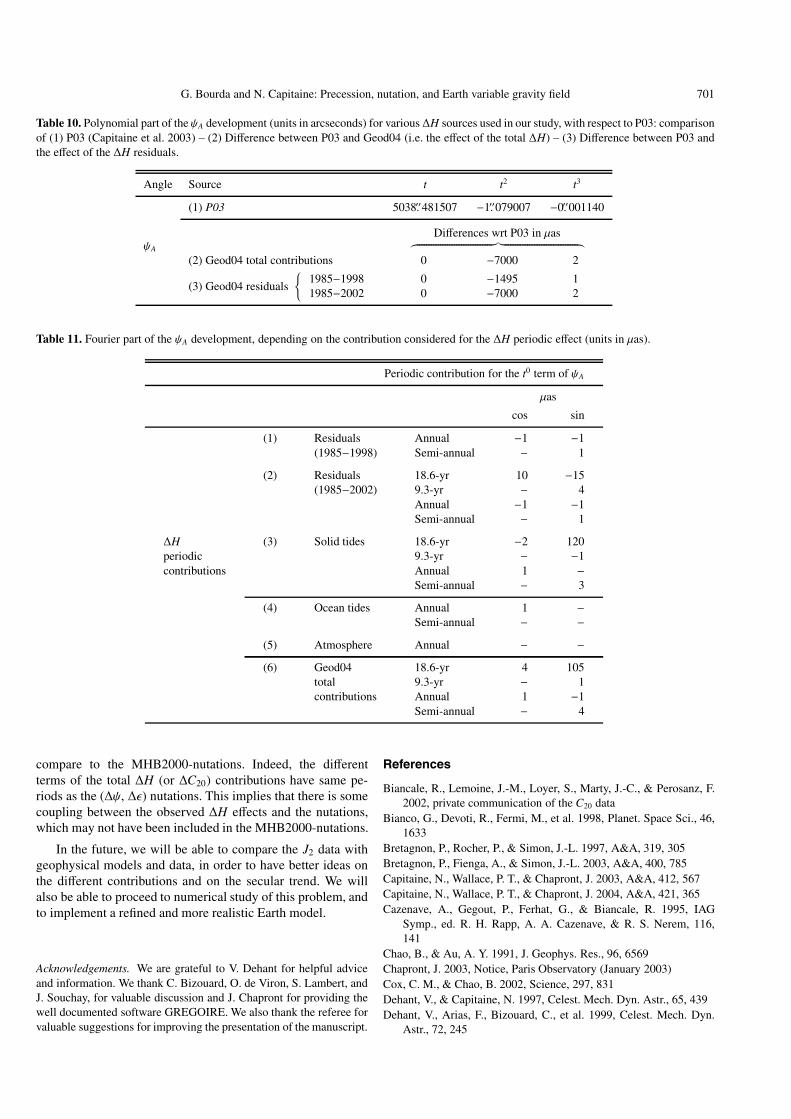
G. Bourda and N. Capitaine: Precession, nutation, and Earth variable gravity field 701
Table 10. Polynomial part of theψA development (units in arcseconds) for various ∆H sources used in our study, with respect to P03: comparisonof (1) P03 (Capitaine et al. 2003) – (2) Difference between P03 and Geod04 (i.e. the effect of the total ∆H) – (3) Difference between P03 andthe effect of the ∆H residuals.
Angle Source t t2 t3
(1) P03 5038.′′481507 −1.′′079007 −0.′′001140
ψA
Differences wrt P03 in µas︷︸︸︷
(2) Geod04 total contributions 0 −7000 2
(3) Geod04 residuals
1985−19981985−2002
00
−1495−7000
12
Table 11. Fourier part of the ψA development, depending on the contribution considered for the ∆H periodic effect (units in µas).
Periodic contribution for the t0 term of ψA
µas
cos sin
(1) Residuals Annual −1 −1(1985−1998) Semi-annual − 1
(2) Residuals 18.6-yr 10 −15(1985−2002) 9.3-yr − 4
Annual −1 −1Semi-annual − 1
∆H (3) Solid tides 18.6-yr −2 120periodic 9.3-yr − −1contributions Annual 1 −
Semi-annual − 3
(4) Ocean tides Annual 1 −Semi-annual − −
(5) Atmosphere Annual − −(6) Geod04 18.6-yr 4 105
total 9.3-yr − 1contributions Annual 1 −1
Semi-annual − 4
compare to the MHB2000-nutations. Indeed, the differentterms of the total ∆H (or ∆C20) contributions have same pe-riods as the (∆ψ, ∆ε) nutations. This implies that there is somecoupling between the observed ∆H effects and the nutations,which may not have been included in the MHB2000-nutations.
In the future, we will be able to compare the J2 data withgeophysical models and data, in order to have better ideas onthe different contributions and on the secular trend. We willalso be able to proceed to numerical study of this problem, andto implement a refined and more realistic Earth model.
Acknowledgements. We are grateful to V. Dehant for helpful adviceand information. We thank C. Bizouard, O. de Viron, S. Lambert, andJ. Souchay, for valuable discussion and J. Chapront for providing thewell documented software GREGOIRE. We also thank the referee forvaluable suggestions for improving the presentation of the manuscript.
References
Biancale, R., Lemoine, J.-M., Loyer, S., Marty, J.-C., & Perosanz, F.2002, private communication of the C20 data
Bianco, G., Devoti, R., Fermi, M., et al. 1998, Planet. Space Sci., 46,1633
Bretagnon, P., Rocher, P., & Simon, J.-L. 1997, A&A, 319, 305Bretagnon, P., Fienga, A., & Simon, J.-L. 2003, A&A, 400, 785Capitaine, N., Wallace, P. T., & Chapront, J. 2003, A&A, 412, 567Capitaine, N., Wallace, P. T., & Chapront, J. 2004, A&A, 421, 365Cazenave, A., Gegout, P., Ferhat, G., & Biancale, R. 1995, IAG
Symp., ed. R. H. Rapp, A. A. Cazenave, & R. S. Nerem, 116,141
Chao, B., & Au, A. Y. 1991, J. Geophys. Res., 96, 6569Chapront, J. 2003, Notice, Paris Observatory (January 2003)Cox, C. M., & Chao, B. 2002, Science, 297, 831Dehant, V., & Capitaine, N. 1997, Celest. Mech. Dyn. Astr., 65, 439Dehant, V., Arias, F., Bizouard, C., et al. 1999, Celest. Mech. Dyn.
Astr., 72, 245

702 G. Bourda and N. Capitaine: Precession, nutation, and Earth variable gravity field
de Viron, O. 2004, private communicationDickey, J. O., Marcus, S. L., De Viron, O., & Fukumori, I. 1975,
Science, 298Farrell, W. E. 1972, Rev. Geophys. Space Phys., 10, 761Fukushima, T. 2003, Astr. J., 126, 494Gegout, P., & Cazenave, A. 1993, Geophys. Res. Let., 18, 1739Kinoshita, H. 1977, Celest. Mech., 15, 277Lambeck, K. 1988, Geophysical geodesy: The Slow Deformations of
the Earth, Oxford Science PublicationsLambert, S., & Capitaine, N. 2004, A&A, 428, 255Lieske, J. H., Lederle, T., Fricke, W., & Morando, B. 1977, A&A,
58, 1
Mathews, P. M., Herring, T. A., & Buffett, B. A. 2002, J. Geophys.Res., 107, B4
McCarthy, D. D. 1996, IERS Conventions, 21, Observatoire de Paris,Paris
Morrison, L., & Stephenson, R. 1997, Contemporary Physics, 38, 13Nerem, R. S., Chao, B. F., Au, A. Y., et al. 1993, Geophys. Res. Let.,
20, 595Souchay, J., & Kinoshita, H. 1996, A&A, 312, 1017Souchay, J., & Folgueira, M. 1999, Earth, Moon and Planets, 81, 201Williams, J. G. 1994, AJ, 108 (2), 711Yoder, C. F., Williams, J. G., Dickey, J. O., et al. 1983, Nature, 303,
757


![G. Bourda and N. Capitaine arXiv:0711.4575v1 [astro-ph] 28 ... · G. Bourda and N. Capitaine: Precession, nutation, and Earth variable gravity field 3 Hence, the link between the](https://static.fdocuments.in/doc/165x107/5f39dedd612672101e3e6355/g-bourda-and-n-capitaine-arxiv07114575v1-astro-ph-28-g-bourda-and-n.jpg)