Precautionary Savings with Risky Assets:

When Cash is Not Cash

Ran Duchin, Thomas Gilbert, Jarrad Harford, and Christopher Hrdlicka*

June 2015

ABSTRACT

We show that U.S. industrial firms invest heavily in non-cash, risky financial assets such as corporate debt, equity, and mortgage-backed securities. Risky assets represent 40% of firms’ investment portfolios, or 6% of total book assets. They are concentrated in financially unconstrained firms, with large investment portfolios, and low demand for precautionary savings. We assess the optimality of risky investments and find that they are undertaken by poorly-governed firms and discounted by 13-22% compared to safe investments. We conclude that this activity represents an unregulated asset management industry of more than $1.5 trillion, which questions the traditional boundaries of nonfinancial firms.

JEL classification: G32, G34

Keywords: Cash, Liquidity, Reserves, Investment Securities, Risk, SFAS 157, Fair Value, Taxes

                                                            *  All authors are at the Michael G. Foster School of Business at the University of Washington. Email:

duchin@uw.edu; gilbertt@uw.edu; jarrad@uw.edu; hrdlicka@uw.edu. We are grateful to two anonymous referees, Michael Roberts (the editor), David Cordova (tax partner at Deloitte), Harry DeAngelo, Dave Denis, Amy Dittmar, Mike Faulkender, Laurent Fresard, Ron Giammarino, Todd Gormley, Jay Hartzell, Carolin Pflueger, Lee Pinkowitz, Bill Resler, Martin Schmalz, Terry Shevlin, Jake Thornock, and Jeff Zwiebel for insightful discussions and comments. We thank Aaron Burt, Harvey Cheong, Matthew Denes, John Hackney, Lucas Perin, and especially Rory Ernst for excellent research assistance. We also thank seminar participants at Carnegie Mellon, City University-Hong Kong, Emory University, Erasmus University, the Interdisciplinary Center Herzliya (IDC), the University of Amsterdam, the University of Copenhagen, the University of Hong Kong, the University of Kentucky, the University of Utah, Tilburg University, Tulane University, Washington University in St. Louis, and the participants of the ASU Sonoran Winter Finance Conference 2014, the 9th Annual FIRS meetings, the 2014 SFS Cavalcade, the Pacific Northwest Finance Conference, the 2014 LBS Summer Finance Symposium, and the 2014 Western Finance Association Meetings for helpful comments.

USC FBE FINANCE SEMINARpresented by: Jarrad Harford

Friday, Oct. 2, 201510:30 am - 12:00 pm; Room: JKP-102

  

1. Introduction

A key assumption in studies of corporate cash holdings is that industrial firms invest in actual

cash or risk-free, near-cash securities. Recent anecdotal evidence in the press, however, suggests

that corporate treasuries have considerably broadened the scope of securities in which they

invest. For example, the article “Google’s Latest Launch: Its Own Trading Floor,” published in

Business Week on May 27, 2010, reports that: “Google, it turns out, has launched a trading floor

to manage its $26.5 billion in cash and short-term investments… One of the company's goals is

to improve the returns on its money, which until now has been managed conservatively.”

In this paper we investigate the composition, determinants, and implications of financial

assets held by nonfinancial firms. We show that firms hold large portfolios, which comprise a

wide range of financial assets. Apple, for example, holds $121 billion, or 70% of its book assets,

in financial assets, placing it among the largest hedge funds in the world. Collectively, the firms

in our sample manage over $1.5 trillion in financial assets. Despite the similarity to the

traditional asset management industry, the regulation and disclosure requirements of this shadow

asset management industry are minimal.

Our empirical analysis exploits the implementation of the Statement of Financial

Accounting Standards (SFAS) No. 157 in 2009, which requires all firms to report the fair-value

measurement of major asset classes on their balance sheet.1 We focus on firms’ non-operating

financial assets that comprise the balance sheet accounts ‘cash and cash equivalents’, ‘short-term

investments’, and additional assets reported as ‘long-term investments’ or ‘other assets’, which

were not considered by prior studies of cash holdings.2 We hand-collect detailed data on the asset

classes that constitute firms’ total financial asset portfolios from the footnotes of annual reports

for all industrial firms in the S&P 500 Index from 2009 to 2012.

Our findings shed new light on both the size and the composition of industrial firms’

                                                            1 See paragraph 32 of SFAS No. 157, paragraph 19 of SFAS No. 115, and Appendix A for more information. 2 We exclude restricted assets, pension assets and deferred executive compensation since they can be viewed as

operating assets invested in a particular project or labor payments. We also exclude derivative hedging, which is studied extensively in a separate literature (e.g., Guay and Kothari, 2003, and Jin and Jorion, 2006). 

1

  

financial assets. First, we find that the total value of the firm’s financial asset portfolio is 24.6%

larger than the traditional measure of corporate cash holdings. This difference stems from the

inclusion of long-term financial assets. Critically, the existing cash literature implicitly ignored

these financial assets, which are held to fund real investment opportunities and mitigate adverse

shocks that may arise in the more distant future.

Second, our estimates indicate that firms invest heavily in non-cash securities that are

both risky and illiquid. We show that risky securities represent 38.3% of aggregate asset

portfolios, or 5.8% (5.6%) of the aggregate book value (market value of equity) of industrial

firms in the S&P 500 Index. The vast majority of risky securities (roughly 79%) are also illiquid.

They include a wide array of securities, such as corporate debt (23.6%), equity (8.6%), asset-

backed or mortgage-backed securities (8.4%), government debt excluding U.S. Treasuries

(15.3%), and ‘other securities’, both domestic and foreign. In contrast, safe assets, which

represent 61.7% of aggregate portfolios, comprise money-like securities with minimal risk and

illiquidity: time deposits, bank deposits, money market funds, commercial paper, and U.S.

Treasury securities.

To guide our exploration of the factors driving this behavior, we present a unified

conceptual framework that models the marginal benefits and costs of investing in risky or illiquid

financial assets. Our baseline model shows that financially constrained firms or those with high

demand for precautionary savings should never invest in risky financial assets. Unconstrained

firms are, at best, indifferent to the composition of their asset portfolio. When we introduce

considerations of corporate and personal taxes (domestic and foreign), the conclusions are less

clear-cut. While in some cases, taxes provide an incentive to invest in risky financial assets, the

bottom line is that taxes provide neither a clear advantage nor disadvantage to doing so. Finally,

we show that agency conflicts and managerial attributes such as risk tolerance or overconfidence,

can tip the balance toward investing in risky financial assets.

Our empirical findings are consistent with the predictions of our theory. We find that

risky investments increase substantially as the firm becomes more financially unconstrained and

2

  

holds a larger asset portfolio. Our univariate estimates indicate that firms in the lowest portfolio

size quintile invest 9.9% of their portfolio in risky securities, whereas firms in the top quintile

invest 39.7% of their portfolio in risky securities. We find similar results in multivariate

regressions. To mitigate endogeneity concerns about the joint determination of the size and

composition of the asset portfolio, we provide estimates from a two stage least squares (2SLS)

model, which exploits unexpected operating cash flow innovations. Our 2SLS estimates suggest

that an increase of one percentage point in the size of the asset portfolio leads to an increase of

30 basis points in the fraction of the portfolio invested in risky assets.

Having established the link between the size of the asset portfolio and its composition,

we turn to investigate the effects of additional firm-level and manager-level attributes. Our

estimates reveal a number of systematic patterns. First, consistent with Opler et al. (1999) and

Bates et al. (2009), the size of the asset portfolio increases in firm-level proxies for the demand

for precautionary savings, such as cash flow volatility, investment opportunities, and firm size.

In contrast, holding constant the size of the asset portfolio, risky financial investments are

concentrated in large, low cash-flow volatility firms, with only average investment opportunities.

These findings are consistent with the prediction that more financially constrained firms, with a

stronger precautionary savings motive, will avoid risky financial assets.

Second, in the analysis of taxes, we consider pre-tax levels of domestic and foreign

earnings, coupled with several measures of the tax costs of repatriating foreign earnings. Our

results indicate that firms with higher tax costs hold larger portfolios of financial assets,

consistent with the evidence in Foley et al. (2007) and Faulkender and Petersen (2012).

However, we find that tax costs do not help us understand the allocation of those assets across

safe and risky securities. In Appendix C, we present detailed theoretical analyses suggesting that

in most jurisdictions, the differential tax rates do not provide incentives to invest in risky assets.

Third, we find evidence that poorly governed firms invest more in risky financial assets.

Following Dittmar and Mahrt-Smith (2007), we measure the quality of corporate governance

using the E-index (Bebchuk et al., 2009, based on Gompers et al., 2003), institutional block

3

  

holdings, and pension fund holdings. Our estimates indicate that a decrease of one standard

deviation in the quality of governance is associated with an increase of 1.2-2.2% in risky

investments. This evidence is consistent with the hypothesis that the manager may derive private

benefits from investing in risky assets because it makes her job more interesting or helps develop

human capital that can be valuable elsewhere (e.g., in the asset management industry).

Fourth, we find that proxies for managerial overconfidence are associated with larger

risky investments, consistent with managers’ belief that they are benefiting themselves and

shareholders by “putting their money to work” and generating positive alphas. We also find that

increased managerial risk-taking preferences, measured by option-based compensation and

gender, are associated with more risky investments.

Fifth, we consider the possibility that firms consistently generate positive alphas from

risky investments. The large literature on the inability of professional money managers to earn

positive abnormal returns after fees (see Fama and French, 2010, and references therein),

however, makes it unlikely that corporate managers are able to do so. The poor disclosure

requirements surrounding firms’ financial assets do not allow us to measure their returns directly.

Thus, to assess whether there is any net value creation from investing in risky securities, we

measure the marginal value to shareholders of risky investments and investigate how firms

finance these investments. We find that the value of a marginal dollar invested in risky securities

is 12.9% to 21.5% lower than if it were invested in safe securities. In addition, we find that firms

finance risky investments from operating cash flows. In contrast, they invest funds from external

financing in safe securities. Since industrial firms are unable to obtain financing to invest in risky

financial assets, we conclude that there is little support that their performance as a financial

intermediary is value-creating for shareholders.

Our paper is related to two recent studies by Cardella, Fairhurst, and Klasa (2015) and

Brown (2014). These papers use Compustat data to investigate the properties of corporate cash

holdings. We complement these papers in two important ways: (1) we study the asset

composition of a firm’s entire asset portfolio, including financial assets outside the standard

4

  

Compustat-based measure of cash holdings; and (2) we study detailed asset allocations rather

than aggregate data. Thus, our empirical approach allows us to study firm-specific portfolio

allocation across various dimensions such risk and illiquidity.

More broadly, our results have implications for the literature on corporate cash holdings,

as they challenge the dominance of the precautionary savings motive for an economically

significant portion of firms’ perceived “cash” holdings (see, for example, Lins et al., 2010). They

are also relevant for the debate over whether and when cash should be returned to shareholders

through a change in payout policy. In addition, since undrawn lines of credit cannot be invested

in risky assets, they point to a further dimension on which lines of credit and cash holdings differ

(see, for example, Sufi, 2009, Disatnik et al., 2013, and Acharya et al., 2013).

Overall, our findings open new questions into the explanations for, and policy

implications of, what are essentially hedge funds operating within non-financial firms. An

investment company managing more than $100 million of other people’s money is heavily

regulated and faces disclosure requirements around its holdings and performance. In contrast,

U.S. industrial companies manage more than $1.5 trillion on behalf of their shareholders, with

very minimal disclosure requirements. Thus, shareholders can neither assess the strategy and

performance of this growing shadow asset management industry, nor adjust the rest of their

portfolio appropriately.

The remainder of the paper proceeds as follows. In Section 2 we discuss our data and

classification methods. In Section 3 we provide detailed evidence on the risk and illiquidity

composition of firms’ financial asset portfolios. In Section 4 we outline a theoretical framework

for understanding the benefits and costs of investing in risky or illiquid financial assets. Section 5

investigates the determinants of the composition of firms’ asset portfolios. Section 6 examines

the value of risky assets. Section 7 gives provides concluding remarks.

5

  

2. Data and Classification

2.1 Sample Selection and Financial Asset Data

We hand-collect data on firms’ financial assets from the footnotes of annual reports (10-K)

available on the Securities and Exchange Commission’s Edgar database. The Statement of

Financial Accounting Standards (SFAS) No. 157, implemented in 2009, requires firms to

disclose the process used to calculate the fair value of their assets. Most firms report this

information in a footnote labeled “fair value measurements.”

Our sample includes all firms that have been members of the S&P 500 Index at any point

between 2009, the year in which SFAS No. 157 became effective, and 2012, the most recent year

for which data were available when we collected the data. Following the literature, we drop all

financial firms (SIC 6000-6999) and regulated utilities (SIC 4900-4999). Our final sample

includes 446 firms and 1,727 firm-year observations spanning four fiscal years.3 We obtain

monthly stock returns from CRSP and all other firm-level accounting data from Compustat.

We focus on firms’ non-operating financial assets, which comprise the balance sheet

accounts ‘cash and cash equivalents’, ‘short-term investments’, and additional assets reported as

‘long-term investments’ or ‘other assets’. We exclude restricted assets, pension assets and

deferred executive compensation since they can be viewed as operating assets invested in a

particular project or labor payments. We also exclude derivative hedging, which is studied in a

separate literature (e.g., Guay and Kothari, 2003, and Jin and Jorion, 2006).

It is useful to compare the asset portfolio that we study to the traditional measure of cash

holdings, defined as the sum of the balance sheet accounts ‘cash and cash equivalents’

(Compustat item CH) and ‘short-term investments’ (Compustat item IVST). These accounts

include financial assets with maturity of up to 90 days at issuance, and financial assets that the

                                                            3 We exclude the payroll processing firms ADP and Paychex since they behave as financial firms and hold large

amounts of deposits on behalf of their customers. 

6

  

firm intends to liquidate within a year, respectively. In contrast, we identify the firm’s entire

portfolio of financial assets, which typically includes additional financial assets outside ‘cash and

cash equivalents’ and ‘short term investments’, held in the balance sheet accounts ‘long-term

investments’ and ‘other assets’.4

Importantly, firms can hold similar financial assets across these different accounts. In

particular, ‘short term investments’, ‘long term investments’, and ‘other assets’ all include

financial assets such as corporate bonds, stocks, and mortgage-backed securities. The only

distinction is the firm’s intention to liquidate some positions within a year and hold on to the

others for more than a year. Therefore, one conclusion that we draw from our data collection

process is that the standard approach to measuring corporate cash holdings implicitly assumes

that cash holdings are held for no more than a year. We believe that the previous cash literature

has not recognized this limitation. Our estimates indicate that compared to the standard measure

of cash holdings, which only includes financial assets held in ‘cash and cash equivalents’ and

‘short term investments’, the total amount of financial assets held by corporations is 25% larger.

2.2 Asset Classification

Our hand-collected data allow us to group similar financial assets across different balance sheet

accounts. Specifically, our approach is to sort the firm’s financial assets based on their asset

classes, irrespective of the balance sheet account in which they are reported. We further

distinguish financial asset classes along two dimensions: illiquidity and risk. We defer a more

formal treatment of illiquidity and risk to Section 4, which presents our theoretical framework.

Here, we provide an intuitive description of our classification method.

To measure asset illiquidity, we exploit the requirement in SFAS No. 157 to report each

                                                            4 Note that while ‘cash and cash equivalents’ and ‘short-term investments’ only include financial assets, ‘long-term

investments’ and ‘other assets’ include both financial and non-financial assets.

7

  

asset as level 1, 2, or 3, based on the inputs necessary to assess its fair value. Level 1 includes

assets with quoted prices in active markets for identical assets; examples are equities and on-the-

run U.S. Treasury bonds. Level 2 includes assets without quoted prices in active markets, where

other observable inputs are required; examples are municipal bonds and other fixed income

securities that trade in over-the-counter markets. Level 3 includes the remaining assets where

other unobservable inputs are required; examples are auction rate securities and Greek bonds

(Milbradt, 2012). We use the asset level breakdown to measure asset illiquidity, since higher

levels represent greater difficulty in calculating the current fair value of a given asset.

While we would like a continuous measure of risk, we are unable to produce one because

firms only disclose broad financial asset classes, such as government bonds, corporate bonds,

equities, etc. We therefore employ a dichotomous classification scheme into safe and risky

assets. An advantage of this broad classification scheme is that it mitigates measurement issues

that may arise due to perverse situations where, for example, a junk bond fund has more

systematic risk than a conservatively invested equity fund. More specifically, safe assets

comprise money-like securities with minimal risk, which the Federal Reserve labels M4 (and L):

cash, cash equivalents, time deposits, bank deposits, money market funds, commercial paper, and

U.S. Treasury securities. The money-like nature of these safe assets fits closely with the existing

literature’s implicit assumption about the nature of corporate “cash” holdings.

We recognize that there is no absolutely risk-free security, and, in particular, that our safe

assets may include interest rate and inflation risk. However, the magnitude of these risks, as well

as the risk premia they earn, are small compared to the risk exposures of the remaining assets,

which we classify as risky: corporate debt, equity, asset- and mortgage-backed securities,

government debt excluding U.S. Treasuries, and other securities.

Figure 1 presents a Venn diagram that sketches the asset breakdown by balance sheet

accounts, risk, and illiquidity. Figure 1 shows that contrary to the common view, firms may hold

8

  

risky or illiquid assets in the balance sheet accounts ‘cash and cash equivalents’ and ‘short-term

investments’. Further, firms may hold additional financial assets in other accounts, including

‘long-term investments’ and ‘other assets’, which can be either safe or risk, and liquid or illiquid.

In the next section, we provide a detailed description of the composition of corporate financial

assets based on asset classes, risk, and illiquidity.5

3. The Composition of Corporate Financial Assets

In this section, we investigate the asset composition of firms’ financial assets. For each category

and asset class, Panel A of Table I shows the fair dollar value and the fair value normalized by

total book assets (AT), market value of equity, the standard Compustat-based measure of cash

holdings (CHE), and total financial investments. These ratios adjust for the scale of the firm and

its investments, thus facilitating the comparison of our results to the existing literature. Here, we

report aggregate sample-wide values for 2012, the most recent year in our sample. We provide

analogous equally-weighted statistics in Appendix B, Table B.1.

Panel A shows that firms hold a substantial percentage of their financial investments in

risky assets. Specifically, the total value of risky assets held by our sample firms in 2012 was

$611 billion, collectively accounting for 5.8% of total book assets and 5.6% of the market value

of equity. Aggregated across all our sample firms, the value of risky investments is 38.3% that of

total investments. These estimates are very similar across the other years in our sample.

We are also interested in comparing our estimates of firms’ total financial investments to

the standard measure of cash holdings in the literature, which comprises ‘cash and cash

equivalents’ and ‘short-term investments’ (Compustat data item CHE). Our estimates indicate

that the value of risky investments is 47.8% that of CHE. Furthermore, total financial

investments are 24.6% larger than CHE.

                                                            5 In Appendix A, we provide additional details about our collection and classification process, including illustrations

of firms’ financial asset reporting.

9

  

More granularly, firms invest heavily in debt securities. Panel A shows that 2.3% of firm

value is invested in non-Treasury government debt, including municipal and agency debt; about

1.6% is invested in corporate debt; and more than 0.7% is invested in other debt securities, with

the majority invested in asset-backed and mortgage-backed securities. Firms also invest about

1.1% in other securities, including 0.3% in equity securities. The majority of corporate financial

investments are held in domestic securities. In fact, foreign security holdings are negligible for

all asset classes but government debt, where they amount to 0.6% of aggregate assets.

Panel B of Table I shows how assets are classified by asset levels. Asset levels are

measures of liquidity since they are determined by the type of inputs required to assess the fair

value of the asset: quoted prices in active markets for identical assets (level 1), significant other

observable inputs (level 2), or significant other unobservable inputs (level 3). Thus, level 1 assets

are the most liquid and level 3 assets are the most illiquid. It is clear from the panel that firms

hold some assets that are very illiquid (level 3), and that liquidity and risk are different.

Taken together, the estimates in this section suggest that firms invest heavily in risky and

illiquid financial assets, and moreover, that financial assets are substantially larger than

traditional measures of cash holdings. In Appendix B, Table B.2, we provide additional

descriptive analyses of the industry-level breakdown of financial asset holdings (Panels A and

B), and list the 20 largest holders of risky assets (Panel C). Firms in the technology and

healthcare sectors hold more risky financial assets on average, and represent most of the top-20

list. We therefore control for industry effects in subsequent analyses. In the next section, we

develop a theoretical framework to guide our analysis of the determinants and implications of

financial asset holdings.

10

  

4. Theoretical Framework

The existing literature identifies various motives for the amount of corporate “cash” holdings but

is generally silent about the composition of these holdings. The implicit assumption is that these

holdings comprise cash or near-cash securities, i.e., liquid and virtually risk-free financial assets.

As the prior section shows, in reality firms’ portfolios are more complex. We examine how the

marginal benefits and costs of financial assets vary with their amount and composition, taking

into account non-mutually exclusive forces such as precautionary demand, taxes, and agency

conflicts. Our framework extends the standard cash model as in Kim et al. (1998), Duchin

(2010), Almeida et al. (2004) and Almeida et al. (2014) by showing how the marginal benefits of

financial assets vary with their composition. It also builds on the intuition inherent in the optimal

portfolio choice problem solved by Gilbert and Hrdlicka (2015) where universities face the

trade-off between real investment projects and the size and allocation of their ‘precautionary

savings’ (i.e., their endowments).6 Importantly, to study the risk-composition of a firm’s

financial assets, we consider risk-averse investors rather than the risk-neutral investors studied in

prior literature.

4.1 Definitions: financial assets, liquidity, and risk

Absent capital market frictions, the firm does not need to hold assets internally, and if it were to

hold assets, it would be indifferent to their composition.7 When external financing frictions do

exist, the firm cannot instantaneously and costlessly access additional capital. It therefore holds

additional assets internally for future use. These additional assets are precautionary savings,

which could take any form, including operating assets that the firm can liquidate to meet its

                                                            6 Dynamic models of the value of cash holdings include Decamps et al. (2011), Bolton et al. (2011), Hugonnier et

al. (2015) and references therein. 7  We assume that financial markets are perfectly competitive such that any individual firm behaves as a price taker. 

11

  

future needs. In practice, illiquidity, one form being transaction costs, makes the firm hold non-

operating financial assets instead. We focus exclusively on these non-operating financial assets.

Illiquidity also influences the type of non-operating financial assets that the firm uses as

precautionary savings. On the one hand, holding liquid assets is beneficial because they can be

converted fairly readily to cash with little or no loss of principal. On the other hand, with

increasing illiquidity comes the benefit of increasing interest (see Azar et al., 2015, for an

analysis of the changing cost of carry for liquid holdings). Importantly, this interest is

compensation for illiquidity, not risk, and is called a liquidity premium (see Opler et. al., 1999).

There is a range of safe assets, classified by the Federal Reserve in a decreasing order of liquidity

(M0 through M4 and L): cash, demand deposits, money market funds, time deposits, commercial

paper, Treasury Bills, and Treasury Notes and Bonds (Anderson and Kavajecz, 1994).

Our focus, however, is on the risk in the composition of financial assets. By risk we mean

systematic risk and for the remainder of the paper, we use the term risk to refer to systematic

risk. We do not separately model or empirically investigate idiosyncratic risk since the firm gains

no benefit from holding a poorly diversified portfolio of financial assets and the available data do

not allow us to measure the idiosyncratic risk of firms’ holdings.

Just as more illiquid assets earn a higher (risk-free) interest rate, riskier securities earn a

higher expected return. Sources of this risk premium include market risk, size, book-to-market,

and momentum, among others. Importantly, one systematic risk factor is liquidity risk (e.g.,

Pastor and Stambaugh, 2003, and Sadka, 2006). However this liquidity risk factor is different

from the illiquidity level of a security previously discussed. Liquid stocks, for example, can have

high liquidity risk exposure (Sadka, 2014). Moreover, there exist securities with various

combinations of liquidity and risk. For instance, equities are highly liquid but risky, whereas off-

the-run Treasury Bonds are relatively illiquid but safe. This point is illustrated in Appendix B,

Figure B.1, which illustrates the risk-illiquidity combinations that correspond to various financial

12

  

assets. Next, we use these definitions to model the effects of risk and illiquidity on the marginal

benefits and costs of holding financial assets.

4.2 Baseline marginal benefits and costs

Our baseline model follows the standard cash model in the literature (e.g., Duchin, 2010, and

Almeida et al., 2004 and 2014). In the model, the cost of holding financial assets is forgoing

positive NPV real investment opportunities today, and the benefit is being able to continue

current projects or undertake new projects despite negative cash flow shocks. The decreasing

marginal productivity of the firm’s real investment technologies implies that the marginal cost of

holding financial assets increases in the amount of financial assets and the marginal benefit

decreases.8

The firm chooses the amount of financial asset holdings to equate the marginal cost and

marginal benefit. Note that if the firm could exhaust all positive NPV projects today or in the

future, then segments of the marginal cost or benefit curves would be zero, creating regions of

indifference (or indeterminacy) for the amount of financial assets (as in Almedia et al., 2014).

To understand the composition of financial assets in this framework, first notice that the

marginal cost does not change with the composition of financial assets because the firm must

forgo the same amount of investments today to produce a dollar of financial asset holdings. The

marginal benefit, however, changes with the composition of financial assets because the type of

financial assets affects the firm’s ability to exploit profitable projects in the future. In the

following subsections, we detail these shifts in the marginal benefit curve to describe the

codetermination of the amount and composition of financial assets.

                                                            8  Firm-level indicators that affect the firm’s marginal benefit curve for financial assets (e.g., precautionary savings)

have been studied extensively in prior literature (see Bates et al., 2009, and Almeida et al., 2014, for reviews). In particular, firms with more volatile cash flows, better investment opportunities, and higher deadweight costs of external finance, have a higher demand for precautionary savings. 

13

  

4.3 The effect of illiquidity

Suppose that the firm’s initial asset allocation comprises financial assets that are both safe and

liquid, and consider a switch to less liquid assets. Such a reallocation has two offsetting effects

on the marginal benefit of financial assets, which are demonstrated in Panel A of Figure 2. On

the one hand, illiquidity increases the marginal benefit of financial assets by producing risk-free

interest as compensation for the illiquidity. On the other hand, if the firm needs capital quickly

and/or unexpectedly, illiquidity impedes the firm’s access to its financial assets, thereby reducing

their marginal benefit. However, illiquidity has little or no effect on the marginal benefit if the

firm only needs access at long predictable horizons. The net of both effects determines whether a

shift to illiquid assets increases the total benefit of holding these assets. Importantly, when the

net marginal benefit increases from illiquidity, the optimal amount of financial assets firms hold

will be higher than if the firm were to hold only liquid assets.

4.4 The effect of risk

Relative to the same initial allocation of safe and liquid financial assets, an increase in risk has

two effects, which are demonstrated in Panel B of Figure 2. The first effect arises due to

investors’ risk aversion and does not impact the marginal benefit of financial assets. While

riskier financial assets yield higher expected returns on the firm’s asset portfolio, risk-averse

investors recognize the increase in the overall risk of the firms, and therefore require a higher

expected return. Thus, the firm’s cost of capital increases to exactly offset the higher expected

returns, leaving the marginal benefit of financial asset holdings unchanged. This zero net effect is

the basic capital structure equation in which the cost of capital is determined by the riskiness of

the firm’s total assets, both real and financial.

Given that the first effect is zero on net, the marginal benefit of risk is determined by the

following effect, which arises from the interaction between: (1) the volatility of risky payoffs, (2)

14

  

the (state-dependent) decreasing marginal productivity of the firm’s real investment

technologies, and (3) the firm’s (state-dependent) financing constraints. In the simplest case,

with a state independent investment technology and a constrained firm, the concavity of

investment technologies implies that the benefit from additional investing due to good returns is

lower than the cost of forgoing investment due to bad returns.

Based on the above analysis, the total effect of increased risk in the firm’s financial asset

portfolio is a decrease in the marginal benefit for financially constrained firms. Coupled with the

unchanged marginal cost, increasing risk in financial assets reduces the firm’s total benefit of

holding financial assets. This, in turn, implies that financially constrained firms will never

choose to invest their financial assets in risky assets. Put differently, to hold risky financial

assets, firms must be financially unconstrained such that their asset portfolio, even when invested

in risky assets, allows them to exhaust their productive projects in all states of the world. Such

unconstrained firms are indifferent to risky asset allocations due to the offsetting effect of the

higher expected returns and the higher cost of capital. Thus, to the extent that financially

unconstrained firms hold larger financial asset portfolios, we should observe a positive relation

between the size of the asset portfolio and risky asset allocation.9

In the remaining subsections, we explore additional forces that either push financially

unconstrained firms off their indifference curve toward risky financial assets or outweigh the

decrease in the marginal benefit for financially constrained firms.

                                                            9 In reality, investment opportunities tend to covary positively with returns. This positive covariation is essentially

the definition of aggregate good times (see Berk, Green and Naik, 1999, and Carlson, Fisher and Giammarino, 2004). The combination of this positive covariation with counter-cyclical financing frictions (e.g., Eisfeldt and Rampini, 2006, Brown and Petersen, 2011, and Eisfeldt and Muir, 2014) is a decrease in the marginal benefit of financial assets as a result of investing in risky financial assets.

15

  

4.5 The effect of taxes

The current tax code creates a wedge between the after-tax investment income that a shareholder

receives by investing on her own and the after-tax investment income the shareholder receives if

a U.S. C-corporation invests on her behalf. This wedge implies that the higher returns from a

riskier allocation of financial assets may not be exactly offset by the increase in the firm’s cost of

capital. Importantly, the sign and magnitude of this wedge varies with both the type of the

security and the form of the investment gain (e.g., capital gains vs. dividends). In Appendix C,

we present a detailed analysis that explores the tax implications of investing domestic and

foreign balances in financial assets. Table C.1 shows the Federal tax treatment of prevalent risky

securities and gain types for both corporations and individuals.

In general, the net marginal benefit of riskier asset allocations increases when the

corporation has a lower tax rate than the individual’s tax rate on a given security or gain type

(e.g., U.S. equity dividends). When the tax rates are equivalent, the marginal benefits does not

change (e.g., interest payments from fixed income securities). And when the corporation faces a

higher tax rate than the individual investor, the net marginal benefit decreases (e.g., equity and

fixed income long-term capital gains). Importantly, securities do not come in arbitrary

combinations of their potential sources of gains (cash flows vs. returns). It is thus overly

simplistic to view investors (and corporations) as having the option of increasing risk in a

financial security by exclusively increasing expected gains in one particular form, say dividends,

without an increase in returns.10 Therefore, taxes can motivate firms to invest in particular

securities with favorable combinations of cash flows and capital gains, but they do not favor

generically riskier financial assets.

                                                            10 For example, dividend-paying value stocks tend to be riskier than non-dividend paying growth stocks. However,

characterizing all the feasible combinations of cash flow and capital gain return splits is beyond the scope of this work. 

16

  

A multinational firm enjoys an additional tax advantage that may increase the net

marginal benefit of risky asset allocations. In particular, firms can defer paying the difference

between the U.S. tax rate and the foreign tax rate on foreign earnings until they are repatriated.11

This tax advantage, however, is limited to the earnings that serve as the principal for financial

investments, and does not apply to gains from financial investments, which qualify as Subpart F

income and are taxed immediately. The immediate taxation of foreign investment earnings mutes

the (non-uniform) incentives to take risk with foreign financial assets (see Appendix C for

details).12

We conclude that tax considerations, including those of multinational firms, do not create

carte blanche incentives to take risk with financial assets.13 Nevertheless, our model allows for

an internal optimum with both safe and risky assets, whose exact allocation depends on the firm-

specific marginal benefits and costs, including financial constraints and tax incentives.

4.6 The effect of managers

In this subsection, we consider the marginal benefits and costs from the manager’s point of view.

We discuss two possible channels: (1) private benefits, and (2) managerial beliefs.

First, the manager may derive private benefits from investing in risky assets because it

makes her job more interesting or helps develop human capital that can be valuable elsewhere

(e.g., in the asset management industry). Such human-capital building, leading to higher external

                                                            11 Repatriation costs have been discussed by Foley et al. (2007), Faulkender and Petersen (2012), and Faulkender

and Smith (2015). These studies show that firms with higher repatriation tax costs hold more “cash.” 12 This argument relies on the assumption that corporate tax rates are constant. If the firm expects tax rates to fall, or

expects a repatriation tax holiday, its incentives to invest in risky assets may increase, as described in Appendix C. 13 We do note, however, that repatriation taxes imply that domestic and foreign-held financial assets are imperfect

substitutes. It is therefore possible that the firm has high marginal benefits and costs for domestic financial assets, but low marginal benefits and costs for foreign-held financial assets (e.g., Yang, 2015, and Harford, Wang and Zhang, 2015). In the extreme, the firm may act as nearly unconstrained with its foreign-held financial assets, therefore making it indifferent to their risk composition. 

17

  

salaries, decouples the manager’s future salary and the returns to investors (Holmstrom, 1999),

thereby lessening the incentives from ex-post settling up in the labor market (Fama, 1980).14

Second, the manager may attempt to maximize shareholder value, but due to mistaken

beliefs, either her own or those of shareholders, she operates as if the marginal benefits of risky

assets are higher than they truly are. The manager may believe that she can generate abnormal

returns from trading financial assets (or by identifying and underpaying asset managers who

can). The manager can also be driven by confusion over the effect of low-yield financial assets

(e.g., money-like securities) on the firm’s ability to meet its cost of capital. This confusion is

similar to the fallacy that debt is a cheap source of capital (Krueger et al., 2011). In the same

vein, the manager (and shareholders) may choose to speculate in financial markets in an attempt

to “juice” profits or “reach for yield.”15 Finally, the manager may underestimate the need for

precautionary savings. In particular, the manager may perceive the firm to be unconstrained due

to free cash flows (Jensen, 1986), high risk-tolerance, or overconfidence about the firm’s

prospects.

4.7 Summary and testable predictions

Overall, our theoretical framework shows that the composition of a firm’s financial assets is

determined by the interaction of non-mutually exclusive forces driven by precautionary demand,

taxes, and managerial attributes. The main implications of this framework are

1. The size of the firm’s financial asset portfolio is positively correlated with asset illiquidity.

                                                            14 Holding risky financial assets may be viewed by shareholders and directors as a lesser agency cost than reckless

spending on large negative NPV mergers and acquisitions (e.g., Harford, 1999, and Hanlon et al., 2014). If markets are efficient, treasury offices are buying risky financial assets at fair prices and thereby earning the assets’ expected rates of return. Moreover allowing management to invest in risky financial assets with impunity may be an efficient outcome if shareholders and boards of directors cannot distinguish ex-ante good real asset purchases from poor ones. 

15 While the manager may be mistaken as to the source of the benefit from reaching for yield, if enough risk is taken, value may actually be created at the expense of bondholders through the standard risk-shifting channel. Furthermore, increasing the risk of the firm’s financial assets may limit any windfall transfers to bondholders that would occur if the firm’s financial assets were held in a way that made the firm safer than originally expected. 

18

  

2. The more unconstrained the firm is, the more it is willing (indifferent) to invest in risky

financial assets. A corollary is that firms with larger portfolios invest more in risky assets.

3. Taxes may push the firm towards certain securities (capital gains vs. interest/dividends), but

do not uniformly push the firm to hold riskier securities.

4. Firms with higher agency costs will invest more in risky financial assets.

5. Firms with more overconfident or risk-tolerant managers will invest more in risky financial

assets.

5. Determinants of Financial Asset Composition

5.1 Univariate evidence

In this section, we present univariate evidence on the link between the size of the firm’s portfolio

of financial investments and its composition. Table II reports sorts of our sample into quintiles

formed on the size of the asset portfolio. The size of the asset portfolio is measured either based

on the total dollar amount of the portfolio or the portfolio’s dollar amount scaled by the value of

the firm’s book assets. For each size quintile, Panel A reports the average fair value of liquid

(level 1) and illiquid (levels 2 and 3) financial assets, and Panel B reports the fair value of safe

and risky financial assets, scaled by either book assets or total financial assets.

We start with the evidence on asset illiquidity reported in Panel A. Our theory predicts

that as the net marginal benefit from illiquidity increases, firms optimally hold larger financial

asset portfolios. Therefore, we should find that portfolio size is positively correlated with asset

illiquidity. Consistent with this prediction, the estimates in Panel A of Table II reveal a strong

monotonic relation between the size of the asset portfolio and the proportion invested in illiquid

securities. Based on the size of the asset portfolio scaled by book assets, firms in the lowest size

quintile invest 4.2% of their financial assets in illiquid assets. Conversely, firms in the highest

size quintile invest 40.6% of their financial assets in illiquid assets. The inferences are the same

19

  

if we sort firms by unscaled dollar amounts of financial assets.

Panel B of Table II provides evidence on asset risk. Our theory predicts that while

financially constrained firms should not invest in risky financial assets, unconstrained firms are

indifferent to risky investments, and therefore, on the margin, may choose to invest more in risky

assets. To test this prediction, we investigate the link between the size and the asset risk of firms’

financial asset portfolios. In our context, the size of the asset portfolio is the most unambiguous

and relevant measure of financial constraints, given that measuring financial constraints is

notoriously difficult (e.g., Kaplan and Zingales, 1997, and Hadlock and Pierce, 2010).

The estimates in Panel B indicate that the size of the asset portfolio is positively and

monotonically related to the proportion invested in risky securities. Based on the size of the asset

portfolio scaled by book assets, firms in the lowest size quintile invest 9.9% of their financial

assets in risky assets, whereas firms in the highest size quintile invest 39.7% of their portfolio

risky assets. These findings continue to hold if we sort firms by unscaled dollar amounts of

financial assets, and are consistent with the predictions of our model. In the next sections, we

offer more formal evidence on the determinants of the firm’s risky financial assets.

5.2 Baseline regression evidence

Next, we present regression evidence explaining the composition of a firm’s financial asset

portfolio. In addition to estimates from an ordinary least-squares (OLS) regression model, we

also provide evidence from a two stage least-squares (2SLS) regression model to mitigate

endogeneity concerns due to the joint determination of the size of the portfolio and its

composition.

The 2SLS model exploits the variation in the size of the portfolio due to unexpected

operating cash flow shocks. In the first stage, we estimate the following model of the firm’s total

investments in financial assets, scaled by the book value of assets:

20

  

1 , , β X ,

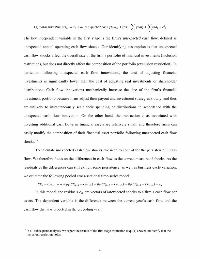
The key independent variable in the first stage is the firm’s unexpected cash flow, defined as

unexpected annual operating cash flow shocks. Our identifying assumption is that unexpected

cash flow shocks affect the overall size of the firm’s portfolio of financial investments (inclusion

restriction), but does not directly affect the composition of the portfolio (exclusion restriction). In

particular, following unexpected cash flow innovations, the cost of adjusting financial

investments is significantly lower than the cost of adjusting real investments or shareholder

distributions. Cash flow innovations mechanically increase the size of the firm’s financial

investment portfolio because firms adjust their payout and investment strategies slowly, and thus

are unlikely to instantaneously scale their spending or distributions in accordance with the

unexpected cash flow innovation. On the other hand, the transaction costs associated with

investing additional cash flows in financial assets are relatively small, and therefore firms can

easily modify the composition of their financial asset portfolio following unexpected cash flow

shocks.16

To calculate unexpected cash flow shocks, we need to control for the persistence in cash

flow. We therefore focus on the differences in cash-flow as the correct measure of shocks. As the

residuals of the differences can still exhibit some persistence, as well as business cycle variation,

we estimate the following pooled cross-sectional time-series model:

In this model, the residuals are vectors of unexpected shocks to a firm’s cash flow per

assets. The dependent variable is the difference between the current year’s cash flow and the

cash flow that was reported in the preceding year.

                                                            16 In all subsequent analyses, we report the results of the first stage estimation (Eq. (1) above) and verify that the

inclusion restriction holds.

21

  

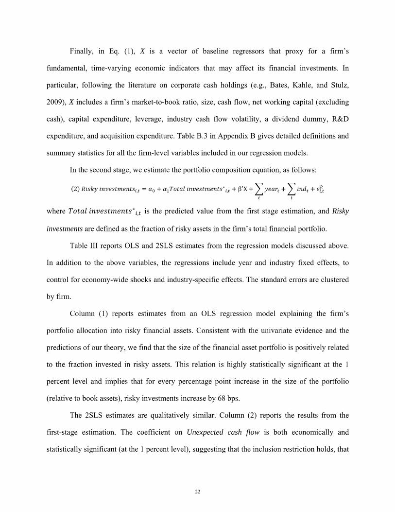
Finally, in Eq. (1), X is a vector of baseline regressors that proxy for a firm’s

fundamental, time-varying economic indicators that may affect its financial investments. In

particular, following the literature on corporate cash holdings (e.g., Bates, Kahle, and Stulz,

2009), X includes a firm’s market-to-book ratio, size, cash flow, net working capital (excluding

cash), capital expenditure, leverage, industry cash flow volatility, a dividend dummy, R&D

expenditure, and acquisition expenditure. Table B.3 in Appendix B gives detailed definitions and

summary statistics for all the firm-level variables included in our regression models.

In the second stage, we estimate the portfolio composition equation, as follows:

2 , ∗, β X ,

where ∗, is the predicted value from the first stage estimation, and Risky

investments are defined as the fraction of risky assets in the firm’s total financial portfolio.

Table III reports OLS and 2SLS estimates from the regression models discussed above.

In addition to the above variables, the regressions include year and industry fixed effects, to

control for economy-wide shocks and industry-specific effects. The standard errors are clustered

by firm.

Column (1) reports estimates from an OLS regression model explaining the firm’s

portfolio allocation into risky financial assets. Consistent with the univariate evidence and the

predictions of our theory, we find that the size of the financial asset portfolio is positively related

to the fraction invested in risky assets. This relation is highly statistically significant at the 1

percent level and implies that for every percentage point increase in the size of the portfolio

(relative to book assets), risky investments increase by 68 bps.

The 2SLS estimates are qualitatively similar. Column (2) reports the results from the

first-stage estimation. The coefficient on Unexpected cash flow is both economically and

statistically significant (at the 1 percent level), suggesting that the inclusion restriction holds, that

22

  

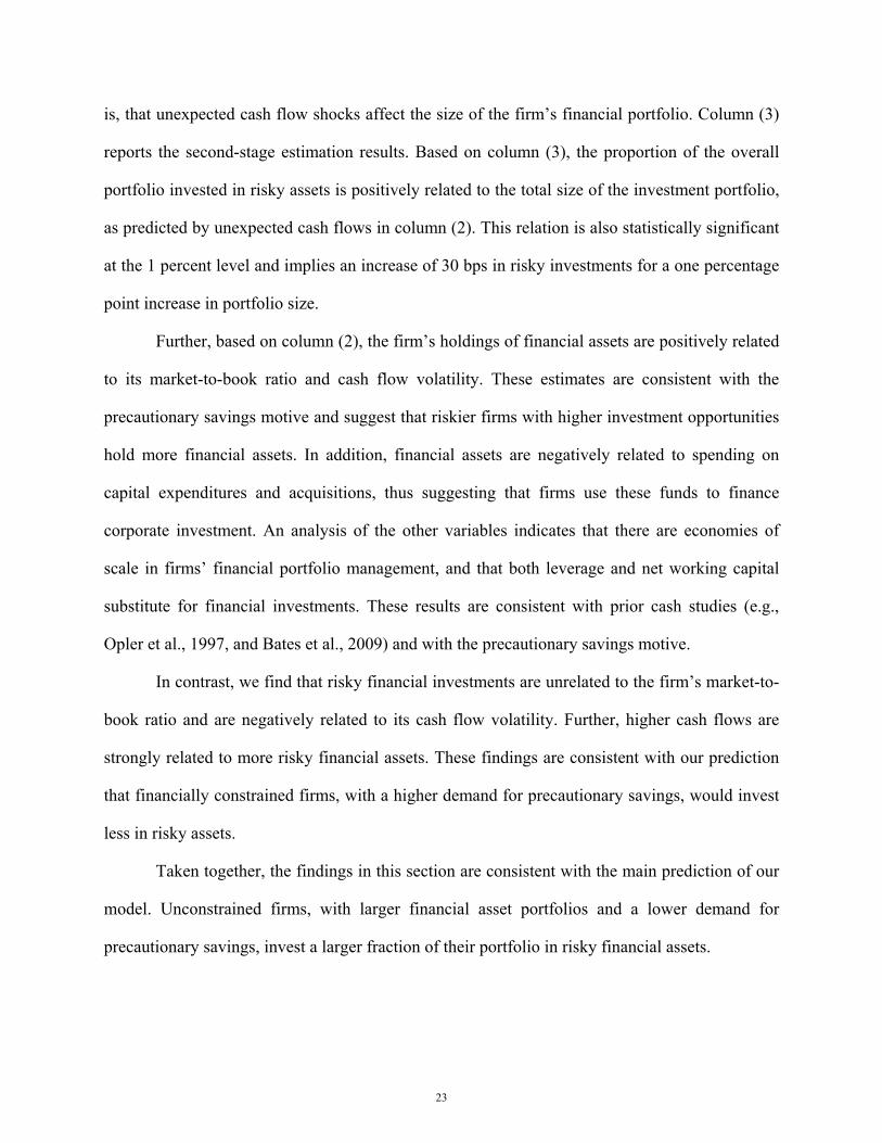
is, that unexpected cash flow shocks affect the size of the firm’s financial portfolio. Column (3)

reports the second-stage estimation results. Based on column (3), the proportion of the overall

portfolio invested in risky assets is positively related to the total size of the investment portfolio,

as predicted by unexpected cash flows in column (2). This relation is also statistically significant

at the 1 percent level and implies an increase of 30 bps in risky investments for a one percentage

point increase in portfolio size.

Further, based on column (2), the firm’s holdings of financial assets are positively related

to its market-to-book ratio and cash flow volatility. These estimates are consistent with the

precautionary savings motive and suggest that riskier firms with higher investment opportunities

hold more financial assets. In addition, financial assets are negatively related to spending on

capital expenditures and acquisitions, thus suggesting that firms use these funds to finance

corporate investment. An analysis of the other variables indicates that there are economies of

scale in firms’ financial portfolio management, and that both leverage and net working capital

substitute for financial investments. These results are consistent with prior cash studies (e.g.,

Opler et al., 1997, and Bates et al., 2009) and with the precautionary savings motive.

In contrast, we find that risky financial investments are unrelated to the firm’s market-to-

book ratio and are negatively related to its cash flow volatility. Further, higher cash flows are

strongly related to more risky financial assets. These findings are consistent with our prediction

that financially constrained firms, with a higher demand for precautionary savings, would invest

less in risky assets.

Taken together, the findings in this section are consistent with the main prediction of our

model. Unconstrained firms, with larger financial asset portfolios and a lower demand for

precautionary savings, invest a larger fraction of their portfolio in risky financial assets.

23

  

5.3 Tax costs of repatriating foreign earnings

In Table IV, we investigate the relation between corporate financial investments and domestic

and foreign income, as well as the tax costs of repatriating earnings. As discussed in Foley et al.

(2007), Compustat data do not provide detailed information about where multinationals have

foreign operations, but it does include information about the levels of foreign income taxes paid

and foreign pre-tax income. These data can be used to compute two measures of the tax cost of

repatriating earnings. The first variable, which we label Tax cost of repatriating earnings, is

computed by first subtracting foreign taxes paid from the product of a firm’s foreign pre-tax

income and its marginal effective tax rate as calculated in Graham (1996). We then scale the

maximum of this difference or zero by total firm assets. To verify that the results are not affected

by the assumptions required to calculate marginal tax rates (Graham, 1996), we also calculate an

alternative tax cost of repatriating earnings using US statutory rates. The Alternative tax cost of

repatriating earnings is computed in the same way as the Tax cost of repatriating earnings, but

with US statutory tax rates used in place of marginal tax rates.

The results in Table IV indicate that while the tax costs of repatriating earnings are

significantly related to the firm’s total financial investments, they are not significantly related to

the composition of financial investments. These findings are consistent with our analysis that the

differential tax rates do not, by themselves, provide an incentive to take risk with financial

investments made in foreign subsidiaries.

Overall, our results are consistent with high repatriation costs incentivizing firms to hold

larger financial asset portfolios (Foley et al., 2007). Consistent with the tax analysis in Appendix

C, however, the larger portfolio size does not generate an incremental incentive to hold foreign

financial assets in risky securities.

24

  

5.4 Agency Theory

In Table V, we investigate the relation between a firm’s financial investment policy and

corporate governance. As discussed in our theory section, risky financial investments may

provide the manager with private benefits by making her job more interesting or helping her

develop human capital. Following Dittmar and Mahrt-Smith (2007), we use the following three

measures of corporate governance: the E-index, the sum of the 5% institutional block holdings,

and the sum of public pension fund holdings.

Consistent with Harford et al. (2008), our first stage regressions suggest that the overall

size of firms’ financial asset holdings is positively related to the quality of corporate governance

(the point estimates are directionally equivalent for all measures of corporate governance, but are

only statistically significant for the E-index). Harford et al. (2008) argue that in poorly governed

firms, managers overinvest, thus reducing the size of the firm’s portfolio.

More importantly, in the second stage regressions we find strong evidence that poor

corporate governance is associated with larger investments in risky financial assets. These

findings hold across all regression models and measures of corporate governance, and are

statistically significant at conventional levels.

The effects are also economically significant. Based on column (3), an increase of one

standard deviation in the E-index is associated with an increase of 2.21% in the portfolio fraction

invested in risky financial assets. Similarly, based on columns (6) and (9), an increase of one

standard deviation in block holdings or pension holdings is associated with an increase of 1.19%

or 1.48% in risky investment, respectively.17

While these results suggest that investing in risky financial assets is potentially driven by

agency conflicts, we caution the reader that risky financial investments can be a lesser agency

                                                            17 A potential concern is that our governance measures are correlated with overseas operations. In unreported results,

we re-estimate the regressions after controlling for pretax foreign income and find similar results.

25

  

cost than reckless spending on large negative NPV mergers and acquisitions. If markets are

efficient, treasury offices are buying risky securities at fair prices, thereby earning the securities’

expected rates of return. Moreover allowing management to invest in risky financial assets with

impunity may be an efficient outcome if shareholders and boards of directors cannot distinguish

ex-ante good real asset purchases from poor ones.

Another shortcoming of our governance measures is that they attempt to measure the

typical characterizations of the agency conflict with a focus on top managers. However, in the

case of risky investments, the agency conflict could be further down in the organization where

treasury personnel prefer to invest in risky assets, either to make their job more interesting or to

develop human capital that can be valuable elsewhere in the asset management industry.

5.5 Managerial Incentives

Next, we investigate the association between CEO overconfidence, compensation contracts, and

firms’ financial investments. As discussed in our theoretical framework, if managers (and

shareholders) believe that investing in risky financial assets is beneficial to equity valuations,

then equity and option compensation, along with overconfidence on the part of managers, could

exacerbate a speculative, reaching-for-yield motivation.

The results are reported in Table VI. While we do not find a significant relation between

a firm’s total financial investments and CEO traits, the results suggest that overconfidence and

stock- and option-based compensation are related to the composition of financial investments.

CEO overconfidence is positively related to the fraction of risky investments. The effect is

statistically significant at the 5 percent level and is economically meaningful: an overconfident

CEO increases the fraction of total investments held in risky financial assets by 1.4%.

Similarly, managers’ stock- and option-based compensation is also positively related to

risky investments. These effects are highly statistically significant at the 1 percent level and are

26

  

also economically significant: an increase of one standard deviation in managers’ stock-based

(option-based) compensation corresponds to an increase of 0.7% (1.35%) in the fraction of total

investments held in risky assets.

An analysis of the other variables reveals that female managers invest less in risky

financial assets. These findings are consistent with the evidence that females are more risk averse

than males (e.g., Byrnes, Miller, and Schafer, 1999, and Eckel and Grossman, 2008). We also

find that age is negatively related to risky investments.

Taken together, these findings support the hypothesis that shareholders and managers

attempt to increase the value of their equity stake by speculating or reaching for yield, possibly at

the expense of the firm’s bondholders.

6. The Value of Risky Investments

We, and presumably investors, would like to be able to directly assess the performance, net of

fees, of firms’ financial asset investments. However, due to limited disclosure requirements, it is

impossible to do so.18 Instead, we assess the net value creation across all motives for investing in

risky financial assets using two methods. First, following Fama and French (1998), Faulkender

and Wang (2006), and Dittmar and Mahrt-Smith (2007), we estimate the marginal value of safe

and risky investments. Second, we investigate the sources of financing for firms’ investments in

risky financial assets. If investing in risky financial assets is sufficiently profitable, firms should

be able to raise external financing to support these investments

In Table VII, we estimate the value of a marginal dollar of cash holdings. Columns 1 and

2 present the Faulkender and Wang (2006) approach, based on the following regression model:

                                                            18 Since the firm’s shares are publicly traded, the alpha from any asset pricing model will not in general be a

measure of the corporate manager’s investment skill. Any expectation of this skill will have been incorporated into the share price immediately upon learning that investing in financial assets is possible.

27

  

, , ΔTotalinvestments , ΔRisky investments , ΔE , ΔNA ,

ΔRD , ΔI , ΔD , Totalinvestments , L , NF ,

Totalinvestments , ΔTotalinvestments ,

L , ΔTotal investments , ,

where , , is a firm’s abnormal return, defined as the stock’s return during the fiscal year

less the return on the matching Fama-French size and book-to-market portfolio, ΔX indicates a

change in X from year t – 1 to t, Ei,t is earnings before extraordinary items, NAi,t is net assets,

RDi,t is R&D Expenses, set to zero if missing, Ii,t is interest expenses, Di,t is common dividends,

Li,t is leverage, defined as the book debt divided by book debt plus the market value of equity,

and NFi,t is net financing (including net equity issues and net debt issues). All variables except

leverage and excess return are deflated by the lagged market value of equity of the firm. The

regression in column 1 includes year fixed effects, whereas the regression in column 2 includes

both year and firm fixed effects.

Following the critique in Gormley and Matsa (2014), columns 3-4 control for the

unobserved heterogeneity in returns by including annual dummies for the Fama-French size and

book-to-market portfolios. Therefore, in these columns, the dependent variable is the raw return.

Because the dependent variable in columns 1-4 is a return and the variables are scaled by

the lagged market value of equity, the coefficients and can be interpreted as the value of a

marginal dollar invested in safe or risky assets. The point estimates in columns 1-4 suggest that

while the marginal value of a dollar invested in safe financial assets is slightly over a dollar

(ranging from $1.072 to $1.114), the value of a dollar invested in risky assets is 13.8 to 23.9

cents lower. These findings are consistent across all the regressions in columns 1-4, and are

statistically significant at conventional levels.

Columns 5-6 present the Fama and French (1998) approach, using the following

regression model:

28

  

, Totalinvestments , Risky investments , E , dE , dE ,

RD , dRD , dRD , D , dD , dD , I ,

dI , dI , dNA , dNA , dMV , ,

where MVi,t is the market value of equity plus the book value of liabilities and dXt indicates a

change in X from time t – 2 to t. In columns 5-6, all variables are deflated by net assets. In the

Fama and French (1998) regressions, the variables of interest, and , capture the value of

safe investments and the difference in value between risky and safe investments, respectively.

The inferences using the alternative approach in columns 5-6 are similar. The point

estimates suggest that the value of risky investments is 23.2-29.7% lower than the value of safe

investments. These findings hold after including firm fixed effects (column 6).

Overall, the results from these analyses suggest that investors recognize the downside of

investing in risky assets. The results also suggest that a few vocal investors and analysts

notwithstanding, investors are not fooled into thinking that safe assets are not earning their cost

of capital and must be invested in risky assets to reach for yield. We acknowledge that if safe

assets are held to fund real investments, our results are consistent with the findings in Faulkender

and Wang (2006) that funds likely to be used for investments have higher values. Additionally, if

risky investments are correlated with financial asset holdings overseas, our findings can arise, in

part, because foreign financial assets are still subject to repatriation tax whereas domestic assets

are not (Harford et al., 2015, Yang, 2015). We note, however, that in Table 4, we do not find a

correlation between risky investments and pretax foreign income.

Finally, in Table VIII, we present regressions designed to provide insight into the source

of investable funds for safe and risky investments. Specifically, Table VIII follows the empirical

model in Kim and Weisbach (2008) and McLean (2011) and estimates panel regressions

explaining the sources of corporate financial investments. The dependent variable is the natural

logarithm of the annual change in financial investments, defined as follows:

29

  

1

The explanatory variables, which proxy for the potential sources of corporate financial

investments, include: 1) Cash flow: net income plus amortization and depreciation, 2) Debt and

equity issue: the cash proceeds from debt sales and share issuance, and 3) Other: all other cash

sources, which include the sales of property and the sale of investments. All 3 variables are

scaled by lagged total assets. The regressions also include year and industry fixed effects.

To facilitate the comparison of our results with previous findings, column 1 uses cash

holdings measured by Compustat’s CHE as the dependent variable. Columns 2-4 use our

measure of total financial investments (column 2), as well as total investments broken down into

safe investments (column 3) and risky investments (column 4). Based on columns 1 and 2, the

sources of corporate cash or total financial investments include both internally-generated cash

flows and funds raised externally through debt and equity issuance. Interestingly, when we

investigate the sources of total financial assets, which include cash and non-cash securities, we

find that other sources of funds, such as the sales of property and the sale of investments, also

contribute to the accumulation of corporate financial assets.

More importantly, the main results in Table VIII suggest that the sources for safe and

risky investments are different. When firms raise outside capital and do not immediately use it to

finance real investments, that capital is more likely to be invested in safe assets. Conversely, free

cash flow is more likely to be invested in risky assets. This can be interpreted as further evidence

in support of an agency cost explanation. Easterbrook (1984) points out that when firms raise

external capital, they submit themselves to monitoring and certification by capital providers and

bankers. This leaves them with less flexibility to invest precautionary savings in risky assets.

Conversely, free cash flow exacerbates agency conflicts in general, and, based on the results in

column 4, free cash flow not being put into real investments is often diverted into risky assets.

30

  

These results suggest that outside investors do not provide firms with external capital to

fund investment in risky assets. Thus, our evidence is inconsistent with explanations based on the

ability of industrial firms to generate a positive alpha for investors, or run an efficient investment

fund that avoids the regulatory burden put on mutual funds and other financial firms. If these

explanations were true, we would expect outside investors to fund firms’ risky investments.

If managers are able to earn excess risk-adjusted returns by investing in risky assets, they

are clearly creating value for shareholders by undertaking positive NPV investments in financial

assets. As mentioned, the lack of disclosure, however, makes it impossible for us to assess the

performance of these investments directly. Nonetheless, there is a vast literature documenting the

absence of alpha in the money management industry (e.g., Jensen, 1969, Carhart, 1997, Fama

and French, 2010, and references therein). Many of the larger firms in our sample outsource their

portfolio management to the same pool of money managers studied in this literature. For those

that manage their money internally (such as Google and Apple), it would be surprising to find

that managers who can generate alpha are hiding inside nonfinancial firms (and not charging

enough for their alpha-generating skills to bring the net excess return to zero).19

A related argument is that there are scale efficiencies when the firm invests on behalf of

its shareholders. For example, the firm may be able to access certain private equity, hedge funds,

or other alternative investments that the individual investors cannot access on their own. We

note, however, that the majority of the typical firm’s shares are held by institutions, which is

especially true of large firms with substantial asset portfolios. Moreover, it is not clear what

frictions make it more efficient for a nonfinancial firm, rather than a financial institution, to act

as an intermediary on behalf of individual investors. Finally, even if nonfinancial firms were

                                                            19 Aggregate data collected by Clearwater Analytics and published by the Wall Street Journal, which represent about

20% of U.S. corporate cash assets, show that for the sample of Clearwater clients, firms did not increase their holdings of risky assets at the bottom of the financial crisis in 2009. This suggests that firms were not able to successfully time the market. See http://blogs.wsj.com/cfo/tag/corporate-cash/.

31

  

good intermediaries, a shareholder would still want to know what specifically they are investing

in so that she could adjust the rest of her portfolio appropriately.

7. Conclusion

We document the complexity of corporate financial investments by hand-collecting firm-by-firm

data on the financial asset portfolios of all industrial firms in the S&P 500 Index between 2009

and 2012. We acknowledge that our sample comprises the largest listed firms in the U.S. and

leave the study of financial investments in small and private firms for future research.

We find that U.S. nonfinancial firms are heavily invested in risky financial assets,

including corporate debt, equity, and asset-backed securities. These investments run contrary to

the common view that industrial firms mainly hold cash and cash equivalents, and questions the

traditional boundaries of nonfinancial firms.

Moreover, the disclosure governing corporate financial asset portfolios is very limited.

Firms are not required to disclose their asset composition (only broad asset classes), or the

performance of their investments. This lack of disclosure raises important questions and policy

implications for what is essentially a $1.5 trillion shadow hedge fund industry operating within

U.S. industrial firms.

32

  

References Acharya, V., H. Almeida, and M. Campello, 2013, “Aggregate Risk and the Choice between Cash

and Lines of Credit,” Journal of Finance, Vol. 68, pp. 2059-2116. Almeida, H., M. Campello, and M. Weisbach, 2004, “The Cash Flow Sensitivity of Cash,” Journal

of Finance, Vol. 59, pp. 1777-1804. Almeida, H., M. Campello, I. Cunha, and M. Weisbach, 2014, “Corporate Liquidity Management: A

Conceptual Framework and Survey,” Annual Review of Financial Economics, Vol. 6, pp. 135-162.

Anderson, Richard G., and Kenneth A. Kavajecz, 1994, "An Historical Perspective on the Federal

Reserves Monetary Aggregates: A Timeline." Federal Reserve Bank of St. Louis Working Paper Series 1994-006.

Azar, J., J.-F. Kagy, and M. C. Schmalz, 2014, “Can changes in the cost of cash resolve the corporate

cash puzzle?,” Working paper: University of Michigan. Bates, T., K. Kahle, and R. Stulz, 2009, “Why Do U.S. Firms Hold so Much More Cash than They

Used to?” Journal of Finance, Vol. 64, pp. 1985-2021. Bebchuk, L., A. Cohen, and A. Ferrell, 2009, “What Matters in Corporate Governance?” Review of

Financial Studies, Vol. 22, pp. 783-827. Berk, Jonathan B., Richard C. Green, and Vasant Naik, 1999, "Optimal investment, growth options,

and security returns." The Journal of Finance 54.5: 1553-1607. Bolton, P., Chen, H., and Wang, N., 2011, “A unified theory of Tobin's q, corporate investment,

financing, and risk management,” Journal of Finance 66 (5), 1545-1578. Brown, C., 2014, “Marketable Securities: Storage or Investment?” Working paper: National

University of Singapore. Brown, J. R., & Petersen, B. C., 2011, “Cash holdings and R&D smoothing,” Journal of Corporate

Finance, 17 (3), 694-709. Byrnes, James P., David C. Miller, and William D. Schafer, 1999, "Gender differences in risk taking:

A meta-analysis." Psychological bulletin 125.3: 367. Campello, M., J. R. Graham, and C. R. Harvey, 2010, “The Real Effects of Financial Constraints:

Evidence from a Financial Crisis,” Journal of Financial Economics, Vol. 97, pp. 470–487. Cardella, L., D. Fairhurst, and S. Klasa, 2015, “What determines the composition of a firm’s total

cash reserves?,” Working paper: Texas Tech University. Carlson, M., A. Fisher, and R. Giammarino, 2004, “Corporate Investment and Asset Price Dynamics:

Implications for the Cross-Section of Returns,” Journal of Finance, Vol. 59, pp. 2577-2603.

33

  

Carhart, M., 1997, “On Persistence in Mutual Fund Performance,” Journal of Finance, Vol. 52, pp. 57-82.

Décamps, J. P., Mariotti, T., Rochet, J. C., and Villeneuve, S., 2011, “Free cash flow, issuance costs,

and stock prices,” Journal of Finance, 66 (5), 1501-1544. Disatnik, D., R. Duchin, and B. Schmidt, 2013, “Cash Flow Hedging and Liquidity Choices,” Review

of Finance, forthcoming. Dittmar, A. and J. Mahrt-Smith, 2007, “Corporate Governance and the Value of Cash Holdings,”

Journal of Financial Economics, Vol. 83, pp. 599-634. Duchin, R., 2010, “Cash Holdings and Corporate Diversification,” Journal of Finance, Vol. 65, pp.

955–992. Easterbrook, F. H., 1984, “Two Agency-Cost Explanations of Dividends,” American Economic

Review, pp. 650-659. Eckel, Catherine C., and Philip J. Grossman, 2008, "Men, women and risk aversion: Experimental

evidence." Handbook of experimental economics results 1: 1061-1073. Eisfeldt, A. and A. Rampini, 2006, “Capital Reallocation and Liquidity,” Journal of Monetary

Economics, Vol. 53, pp. 369-399. Eisfeldt, A. and T. Muir, 2014, “Aggregate Issuance and Savings Waves,” Working Paper: UCLA

and Yale. Fama, E., 1980, “Agency Problems and the Theory of the Firm,” Journal of Political Economy, Vol. 88, pp. 288–307. Fama, E. F. and K. R. French, 1998, “Taxes, financing decisions, and Firm Value,” Journal of

Finance, Vol. 53, pp. 819–843. Fama, E. F. and K. R. French, 2010, “Luck Versus Skill in the Cross‐Section of Mutual Fund

Returns,” Journal of Finance, Vol. 65, pp. 1915-1947. Faulkender, M. and R. Wang, 2006, “Corporate Financial Policy and the Value of Cash,” Journal of

Finance, Vol. 61, pp. 1957-1990. Faulkender, M. and M. Petersen, 2012, “Investment and Capital Constraints: Repatriations Under the

American Jobs Creation Act,” Review of Financial Studies, Vol. 25, pp. 3351-3388. FAulkender, M. and J. Smith, 2015, “Debt and taxes at multinational corporations,” Working Paper. Foley, F., J. Hartzell, S. Titman, and G. Twite, 2007, “Why Do Firms Hold So Much Cash? A Tax-

Based Explanation,” Journal of Financial Economics, Vol. 86, pp. 579–607.

34

  

Gilbert, T. and C. Hrdlicka, 2015, “Why do university endowments invest so much in risky assets?” Review of Financial Studies, Forthcoming.

Gompers, P., J. Ishii, and A. Metrick, 2003, “Corporate Governance and Equity Prices,” Quarterly

Journal of Economics, Vol. 118, pp. 107–155. Gormley, T. and D. Matsa, 2014, “Common Errors: How to (and Not to) Control for Unobserved

Heterogeneity,” Review of Financial Studies, Vol. 27, pp. 617–661. Graham, John R. "Proxies for the corporate marginal tax rate," 1996, Journal of Financial

Economics 42.2: 187-221. Guay, W. and S.P. Kothari, 2003, “How Much Do Firms Hedge with Derivatives?” Journal of

Financial Economics, Vol. 70, pp. 423-461. Hadlock, C. J. and J. Pierce, 2010, “New Evidence on Measuring Financial Constraints: Moving

Beyond the KZ Index,” Review of Financial Studies, Vol. 23, pp. 1909-1940. Hanlon, M., R. Lester and R. S. Verdi, 2014, “The Effect of Repatriation Tax Costs on U.S.

Multinational Investment,” Journal of Financial Economics, forthcoming. Harford, J., 1999, “Corporate Cash Reserves and Acquisitions,” Journal of Finance, Vol. 54, pp.

1969–1997. Harford, J., S. Mansi and W. Maxwell, 2008, “Corporate Governance and Firm Cash Holdings,”

Journal of Financial Economics, Vol. 87, pp. 535-555. Harford, Jarrad, Cong Wang, and Kuo Zhang, 2015, “Foreign cash: Taxes, internal capital markets

and agency problems,” Working paper. Holmstrom, B., 1999, “Managerial Incentive Problems: A Dynamic Perspective,” The Review of

Economic Studies, Vol. 66, pp. 169-182. Hugonnier, J., S. Malamud, and E. Morellec, 2015, “Capital supply uncertainty, cash holdings, and

investment,” Review of Financial Studies, Vol. 28, pp. 391-445. Jensen, M., 1969, “Risk, the Pricing of Capital Assets, and the Evaluation of Investment Portfolios,”

Journal of Business, Vol. 42, pp. 167-247. Jensen, M., 1986, “Agency Costs of the Free Cash Flow, Corporate Finance and Takeovers,”

American Economic Review, Vol. 76, pp. 323–329. Jin, Y. and P. Jorion, 2006, “Firm Value and Hedging: Evidence from U.S. Oil and Gas Producers,”

Journal of Finance, Vol. 61, pp. 893-919. Kim, C., D. Mauer, and A. Sherman, 1998, “The Determinants of Corporate Liquidity: Theory and

Evidence,” Journal of Financial and Quantitative Analysis, Vol. 33, pp.335–359.

35

  

Kim, W. and M. Weisbach, 2008, “Motivations for Public Share Offers: An International Perspective,” Journal of Financial Economics, Vol. 87, pp. 281–307.

Kaplan, S. N. and L. Zingales, 1997, “Do Investment-Cash Flow Sensitivities Provide Useful

Measures of Financial Constraints?” Quarterly Journal of Economics, Vol. 112, pp. 159-216. Krueger, P., A. Landier, and D. Thesmar, 2011, “The WACC fallacy: The Real Effects of Using a

Unique Discount Rate,” Working paper: University of Geneva. Lins, K., H. Servaes, and P. Tufano, 2010, “What Drives Corporate Liquidity? An International

Survey of Cash Holdings and Lines of Credit,” Journal of Financial Economics, Vol. 98, pp.160–76.

Malmendier, U., Tate, G. and Yan, J., 2011, “Overconfidence and Early-Life Experiences: The

Effect of Managerial Traits on Corporate Financial Policies,” Journal of Finance, 66: 1687–1733 McLean, D., 2011, “Share Issuance and Cash Savings,” Journal of Financial Economics, Vol. 99, pp.

693–715. Milbradt, K., 2012, “Level 3 Assets: Booking Profits and Concealing Losses,” Review of Financial

Studies, Vol. 25, pp. 55-95. Opler, T., L. Pinkowitz, R. Stulz and R. Williamson, 1999, “The Determinants and Implications of

Cash Holdings,” Journal of Financial Economics, Vol. 52, pp. 3-46. Pástor, Ľuboš, and Robert F. Stambaugh, 2003, "Liquidity Risk and Expected Stock

Returns." Journal of Political Economy 111.3: 642-685. Sadka, Ronnie, 2006, "Momentum and post-earnings-announcement drift anomalies: The role of

liquidity risk." Journal of Financial Economics 80.2: 309-349. Sadka, Ronnie, 2014, "Asset class liquidity risk." Bankers, Markets & Investors 128: 19-29. Scholes, M. S., M. A. Wolfson, M. M. Erickson, E. L. Maydew, and T. Shevlin, 2009, “Taxes and

business strategy: A planning approach,” Englewood Cliffs, NJ: Pearson Prentice Hall. Sufi, A., 2009, “Bank Lines of Credit in Corporate Finance: An Empirical Analysis,” Review of

Financial Studies, Vol. 22, pp. 1057–1088. Yang, Shuo, 2015, “Valuation of disclosed foreign cash holdings and the disclosure of foreign cash

holdings.” Working paper.

36

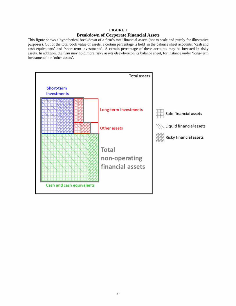
FIGURE 1 Breakdown of Corporate Financial Assets

This figure shows a hypothetical breakdown of a firm’s total financial assets (not to scale and purely for illustrative purposes). Out of the total book value of assets, a certain percentage is held in the balance sheet accounts: ‘cash and cash equivalents’ and ‘short-term investments’. A certain percentage of these accounts may be invested in risky assets. In addition, the firm may hold more risky assets elsewhere on its balance sheet, for instance under ‘long-term investments’ or ‘other assets’.

 

37

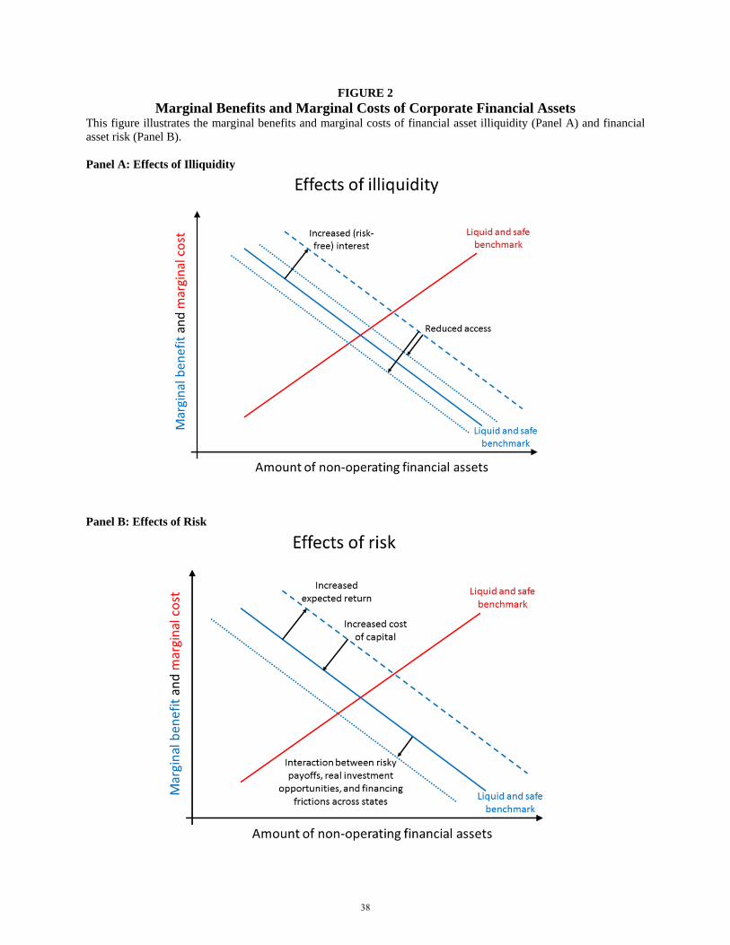
FIGURE 2 Marginal Benefits and Marginal Costs of Corporate Financial Assets

This figure illustrates the marginal benefits and marginal costs of financial asset illiquidity (Panel A) and financial asset risk (Panel B). Panel A: Effects of Illiquidity

 

Panel B: Effects of Risk

38

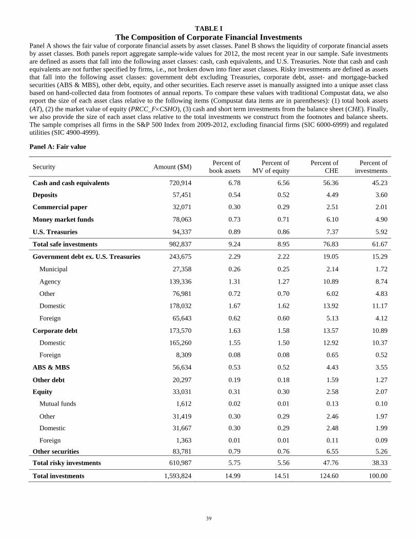
TABLE I The Composition of Corporate Financial Investments

Panel A shows the fair value of corporate financial assets by asset classes. Panel B shows the liquidity of corporate financial assets by asset classes. Both panels report aggregate sample-wide values for 2012, the most recent year in our sample. Safe investments are defined as assets that fall into the following asset classes: cash, cash equivalents, and U.S. Treasuries. Note that cash and cash equivalents are not further specified by firms, i.e., not broken down into finer asset classes. Risky investments are defined as assets that fall into the following asset classes: government debt excluding Treasuries, corporate debt, asset- and mortgage-backed securities (ABS & MBS), other debt, equity, and other securities. Each reserve asset is manually assigned into a unique asset class based on hand-collected data from footnotes of annual reports. To compare these values with traditional Compustat data, we also report the size of each asset class relative to the following items (Compustat data items are in parentheses): (1) total book assets (AT), (2) the market value of equity (PRCC_FCSHO), (3) cash and short term investments from the balance sheet (CHE). Finally, we also provide the size of each asset class relative to the total investments we construct from the footnotes and balance sheets. The sample comprises all firms in the S&P 500 Index from 2009-2012, excluding financial firms (SIC 6000-6999) and regulated utilities (SIC 4900-4999).

Panel A: Fair value

Security Amount ($M) Percent of

book assets Percent of

MV of equity Percent of

CHE Percent of

investments

Cash and cash equivalents 720,914 6.78 6.56 56.36 45.23

Deposits 57,451 0.54 0.52 4.49 3.60

Commercial paper 32,071 0.30 0.29 2.51 2.01

Money market funds 78,063 0.73 0.71 6.10 4.90

U.S. Treasuries 94,337 0.89 0.86 7.37 5.92

Total safe investments 982,837 9.24 8.95 76.83 61.67

Government debt ex. U.S. Treasuries 243,675 2.29 2.22 19.05 15.29

Municipal 27,358 0.26 0.25 2.14 1.72

Agency 139,336 1.31 1.27 10.89 8.74

Other 76,981 0.72 0.70 6.02 4.83

Domestic 178,032 1.67 1.62 13.92 11.17

Foreign 65,643 0.62 0.60 5.13 4.12

Corporate debt 173,570 1.63 1.58 13.57 10.89

Domestic 165,260 1.55 1.50 12.92 10.37

Foreign 8,309 0.08 0.08 0.65 0.52

ABS & MBS 56,634 0.53 0.52 4.43 3.55

Other debt 20,297 0.19 0.18 1.59 1.27

Equity 33,031 0.31 0.30 2.58 2.07

Mutual funds 1,612 0.02 0.01 0.13 0.10

Other 31,419 0.30 0.29 2.46 1.97

Domestic 31,667 0.30 0.29 2.48 1.99

Foreign 1,363 0.01 0.01 0.11 0.09

Other securities 83,781 0.79 0.76 6.55 5.26

Total risky investments 610,987 5.75 5.56 47.76 38.33

Total investments 1,593,824 14.99 14.51 124.60 100.00

39

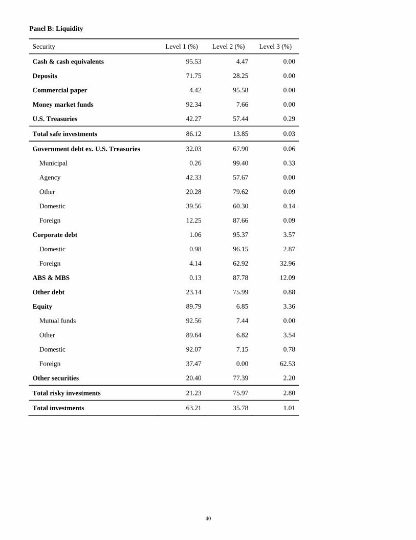
Panel B: Liquidity

Security Level 1 (%) Level 2 (%) Level 3 (%)

Cash & cash equivalents 95.53 4.47 0.00

Deposits 71.75 28.25 0.00

Commercial paper 4.42 95.58 0.00

Money market funds 92.34 7.66 0.00

U.S. Treasuries 42.27 57.44 0.29

Total safe investments 86.12 13.85 0.03

Government debt ex. U.S. Treasuries 32.03 67.90 0.06

Municipal 0.26 99.40 0.33

Agency 42.33 57.67 0.00

Other 20.28 79.62 0.09

Domestic 39.56 60.30 0.14

Foreign 12.25 87.66 0.09

Corporate debt 1.06 95.37 3.57

Domestic 0.98 96.15 2.87

Foreign 4.14 62.92 32.96

ABS & MBS 0.13 87.78 12.09

Other debt 23.14 75.99 0.88

Equity 89.79 6.85 3.36

Mutual funds 92.56 7.44 0.00

Other 89.64 6.82 3.54

Domestic 92.07 7.15 0.78

Foreign 37.47 0.00 62.53

Other securities 20.40 77.39 2.20

Total risky investments 21.23 75.97 2.80

Total investments 63.21 35.78 1.01

40

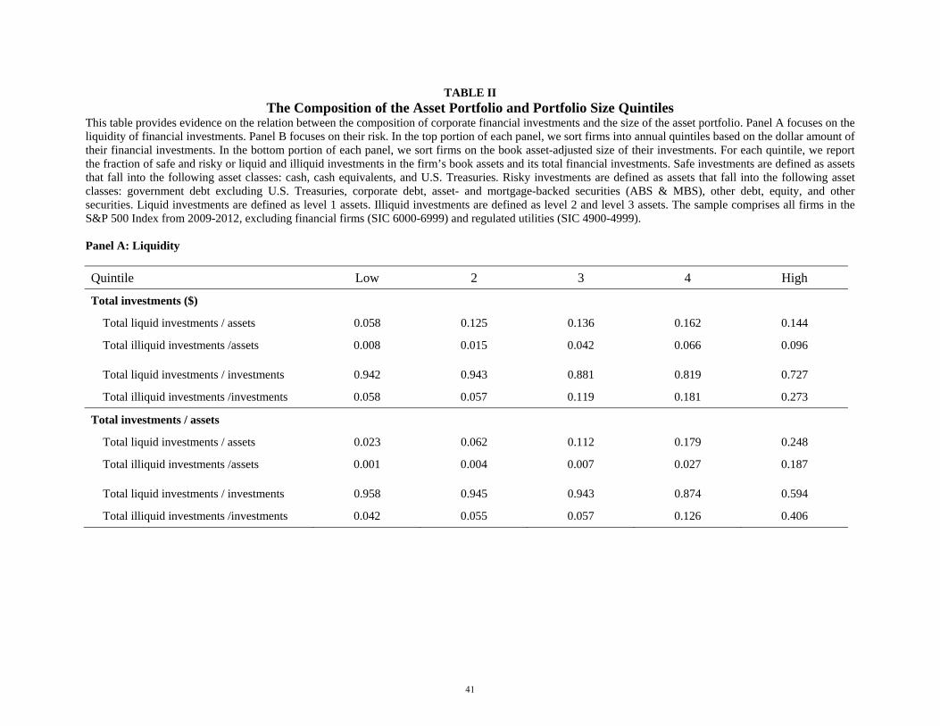
TABLE II The Composition of the Asset Portfolio and Portfolio Size Quintiles

This table provides evidence on the relation between the composition of corporate financial investments and the size of the asset portfolio. Panel A focuses on the liquidity of financial investments. Panel B focuses on their risk. In the top portion of each panel, we sort firms into annual quintiles based on the dollar amount of their financial investments. In the bottom portion of each panel, we sort firms on the book asset-adjusted size of their investments. For each quintile, we report the fraction of safe and risky or liquid and illiquid investments in the firm’s book assets and its total financial investments. Safe investments are defined as assets that fall into the following asset classes: cash, cash equivalents, and U.S. Treasuries. Risky investments are defined as assets that fall into the following asset classes: government debt excluding U.S. Treasuries, corporate debt, asset- and mortgage-backed securities (ABS & MBS), other debt, equity, and other securities. Liquid investments are defined as level 1 assets. Illiquid investments are defined as level 2 and level 3 assets. The sample comprises all firms in the S&P 500 Index from 2009-2012, excluding financial firms (SIC 6000-6999) and regulated utilities (SIC 4900-4999). Panel A: Liquidity

Quintile Low 2 3 4 High

Total investments ($)

Total liquid investments / assets 0.058 0.125 0.136 0.162 0.144

Total illiquid investments /assets 0.008 0.015 0.042 0.066 0.096

Total liquid investments / investments 0.942 0.943 0.881 0.819 0.727

Total illiquid investments /investments 0.058 0.057 0.119 0.181 0.273

Total investments / assets

Total liquid investments / assets 0.023 0.062 0.112 0.179 0.248

Total illiquid investments /assets 0.001 0.004 0.007 0.027 0.187

Total liquid investments / investments 0.958 0.945 0.943 0.874 0.594

Total illiquid investments /investments 0.042 0.055 0.057 0.126 0.406

41

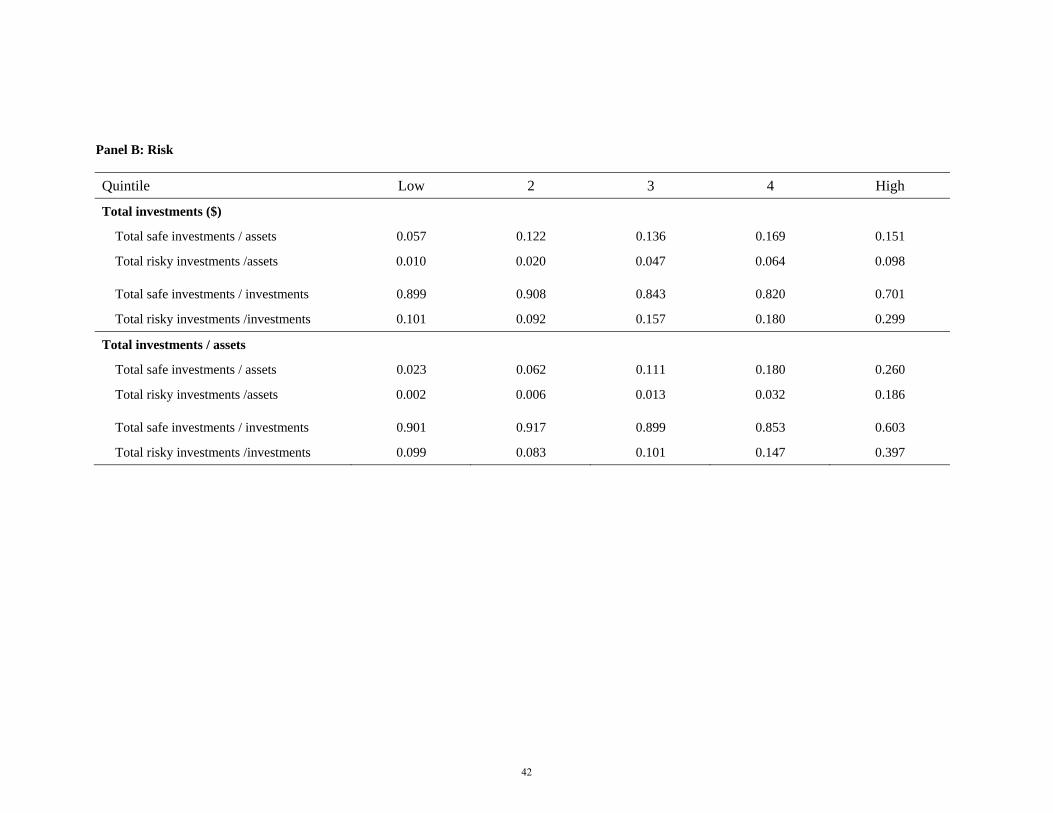
Panel B: Risk

Quintile Low 2 3 4 High

Total investments ($)

Total safe investments / assets 0.057 0.122 0.136 0.169 0.151

Total risky investments /assets 0.010 0.020 0.047 0.064 0.098

Total safe investments / investments 0.899 0.908 0.843 0.820 0.701

Total risky investments /investments 0.101 0.092 0.157 0.180 0.299

Total investments / assets

Total safe investments / assets 0.023 0.062 0.111 0.180 0.260

Total risky investments /assets 0.002 0.006 0.013 0.032 0.186

Total safe investments / investments 0.901 0.917 0.899 0.853 0.603

Total risky investments /investments 0.099 0.083 0.101 0.147 0.397

42

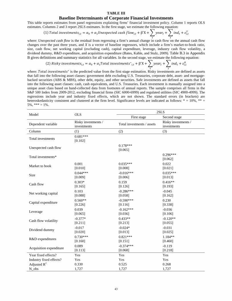
TABLE III Baseline Determinants of Corporate Financial Investments

This table reports estimates from panel regressions explaining firms’ financial investment policy. Column 1 reports OLS estimates. Columns 2 and 3 report 2SLS estimates. In the first stage, we estimate the following equation:

1 , , β X ,

where: Unexpected cash flow is the residual from regressing a firm’s annual change in cash flow on the annual cash flow changes over the past three years, and X is a vector of baseline regressors, which include a firm’s market-to-book ratio, size, cash flow, net working capital (excluding cash), capital expenditure, leverage, industry cash flow volatility, a dividend dummy, R&D expenditure, and acquisition expenditure (Bates, Kahle, and Stulz, 2009). Table B.3 in Appendix B gives definitions and summary statistics for all variables. In the second stage, we estimate the following equation:

2 , ∗, β X ,

where: ∗ is the predicted value from the first stage estimation. Risky investments are defined as assets that fall into the following asset classes: government debt excluding U.S. Treasuries, corporate debt, asset- and mortgage-backed securities (ABS & MBS), other debt, equity, and other securities. Safe investments are defined as assets that fall into the following asset classes: cash, cash equivalents, and U.S. Treasuries. Each investment is manually assigned into a unique asset class based on hand-collected data from footnotes of annual reports. The sample comprises all firms in the S&P 500 Index from 2009-2012, excluding financial firms (SIC 6000-6999) and regulated utilities (SIC 4900-4999). The regressions include year and industry fixed effects, which are not shown. The standard errors (in brackets) are heteroskedasticity consistent and clustered at the firm level. Significance levels are indicated as follows: * = 10%, ** = 5%, *** = 1%.

Model OLS 2SLS

First stage Second stage

Dependent variable Risky investments / investments

Total investments / assets Risky investments / investments

Column (1) (2) (3)

Total investments 0.681*** [0.102]

Unexpected cash flow 0.178*** [0.065]

Total investments* 0.296***

[0.062]

Market to book 0.001 0.035*** 0.022 [0.010] [0.008] [0.021]

Size 0.044*** -0.016*** 0.035*** [0.009] [0.006] [0.013]

Cash flow 0.303* 0.159 0.416** [0.165] [0.126] [0.193]

Net working capital 0.103 -0.286*** -0.045 [0.088] [0.058] [0.162]

Capital expenditure 0.560** -0.590*** 0.230 [0.226] [0.116] [0.338]

Leverage 0.039 -0.162*** -0.036 [0.065] [0.036] [0.106]

Cash flow volatility -0.377* 0.433** -0.120** [0.211] [0.213] [0.055]

Dividend dummy -0.017 -0.024* -0.031 [0.020] [0.013] [0.025]

R&D expenditures 0.730*** 0.821*** 1.184** [0.160] [0.151] [0.460]

Acquisition expenditure 0.089 -0.374*** -0.119 [0.113] [0.068] [0.218]

Year fixed effects? Yes Yes Yes Industry fixed effects? Yes Yes Yes Adjusted R2 0.330 0.525 0.268 N_obs 1,727 1,727 1,727

43

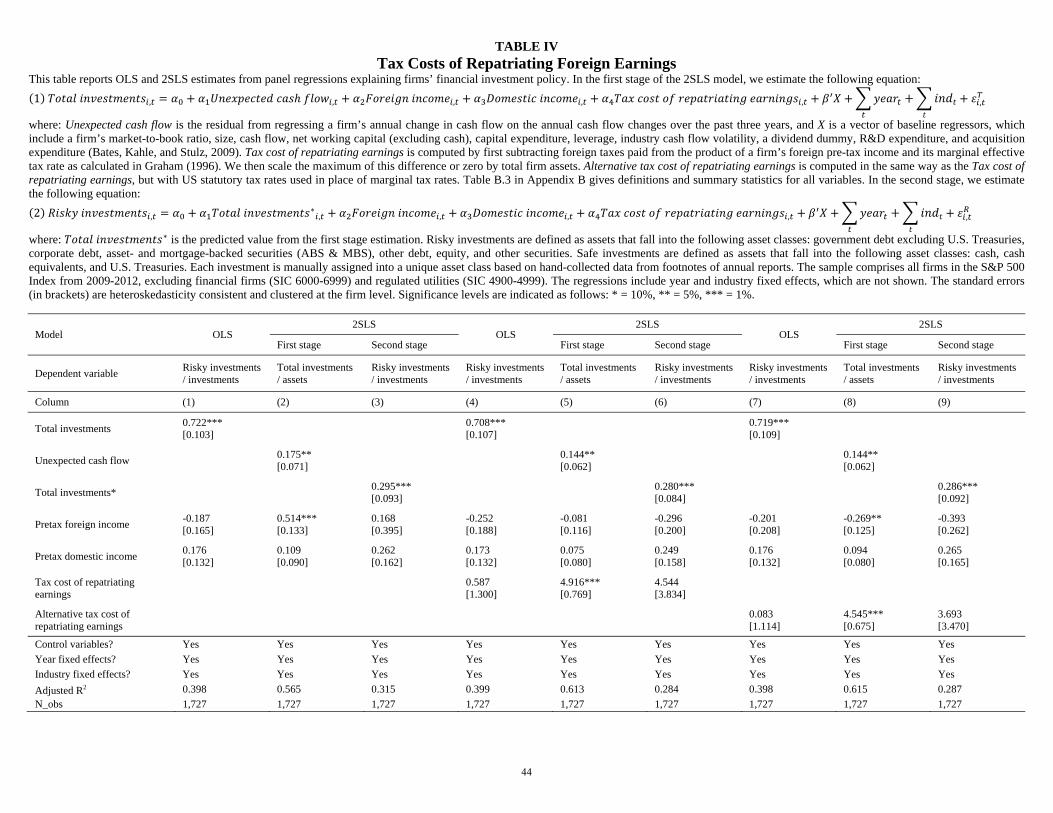
TABLE IV Tax Costs of Repatriating Foreign Earnings

This table reports OLS and 2SLS estimates from panel regressions explaining firms’ financial investment policy. In the first stage of the 2SLS model, we estimate the following equation:

1 , , , , , ,

where: Unexpected cash flow is the residual from regressing a firm’s annual change in cash flow on the annual cash flow changes over the past three years, and X is a vector of baseline regressors, which include a firm’s market-to-book ratio, size, cash flow, net working capital (excluding cash), capital expenditure, leverage, industry cash flow volatility, a dividend dummy, R&D expenditure, and acquisition expenditure (Bates, Kahle, and Stulz, 2009). Tax cost of repatriating earnings is computed by first subtracting foreign taxes paid from the product of a firm’s foreign pre-tax income and its marginal effective tax rate as calculated in Graham (1996). We then scale the maximum of this difference or zero by total firm assets. Alternative tax cost of repatriating earnings is computed in the same way as the Tax cost of repatriating earnings, but with US statutory tax rates used in place of marginal tax rates. Table B.3 in Appendix B gives definitions and summary statistics for all variables. In the second stage, we estimate the following equation:

2 , ∗, , , , ,

where: ∗ is the predicted value from the first stage estimation. Risky investments are defined as assets that fall into the following asset classes: government debt excluding U.S. Treasuries, corporate debt, asset- and mortgage-backed securities (ABS & MBS), other debt, equity, and other securities. Safe investments are defined as assets that fall into the following asset classes: cash, cash equivalents, and U.S. Treasuries. Each investment is manually assigned into a unique asset class based on hand-collected data from footnotes of annual reports. The sample comprises all firms in the S&P 500 Index from 2009-2012, excluding financial firms (SIC 6000-6999) and regulated utilities (SIC 4900-4999). The regressions include year and industry fixed effects, which are not shown. The standard errors (in brackets) are heteroskedasticity consistent and clustered at the firm level. Significance levels are indicated as follows: * = 10%, ** = 5%, *** = 1%.

Model OLS 2SLS

OLS 2SLS

OLS 2SLS

First stage Second stage First stage Second stage First stage Second stage

Dependent variable Risky investments / investments

Total investments / assets

Risky investments / investments

Risky investments / investments

Total investments / assets

Risky investments / investments

Risky investments / investments

Total investments / assets

Risky investments / investments

Column (1) (2) (3) (4) (5) (6) (7) (8) (9)

Total investments 0.722*** 0.708*** 0.719*** [0.103] [0.107] [0.109]

Unexpected cash flow 0.175** 0.144** 0.144**

[0.071] [0.062] [0.062]

Total investments* 0.295*** 0.280*** 0.286***

[0.093] [0.084] [0.092]

Pretax foreign income -0.187 0.514*** 0.168 -0.252 -0.081 -0.296 -0.201 -0.269** -0.393 [0.165] [0.133] [0.395] [0.188] [0.116] [0.200] [0.208] [0.125] [0.262]

Pretax domestic income 0.176 0.109 0.262 0.173 0.075 0.249 0.176 0.094 0.265 [0.132] [0.090] [0.162] [0.132] [0.080] [0.158] [0.132] [0.080] [0.165]

Tax cost of repatriating earnings

0.587 4.916*** 4.544 [1.300] [0.769] [3.834]

Alternative tax cost of repatriating earnings

0.083 4.545*** 3.693 [1.114] [0.675] [3.470]

Control variables? Yes Yes Yes Yes Yes Yes Yes Yes Yes

Year fixed effects? Yes Yes Yes Yes Yes Yes Yes Yes Yes

Industry fixed effects? Yes Yes Yes Yes Yes Yes Yes Yes Yes

Adjusted R2 0.398 0.565 0.315 0.399 0.613 0.284 0.398 0.615 0.287

N_obs 1,727 1,727 1,727 1,727 1,727 1,727 1,727 1,727 1,727

44

TABLE V Corporate Governance

This table reports OLS and 2SLS estimates from panel regressions explaining firms’ financial investment policy. In the first stage of the 2SLS model, we estimate the following equation:

1 , , , ,

where: Unexpected cash flow is the residual from regressing a firm’s annual change in cash flow on the annual cash flow changes over the past three years, and X is a vector of baseline regressors, which include a firm’s market-to-book ratio, size, cash flow, net working capital (excluding cash), capital expenditure, leverage, industry cash flow volatility, a dividend dummy, R&D expenditure, and acquisition expenditure (Bates, Kahle, and Stulz, 2009). G is measured using three proxies: E-Index is the Bebchuk, Cohen, and Ferrell (2009) governance index. Block holdings is the sum of all ownership positions greater than 5% held by institutional investors. Pension holdings is the sum of all ownership positions by public pension funds. Table B.3 in Appendix B gives definitions and summary statistics for all variables. In the second stage, we estimate the following equation:

2 , ∗, , ,

where: ∗ is the predicted value from the first stage estimation. Risky investments are defined as assets that fall into the following asset classes: government debt excluding U.S. Treasuries, corporate debt, asset- and mortgage-backed securities (ABS & MBS), other debt, equity, and other securities. Safe investments are defined as assets that fall into the following asset classes: cash, cash equivalents, and U.S. Treasuries. Each investment is manually assigned into a unique asset class based on hand-collected data from footnotes of annual reports. The sample comprises all firms in the S&P 500 Index from 2009-2012, excluding financial firms (SIC 6000-6999) and regulated utilities (SIC 4900-4999). The regressions include year and industry fixed effects, which are not shown. The standard errors (in brackets) are heteroskedasticity consistent and clustered at the firm level. Significance levels are indicated as follows: * = 10%, ** = 5%, *** = 1%.

Model OLS 2SLS

OLS 2SLS

OLS 2SLS

First stage Second stage First stage Second stage First stage Second stage

Dependent variable Risky investments / investments

Total investments / assets

Risky investments / investments

Risky investments / investments

Total investments / assets

Risky investments / investments

Risky investments / investments

Total investments / assets

Risky investments / investments

Column (1) (2) (3) (4) (5) (6) (7) (8) (9)

Total investments 0.713*** 0.689*** 0.656*** [0.114] [0.104] [0.112]

Unexpected cash flow 0.220*** 0.189*** 0.176**

[0.077] [0.067] [0.068]

Total investments* 0.274*** 0.291*** 0.290***

[0.082] [0.087] [0.084]

E-index 0.022* -0.013** 0.025** [0.013] [0.006] [0.011]

Block holdings -0.053*** 0.011 -0.047**

[0.019] [0.011] [0.021]

Pension holdings -0.086*** 0.004 -0.084**

[0.030] [0.021] [0.033] Control variables? Yes Yes Yes Yes Yes Yes Yes Yes Yes Year fixed effects? Yes Yes Yes Yes Yes Yes Yes Yes Yes Industry fixed effects? Yes Yes Yes Yes Yes Yes Yes Yes Yes Adjusted R2 0.334 0.554 0.326 0.337 0.522 0.264 0.313 0.508 0.255 N_obs 1,436 1,436 1,436 1,502 1,502 1,502 1,553 1,553 1,553

45

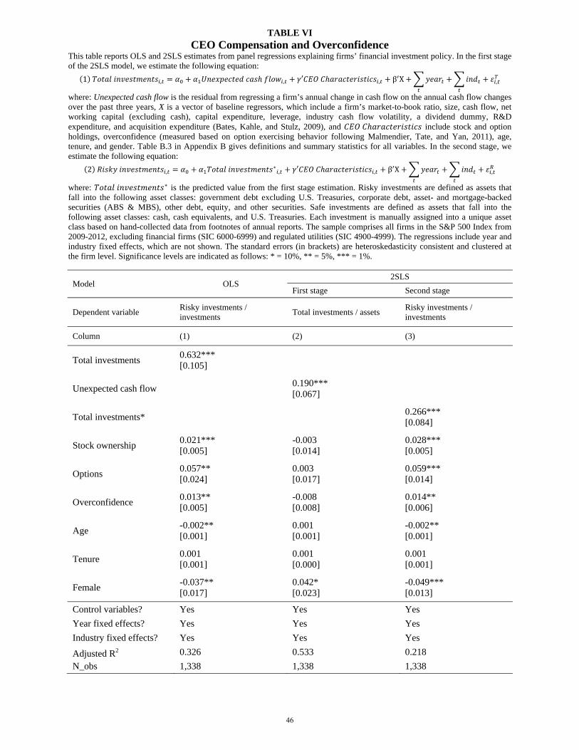
TABLE VI CEO Compensation and Overconfidence

This table reports OLS and 2SLS estimates from panel regressions explaining firms’ financial investment policy. In the first stage of the 2SLS model, we estimate the following equation:

1 , , ′ , β X ,

where: Unexpected cash flow is the residual from regressing a firm’s annual change in cash flow on the annual cash flow changes over the past three years, X is a vector of baseline regressors, which include a firm’s market-to-book ratio, size, cash flow, net working capital (excluding cash), capital expenditure, leverage, industry cash flow volatility, a dividend dummy, R&D expenditure, and acquisition expenditure (Bates, Kahle, and Stulz, 2009), and include stock and option holdings, overconfidence (measured based on option exercising behavior following Malmendier, Tate, and Yan, 2011), age, tenure, and gender. Table B.3 in Appendix B gives definitions and summary statistics for all variables. In the second stage, we estimate the following equation:

2 , ∗, ′ , β X ,

where: ∗ is the predicted value from the first stage estimation. Risky investments are defined as assets that fall into the following asset classes: government debt excluding U.S. Treasuries, corporate debt, asset- and mortgage-backed securities (ABS & MBS), other debt, equity, and other securities. Safe investments are defined as assets that fall into the following asset classes: cash, cash equivalents, and U.S. Treasuries. Each investment is manually assigned into a unique asset class based on hand-collected data from footnotes of annual reports. The sample comprises all firms in the S&P 500 Index from 2009-2012, excluding financial firms (SIC 6000-6999) and regulated utilities (SIC 4900-4999). The regressions include year and industry fixed effects, which are not shown. The standard errors (in brackets) are heteroskedasticity consistent and clustered at the firm level. Significance levels are indicated as follows: * = 10%, ** = 5%, *** = 1%.

Model OLS 2SLS

First stage Second stage

Dependent variable Risky investments / investments

Total investments / assets Risky investments / investments

Column (1) (2) (3)

Total investments 0.632*** [0.105]

Unexpected cash flow 0.190***

[0.067]

Total investments* 0.266***

[0.084]

Stock ownership 0.021*** -0.003 0.028*** [0.005] [0.014] [0.005]

Options 0.057** 0.003 0.059*** [0.024] [0.017] [0.014]

Overconfidence 0.013** -0.008 0.014** [0.005] [0.008] [0.006]

Age -0.002** 0.001 -0.002** [0.001] [0.001] [0.001]

Tenure 0.001 0.001 0.001 [0.001] [0.000] [0.001]

Female -0.037** 0.042* -0.049*** [0.017] [0.023] [0.013]

Control variables? Yes Yes Yes

Year fixed effects? Yes Yes Yes

Industry fixed effects? Yes Yes Yes

Adjusted R2 0.326 0.533 0.218

N_obs 1,338 1,338 1,338

46

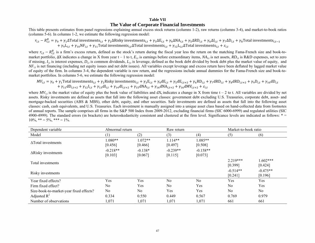
Table VII The Value of Corporate Financial Investments

This table presents estimates from panel regressions explaining annual excess stock returns (columns 1-2), raw returns (columns 3-4), and market-to-book ratios (columns 5-6). In columns 1-2, we estimate the following regression model:

, , ΔTotalinvestments , ΔRiskyinvestments , ΔE , ΔNA , ΔRD , ΔI , ΔD , Totalinvestments ,L , NF , Totalinvestments , ΔTotalinvestments , L , ΔTotalinvestments , ,

where , , is a firm’s excess return, defined as the stock’s return during the fiscal year less the return on the matching Fama-French size and book-to-market portfolio, ΔX indicates a change in X from year t – 1 to t, Ei,t is earnings before extraordinary items, NAi,t is net assets, RDi,t is R&D expenses, set to zero if missing, Ii,t is interest expenses, Di,t is common dividends, Li,t is leverage, defined as the book debt divided by book debt plus the market value of equity, and NFi,t is net financing (including net equity issues and net debt issues). All variables except leverage and excess return have been deflated by lagged market value of equity of the firm. In columns 3-4, the dependent variable is raw return, and the regressions include annual dummies for the Fama-French size and book-to-market portfolios. In columns 5-6, we estimate the following regression model:

, Totalinvestments , Riskyinvestments , E , dE , dE , RD , dRD , dRD , D , dD ,

dD , I , dI , dI , dNA , dNA , dMV , ,

where MVi,t is the market value of equity plus the book value of liabilities and dXt indicates a change in X from time t – 2 to t. All variables are divided by net assets. Risky investments are defined as assets that fall into the following asset classes: government debt excluding U.S. Treasuries, corporate debt, asset- and mortgage-backed securities (ABS & MBS), other debt, equity, and other securities. Safe investments are defined as assets that fall into the following asset classes: cash, cash equivalents, and U.S. Treasuries. Each investment is manually assigned into a unique asset class based on hand-collected data from footnotes of annual reports. The sample comprises all firms in the S&P 500 Index from 2009-2012, excluding financial firms (SIC 6000-6999) and regulated utilities (SIC 4900-4999). The standard errors (in brackets) are heteroskedasticity consistent and clustered at the firm level. Significance levels are indicated as follows: * = 10%, ** = 5%, *** = 1%. Dependent variable Abnormal return Raw return Market-to-book ratio Model (1) (2) (3) (4) (5) (6)

ΔTotal investments 1.080** 1.072** 1.114** 1.085** [0.456] [0.466] [0.497] [0.508]

ΔRisky investments -0.218** -0.138* -0.239** -0.158** [0.103] [0.067] [0.115] [0.073]

Total investments 2.219*** 1.602***

[0.399] [0.424]

Risky investments -0.514** -0.475**

[0.241] [0.196] Year fixed effects? Yes Yes No No Yes Yes Firm fixed effect? No Yes No Yes No Yes Size-book-to-market-year fixed effects? No No Yes Yes No No Adjusted R2 0.334 0.550 0.449 0.567 0.769 0.979 Number of observations 1,071 1,071 1,071 1,071 661 661

47

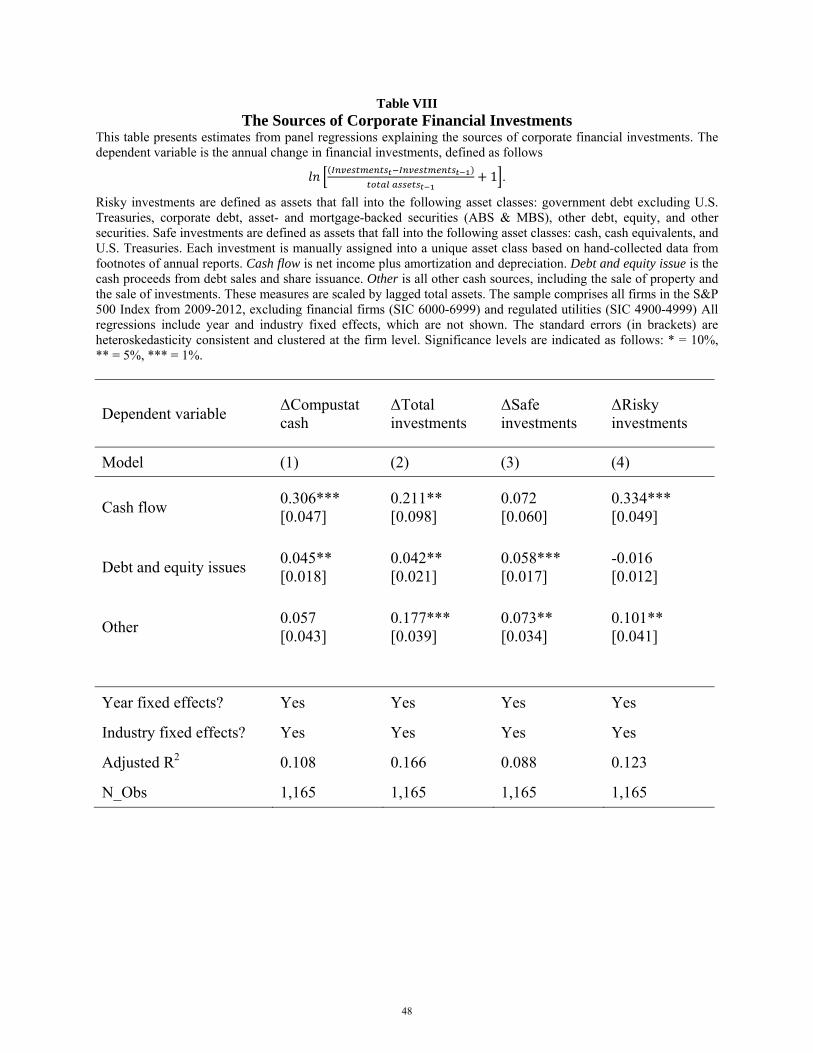
Table VIII The Sources of Corporate Financial Investments

This table presents estimates from panel regressions explaining the sources of corporate financial investments. The dependent variable is the annual change in financial investments, defined as follows

1 .

Risky investments are defined as assets that fall into the following asset classes: government debt excluding U.S. Treasuries, corporate debt, asset- and mortgage-backed securities (ABS & MBS), other debt, equity, and other securities. Safe investments are defined as assets that fall into the following asset classes: cash, cash equivalents, and U.S. Treasuries. Each investment is manually assigned into a unique asset class based on hand-collected data from footnotes of annual reports. Cash flow is net income plus amortization and depreciation. Debt and equity issue is the cash proceeds from debt sales and share issuance. Other is all other cash sources, including the sale of property and the sale of investments. These measures are scaled by lagged total assets. The sample comprises all firms in the S&P 500 Index from 2009-2012, excluding financial firms (SIC 6000-6999) and regulated utilities (SIC 4900-4999) All regressions include year and industry fixed effects, which are not shown. The standard errors (in brackets) are heteroskedasticity consistent and clustered at the firm level. Significance levels are indicated as follows: * = 10%, ** = 5%, *** = 1%.

Dependent variable ΔCompustat cash

ΔTotal investments

ΔSafe investments

ΔRisky investments

Model (1) (2) (3) (4)

Cash flow 0.306*** 0.211** 0.072 0.334*** [0.047] [0.098] [0.060] [0.049]

Debt and equity issues 0.045** 0.042** 0.058*** -0.016 [0.018] [0.021] [0.017] [0.012]

Other 0.057 0.177*** 0.073** 0.101** [0.043] [0.039] [0.034] [0.041]

Year fixed effects? Yes Yes Yes Yes

Industry fixed effects? Yes Yes Yes Yes

Adjusted R2 0.108 0.166 0.088 0.123

N_Obs 1,165 1,165 1,165 1,165

48

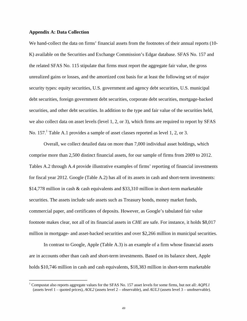
Appendix A: Data Collection

We hand-collect the data on firms’ financial assets from the footnotes of their annual reports (10-

K) available on the Securities and Exchange Commission’s Edgar database. SFAS No. 157 and

the related SFAS No. 115 stipulate that firms must report the aggregate fair value, the gross

unrealized gains or losses, and the amortized cost basis for at least the following set of major

security types: equity securities, U.S. government and agency debt securities, U.S. municipal

debt securities, foreign government debt securities, corporate debt securities, mortgage-backed

securities, and other debt securities. In addition to the type and fair value of the securities held,

we also collect data on asset levels (level 1, 2, or 3), which firms are required to report by SFAS

No. 157.1 Table A.1 provides a sample of asset classes reported as level 1, 2, or 3.

Overall, we collect detailed data on more than 7,000 individual asset holdings, which

comprise more than 2,500 distinct financial assets, for our sample of firms from 2009 to 2012.

Tables A.2 through A.4 provide illustrative examples of firms’ reporting of financial investments

for fiscal year 2012. Google (Table A.2) has all of its assets in cash and short-term investments:

$14,778 million in cash & cash equivalents and $33,310 million in short-term marketable

securities. The assets include safe assets such as Treasury bonds, money market funds,

commercial paper, and certificates of deposits. However, as Google’s tabulated fair value

footnote makes clear, not all of its financial assets in CHE are safe. For instance, it holds $8,017

million in mortgage- and asset-backed securities and over $2,266 million in municipal securities.

In contrast to Google, Apple (Table A.3) is an example of a firm whose financial assets

are in accounts other than cash and short-term investments. Based on its balance sheet, Apple

holds $10,746 million in cash and cash equivalents, $18,383 million in short-term marketable

                                                            1 Compustat also reports aggregate values for the SFAS No. 157 asset levels for some firms, but not all: AQPL1

(assets level 1 – quoted prices), AOL2 (assets level 2 – observable), and AUL3 (assets level 3 – unobservable).

49

securities, and $92,122 million in long-term marketable securities. The total fair value of their

financial instruments therefore is $121,251 million, which is the number frequently quoted in the

financial media. The tabulated fair value footnote provides a breakdown of all $121,251 million

into asset classes. For instance, $3,109 million is reported as cash, $2,462 million is reported as

level 1 mutual funds, and $20,108 million is reported as level 2 U.S. Treasury securities.

Not all reports are as transparent and easy to understand as those of Google and Apple.

Table A.4 shows that, in the case of Intel, not all their financial assets are reported in the fair

value footnotes. Indeed, their cash & cash equivalent assets do not sum up to the amount on the

balance sheet, since actual cash is missing from the footnote. Reconciling these data with the

balance sheet information is necessary in order to map out all of the firm’s financial assets.

Table A.1: Asset Classification into Levels 1, 2, or 3 The table shows a sample of the assets found in the footnotes of annual reports, which following the guidelines in SFAS No. 157, are classified into level 1, 2, or 3 depending on the input(s) required to determine their fair value.

Level 1 Level 2 Level 3 Cash Cash equivalents Mutual funds U.S. Treasury securities Equity securities Corporate bonds – non U.S. Available-for-sale securities Bank deposits Money market funds

U.S. Treasury Securities Commercial paper Corporate bonds Time deposits Corporate bonds – non U.S. Asset-backed securities Available-for-sale securities U.S. Agency securities Government bonds – non U.S. Municipal bonds and notes Other securities

Venture capital investments Corporate bonds – non U.S. Available-for-sale securities Closed-end municipal bond funds Mortgage-backed securities Auction rate securities Long-term Venezuelan bonds Convertible debt securities

50

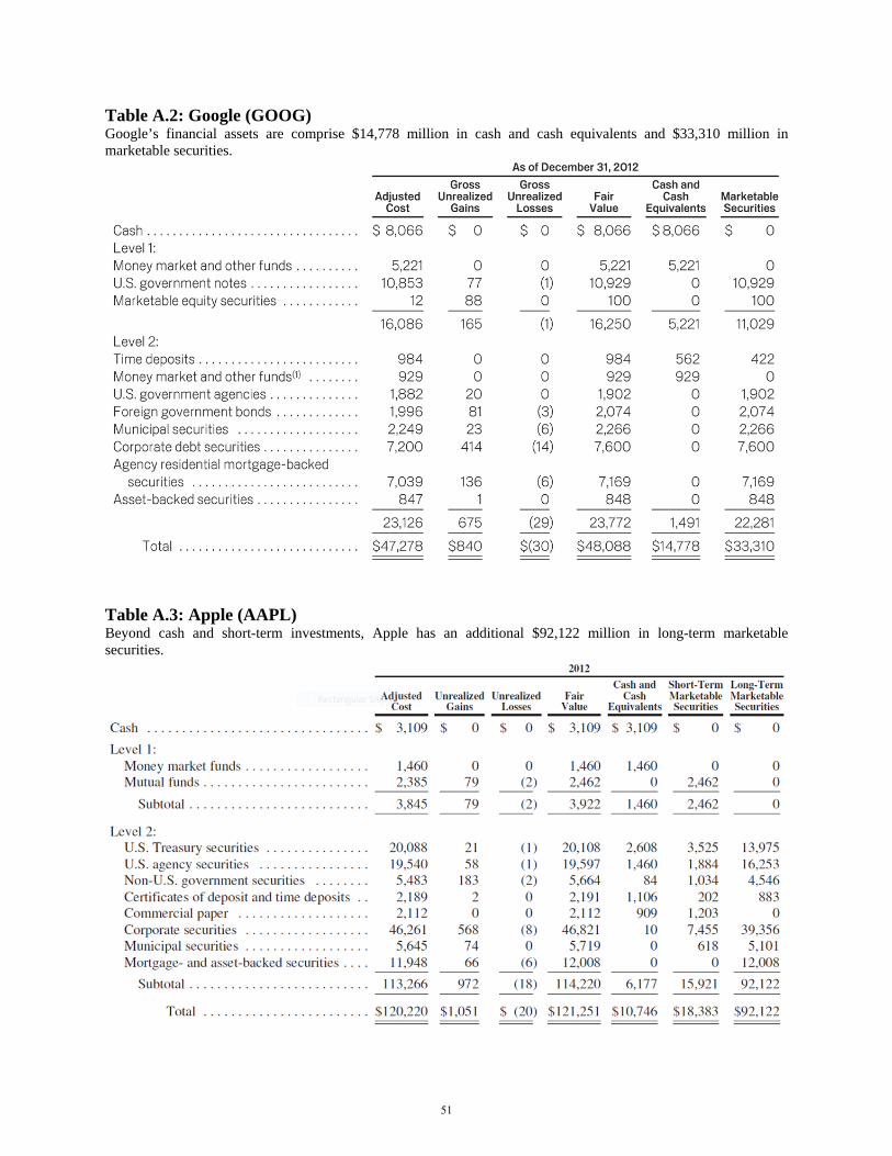
Table A.2: Google (GOOG) Google’s financial assets are comprise $14,778 million in cash and cash equivalents and $33,310 million in marketable securities.

Table A.3: Apple (AAPL) Beyond cash and short-term investments, Apple has an additional $92,122 million in long-term marketable securities.

 

51

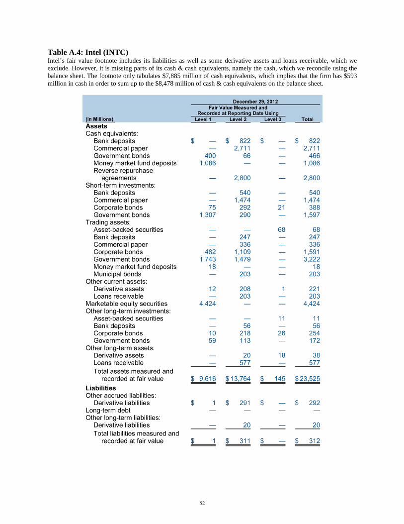
Table A.4: Intel (INTC) Intel’s fair value footnote includes its liabilities as well as some derivative assets and loans receivable, which we exclude. However, it is missing parts of its cash & cash equivalents, namely the cash, which we reconcile using the balance sheet. The footnote only tabulates $7,885 million of cash equivalents, which implies that the firm has $593 million in cash in order to sum up to the $8,478 million of cash & cash equivalents on the balance sheet.

 

52

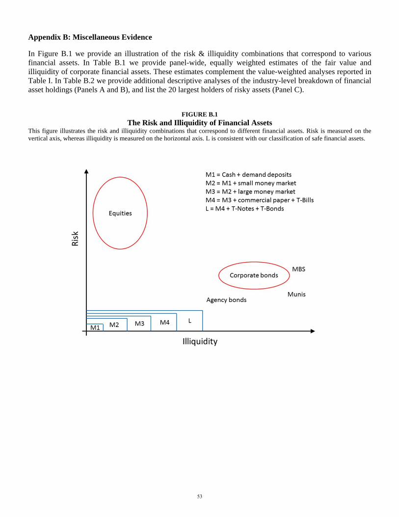
Appendix B: Miscellaneous Evidence In Figure B.1 we provide an illustration of the risk & illiquidity combinations that correspond to various financial assets. In Table B.1 we provide panel-wide, equally weighted estimates of the fair value and illiquidity of corporate financial assets. These estimates complement the value-weighted analyses reported in Table I. In Table B.2 we provide additional descriptive analyses of the industry-level breakdown of financial asset holdings (Panels A and B), and list the 20 largest holders of risky assets (Panel C).

FIGURE B.1 The Risk and Illiquidity of Financial Assets

This figure illustrates the risk and illiquidity combinations that correspond to different financial assets. Risk is measured on the vertical axis, whereas illiquidity is measured on the horizontal axis. L is consistent with our classification of safe financial assets.

53

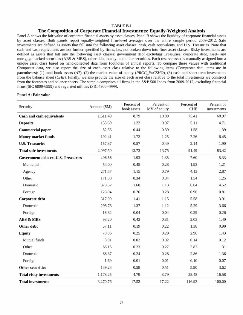
TABLE B.1 The Composition of Corporate Financial Investments: Equally-Weighted Analysis

Panel A shows the fair value of corporate financial assets by asset classes. Panel B shows the liquidity of corporate financial assets by asset classes. Both panels report equally-weighted firm-level averages over the entire sample period 2009-2012. Safe investments are defined as assets that fall into the following asset classes: cash, cash equivalents, and U.S. Treasuries. Note that cash and cash equivalents are not further specified by firms, i.e., not broken down into finer asset classes. Risky investments are defined as assets that fall into the following asset classes: government debt excluding Treasuries, corporate debt, asset- and mortgage-backed securities (ABS & MBS), other debt, equity, and other securities. Each reserve asset is manually assigned into a unique asset class based on hand-collected data from footnotes of annual reports. To compare these values with traditional Compustat data, we also report the size of each asset class relative to the following items (Compustat data items are in parentheses): (1) total book assets (AT), (2) the market value of equity (PRCC_FCSHO), (3) cash and short term investments from the balance sheet (CHE). Finally, we also provide the size of each asset class relative to the total investments we construct from the footnotes and balance sheets. The sample comprises all firms in the S&P 500 Index from 2009-2012, excluding financial firms (SIC 6000-6999) and regulated utilities (SIC 4900-4999).

Panel A: Fair value

Security Amount ($M) Percent of

book assets Percent of

MV of equity Percent of

CHE Percent of

investments

Cash and cash equivalents 1,511.49 8.79 10.80 75.41 68.97

Deposits 153.69 1.22 0.97 5.11 4.71

Commercial paper 82.55 0.44 0.39 1.58 1.39

Money market funds 192.41 1.72 1.25 7.26 6.45

U.S. Treasuries 157.37 0.57 0.49 2.14 1.90

Total safe investments 2,097.50 12.73 13.75 91.49 83.42

Government debt ex. U.S. Treasuries 496.56 1.93 1.35 7.60 5.33

Municipal 54.00 0.45 0.28 1.93 1.21

Agency 271.57 1.15 0.79 4.13 2.87

Other 171.00 0.34 0.34 1.54 1.25

Domestic 373.52 1.68 1.13 6.64 4.52

Foreign 123.04 0.26 0.28 0.96 0.81

Corporate debt 317.09 1.41 1.15 5.58 3.91

Domestic 298.78 1.37 1.12 5.29 3.66

Foreign 18.32 0.04 0.04 0.29 0.26

ABS & MBS 93.20 0.42 0.31 2.03 1.40

Other debt 57.11 0.19 0.22 1.38 0.90

Equity 70.06 0.25 0.29 2.96 1.43

Mutual funds 3.91 0.02 0.02 0.14 0.12

Other 66.15 0.23 0.27 2.82 1.31

Domestic 68.37 0.24 0.28 2.86 1.36

Foreign 1.69 0.01 0.01 0.10 0.07

Other securities 139.23 0.58 0.51 5.90 3.62

Total risky investments 1,173.25 4.79 3.79 25.45 16.58

Total investments 3,270.76 17.52 17.22 116.93 100.00

54

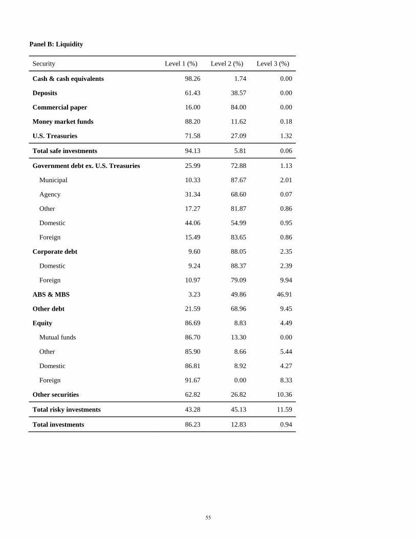
Panel B: Liquidity

Security Level 1 (%) Level 2 (%) Level 3 (%)

Cash & cash equivalents 98.26 1.74 0.00

Deposits 61.43 38.57 0.00

Commercial paper 16.00 84.00 0.00

Money market funds 88.20 11.62 0.18

U.S. Treasuries 71.58 27.09 1.32

Total safe investments 94.13 5.81 0.06

Government debt ex. U.S. Treasuries 25.99 72.88 1.13

Municipal 10.33 87.67 2.01

Agency 31.34 68.60 0.07

Other 17.27 81.87 0.86

Domestic 44.06 54.99 0.95

Foreign 15.49 83.65 0.86

Corporate debt 9.60 88.05 2.35

Domestic 9.24 88.37 2.39

Foreign 10.97 79.09 9.94

ABS & MBS 3.23 49.86 46.91

Other debt 21.59 68.96 9.45

Equity 86.69 8.83 4.49

Mutual funds 86.70 13.30 0.00

Other 85.90 8.66 5.44

Domestic 86.81 8.92 4.27

Foreign 91.67 0.00 8.33

Other securities 62.82 26.82 10.36

Total risky investments 43.28 45.13 11.59

Total investments 86.23 12.83 0.94

55

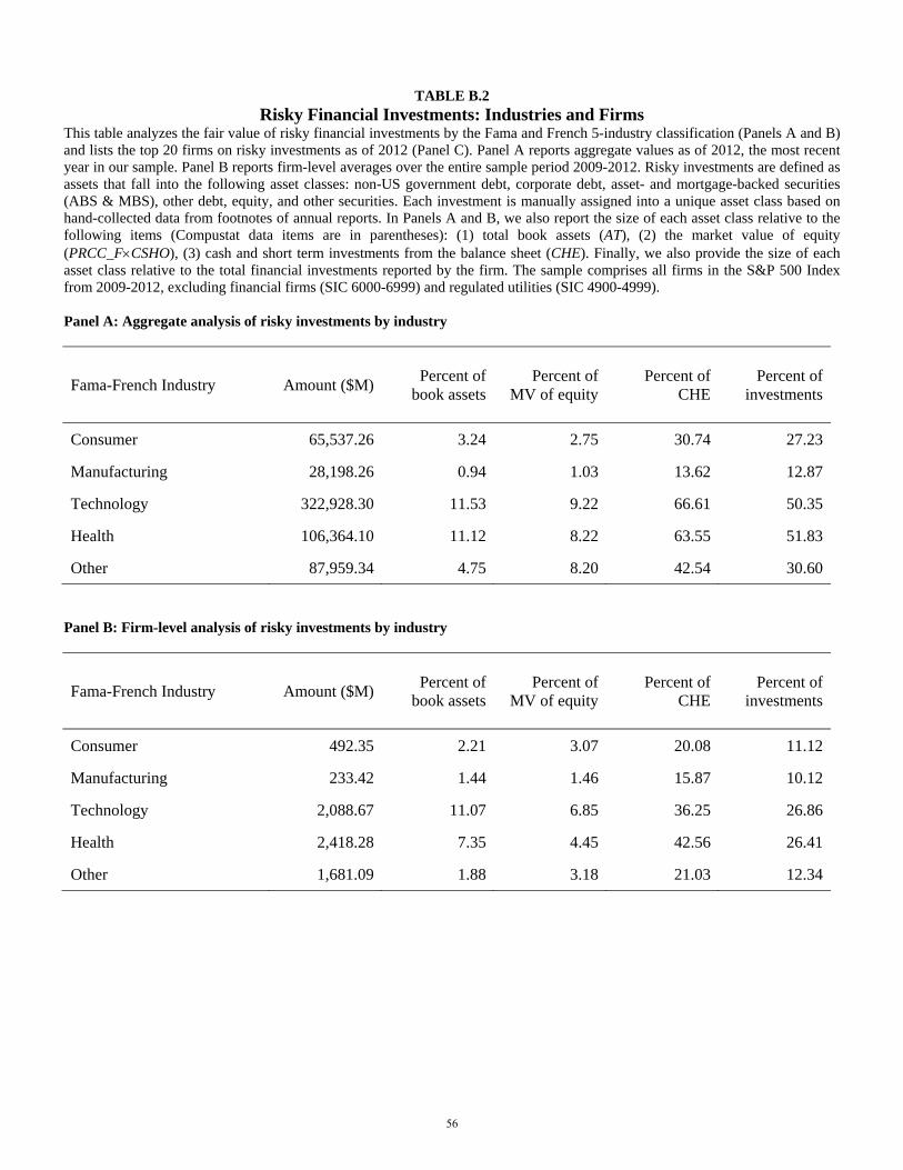
TABLE B.2 Risky Financial Investments: Industries and Firms

This table analyzes the fair value of risky financial investments by the Fama and French 5-industry classification (Panels A and B) and lists the top 20 firms on risky investments as of 2012 (Panel C). Panel A reports aggregate values as of 2012, the most recent year in our sample. Panel B reports firm-level averages over the entire sample period 2009-2012. Risky investments are defined as assets that fall into the following asset classes: non-US government debt, corporate debt, asset- and mortgage-backed securities (ABS & MBS), other debt, equity, and other securities. Each investment is manually assigned into a unique asset class based on hand-collected data from footnotes of annual reports. In Panels A and B, we also report the size of each asset class relative to the following items (Compustat data items are in parentheses): (1) total book assets (AT), (2) the market value of equity (PRCC_FCSHO), (3) cash and short term investments from the balance sheet (CHE). Finally, we also provide the size of each asset class relative to the total financial investments reported by the firm. The sample comprises all firms in the S&P 500 Index from 2009-2012, excluding financial firms (SIC 6000-6999) and regulated utilities (SIC 4900-4999). Panel A: Aggregate analysis of risky investments by industry

Fama-French Industry Amount ($M)Percent of

book assetsPercent of

MV of equityPercent of

CHE Percent of

investments

Consumer 65,537.26 3.24 2.75 30.74 27.23

Manufacturing 28,198.26 0.94 1.03 13.62 12.87

Technology 322,928.30 11.53 9.22 66.61 50.35

Health 106,364.10 11.12 8.22 63.55 51.83

Other 87,959.34 4.75 8.20 42.54 30.60

Panel B: Firm-level analysis of risky investments by industry

Fama-French Industry Amount ($M)Percent of

book assetsPercent of

MV of equityPercent of

CHE Percent of

investments

Consumer 492.35 2.21 3.07 20.08 11.12

Manufacturing 233.42 1.44 1.46 15.87 10.12

Technology 2,088.67 11.07 6.85 36.25 26.86

Health 2,418.28 7.35 4.45 42.56 26.41

Other 1,681.09 1.88 3.18 21.03 12.34

56

Panel C: Top 20 firms on risky investments in 2012

Rank Risky investments (millions of dollars) Risky investments (over total assets) Risky investments (over total investments)

Name Amount Name Percent Name Percent

1 APPLE INC 92,271 VERISIGN INC 70.58 MICROSOFT CORP 97.14

2 MICROSOFT CORP 69,480 ANALOG DEVICES 66.19 LEUCADIA NATIONAL CORP 95.83

3 GENERAL ELECTRIC CO 45,779 MICROSOFT CORP 57.29 ANALOG DEVICES 95.40

4 BERKSHIRE HATHAWAY 32,291 INTUITIVE SURGICAL INC 56.30 CF INDUSTRIES HOLDINGS INC 95.39

5 PFIZER INC 29,314 QUALCOMM INC 54.00 VERISIGN INC 93.26

6 QUALCOMM INC 23,227 XILINX INC 53.97 MEDTRONIC INC 92.38

7 GOOGLE INC 21,959 APPLE INC 52.41 TEXAS INSTRUMENTS INC 89.50

8 GENERAL MOTORS CO 18,056 F5 NETWORKS INC 51.03 WHOLE FOODS MARKET INC 87.44

9 FORD MOTOR CO 16,543 NVIDIA CORP 48.37 SANDISK CORP 86.11

10 JOHNSON & JOHNSON 15,945 SANDISK CORP 47.57 QUALCOMM INC 85.92

11 AMGEN INC 15,637 QLOGIC CORP 43.62 BIOGEN IDEC INC 84.87

12 CISCO SYSTEMS INC 14,676 LINEAR TECHNOLOGY CORP 41.27 NVIDIA CORP 83.19

13 INTEL CORP 12,396 LEUCADIA NATIONAL CORP 35.91 HELMERICH & PAYNE 83.09

14 MEDTRONIC INC 10,499 GARMIN LTD 34.06 HEALTH MANAGEMENT ASSOC 82.19

15 COCA-COLA CO 9,876 MICROCHIP TECHNOLOGY INC 33.95 F5 NETWORKS INC 81.61

16 MERCK & CO 8,052 AKAMAI TECHNOLOGIES INC 33.94 AKAMAI TECHNOLOGIES INC 80.59

17 LILLY (ELI) & CO 7,746 WATERS CORP 33.39 QLOGIC CORP 79.03

18 EMC CORP/MA 6,642 TELLABS INC 33.18 INTUITIVE SURGICAL INC 78.25

19 ORACLE CORP 4,935 KLA-TENCOR CORP 32.30 APPLIED MICRO CIRCUITS CORP 77.70

20 SANDISK CORP 4,918 NETAPP INC 32.12 LEXMARK INTL INC -CL A 77.54

57

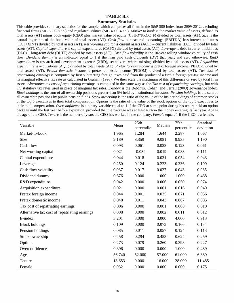
TABLE B.3 Summary Statistics

This table provides summary statistics for the sample, which comprises all firms in the S&P 500 Index from 2009-2012, excluding financial firms (SIC 6000-6999) and regulated utilities (SIC 4900-4999). Market to book is the market value of assets, defined as total assets (AT) minus book equity (CEQ) plus market value of equity (CSHO*PRCC_F) divided by total assets (AT). Size is the natural logarithm of the book value of total assets (AT). Cash flow is measured as earnings (EBITDA) less interest and taxes (TXT+XINT) divided by total assets (AT). Net working capital is current assets (ACT) – current liabilities (LCT) divided by total assets (AT). Capital expenditure is capital expenditures (CAPX) divided by total assets (AT). Leverage is debt in current liabilities (DLC) + long-term debt (DLTT) divided by total assets (AT). Cash flow volatility is the 10-year rolling window volatility of cash flow. Dividend dummy is an indicator equal to 1 if the firm paid cash dividends (DV) that year, and zero otherwise. R&D expenditure is research and development expense (XRD), set to zero where missing, divided by total assets (AT). Acquisition expenditure is acquisitions (AQC) divided by total assets (AT). Pretax foreign income is pretax foreign income (PIFO) divided by total assets (AT). Pretax domestic income is pretax domestic income (PIDOM) divided by total assets (AT). Tax cost of repatriating earnings is computed by first subtracting foreign taxes paid from the product of a firm’s foreign pre-tax income and its marginal effective tax rate as calculated in Graham (1996). We then scale the maximum of this difference or zero by total firm assets. Alternative tax cost of repatriating earnings is computed in the same way as the Tax cost of repatriating earnings, but with US statutory tax rates used in place of marginal tax rates. E-Index is the Bebchuk, Cohen, and Ferrell (2009) governance index. Block holdings is the sum of all ownership positions greater than 5% held by institutional investors. Pension holdings is the sum of all ownership positions by public pension funds. Stock ownership is the ratio of the value of the insider holdings of common stocks of the top 5 executives to their total compensation. Options is the ratio of the value of the stock options of the top 5 executives to their total compensation. Overconfidence is a binary variable equal to 1 if the CEO at some point during his tenure held an option package until the last year before expiration, provided that the package was at least 40% in the money entering its last year. Age is the age of the CEO. Tenure is the number of years the CEO has worked in the company. Female equals 1 if the CEO is a female.

Variable Mean 25th percentile

Median 75th percentile

Standard deviation

Market-to-book 1.965 1.284 1.644 2.287 1.067

Size 9.189 8.359 9.081 9.935 1.190

Cash flow 0.093 0.061 0.088 0.123 0.061

Net working capital 0.021 -0.039 0.019 0.083 0.111

Capital expenditure 0.044 0.018 0.031 0.054 0.043

Leverage 0.250 0.124 0.223 0.336 0.199

Cash flow volatility 0.037 0.017 0.027 0.043 0.035

Dividend dummy 0.676 0.000 1.000 1.000 0.468

R&D expenditure 0.042 0.000 0.006 0.050 0.074

Acquisition expenditure 0.021 0.000 0.001 0.016 0.049

Pretax foreign income 0.044 0.001 0.035 0.071 0.056

Pretax domestic income 0.048 0.011 0.043 0.087 0.085

Tax cost of repatriating earnings 0.006 0.000 0.001 0.008 0.010

Alternative tax cost of repatriating earnings 0.008 0.000 0.002 0.011 0.012

E-index 3.201 3.000 3.000 4.000 0.913

Block holdings 0.109 0.000 0.073 0.166 0.134

Pension holdings 0.085 0.011 0.057 0.124 0.113

Stock ownership 0.458 0.294 0.453 0.624 0.259

Options 0.273 0.079 0.260 0.398 0.227

Overconfidence 0.396 0.000 0.000 1.000 0.489

Age 56.740 52.000 57.000 61.000 6.389

Tenure 18.653 9.000 16.000 28.000 11.485

Female 0.032 0.000 0.000 0.000 0.175

58

 

Appendix C: Tax Effects

We first consider the case where the firm invests funds generated from domestic income (or

repatriated foreign income). Then we consider the case where the firm invests un-repatriated

foreign income. For each case, we begin by considering investments where the corporation or

individual investor can defer recognition of the taxable return for years, e.g., capital gains.

Then we consider investments that generate taxation each year on the return, e.g., dividends or

interest payments, though the investment horizon remains years.1

Domestic Reserves: Deferred Gains Taxation

Let be the corporate distribution tax rate (e.g., dividend tax rate), be the corporate earnings

tax rate, and be the individual investment earnings tax rate (e.g., capital gains rate). Consider a

financial investment, the security, with its only gain realized at a horizon of years with annual

expected gross return .

The future value of each (post-tax) dollar within the firm that is immediately distributed

to the individual investor and invested by the individual in this security is

1 1 . (C-1)

In the brackets, the first term is the gross investment return and the second term is the taxes paid

on the net return.

The future value of each dollar that the firm instead invests in the security for years

before distributing is

1 1 . (C-2)

The difference in future value between the firm investing, Equation (C-2), and the individual

investing, Equation (C-1) is

1 1 . (C-3)

If we assume that an individual facing marginal tax rate is the marginal investor, i.e.,

the discount rate that makes the present value of Equation (C-1) equal to 1 , then the

appropriate compounded risk-adjusted discount rate is

1 1 1 . (C-4)

                                                            1 For conciseness, we only consider investment gains. Investment losses may create additional tax advantages and disadvantages that are beyond the scope of this paper since such treatment would require a formal state-contingent model.

59

 

Using this discount rate, the present value of the difference between the firm investing and the

individual investing is

1 11 1 1

. (C-5)

If the corporate tax rate and individual tax rate are equal, as in the case of short-term capital

gains (both equities and fixed income), this present value is zero. Thus there is no tax advantage

or disadvantage of the firm investing in risky assets.

However, if the corporate tax rate is greater than the individual investment tax rate, such

as the case of long-term capital gains on both equities and fixed income securities, there is a loss

in present value when the firm invests rather than the individual. By taking partial derivatives we

can see that this loss is increasing in both the investment horizon and the riskiness (return) of the

investment undertaken. Investing in low return, low risk assets, i.e., the risk free asset, minimizes

this loss. The limit of this present value, Equation (C-5), as the riskiness or investment horizon

goes to infinity is

1

1. (C-6)

When the corporate tax rate is higher than the individual rate, the absolute value is the maximum

loss the firm can create by investing in risky assets. With the tax rates from the numerical

example in the main text, this maximum loss is 20% of the value that an investor would receive

from an immediate distribution.

Domestic Reserves: Intermediate (Immediate) Gains Taxation

If the taxability of investment gains cannot be delayed to the terminal period, e.g., investments in

interest bearing securities or dividend paying stocks, the present value of the difference between

the firm investing and the individual investing changes.

The future value of each dollar within the firm that is immediately distributed to the

individual investor and invested by the individual in a security with gains taxed annually and

then reinvested is

1 1 1 1 . (C-7)

Taxes thus reduce the return each year, lowering the rate of compounding.

60

 

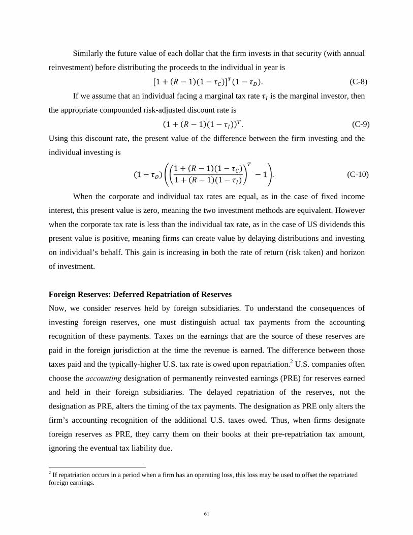
Similarly the future value of each dollar that the firm invests in that security (with annual

reinvestment) before distributing the proceeds to the individual in year is

1 1 1 1 . (C-8)

If we assume that an individual facing a marginal tax rate is the marginal investor, then

the appropriate compounded risk-adjusted discount rate is

1 1 1 . (C-9)

Using this discount rate, the present value of the difference between the firm investing and the

individual investing is

1

1 1 11 1 1

1 . (C-10)

When the corporate and individual tax rates are equal, as in the case of fixed income

interest, this present value is zero, meaning the two investment methods are equivalent. However

when the corporate tax rate is less than the individual tax rate, as in the case of US dividends this

present value is positive, meaning firms can create value by delaying distributions and investing

on individual’s behalf. This gain is increasing in both the rate of return (risk taken) and horizon

of investment.

Foreign Reserves: Deferred Repatriation of Reserves

Now, we consider reserves held by foreign subsidiaries. To understand the consequences of

investing foreign reserves, one must distinguish actual tax payments from the accounting

recognition of these payments. Taxes on the earnings that are the source of these reserves are

paid in the foreign jurisdiction at the time the revenue is earned. The difference between those

taxes paid and the typically-higher U.S. tax rate is owed upon repatriation.2 U.S. companies often

choose the accounting designation of permanently reinvested earnings (PRE) for reserves earned

and held in their foreign subsidiaries. The delayed repatriation of the reserves, not the

designation as PRE, alters the timing of the tax payments. The designation as PRE only alters the

firm’s accounting recognition of the additional U.S. taxes owed. Thus, when firms designate

foreign reserves as PRE, they carry them on their books at their pre-repatriation tax amount,

ignoring the eventual tax liability due.

                                                            2 If repatriation occurs in a period when a firm has an operating loss, this loss may be used to offset the repatriated foreign earnings.

61

 

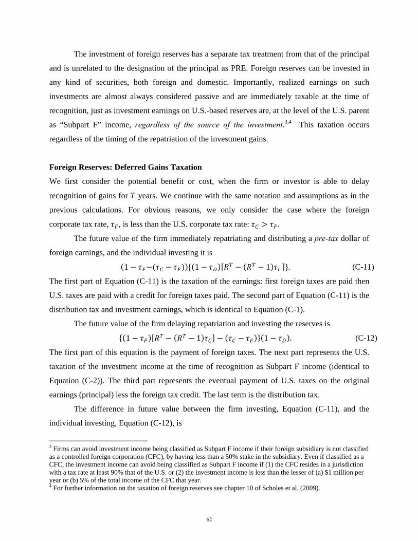
The investment of foreign reserves has a separate tax treatment from that of the principal

and is unrelated to the designation of the principal as PRE. Foreign reserves can be invested in

any kind of securities, both foreign and domestic. Importantly, realized earnings on such

investments are almost always considered passive and are immediately taxable at the time of

recognition, just as investment earnings on U.S.-based reserves are, at the level of the U.S. parent

as “Subpart F” income, regardless of the source of the investment.3,4 This taxation occurs

regardless of the timing of the repatriation of the investment gains.

Foreign Reserves: Deferred Gains Taxation

We first consider the potential benefit or cost, when the firm or investor is able to delay

recognition of gains for years. We continue with the same notation and assumptions as in the

previous calculations. For obvious reasons, we only consider the case where the foreign

corporate tax rate, , is less than the U.S. corporate tax rate: .

The future value of the firm immediately repatriating and distributing a pre-tax dollar of

foreign earnings, and the individual investing it is

1 1 1 . (C-11)

The first part of Equation (C-11) is the taxation of the earnings: first foreign taxes are paid then

U.S. taxes are paid with a credit for foreign taxes paid. The second part of Equation (C-11) is the

distribution tax and investment earnings, which is identical to Equation (C-1).

The future value of the firm delaying repatriation and investing the reserves is

1 1 1 . (C-12)

The first part of this equation is the payment of foreign taxes. The next part represents the U.S.

taxation of the investment income at the time of recognition as Subpart F income (identical to

Equation (C-2)). The third part represents the eventual payment of U.S. taxes on the original

earnings (principal) less the foreign tax credit. The last term is the distribution tax.

The difference in future value between the firm investing, Equation (C-11), and the

individual investing, Equation (C-12), is

                                                            3 Firms can avoid investment income being classified as Subpart F income if their foreign subsidiary is not classified as a controlled foreign corporation (CFC), by having less than a 50% stake in the subsidiary. Even if classified as a CFC, the investment income can avoid being classified as Subpart F income if (1) the CFC resides in a jurisdiction with a tax rate at least 90% that of the U.S. or (2) the investment income is less than the lesser of (a) $1 million per year or (b) 5% of the total income of the CFC that year. 4 For further information on the taxation of foreign reserves see chapter 10 of Scholes et al. (2009).

62

 

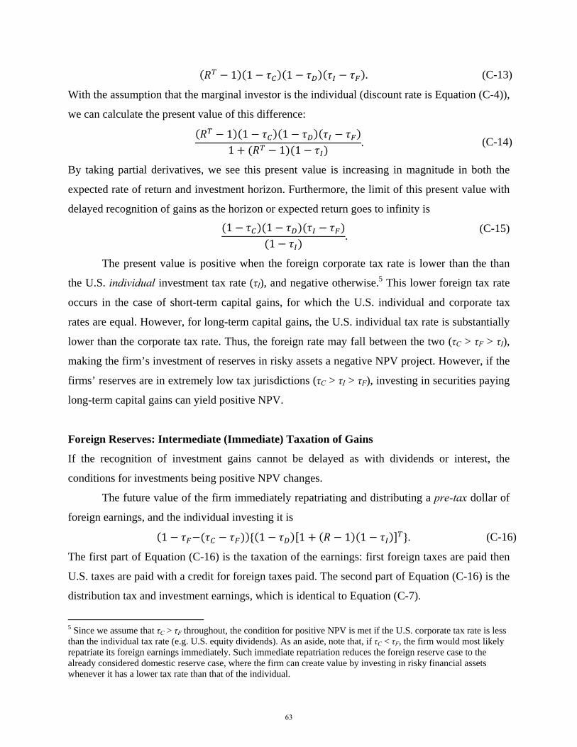
1 1 1 . (C-13)

With the assumption that the marginal investor is the individual (discount rate is Equation (C-4)),

we can calculate the present value of this difference:

1 1 11 1 1

. (C-14)

By taking partial derivatives, we see this present value is increasing in magnitude in both the

expected rate of return and investment horizon. Furthermore, the limit of this present value with

delayed recognition of gains as the horizon or expected return goes to infinity is

1 11

. (C-15)

The present value is positive when the foreign corporate tax rate is lower than the than

the U.S. individual investment tax rate (τI), and negative otherwise.5 This lower foreign tax rate

occurs in the case of short-term capital gains, for which the U.S. individual and corporate tax

rates are equal. However, for long-term capital gains, the U.S. individual tax rate is substantially

lower than the corporate tax rate. Thus, the foreign rate may fall between the two (τC > τF > τI),

making the firm’s investment of reserves in risky assets a negative NPV project. However, if the

firms’ reserves are in extremely low tax jurisdictions (τC > τI > τF), investing in securities paying

long-term capital gains can yield positive NPV.

Foreign Reserves: Intermediate (Immediate) Taxation of Gains

If the recognition of investment gains cannot be delayed as with dividends or interest, the

conditions for investments being positive NPV changes.

The future value of the firm immediately repatriating and distributing a pre-tax dollar of

foreign earnings, and the individual investing it is

1 1 1 1 1 . (C-16)

The first part of Equation (C-16) is the taxation of the earnings: first foreign taxes are paid then

U.S. taxes are paid with a credit for foreign taxes paid. The second part of Equation (C-16) is the

distribution tax and investment earnings, which is identical to Equation (C-7).

                                                            5 Since we assume that τC > τF throughout, the condition for positive NPV is met if the U.S. corporate tax rate is less than the individual tax rate (e.g. U.S. equity dividends). As an aside, note that, if τC < τF, the firm would most likely repatriate its foreign earnings immediately. Such immediate repatriation reduces the foreign reserve case to the already considered domestic reserve case, where the firm can create value by investing in risky financial assets whenever it has a lower tax rate than that of the individual.

63

 

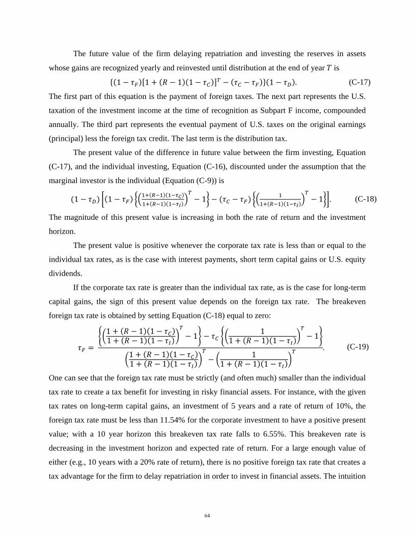
The future value of the firm delaying repatriation and investing the reserves in assets

whose gains are recognized yearly and reinvested until distribution at the end of year is

1 1 1 1 1 . (C-17)

The first part of this equation is the payment of foreign taxes. The next part represents the U.S.

taxation of the investment income at the time of recognition as Subpart F income, compounded

annually. The third part represents the eventual payment of U.S. taxes on the original earnings

(principal) less the foreign tax credit. The last term is the distribution tax.

The present value of the difference in future value between the firm investing, Equation

(C-17), and the individual investing, Equation (C-16), discounted under the assumption that the

marginal investor is the individual (Equation (C-9)) is

1 1 1 1 . (C-18)

The magnitude of this present value is increasing in both the rate of return and the investment

horizon.

The present value is positive whenever the corporate tax rate is less than or equal to the

individual tax rates, as is the case with interest payments, short term capital gains or U.S. equity

dividends.

If the corporate tax rate is greater than the individual tax rate, as is the case for long-term

capital gains, the sign of this present value depends on the foreign tax rate. The breakeven

foreign tax rate is obtained by setting Equation (C-18) equal to zero:

1 1 11 1 1 1 1

1 1 1 1

1 1 11 1 1

11 1 1

. (C-19)

One can see that the foreign tax rate must be strictly (and often much) smaller than the individual

tax rate to create a tax benefit for investing in risky financial assets. For instance, with the given

tax rates on long-term capital gains, an investment of 5 years and a rate of return of 10%, the

foreign tax rate must be less than 11.54% for the corporate investment to have a positive present

value; with a 10 year horizon this breakeven tax rate falls to 6.55%. This breakeven rate is

decreasing in the investment horizon and expected rate of return. For a large enough value of

either (e.g., 10 years with a 20% rate of return), there is no positive foreign tax rate that creates a

tax advantage for the firm to delay repatriation in order to invest in financial assets. The intuition

64

 

is that the delayed taxation of the principal from foreign reserves offsets the tax disadvantage of

the gains being taxed at the higher U.S. corporate rate.

Potential Changes Tax Code Changes

The preceding argument relied on the assumption of constant corporate tax rates. If corporations

expect tax rates to fall in the future, their incentives to invest in risky securities increase only in

some cases.

If they expect corporate tax rates to fall on all sources of earnings, then the corporations

will have increased incentives to invest in risky securities with gains whose recognition can be

deferred until after the tax decrease. However, their willingness to invest in securities that accrue

taxable gain in the interim, e.g., bonds and dividend paying stocks, will remain unchanged as

they will incur taxation on those gains at the current rate. After the tax reduction, firms may

choose to invest in riskier securities with intermediate gains.

If corporate tax rates on all earnings remain constant, but firms expect another

repatriation tax holiday, firms have no incentive to increase their investments in risky securities.

The intuition is that the repatriation tax holiday reduces the tax liability on the principal of their

investments (the unrepatriated foreign earnings), but does not reduce the tax liability on their

investment gains, which qualify as subpart F income.

65

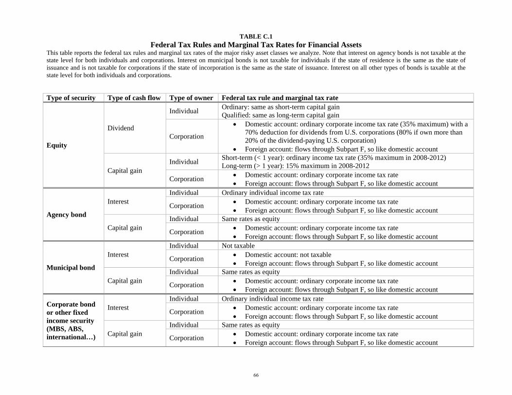
TABLE C.1 Federal Tax Rules and Marginal Tax Rates for Financial Assets

This table reports the federal tax rules and marginal tax rates of the major risky asset classes we analyze. Note that interest on agency bonds is not taxable at the state level for both individuals and corporations. Interest on municipal bonds is not taxable for individuals if the state of residence is the same as the state of issuance and is not taxable for corporations if the state of incorporation is the same as the state of issuance. Interest on all other types of bonds is taxable at the state level for both individuals and corporations.  

Type of security Type of cash flow Type of owner Federal tax rule and marginal tax rate

Equity

Dividend

Individual Ordinary: same as short-term capital gain Qualified: same as long-term capital gain

Corporation

Domestic account: ordinary corporate income tax rate (35% maximum) with a 70% deduction for dividends from U.S. corporations (80% if own more than 20% of the dividend-paying U.S. corporation)

Foreign account: flows through Subpart F, so like domestic account

Capital gain Individual

Short-term (< 1 year): ordinary income tax rate (35% maximum in 2008-2012) Long-term (> 1 year): 15% maximum in 2008-2012

Corporation Domestic account: ordinary corporate income tax rate Foreign account: flows through Subpart F, so like domestic account

Agency bond

Interest Individual Ordinary individual income tax rate

Corporation Domestic account: ordinary corporate income tax rate Foreign account: flows through Subpart F, so like domestic account

Capital gain Individual Same rates as equity

Corporation Domestic account: ordinary corporate income tax rate Foreign account: flows through Subpart F, so like domestic account

Municipal bond

Interest Individual Not taxable

Corporation Domestic account: not taxable Foreign account: flows through Subpart F, so like domestic account

Capital gain Individual Same rates as equity

Corporation Domestic account: ordinary corporate income tax rate Foreign account: flows through Subpart F, so like domestic account

Corporate bond or other fixed income security (MBS, ABS, international…)

Interest Individual Ordinary individual income tax rate

Corporation Domestic account: ordinary corporate income tax rate Foreign account: flows through Subpart F, so like domestic account

Capital gain Individual Same rates as equity

Corporation Domestic account: ordinary corporate income tax rate Foreign account: flows through Subpart F, so like domestic account

66