Preacher, K. J., & Hancock, G. R. (submitted)....
54
Online appendix to accompany: Preacher, K. J., & Hancock, G. R. (submitted). Meaningful aspects of change as novel random coefficients: A general method for reparameterizing longitudinal models. Contents 1. Mplus syntax for a reparameterized inverse quadratic function 2. Mplus syntax for an unconditional bilinear spline model 3. Mplus syntax for a conditional bilinear spline model 4. Mplus syntax for a negative exponential function with intercept, asymptote, and rate 5. Mplus syntax for a negative exponential function with intercept, rhalf-life, and ARC 6. Mathematica code for obtaining partial derivatives of an exponential function 7. Mplus syntax for a quadratic function fit to Kanfer & Ackerman's data 8. Derivation of Equation 11: Reparameterization of a bilinear spline target function 9. Annotated output: inverse quadratic function 10. Annotated output: unconditional bilinear spline model 11. Annotated output: conditional bilinear spline model 12. Annotated output: negative exponential function with intercept, asymptote, and rate 13. Annotated output: negative exponential function with intercept, half-life, and ARC 14. Annotated output: quadratic function fit to Kanfer & Ackerman’s data (traditional) 15. Annotated output: quadratic function fit to Kanfer & Ackerman’s data (modified) 1. Mplus syntax for a reparameterized inverse quadratic function The data may be obtained from Marie Davidian's website: http://www4.stat.ncsu.edu/~davidian/data/theophylline.dat The data file should be transformed to wide format prior to analysis.) TITLE: davidian theophylline data, inverse quadratic; DATA: FILE IS theophylline_wide.dat; !data file in ascii format VARIABLE: NAMES ARE subject dose wt t1-t11 conc1-conc11; !all 25 variables !subject: subject ID !dose: oral dose of theophylline in mg/kg !wt: subject weight in kg !t1-t11: time since administration of dose in hours !conc1-conc11: theophylline concentration in mg/L USEVARIABLES ARE conc1-conc11; !we plan to model 11 variables CONSTRAINT ARE t1-t11; !individual-specific time scores for use in loadings ANALYSIS: ESTIMATOR=ML; ITERATIONS=2000; CONVERGENCE=.001; !estimation options !BOOTSTRAP=5000; !for bootstrap confidence intervals if desired MODEL: [conc1-conc11*](z1-z11); !mean trend (z's defined below) conc1-conc11*.7(ve); !residual variances constrained equal conc1-conc10 PWITH conc2-conc11*.2(ve2); !optional lag-1 residual covariances b*.002(vb); c@0; m*.5(vm); !random coeff. variances (only for maximizer and theta1) b WITH c@0; b WITH m*; c WITH m@0; !random coefficient covariances [b@0 c@0 m@0]; !factor means constrained to zero b BY conc1*(b1); b BY conc2-conc11*(b2-b11); !loadings for the theta1 parameter (b) c BY conc1*(c1); c BY conc2-conc11*(c2-c11); !loadings for the theta2 parameter (c) m BY conc1*(m1); m BY conc2-conc11*(m2-m11); !loadings for the maximizer parameter (m)
-
Upload
duongkhuong -
Category
Documents
-
view
214 -
download
0
Transcript of Preacher, K. J., & Hancock, G. R. (submitted)....

Online appendix to accompany:
Preacher, K. J., & Hancock, G. R. (submitted). Meaningful aspects of change as novel random
coefficients: A general method for reparameterizing longitudinal models.
Contents
1. Mplus syntax for a reparameterized inverse quadratic function
2. Mplus syntax for an unconditional bilinear spline model
3. Mplus syntax for a conditional bilinear spline model
4. Mplus syntax for a negative exponential function with intercept, asymptote, and rate
5. Mplus syntax for a negative exponential function with intercept, rhalf-life, and ARC
6. Mathematica code for obtaining partial derivatives of an exponential function
7. Mplus syntax for a quadratic function fit to Kanfer & Ackerman's data
8. Derivation of Equation 11: Reparameterization of a bilinear spline target function
9. Annotated output: inverse quadratic function
10. Annotated output: unconditional bilinear spline model
11. Annotated output: conditional bilinear spline model
12. Annotated output: negative exponential function with intercept, asymptote, and rate
13. Annotated output: negative exponential function with intercept, half-life, and ARC
14. Annotated output: quadratic function fit to Kanfer & Ackerman’s data (traditional)
15. Annotated output: quadratic function fit to Kanfer & Ackerman’s data (modified)
1. Mplus syntax for a reparameterized inverse quadratic function
The data may be obtained from Marie Davidian's website:
http://www4.stat.ncsu.edu/~davidian/data/theophylline.dat
The data file should be transformed to wide format prior to analysis.)
TITLE: davidian theophylline data, inverse quadratic;
DATA: FILE IS theophylline_wide.dat; !data file in ascii format
VARIABLE: NAMES ARE subject dose wt t1-t11 conc1-conc11; !all 25 variables
!subject: subject ID
!dose: oral dose of theophylline in mg/kg
!wt: subject weight in kg
!t1-t11: time since administration of dose in hours
!conc1-conc11: theophylline concentration in mg/L
USEVARIABLES ARE conc1-conc11; !we plan to model 11 variables
CONSTRAINT ARE t1-t11; !individual-specific time scores for use in loadings
ANALYSIS: ESTIMATOR=ML; ITERATIONS=2000; CONVERGENCE=.001; !estimation options
!BOOTSTRAP=5000; !for bootstrap confidence intervals if desired
MODEL:
[conc1-conc11*](z1-z11); !mean trend (z's defined below)
conc1-conc11*.7(ve); !residual variances constrained equal
conc1-conc10 PWITH conc2-conc11*.2(ve2); !optional lag-1 residual covariances
b*.002(vb); c@0; m*.5(vm); !random coeff. variances (only for maximizer and theta1)
b WITH c@0; b WITH m*; c WITH m@0; !random coefficient covariances
[b@0 c@0 m@0]; !factor means constrained to zero
b BY conc1*(b1); b BY conc2-conc11*(b2-b11); !loadings for the theta1 parameter (b)
c BY conc1*(c1); c BY conc2-conc11*(c2-c11); !loadings for the theta2 parameter (c)
m BY conc1*(m1); m BY conc2-conc11*(m2-m11); !loadings for the maximizer parameter (m)

MODEL CONSTRAINT:
NEW(mb*.07 mc*.02 mm*1.77); !starts for theta1, theta2, and maximizer parameters
!intercepts constrained equal to target function
z1=t1/(mb*t1+mc*(mm^2+t1^2));
z2=t2/(mb*t2+mc*(mm^2+t2^2));
z3=t3/(mb*t3+mc*(mm^2+t3^2));
z4=t4/(mb*t4+mc*(mm^2+t4^2));
z5=t5/(mb*t5+mc*(mm^2+t5^2));
z6=t6/(mb*t6+mc*(mm^2+t6^2));
z7=t7/(mb*t7+mc*(mm^2+t7^2));
z8=t8/(mb*t8+mc*(mm^2+t8^2));
z9=t9/(mb*t9+mc*(mm^2+t9^2));
z10=t10/(mb*t10+mc*(mm^2+t10^2));
z11=t11/(mb*t11+mc*(mm^2+t11^2));
!loadings for "theta1" factor, constrained equal to d(y)/d(mb)
b1=-1*t1^2/(mb*t1+mc*(mm^2+t1^2))^2;
b2=-1*t2^2/(mb*t2+mc*(mm^2+t2^2))^2;
b3=-1*t3^2/(mb*t3+mc*(mm^2+t3^2))^2;
b4=-1*t4^2/(mb*t4+mc*(mm^2+t4^2))^2;
b5=-1*t5^2/(mb*t5+mc*(mm^2+t5^2))^2;
b6=-1*t6^2/(mb*t6+mc*(mm^2+t6^2))^2;
b7=-1*t7^2/(mb*t7+mc*(mm^2+t7^2))^2;
b8=-1*t8^2/(mb*t8+mc*(mm^2+t8^2))^2;
b9=-1*t9^2/(mb*t9+mc*(mm^2+t9^2))^2;
b10=-1*t10^2/(mb*t10+mc*(mm^2+t10^2))^2;
b11=-1*t11^2/(mb*t11+mc*(mm^2+t11^2))^2;
!loadings for "theta2" factor, constrained equal to d(y)/d(mc)
c1=-1*t1*(mm^2+t1^2)/(mb*t1+mc*(mm^2+t1^2))^2; !not strictly necessary
c2=-1*t2*(mm^2+t2^2)/(mb*t2+mc*(mm^2+t2^2))^2; !here because this
c3=-1*t3*(mm^2+t3^2)/(mb*t3+mc*(mm^2+t3^2))^2; !coefficient is fixed,
c4=-1*t4*(mm^2+t4^2)/(mb*t4+mc*(mm^2+t4^2))^2; !but included for
c5=-1*t5*(mm^2+t5^2)/(mb*t5+mc*(mm^2+t5^2))^2; !completeness.
c6=-1*t6*(mm^2+t6^2)/(mb*t6+mc*(mm^2+t6^2))^2;
c7=-1*t7*(mm^2+t7^2)/(mb*t7+mc*(mm^2+t7^2))^2;
c8=-1*t8*(mm^2+t8^2)/(mb*t8+mc*(mm^2+t8^2))^2;
c9=-1*t9*(mm^2+t9^2)/(mb*t9+mc*(mm^2+t9^2))^2;
c10=-1*t10*(mm^2+t10^2)/(mb*t10+mc*(mm^2+t10^2))^2;
c11=-1*t11*(mm^2+t11^2)/(mb*t11+mc*(mm^2+t11^2))^2;
!loadings for "maximizer" factor, constrained equal to d(y)/d(mm)
m1=-2*mm*mc*t1/(mb*t1+mc*(mm^2+t1^2))^2;
m2=-2*mm*mc*t2/(mb*t2+mc*(mm^2+t2^2))^2;
m3=-2*mm*mc*t3/(mb*t3+mc*(mm^2+t3^2))^2;
m4=-2*mm*mc*t4/(mb*t4+mc*(mm^2+t4^2))^2;
m5=-2*mm*mc*t5/(mb*t5+mc*(mm^2+t5^2))^2;
m6=-2*mm*mc*t6/(mb*t6+mc*(mm^2+t6^2))^2;
m7=-2*mm*mc*t7/(mb*t7+mc*(mm^2+t7^2))^2;
m8=-2*mm*mc*t8/(mb*t8+mc*(mm^2+t8^2))^2;
m9=-2*mm*mc*t9/(mb*t9+mc*(mm^2+t9^2))^2;
m10=-2*mm*mc*t10/(mb*t10+mc*(mm^2+t10^2))^2;
m11=-2*mm*mc*t11/(mb*t11+mc*(mm^2+t11^2))^2;
OUTPUT: TECH1; !CINTERVAL(BCBOOTSTRAP);
2. Mplus syntax for an unconditional bilinear spline model
TITLE: zerbe glucose;

DATA: FILE IS glucose.dat; !data file in ascii format
VARIABLE: NAMES ARE obese ph1-ph8; !all 9 variables
!obese: obesity status, 0=control, 1=obese
!ph1-ph8: plasma phosphate concentration repeated measures
USEVARIABLES ARE ph1-ph8; !we plan to model 8 variables
!ANALYSIS: BOOTSTRAP IS 1000; !for bootstrap confidence intervals if desired
MODEL:
[ph1-ph8*](z1-z8); !mean trend (z's defined below)
ph1-ph8*(ve); !residual variances constrained equal
w1-w4*; !random coefficient variances
w1 WITH w2*; w1 WITH w3*; w1 WITH w4*; !random coefficient covariances
w2 WITH w3*; w2 WITH w4*; w3 WITH w4*; !random coefficient covariances
[w1@0 w2@0 w3@0 w4@0]; !factor means constrained to zero
w1 BY ph1-ph8@1; !loadings for 1st factor, constrained to 1
w2 BY ph1*(w21); w2 BY ph2-ph8(w22-w28); !loadings for 2nd factor, defined below
w3 BY ph1*(w31); w3 BY ph2-ph8(w32-w38); !loadings for 3rd factor, defined below
w4 BY ph1*(w41); w4 BY ph2-ph8(w42-w48); !loadings for knot factor, defined below
MODEL CONSTRAINT:
!starts for parameters of the target function
NEW(mw1*3.4 mw2*-.26 mw3*.54 mw4*1.6 b1-b4);
!intercepts constrained equal to target function
z1=mw1+mw2*0.0+mw3*sqrt((0.0-mw4)^2);
z2=mw1+mw2*0.5+mw3*sqrt((0.5-mw4)^2);
z3=mw1+mw2*1.0+mw3*sqrt((1.0-mw4)^2);
z4=mw1+mw2*1.5+mw3*sqrt((1.5-mw4)^2);
z5=mw1+mw2*2.0+mw3*sqrt((2.0-mw4)^2);
z6=mw1+mw2*3.0+mw3*sqrt((3.0-mw4)^2);
z7=mw1+mw2*4.0+mw3*sqrt((4.0-mw4)^2);
z8=mw1+mw2*5.0+mw3*sqrt((5.0-mw4)^2);
!loadings for 2nd and 3rd factors, constrained to d(y)/d(mw2) and d(y)/d(mw3)
w21=0.0; w31=sqrt((0.0-mw4)^2);
w22=0.5; w32=sqrt((0.5-mw4)^2);
w23=1.0; w33=sqrt((1.0-mw4)^2);
w24=1.5; w34=sqrt((1.5-mw4)^2);
w25=2.0; w35=sqrt((2.0-mw4)^2);
w26=3.0; w36=sqrt((3.0-mw4)^2);
w27=4.0; w37=sqrt((4.0-mw4)^2);
w28=5.0; w38=sqrt((5.0-mw4)^2);
!loadings for knot factor, constrained to d(y)/d(mw4)
w41=(mw3*(mw4-0.0))/sqrt((0.0-mw4)^2);
w42=(mw3*(mw4-0.5))/sqrt((0.5-mw4)^2);
w43=(mw3*(mw4-1.0))/sqrt((1.0-mw4)^2);
w44=(mw3*(mw4-1.5))/sqrt((1.5-mw4)^2);
w45=(mw3*(mw4-2.0))/sqrt((2.0-mw4)^2);
w46=(mw3*(mw4-3.0))/sqrt((3.0-mw4)^2);
w47=(mw3*(mw4-4.0))/sqrt((4.0-mw4)^2);
w48=(mw3*(mw4-5.0))/sqrt((5.0-mw4)^2);
!parameters of original parameterization
b1=mw1+mw3*mw4;
b2=mw2-mw3;
b3=mw1-mw3*mw4;
b4=mw2+mw3;
OUTPUT: TECH1; !CINTERVAL(BCBOOTSTRAP);

Zerbe's (1979) data (N = 33), obtained from Zerbe (1979, p. 219).
0 3.4 3.3 3.0 2.6 2.2 2.5 3.4 4.4
0 3.7 2.6 2.6 1.9 2.9 3.2 3.1 3.9
0 4.0 4.1 3.1 2.3 2.9 3.1 3.9 4.0
0 3.6 3.0 2.2 2.8 2.9 3.9 3.8 4.0
0 4.1 3.8 2.1 3.0 3.6 3.4 3.6 3.7
0 3.8 2.2 2.0 2.6 3.8 3.6 3.0 3.5
0 3.8 3.0 2.4 2.5 3.1 3.4 3.5 3.7
0 4.4 3.9 2.8 2.1 3.6 3.8 4.0 3.9
0 5.0 4.0 3.4 3.4 3.3 3.6 4.0 4.3
0 3.7 3.1 2.9 2.2 1.5 2.3 2.7 2.8
0 3.7 2.6 2.6 2.3 2.9 2.2 3.1 3.9
0 4.4 3.7 3.1 3.2 3.7 4.3 3.9 4.8
0 4.7 3.1 3.2 3.3 3.2 4.2 3.7 4.3
1 4.3 3.3 3.0 2.6 2.2 2.5 2.4 3.4
1 5.0 4.9 4.1 3.7 3.7 4.1 4.7 4.9
1 4.6 4.4 3.9 3.9 3.7 4.2 4.8 5.0
1 4.3 3.9 3.1 3.1 3.1 3.1 3.6 4.0
1 3.1 3.1 3.3 2.6 2.6 1.9 2.3 2.7
1 4.8 5.0 2.9 2.8 2.2 3.1 3.5 3.6
1 3.7 3.1 3.3 2.8 2.9 3.6 4.3 4.4
1 5.4 4.7 3.9 4.1 2.8 3.7 3.5 3.7
1 3.0 2.5 2.3 2.2 2.1 2.6 3.2 3.5
1 4.9 5.0 4.1 3.7 3.7 4.1 4.7 4.9
1 4.8 4.3 4.7 4.6 4.7 3.7 3.6 3.9
1 4.4 4.2 4.2 3.4 3.5 3.4 3.9 4.0
1 4.9 4.3 4.0 4.0 3.3 4.1 4.2 4.3
1 5.1 4.1 4.6 4.1 3.4 4.2 4.4 4.9
1 4.8 4.6 4.6 4.4 4.1 4.0 3.8 3.8
1 4.2 3.5 3.8 3.6 3.3 3.1 3.5 3.9
1 6.6 6.1 5.2 4.1 4.3 3.8 4.2 4.8
1 3.6 3.4 3.1 2.8 2.1 2.4 2.5 3.5
1 4.5 4.0 3.7 3.3 2.4 2.3 3.1 3.3
1 4.6 4.4 3.8 3.8 3.8 3.6 3.8 3.8
3. Mplus syntax for a conditional bilinear spline model
The data may be obtained from Zerbe (1979, p. 219).
TITLE: zerbe glucose;
DATA: FILE IS glucose.dat; !data file in ascii format
DEFINE: xobese=abs(obese-1); !1=control; 0=obese
VARIABLE: NAMES ARE obese ph1-ph8; !all 9 variables
!obese: obesity status, 0=control, 1=obese
!ph1-ph8: plasma phosphate concentration repeated measures
USEVARIABLES ARE ph1-ph8 xobese; !we plan to model 9 variables
!ANALYSIS: BOOTSTRAP IS 1000; !for bootstrap confidence intervals if desired
MODEL:
[ph1-ph8*](z1-z8); !mean trend (z's defined below)
ph1-ph8*(ve); !residual variances constrained equal
w1-w4*; !random coefficient residual variances
w1 WITH w2*; w1 WITH w3*; w1 WITH w4*; !random coefficient residual covariances
w2 WITH w3*; w2 WITH w4*; w3 WITH w4*; !random coefficient residual covariances
[w1@0 w2@0 w3@0 w4@0]; !factor intercepts constrained to zero
w1 BY ph1-ph8@1; !loadings for 1st factor, constrained to 1
w2 BY ph1*(w21); w2 BY ph2-ph8(w22-w28); !loadings for 2nd factor, defined below
w3 BY ph1*(w31); w3 BY ph2-ph8(w32-w38); !loadings for 3rd factor, defined below
w4 BY ph1*(w41); w4 BY ph2-ph8(w42-w48); !loadings for knot factor, defined below

w1-w4 ON xobese; !regress random coefficients on obese.
MODEL CONSTRAINT:
!starts for parameters of the target function
NEW(mw1*3.5 mw2*-.21 mw3*.49 mw4*1.95 b1-b4);
!intercepts constrained equal to target function
z1=mw1+mw2*0.0+mw3*sqrt((0.0-mw4)^2);
z2=mw1+mw2*0.5+mw3*sqrt((0.5-mw4)^2);
z3=mw1+mw2*1.0+mw3*sqrt((1.0-mw4)^2);
z4=mw1+mw2*1.5+mw3*sqrt((1.5-mw4)^2);
z5=mw1+mw2*2.0+mw3*sqrt((2.0-mw4)^2);
z6=mw1+mw2*3.0+mw3*sqrt((3.0-mw4)^2);
z7=mw1+mw2*4.0+mw3*sqrt((4.0-mw4)^2);
z8=mw1+mw2*5.0+mw3*sqrt((5.0-mw4)^2);
!loadings for 2nd and 3rd factors, constrained to d(y)/d(mw2) and d(y)/d(mw3)
w21=0.0; w31=sqrt((0.0-mw4)^2);
w22=0.5; w32=sqrt((0.5-mw4)^2);
w23=1.0; w33=sqrt((1.0-mw4)^2);
w24=1.5; w34=sqrt((1.5-mw4)^2);
w25=2.0; w35=sqrt((2.0-mw4)^2);
w26=3.0; w36=sqrt((3.0-mw4)^2);
w27=4.0; w37=sqrt((4.0-mw4)^2);
w28=5.0; w38=sqrt((5.0-mw4)^2);
!loadings for knot factor, constrained to d(y)/d(mw4)
w41=(mw3*(mw4-0.0))/sqrt((0.0-mw4)^2);
w42=(mw3*(mw4-0.5))/sqrt((0.5-mw4)^2);
w43=(mw3*(mw4-1.0))/sqrt((1.0-mw4)^2);
w44=(mw3*(mw4-1.5))/sqrt((1.5-mw4)^2);
w45=(mw3*(mw4-2.0))/sqrt((2.0-mw4)^2);
w46=(mw3*(mw4-3.0))/sqrt((3.0-mw4)^2);
w47=(mw3*(mw4-4.0))/sqrt((4.0-mw4)^2);
w48=(mw3*(mw4-5.0))/sqrt((5.0-mw4)^2);
!parameters of original parameterization
b1=mw1+mw3*mw4;
b2=mw2-mw3;
b3=mw1-mw3*mw4;
b4=mw2+mw3;
OUTPUT: TECH1; !CINTERVAL(BCBOOTSTRAP);
4. Mplus syntax for a negative exponential function with intercept, asymptote, and rate
Chaiken's data are included in installations of LISREL:
http://www.ssicentral.com/
TITLE: chaiken, negative exponential, original parameterization;
DATA: FILE IS schaiken2.dat; !data file in ascii format
VARIABLE: NAMES ARE v1-v12 q1-q12; !all 24 variables
!v1-v12: verbal skill acquisition repeated measures
!q1-q12: quantitative skill acquisition repeated measures
ANALYSIS: ESTIMATOR IS ML; !use maximum likelihood estimation
MODEL:
!verbal
[v1-v12*](tv1-tv12); !mean trend for verbal
v1-v12*1.97(vv1); !residual variances constrained equal

v1-v11 PWITH v2-v12*(dv1); !lag-1 error covariance
v1-v10 PWITH v3-v12*(dv2); !lag-2, etc...
v1-v9 PWITH v4-v12*(dv3);
v1-v8 PWITH v5-v12*(dv4);
v1-v7 PWITH v6-v12*(dv5);
v1-v6 PWITH v7-v12*(dv6);
v1-v5 PWITH v8-v12*(dv7);
v1-v4 PWITH v9-v12*(dv8);
v1-v3 PWITH v10-v12*(dv9);
v1-v2 PWITH v11-v12*(dv10);
v1 WITH v12*(dv11);
[av@0 bv@0 cv@0]; !factor means constrained to zero
av*; bv*; cv*; !random coefficient variances
av WITH bv* cv*; bv WITH cv*; !random coefficient covariances
av BY v1*(av1); av BY v2-v12(av2-av12); !loadings for 1st factor
bv BY v1*(bv1); bv BY v2-v12(bv2-bv12); !loadings for 2nd factor
cv BY v1*(cv1); cv BY v2-v12(cv2-cv12); !loadings for 3rd factor
!quantitative
[q1-q12*](tq1-tq12); !mean trend for quantitative
q1-q12*1.21(vq1); !residual variances constrained equal
q1-q11 PWITH q2-q12*(dq1); !lag-1 error covariance
q1-q10 PWITH q3-q12*(dq2); !lat-2, etc...
q1-q9 PWITH q4-q12*(dq3);
q1-q8 PWITH q5-q12*(dq4);
q1-q7 PWITH q6-q12*(dq5);
q1-q6 PWITH q7-q12*(dq6);
q1-q5 PWITH q8-q12*(dq7);
q1-q4 PWITH q9-q12*(dq8);
q1-q3 PWITH q10-q12*(dq9);
q1-q2 PWITH q11-q12*(dq10);
q1 WITH q12*(dq11);
[aq@0 bq@0 cq@0]; !factor means constrained to zero
aq*; bq*; cq*; !random coefficient variances
aq WITH bq* cq*; bq WITH cq; !random coefficient covariances
aq BY q1*(aq1); aq BY q2-q12(aq2-aq12); !loadings for 1st factor
bq BY q1*(bq1); bq BY q2-q12(bq2-bq12); !loadings for 2nd factor
cq BY q1*(cq1); cq BY q2-q12(cq2-cq12); !loadings for 3rd factor
!cross-domain covariances
av WITH aq* bq*; bv WITH aq* bq*;
MODEL CONSTRAINT:
!starts for parameters of the target function and for lagged error covariances
NEW(mav*6.8 mbv*21 mcv*.7 maq*8.6 mbq*16.5 mcq*.7 rhov*.27 rhoq*.31);
!error covariances
dv1= vv1*rhov; dq1= vq1*rhoq;
dv2= vv1*rhov^2; dq2= vq1*rhoq^2;
dv3= vv1*rhov^3; dq3= vq1*rhoq^3;
dv4= vv1*rhov^4; dq4= vq1*rhoq^4;
dv5= vv1*rhov^5; dq5= vq1*rhoq^5;
dv6= vv1*rhov^6; dq6= vq1*rhoq^6;
dv7= vv1*rhov^7; dq7= vq1*rhoq^7;
dv8= vv1*rhov^8; dq8= vq1*rhoq^8;
dv9= vv1*rhov^9; dq9= vq1*rhoq^9;
dv10=vv1*rhov^10; dq10=vq1*rhoq^10;
dv11=vv1*rhov^11; dq11=vq1*rhoq^11;
!verbal and quantitative intercepts constrained equal to target function
tv1 =mav-(mav-mbv)*exp(-1*mcv*( 1-1)); tq1 =maq-(maq-mbq)*exp(-1*mcq*( 1-1));
tv2 =mav-(mav-mbv)*exp(-1*mcv*( 2-1)); tq2 =maq-(maq-mbq)*exp(-1*mcq*( 2-1));

tv3 =mav-(mav-mbv)*exp(-1*mcv*( 3-1)); tq3 =maq-(maq-mbq)*exp(-1*mcq*( 3-1));
tv4 =mav-(mav-mbv)*exp(-1*mcv*( 4-1)); tq4 =maq-(maq-mbq)*exp(-1*mcq*( 4-1));
tv5 =mav-(mav-mbv)*exp(-1*mcv*( 5-1)); tq5 =maq-(maq-mbq)*exp(-1*mcq*( 5-1));
tv6 =mav-(mav-mbv)*exp(-1*mcv*( 6-1)); tq6 =maq-(maq-mbq)*exp(-1*mcq*( 6-1));
tv7 =mav-(mav-mbv)*exp(-1*mcv*( 7-1)); tq7 =maq-(maq-mbq)*exp(-1*mcq*( 7-1));
tv8 =mav-(mav-mbv)*exp(-1*mcv*( 8-1)); tq8 =maq-(maq-mbq)*exp(-1*mcq*( 8-1));
tv9 =mav-(mav-mbv)*exp(-1*mcv*( 9-1)); tq9 =maq-(maq-mbq)*exp(-1*mcq*( 9-1));
tv10=mav-(mav-mbv)*exp(-1*mcv*(10-1)); tq10=maq-(maq-mbq)*exp(-1*mcq*(10-1));
tv11=mav-(mav-mbv)*exp(-1*mcv*(11-1)); tq11=maq-(maq-mbq)*exp(-1*mcq*(11-1));
tv12=mav-(mav-mbv)*exp(-1*mcv*(12-1)); tq12=maq-(maq-mbq)*exp(-1*mcq*(12-1));
!loadings on 1st factor, constrained to d(y)/d(mav) and d(y)/d(maq)
av1 =1-exp(-1*mcv*( 1-1)); aq1 =1-exp(-1*mcq*( 1-1));
av2 =1-exp(-1*mcv*( 2-1)); aq2 =1-exp(-1*mcq*( 2-1));
av3 =1-exp(-1*mcv*( 3-1)); aq3 =1-exp(-1*mcq*( 3-1));
av4 =1-exp(-1*mcv*( 4-1)); aq4 =1-exp(-1*mcq*( 4-1));
av5 =1-exp(-1*mcv*( 5-1)); aq5 =1-exp(-1*mcq*( 5-1));
av6 =1-exp(-1*mcv*( 6-1)); aq6 =1-exp(-1*mcq*( 6-1));
av7 =1-exp(-1*mcv*( 7-1)); aq7 =1-exp(-1*mcq*( 7-1));
av8 =1-exp(-1*mcv*( 8-1)); aq8 =1-exp(-1*mcq*( 8-1));
av9 =1-exp(-1*mcv*( 9-1)); aq9 =1-exp(-1*mcq*( 9-1));
av10=1-exp(-1*mcv*(10-1)); aq10=1-exp(-1*mcq*(10-1));
av11=1-exp(-1*mcv*(11-1)); aq11=1-exp(-1*mcq*(11-1));
av12=1-exp(-1*mcv*(12-1)); aq12=1-exp(-1*mcq*(12-1));
!loadings on 2nd and 3rd factors for verbal, constrained to d(y)/d(mbv) and d(y)/d(mcv)
bv1 =exp(-1*mcv*( 1-1)); cv1 =(mav-mbv)*( 1-1)*exp(-1*mcv*( 1-1));
bv2 =exp(-1*mcv*( 2-1)); cv2 =(mav-mbv)*( 2-1)*exp(-1*mcv*( 2-1));
bv3 =exp(-1*mcv*( 3-1)); cv3 =(mav-mbv)*( 3-1)*exp(-1*mcv*( 3-1));
bv4 =exp(-1*mcv*( 4-1)); cv4 =(mav-mbv)*( 4-1)*exp(-1*mcv*( 4-1));
bv5 =exp(-1*mcv*( 5-1)); cv5 =(mav-mbv)*( 5-1)*exp(-1*mcv*( 5-1));
bv6 =exp(-1*mcv*( 6-1)); cv6 =(mav-mbv)*( 6-1)*exp(-1*mcv*( 6-1));
bv7 =exp(-1*mcv*( 7-1)); cv7 =(mav-mbv)*( 7-1)*exp(-1*mcv*( 7-1));
bv8 =exp(-1*mcv*( 8-1)); cv8 =(mav-mbv)*( 8-1)*exp(-1*mcv*( 8-1));
bv9 =exp(-1*mcv*( 9-1)); cv9 =(mav-mbv)*( 9-1)*exp(-1*mcv*( 9-1));
bv10=exp(-1*mcv*(10-1)); cv10=(mav-mbv)*(10-1)*exp(-1*mcv*(10-1));
bv11=exp(-1*mcv*(11-1)); cv11=(mav-mbv)*(11-1)*exp(-1*mcv*(11-1));
bv12=exp(-1*mcv*(12-1)); cv12=(mav-mbv)*(12-1)*exp(-1*mcv*(12-1));
!loadings on 2nd and 3rd factors for quant., constrained to d(y)/d(mbv) and d(y)/d(mcv)
bq1 =exp(-1*mcq*( 1-1)); cq1 =(maq-mbq)*( 1-1)*exp(-1*mcq*( 1-1));
bq2 =exp(-1*mcq*( 2-1)); cq2 =(maq-mbq)*( 2-1)*exp(-1*mcq*( 2-1));
bq3 =exp(-1*mcq*( 3-1)); cq3 =(maq-mbq)*( 3-1)*exp(-1*mcq*( 3-1));
bq4 =exp(-1*mcq*( 4-1)); cq4 =(maq-mbq)*( 4-1)*exp(-1*mcq*( 4-1));
bq5 =exp(-1*mcq*( 5-1)); cq5 =(maq-mbq)*( 5-1)*exp(-1*mcq*( 5-1));
bq6 =exp(-1*mcq*( 6-1)); cq6 =(maq-mbq)*( 6-1)*exp(-1*mcq*( 6-1));
bq7 =exp(-1*mcq*( 7-1)); cq7 =(maq-mbq)*( 7-1)*exp(-1*mcq*( 7-1));
bq8 =exp(-1*mcq*( 8-1)); cq8 =(maq-mbq)*( 8-1)*exp(-1*mcq*( 8-1));
bq9 =exp(-1*mcq*( 9-1)); cq9 =(maq-mbq)*( 9-1)*exp(-1*mcq*( 9-1));
bq10=exp(-1*mcq*(10-1)); cq10=(maq-mbq)*(10-1)*exp(-1*mcq*(10-1));
bq11=exp(-1*mcq*(11-1)); cq11=(maq-mbq)*(11-1)*exp(-1*mcq*(11-1));
bq12=exp(-1*mcq*(12-1)); cq12=(maq-mbq)*(12-1)*exp(-1*mcq*(12-1));
OUTPUT: TECH1 TECH4;
5. Mplus syntax for a negative exponential function with intercept, half-life, and ARC
Chaiken's data are included in installations of LISREL:
http://www.ssicentral.com/
TITLE: chaiken, negative exponential with halflife and arc;
DATA: FILE IS schaiken2.dat; !data file in ascii format
VARIABLE: NAMES ARE v1-v12 q1-q12; !all 24 variables
!v1-v12: verbal skill acquisition repeated measures
!q1-q12: quantitative skill acquisition repeated measures
ANALYSIS: ESTIMATOR IS ML; !use maximum likelihood estimation
MODEL:
!verbal
[v1-v12*](tv1-tv12); !mean trend for verbal
v1-v12*1.97(vv1); !residual variances constrained equal
v1-v11 PWITH v2-v12*(dv1); !lag-1 error covariance
v1-v10 PWITH v3-v12*(dv2); !lag-2, etc...
v1-v9 PWITH v4-v12*(dv3);
v1-v8 PWITH v5-v12*(dv4);
v1-v7 PWITH v6-v12*(dv5);
v1-v6 PWITH v7-v12*(dv6);
v1-v5 PWITH v8-v12*(dv7);
v1-v4 PWITH v9-v12*(dv8);
v1-v3 PWITH v10-v12*(dv9);
v1-v2 PWITH v11-v12*(dv10);
v1 WITH v12*(dv11);
[av@0 bv@0 cv@0]; !factor means constrained to zero
av*1.6; bv*92; cv*10; !random coefficient variances
av WITH bv*3.7 cv*; bv WITH cv*; !random coefficient covariances
av BY v1*(av1); av BY v2-v12(av2-av12); !loadings for 1st factor
bv BY v1*(bv1); bv BY v2-v12(bv2-bv12); !loadings for 2nd factor
cv BY v1*(cv1); cv BY v2-v12(cv2-cv12); !loadings for 3rd factor
!quantitative
[q1-q12*](tq1-tq12); !mean trend for quantitative
q1-q12*1.21(vq1); !residual variances constrained equal
q1-q11 PWITH q2-q12*(dq1); !lag-1 error covariance
q1-q10 PWITH q3-q12*(dq2); !lag-2, etc...
q1-q9 PWITH q4-q12*(dq3);
q1-q8 PWITH q5-q12*(dq4);
q1-q7 PWITH q6-q12*(dq5);
q1-q6 PWITH q7-q12*(dq6);
q1-q5 PWITH q8-q12*(dq7);
q1-q4 PWITH q9-q12*(dq8);
q1-q3 PWITH q10-q12*(dq9);
q1-q2 PWITH q11-q12*(dq10);
q1 WITH q12*(dq11);
[aq@0 bq@0 cq@0]; !factor means constrained to zero
aq*4; bq*35; cq*10; !random coefficient variances
aq WITH bq*7.4 cq*; bq WITH cq; !random coefficient covariances
aq BY q1*(aq1); aq BY q2-q12(aq2-aq12); !loadings for 1st factor
bq BY q1*(bq1); bq BY q2-q12(bq2-bq12); !loadings for 2nd factor
cq BY q1*(cq1); cq BY q2-q12(cq2-cq12); !loadings for 3rd factor
!cross-domain covariances
av WITH aq* bq* cq*; bv WITH aq* bq* cq*; cv WITH aq* bq* cq*;
MODEL CONSTRAINT:
!starts for parameters of the target function and for lagged error covariances
NEW(mav*1.7 mbv*-1.5 mcv*1.96 maq*4.2 mbq*-.9 mcq*1.99 rhov*.27 rhoq*.3 diff*0);
!error covariances
dv1= vv1*rhov; dq1= vq1*rhoq;
dv2= vv1*rhov^2; dq2= vq1*rhoq^2;
dv3= vv1*rhov^3; dq3= vq1*rhoq^3;
dv4= vv1*rhov^4; dq4= vq1*rhoq^4;
dv5= vv1*rhov^5; dq5= vq1*rhoq^5;

dv6= vv1*rhov^6; dq6= vq1*rhoq^6;
dv7= vv1*rhov^7; dq7= vq1*rhoq^7;
dv8= vv1*rhov^8; dq8= vq1*rhoq^8;
dv9= vv1*rhov^9; dq9= vq1*rhoq^9;
dv10=vv1*rhov^10; dq10=vq1*rhoq^10;
dv11=vv1*rhov^11; dq11=vq1*rhoq^11;
!verbal intercepts constrained equal to target function
tv1 =mav+(mbv*11*(.5^(( 1-1)/(mcv-1))))/((.5^(11/(mcv-1)))-1);
tv2 =mav+(mbv*11*(.5^(( 2-1)/(mcv-1))))/((.5^(11/(mcv-1)))-1);
tv3 =mav+(mbv*11*(.5^(( 3-1)/(mcv-1))))/((.5^(11/(mcv-1)))-1);
tv4 =mav+(mbv*11*(.5^(( 4-1)/(mcv-1))))/((.5^(11/(mcv-1)))-1);
tv5 =mav+(mbv*11*(.5^(( 5-1)/(mcv-1))))/((.5^(11/(mcv-1)))-1);
tv6 =mav+(mbv*11*(.5^(( 6-1)/(mcv-1))))/((.5^(11/(mcv-1)))-1);
tv7 =mav+(mbv*11*(.5^(( 7-1)/(mcv-1))))/((.5^(11/(mcv-1)))-1);
tv8 =mav+(mbv*11*(.5^(( 8-1)/(mcv-1))))/((.5^(11/(mcv-1)))-1);
tv9 =mav+(mbv*11*(.5^(( 9-1)/(mcv-1))))/((.5^(11/(mcv-1)))-1);
tv10=mav+(mbv*11*(.5^((10-1)/(mcv-1))))/((.5^(11/(mcv-1)))-1);
tv11=mav+(mbv*11*(.5^((11-1)/(mcv-1))))/((.5^(11/(mcv-1)))-1);
tv12=mav+(mbv*11*(.5^((12-1)/(mcv-1))))/((.5^(11/(mcv-1)))-1);
!loadings on 1st factor, constrained to d(y)/d(mav) and d(y)/d(maq)
0=1-av1 ; 0=1-aq1 ;
0=1-av2 ; 0=1-aq2 ;
0=1-av3 ; 0=1-aq3 ;
0=1-av4 ; 0=1-aq4 ;
0=1-av5 ; 0=1-aq5 ;
0=1-av6 ; 0=1-aq6 ;
0=1-av7 ; 0=1-aq7 ;
0=1-av8 ; 0=1-aq8 ;
0=1-av9 ; 0=1-aq9 ;
0=1-av10; 0=1-aq10;
0=1-av11; 0=1-aq11;
0=1-av12; 0=1-aq12;
!loadings on 2nd factor for verbal, constrained to d(y)/d(mbv)
bv1 =(11*(.5^(( 1-1)/(mcv-1))))/((.5^(11/(mcv-1)))-1);
bv2 =(11*(.5^(( 2-1)/(mcv-1))))/((.5^(11/(mcv-1)))-1);
bv3 =(11*(.5^(( 3-1)/(mcv-1))))/((.5^(11/(mcv-1)))-1);
bv4 =(11*(.5^(( 4-1)/(mcv-1))))/((.5^(11/(mcv-1)))-1);
bv5 =(11*(.5^(( 5-1)/(mcv-1))))/((.5^(11/(mcv-1)))-1);
bv6 =(11*(.5^(( 6-1)/(mcv-1))))/((.5^(11/(mcv-1)))-1);
bv7 =(11*(.5^(( 7-1)/(mcv-1))))/((.5^(11/(mcv-1)))-1);
bv8 =(11*(.5^(( 8-1)/(mcv-1))))/((.5^(11/(mcv-1)))-1);
bv9 =(11*(.5^(( 9-1)/(mcv-1))))/((.5^(11/(mcv-1)))-1);
bv10=(11*(.5^((10-1)/(mcv-1))))/((.5^(11/(mcv-1)))-1);
bv11=(11*(.5^((11-1)/(mcv-1))))/((.5^(11/(mcv-1)))-1);
bv12=(11*(.5^((12-1)/(mcv-1))))/((.5^(11/(mcv-1)))-1);
!loadings on 3rd factor for verbal, constrained to d(y)/d(mcv)
cv1 =(.5^( 1/(mcv-1))*mcv*((.5^(1/(mcv-1)))*( 1-1)+(.5^(12/(mcv-1)))*(12- 1))*11*ln(.5))/
(((mcv-1)^2)*(((.5^(11/(mcv-1)))-(.5^(1/(mcv-1))))^2));
cv2 =(.5^( 2/(mcv-1))*mcv*((.5^(1/(mcv-1)))*( 2-1)+(.5^(12/(mcv-1)))*(12- 2))*11*ln(.5))/
(((mcv-1)^2)*(((.5^(11/(mcv-1)))-(.5^(1/(mcv-1))))^2));
cv3 =(.5^( 3/(mcv-1))*mcv*((.5^(1/(mcv-1)))*( 3-1)+(.5^(12/(mcv-1)))*(12- 3))*11*ln(.5))/
(((mcv-1)^2)*(((.5^(11/(mcv-1)))-(.5^(1/(mcv-1))))^2));
cv4 =(.5^( 4/(mcv-1))*mcv*((.5^(1/(mcv-1)))*( 4-1)+(.5^(12/(mcv-1)))*(12- 4))*11*ln(.5))/
(((mcv-1)^2)*(((.5^(11/(mcv-1)))-(.5^(1/(mcv-1))))^2));
cv5 =(.5^( 5/(mcv-1))*mcv*((.5^(1/(mcv-1)))*( 5-1)+(.5^(12/(mcv-1)))*(12- 5))*11*ln(.5))/
(((mcv-1)^2)*(((.5^(11/(mcv-1)))-(.5^(1/(mcv-1))))^2));
cv6 =(.5^( 6/(mcv-1))*mcv*((.5^(1/(mcv-1)))*( 6-1)+(.5^(12/(mcv-1)))*(12- 6))*11*ln(.5))/
(((mcv-1)^2)*(((.5^(11/(mcv-1)))-(.5^(1/(mcv-1))))^2));
cv7 =(.5^( 7/(mcv-1))*mcv*((.5^(1/(mcv-1)))*( 7-1)+(.5^(12/(mcv-1)))*(12- 7))*11*ln(.5))/

(((mcv-1)^2)*(((.5^(11/(mcv-1)))-(.5^(1/(mcv-1))))^2));
cv8 =(.5^( 8/(mcv-1))*mcv*((.5^(1/(mcv-1)))*( 8-1)+(.5^(12/(mcv-1)))*(12- 8))*11*ln(.5))/
(((mcv-1)^2)*(((.5^(11/(mcv-1)))-(.5^(1/(mcv-1))))^2));
cv9 =(.5^( 9/(mcv-1))*mcv*((.5^(1/(mcv-1)))*( 9-1)+(.5^(12/(mcv-1)))*(12- 9))*11*ln(.5))/
(((mcv-1)^2)*(((.5^(11/(mcv-1)))-(.5^(1/(mcv-1))))^2));
cv10=(.5^(10/(mcv-1))*mcv*((.5^(1/(mcv-1)))*(10-1)+(.5^(12/(mcv-1)))*(12-10))*11*ln(.5))/
(((mcv-1)^2)*(((.5^(11/(mcv-1)))-(.5^(1/(mcv-1))))^2));
cv11=(.5^(11/(mcv-1))*mcv*((.5^(1/(mcv-1)))*(11-1)+(.5^(12/(mcv-1)))*(12-11))*11*ln(.5))/
(((mcv-1)^2)*(((.5^(11/(mcv-1)))-(.5^(1/(mcv-1))))^2));
cv12=(.5^(12/(mcv-1))*mcv*((.5^(1/(mcv-1)))*(12-1)+(.5^(12/(mcv-1)))*(12-12))*11*ln(.5))/
(((mcv-1)^2)*(((.5^(11/(mcv-1)))-(.5^(1/(mcv-1))))^2));
!quantitative intercepts constrained equal to target function
tq1 =maq+(mbq*11*(.5^(( 1-1)/(mcq-1))))/((.5^(11/(mcq-1)))-1);
tq2 =maq+(mbq*11*(.5^(( 2-1)/(mcq-1))))/((.5^(11/(mcq-1)))-1);
tq3 =maq+(mbq*11*(.5^(( 3-1)/(mcq-1))))/((.5^(11/(mcq-1)))-1);
tq4 =maq+(mbq*11*(.5^(( 4-1)/(mcq-1))))/((.5^(11/(mcq-1)))-1);
tq5 =maq+(mbq*11*(.5^(( 5-1)/(mcq-1))))/((.5^(11/(mcq-1)))-1);
tq6 =maq+(mbq*11*(.5^(( 6-1)/(mcq-1))))/((.5^(11/(mcq-1)))-1);
tq7 =maq+(mbq*11*(.5^(( 7-1)/(mcq-1))))/((.5^(11/(mcq-1)))-1);
tq8 =maq+(mbq*11*(.5^(( 8-1)/(mcq-1))))/((.5^(11/(mcq-1)))-1);
tq9 =maq+(mbq*11*(.5^(( 9-1)/(mcq-1))))/((.5^(11/(mcq-1)))-1);
tq10=maq+(mbq*11*(.5^((10-1)/(mcq-1))))/((.5^(11/(mcq-1)))-1);
tq11=maq+(mbq*11*(.5^((11-1)/(mcq-1))))/((.5^(11/(mcq-1)))-1);
tq12=maq+(mbq*11*(.5^((12-1)/(mcq-1))))/((.5^(11/(mcq-1)))-1);
!loadings on 2nd factor for quantitative, constrained to d(y)/d(mbv)
bq1 =(11*(.5^(( 1-1)/(mcq-1))))/((.5^(11/(mcq-1)))-1);
bq2 =(11*(.5^(( 2-1)/(mcq-1))))/((.5^(11/(mcq-1)))-1);
bq3 =(11*(.5^(( 3-1)/(mcq-1))))/((.5^(11/(mcq-1)))-1);
bq4 =(11*(.5^(( 4-1)/(mcq-1))))/((.5^(11/(mcq-1)))-1);
bq5 =(11*(.5^(( 5-1)/(mcq-1))))/((.5^(11/(mcq-1)))-1);
bq6 =(11*(.5^(( 6-1)/(mcq-1))))/((.5^(11/(mcq-1)))-1);
bq7 =(11*(.5^(( 7-1)/(mcq-1))))/((.5^(11/(mcq-1)))-1);
bq8 =(11*(.5^(( 8-1)/(mcq-1))))/((.5^(11/(mcq-1)))-1);
bq9 =(11*(.5^(( 9-1)/(mcq-1))))/((.5^(11/(mcq-1)))-1);
bq10=(11*(.5^((10-1)/(mcq-1))))/((.5^(11/(mcq-1)))-1);
bq11=(11*(.5^((11-1)/(mcq-1))))/((.5^(11/(mcq-1)))-1);
bq12=(11*(.5^((12-1)/(mcq-1))))/((.5^(11/(mcq-1)))-1);
!loadings on 3rd factor for quantitative, constrained to d(y)/d(mcv)
cq1 =(.5^( 1/(mcq-1))*mcq*((.5^(1/(mcq-1)))*( 1-1)+(.5^(12/(mcq-1)))*(12- 1))*11*ln(.5))/
(((mcq-1)^2)*(((.5^(11/(mcq-1)))-(.5^(1/(mcq-1))))^2));
cq2 =(.5^( 2/(mcq-1))*mcq*((.5^(1/(mcq-1)))*( 2-1)+(.5^(12/(mcq-1)))*(12- 2))*11*ln(.5))/
(((mcq-1)^2)*(((.5^(11/(mcq-1)))-(.5^(1/(mcq-1))))^2));
cq3 =(.5^( 3/(mcq-1))*mcq*((.5^(1/(mcq-1)))*( 3-1)+(.5^(12/(mcq-1)))*(12- 3))*11*ln(.5))/
(((mcq-1)^2)*(((.5^(11/(mcq-1)))-(.5^(1/(mcq-1))))^2));
cq4 =(.5^( 4/(mcq-1))*mcq*((.5^(1/(mcq-1)))*( 4-1)+(.5^(12/(mcq-1)))*(12- 4))*11*ln(.5))/
(((mcq-1)^2)*(((.5^(11/(mcq-1)))-(.5^(1/(mcq-1))))^2));
cq5 =(.5^( 5/(mcq-1))*mcq*((.5^(1/(mcq-1)))*( 5-1)+(.5^(12/(mcq-1)))*(12- 5))*11*ln(.5))/
(((mcq-1)^2)*(((.5^(11/(mcq-1)))-(.5^(1/(mcq-1))))^2));
cq6 =(.5^( 6/(mcq-1))*mcq*((.5^(1/(mcq-1)))*( 6-1)+(.5^(12/(mcq-1)))*(12- 6))*11*ln(.5))/
(((mcq-1)^2)*(((.5^(11/(mcq-1)))-(.5^(1/(mcq-1))))^2));
cq7 =(.5^( 7/(mcq-1))*mcq*((.5^(1/(mcq-1)))*( 7-1)+(.5^(12/(mcq-1)))*(12- 7))*11*ln(.5))/
(((mcq-1)^2)*(((.5^(11/(mcq-1)))-(.5^(1/(mcq-1))))^2));
cq8 =(.5^( 8/(mcq-1))*mcq*((.5^(1/(mcq-1)))*( 8-1)+(.5^(12/(mcq-1)))*(12- 8))*11*ln(.5))/
(((mcq-1)^2)*(((.5^(11/(mcq-1)))-(.5^(1/(mcq-1))))^2));
cq9 =(.5^( 9/(mcq-1))*mcq*((.5^(1/(mcq-1)))*( 9-1)+(.5^(12/(mcq-1)))*(12- 9))*11*ln(.5))/
(((mcq-1)^2)*(((.5^(11/(mcq-1)))-(.5^(1/(mcq-1))))^2));
cq10=(.5^(10/(mcq-1))*mcq*((.5^(1/(mcq-1)))*(10-1)+(.5^(12/(mcq-1)))*(12-10))*11*ln(.5))/
(((mcq-1)^2)*(((.5^(11/(mcq-1)))-(.5^(1/(mcq-1))))^2));
cq11=(.5^(11/(mcq-1))*mcq*((.5^(1/(mcq-1)))*(11-1)+(.5^(12/(mcq-1)))*(12-11))*11*ln(.5))/
(((mcq-1)^2)*(((.5^(11/(mcq-1)))-(.5^(1/(mcq-1))))^2));

cq12=(.5^(12/(mcq-1))*mcq*((.5^(1/(mcq-1)))*(12-1)+(.5^(12/(mcq-1)))*(12-12))*11*ln(.5))/
(((mcq-1)^2)*(((.5^(11/(mcq-1)))-(.5^(1/(mcq-1))))^2));
diff=mcv-mcq; !difference in the ARC parameters for verbal and quantitative
OUTPUT: TECH1 TECH4;
6. Mathematica code for obtaining partial derivatives of an exponential function
7. Mplus syntax for a quadratic function fit to Kanfer & Ackerman's data
Traditional structured latent curve:
TITLE: Cudeck and du Toit (2002) quadratic curve;
DATA: FILE IS kanfer.dat; !data file in ascii format
TYPE IS COVARIANCE MEANS; !input data are covariances and means
NOBSERVATIONS IS 140; !sample size is 140
VARIABLE: NAMES ARE y1-y9; !all 9 variables
!y1-y9:
ANALYSIS: ESTIMATOR=ML; !use maximum likelihood estimation
ITERATIONS=5000; !use 5000 iterations
MODEL: y1-y9*9.9(v); [y1-y9@0]; !residual covariances constrained equal, intercepts = 0
[a0*16 ay*39](ma0 may); [ax@0]; !intercept and maximum means estimated, maximizer = 0
a0*123; ax*18; ay*53; !random coefficient variances
a0 WITH ax*-.8 ay*35; ax WITH ay*8.9; !random coefficient covariances
a0 BY y1-y9*(a01-a09); ax BY y1-y9*(ax1-ax9); ay BY y1-y9*(ay1-ay9); !loadings
MODEL CONSTRAINT: NEW(max*8.8); !define maximizer mean
!loadings on maximum, intercept, and maximizer factors, constrained to
!d(y)/d(may), d(y)/d(ma0), and d(y)/d(max)
ay1=1-((0/max)-1)^2; a01=((0/max)-1)^2; ax1=2*(may-ma0)*(0-max)*0/max^3;
ay2=1-((1/max)-1)^2; a02=((1/max)-1)^2; ax2=2*(may-ma0)*(1-max)*1/max^3;
ay3=1-((2/max)-1)^2; a03=((2/max)-1)^2; ax3=2*(may-ma0)*(2-max)*2/max^3;
ay4=1-((3/max)-1)^2; a04=((3/max)-1)^2; ax4=2*(may-ma0)*(3-max)*3/max^3;
ay5=1-((4/max)-1)^2; a05=((4/max)-1)^2; ax5=2*(may-ma0)*(4-max)*4/max^3;
ay6=1-((5/max)-1)^2; a06=((5/max)-1)^2; ax6=2*(may-ma0)*(5-max)*5/max^3;
ay7=1-((6/max)-1)^2; a07=((6/max)-1)^2; ax7=2*(may-ma0)*(6-max)*6/max^3;
ay8=1-((7/max)-1)^2; a08=((7/max)-1)^2; ax8=2*(may-ma0)*(7-max)*7/max^3;

ay9=1-((8/max)-1)^2; a09=((8/max)-1)^2; ax9=2*(may-ma0)*(8-max)*8/max^3;
OUTPUT: TECH1 TECH4;
Modified structured latent curve:
TITLE: Cudeck and du Toit (2002) quadratic curve;
DATA: FILE IS kanfer.dat; !data file in ascii format
TYPE IS COVARIANCE MEANS; !input data are covariances and means
NOBSERVATIONS IS 140; !sample size is 140
VARIABLE: NAMES ARE y1-y9; !all 9 variables
ANALYSIS: ESTIMATOR=ML; !use maximum likelihood estimation
ITERATIONS=5000; !use 5000 iterations
MODEL: [y1-y9*](my1-my9); !intercepts constrained equal to target function
y1-y9*9.9(v); !residual covariances constrained equal
[a0@0 ax@0 ay@0]; !factor means constrained to zero
a0*123; ax*18; ay*53; !random coefficient variances
a0 WITH ax*-.8 ay*35; ax WITH ay*8.9; !random coefficient covariances
a0 BY y1-y9*(a01-a09); ax BY y1-y9*(ax1-ax9); ay BY y1-y9*(ay1-ay9); !loadings
MODEL CONSTRAINT:
NEW(ma0*16 max*8.8 may*39); !define mean intercept, maximizer, and maximum
!intercepts constrained equal to target function
my1=may-(may-ma0)*((0/max)-1)^2;
my2=may-(may-ma0)*((1/max)-1)^2;
my3=may-(may-ma0)*((2/max)-1)^2;
my4=may-(may-ma0)*((3/max)-1)^2;
my5=may-(may-ma0)*((4/max)-1)^2;
my6=may-(may-ma0)*((5/max)-1)^2;
my7=may-(may-ma0)*((6/max)-1)^2;
my8=may-(may-ma0)*((7/max)-1)^2;
my9=may-(may-ma0)*((8/max)-1)^2;
!loadings on maximum, intercept, and maximizer factors, constrained to
!d(y)/d(may), d(y)/d(ma0), and d(y)/d(max)
ay1=1-((0/max)-1)^2; a01=((0/max)-1)^2; ax1=2*(may-ma0)*(0-max)*0/max^3;
ay2=1-((1/max)-1)^2; a02=((1/max)-1)^2; ax2=2*(may-ma0)*(1-max)*1/max^3;
ay3=1-((2/max)-1)^2; a03=((2/max)-1)^2; ax3=2*(may-ma0)*(2-max)*2/max^3;
ay4=1-((3/max)-1)^2; a04=((3/max)-1)^2; ax4=2*(may-ma0)*(3-max)*3/max^3;
ay5=1-((4/max)-1)^2; a05=((4/max)-1)^2; ax5=2*(may-ma0)*(4-max)*4/max^3;
ay6=1-((5/max)-1)^2; a06=((5/max)-1)^2; ax6=2*(may-ma0)*(5-max)*5/max^3;
ay7=1-((6/max)-1)^2; a07=((6/max)-1)^2; ax7=2*(may-ma0)*(6-max)*6/max^3;
ay8=1-((7/max)-1)^2; a08=((7/max)-1)^2; ax8=2*(may-ma0)*(7-max)*7/max^3;
ay9=1-((8/max)-1)^2; a09=((8/max)-1)^2; ax9=2*(may-ma0)*(8-max)*8/max^3;
OUTPUT: TECH1 TECH4;
Kanfer & Ackerman's (1989) data (N = 140), a mean vector and covariance matrix:
20.121 25.521 29.321 32.400 34.186 35.600 37.729 39.029 38.786
93.650
79.637 93.564
72.890 87.718 95.732
62.623 76.941 81.886 86.054
53.342 63.803 69.612 70.611 73.666
43.820 50.644 54.443 56.446 58.353 59.154
35.183 41.099 46.016 45.494 49.900 46.163 54.169
39.839 44.099 46.105 44.074 48.345 45.847 49.329 60.528
35.497 39.169 42.262 39.429 42.954 42.950 47.120 54.570 66.183

8. Derivation of Equation 11: Reparameterization of a bilinear spline target function
A common expression for the bilinear spline model is:
1 2
3 4
t ty
t t
κ
κ
θ θ θ
θ θ θ
+ ≤=
+ >
where 1
θ and 2
θ are the intercept and slope for the first segment, 3
θ and 4
θ are the intercept and
slope for the second segment, and κθ is the knot. This expression is not convenient for
linearization, so it needs to be changed. To perform the first step of the reparameterization, it is
first necessary to decide whether the slope of the second segment is larger or smaller than the
slope of the first segment. In most applications, this choice will be clear by inspection. In cases for
which the slope of the second segment is greater than the slope of the first segment (as in our
example), a bilinear spline model can be understood as the maximum of the two functions at any
point t. Visually, at the knot point the linear equation for the second segment "takes over" where
the equation for the first segment leaves off, so it is clear why the maximum would be chosen in
this instance (if the slope of the second segment is expected to be less than that of the first, we
would use the minimum rather than the minimum):
Harring, Cudeck, and du Toit (2006, Appx. C) and Kohli and Harring (2013, Appx. A) provide a
convenient expression for the minimum of two functions:
( ) ( )2
min , ½u v u v u v = + − −
,
from which we may derive a convenient expression for the maximum:

( ) ( )2
max , ½u v u v u v = + + −
.
In words, the maximum of two functions u and v is the sum of the two functions plus the absolute
value of their difference, all divided by 2. The first step of the reparameterization consists of
substituting the earlier expressions for each segment into this max(.) function:
( ) ( )
( )( )
( ) ( ) ( ) ( )
2
2
1 2 3 4 1 2 3 4
2
1 3 2 4 2 4 1 3
½min
½
½
,u v u v u v
t t t t
t t
θ θ θ θ θ θ θ θ
θ θ θ θ θ θ θ θ
= + + −
= + + + + + − +
= + + + + − + −
Typically, the two functions join at the knot, in which case there are effectively four parameters,
not five. The second step in this reparameterization involves eliminating one of the parameters by
replacing it with an equivalent expression involving some of the other parameters. Returning to
the original expressions for each segment, we observe that where tκ
θ= ,
( )
1 2 3 4
1 3 4 2
κ κ
κ
θ θ θ θ θ θ
θ θ θ θ θ
+ = +
− = −
Therefore, we can substitute ( )4 2 κθ θ θ− for ( )1 3
θ θ− in the max(.) function, yielding:
( ) ( ) ( ) ( ) ( )
( ) ( ) ( ) ( )
( ) ( ) ( ) ( )
( ) ( ) ( )( )
( ) ( ) ( ) ( )
( )
2
1 3 2 4 2 4 1 3
2
1 3 2 4 2 4 4 2
2
1 3 2 4 4 2 4 2
2
1 3 2 4 4 2
2 2
1 3 2 4 4 2
1 3
max , ½
½
½
½
½
½
u v t t
t t
t t
t t
t t
κ
κ
κ
κ
θ θ θ θ θ θ θ θ
θ θ θ θ θ θ θ θ θ
θ θ θ θ θ θ θ θ θ
θ θ θ θ θ θ θ
θ θ θ θ θ θ θ
θ θ θ
= + + + + − + −
= + + + + − + −
= + + + + − − −
= + + + + − −
= + + + + − −
= + + ( ) ( ) ( )2
2 4 4 2t t
κθ θ θ θ
+ + − −
In the final step, bringing ( )4 2θ θ− outside the radical is permissible because we started with the
assumption that 4 2θ θ> , implying that ( )4 2
θ θ− is a positive square root. Finally, given that we are

emphasizing the importance of κ
θ and do not care much about the other parts of the equation, we
can make the following substitutions with no loss:
1 3 2 4 4 21 2 3
2 2 2
θ θ θ θ θ θω ω ω
+ + −= = =
so that
( )2
1 2 3y t tκ
ω ω ω θ= + + − .
9. Annotated output: inverse quadratic function
Only the most relevant output has been included below.
Mplus VERSION 7.2
MUTHEN & MUTHEN
10/02/2014 3:18 PM
INPUT INSTRUCTIONS
TITLE: davidian theophylline data, inverse quadratic;
DATA: FILE IS theophylline_wide.dat; !data file in ascii format
VARIABLE: NAMES ARE subject dose wt t1-t11 conc1-conc11; !all 25 variables
!subject: subject ID
!dose: oral dose of theophylline in mg/kg
!wt: subject weight in kg
!t1-t11: time since administration of dose in hours
!conc1-conc11: theophylline concentration in mg/L
USEVARIABLES ARE conc1-conc11; !we plan to model 11 variables
CONSTRAINT ARE t1-t11; !individual-specific time scores for use in loadings
ANALYSIS: ESTIMATOR=ML; ITERATIONS=2000; CONVERGENCE=.001; !estimation options
!BOOTSTRAP=5000; !for bootstrap confidence intervals if desired
MODEL:
[conc1-conc11*](z1-z11); !mean trend (z's defined below)
conc1-conc11*.7(ve); !residual variances constrained equal
conc1-conc10 PWITH conc2-conc11*.2(ve2); !optional lag-1 residual covariances
b*.002(vb); c@0; m*.5(vm); !random coeff. variances (only for maximizer and theta1)
b WITH c@0; b WITH m*; c WITH m@0; !random coefficient covariances
[b@0 c@0 m@0]; !factor means constrained to zero
b BY conc1*(b1); b BY conc2-conc11*(b2-b11); !loadings for the theta1 parameter (b)
c BY conc1*(c1); c BY conc2-conc11*(c2-c11); !loadings for the theta2 parameter (c)
m BY conc1*(m1); m BY conc2-conc11*(m2-m11); !loadings for the maximizer parameter (m)
MODEL CONSTRAINT:
NEW(mb*.07 mc*.02 mm*1.77); !starts for theta1, theta2, and maximizer parameters
!intercepts constrained equal to target function
z1=t1/(mb*t1+mc*(mm^2+t1^2));
z2=t2/(mb*t2+mc*(mm^2+t2^2));
z3=t3/(mb*t3+mc*(mm^2+t3^2));
z4=t4/(mb*t4+mc*(mm^2+t4^2));
z5=t5/(mb*t5+mc*(mm^2+t5^2));
z6=t6/(mb*t6+mc*(mm^2+t6^2));
z7=t7/(mb*t7+mc*(mm^2+t7^2));

z8=t8/(mb*t8+mc*(mm^2+t8^2));
z9=t9/(mb*t9+mc*(mm^2+t9^2));
z10=t10/(mb*t10+mc*(mm^2+t10^2));
z11=t11/(mb*t11+mc*(mm^2+t11^2));
!loadings for "theta1" factor, constrained equal to d(y)/d(mb)
b1=-1*t1^2/(mb*t1+mc*(mm^2+t1^2))^2;
b2=-1*t2^2/(mb*t2+mc*(mm^2+t2^2))^2;
b3=-1*t3^2/(mb*t3+mc*(mm^2+t3^2))^2;
b4=-1*t4^2/(mb*t4+mc*(mm^2+t4^2))^2;
b5=-1*t5^2/(mb*t5+mc*(mm^2+t5^2))^2;
b6=-1*t6^2/(mb*t6+mc*(mm^2+t6^2))^2;
b7=-1*t7^2/(mb*t7+mc*(mm^2+t7^2))^2;
b8=-1*t8^2/(mb*t8+mc*(mm^2+t8^2))^2;
b9=-1*t9^2/(mb*t9+mc*(mm^2+t9^2))^2;
b10=-1*t10^2/(mb*t10+mc*(mm^2+t10^2))^2;
b11=-1*t11^2/(mb*t11+mc*(mm^2+t11^2))^2;
!loadings for "theta2" factor, constrained equal to d(y)/d(mc)
c1=-1*t1*(mm^2+t1^2)/(mb*t1+mc*(mm^2+t1^2))^2; !not strictly necessary
c2=-1*t2*(mm^2+t2^2)/(mb*t2+mc*(mm^2+t2^2))^2; !here because this
c3=-1*t3*(mm^2+t3^2)/(mb*t3+mc*(mm^2+t3^2))^2; !coefficient is fixed,
c4=-1*t4*(mm^2+t4^2)/(mb*t4+mc*(mm^2+t4^2))^2; !but included for
c5=-1*t5*(mm^2+t5^2)/(mb*t5+mc*(mm^2+t5^2))^2; !completeness.
c6=-1*t6*(mm^2+t6^2)/(mb*t6+mc*(mm^2+t6^2))^2;
c7=-1*t7*(mm^2+t7^2)/(mb*t7+mc*(mm^2+t7^2))^2;
c8=-1*t8*(mm^2+t8^2)/(mb*t8+mc*(mm^2+t8^2))^2;
c9=-1*t9*(mm^2+t9^2)/(mb*t9+mc*(mm^2+t9^2))^2;
c10=-1*t10*(mm^2+t10^2)/(mb*t10+mc*(mm^2+t10^2))^2;
c11=-1*t11*(mm^2+t11^2)/(mb*t11+mc*(mm^2+t11^2))^2;
!loadings for "maximizer" factor, constrained equal to d(y)/d(mm)
m1=-2*mm*mc*t1/(mb*t1+mc*(mm^2+t1^2))^2;
m2=-2*mm*mc*t2/(mb*t2+mc*(mm^2+t2^2))^2;
m3=-2*mm*mc*t3/(mb*t3+mc*(mm^2+t3^2))^2;
m4=-2*mm*mc*t4/(mb*t4+mc*(mm^2+t4^2))^2;
m5=-2*mm*mc*t5/(mb*t5+mc*(mm^2+t5^2))^2;
m6=-2*mm*mc*t6/(mb*t6+mc*(mm^2+t6^2))^2;
m7=-2*mm*mc*t7/(mb*t7+mc*(mm^2+t7^2))^2;
m8=-2*mm*mc*t8/(mb*t8+mc*(mm^2+t8^2))^2;
m9=-2*mm*mc*t9/(mb*t9+mc*(mm^2+t9^2))^2;
m10=-2*mm*mc*t10/(mb*t10+mc*(mm^2+t10^2))^2;
m11=-2*mm*mc*t11/(mb*t11+mc*(mm^2+t11^2))^2;
OUTPUT: TECH1; !CINTERVAL(BCBOOTSTRAP);
INPUT READING TERMINATED NORMALLY
davidian theophylline data, inverse quadratic;
SUMMARY OF ANALYSIS
Number of groups 1
Number of observations 12
Number of dependent variables 11
Number of independent variables 0
Number of continuous latent variables 3
Observed dependent variables

Continuous
CONC1 CONC2 CONC3 CONC4 CONC5 CONC6
CONC7 CONC8 CONC9 CONC10 CONC11
Continuous latent variables
B C M
Estimator ML
Information matrix OBSERVED
Maximum number of iterations 2000
Convergence criterion 0.100D-02
Maximum number of steepest descent iterations 20
Input data file(s)
theophylline_wide.dat
Input data format FREE
THE MODEL ESTIMATION TERMINATED NORMALLY
MODEL FIT INFORMATION
Number of Free Parameters 8
Loglikelihood
H0 Value -184.424
Information Criteria
Akaike (AIC) 384.848
Bayesian (BIC) 388.727
Sample-Size Adjusted BIC 364.536
(n* = (n + 2) / 24)
MODEL RESULTS
Two-Tailed
Estimate S.E. Est./S.E. P-Value
B BY
CONC1 999.000 0.000 999.000 999.000
CONC2 999.000 0.000 999.000 999.000
CONC3 999.000 0.000 999.000 999.000
CONC4 999.000 0.000 999.000 999.000
CONC5 999.000 0.000 999.000 999.000
CONC6 999.000 0.000 999.000 999.000
CONC7 999.000 0.000 999.000 999.000
CONC8 999.000 0.000 999.000 999.000
CONC9 999.000 0.000 999.000 999.000
CONC10 999.000 0.000 999.000 999.000
CONC11 999.000 0.000 999.000 999.000
C BY
CONC1 999.000 0.000 999.000 999.000
CONC2 999.000 0.000 999.000 999.000
CONC3 999.000 0.000 999.000 999.000
CONC4 999.000 0.000 999.000 999.000
CONC5 999.000 0.000 999.000 999.000
CONC6 999.000 0.000 999.000 999.000
CONC7 999.000 0.000 999.000 999.000
CONC8 999.000 0.000 999.000 999.000
CONC9 999.000 0.000 999.000 999.000
CONC10 999.000 0.000 999.000 999.000
CONC11 999.000 0.000 999.000 999.000
M BY
CONC1 999.000 0.000 999.000 999.000
CONC2 999.000 0.000 999.000 999.000
CONC3 999.000 0.000 999.000 999.000
CONC4 999.000 0.000 999.000 999.000
CONC5 999.000 0.000 999.000 999.000
CONC6 999.000 0.000 999.000 999.000
CONC7 999.000 0.000 999.000 999.000
CONC8 999.000 0.000 999.000 999.000
CONC9 999.000 0.000 999.000 999.000
CONC10 999.000 0.000 999.000 999.000
CONC11 999.000 0.000 999.000 999.000
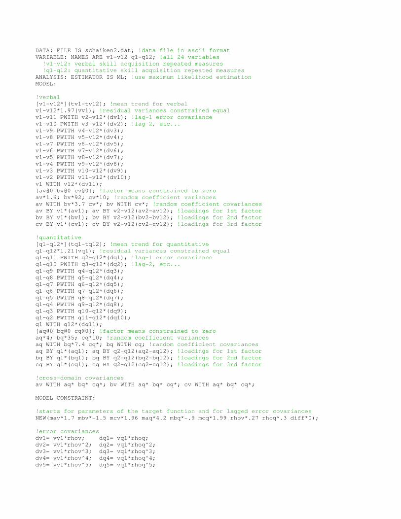
B WITH
C 0.000 0.000 999.000 999.000
M -0.026 0.016 -1.572 0.116 !COVARIANCE OF MAXIMIZER
!AND THETA1 RANDOM
C WITH !COEFFICIENTS
M 0.000 0.000 999.000 999.000
CONC1 WITH
CONC2 0.226 0.077 2.943 0.003 !LAG-1 ERROR COVARIANCE
!
CONC2 WITH !
CONC3 0.226 0.077 2.943 0.003 !
!
CONC3 WITH !
CONC4 0.226 0.077 2.943 0.003 !
!
CONC4 WITH !
CONC5 0.226 0.077 2.943 0.003 !
!
CONC5 WITH !
CONC6 0.226 0.077 2.943 0.003 !
!
CONC6 WITH !
CONC7 0.226 0.077 2.943 0.003 !
!
CONC7 WITH !
CONC8 0.226 0.077 2.943 0.003 !
!
CONC8 WITH !
CONC9 0.226 0.077 2.943 0.003 !
!
CONC9 WITH !
CONC10 0.226 0.077 2.943 0.003 !
!
CONC10 WITH !
CONC11 0.226 0.077 2.943 0.003 !
Means
B 0.000 0.000 999.000 999.000 !FACTOR MEANS FIXED = 0
C 0.000 0.000 999.000 999.000 !
M 0.000 0.000 999.000 999.000 !
Intercepts
CONC1 999.000 0.000 999.000 999.000
CONC2 999.000 0.000 999.000 999.000
CONC3 999.000 0.000 999.000 999.000
CONC4 999.000 0.000 999.000 999.000

CONC5 999.000 0.000 999.000 999.000
CONC6 999.000 0.000 999.000 999.000
CONC7 999.000 0.000 999.000 999.000
CONC8 999.000 0.000 999.000 999.000
CONC9 999.000 0.000 999.000 999.000
CONC10 999.000 0.000 999.000 999.000
CONC11 999.000 0.000 999.000 999.000
Variances
B 0.002 0.001 1.559 0.119 !VARIANCES OF THETA1,
C 0.000 0.000 999.000 999.000 !THETA2, AND MAXIMIZER
M 0.522 0.291 1.796 0.073 !COEFFICIENTS
Residual Variances
CONC1 0.731 0.119 6.119 0.000 !RESIDUAL VARIANCE, HELD
CONC2 0.731 0.119 6.119 0.000 !EQUAL OVER TIME
CONC3 0.731 0.119 6.119 0.000 !
CONC4 0.731 0.119 6.119 0.000 !
CONC5 0.731 0.119 6.119 0.000 !
CONC6 0.731 0.119 6.119 0.000 !
CONC7 0.731 0.119 6.119 0.000 !
CONC8 0.731 0.119 6.119 0.000 !
CONC9 0.731 0.119 6.119 0.000 !
CONC10 0.731 0.119 6.119 0.000 !
CONC11 0.731 0.119 6.119 0.000 !
New/Additional Parameters
MB 0.069 0.013 5.258 0.000 !MEAN THETA1 ESTIMATE
MC 0.017 0.001 14.672 0.000 !MEAN THETA2 ESTIMATE
MM 1.768 0.189 9.342 0.000 !MEAN MAXIMIZER ESTIMATE
QUALITY OF NUMERICAL RESULTS
Condition Number for the Information Matrix 0.496E-07
(ratio of smallest to largest eigenvalue)
10. Annotated output: unconditional bilinear spline model
Mplus VERSION 7.2
MUTHEN & MUTHEN
06/10/2014 5:36 PM
INPUT INSTRUCTIONS
TITLE: zerbe glucose;
DATA: FILE IS glucose.dat; !data file in ascii format
VARIABLE: NAMES ARE obese ph1-ph8; !all 9 variables
USEVARIABLES ARE ph1-ph8; !we plan to model 8 variables
!obese: obesity status, 0=control, 1=obese
!ph1-ph8: plasma phosphate concentration repeated measures
!ANALYSIS: BOOTSTRAP IS 1000; !for bootstrap confidence intervals if desired
MODEL:
[ph1-ph8*](z1-z8); !mean trend (z's defined below)
ph1-ph8*(ve); !residual variances constrained equal
w1-w4*; !random coefficient variances
w1 WITH w2*; w1 WITH w3*; w1 WITH w4*; !random coefficient covariances
w2 WITH w3*; w2 WITH w4*; w3 WITH w4*; !random coefficient covariances
[w1@0 w2@0 w3@0 w4@0]; !factor means constrained to zero
w1 BY ph1-ph8@1; !loadings for 1st factor, constrained to 1
w2 BY ph1*(w21); w2 BY ph2-ph8(w22-w28); !loadings for 2nd factor, defined below
w3 BY ph1*(w31); w3 BY ph2-ph8(w32-w38); !loadings for 3rd factor, defined below

w4 BY ph1*(w41); w4 BY ph2-ph8(w42-w48); !loadings for knot factor, defined below
MODEL CONSTRAINT:
!starts for parameters of the target function
NEW(mw1*3.4 mw2*-.26 mw3*.54 mw4*1.6 b1-b4);
!intercepts constrained equal to target function
z1=mw1+mw2*0.0+mw3*sqrt((0.0-mw4)^2);
z2=mw1+mw2*0.5+mw3*sqrt((0.5-mw4)^2);
z3=mw1+mw2*1.0+mw3*sqrt((1.0-mw4)^2);
z4=mw1+mw2*1.5+mw3*sqrt((1.5-mw4)^2);
z5=mw1+mw2*2.0+mw3*sqrt((2.0-mw4)^2);
z6=mw1+mw2*3.0+mw3*sqrt((3.0-mw4)^2);
z7=mw1+mw2*4.0+mw3*sqrt((4.0-mw4)^2);
z8=mw1+mw2*5.0+mw3*sqrt((5.0-mw4)^2);
!loadings for 2nd and 3rd factors, constrained to d(y)/d(mw2) and d(y)/d(mw3)
w21=0.0; w31=sqrt((0.0-mw4)^2);
w22=0.5; w32=sqrt((0.5-mw4)^2);
w23=1.0; w33=sqrt((1.0-mw4)^2);
w24=1.5; w34=sqrt((1.5-mw4)^2);
w25=2.0; w35=sqrt((2.0-mw4)^2);
w26=3.0; w36=sqrt((3.0-mw4)^2);
w27=4.0; w37=sqrt((4.0-mw4)^2);
w28=5.0; w38=sqrt((5.0-mw4)^2);
!loadings for knot factor, constrained to d(y)/d(mw4)
w41=(mw3*(mw4-0.0))/sqrt((0.0-mw4)^2);
w42=(mw3*(mw4-0.5))/sqrt((0.5-mw4)^2);
w43=(mw3*(mw4-1.0))/sqrt((1.0-mw4)^2);
w44=(mw3*(mw4-1.5))/sqrt((1.5-mw4)^2);
w45=(mw3*(mw4-2.0))/sqrt((2.0-mw4)^2);
w46=(mw3*(mw4-3.0))/sqrt((3.0-mw4)^2);
w47=(mw3*(mw4-4.0))/sqrt((4.0-mw4)^2);
w48=(mw3*(mw4-5.0))/sqrt((5.0-mw4)^2);
!parameters of original parameterization
b1=mw1+mw3*mw4;
b2=mw2-mw3;
b3=mw1-mw3*mw4;
b4=mw2+mw3;
OUTPUT: TECH1; !CINTERVAL(BCBOOTSTRAP);
INPUT READING TERMINATED NORMALLY
zerbe glucose;
SUMMARY OF ANALYSIS
Number of groups 1
Number of observations 33
Number of dependent variables 8
Number of independent variables 0
Number of continuous latent variables 4
Observed dependent variables
Continuous
PH1 PH2 PH3 PH4 PH5 PH6
PH7 PH8

Continuous latent variables
W1 W2 W3 W4
Estimator ML
Information matrix OBSERVED
Maximum number of iterations 1000
Convergence criterion 0.500D-04
Maximum number of steepest descent iterations 20
Input data file(s)
glucose.dat
Input data format FREE
THE MODEL ESTIMATION TERMINATED NORMALLY
MODEL FIT INFORMATION
Number of Free Parameters 15
Loglikelihood
H0 Value -176.244
H1 Value -142.162
Information Criteria
Akaike (AIC) 382.487
Bayesian (BIC) 404.935
Sample-Size Adjusted BIC 358.147
(n* = (n + 2) / 24)
Chi-Square Test of Model Fit
Value 68.163
Degrees of Freedom 29
P-Value 0.0001
RMSEA (Root Mean Square Error Of Approximation)
Estimate 0.202
90 Percent C.I. 0.140 0.265
Probability RMSEA <= .05 0.000
CFI/TLI
CFI 0.843
TLI 0.849
Chi-Square Test of Model Fit for the Baseline Model
Value 277.636
Degrees of Freedom 28
P-Value 0.0000
SRMR (Standardized Root Mean Square Residual)
Value 0.212
MODEL RESULTS
Two-Tailed

Estimate S.E. Est./S.E. P-Value
W1 BY
PH1 1.000 0.000 999.000 999.000
PH2 1.000 0.000 999.000 999.000
PH3 1.000 0.000 999.000 999.000
PH4 1.000 0.000 999.000 999.000
PH5 1.000 0.000 999.000 999.000
PH6 1.000 0.000 999.000 999.000
PH7 1.000 0.000 999.000 999.000
PH8 1.000 0.000 999.000 999.000
W2 BY
PH1 0.000 0.000 999.000 999.000
PH2 0.500 0.000 999.000 999.000
PH3 1.000 0.000 999.000 999.000
PH4 1.500 0.000 999.000 999.000
PH5 2.000 0.000 999.000 999.000
PH6 3.000 0.000 999.000 999.000
PH7 4.000 0.000 999.000 999.000
PH8 5.000 0.000 999.000 999.000
W3 BY
PH1 1.588 0.112 14.181 0.000
PH2 1.088 0.112 9.715 0.000
PH3 0.588 0.112 5.248 0.000
PH4 0.088 0.112 0.782 0.434
PH5 0.412 0.112 3.684 0.000
PH6 1.412 0.112 12.616 0.000
PH7 2.412 0.112 21.549 0.000
PH8 3.412 0.112 30.481 0.000
W4 BY
PH1 0.539 0.040 13.436 0.000
PH2 0.539 0.040 13.436 0.000
PH3 0.539 0.040 13.436 0.000
PH4 0.539 0.040 13.436 0.000
PH5 -0.539 0.040 -13.436 0.000
PH6 -0.539 0.040 -13.436 0.000
PH7 -0.539 0.040 -13.436 0.000
PH8 -0.539 0.040 -13.436 0.000
W1 WITH !COVARIANCES OF RANDOM
W2 -0.030 0.028 -1.064 0.287 !COEFFICIENTS
W3 -0.024 0.030 -0.810 0.418 !
W4 -0.008 0.085 -0.089 0.929 !
!
W2 WITH !
W3 -0.009 0.009 -1.028 0.304 !
W4 0.018 0.026 0.701 0.484 !
!
W3 WITH !
W4 0.001 0.027 0.036 0.971 !
Means
W1 0.000 0.000 999.000 999.000 !FACTOR MEANS FIXED = 0
W2 0.000 0.000 999.000 999.000 !
W3 0.000 0.000 999.000 999.000 !
W4 0.000 0.000 999.000 999.000 !
Intercepts
PH1 4.256 0.134 31.879 0.000
PH2 3.858 0.124 31.115 0.000

PH3 3.459 0.123 28.182 0.000
PH4 3.061 0.130 23.537 0.000
PH5 3.107 0.120 25.928 0.000
PH6 3.388 0.104 32.705 0.000
PH7 3.668 0.098 37.354 0.000
PH8 3.949 0.105 37.477 0.000
Variances
W1 0.457 0.135 3.397 0.001 !VARIANCES OF RANDOM
W2 0.013 0.010 1.291 0.197 !COEFFICIENTS
W3 0.027 0.013 2.029 0.042 !
W4 0.254 0.110 2.304 0.021 !
Residual Variances
PH1 0.103 0.013 8.124 0.000 !RESIDUAL VARIANCE, HELD EQUAL
PH2 0.103 0.013 8.124 0.000 !OVER TIME
PH3 0.103 0.013 8.124 0.000 !
PH4 0.103 0.013 8.124 0.000 !
PH5 0.103 0.013 8.124 0.000 !
PH6 0.103 0.013 8.124 0.000 !
PH7 0.103 0.013 8.124 0.000 !
PH8 0.103 0.013 8.124 0.000 !
New/Additional Parameters
MW1 3.400 0.128 26.470 0.000 !MEAN OF 1ST GROWTH PARAMETER
MW2 -0.258 0.034 -7.526 0.000 !MEAN OF 2ND GROWTH PARAMETER
MW3 0.539 0.040 13.436 0.000 !MEAN OF 3RD GROWTH PARAMETER
MW4 1.588 0.112 14.181 0.000 !MEAN OF KNOT PARAMETER
B1 4.256 0.134 31.879 0.000 !INTERCEPT FOR FIRST SEGMENT
B2 -0.797 0.066 -12.158 0.000 !SLOPE FOR FIRST SEGMENT
B3 2.545 0.171 14.881 0.000 !INTERCEPT FOR SECOND SEGMENT
B4 0.281 0.036 7.876 0.000 !SLOPE FOR SECOND SEGMENT
QUALITY OF NUMERICAL RESULTS
Condition Number for the Information Matrix 0.260E-05
(ratio of smallest to largest eigenvalue)
11. Annotated output: conditional bilinear spline model
Mplus VERSION 7.2
MUTHEN & MUTHEN
06/10/2014 5:37 PM
INPUT INSTRUCTIONS
TITLE: zerbe glucose;
DATA: FILE IS glucose.dat; !data file in ascii format
DEFINE: xobese=abs(obese-1); !1=control; 0=obese
VARIABLE: NAMES ARE obese ph1-ph8; !all 9 variables
!obese: obesity status, 0=control, 1=obese
!ph1-ph8: plasma phosphate concentration repeated measures
USEVARIABLES ARE ph1-ph8 xobese; !we plan to model 9 variables
!ANALYSIS: BOOTSTRAP IS 1000; !for bootstrap confidence intervals if desired
MODEL:
[ph1-ph8*](z1-z8); !mean trend (z's defined below)
ph1-ph8*(ve); !residual variances constrained equal
w1-w4*; !random coefficient residual variances
w1 WITH w2*; w1 WITH w3*; w1 WITH w4*; !random coefficient residual covariances
w2 WITH w3*; w2 WITH w4*; w3 WITH w4*; !random coefficient residual covariances
[w1@0 w2@0 w3@0 w4@0]; !factor intercepts constrained to zero

w1 BY ph1-ph8@1; !loadings for 1st factor, constrained to 1
w2 BY ph1*(w21); w2 BY ph2-ph8(w22-w28); !loadings for 2nd factor, defined below
w3 BY ph1*(w31); w3 BY ph2-ph8(w32-w38); !loadings for 3rd factor, defined below
w4 BY ph1*(w41); w4 BY ph2-ph8(w42-w48); !loadings for knot factor, defined below
w1-w4 ON xobese; !regress random coefficients on obese
MODEL CONSTRAINT:
!starts for parameters of the target function
NEW(mw1*3.5 mw2*-.21 mw3*.49 mw4*1.95 b1-b4);
!intercepts constrained equal to target function
z1=mw1+mw2*0.0+mw3*sqrt((0.0-mw4)^2);
z2=mw1+mw2*0.5+mw3*sqrt((0.5-mw4)^2);
z3=mw1+mw2*1.0+mw3*sqrt((1.0-mw4)^2);
z4=mw1+mw2*1.5+mw3*sqrt((1.5-mw4)^2);
z5=mw1+mw2*2.0+mw3*sqrt((2.0-mw4)^2);
z6=mw1+mw2*3.0+mw3*sqrt((3.0-mw4)^2);
z7=mw1+mw2*4.0+mw3*sqrt((4.0-mw4)^2);
z8=mw1+mw2*5.0+mw3*sqrt((5.0-mw4)^2);
!loadings for 2nd and 3rd factors, constrained to d(y)/d(mw2) and d(y)/d(mw3)
w21=0.0; w31=sqrt((0.0-mw4)^2);
w22=0.5; w32=sqrt((0.5-mw4)^2);
w23=1.0; w33=sqrt((1.0-mw4)^2);
w24=1.5; w34=sqrt((1.5-mw4)^2);
w25=2.0; w35=sqrt((2.0-mw4)^2);
w26=3.0; w36=sqrt((3.0-mw4)^2);
w27=4.0; w37=sqrt((4.0-mw4)^2);
w28=5.0; w38=sqrt((5.0-mw4)^2);
!loadings for knot factor, constrained to d(y)/d(mw4)
w41=(mw3*(mw4-0.0))/sqrt((0.0-mw4)^2);
w42=(mw3*(mw4-0.5))/sqrt((0.5-mw4)^2);
w43=(mw3*(mw4-1.0))/sqrt((1.0-mw4)^2);
w44=(mw3*(mw4-1.5))/sqrt((1.5-mw4)^2);
w45=(mw3*(mw4-2.0))/sqrt((2.0-mw4)^2);
w46=(mw3*(mw4-3.0))/sqrt((3.0-mw4)^2);
w47=(mw3*(mw4-4.0))/sqrt((4.0-mw4)^2);
w48=(mw3*(mw4-5.0))/sqrt((5.0-mw4)^2);
!parameters of original parameterization
b1=mw1+mw3*mw4;
b2=mw2-mw3;
b3=mw1-mw3*mw4;
b4=mw2+mw3;
OUTPUT: TECH1; !CINTERVAL(BCBOOTSTRAP);
INPUT READING TERMINATED NORMALLY
zerbe glucose;
SUMMARY OF ANALYSIS
Number of groups 1
Number of observations 33
Number of dependent variables 8
Number of independent variables 1
Number of continuous latent variables 4
Observed dependent variables

Continuous
PH1 PH2 PH3 PH4 PH5 PH6
PH7 PH8
Observed independent variables
XOBESE
Continuous latent variables
W1 W2 W3 W4
Estimator ML
Information matrix OBSERVED
Maximum number of iterations 1000
Convergence criterion 0.500D-04
Maximum number of steepest descent iterations 20
Input data file(s)
glucose.dat
Input data format FREE
THE MODEL ESTIMATION TERMINATED NORMALLY
MODEL FIT INFORMATION
Number of Free Parameters 19
Loglikelihood
H0 Value -161.967
H1 Value -126.612
Information Criteria
Akaike (AIC) 361.934
Bayesian (BIC) 390.368
Sample-Size Adjusted BIC 331.103
(n* = (n + 2) / 24)
Chi-Square Test of Model Fit
Value 70.711
Degrees of Freedom 33
P-Value 0.0001
RMSEA (Root Mean Square Error Of Approximation)
Estimate 0.186
90 Percent C.I. 0.126 0.246
Probability RMSEA <= .05 0.001
CFI/TLI
CFI 0.862
TLI 0.849
Chi-Square Test of Model Fit for the Baseline Model
Value 308.737
Degrees of Freedom 36
P-Value 0.0000
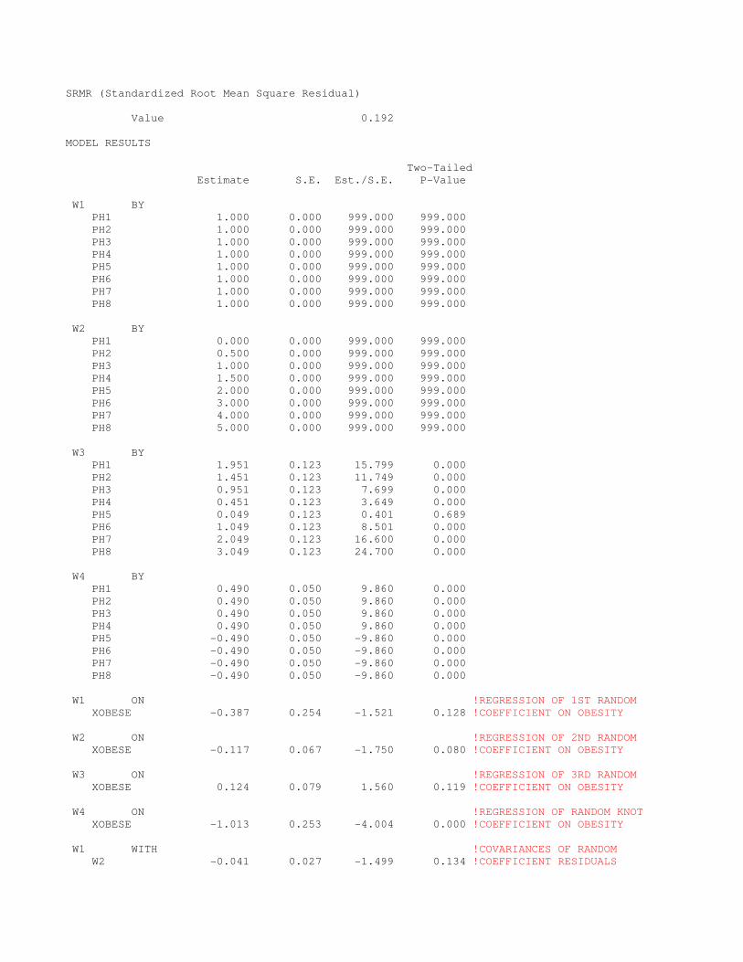
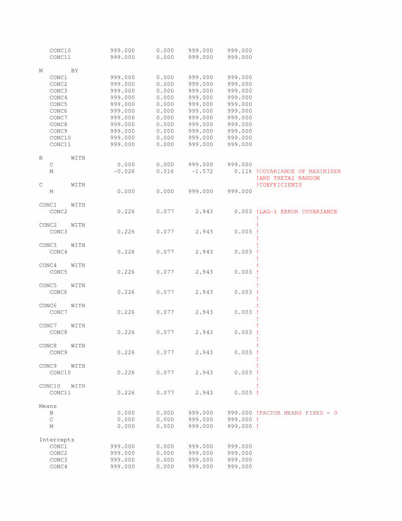
SRMR (Standardized Root Mean Square Residual)
Value 0.192
MODEL RESULTS
Two-Tailed
Estimate S.E. Est./S.E. P-Value
W1 BY
PH1 1.000 0.000 999.000 999.000
PH2 1.000 0.000 999.000 999.000
PH3 1.000 0.000 999.000 999.000
PH4 1.000 0.000 999.000 999.000
PH5 1.000 0.000 999.000 999.000
PH6 1.000 0.000 999.000 999.000
PH7 1.000 0.000 999.000 999.000
PH8 1.000 0.000 999.000 999.000
W2 BY
PH1 0.000 0.000 999.000 999.000
PH2 0.500 0.000 999.000 999.000
PH3 1.000 0.000 999.000 999.000
PH4 1.500 0.000 999.000 999.000
PH5 2.000 0.000 999.000 999.000
PH6 3.000 0.000 999.000 999.000
PH7 4.000 0.000 999.000 999.000
PH8 5.000 0.000 999.000 999.000
W3 BY
PH1 1.951 0.123 15.799 0.000
PH2 1.451 0.123 11.749 0.000
PH3 0.951 0.123 7.699 0.000
PH4 0.451 0.123 3.649 0.000
PH5 0.049 0.123 0.401 0.689
PH6 1.049 0.123 8.501 0.000
PH7 2.049 0.123 16.600 0.000
PH8 3.049 0.123 24.700 0.000
W4 BY
PH1 0.490 0.050 9.860 0.000
PH2 0.490 0.050 9.860 0.000
PH3 0.490 0.050 9.860 0.000
PH4 0.490 0.050 9.860 0.000
PH5 -0.490 0.050 -9.860 0.000
PH6 -0.490 0.050 -9.860 0.000
PH7 -0.490 0.050 -9.860 0.000
PH8 -0.490 0.050 -9.860 0.000
W1 ON !REGRESSION OF 1ST RANDOM
XOBESE -0.387 0.254 -1.521 0.128 !COEFFICIENT ON OBESITY
W2 ON !REGRESSION OF 2ND RANDOM
XOBESE -0.117 0.067 -1.750 0.080 !COEFFICIENT ON OBESITY
W3 ON !REGRESSION OF 3RD RANDOM
XOBESE 0.124 0.079 1.560 0.119 !COEFFICIENT ON OBESITY
W4 ON !REGRESSION OF RANDOM KNOT
XOBESE -1.013 0.253 -4.004 0.000 !COEFFICIENT ON OBESITY
W1 WITH !COVARIANCES OF RANDOM
W2 -0.041 0.027 -1.499 0.134 !COEFFICIENT RESIDUALS

W3 -0.013 0.028 -0.464 0.643 !
W4 -0.084 0.077 -1.093 0.274 !
!
W2 WITH !
W3 -0.006 0.008 -0.714 0.475 !
W4 -0.001 0.023 -0.061 0.951 !
!
W3 WITH !
W4 0.011 0.023 0.468 0.639 !
Intercepts
PH1 4.509 0.156 28.814 0.000
PH2 4.158 0.136 30.638 0.000
PH3 3.807 0.125 30.533 0.000
PH4 3.456 0.126 27.431 0.000
PH5 3.154 0.153 20.563 0.000
PH6 3.432 0.132 25.906 0.000
PH7 3.711 0.126 29.539 0.000
PH8 3.989 0.135 29.566 0.000
W1 0.000 0.000 999.000 999.000 !FACTOR INTERCEPTS FIXED = 0
W2 0.000 0.000 999.000 999.000 !
W3 0.000 0.000 999.000 999.000 !
W4 0.000 0.000 999.000 999.000 !
Residual Variances
PH1 0.103 0.013 8.124 0.000 !RESIDUAL VARIANCE, HELD EQUAL
PH2 0.103 0.013 8.124 0.000 !OVER TIME
PH3 0.103 0.013 8.124 0.000 !
PH4 0.103 0.013 8.124 0.000 !
PH5 0.103 0.013 8.124 0.000 !
PH6 0.103 0.013 8.124 0.000 !
PH7 0.103 0.013 8.124 0.000 !
PH8 0.103 0.013 8.124 0.000 !
W1 0.421 0.126 3.349 0.001 !RESIDUAL VARIANCES OF RANDOM
W2 0.010 0.009 1.043 0.297 !COEFFICIENTS
W3 0.024 0.013 1.879 0.060 !
W4 0.076 0.082 0.929 0.353 !
New/Additional Parameters
MW1 3.553 0.160 22.272 0.000 !CONDITIONAL MEANS OF ALL 4
MW2 -0.212 0.042 -5.026 0.000 !GROWTH PARAMETERS
MW3 0.490 0.050 9.860 0.000 !
MW4 1.951 0.123 15.799 0.000 !
B1 4.509 0.156 28.814 0.000 !CONDITIONAL MEANS OF ORIGINAL
B2 -0.702 0.080 -8.778 0.000 !INTERCEPTS AND SLOPES FOR
B3 2.596 0.219 11.845 0.000 !FIRST AND SECOND SEGMENTS
B4 0.278 0.046 6.080 0.000 !
QUALITY OF NUMERICAL RESULTS
Condition Number for the Information Matrix 0.308E-05
(ratio of smallest to largest eigenvalue)
12. Annotated output: negative exponential function with intercept, asymptote, and rate
Mplus VERSION 7.2
MUTHEN & MUTHEN
06/10/2014 5:55 PM
INPUT INSTRUCTIONS
TITLE: chaiken, negative exponential, original parameterization;

DATA: FILE IS schaiken2.dat; !data file in ascii format
VARIABLE: NAMES ARE v1-v12 q1-q12; !all 24 variables
!v1-v12: verbal skill acquisition repeated measures
!q1-q12: quantitative skill acquisition repeated measures
ANALYSIS: ESTIMATOR IS ML; !use maximum likelihood estimation
MODEL:
!verbal
[v1-v12*](tv1-tv12); !mean trend for verbal
v1-v12*1.97(vv1); !residual variances constrained equal
v1-v11 PWITH v2-v12*(dv1); !lag-1 error covariance
v1-v10 PWITH v3-v12*(dv2); !lag-2, etc...
v1-v9 PWITH v4-v12*(dv3);
v1-v8 PWITH v5-v12*(dv4);
v1-v7 PWITH v6-v12*(dv5);
v1-v6 PWITH v7-v12*(dv6);
v1-v5 PWITH v8-v12*(dv7);
v1-v4 PWITH v9-v12*(dv8);
v1-v3 PWITH v10-v12*(dv9);
v1-v2 PWITH v11-v12*(dv10);
v1 WITH v12*(dv11);
[av@0 bv@0 cv@0]; !factor means constrained to zero
av*; bv*; cv*; !random coefficient variances
av WITH bv* cv*; bv WITH cv*; !random coefficient covariances
av BY v1*(av1); av BY v2-v12(av2-av12); !loadings for 1st factor
bv BY v1*(bv1); bv BY v2-v12(bv2-bv12); !loadings for 2nd factor
cv BY v1*(cv1); cv BY v2-v12(cv2-cv12); !loadings for 3rd factor
!quantitative
[q1-q12*](tq1-tq12); !mean trend for quantitative
q1-q12*1.21(vq1); !residual variances constrained equal
q1-q11 PWITH q2-q12*(dq1); !lag-1 error covariance
q1-q10 PWITH q3-q12*(dq2); !lag-2, etc...
q1-q9 PWITH q4-q12*(dq3);
q1-q8 PWITH q5-q12*(dq4);
q1-q7 PWITH q6-q12*(dq5);
q1-q6 PWITH q7-q12*(dq6);
q1-q5 PWITH q8-q12*(dq7);
q1-q4 PWITH q9-q12*(dq8);
q1-q3 PWITH q10-q12*(dq9);
q1-q2 PWITH q11-q12*(dq10);
q1 WITH q12*(dq11);
[aq@0 bq@0 cq@0]; !factor means constrained to zero
aq*; bq*; cq*; !random coefficient variances
aq WITH bq* cq*; bq WITH cq; !random coefficient covariances
aq BY q1*(aq1); aq BY q2-q12(aq2-aq12); !loadings for 1st factor
bq BY q1*(bq1); bq BY q2-q12(bq2-bq12); !loadings for 2nd factor
cq BY q1*(cq1); cq BY q2-q12(cq2-cq12); !loadings for 3rd factor
!cross-domain covariances
av WITH aq* bq*; bv WITH aq* bq*;
MODEL CONSTRAINT:
!starts for parameters of the target function and for lagged error covariances
NEW(mav*6.8 mbv*21 mcv*.7 maq*8.6 mbq*16.5 mcq*.7 rhov*.27 rhoq*.31);
!error covariances
dv1= vv1*rhov; dq1= vq1*rhoq;
dv2= vv1*rhov^2; dq2= vq1*rhoq^2;
dv3= vv1*rhov^3; dq3= vq1*rhoq^3;
dv4= vv1*rhov^4; dq4= vq1*rhoq^4;
dv5= vv1*rhov^5; dq5= vq1*rhoq^5;

dv6= vv1*rhov^6; dq6= vq1*rhoq^6;
dv7= vv1*rhov^7; dq7= vq1*rhoq^7;
dv8= vv1*rhov^8; dq8= vq1*rhoq^8;
dv9= vv1*rhov^9; dq9= vq1*rhoq^9;
dv10=vv1*rhov^10; dq10=vq1*rhoq^10;
dv11=vv1*rhov^11; dq11=vq1*rhoq^11;
!verbal and quantitative intercepts constrained equal to target function
tv1 =mav-(mav-mbv)*exp(-1*mcv*( 1-1)); tq1 =maq-(maq-mbq)*exp(-1*mcq*( 1-1));
tv2 =mav-(mav-mbv)*exp(-1*mcv*( 2-1)); tq2 =maq-(maq-mbq)*exp(-1*mcq*( 2-1));
tv3 =mav-(mav-mbv)*exp(-1*mcv*( 3-1)); tq3 =maq-(maq-mbq)*exp(-1*mcq*( 3-1));
tv4 =mav-(mav-mbv)*exp(-1*mcv*( 4-1)); tq4 =maq-(maq-mbq)*exp(-1*mcq*( 4-1));
tv5 =mav-(mav-mbv)*exp(-1*mcv*( 5-1)); tq5 =maq-(maq-mbq)*exp(-1*mcq*( 5-1));
tv6 =mav-(mav-mbv)*exp(-1*mcv*( 6-1)); tq6 =maq-(maq-mbq)*exp(-1*mcq*( 6-1));
tv7 =mav-(mav-mbv)*exp(-1*mcv*( 7-1)); tq7 =maq-(maq-mbq)*exp(-1*mcq*( 7-1));
tv8 =mav-(mav-mbv)*exp(-1*mcv*( 8-1)); tq8 =maq-(maq-mbq)*exp(-1*mcq*( 8-1));
tv9 =mav-(mav-mbv)*exp(-1*mcv*( 9-1)); tq9 =maq-(maq-mbq)*exp(-1*mcq*( 9-1));
tv10=mav-(mav-mbv)*exp(-1*mcv*(10-1)); tq10=maq-(maq-mbq)*exp(-1*mcq*(10-1));
tv11=mav-(mav-mbv)*exp(-1*mcv*(11-1)); tq11=maq-(maq-mbq)*exp(-1*mcq*(11-1));
tv12=mav-(mav-mbv)*exp(-1*mcv*(12-1)); tq12=maq-(maq-mbq)*exp(-1*mcq*(12-1));
!loadings on 1st factor, constrained to d(y)/d(mav) and d(y)/d(maq)
av1 =1-exp(-1*mcv*( 1-1)); aq1 =1-exp(-1*mcq*( 1-1));
av2 =1-exp(-1*mcv*( 2-1)); aq2 =1-exp(-1*mcq*( 2-1));
av3 =1-exp(-1*mcv*( 3-1)); aq3 =1-exp(-1*mcq*( 3-1));
av4 =1-exp(-1*mcv*( 4-1)); aq4 =1-exp(-1*mcq*( 4-1));
av5 =1-exp(-1*mcv*( 5-1)); aq5 =1-exp(-1*mcq*( 5-1));
av6 =1-exp(-1*mcv*( 6-1)); aq6 =1-exp(-1*mcq*( 6-1));
av7 =1-exp(-1*mcv*( 7-1)); aq7 =1-exp(-1*mcq*( 7-1));
av8 =1-exp(-1*mcv*( 8-1)); aq8 =1-exp(-1*mcq*( 8-1));
av9 =1-exp(-1*mcv*( 9-1)); aq9 =1-exp(-1*mcq*( 9-1));
av10=1-exp(-1*mcv*(10-1)); aq10=1-exp(-1*mcq*(10-1));
av11=1-exp(-1*mcv*(11-1)); aq11=1-exp(-1*mcq*(11-1));
av12=1-exp(-1*mcv*(12-1)); aq12=1-exp(-1*mcq*(12-1));
!loadings on 2nd and 3rd factors for verbal, constrained to d(y)/d(mbv) and d(y)/d(mcv)
bv1 =exp(-1*mcv*( 1-1)); cv1 =(mav-mbv)*( 1-1)*exp(-1*mcv*( 1-1));
bv2 =exp(-1*mcv*( 2-1)); cv2 =(mav-mbv)*( 2-1)*exp(-1*mcv*( 2-1));
bv3 =exp(-1*mcv*( 3-1)); cv3 =(mav-mbv)*( 3-1)*exp(-1*mcv*( 3-1));
bv4 =exp(-1*mcv*( 4-1)); cv4 =(mav-mbv)*( 4-1)*exp(-1*mcv*( 4-1));
bv5 =exp(-1*mcv*( 5-1)); cv5 =(mav-mbv)*( 5-1)*exp(-1*mcv*( 5-1));
bv6 =exp(-1*mcv*( 6-1)); cv6 =(mav-mbv)*( 6-1)*exp(-1*mcv*( 6-1));
bv7 =exp(-1*mcv*( 7-1)); cv7 =(mav-mbv)*( 7-1)*exp(-1*mcv*( 7-1));
bv8 =exp(-1*mcv*( 8-1)); cv8 =(mav-mbv)*( 8-1)*exp(-1*mcv*( 8-1));
bv9 =exp(-1*mcv*( 9-1)); cv9 =(mav-mbv)*( 9-1)*exp(-1*mcv*( 9-1));
bv10=exp(-1*mcv*(10-1)); cv10=(mav-mbv)*(10-1)*exp(-1*mcv*(10-1));
bv11=exp(-1*mcv*(11-1)); cv11=(mav-mbv)*(11-1)*exp(-1*mcv*(11-1));
bv12=exp(-1*mcv*(12-1)); cv12=(mav-mbv)*(12-1)*exp(-1*mcv*(12-1));
!loadings on 2nd and 3rd factors for quant., constrained to d(y)/d(mbv) and d(y)/d(mcv)
bq1 =exp(-1*mcq*( 1-1)); cq1 =(maq-mbq)*( 1-1)*exp(-1*mcq*( 1-1));
bq2 =exp(-1*mcq*( 2-1)); cq2 =(maq-mbq)*( 2-1)*exp(-1*mcq*( 2-1));
bq3 =exp(-1*mcq*( 3-1)); cq3 =(maq-mbq)*( 3-1)*exp(-1*mcq*( 3-1));
bq4 =exp(-1*mcq*( 4-1)); cq4 =(maq-mbq)*( 4-1)*exp(-1*mcq*( 4-1));
bq5 =exp(-1*mcq*( 5-1)); cq5 =(maq-mbq)*( 5-1)*exp(-1*mcq*( 5-1));
bq6 =exp(-1*mcq*( 6-1)); cq6 =(maq-mbq)*( 6-1)*exp(-1*mcq*( 6-1));
bq7 =exp(-1*mcq*( 7-1)); cq7 =(maq-mbq)*( 7-1)*exp(-1*mcq*( 7-1));
bq8 =exp(-1*mcq*( 8-1)); cq8 =(maq-mbq)*( 8-1)*exp(-1*mcq*( 8-1));
bq9 =exp(-1*mcq*( 9-1)); cq9 =(maq-mbq)*( 9-1)*exp(-1*mcq*( 9-1));
bq10=exp(-1*mcq*(10-1)); cq10=(maq-mbq)*(10-1)*exp(-1*mcq*(10-1));
bq11=exp(-1*mcq*(11-1)); cq11=(maq-mbq)*(11-1)*exp(-1*mcq*(11-1));
bq12=exp(-1*mcq*(12-1)); cq12=(maq-mbq)*(12-1)*exp(-1*mcq*(12-1));

OUTPUT: TECH1 TECH4;
INPUT READING TERMINATED NORMALLY
chaiken, negative exponential, original parameterization;
SUMMARY OF ANALYSIS
Number of groups 1
Number of observations 228
Number of dependent variables 24
Number of independent variables 0
Number of continuous latent variables 6
Observed dependent variables
Continuous
V1 V2 V3 V4 V5 V6
V7 V8 V9 V10 V11 V12
Q1 Q2 Q3 Q4 Q5 Q6
Q7 Q8 Q9 Q10 Q11 Q12
Continuous latent variables
AV BV CV AQ BQ CQ
Estimator ML
Information matrix OBSERVED
Maximum number of iterations 1000
Convergence criterion 0.500D-04
Maximum number of steepest descent iterations 20
Input data file(s)
schaiken2.dat
Input data format FREE
THE MODEL ESTIMATION TERMINATED NORMALLY
MODEL FIT INFORMATION
Number of Free Parameters 31
Loglikelihood
H0 Value -10314.946
H1 Value -9097.350
Information Criteria
Akaike (AIC) 20691.891
Bayesian (BIC) 20798.201
Sample-Size Adjusted BIC 20699.952
(n* = (n + 2) / 24)
Chi-Square Test of Model Fit
Value 2435.191
Degrees of Freedom 293
P-Value 0.0000
RMSEA (Root Mean Square Error Of Approximation)

Estimate 0.179
90 Percent C.I. 0.173 0.186
Probability RMSEA <= .05 0.000
CFI/TLI
CFI 0.730
TLI 0.745
Chi-Square Test of Model Fit for the Baseline Model
Value 8204.815
Degrees of Freedom 276
P-Value 0.0000
SRMR (Standardized Root Mean Square Residual)
Value 0.218
MODEL RESULTS
Two-Tailed
Estimate S.E. Est./S.E. P-Value
AV BY
V1 0.000 0.000 999.000 999.000
V2 0.514 0.010 53.981 0.000
V3 0.763 0.009 82.480 0.000
V4 0.885 0.007 131.042 0.000
V5 0.944 0.004 215.555 0.000
V6 0.973 0.003 365.328 0.000
V7 0.987 0.002 634.904 0.000
V8 0.994 0.001 1126.553 0.000
V9 0.997 0.000 2033.343 0.000
V10 0.998 0.000 3721.911 0.000
V11 0.999 0.000 6892.175 0.000
V12 1.000 0.000 12886.546 0.000
BV BY
V1 1.000 0.000 999.000 999.000
V2 0.486 0.010 51.121 0.000
V3 0.237 0.009 25.561 0.000
V4 0.115 0.007 17.040 0.000
V5 0.056 0.004 12.780 0.000
V6 0.027 0.003 10.224 0.000
V7 0.013 0.002 8.520 0.000
V8 0.006 0.001 7.303 0.000
V9 0.003 0.000 6.390 0.000
V10 0.002 0.000 5.680 0.000
V11 0.001 0.000 5.112 0.000
V12 0.000 0.000 4.647 0.000
CV BY
V1 0.000 0.000 999.000 999.000
V2 -7.020 0.352 -19.949 0.000
V3 -6.829 0.422 -16.191 0.000
V4 -4.982 0.382 -13.039 0.000
V5 -3.231 0.302 -10.712 0.000
V6 -1.965 0.218 -9.012 0.000
V7 -1.147 0.148 -7.744 0.000
V8 -0.651 0.096 -6.772 0.000
V9 -0.362 0.060 -6.009 0.000
V10 -0.198 0.037 -5.395 0.000

V11 -0.107 0.022 -4.892 0.000
V12 -0.057 0.013 -4.474 0.000
AQ BY
Q1 0.000 0.000 999.000 999.000
Q2 0.502 0.012 43.058 0.000
Q3 0.752 0.012 64.796 0.000
Q4 0.877 0.009 101.169 0.000
Q5 0.939 0.006 163.257 0.000
Q6 0.970 0.004 271.095 0.000
Q7 0.985 0.002 461.203 0.000
Q8 0.992 0.001 800.636 0.000
Q9 0.996 0.001 1413.322 0.000
Q10 0.998 0.000 2529.599 0.000
Q11 0.999 0.000 4579.770 0.000
Q12 1.000 0.000 8371.340 0.000
BQ BY
Q1 1.000 0.000 999.000 999.000
Q2 0.498 0.012 42.642 0.000
Q3 0.248 0.012 21.321 0.000
Q4 0.123 0.009 14.214 0.000
Q5 0.061 0.006 10.661 0.000
Q6 0.030 0.004 8.528 0.000
Q7 0.015 0.002 7.107 0.000
Q8 0.008 0.001 6.092 0.000
Q9 0.004 0.001 5.330 0.000
Q10 0.002 0.000 4.738 0.000
Q11 0.001 0.000 4.264 0.000
Q12 0.000 0.000 3.877 0.000
CQ BY
Q1 0.000 0.000 999.000 999.000
Q2 -3.913 0.187 -20.931 0.000
Q3 -3.894 0.240 -16.220 0.000
Q4 -2.906 0.233 -12.481 0.000
Q5 -1.928 0.194 -9.932 0.000
Q6 -1.199 0.147 -8.177 0.000
Q7 -0.716 0.103 -6.922 0.000
Q8 -0.416 0.069 -5.988 0.000
Q9 -0.236 0.045 -5.270 0.000
Q10 -0.132 0.028 -4.702 0.000
Q11 -0.073 0.017 -4.243 0.000
Q12 -0.040 0.010 -3.864 0.000
AV WITH !COVARIANCES OF VERBAL (V) AND
BV 3.783 0.976 3.875 0.000 !QUANTITATIVE (Q) RANDOM
CV -0.147 0.059 -2.479 0.013 !COEFFICIENTS
AQ 1.664 0.235 7.097 0.000 !
BQ 2.051 0.606 3.384 0.001 !
!
BV WITH !
CV -0.468 0.391 -1.196 0.232 !
AQ 8.242 1.468 5.616 0.000 !
BQ 23.425 4.200 5.578 0.000 !
!
AQ WITH !
BQ 7.414 0.985 7.530 0.000 !
CQ -0.126 0.073 -1.733 0.083 !
CV -0.205 0.082 -2.484 0.013 !
!
BQ WITH !
CQ 0.540 0.204 2.647 0.008 !
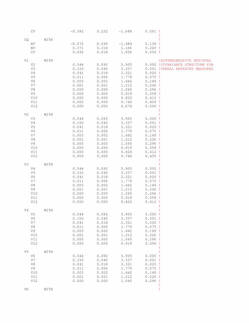
CV -0.392 0.232 -1.688 0.091 !
!
CQ WITH !
AV -0.072 0.049 -1.484 0.138 !
BV 0.371 0.318 1.166 0.243 !
CV 0.036 0.018 1.956 0.050 !
V1 WITH !AUTOREGRESSIVE RESIDUAL
V2 0.544 0.092 5.905 0.000 !COVARIANCE STRUCTURE FOR
V3 0.150 0.045 3.337 0.001 !VERBAL REPEATED MEASURES
V4 0.041 0.018 2.321 0.020 !
V5 0.011 0.006 1.779 0.075 !
V6 0.003 0.002 1.442 0.149 !
V7 0.001 0.001 1.212 0.226 !
V8 0.000 0.000 1.045 0.296 !
V9 0.000 0.000 0.919 0.358 !
V10 0.000 0.000 0.820 0.412 !
V11 0.000 0.000 0.740 0.459 !
V12 0.000 0.000 0.674 0.500 !
!
V2 WITH !
V3 0.544 0.092 5.905 0.000 !
V4 0.150 0.045 3.337 0.001 !
V5 0.041 0.018 2.321 0.020 !
V6 0.011 0.006 1.779 0.075 !
V7 0.003 0.002 1.442 0.149 !
V8 0.001 0.001 1.212 0.226 !
V9 0.000 0.000 1.045 0.296 !
V10 0.000 0.000 0.919 0.358 !
V11 0.000 0.000 0.820 0.412 !
V12 0.000 0.000 0.740 0.459 !
!
V3 WITH !
V4 0.544 0.092 5.905 0.000 !
V5 0.150 0.045 3.337 0.001 !
V6 0.041 0.018 2.321 0.020 !
V7 0.011 0.006 1.779 0.075 !
V8 0.003 0.002 1.442 0.149 !
V9 0.001 0.001 1.212 0.226 !
V10 0.000 0.000 1.045 0.296 !
V11 0.000 0.000 0.919 0.358 !
V12 0.000 0.000 0.820 0.412 !
!
V4 WITH !
V5 0.544 0.092 5.905 0.000 !
V6 0.150 0.045 3.337 0.001 !
V7 0.041 0.018 2.321 0.020 !
V8 0.011 0.006 1.779 0.075 !
V9 0.003 0.002 1.442 0.149 !
V10 0.001 0.001 1.212 0.226 !
V11 0.000 0.000 1.045 0.296 !
V12 0.000 0.000 0.919 0.358 !
!
V5 WITH !
V6 0.544 0.092 5.905 0.000 !
V7 0.150 0.045 3.337 0.001 !
V8 0.041 0.018 2.321 0.020 !
V9 0.011 0.006 1.779 0.075 !
V10 0.003 0.002 1.442 0.149 !
V11 0.001 0.001 1.212 0.226 !
V12 0.000 0.000 1.045 0.296 !
!
V6 WITH !

V7 0.544 0.092 5.905 0.000 !
V8 0.150 0.045 3.337 0.001 !
V9 0.041 0.018 2.321 0.020 !
V10 0.011 0.006 1.779 0.075 !
V11 0.003 0.002 1.442 0.149 !
V12 0.001 0.001 1.212 0.226 !
!
V7 WITH !
V8 0.544 0.092 5.905 0.000 !
V9 0.150 0.045 3.337 0.001 !
V10 0.041 0.018 2.321 0.020 !
V11 0.011 0.006 1.779 0.075 !
V12 0.003 0.002 1.442 0.149 !
!
V8 WITH !
V9 0.544 0.092 5.905 0.000 !
V10 0.150 0.045 3.337 0.001 !
V11 0.041 0.018 2.321 0.020 !
V12 0.011 0.006 1.779 0.075 !
!
V9 WITH !
V10 0.544 0.092 5.905 0.000 !
V11 0.150 0.045 3.337 0.001 !
V12 0.041 0.018 2.321 0.020 !
!
V10 WITH !
V11 0.544 0.092 5.905 0.000 !
V12 0.150 0.045 3.337 0.001 !
!
V11 WITH !
V12 0.544 0.092 5.905 0.000 !
Q1 WITH !AUTOREGRESSIVE RESIDUAL
Q2 0.345 0.053 6.528 0.000 !COVARIANCE STRUCTURE FOR
Q3 0.107 0.028 3.787 0.000 !QUANTITATIVE REPEATED MEASURES
Q4 0.033 0.012 2.662 0.008 !
Q5 0.010 0.005 2.051 0.040 !
Q6 0.003 0.002 1.668 0.095 !
Q7 0.001 0.001 1.405 0.160 !
Q8 0.000 0.000 1.214 0.225 !
Q9 0.000 0.000 1.068 0.285 !
Q10 0.000 0.000 0.954 0.340 !
Q11 0.000 0.000 0.862 0.389 !
Q12 0.000 0.000 0.786 0.432 !
!
Q2 WITH !
Q3 0.345 0.053 6.528 0.000 !
Q4 0.107 0.028 3.787 0.000 !
Q5 0.033 0.012 2.662 0.008 !
Q6 0.010 0.005 2.051 0.040 !
Q7 0.003 0.002 1.668 0.095 !
Q8 0.001 0.001 1.405 0.160 !
Q9 0.000 0.000 1.214 0.225 !
Q10 0.000 0.000 1.068 0.285 !
Q11 0.000 0.000 0.954 0.340 !
Q12 0.000 0.000 0.862 0.389 !
!
Q3 WITH !
Q4 0.345 0.053 6.528 0.000 !
Q5 0.107 0.028 3.787 0.000 !
Q6 0.033 0.012 2.662 0.008 !
Q7 0.010 0.005 2.051 0.040 !
Q8 0.003 0.002 1.668 0.095 !

Q9 0.001 0.001 1.405 0.160 !
Q10 0.000 0.000 1.214 0.225 !
Q11 0.000 0.000 1.068 0.285 !
Q12 0.000 0.000 0.954 0.340 !
!
Q4 WITH !
Q5 0.345 0.053 6.528 0.000 !
Q6 0.107 0.028 3.787 0.000 !
Q7 0.033 0.012 2.662 0.008 !
Q8 0.010 0.005 2.051 0.040 !
Q9 0.003 0.002 1.668 0.095 !
Q10 0.001 0.001 1.405 0.160 !
Q11 0.000 0.000 1.214 0.225 !
Q12 0.000 0.000 1.068 0.285 !
!
Q5 WITH !
Q6 0.345 0.053 6.528 0.000 !
Q7 0.107 0.028 3.787 0.000 !
Q8 0.033 0.012 2.662 0.008 !
Q9 0.010 0.005 2.051 0.040 !
Q10 0.003 0.002 1.668 0.095 !
Q11 0.001 0.001 1.405 0.160 !
Q12 0.000 0.000 1.214 0.225 !
!
Q6 WITH !
Q7 0.345 0.053 6.528 0.000 !
Q8 0.107 0.028 3.787 0.000 !
Q9 0.033 0.012 2.662 0.008 !
Q10 0.010 0.005 2.051 0.040 !
Q11 0.003 0.002 1.668 0.095 !
Q12 0.001 0.001 1.405 0.160 !
!
Q7 WITH !
Q8 0.345 0.053 6.528 0.000 !
Q9 0.107 0.028 3.787 0.000 !
Q10 0.033 0.012 2.662 0.008 !
Q11 0.010 0.005 2.051 0.040 !
Q12 0.003 0.002 1.668 0.095 !
!
Q8 WITH !
Q9 0.345 0.053 6.528 0.000 !
Q10 0.107 0.028 3.787 0.000 !
Q11 0.033 0.012 2.662 0.008 !
Q12 0.010 0.005 2.051 0.040 !
!
Q9 WITH !
Q10 0.345 0.053 6.528 0.000 !
Q11 0.107 0.028 3.787 0.000 !
Q12 0.033 0.012 2.662 0.008 !
!
Q10 WITH !
Q11 0.345 0.053 6.528 0.000 !
Q12 0.107 0.028 3.787 0.000 !
!
Q11 WITH !
Q12 0.345 0.053 6.528 0.000 !
Means
AV 0.000 0.000 999.000 999.000 !FACTOR MEANS FIXED = 0
BV 0.000 0.000 999.000 999.000 !
CV 0.000 0.000 999.000 999.000 !
AQ 0.000 0.000 999.000 999.000 !
BQ 0.000 0.000 999.000 999.000 !

CQ 0.000 0.000 999.000 999.000 !
Intercepts
V1 21.278 0.661 32.192 0.000
V2 13.865 0.374 37.074 0.000
V3 10.260 0.238 43.076 0.000
V4 8.506 0.164 51.793 0.000
V5 7.653 0.126 60.760 0.000
V6 7.238 0.109 66.405 0.000
V7 7.036 0.103 68.566 0.000
V8 6.938 0.101 69.035 0.000
V9 6.890 0.100 68.996 0.000
V10 6.867 0.100 68.879 0.000
V11 6.856 0.100 68.789 0.000
V12 6.850 0.100 68.733 0.000
Q1 16.492 0.404 40.778 0.000
Q2 12.541 0.261 47.962 0.000
Q3 10.575 0.202 52.297 0.000
Q4 9.597 0.171 56.083 0.000
Q5 9.111 0.155 58.658 0.000
Q6 8.868 0.148 59.868 0.000
Q7 8.748 0.145 60.270 0.000
Q8 8.688 0.144 60.347 0.000
Q9 8.658 0.144 60.330 0.000
Q10 8.643 0.143 60.299 0.000
Q11 8.636 0.143 60.275 0.000
Q12 8.632 0.143 60.261 0.000
Variances
AV 1.652 0.207 7.981 0.000 !VARIANCES OF RANDOM
BV 92.144 8.816 10.452 0.000 !COEFFICIENTS
CV 0.272 0.044 6.232 0.000 !
AQ 4.187 0.423 9.908 0.000 !
BQ 35.772 3.456 10.351 0.000 !
CQ 0.179 0.030 6.058 0.000 !
Residual Variances
V1 1.974 0.092 21.355 0.000 !VERBAL RESIDUAL VARIANCE
V2 1.974 0.092 21.355 0.000 !HELD EQUAL OVER TIME
V3 1.974 0.092 21.355 0.000 !
V4 1.974 0.092 21.355 0.000 !
V5 1.974 0.092 21.355 0.000 !
V6 1.974 0.092 21.355 0.000 !
V7 1.974 0.092 21.355 0.000 !
V8 1.974 0.092 21.355 0.000 !
V9 1.974 0.092 21.355 0.000 !
V10 1.974 0.092 21.355 0.000 !
V11 1.974 0.092 21.355 0.000 !
V12 1.974 0.092 21.355 0.000 !
Q1 1.112 0.055 20.403 0.000 !QUANTITATIVE RESIDUAL VARIANCE
Q2 1.112 0.055 20.403 0.000 !HELD EQUAL OVER TIME
Q3 1.112 0.055 20.403 0.000 !
Q4 1.112 0.055 20.403 0.000 !
Q5 1.112 0.055 20.403 0.000 !
Q6 1.112 0.055 20.403 0.000 !
Q7 1.112 0.055 20.403 0.000 !
Q8 1.112 0.055 20.403 0.000 !
Q9 1.112 0.055 20.403 0.000 !
Q10 1.112 0.055 20.403 0.000 !
Q11 1.112 0.055 20.403 0.000 !
Q12 1.112 0.055 20.403 0.000 !
New/Additional Parameters

MAV 6.845 0.100 68.667 0.000 !VERBAL MEAN ASYMPTOTE
MBV 21.278 0.661 32.192 0.000 !VERBAL MEAN INITIAL VALUE
MCV 0.721 0.020 36.845 0.000 !VERBAL MEAN RATE PARAMETER
MAQ 8.629 0.143 60.242 0.000 !QUANT. MEAN ASYMPTOTE
MBQ 16.492 0.404 40.778 0.000 !QUANT. MEAN INITIAL VALUE
MCQ 0.698 0.023 29.765 0.000 !QUANT. MEAN RATE PARAMETER
RHOV 0.276 0.036 7.597 0.000 !AUTOREGRESSIVE PARAMETER (V)
RHOQ 0.310 0.035 8.910 0.000 !AUTOREGRESSIVE PARAMETER (Q)
QUALITY OF NUMERICAL RESULTS
Condition Number for the Information Matrix 0.168E-03
(ratio of smallest to largest eigenvalue)
13. Annotated output: negative exponential function with intercept, half-life, and ARC
Mplus VERSION 7.2
MUTHEN & MUTHEN
06/10/2014 5:55 PM
INPUT INSTRUCTIONS
TITLE: chaiken, negative exponential with halflife and arc;
DATA: FILE IS schaiken2.dat; !data file in ascii format
VARIABLE: NAMES ARE v1-v12 q1-q12; !all 24 variables
!v1-v12: verbal skill acquisition repeated measures
!q1-q12: quantitative skill acquisition repeated measures
ANALYSIS: ESTIMATOR IS ML; !use maximum likelihood estimation
MODEL:
!verbal
[v1-v12*](tv1-tv12); !mean trend for verbal
v1-v12*1.97(vv1); !residual variances constrained equal
v1-v11 PWITH v2-v12*(dv1); !lag-1 error covariance
v1-v10 PWITH v3-v12*(dv2); !lag-2, etc...
v1-v9 PWITH v4-v12*(dv3);
v1-v8 PWITH v5-v12*(dv4);
v1-v7 PWITH v6-v12*(dv5);
v1-v6 PWITH v7-v12*(dv6);
v1-v5 PWITH v8-v12*(dv7);
v1-v4 PWITH v9-v12*(dv8);
v1-v3 PWITH v10-v12*(dv9);
v1-v2 PWITH v11-v12*(dv10);
v1 WITH v12*(dv11);
[av@0 bv@0 cv@0]; !factor means constrained to zero
av*1.6; bv*92; cv*10; !random coefficient variances
av WITH bv*3.7 cv*; bv WITH cv*; !random coefficient covariances
av BY v1*(av1); av BY v2-v12(av2-av12); !loadings for 1st factor
bv BY v1*(bv1); bv BY v2-v12(bv2-bv12); !loadings for 2nd factor
cv BY v1*(cv1); cv BY v2-v12(cv2-cv12); !loadings for 3rd factor
!quantitative
[q1-q12*](tq1-tq12); !mean trend for quantitative
q1-q12*1.21(vq1); !residual variances constrained equal
q1-q11 PWITH q2-q12*(dq1); !lag-1 error covariance
q1-q10 PWITH q3-q12*(dq2); !lag-2, etc...
q1-q9 PWITH q4-q12*(dq3);
q1-q8 PWITH q5-q12*(dq4);
q1-q7 PWITH q6-q12*(dq5);
q1-q6 PWITH q7-q12*(dq6);
q1-q5 PWITH q8-q12*(dq7);

q1-q4 PWITH q9-q12*(dq8);
q1-q3 PWITH q10-q12*(dq9);
q1-q2 PWITH q11-q12*(dq10);
q1 WITH q12*(dq11);
[aq@0 bq@0 cq@0]; !factor means constrained to zero
aq*4; bq*35; cq*10; !random coefficient variances
aq WITH bq*7.4 cq*; bq WITH cq; !random coefficient covariances
aq BY q1*(aq1); aq BY q2-q12(aq2-aq12); !loadings for 1st factor
bq BY q1*(bq1); bq BY q2-q12(bq2-bq12); !loadings for 2nd factor
cq BY q1*(cq1); cq BY q2-q12(cq2-cq12); !loadings for 3rd factor
!cross-domain covariances
av WITH aq* bq* cq*; bv WITH aq* bq* cq*; cv WITH aq* bq* cq*;
MODEL CONSTRAINT:
!starts for parameters of the target function and for lagged error covariances
NEW(mav*1.7 mbv*-1.5 mcv*1.96 maq*4.2 mbq*-.9 mcq*1.99 rhov*.27 rhoq*.3 diff*0);
!error covariances
dv1= vv1*rhov; dq1= vq1*rhoq;
dv2= vv1*rhov^2; dq2= vq1*rhoq^2;
dv3= vv1*rhov^3; dq3= vq1*rhoq^3;
dv4= vv1*rhov^4; dq4= vq1*rhoq^4;
dv5= vv1*rhov^5; dq5= vq1*rhoq^5;
dv6= vv1*rhov^6; dq6= vq1*rhoq^6;
dv7= vv1*rhov^7; dq7= vq1*rhoq^7;
dv8= vv1*rhov^8; dq8= vq1*rhoq^8;
dv9= vv1*rhov^9; dq9= vq1*rhoq^9;
dv10=vv1*rhov^10; dq10=vq1*rhoq^10;
dv11=vv1*rhov^11; dq11=vq1*rhoq^11;
!verbal intercepts constrained equal to target function
tv1 =mav+(mbv*11*(.5^(( 1-1)/(mcv-1))))/((.5^(11/(mcv-1)))-1);
tv2 =mav+(mbv*11*(.5^(( 2-1)/(mcv-1))))/((.5^(11/(mcv-1)))-1);
tv3 =mav+(mbv*11*(.5^(( 3-1)/(mcv-1))))/((.5^(11/(mcv-1)))-1);
tv4 =mav+(mbv*11*(.5^(( 4-1)/(mcv-1))))/((.5^(11/(mcv-1)))-1);
tv5 =mav+(mbv*11*(.5^(( 5-1)/(mcv-1))))/((.5^(11/(mcv-1)))-1);
tv6 =mav+(mbv*11*(.5^(( 6-1)/(mcv-1))))/((.5^(11/(mcv-1)))-1);
tv7 =mav+(mbv*11*(.5^(( 7-1)/(mcv-1))))/((.5^(11/(mcv-1)))-1);
tv8 =mav+(mbv*11*(.5^(( 8-1)/(mcv-1))))/((.5^(11/(mcv-1)))-1);
tv9 =mav+(mbv*11*(.5^(( 9-1)/(mcv-1))))/((.5^(11/(mcv-1)))-1);
tv10=mav+(mbv*11*(.5^((10-1)/(mcv-1))))/((.5^(11/(mcv-1)))-1);
tv11=mav+(mbv*11*(.5^((11-1)/(mcv-1))))/((.5^(11/(mcv-1)))-1);
tv12=mav+(mbv*11*(.5^((12-1)/(mcv-1))))/((.5^(11/(mcv-1)))-1);
!loadings on 1st factor, constrained to d(y)/d(mav) and d(y)/d(maq)
0=1-av1 ; 0=1-aq1 ;
0=1-av2 ; 0=1-aq2 ;
0=1-av3 ; 0=1-aq3 ;
0=1-av4 ; 0=1-aq4 ;
0=1-av5 ; 0=1-aq5 ;
0=1-av6 ; 0=1-aq6 ;
0=1-av7 ; 0=1-aq7 ;
0=1-av8 ; 0=1-aq8 ;
0=1-av9 ; 0=1-aq9 ;
0=1-av10; 0=1-aq10;
0=1-av11; 0=1-aq11;
0=1-av12; 0=1-aq12;
!loadings on 2nd factor for verbal, constrained to d(y)/d(mbv)
bv1 =(11*(.5^(( 1-1)/(mcv-1))))/((.5^(11/(mcv-1)))-1);
bv2 =(11*(.5^(( 2-1)/(mcv-1))))/((.5^(11/(mcv-1)))-1);

bv3 =(11*(.5^(( 3-1)/(mcv-1))))/((.5^(11/(mcv-1)))-1);
bv4 =(11*(.5^(( 4-1)/(mcv-1))))/((.5^(11/(mcv-1)))-1);
bv5 =(11*(.5^(( 5-1)/(mcv-1))))/((.5^(11/(mcv-1)))-1);
bv6 =(11*(.5^(( 6-1)/(mcv-1))))/((.5^(11/(mcv-1)))-1);
bv7 =(11*(.5^(( 7-1)/(mcv-1))))/((.5^(11/(mcv-1)))-1);
bv8 =(11*(.5^(( 8-1)/(mcv-1))))/((.5^(11/(mcv-1)))-1);
bv9 =(11*(.5^(( 9-1)/(mcv-1))))/((.5^(11/(mcv-1)))-1);
bv10=(11*(.5^((10-1)/(mcv-1))))/((.5^(11/(mcv-1)))-1);
bv11=(11*(.5^((11-1)/(mcv-1))))/((.5^(11/(mcv-1)))-1);
bv12=(11*(.5^((12-1)/(mcv-1))))/((.5^(11/(mcv-1)))-1);
!loadings on 3rd factor for verbal, constrained to d(y)/d(mcv)
cv1 =(.5^( 1/(mcv-1))*mcv*((.5^(1/(mcv-1)))*( 1-1)+(.5^(12/(mcv-1)))*(12- 1))*11*ln(.5))/
(((mcv-1)^2)*(((.5^(11/(mcv-1)))-(.5^(1/(mcv-1))))^2));
cv2 =(.5^( 2/(mcv-1))*mcv*((.5^(1/(mcv-1)))*( 2-1)+(.5^(12/(mcv-1)))*(12- 2))*11*ln(.5))/
(((mcv-1)^2)*(((.5^(11/(mcv-1)))-(.5^(1/(mcv-1))))^2));
cv3 =(.5^( 3/(mcv-1))*mcv*((.5^(1/(mcv-1)))*( 3-1)+(.5^(12/(mcv-1)))*(12- 3))*11*ln(.5))/
(((mcv-1)^2)*(((.5^(11/(mcv-1)))-(.5^(1/(mcv-1))))^2));
cv4 =(.5^( 4/(mcv-1))*mcv*((.5^(1/(mcv-1)))*( 4-1)+(.5^(12/(mcv-1)))*(12- 4))*11*ln(.5))/
(((mcv-1)^2)*(((.5^(11/(mcv-1)))-(.5^(1/(mcv-1))))^2));
cv5 =(.5^( 5/(mcv-1))*mcv*((.5^(1/(mcv-1)))*( 5-1)+(.5^(12/(mcv-1)))*(12- 5))*11*ln(.5))/
(((mcv-1)^2)*(((.5^(11/(mcv-1)))-(.5^(1/(mcv-1))))^2));
cv6 =(.5^( 6/(mcv-1))*mcv*((.5^(1/(mcv-1)))*( 6-1)+(.5^(12/(mcv-1)))*(12- 6))*11*ln(.5))/
(((mcv-1)^2)*(((.5^(11/(mcv-1)))-(.5^(1/(mcv-1))))^2));
cv7 =(.5^( 7/(mcv-1))*mcv*((.5^(1/(mcv-1)))*( 7-1)+(.5^(12/(mcv-1)))*(12- 7))*11*ln(.5))/
(((mcv-1)^2)*(((.5^(11/(mcv-1)))-(.5^(1/(mcv-1))))^2));
cv8 =(.5^( 8/(mcv-1))*mcv*((.5^(1/(mcv-1)))*( 8-1)+(.5^(12/(mcv-1)))*(12- 8))*11*ln(.5))/
(((mcv-1)^2)*(((.5^(11/(mcv-1)))-(.5^(1/(mcv-1))))^2));
cv9 =(.5^( 9/(mcv-1))*mcv*((.5^(1/(mcv-1)))*( 9-1)+(.5^(12/(mcv-1)))*(12- 9))*11*ln(.5))/
(((mcv-1)^2)*(((.5^(11/(mcv-1)))-(.5^(1/(mcv-1))))^2));
cv10=(.5^(10/(mcv-1))*mcv*((.5^(1/(mcv-1)))*(10-1)+(.5^(12/(mcv-1)))*(12-10))*11*ln(.5))/
(((mcv-1)^2)*(((.5^(11/(mcv-1)))-(.5^(1/(mcv-1))))^2));
cv11=(.5^(11/(mcv-1))*mcv*((.5^(1/(mcv-1)))*(11-1)+(.5^(12/(mcv-1)))*(12-11))*11*ln(.5))/
(((mcv-1)^2)*(((.5^(11/(mcv-1)))-(.5^(1/(mcv-1))))^2));
cv12=(.5^(12/(mcv-1))*mcv*((.5^(1/(mcv-1)))*(12-1)+(.5^(12/(mcv-1)))*(12-12))*11*ln(.5))/
(((mcv-1)^2)*(((.5^(11/(mcv-1)))-(.5^(1/(mcv-1))))^2));
!quantitative intercepts constrained equal to target function
tq1 =maq+(mbq*11*(.5^(( 1-1)/(mcq-1))))/((.5^(11/(mcq-1)))-1);
tq2 =maq+(mbq*11*(.5^(( 2-1)/(mcq-1))))/((.5^(11/(mcq-1)))-1);
tq3 =maq+(mbq*11*(.5^(( 3-1)/(mcq-1))))/((.5^(11/(mcq-1)))-1);
tq4 =maq+(mbq*11*(.5^(( 4-1)/(mcq-1))))/((.5^(11/(mcq-1)))-1);
tq5 =maq+(mbq*11*(.5^(( 5-1)/(mcq-1))))/((.5^(11/(mcq-1)))-1);
tq6 =maq+(mbq*11*(.5^(( 6-1)/(mcq-1))))/((.5^(11/(mcq-1)))-1);
tq7 =maq+(mbq*11*(.5^(( 7-1)/(mcq-1))))/((.5^(11/(mcq-1)))-1);
tq8 =maq+(mbq*11*(.5^(( 8-1)/(mcq-1))))/((.5^(11/(mcq-1)))-1);
tq9 =maq+(mbq*11*(.5^(( 9-1)/(mcq-1))))/((.5^(11/(mcq-1)))-1);
tq10=maq+(mbq*11*(.5^((10-1)/(mcq-1))))/((.5^(11/(mcq-1)))-1);
tq11=maq+(mbq*11*(.5^((11-1)/(mcq-1))))/((.5^(11/(mcq-1)))-1);
tq12=maq+(mbq*11*(.5^((12-1)/(mcq-1))))/((.5^(11/(mcq-1)))-1);
!loadings on 2nd factor for quantitative, constrained to d(y)/d(mbv)
bq1 =(11*(.5^(( 1-1)/(mcq-1))))/((.5^(11/(mcq-1)))-1);
bq2 =(11*(.5^(( 2-1)/(mcq-1))))/((.5^(11/(mcq-1)))-1);
bq3 =(11*(.5^(( 3-1)/(mcq-1))))/((.5^(11/(mcq-1)))-1);
bq4 =(11*(.5^(( 4-1)/(mcq-1))))/((.5^(11/(mcq-1)))-1);
bq5 =(11*(.5^(( 5-1)/(mcq-1))))/((.5^(11/(mcq-1)))-1);
bq6 =(11*(.5^(( 6-1)/(mcq-1))))/((.5^(11/(mcq-1)))-1);
bq7 =(11*(.5^(( 7-1)/(mcq-1))))/((.5^(11/(mcq-1)))-1);
bq8 =(11*(.5^(( 8-1)/(mcq-1))))/((.5^(11/(mcq-1)))-1);
bq9 =(11*(.5^(( 9-1)/(mcq-1))))/((.5^(11/(mcq-1)))-1);
bq10=(11*(.5^((10-1)/(mcq-1))))/((.5^(11/(mcq-1)))-1);
bq11=(11*(.5^((11-1)/(mcq-1))))/((.5^(11/(mcq-1)))-1);

bq12=(11*(.5^((12-1)/(mcq-1))))/((.5^(11/(mcq-1)))-1);
!loadings on 3rd factor for quantitative, constrained to d(y)/d(mcv)
cq1 =(.5^( 1/(mcq-1))*mcq*((.5^(1/(mcq-1)))*( 1-1)+(.5^(12/(mcq-1)))*(12- 1))*11*ln(.5))/
(((mcq-1)^2)*(((.5^(11/(mcq-1)))-(.5^(1/(mcq-1))))^2));
cq2 =(.5^( 2/(mcq-1))*mcq*((.5^(1/(mcq-1)))*( 2-1)+(.5^(12/(mcq-1)))*(12- 2))*11*ln(.5))/
(((mcq-1)^2)*(((.5^(11/(mcq-1)))-(.5^(1/(mcq-1))))^2));
cq3 =(.5^( 3/(mcq-1))*mcq*((.5^(1/(mcq-1)))*( 3-1)+(.5^(12/(mcq-1)))*(12- 3))*11*ln(.5))/
(((mcq-1)^2)*(((.5^(11/(mcq-1)))-(.5^(1/(mcq-1))))^2));
cq4 =(.5^( 4/(mcq-1))*mcq*((.5^(1/(mcq-1)))*( 4-1)+(.5^(12/(mcq-1)))*(12- 4))*11*ln(.5))/
(((mcq-1)^2)*(((.5^(11/(mcq-1)))-(.5^(1/(mcq-1))))^2));
cq5 =(.5^( 5/(mcq-1))*mcq*((.5^(1/(mcq-1)))*( 5-1)+(.5^(12/(mcq-1)))*(12- 5))*11*ln(.5))/
(((mcq-1)^2)*(((.5^(11/(mcq-1)))-(.5^(1/(mcq-1))))^2));
cq6 =(.5^( 6/(mcq-1))*mcq*((.5^(1/(mcq-1)))*( 6-1)+(.5^(12/(mcq-1)))*(12- 6))*11*ln(.5))/
(((mcq-1)^2)*(((.5^(11/(mcq-1)))-(.5^(1/(mcq-1))))^2));
cq7 =(.5^( 7/(mcq-1))*mcq*((.5^(1/(mcq-1)))*( 7-1)+(.5^(12/(mcq-1)))*(12- 7))*11*ln(.5))/
(((mcq-1)^2)*(((.5^(11/(mcq-1)))-(.5^(1/(mcq-1))))^2));
cq8 =(.5^( 8/(mcq-1))*mcq*((.5^(1/(mcq-1)))*( 8-1)+(.5^(12/(mcq-1)))*(12- 8))*11*ln(.5))/
(((mcq-1)^2)*(((.5^(11/(mcq-1)))-(.5^(1/(mcq-1))))^2));
cq9 =(.5^( 9/(mcq-1))*mcq*((.5^(1/(mcq-1)))*( 9-1)+(.5^(12/(mcq-1)))*(12- 9))*11*ln(.5))/
(((mcq-1)^2)*(((.5^(11/(mcq-1)))-(.5^(1/(mcq-1))))^2));
cq10=(.5^(10/(mcq-1))*mcq*((.5^(1/(mcq-1)))*(10-1)+(.5^(12/(mcq-1)))*(12-10))*11*ln(.5))/
(((mcq-1)^2)*(((.5^(11/(mcq-1)))-(.5^(1/(mcq-1))))^2));
cq11=(.5^(11/(mcq-1))*mcq*((.5^(1/(mcq-1)))*(11-1)+(.5^(12/(mcq-1)))*(12-11))*11*ln(.5))/
(((mcq-1)^2)*(((.5^(11/(mcq-1)))-(.5^(1/(mcq-1))))^2));
cq12=(.5^(12/(mcq-1))*mcq*((.5^(1/(mcq-1)))*(12-1)+(.5^(12/(mcq-1)))*(12-12))*11*ln(.5))/
(((mcq-1)^2)*(((.5^(11/(mcq-1)))-(.5^(1/(mcq-1))))^2));
diff=mcv-mcq; !difference in the ARC parameters for verbal and quantitative
OUTPUT: TECH1 TECH4;
INPUT READING TERMINATED NORMALLY
chaiken, negative exponential with halflife and arc;
SUMMARY OF ANALYSIS
Number of groups 1
Number of observations 228
Number of dependent variables 24
Number of independent variables 0
Number of continuous latent variables 6
Observed dependent variables
Continuous
V1 V2 V3 V4 V5 V6
V7 V8 V9 V10 V11 V12
Q1 Q2 Q3 Q4 Q5 Q6
Q7 Q8 Q9 Q10 Q11 Q12
Continuous latent variables
AV BV CV AQ BQ CQ
Estimator ML
Information matrix OBSERVED
Maximum number of iterations 1000
Convergence criterion 0.500D-04
Maximum number of steepest descent iterations 20
Input data file(s)
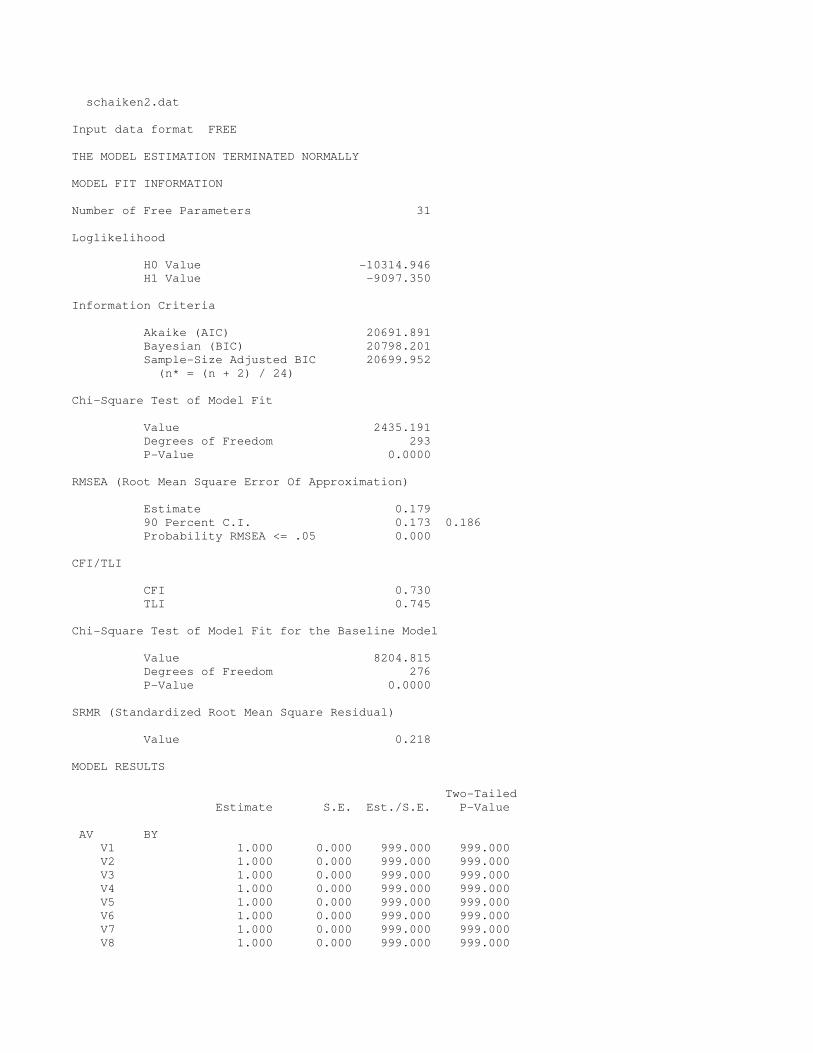
schaiken2.dat
Input data format FREE
THE MODEL ESTIMATION TERMINATED NORMALLY
MODEL FIT INFORMATION
Number of Free Parameters 31
Loglikelihood
H0 Value -10314.946
H1 Value -9097.350
Information Criteria
Akaike (AIC) 20691.891
Bayesian (BIC) 20798.201
Sample-Size Adjusted BIC 20699.952
(n* = (n + 2) / 24)
Chi-Square Test of Model Fit
Value 2435.191
Degrees of Freedom 293
P-Value 0.0000
RMSEA (Root Mean Square Error Of Approximation)
Estimate 0.179
90 Percent C.I. 0.173 0.186
Probability RMSEA <= .05 0.000
CFI/TLI
CFI 0.730
TLI 0.745
Chi-Square Test of Model Fit for the Baseline Model
Value 8204.815
Degrees of Freedom 276
P-Value 0.0000
SRMR (Standardized Root Mean Square Residual)
Value 0.218
MODEL RESULTS
Two-Tailed
Estimate S.E. Est./S.E. P-Value
AV BY
V1 1.000 0.000 999.000 999.000
V2 1.000 0.000 999.000 999.000
V3 1.000 0.000 999.000 999.000
V4 1.000 0.000 999.000 999.000
V5 1.000 0.000 999.000 999.000
V6 1.000 0.000 999.000 999.000
V7 1.000 0.000 999.000 999.000
V8 1.000 0.000 999.000 999.000

V9 1.000 0.000 999.000 999.000
V10 1.000 0.000 999.000 999.000
V11 1.000 0.000 999.000 999.000
V12 1.000 0.000 999.000 999.000
BV BY
V1 -11.004 0.001 ********* 0.000
V2 -5.352 0.105 -50.919 0.000
V3 -2.603 0.102 -25.510 0.000
V4 -1.266 0.074 -17.018 0.000
V5 -0.616 0.048 -12.768 0.000
V6 -0.300 0.029 -10.216 0.000
V7 -0.146 0.017 -8.515 0.000
V8 -0.071 0.010 -7.299 0.000
V9 -0.034 0.005 -6.387 0.000
V10 -0.017 0.003 -5.678 0.000
V11 -0.008 0.002 -5.110 0.000
V12 -0.004 0.001 -4.646 0.000
CV BY
V1 -0.064 0.011 -5.731 0.000
V2 -7.906 0.161 -49.135 0.000
V3 -7.676 0.009 -822.989 0.000
V4 -5.596 0.102 -54.932 0.000
V5 -3.628 0.137 -26.529 0.000
V6 -2.206 0.126 -17.478 0.000
V7 -1.287 0.099 -13.030 0.000
V8 -0.730 0.070 -10.386 0.000
V9 -0.406 0.047 -8.633 0.000
V10 -0.222 0.030 -7.386 0.000
V11 -0.120 0.019 -6.454 0.000
V12 -0.064 0.011 -5.731 0.000
AQ BY
Q1 1.000 0.000 999.000 999.000
Q2 1.000 0.000 999.000 999.000
Q3 1.000 0.000 999.000 999.000
Q4 1.000 0.000 999.000 999.000
Q5 1.000 0.000 999.000 999.000
Q6 1.000 0.000 999.000 999.000
Q7 1.000 0.000 999.000 999.000
Q8 1.000 0.000 999.000 999.000
Q9 1.000 0.000 999.000 999.000
Q10 1.000 0.000 999.000 999.000
Q11 1.000 0.000 999.000 999.000
Q12 1.000 0.000 999.000 999.000
BQ BY
Q1 -11.005 0.001 -8371.135 0.000
Q2 -5.476 0.129 -42.427 0.000
Q3 -2.725 0.128 -21.267 0.000
Q4 -1.356 0.096 -14.190 0.000
Q5 -0.675 0.063 -10.647 0.000
Q6 -0.336 0.039 -8.520 0.000
Q7 -0.167 0.024 -7.101 0.000
Q8 -0.083 0.014 -6.087 0.000
Q9 -0.041 0.008 -5.327 0.000
Q10 -0.021 0.004 -4.735 0.000
Q11 -0.010 0.002 -4.262 0.000
Q12 -0.005 0.001 -3.875 0.000
CQ BY
Q1 -0.079 0.016 -4.809 0.000

Q2 -7.717 0.196 -39.405 0.000
Q3 -7.661 0.020 -387.668 0.000
Q4 -5.713 0.118 -48.419 0.000
Q5 -3.788 0.167 -22.730 0.000
Q6 -2.356 0.159 -14.841 0.000
Q7 -1.406 0.128 -11.015 0.000
Q8 -0.816 0.093 -8.756 0.000
Q9 -0.464 0.064 -7.266 0.000
Q10 -0.260 0.042 -6.209 0.000
Q11 -0.144 0.026 -5.420 0.000
Q12 -0.079 0.016 -4.809 0.000
AV WITH !COVARIANCES OF VERBAL (V) AND
BV -0.193 0.084 -2.303 0.021 !QUANTITATIVE (Q) RANDOM
CV -0.131 0.051 -2.592 0.010 !COEFFICIENTS
AQ 1.664 0.235 7.097 0.000 !
BQ -0.035 0.046 -0.765 0.444 !
CQ -0.037 0.025 -1.494 0.135 !
!
BV WITH !
CV 0.025 0.030 0.834 0.404 !
AQ -0.597 0.126 -4.718 0.000 !
BQ 0.122 0.028 4.403 0.000 !
CQ -0.021 0.014 -1.434 0.152 !
!
AQ WITH !
BQ -0.293 0.068 -4.288 0.000 !
CQ -0.064 0.036 -1.780 0.075 !
!
BQ WITH !
CQ -0.031 0.008 -3.696 0.000 !
!
CV WITH !
AQ -0.183 0.071 -2.558 0.011 !
BQ 0.015 0.016 0.966 0.334 !
CQ 0.016 0.008 2.008 0.045 !
V1 WITH !AUTOREGRESSIVE RESIDUAL
V2 0.544 0.092 5.905 0.000 !COVARIANCE STRUCTURE FOR
V3 0.150 0.045 3.337 0.001 !VERBAL REPEATED MEASURES
V4 0.041 0.018 2.321 0.020 !
V5 0.011 0.006 1.779 0.075 !
V6 0.003 0.002 1.442 0.149 !
V7 0.001 0.001 1.212 0.226 !
V8 0.000 0.000 1.045 0.296 !
V9 0.000 0.000 0.919 0.358 !
V10 0.000 0.000 0.820 0.412 !
V11 0.000 0.000 0.740 0.459 !
V12 0.000 0.000 0.674 0.500 !
!
V2 WITH !
V3 0.544 0.092 5.905 0.000 !
V4 0.150 0.045 3.337 0.001 !
V5 0.041 0.018 2.321 0.020 !
V6 0.011 0.006 1.779 0.075 !
V7 0.003 0.002 1.442 0.149 !
V8 0.001 0.001 1.212 0.226 !
V9 0.000 0.000 1.045 0.296 !
V10 0.000 0.000 0.919 0.358 !
V11 0.000 0.000 0.820 0.412 !
V12 0.000 0.000 0.740 0.459 !
!
V3 WITH !
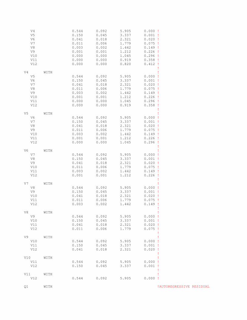
V4 0.544 0.092 5.905 0.000 !
V5 0.150 0.045 3.337 0.001 !
V6 0.041 0.018 2.321 0.020 !
V7 0.011 0.006 1.779 0.075 !
V8 0.003 0.002 1.442 0.149 !
V9 0.001 0.001 1.212 0.226 !
V10 0.000 0.000 1.045 0.296 !
V11 0.000 0.000 0.919 0.358 !
V12 0.000 0.000 0.820 0.412 !
!
V4 WITH !
V5 0.544 0.092 5.905 0.000 !
V6 0.150 0.045 3.337 0.001 !
V7 0.041 0.018 2.321 0.020 !
V8 0.011 0.006 1.779 0.075 !
V9 0.003 0.002 1.442 0.149 !
V10 0.001 0.001 1.212 0.226 !
V11 0.000 0.000 1.045 0.296 !
V12 0.000 0.000 0.919 0.358 !
!
V5 WITH !
V6 0.544 0.092 5.905 0.000 !
V7 0.150 0.045 3.337 0.001 !
V8 0.041 0.018 2.321 0.020 !
V9 0.011 0.006 1.779 0.075 !
V10 0.003 0.002 1.442 0.149 !
V11 0.001 0.001 1.212 0.226 !
V12 0.000 0.000 1.045 0.296 !
!
V6 WITH !
V7 0.544 0.092 5.905 0.000 !
V8 0.150 0.045 3.337 0.001 !
V9 0.041 0.018 2.321 0.020 !
V10 0.011 0.006 1.779 0.075 !
V11 0.003 0.002 1.442 0.149 !
V12 0.001 0.001 1.212 0.226 !
!
V7 WITH !
V8 0.544 0.092 5.905 0.000 !
V9 0.150 0.045 3.337 0.001 !
V10 0.041 0.018 2.321 0.020 !
V11 0.011 0.006 1.779 0.075 !
V12 0.003 0.002 1.442 0.149 !
!
V8 WITH !
V9 0.544 0.092 5.905 0.000 !
V10 0.150 0.045 3.337 0.001 !
V11 0.041 0.018 2.321 0.020 !
V12 0.011 0.006 1.779 0.075 !
!
V9 WITH !
V10 0.544 0.092 5.905 0.000 !
V11 0.150 0.045 3.337 0.001 !
V12 0.041 0.018 2.321 0.020 !
!
V10 WITH !
V11 0.544 0.092 5.905 0.000 !
V12 0.150 0.045 3.337 0.001 !
!
V11 WITH !
V12 0.544 0.092 5.905 0.000 !
Q1 WITH !AUTOREGRESSIVE RESIDUAL

Q2 0.345 0.053 6.528 0.000 !COVARIANCE STRUCTURE FOR
Q3 0.107 0.028 3.787 0.000 !QUANTITATIVE REPEATED MEASURES
Q4 0.033 0.012 2.662 0.008 !
Q5 0.010 0.005 2.051 0.040 !
Q6 0.003 0.002 1.668 0.095 !
Q7 0.001 0.001 1.405 0.160 !
Q8 0.000 0.000 1.214 0.225 !
Q9 0.000 0.000 1.068 0.285 !
Q10 0.000 0.000 0.954 0.340 !
Q11 0.000 0.000 0.862 0.389 !
Q12 0.000 0.000 0.786 0.432 !
!
Q2 WITH !
Q3 0.345 0.053 6.528 0.000 !
Q4 0.107 0.028 3.787 0.000 !
Q5 0.033 0.012 2.662 0.008 !
Q6 0.010 0.005 2.051 0.040 !
Q7 0.003 0.002 1.668 0.095 !
Q8 0.001 0.001 1.405 0.160 !
Q9 0.000 0.000 1.214 0.225 !
Q10 0.000 0.000 1.068 0.285 !
Q11 0.000 0.000 0.954 0.340 !
Q12 0.000 0.000 0.862 0.389 !
!
Q3 WITH !
Q4 0.345 0.053 6.528 0.000 !
Q5 0.107 0.028 3.787 0.000 !
Q6 0.033 0.012 2.662 0.008 !
Q7 0.010 0.005 2.051 0.040 !
Q8 0.003 0.002 1.668 0.095 !
Q9 0.001 0.001 1.405 0.160 !
Q10 0.000 0.000 1.214 0.225 !
Q11 0.000 0.000 1.068 0.285 !
Q12 0.000 0.000 0.954 0.340 !
!
Q4 WITH !
Q5 0.345 0.053 6.528 0.000 !
Q6 0.107 0.028 3.787 0.000 !
Q7 0.033 0.012 2.662 0.008 !
Q8 0.010 0.005 2.051 0.040 !
Q9 0.003 0.002 1.668 0.095 !
Q10 0.001 0.001 1.405 0.160 !
Q11 0.000 0.000 1.214 0.225 !
Q12 0.000 0.000 1.068 0.285 !
!
Q5 WITH !
Q6 0.345 0.053 6.528 0.000 !
Q7 0.107 0.028 3.787 0.000 !
Q8 0.033 0.012 2.662 0.008 !
Q9 0.010 0.005 2.051 0.040 !
Q10 0.003 0.002 1.668 0.095 !
Q11 0.001 0.001 1.405 0.160 !
Q12 0.000 0.000 1.214 0.225 !
!
Q6 WITH !
Q7 0.345 0.053 6.528 0.000 !
Q8 0.107 0.028 3.787 0.000 !
Q9 0.033 0.012 2.662 0.008 !
Q10 0.010 0.005 2.051 0.040 !
Q11 0.003 0.002 1.668 0.095 !
Q12 0.001 0.001 1.405 0.160 !
!
Q7 WITH !

Q8 0.345 0.053 6.528 0.000 !
Q9 0.107 0.028 3.787 0.000 !
Q10 0.033 0.012 2.662 0.008 !
Q11 0.010 0.005 2.051 0.040 !
Q12 0.003 0.002 1.668 0.095 !
!
Q8 WITH !
Q9 0.345 0.053 6.528 0.000 !
Q10 0.107 0.028 3.787 0.000 !
Q11 0.033 0.012 2.662 0.008 !
Q12 0.010 0.005 2.051 0.040 !
!
Q9 WITH !
Q10 0.345 0.053 6.528 0.000 !
Q11 0.107 0.028 3.787 0.000 !
Q12 0.033 0.012 2.662 0.008 !
!
Q10 WITH !
Q11 0.345 0.053 6.528 0.000 !
Q12 0.107 0.028 3.787 0.000 !
!
Q11 WITH !
Q12 0.345 0.053 6.528 0.000 !
Means
AV 0.000 0.000 999.000 999.000 !FACTOR MEANS FIXED = 0
BV 0.000 0.000 999.000 999.000 !
CV 0.000 0.000 999.000 999.000 !
AQ 0.000 0.000 999.000 999.000 !
BQ 0.000 0.000 999.000 999.000 !
CQ 0.000 0.000 999.000 999.000 !
Intercepts
V1 21.278 0.661 32.192 0.000
V2 13.865 0.374 37.074 0.000
V3 10.260 0.238 43.076 0.000
V4 8.506 0.164 51.793 0.000
V5 7.653 0.126 60.759 0.000
V6 7.238 0.109 66.405 0.000
V7 7.036 0.103 68.566 0.000
V8 6.938 0.101 69.035 0.000
V9 6.890 0.100 68.996 0.000
V10 6.867 0.100 68.879 0.000
V11 6.856 0.100 68.788 0.000
V12 6.850 0.100 68.732 0.000
Q1 16.492 0.404 40.779 0.000
Q2 12.541 0.261 47.963 0.000
Q3 10.576 0.202 52.297 0.000
Q4 9.597 0.171 56.084 0.000
Q5 9.111 0.155 58.658 0.000
Q6 8.868 0.148 59.868 0.000
Q7 8.748 0.145 60.270 0.000
Q8 8.688 0.144 60.347 0.000
Q9 8.658 0.144 60.330 0.000
Q10 8.643 0.143 60.299 0.000
Q11 8.636 0.143 60.275 0.000
Q12 8.632 0.143 60.261 0.000
Variances
AV 1.652 0.207 7.981 0.000 !VARIANCES OF RANDOM
BV 0.712 0.069 10.383 0.000 !COEFFICIENTS
CV 0.216 0.023 9.563 0.000 !
AQ 4.187 0.423 9.908 0.000 !

BQ 0.208 0.021 10.104 0.000 !
CQ 0.046 0.006 7.922 0.000 !
Residual Variances
V1 1.974 0.092 21.355 0.000 !VERBAL RESIDUAL VARIANCE
V2 1.974 0.092 21.355 0.000 !HELD EQUAL OVER TIME
V3 1.974 0.092 21.355 0.000 !
V4 1.974 0.092 21.355 0.000 !
V5 1.974 0.092 21.355 0.000 !
V6 1.974 0.092 21.355 0.000 !
V7 1.974 0.092 21.355 0.000 !
V8 1.974 0.092 21.355 0.000 !
V9 1.974 0.092 21.355 0.000 !
V10 1.974 0.092 21.355 0.000 !
V11 1.974 0.092 21.355 0.000 !
V12 1.974 0.092 21.355 0.000 !
Q1 1.112 0.055 20.403 0.000 !QUANTITATIVE RESIDUAL VARIANCE
Q2 1.112 0.055 20.403 0.000 !HELD EQUAL OVER TIME
Q3 1.112 0.055 20.403 0.000 !
Q4 1.112 0.055 20.403 0.000 !
Q5 1.112 0.055 20.403 0.000 !
Q6 1.112 0.055 20.403 0.000 !
Q7 1.112 0.055 20.403 0.000 !
Q8 1.112 0.055 20.403 0.000 !
Q9 1.112 0.055 20.403 0.000 !
Q10 1.112 0.055 20.403 0.000 !
Q11 1.112 0.055 20.403 0.000 !
Q12 1.112 0.055 20.403 0.000 !
New/Additional Parameters
MAV 6.845 0.100 68.666 0.000 !VERBAL MEAN ASYMPTOTE
MBV -1.312 0.058 -22.498 0.000 !VERBAL MEAN ARC PARAMETER
MCV 1.962 0.026 75.155 0.000 !VERBAL MEAN HALF-LIFE
MAQ 8.629 0.143 60.242 0.000 !QUANT. MEAN ASYMPTOTE
MBQ -0.715 0.031 -23.159 0.000 !QUANT. MEAN ARC PARAMETER
MCQ 1.993 0.033 59.738 0.000 !QUANT. MEAN HALF-LIFE
RHOV 0.276 0.036 7.597 0.000 !AUTOREGRESSIVE PARAMETER (V)
RHOQ 0.310 0.035 8.910 0.000 !AUTOREGRESSIVE PARAMETER (Q)
DIFF -0.031 0.042 -0.749 0.454 !DIFFERENCE IN HALF-LIFES
QUALITY OF NUMERICAL RESULTS
Condition Number for the Information Matrix 0.214E-04
(ratio of smallest to largest eigenvalue)
14. Annotated output: quadratic function fit to Kanfer & Ackerman’s data (traditional)
Mplus VERSION 7.2
MUTHEN & MUTHEN
06/10/2014 11:00 PM
INPUT INSTRUCTIONS
TITLE: Cudeck and du Toit (2002) quadratic curve;
DATA: FILE IS kanfer.dat; !data file in ascii format
TYPE IS COVARIANCE MEANS; !input data are covariances and means
NOBSERVATIONS IS 140; !sample size is 140
VARIABLE: NAMES ARE y1-y9; !all 9 variables
ANALYSIS: ESTIMATOR=ML; !use maximum likelihood estimation
ITERATIONS=5000; !use 5000 iterations
MODEL: y1-y9*9.9(v); [y1-y9@0]; !residual covariances constrained equal, intercepts = 0
[a0*16 ay*39](ma0 may); [ax@0]; !intercept and maximum means estimated, maximizer = 0

a0*123; ax*18; ay*53; !random coefficient variances
a0 WITH ax*-.8 ay*35; ax WITH ay*8.9; !random coefficient covariances
a0 BY y1-y9*(a01-a09); ax BY y1-y9*(ax1-ax9); ay BY y1-y9*(ay1-ay9); !loadings
MODEL CONSTRAINT: NEW(max*8.8); !define maximizer mean
!loadings on maximum, intercept, and maximizer factors, constrained to
!d(y)/d(may), d(y)/d(ma0), and d(y)/d(max)
ay1=1-((0/max)-1)^2; a01=((0/max)-1)^2; ax1=2*(may-ma0)*(0-max)*0/max^3;
ay2=1-((1/max)-1)^2; a02=((1/max)-1)^2; ax2=2*(may-ma0)*(1-max)*1/max^3;
ay3=1-((2/max)-1)^2; a03=((2/max)-1)^2; ax3=2*(may-ma0)*(2-max)*2/max^3;
ay4=1-((3/max)-1)^2; a04=((3/max)-1)^2; ax4=2*(may-ma0)*(3-max)*3/max^3;
ay5=1-((4/max)-1)^2; a05=((4/max)-1)^2; ax5=2*(may-ma0)*(4-max)*4/max^3;
ay6=1-((5/max)-1)^2; a06=((5/max)-1)^2; ax6=2*(may-ma0)*(5-max)*5/max^3;
ay7=1-((6/max)-1)^2; a07=((6/max)-1)^2; ax7=2*(may-ma0)*(6-max)*6/max^3;
ay8=1-((7/max)-1)^2; a08=((7/max)-1)^2; ax8=2*(may-ma0)*(7-max)*7/max^3;
ay9=1-((8/max)-1)^2; a09=((8/max)-1)^2; ax9=2*(may-ma0)*(8-max)*8/max^3;
OUTPUT: TECH1 TECH4;
INPUT READING TERMINATED NORMALLY
Cudeck and du Toit (2002) quadratic curve;
SUMMARY OF ANALYSIS
Number of groups 1
Number of observations 140
Number of dependent variables 9
Number of independent variables 0
Number of continuous latent variables 3
Observed dependent variables
Continuous
Y1 Y2 Y3 Y4 Y5 Y6
Y7 Y8 Y9
Continuous latent variables
A0 AX AY
Estimator ML
Information matrix EXPECTED
Maximum number of iterations 5000
Convergence criterion 0.500D-04
Maximum number of steepest descent iterations 20
Input data file(s)
kanfer.dat
Input data format FREE
THE MODEL ESTIMATION TERMINATED NORMALLY
MODEL FIT INFORMATION
Number of Free Parameters 10
Loglikelihood
H0 Value -3743.236
H1 Value -3645.210

Information Criteria
Akaike (AIC) 7506.473
Bayesian (BIC) 7535.889
Sample-Size Adjusted BIC 7504.251
(n* = (n + 2) / 24)
Chi-Square Test of Model Fit
Value 196.054
Degrees of Freedom 44
P-Value 0.0000
RMSEA (Root Mean Square Error Of Approximation)
Estimate 0.157
90 Percent C.I. 0.135 0.180
Probability RMSEA <= .05 0.000
CFI/TLI
CFI 0.909
TLI 0.925
Chi-Square Test of Model Fit for the Baseline Model
Value 1702.962
Degrees of Freedom 36
P-Value 0.0000
SRMR (Standardized Root Mean Square Residual)
Value 0.076
MODEL RESULTS
Two-Tailed
Estimate S.E. Est./S.E. P-Value
A0 BY
Y1 1.000 0.000 999.000 999.000
Y2 0.760 0.012 64.221 0.000
Y3 0.552 0.020 27.380 0.000
Y4 0.378 0.025 15.099 0.000
Y5 0.237 0.026 8.959 0.000
Y6 0.128 0.024 5.275 0.000
Y7 0.053 0.019 2.819 0.005
Y8 0.010 0.010 1.064 0.287
Y9 0.001 0.003 0.252 0.801
AX BY
Y1 0.000 0.000 999.000 999.000
Y2 -0.519 0.046 11.153 0.000
Y3 -0.884 0.071 12.430 0.000
Y4 -1.097 0.075 14.701 0.000
Y5 -1.157 0.060 19.389 0.000
Y6 -1.065 0.044 24.352 0.000
Y7 -0.819 0.081 10.172 0.000
Y8 -0.421 0.162 2.603 0.009
Y9 0.130 0.270 -0.482 0.630
AY BY

Y1 0.000 0.000 999.000 999.000
Y2 0.240 0.012 20.318 0.000
Y3 0.448 0.020 22.194 0.000
Y4 0.622 0.025 24.853 0.000
Y5 0.763 0.026 28.917 0.000
Y6 0.872 0.024 35.897 0.000
Y7 0.947 0.019 50.687 0.000
Y8 0.990 0.010 103.048 0.000
Y9 0.999 0.003 336.999 0.000
A0 WITH !COVARIANCES OF RANDOM
AX -8.248 4.168 -1.979 0.048 !COEFFICIENTS
AY 34.623 7.489 4.623 0.000 !
!
AX WITH !
AY 8.864 6.611 1.341 0.180 !
Means
A0 20.732 0.846 24.510 0.000 !MEAN INTERCEPT (ESTIMATED)
AX 0.000 0.000 999.000 999.000 !MEAN MAXIMIZER (FIXED = 0)
AY 38.772 0.655 59.185 0.000 !MEAN MAXIMUM (ESTIMATED)
Intercepts
Y1 0.000 0.000 999.000 999.000 !REPEATED MEASURE INTERCEPTS
Y2 0.000 0.000 999.000 999.000 !ALL FIXED = 0
Y3 0.000 0.000 999.000 999.000 !
Y4 0.000 0.000 999.000 999.000 !
Y5 0.000 0.000 999.000 999.000 !
Y6 0.000 0.000 999.000 999.000 !
Y7 0.000 0.000 999.000 999.000 !
Y8 0.000 0.000 999.000 999.000 !
Y9 0.000 0.000 999.000 999.000 !
Variances
A0 93.610 11.976 7.816 0.000 !VARIANCE OF INTERCEPT FACTOR
AX 18.019 6.969 2.585 0.010 !VARIANCE OF MAXIMIZER FACTOR
AY 54.708 8.395 6.517 0.000 !VARIANCE OF MAXIMUM FACTOR
Residual Variances
Y1 9.921 0.484 20.494 0.000 !RESIDUAL VARIANCE HELD EQUAL
Y2 9.921 0.484 20.494 0.000 !OVER TIME
Y3 9.921 0.484 20.494 0.000 !
Y4 9.921 0.484 20.494 0.000 !
Y5 9.921 0.484 20.494 0.000 !
Y6 9.921 0.484 20.494 0.000 !
Y7 9.921 0.484 20.494 0.000 !
Y8 9.921 0.484 20.494 0.000 !
Y9 9.921 0.484 20.494 0.000 !
New/Additional Parameters
MAX 7.787 0.412 18.924 0.000 !MEAN MAXIMIZER
QUALITY OF NUMERICAL RESULTS
Condition Number for the Information Matrix 0.200E-03
(ratio of smallest to largest eigenvalue)
15. Annotated output: quadratic function fit to Kanfer & Ackerman’s data (modified)
Mplus VERSION 7.2
MUTHEN & MUTHEN

06/10/2014 11:00 PM
INPUT INSTRUCTIONS
TITLE: Cudeck and du Toit (2002) quadratic curve;
DATA: FILE IS kanfer.dat; !data file in ascii format
TYPE IS COVARIANCE MEANS; !input data are covariances and means
NOBSERVATIONS IS 140; !sample size is 140
VARIABLE: NAMES ARE y1-y9; !all 9 variables
ANALYSIS: ESTIMATOR=ML; !use maximum likelihood estimation
ITERATIONS=5000; !use 5000 iterations
MODEL: [y1-y9*](my1-my9); !intercepts constrained equal to target function
y1-y9*9.9(v); !residual covariances constrained equal
[a0@0 ax@0 ay@0]; !factor means constrained to zero
a0*123; ax*18; ay*53; !random coefficient variances
a0 WITH ax*-.8 ay*35; ax WITH ay*8.9; !random coefficient covariances
a0 BY y1-y9*(a01-a09); ax BY y1-y9*(ax1-ax9); ay BY y1-y9*(ay1-ay9); !loadings
MODEL CONSTRAINT:
NEW(ma0*16 max*8.8 may*39); !define mean intercept, maximizer, and maximum
!intercepts constrained equal to target function
my1=may-(may-ma0)*((0/max)-1)^2;
my2=may-(may-ma0)*((1/max)-1)^2;
my3=may-(may-ma0)*((2/max)-1)^2;
my4=may-(may-ma0)*((3/max)-1)^2;
my5=may-(may-ma0)*((4/max)-1)^2;
my6=may-(may-ma0)*((5/max)-1)^2;
my7=may-(may-ma0)*((6/max)-1)^2;
my8=may-(may-ma0)*((7/max)-1)^2;
my9=may-(may-ma0)*((8/max)-1)^2;
!loadings on maximum, intercept, and maximizer factors, constrained to
!d(y)/d(may), d(y)/d(ma0), and d(y)/d(max)
ay1=1-((0/max)-1)^2; a01=((0/max)-1)^2; ax1=2*(may-ma0)*(0-max)*0/max^3;
ay2=1-((1/max)-1)^2; a02=((1/max)-1)^2; ax2=2*(may-ma0)*(1-max)*1/max^3;
ay3=1-((2/max)-1)^2; a03=((2/max)-1)^2; ax3=2*(may-ma0)*(2-max)*2/max^3;
ay4=1-((3/max)-1)^2; a04=((3/max)-1)^2; ax4=2*(may-ma0)*(3-max)*3/max^3;
ay5=1-((4/max)-1)^2; a05=((4/max)-1)^2; ax5=2*(may-ma0)*(4-max)*4/max^3;
ay6=1-((5/max)-1)^2; a06=((5/max)-1)^2; ax6=2*(may-ma0)*(5-max)*5/max^3;
ay7=1-((6/max)-1)^2; a07=((6/max)-1)^2; ax7=2*(may-ma0)*(6-max)*6/max^3;
ay8=1-((7/max)-1)^2; a08=((7/max)-1)^2; ax8=2*(may-ma0)*(7-max)*7/max^3;
ay9=1-((8/max)-1)^2; a09=((8/max)-1)^2; ax9=2*(may-ma0)*(8-max)*8/max^3;
OUTPUT: TECH1 TECH4;
INPUT READING TERMINATED NORMALLY
Cudeck and du Toit (2002) quadratic curve;
SUMMARY OF ANALYSIS
Number of groups 1
Number of observations 140
Number of dependent variables 9
Number of independent variables 0
Number of continuous latent variables 3
Observed dependent variables
Continuous
Y1 Y2 Y3 Y4 Y5 Y6

Y7 Y8 Y9
Continuous latent variables
A0 AX AY
Estimator ML
Information matrix EXPECTED
Maximum number of iterations 5000
Convergence criterion 0.500D-04
Maximum number of steepest descent iterations 20
Input data file(s)
kanfer.dat
Input data format FREE
THE MODEL ESTIMATION TERMINATED NORMALLY
MODEL FIT INFORMATION
Number of Free Parameters 10
Loglikelihood
H0 Value -3743.236
H1 Value -3645.210
Information Criteria
Akaike (AIC) 7506.473
Bayesian (BIC) 7535.889
Sample-Size Adjusted BIC 7504.251
(n* = (n + 2) / 24)
Chi-Square Test of Model Fit
Value 196.054
Degrees of Freedom 44
P-Value 0.0000
RMSEA (Root Mean Square Error Of Approximation)
Estimate 0.157
90 Percent C.I. 0.135 0.180
Probability RMSEA <= .05 0.000
CFI/TLI
CFI 0.909
TLI 0.925
Chi-Square Test of Model Fit for the Baseline Model
Value 1702.962
Degrees of Freedom 36
P-Value 0.0000
SRMR (Standardized Root Mean Square Residual)
Value 0.076
MODEL RESULTS

Two-Tailed
Estimate S.E. Est./S.E. P-Value
A0 BY
Y1 1.000 0.000 999.000 999.000
Y2 0.760 0.012 64.222 0.000
Y3 0.552 0.020 27.380 0.000
Y4 0.378 0.025 15.099 0.000
Y5 0.237 0.026 8.959 0.000
Y6 0.128 0.024 5.275 0.000
Y7 0.053 0.019 2.819 0.005
Y8 0.010 0.010 1.064 0.287
Y9 0.001 0.003 0.252 0.801
AX BY
Y1 0.000 0.000 999.000 999.000
Y2 -0.519 0.046 -11.154 0.000
Y3 -0.884 0.071 -12.430 0.000
Y4 -1.097 0.075 -14.701 0.000
Y5 -1.157 0.060 -19.389 0.000
Y6 -1.065 0.044 -24.352 0.000
Y7 -0.819 0.081 -10.172 0.000
Y8 -0.421 0.162 -2.603 0.009
Y9 0.130 0.270 0.482 0.630
AY BY
Y1 0.000 0.000 999.000 999.000
Y2 0.240 0.012 20.318 0.000
Y3 0.448 0.020 22.194 0.000
Y4 0.622 0.025 24.854 0.000
Y5 0.763 0.026 28.918 0.000
Y6 0.872 0.024 35.897 0.000
Y7 0.947 0.019 50.688 0.000
Y8 0.990 0.010 103.050 0.000
Y9 0.999 0.003 336.998 0.000
A0 WITH !COVARIANCES OF RANDOM
AX -8.248 4.168 -1.979 0.048 !COEFFICIENTS
AY 34.624 7.489 4.623 0.000 !
!
AX WITH !
AY 8.864 6.610 1.341 0.180 !
Means
A0 0.000 0.000 999.000 999.000 !FACTOR MEANS FIXED = 0
AX 0.000 0.000 999.000 999.000 !
AY 0.000 0.000 999.000 999.000 !
Intercepts
Y1 20.732 0.846 24.510 0.000 !REPEATED MEASURE INTERCEPTS
Y2 25.067 0.764 32.809 0.000 !FIXED EQUAL TO THE TARGET
Y3 28.808 0.726 39.688 0.000 !FUNCTION
Y4 31.954 0.705 45.333 0.000 !
Y5 34.505 0.682 50.579 0.000 !
Y6 36.461 0.651 55.983 0.000 !
Y7 37.821 0.620 60.982 0.000 !
Y8 38.587 0.615 62.745 0.000 !
Y9 38.758 0.675 57.397 0.000 !
Variances
A0 93.610 11.976 7.816 0.000 !VARIANCE OF INTERCEPT FACTOR
AX 18.019 6.969 2.585 0.010 !VARIANCE OF MAXIMIZER FACTOR
AY 54.708 8.395 6.517 0.000 !VARIANCE OF MAXIMUM FACTOR

Residual Variances
Y1 9.921 0.484 20.494 0.000 !RESIDUAL VARIANCE HELD EQUAL
Y2 9.921 0.484 20.494 0.000 !OVER TIME
Y3 9.921 0.484 20.494 0.000 !
Y4 9.921 0.484 20.494 0.000 !
Y5 9.921 0.484 20.494 0.000 !
Y6 9.921 0.484 20.494 0.000 !
Y7 9.921 0.484 20.494 0.000 !
Y8 9.921 0.484 20.494 0.000 !
Y9 9.921 0.484 20.494 0.000 !
New/Additional Parameters
MA0 20.732 0.846 24.510 0.000 !MEAN INTERCEPT
MAX 7.787 0.412 18.924 0.000 !MEAN MAXIMIZER
MAY 38.772 0.655 59.185 0.000 !MEAN MAXIMUM
QUALITY OF NUMERICAL RESULTS
Condition Number for the Information Matrix 0.647E-05
(ratio of smallest to largest eigenvalue)