pratt truss bridge - COMSOL Multiphysics · PRATT TRUSS BRIDGE . Figure . 4 shows the stress...
26
Solved with COMSOL Multiphysics 4.3a ©2012 COMSOL 1 | PRATT TRUSS BRIDGE Pratt Truss Bridge Introduction This example is inspired by a classic bridge type called a Pratt truss bridge. You can identify a Pratt truss by its diagonal members, which (except for the very end ones) all slant down and in toward the center of the span. All the diagonal members are subject to tension forces only, while the shorter vertical members handle the compressive forces. Since the tension removes the buckling risk, this allows for thinner diagonal members resulting in a more economic design. A truss structure supports only tension and compression forces in its members and you would normally model it using bars, but as this model uses 3D beams it also includes bending moments to some extent in a frame structure. In the model, shell elements represent the roadway. Model Definition BASIC DIMENSIONS The length of the bridge is 40 m, and the width of the roadway is 7 m. The main distance between the truss members is 5 m. ANALYSIS TYPES The model includes two different analyses of the bridge: • The goal of the first analysis is to evaluate the stress and deflection fields of the bridge when exposed to a pure gravity load and also when a load corresponding to one or two trucks crosses the bridge. • Finally, an eigenfrequency analysis shows the eigenfrequencies and eigenmodes of the bridge. LOADS AND CONSTRAINTS To prevent rigid body motion of the bridge, it is important to constrain it properly. All translational degrees of freedom are constrained at the left-most horizontal edge. Constraints at the right-most horizontal edge prevent it from moving in the vertical and transversal directions but allow the bridge to expand or contract in the axial
Transcript of pratt truss bridge - COMSOL Multiphysics · PRATT TRUSS BRIDGE . Figure . 4 shows the stress...

Solved with COMSOL Multiphysics 4.3a
© 2 0 1 2 C O
P r a t t T r u s s B r i d g e
Introduction
This example is inspired by a classic bridge type called a Pratt truss bridge. You can identify a Pratt truss by its diagonal members, which (except for the very end ones) all slant down and in toward the center of the span. All the diagonal members are subject to tension forces only, while the shorter vertical members handle the compressive forces. Since the tension removes the buckling risk, this allows for thinner diagonal members resulting in a more economic design.
A truss structure supports only tension and compression forces in its members and you would normally model it using bars, but as this model uses 3D beams it also includes bending moments to some extent in a frame structure. In the model, shell elements represent the roadway.
Model Definition
B A S I C D I M E N S I O N S
The length of the bridge is 40 m, and the width of the roadway is 7 m. The main distance between the truss members is 5 m.
A N A L Y S I S TY P E S
The model includes two different analyses of the bridge:
• The goal of the first analysis is to evaluate the stress and deflection fields of the bridge when exposed to a pure gravity load and also when a load corresponding to one or two trucks crosses the bridge.
• Finally, an eigenfrequency analysis shows the eigenfrequencies and eigenmodes of the bridge.
L O A D S A N D C O N S T R A I N T S
To prevent rigid body motion of the bridge, it is important to constrain it properly. All translational degrees of freedom are constrained at the left-most horizontal edge. Constraints at the right-most horizontal edge prevent it from moving in the vertical and transversal directions but allow the bridge to expand or contract in the axial
M S O L 1 | P R A T T TR U S S B R I D G E
Solved with COMSOL Multiphysics 4.3a
2 | P R A
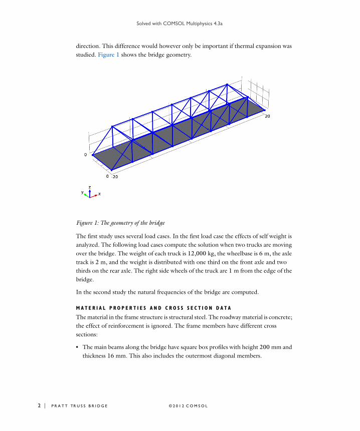
direction. This difference would however only be important if thermal expansion was studied. Figure 1 shows the bridge geometry.
Figure 1: The geometry of the bridge
The first study uses several load cases. In the first load case the effects of self weight is analyzed. The following load cases compute the solution when two trucks are moving over the bridge. The weight of each truck is 12,000 kg, the wheelbase is 6 m, the axle track is 2 m, and the weight is distributed with one third on the front axle and two thirds on the rear axle. The right side wheels of the truck are 1 m from the edge of the bridge.
In the second study the natural frequencies of the bridge are computed.
M A T E R I A L P R O P E R T I E S A N D C R O S S S E C T I O N D A T A
The material in the frame structure is structural steel. The roadway material is concrete; the effect of reinforcement is ignored. The frame members have different cross sections:
• The main beams along the bridge have square box profiles with height 200 mm and thickness 16 mm. This also includes the outermost diagonal members.
T T TR U S S B R I D G E © 2 0 1 2 C O M S O L
Solved with COMSOL Multiphysics 4.3a
© 2 0 1 2 C O
• The diagonal and vertical members have a rectangular box section 200x100 mm, with 12.5 mm thickness. The large dimension is in the transverse direction of the bridge.
• The transverse horizontal members supporting the roadway (floor beams) are standard HEA100 profiles.
• The transverse horizontal members at the top of the truss (struts) are made from solid rectangular sections with dimension 100x25 mm. The large dimension is in the horizontal direction.
Results and Discussion
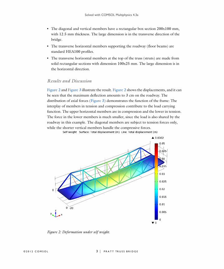
Figure 2 and Figure 3 illustrate the result. Figure 2 shows the displacements, and it can be seen that the maximum deflection amounts to 3 cm on the roadway. The distribution of axial forces (Figure 3) demonstrates the function of the frame: The interplay of members in tension and compression contribute to the load carrying function. The upper horizontal members are in compression and the lower in tension. The force in the lower members is much smaller, since the load is also shared by the roadway in this example. The diagonal members are subject to tension forces only, while the shorter vertical members handle the compressive forces.
Figure 2: Deformation under self weight.
M S O L 3 | P R A T T TR U S S B R I D G E

Solved with COMSOL Multiphysics 4.3a
4 | P R A
Figure 3: The axial forces in the beams. Red is tension and blue is compression.
To study the effects of trucks moving over the bridge several load cases represent the position of the trucks, which are moved 3 m along the bridge for each load case.
T T TR U S S B R I D G E © 2 0 1 2 C O M S O L
Solved with COMSOL Multiphysics 4.3a
© 2 0 1 2 C O
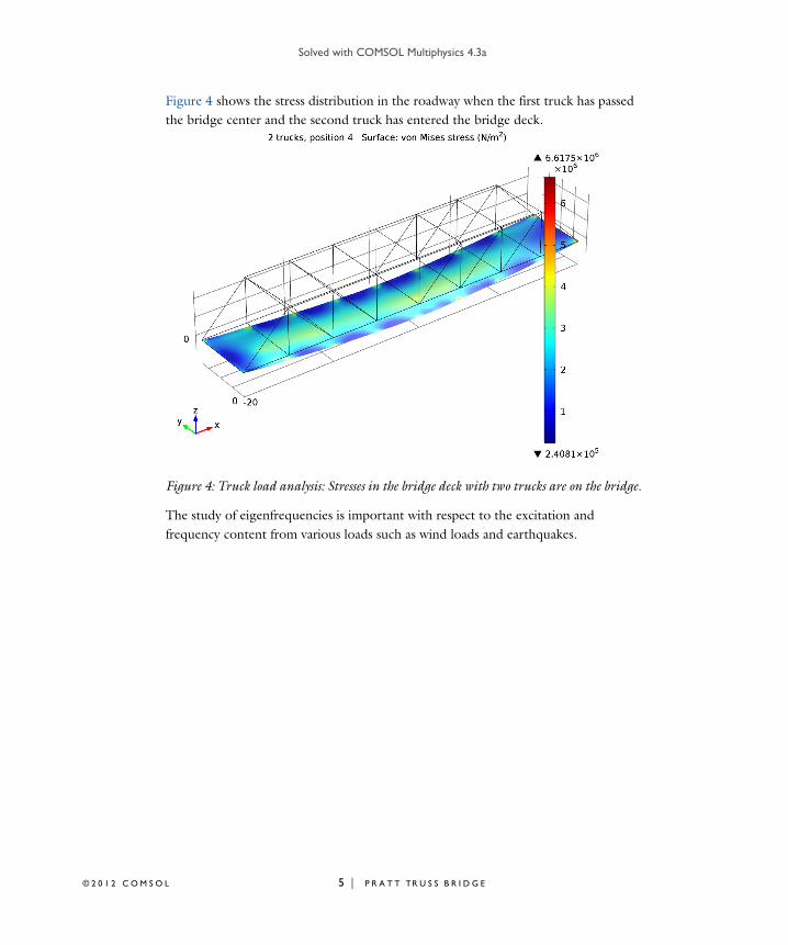
Figure 4 shows the stress distribution in the roadway when the first truck has passed the bridge center and the second truck has entered the bridge deck.
Figure 4: Truck load analysis: Stresses in the bridge deck with two trucks are on the bridge.
The study of eigenfrequencies is important with respect to the excitation and frequency content from various loads such as wind loads and earthquakes.
M S O L 5 | P R A T T TR U S S B R I D G E
Solved with COMSOL Multiphysics 4.3a
6 | P R A
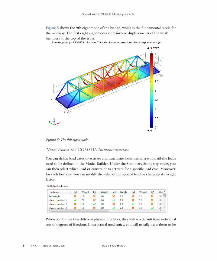
Figure 5 shows the 9th eigenmode of the bridge, which is the fundamental mode for the roadway. The first eight eigenmodes only involve displacements of the weak members at the top of the truss.
Figure 5: The 9th eigenmode.
Notes About the COMSOL Implementation
You can define load cases to activate and deactivate loads within a study. All the loads need to be defined in the Model Builder. Under the Stationary Study step node, you can then select which load or constraint to activate for a specific load case. Moreover for each load case you can modify the value of the applied load by changing its weight factor.
When combining two different physics interfaces, they will as a default have individual sets of degrees of freedom. In structural mechanics, you will usually want them to be
T T TR U S S B R I D G E © 2 0 1 2 C O M S O L
Solved with COMSOL Multiphysics 4.3a
© 2 0 1 2 C O
equal, so you rename the displacements in the second interface to have the same name as in the first interface. In this case, where both beams and shells have rotational degrees of freedom, also these will in general need to treated. The representation of rotation is however different in the Shell and Beam interface, so the simple renaming cannot be used. In the example you can see how the rotations in the beam elements are prescribed to follow those in the shell to which they are connected. In models like this, the results will be virtually the same if the connection of rotations is omitted, as long as the mesh is reasonably fine.
Model Library path: Structural_Mechanics_Module/Civil_Engineering/pratt_truss_bridge
Modeling Instructions
M O D E L W I Z A R D
1 Go to the Model Wizard window.
2 Click Next.
3 In the Add physics tree, select Structural Mechanics>Shell (shell).
4 Click Add Selected.
5 In the Add physics tree, select Structural Mechanics>Beam (beam).
6 Click Add Selected.
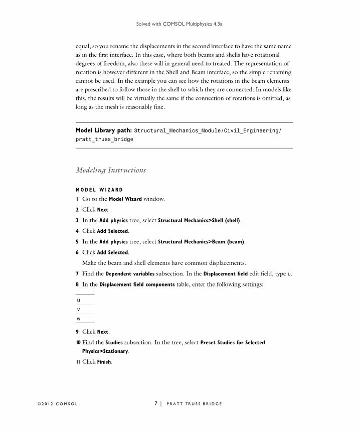
Make the beam and shell elements have common displacements.
7 Find the Dependent variables subsection. In the Displacement field edit field, type u.
8 In the Displacement field components table, enter the following settings:
9 Click Next.
10 Find the Studies subsection. In the tree, select Preset Studies for Selected
Physics>Stationary.
11 Click Finish.
u
v
w
M S O L 7 | P R A T T TR U S S B R I D G E
Solved with COMSOL Multiphysics 4.3a
8 | P R A
G L O B A L D E F I N I T I O N S
Parameters1 In the Model Builder window, right-click Global Definitions and choose Parameters.
2 In the Parameters settings window, locate the Parameters section.
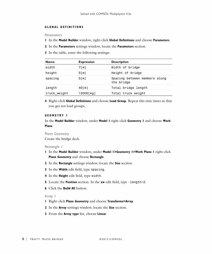
3 In the table, enter the following settings:
4 Right-click Global Definitions and choose Load Group. Repeat this nine times so that you get ten load groups.
G E O M E T R Y 1
In the Model Builder window, under Model 1 right-click Geometry 1 and choose Work
Plane.
Plane GeometryCreate the bridge deck.
Rectangle 11 In the Model Builder window, under Model 1>Geometry 1>Work Plane 1 right-click
Plane Geometry and choose Rectangle.
2 In the Rectangle settings window, locate the Size section.
3 In the Width edit field, type spacing.
4 In the Height edit field, type width.
5 Locate the Position section. In the xw edit field, type -length/2.
6 Click the Build All button.
Array 11 Right-click Plane Geometry and choose Transforms>Array.
2 In the Array settings window, locate the Size section.
3 From the Array type list, choose Linear.
Name Expression Description
width 7[m] Width of bridge
height 5[m] Height of bridge
spacing 5[m] Spacing between members along the bridge
length 40[m] Total bridge length
truck_weight 12000[kg] Total truck weight
T T TR U S S B R I D G E © 2 0 1 2 C O M S O L

Solved with COMSOL Multiphysics 4.3a
© 2 0 1 2 C O
4 Select the object r1 only.
5 In the Size edit field, type length/spacing.
6 Locate the Displacement section. In the xw edit field, type spacing.
7 Click the Build All button.
8 Click the Zoom Extents button on the Graphics toolbar.
Plane GeometryMake it possible to create beams along the edges.
Convert to Curve 11 Right-click Plane Geometry and choose Conversions>Convert to Curve.
2 In the Convert to Curve settings window, locate the Input section.
3 Select the Keep input objects check box.
4 Click in the Graphics window, press Ctrl+A to highlight all objects, and then right-click to confirm the selection.
5 Click the Build All button.
6 In the Model Builder window, right-click Geometry 1 and choose Build All.
7 Click the Zoom Extents button on the Graphics toolbar.
Start creating the truss.
Work Plane 21 Right-click Geometry 1 and choose Work Plane.
2 In the Work Plane settings window, locate the Work Plane section.
3 From the Plane list, choose xz-plane.
Bézier Polygon 11 In the Model Builder window, under Model 1>Geometry 1>Work Plane 2 right-click
Plane Geometry and choose Bézier Polygon.
2 In the Bézier Polygon settings window, locate the General section.
3 From the Type list, choose Open curve.
4 Locate the Polygon Segments section. Find the Added segments subsection. Click the Add Linear button.
5 Find the Control points subsection. In row 2, set xw to spacing.
6 In row 2, set yw to height.
7 Find the Added segments subsection. Click the Add Linear button.
M S O L 9 | P R A T T TR U S S B R I D G E

Solved with COMSOL Multiphysics 4.3a
10 | P R A
8 Find the Control points subsection. In row 2, set yw to 0.
9 Click the Build All button.
Bézier Polygon 21 Right-click Plane Geometry and choose Bézier Polygon.
2 In the Bézier Polygon settings window, locate the General section.
3 From the Type list, choose Open curve.
4 Locate the Polygon Segments section. Find the Added segments subsection. Click the Add Linear button.
5 Find the Control points subsection. In row 1, set yw to height.
6 In row 2, set xw to spacing.
7 In row 2, set yw to height.
8 Click the Build All button.
Array 11 Right-click Plane Geometry and choose Transforms>Array.
2 In the Array settings window, locate the Size section.
3 From the Array type list, choose Linear.
4 Select the objects b1 and b2 only.
5 In the Size edit field, type length/(2*spacing)-1.
6 Locate the Displacement section. In the xw edit field, type spacing.
7 Click the Build All button.
Bézier Polygon 31 Right-click Plane Geometry and choose Bézier Polygon.
2 In the Bézier Polygon settings window, locate the General section.
3 From the Type list, choose Open curve.
4 Locate the Polygon Segments section. Find the Added segments subsection. Click the Add Linear button.
5 Find the Control points subsection. In row 1, set xw to length/2-spacing.
6 In row 1, set yw to height.
7 In row 2, set xw to length/2.
8 Click the Build All button.
T T TR U S S B R I D G E © 2 0 1 2 C O M S O L

Solved with COMSOL Multiphysics 4.3a
© 2 0 1 2 C O
Mirror 11 Right-click Plane Geometry and choose Transforms>Mirror.
2 Click in the Graphics window, press Ctrl+A to highlight all objects, and then right-click to confirm the selection.
3 In the Mirror settings window, locate the Input section.
4 Select the Keep input objects check box.
5 Click the Build All button.
6 Click the Zoom Extents button on the Graphics toolbar.
Bézier Polygon 41 Right-click Plane Geometry and choose Bézier Polygon.
2 In the Bézier Polygon settings window, locate the General section.
3 From the Type list, choose Open curve.
4 Locate the Polygon Segments section. Find the Added segments subsection. Click the Add Linear button.
5 Find the Control points subsection. In row 2, set yw to height.
6 Click the Build All button.
7 In the Model Builder window, right-click Geometry 1 and choose Build All.
Copy 11 Right-click Geometry 1 and choose Transforms>Copy.
2 In the Copy settings window, locate the Displacement section.
3 In the y edit field, type width.
4 Select all edges that are not part of the bridge deck. (wp2.arr1(1,2), wp2.arr1(3,1), wp2.arr1(2,1), wp2.arr1(1,1), wp2.mir1(1), wp2.b3, wp2.arr1(3,2), wp2.arr1(2,2), wp2.mir1(6), wp2.mir1(7), wp2.b4, wp2.mir1(2), wp2.mir1(3), wp2.mir1(4), and wp2.mir1(5)).
5 Click the Build All button.
Bézier Polygon 11 Right-click Geometry 1 and choose More Primitives>Bézier Polygon.
2 In the Bézier Polygon settings window, locate the Polygon Segments section.
3 Find the Added segments subsection. Click the Add Linear button.
4 Find the Control points subsection. In row 1, set x to -length/2+spacing.
5 In row 1, set z to height.
M S O L 11 | P R A T T TR U S S B R I D G E

Solved with COMSOL Multiphysics 4.3a
12 | P R A
6 In row 2, set x to -length/2+spacing.
7 In row 2, set y to width.
8 In row 2, set z to height.
9 Click the Build All button.
Array 11 Right-click Geometry 1 and choose Transforms>Array.
2 Select the object b1 only.
3 In the Array settings window, locate the Size section.
4 From the Array type list, choose Linear.
5 Locate the Displacement section. In the x edit field, type spacing.
6 Locate the Size section. In the Size edit field, type length/spacing-1.
Create points in the positions where the loads from the truck wheels are to be applied.
Point 11 Right-click Geometry 1 and choose More Primitives>Point.
2 In the Point settings window, locate the Point section.
3 In the x edit field, type -19.
4 In the y edit field, type 1.
Array 21 Right-click Geometry 1 and choose Transforms>Array.
2 Select the object pt1 only.
3 In the Array settings window, locate the Size section.
4 In the x size edit field, type 10.
5 In the y size edit field, type 2.
6 Locate the Displacement section. In the x edit field, type 3.
7 In the y edit field, type 2.
8 Click the Build All button.
D E F I N I T I O N S
Create groups for the different beam sections.
Box 11 In the Model Builder window, under Model 1 right-click Definitions and choose
Selections>Box.
T T TR U S S B R I D G E © 2 0 1 2 C O M S O L

Solved with COMSOL Multiphysics 4.3a
© 2 0 1 2 C O
2 In the Box settings window, locate the Geometric Entity Level section.
3 From the Level list, choose Edge.
4 Locate the Box Limits section. In the x minimum edit field, type -(length/2+1).
5 In the x maximum edit field, type length/2+1.
6 In the y minimum edit field, type 1.
7 In the y maximum edit field, type width-1.
8 In the z minimum edit field, type -1.
9 In the z maximum edit field, type 1.
10 Right-click Model 1>Definitions>Box 1 and choose Rename.
11 Go to the Rename Box dialog box and type BeamsTransvBelow in the New name edit field.
12 Click OK.
Box 21 Right-click Definitions and choose Selections>Box.
2 In the Box settings window, locate the Geometric Entity Level section.
3 From the Level list, choose Edge.
4 Locate the Box Limits section. In the x minimum edit field, type -(length/2+1).
5 In the x maximum edit field, type length/2+1.
6 In the y minimum edit field, type 1.
7 In the y maximum edit field, type width-1.
8 In the z minimum edit field, type height-1.
9 In the z maximum edit field, type height+1.
10 Right-click Model 1>Definitions>Box 2 and choose Rename.
11 Go to the Rename Box dialog box and type BeamsTransvAbove in the New name edit field.
12 Click OK.
Box 31 Right-click Definitions and choose Selections>Box.
2 In the Box settings window, locate the Geometric Entity Level section.
3 From the Level list, choose Edge.
4 Locate the Box Limits section. In the x minimum edit field, type -(length/2-spacing+1).
M S O L 13 | P R A T T TR U S S B R I D G E

Solved with COMSOL Multiphysics 4.3a
14 | P R A
5 In the x maximum edit field, type length/2-spacing+1.
6 In the y minimum edit field, type -1.
7 In the y maximum edit field, type width+1.
8 In the z minimum edit field, type 1.
9 In the z maximum edit field, type 2.
10 Right-click Model 1>Definitions>Box 3 and choose Rename.
11 Go to the Rename Box dialog box and type BeamsDiag in the New name edit field.
12 Click OK.
13 Right-click Definitions and choose Selections>Explicit.
14 In the Explicit settings window, locate the Input Entities section.
15 From the Geometric entity level list, choose Edge.
16 Select the All edges check box.
Difference 11 Right-click Definitions and choose Selections>Difference.
2 In the Difference settings window, locate the Geometric Entity Level section.
3 From the Level list, choose Edge.
4 Locate the Input Entities section. Under Selections to add, click Add.
5 Go to the Add dialog box.
6 In the Selections to add list, select Explicit 1.
7 Click the OK button.
8 In the Difference settings window, locate the Input Entities section.
9 Under Selections to subtract, click Add.
10 Go to the Add dialog box.
11 In the Selections to subtract list, choose BeamsTransvBelow, BeamsTransvAbove, and BeamsDiag.
12 Click the OK button.
13 In the Model Builder window, right-click Difference 1 and choose Rename.
14 Go to the Rename Difference dialog box and type BeamsMain in the New name edit field.
15 Click OK.
T T TR U S S B R I D G E © 2 0 1 2 C O M S O L

Solved with COMSOL Multiphysics 4.3a
© 2 0 1 2 C O
M O D E L 1
Add the materials.
M A T E R I A L S
Material Browser1 In the Model Builder window, under Model 1 right-click Materials and choose Open
Material Browser.
2 In the Material Browser window, locate the Materials section.
3 In the tree, select Built-In>Concrete.
4 Right-click and choose Add Material to Model from the menu.
5 In the Model Builder window, right-click Materials and choose Open Material Browser.
6 In the Material Browser window, locate the Materials section.
7 In the tree, select Built-In>Structural steel.
8 Right-click and choose Add Material to Model from the menu.
Structural steel1 In the Model Builder window, under Model 1>Materials click Structural steel.
2 In the Material settings window, locate the Geometric Entity Selection section.
3 From the Geometric entity level list, choose Edge.
4 From the Selection list, choose All edges.
S H E L L
1 In the Model Builder window, under Model 1 click Shell.
2 In the Shell settings window, locate the Thickness section.
3 In the d edit field, type 0.25.
Add self weight for the bridge deck.
Body Load 11 In the Model Builder window, right-click Shell and choose Body Load.
2 In the Body Load settings window, locate the Force section.
3 In the FV table, enter the following settings:
0 x
0 y
-g_const*shell.rho z
M S O L 15 | P R A T T TR U S S B R I D G E

Solved with COMSOL Multiphysics 4.3a
16 | P R A
4 Locate the Boundary Selection section. From the Selection list, choose All boundaries.
Set the boundary conditions of the bridge.
Pinned 11 Right-click Shell and choose Pinned.
2 Select Edge 1 only.
Prescribed Displacement/Rotation 111 Right-click Shell and choose Prescribed Displacement/Rotation.
2 Select Edge 78 only.
3 In the Prescribed Displacement/Rotation settings window, locate the Prescribed
Displacement section.
4 Select the Prescribed in y direction check box.
5 Select the Prescribed in z direction check box.
Add the possible loads from the truck wheels.
Point Load 11 Right-click Shell and choose Points>Point Load.
2 In the Model Builder window, under Model 1>Shell right-click Point Load 1 and choose Load Group>Load Group 1.
3 In the Model Builder window, click Point Load 1.
4 Select Points 3 and 4 only.
5 In the Point Load settings window, locate the Force section.
6 In the Fp table, enter the following settings:
Point Load 21 Right-click Point Load 1 and choose Duplicate.
2 In the Model Builder window, under Model 1>Shell right-click Point Load 2 and choose Load Group>Load Group 2.
3 In the Point Load settings window, locate the Point Selection section.
4 Click Clear Selection.
5 Select Points 5 and 6 only.
0 x
0 y
-truck_weight*g_const/6 z
T T TR U S S B R I D G E © 2 0 1 2 C O M S O L
Solved with COMSOL Multiphysics 4.3a
© 2 0 1 2 C O
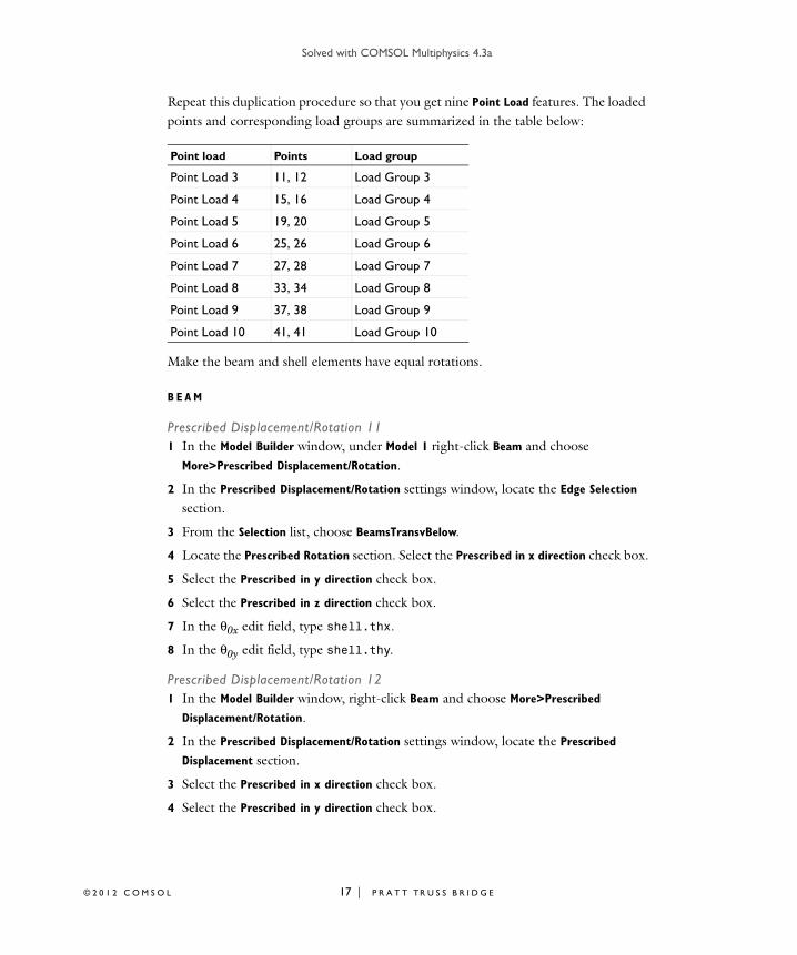
Repeat this duplication procedure so that you get nine Point Load features. The loaded points and corresponding load groups are summarized in the table below:
Point load Points Load group
Point Load 3 11, 12 Load Group 3
Point Load 4 15, 16 Load Group 4
Point Load 5 19, 20 Load Group 5
Point Load 6 25, 26 Load Group 6
Point Load 7 27, 28 Load Group 7
Point Load 8 33, 34 Load Group 8
Point Load 9 37, 38 Load Group 9
Point Load 10 41, 41 Load Group 10
Make the beam and shell elements have equal rotations.
B E A M
Prescribed Displacement/Rotation 111 In the Model Builder window, under Model 1 right-click Beam and choose
More>Prescribed Displacement/Rotation.
2 In the Prescribed Displacement/Rotation settings window, locate the Edge Selection section.
3 From the Selection list, choose BeamsTransvBelow.
4 Locate the Prescribed Rotation section. Select the Prescribed in x direction check box.
5 Select the Prescribed in y direction check box.
6 Select the Prescribed in z direction check box.
7 In the θ0x edit field, type shell.thx.
8 In the θ0y edit field, type shell.thy.
Prescribed Displacement/Rotation 121 In the Model Builder window, right-click Beam and choose More>Prescribed
Displacement/Rotation.
2 In the Prescribed Displacement/Rotation settings window, locate the Prescribed
Displacement section.
3 Select the Prescribed in x direction check box.
4 Select the Prescribed in y direction check box.
M S O L 17 | P R A T T TR U S S B R I D G E

Solved with COMSOL Multiphysics 4.3a
18 | P R A
5 Select the Prescribed in z direction check box.
6 Locate the Prescribed Rotation section. Select the Prescribed in x direction check box.
7 Select the Prescribed in y direction check box.
8 Select the Prescribed in z direction check box.
9 In the θ0x edit field, type shell.thx.
10 In the θ0y edit field, type shell.thy.
11 Select Edge 1 only.
Prescribed Displacement/Rotation 131 Right-click Beam and choose More>Prescribed Displacement/Rotation.
2 In the Prescribed Displacement/Rotation settings window, locate the Prescribed
Displacement section.
3 Select the Prescribed in y direction check box.
4 Select the Prescribed in z direction check box.
5 Locate the Prescribed Rotation section. Select the Prescribed in x direction check box.
6 Select the Prescribed in y direction check box.
7 Select the Prescribed in z direction check box.
8 In the θ0x edit field, type shell.thx.
9 In the θ0y edit field, type shell.thy.
10 Select Edge 78 only.
Set the cross-section data of the different beam types.
Cross Section Data 11 In the Model Builder window, under Model 1>Beam click Cross Section Data 1.
2 In the Cross Section Data settings window, locate the Cross Section Definition section.
3 From the list, choose Common sections.
4 From the Section type list, choose Box.
5 In the hy edit field, type 200[mm].
6 In the hz edit field, type 200[mm].
7 In the ty edit field, type 16[mm].
8 In the tz edit field, type 16[mm].
9 Right-click Model 1>Beam>Cross Section Data 1 and choose Rename.
T T TR U S S B R I D G E © 2 0 1 2 C O M S O L

Solved with COMSOL Multiphysics 4.3a
© 2 0 1 2 C O
10 Go to the Rename Cross Section Data dialog box and type Cross Section Main in the New name edit field.
11 Click OK.
Section Orientation 11 In the Section Orientation settings window, locate the Section Orientation section.
2 From the Orientation method list, choose Orientation vector.
3 In the V table, enter the following settings:
Cross Section Data 21 In the Model Builder window, right-click Beam and choose Cross Section Data.
2 In the Cross Section Data settings window, locate the Edge Selection section.
3 From the Selection list, choose BeamsDiag.
4 Locate the Cross Section Definition section. From the list, choose Common sections.
5 From the Section type list, choose Box.
6 In the hy edit field, type 200[mm].
7 In the hz edit field, type 100[mm].
8 In the ty edit field, type 12.5[mm].
9 In the tz edit field, type 12.5[mm].
10 Right-click Model 1>Beam>Cross Section Data 2 and choose Rename.
11 Go to the Rename Cross Section Data dialog box and type Cross Section Diagonals in the New name edit field.
12 Click OK.
Section Orientation 11 In the Section Orientation settings window, locate the Section Orientation section.
2 From the Orientation method list, choose Orientation vector.
3 In the V table, enter the following settings:
0 x
1 y
0 z
0 x
1 y
0 z
M S O L 19 | P R A T T TR U S S B R I D G E

Solved with COMSOL Multiphysics 4.3a
20 | P R A
Cross Section Data 31 In the Model Builder window, right-click Beam and choose Cross Section Data.
2 In the Cross Section Data settings window, locate the Edge Selection section.
3 From the Selection list, choose BeamsTransvBelow.
4 Locate the Cross Section Definition section. From the list, choose Common sections.
5 From the Section type list, choose H-profile.
6 In the hy edit field, type 96[mm].
7 In the hz edit field, type 100[mm].
8 In the ty edit field, type 8[mm].
9 In the tz edit field, type 5[mm].
10 Right-click Model 1>Beam>Cross Section Data 3 and choose Rename.
11 Go to the Rename Cross Section Data dialog box and type Cross Section Transv Below in the New name edit field.
12 Click OK.
Section Orientation 11 In the Section Orientation settings window, locate the Section Orientation section.
2 From the Orientation method list, choose Orientation vector.
3 In the V table, enter the following settings:
Cross Section Data 41 In the Model Builder window, right-click Beam and choose Cross Section Data.
2 In the Cross Section Data settings window, locate the Edge Selection section.
3 From the Selection list, choose BeamsTransvAbove.
4 Locate the Cross Section Definition section. From the list, choose Common sections.
5 In the hy edit field, type 100[mm].
6 In the hz edit field, type 25[mm].
7 Right-click Model 1>Beam>Cross Section Data 4 and choose Rename.
8 Go to the Rename Cross Section Data dialog box and type Cross Section Transv Above in the New name edit field.
0 x
0 y
1 z
T T TR U S S B R I D G E © 2 0 1 2 C O M S O L

Solved with COMSOL Multiphysics 4.3a
© 2 0 1 2 C O
9 Click OK.
Section Orientation 11 In the Section Orientation settings window, locate the Section Orientation section.
2 From the Orientation method list, choose Orientation vector.
3 In the V table, enter the following settings:
Add the self weight of the beams.
Edge Load 11 In the Model Builder window, right-click Beam and choose Edge Load.
2 In the Edge Load settings window, locate the Edge Selection section.
3 From the Selection list, choose All edges.
4 Locate the Force section. From the Load type list, choose Edge load defined as force
per unit volume.
5 In the F table, enter the following settings:
M E S H 1
1 In the Model Builder window, under Model 1 click Mesh 1.
2 In the Mesh settings window, locate the Mesh Settings section.
3 From the Element size list, choose Extremely fine.
4 Click the Build All button.
S T U D Y 1
Step 1: Stationary1 In the Model Builder window, under Study 1 click Step 1: Stationary.
2 In the Stationary settings window, click to expand the Study Extensions section.
3 Select the Define load cases check box.
1 x
0 y
0 z
0 x
0 y
-g_const*beam.rho z
M S O L 21 | P R A T T TR U S S B R I D G E
Solved with COMSOL Multiphysics 4.3a
22 | P R A
4 Click Add.
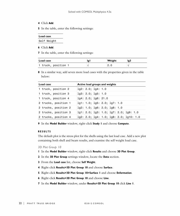
5 In the table, enter the following settings:
6 Click Add.
7 In the table, enter the following settings:
8 In a similar way, add seven more load cases with the properties given in the table below:
9 In the Model Builder window, right-click Study 1 and choose Compute.
R E S U L T S
The default plot is the stress plot for the shells using the last load case. Add a new plot containing both shell and beam results, and examine the self weight load case.
3D Plot Group 101 In the Model Builder window, right-click Results and choose 3D Plot Group.
2 In the 3D Plot Group settings window, locate the Data section.
3 From the Load case list, choose Self Weight.
4 Right-click Results>3D Plot Group 10 and choose Surface.
5 Right-click Results>3D Plot Group 10>Surface 1 and choose Deformation.
6 Right-click Results>3D Plot Group 10 and choose Line.
7 In the Model Builder window, under Results>3D Plot Group 10 click Line 1.
Load case
Self Weight
Load case lg1 Weight lg3
1 truck, position 1 √ 2.0 √
Load case Active load groups and weights
1 truck, position 2 lg2: 2.0; lg4: 1.0
1 truck, position 3 lg3: 2.0; lg5: 1.0
1 truck, position 4 lg4: 2.0; lg6: 21.0
2 trucks, position 1 lg1: 1.0; lg5: 2.0; lg7: 1.0
2 trucks, position 2 lg2: 1.0; lg6: 2.0; lg8: 1.0
2 trucks, position 3 lg1: 2.0; lg3: 1.0; lg7: 2.0; lg9: 1.0
2 trucks, position 4 lg2: 2.0; lg4: 1.0; lg8: 2.0; lg10: 1.0
T T TR U S S B R I D G E © 2 0 1 2 C O M S O L
Solved with COMSOL Multiphysics 4.3a
© 2 0 1 2 C O
8 In the Line settings window, click Replace Expression in the upper-right corner of the Expression section. From the menu, choose Beam>Displacement>Total displacement
(beam.disp).
You can indicate the dimensions of the beams by drawing them with a size depending on the radius of gyration.
9 Locate the Coloring and Style section. From the Line type list, choose Tube.
10 In the Tube radius expression edit field, type mod1.beam.rgy+mod1.beam.rgz.
11 Click to expand the Inherit Style section. From the Plot list, choose Surface 1.
12 In the Model Builder window, under Results>3D Plot Group 10 click Surface 1.
13 In the Surface settings window, click to expand the Range section.
14 Select the Manual color range check box.
15 In the Maximum edit field, type 0.05.
16 In the Model Builder window, under Results>3D Plot Group 10 right-click Line 1 and choose Deformation.
17 Click the Plot button.
18 In the 3D Plot Group settings window, locate the Plot Settings section.
19 Clear the Plot data set edges check box.
20 Click the Plot button.
21 In the Model Builder window, under Results>3D Plot Group 10 click Line 1.
22 In the Line settings window, click Replace Expression in the upper-right corner of the Expression section. From the menu, choose Beam>Section forces>Local axial force
(beam.Nxl).
23 In the Model Builder window, under Results>3D Plot Group 10 click Line 1.
24 In the Line settings window, locate the Inherit Style section.
25 From the Plot list, choose None.
26 Click to expand the Range section. Select the Manual color range check box.
27 In the Minimum edit field, type -9e5.
28 In the Maximum edit field, type 9e5.
29 Locate the Coloring and Style section. From the Color table list, choose Wave.
30 In the Model Builder window, under Results>3D Plot Group 10 right-click Surface 1 and choose Disable.
You can also look at the stress results for the different load cases including the truck weight.
M S O L 23 | P R A T T TR U S S B R I D G E

Solved with COMSOL Multiphysics 4.3a
24 | P R A
Stress Top (shell)1 In the Model Builder window, under Results click Stress Top (shell).
2 In the 3D Plot Group settings window, locate the Data section.
3 From the Load case list, choose 2 trucks, position 4.
4 Click the Plot button.
Create an animation of the trucks passing the bridge.
5 Click the Player button on the main toolbar.
You can easily remove unused plots to clean up the structure in the Results tree. An alternative could have been to deselect Generate default plots in the Study feature, but then you would have needed to create the current plot manually.
6 In the Model Builder window, select Results>Stress Bottom (shell) 1, hold down the Shift key, and then select Results>Torsion Moment (beam) 1. Right click and choose Delete.
R O O T
In the Model Builder window, right-click the root node and choose Add Study.
M O D E L W I Z A R D
1 Go to the Model Wizard window.
2 Find the Studies subsection. In the tree, select Preset Studies for Selected
Physics>Eigenfrequency.
3 Click Finish.
S T U D Y 2
Step 1: Eigenfrequency1 In the Model Builder window, under Study 2 click Step 1: Eigenfrequency.
2 In the Eigenfrequency settings window, locate the Study Settings section.
3 In the Desired number of eigenfrequencies edit field, type 12.
4 In the Model Builder window, right-click Study 2 and choose Compute.
Select the first mode involving the roadway.
R E S U L T S
Mode Shape (shell)1 In the Model Builder window, under Results click Mode Shape (shell).
T T TR U S S B R I D G E © 2 0 1 2 C O M S O L

Solved with COMSOL Multiphysics 4.3a
© 2 0 1 2 C O
2 In the 3D Plot Group settings window, locate the Data section.
3 From the Eigenfrequency list, choose 3.325624.
4 In the Model Builder window, expand the Mode Shape (shell) node.
Mode Shape (beam)In the Model Builder window, expand the Results>Mode Shape (beam) node.
Mode Shape (shell)1 Right-click Line 1 and choose Copy.
2 In the Model Builder window, under Results right-click Mode Shape (shell) and choose Paste Line.
3 In the Line settings window, locate the Inherit Style section.
4 From the Plot list, choose Surface 1.
5 In the Model Builder window, expand the Results>Mode Shape (shell)>Surface 1 node, then click Deformation.
6 In the Deformation settings window, locate the Scale section.
7 Select the Scale factor check box.
8 In the associated edit field, type 0.2.
9 In the Model Builder window, under Results>Mode Shape (shell) click Surface 1.
10 In the Surface settings window, locate the Range section.
11 Select the Manual color range check box.
12 In the Maximum edit field, type 4.
13 Click the Plot button.
M S O L 25 | P R A T T TR U S S B R I D G E

Solved with COMSOL Multiphysics 4.3a
26 | P R A
T T TR U S S B R I D G E © 2 0 1 2 C O M S O L