Epsilon Equitable Partitions based Approach for Role& Positional Analysis of Social Networks

A THESIS

submitted by

PRATIK VINAY GUPTE

for the award of the degree

of

MASTER OF SCIENCE(by Research)

DEPARTMENT OF COMPUTER SCIENCE AND ENGINEERINGINDIAN INSTITUTE OF TECHNOLOGY MADRAS

JUNE 2015

THESIS CERTIFICATE

This is to certify that the thesis entitled Epsilon Equitable Partitions based Approach

for Role & Positional Analysis of Social Networks, submitted by Pratik Vinay

Gupte, to the Indian Institute of Technology, Madras, for the award of the degree

of Master of Science (by Research), is a bona fide record of the research work

carried out by him under my supervision. The contents of this thesis, in full or in

parts, have not been submitted to any other Institute or University for the award

of any degree or diploma.

Dr. B. RavindranResearch GuideAssociate ProfessorDept. of Computer Science and Engineering Date:IIT Madras,Chennai 600 036

To my teachers

i

ACKNOWLEDGEMENTS

First and foremost, I would like to express my sincere gratitude to my advisor,

Dr. B. Ravindran Sir. I do not think it would have been possible for this work to

assume its present form without his advice and guidance at all stages. His energy,

enthusiasm, and generosity has helped me both personally and professionally.

I thank the members of General Test Committee, Dr. S. Krishnamoorthy, Dr.

Sutanu Chakraborti and Dr. David Koilpillai for their constructive feedback during

my interactions with them. I also wish to thank Dr. Ashish V. Tendulkar who

graciously accommodated me in his busy schedules when I needed his guidance

on experiments related to biological datasets.

I thank all my teachers for instilling in me the reverence for knowledge.

My thanks to all members of the Computer science department for providing

a stimulating atmosphere for conducting research. I also thank the entire IIT

Madras system for the rewarding influence it had on me.

I am thankful to all members of DON lab and RISE lab for all the great times

we had, inside and outside the lab.

Numerous collaborators, colleagues and friends have helped me in so many

ways during my life as a graduate student. I refrain from naming each one, lest I

omit somebody. The last few years have formed several productive collaborations

and wonderful friendships, which I am sure will last for long periods to come.

The moral support provided by my family has been a constant source of strength

throughout my life.

ii

ABSTRACT

In social network analysis, the fundamental idea behind the notion of position is

to discover actors who have similar structural signatures. Positional analysis of

social networks involves partitioning the actors into disjoint sets using a notion of

equivalence which captures the structure of relationships among actors. Classical

approaches to Positional Analysis, such as Regular equivalence and Equitable

Partitions, are too strict in grouping actors and often lead to trivial partitioning

of actors in real world networks. An ε-Equitable Partition (εEP) of a graph

is a useful relaxation to the notion of structural equivalence which results in

meaningful partitioning of actors. All these methods assume a single role per

actor, actors in real world tend to perform multiple roles. For example, a Professor

can possibly be in a role of “Advisor” to his PhD students, but in a role of

“Colleague” to other Professors in his department. In this thesis we propose

ε-equitable partitions based approaches to perform scalable positional analysis and

to discover positions performing multiple roles. First, we propose and implement

a new scalable distributed algorithm based on MapReduce methodology to find

εEP of a graph. Empirical studies on random power-law graphs show that our

algorithm is highly scalable for sparse graphs, thereby giving us the ability to

study positional analysis on very large scale networks. Second, we propose a

new notion of equivalence for performing positional analysis of networks using

multiple ε-equitable partitions. These multiple partitions give us a better bound on

iii

identifying equivalent actor “positions” performing multiple “roles”. Evaluation

of our methods on multi-role ground-truth networks and time evolving snapshots

of real world social graphs show the importance of epsilon equitable partitions for

discovering positions performing multiple roles and in studying the evolution of

actors and their ties.

KEYWORDS: Equitable Partition, Positional Analysis, Multiple Role

Analysis, Structural Equivalence, Distributed Graph

Partitioning

iv

TABLE OF CONTENTS

ACKNOWLEDGEMENTS ii

ABSTRACT iii

LIST OF TABLES ix

LIST OF FIGURES xi

LIST OF SYMBOLS xiii

ABBREVIATIONS xiv

1 Introduction 1

1.1 Motivation . . . . . . . . . . . . . . . . . . . . . . . . . . . . . . . . 2

1.2 Organization of the Thesis . . . . . . . . . . . . . . . . . . . . . . . 3

1.3 Major Contributions of the Thesis . . . . . . . . . . . . . . . . . . . 4

2 Overview of Role and Positional Analysis 6

2.1 Position and Role . . . . . . . . . . . . . . . . . . . . . . . . . . . . 6

2.2 Mathematical Preliminaries . . . . . . . . . . . . . . . . . . . . . . 7

2.2.1 Partition and Ordered Partition . . . . . . . . . . . . . . . . 8

2.3 Classical Methods of Role and Positional Analysis . . . . . . . . . 10

2.3.1 Structural Equivalence . . . . . . . . . . . . . . . . . . . . . 10

2.3.2 Regular Equivalence . . . . . . . . . . . . . . . . . . . . . . 13

2.3.3 Automorphisms . . . . . . . . . . . . . . . . . . . . . . . . 19

2.3.4 Equitable Partition . . . . . . . . . . . . . . . . . . . . . . . 20

2.3.5 Computing Equitable Partition . . . . . . . . . . . . . . . . 21

v

2.4 Stochastic Blockmodels . . . . . . . . . . . . . . . . . . . . . . . . . 23

2.5 Overview of ε-Equitable Partition . . . . . . . . . . . . . . . . . . . 24

2.5.1 ε-Equitable Partition . . . . . . . . . . . . . . . . . . . . . . 24

2.5.2 Advantages of ε-Equitable Partition . . . . . . . . . . . . . 28

2.5.3 Algorithm for finding an εEP from [1] . . . . . . . . . . . . 29

3 Scalable Positional Analysis: Fast and Scalable Epsilon Equitable PartitionAlgorithm 31

3.1 Motivation . . . . . . . . . . . . . . . . . . . . . . . . . . . . . . . . 31

3.2 Fast ε-Equitable Partition . . . . . . . . . . . . . . . . . . . . . . . . 32

3.2.1 Description of Fast εEP Algorithm . . . . . . . . . . . . . . 33

3.2.2 A note on running time complexity of the Fast εEP Algorithm 36

3.3 Scalable and Distributed ε-Equitable Partition . . . . . . . . . . . 37

3.3.1 Overview of MapReduce . . . . . . . . . . . . . . . . . . . 37

3.3.2 Logical/Programming View of the MR Paradigm . . . . . . 38

3.3.3 Parallel ε-Equitable Partition . . . . . . . . . . . . . . . . . 39

3.4 Experimental Evaluation . . . . . . . . . . . . . . . . . . . . . . . . 41

3.4.1 Evaluation on an Example Toy Network . . . . . . . . . . . 41

3.4.2 Datasets used for Dynamic Analysis . . . . . . . . . . . . . 43

3.4.3 Evaluation Methodology . . . . . . . . . . . . . . . . . . . 46

3.4.4 Results of Dynamic Analysis . . . . . . . . . . . . . . . . . 56

3.4.5 Scalability Analysis of the Parallel εEP Algorithm . . . . . 62

3.5 Conclusions . . . . . . . . . . . . . . . . . . . . . . . . . . . . . . . 64

4 Discovering Positions Performing Multiple Roles: Multiple EpsilonEquitable Partitions 65

4.1 On Non-Uniqueness of ε-Equitable Partition . . . . . . . . . . . . 66

4.2 Motivation . . . . . . . . . . . . . . . . . . . . . . . . . . . . . . . . 70

4.3 Algorithm for finding Multiple Epsilon Equitable Partitions . . . 71

4.3.1 Implementation of the MεEPs Algorithm . . . . . . . . . . 74

vi

4.4 Actor-Actor Similarity Score . . . . . . . . . . . . . . . . . . . . . . 79

4.5 Definition of a “Position” in Multiple ε-Equitable Partitions . . . 81

4.5.1 Hierarchical Clustering . . . . . . . . . . . . . . . . . . . . 81

4.5.2 Positional Equivalence in Multiple ε-Equitable Partitions . 83

4.6 Experimental Evaluation . . . . . . . . . . . . . . . . . . . . . . . . 87

4.6.1 Datasets used for Evaluation . . . . . . . . . . . . . . . . . 87

4.6.2 Evaluation Methodology . . . . . . . . . . . . . . . . . . . 91

4.6.3 Results . . . . . . . . . . . . . . . . . . . . . . . . . . . . . . 96

4.7 Conclusions and Discussion . . . . . . . . . . . . . . . . . . . . . . 114

5 Conclusions and Future Work 115

5.1 Conclusions . . . . . . . . . . . . . . . . . . . . . . . . . . . . . . . 115

5.2 Future Scope of Work . . . . . . . . . . . . . . . . . . . . . . . . . . 116

5.2.1 Structural Partitioning of Weighted Graphs . . . . . . . . . 116

5.2.2 Scalable Equitable Partitioning . . . . . . . . . . . . . . . . 120

A Partition Similarity Score 121

A.1 Mathematical Preliminaries . . . . . . . . . . . . . . . . . . . . . . 121

A.2 Simplified Representation of the Partition Similarity Score . . . . 123

A.3 MapReduce Algorithm to Compute the Partition Similarity Score 124

References 126

LIST OF TABLES

3.1 Dry Run of the Fast εEP Algorithm on the TA Network of Figure 2.5 36

3.2 Facebook Dataset Details . . . . . . . . . . . . . . . . . . . . . . . . . 45

3.3 Flickr Dataset Details . . . . . . . . . . . . . . . . . . . . . . . . . . . 45

3.4 Percentage of εEP Overlap using the Partition Similarity Score forTime Evolving Graphs of the Facebook Network . . . . . . . . . . 55

3.5 Computational Aspects of the Scalable EEP Algorithm: Curve FittingResults, ε = 5 . . . . . . . . . . . . . . . . . . . . . . . . . . . . . . . 63

4.1 Node DVs of the TA Network’s Equitable Partition (Figure: 4.1a) in SortedOrder of their Cell Degrees . . . . . . . . . . . . . . . . . . . . . . . . 67

4.2 Non-uniqueness of EEP of a graph. First 1-Equitable Partition . . 68

4.3 Non-uniqueness of EEP of a graph. Second 1-Equitable Partition 69

4.4 Cell degree vectors of πpert. . . . . . . . . . . . . . . . . . . . . . . . 76

4.5 Cell merge sequence for πpert. . . . . . . . . . . . . . . . . . . . . . 77

4.6 Cell degree vectors of πinit. . . . . . . . . . . . . . . . . . . . . . . . 77

4.7 Cell-to-cell mapping between πinit and πpert. . . . . . . . . . . . . . 78

4.8 Cell merge sequence of πpert using DVs of πinit and a mapping. . . 78

4.9 IMDb Dataset Role Distributions . . . . . . . . . . . . . . . . . . . . . 88

4.10 Summer School Dataset Role Distributions . . . . . . . . . . . . . . . . 89

4.11 JMLR Dataset Properties . . . . . . . . . . . . . . . . . . . . . . . . . 90

4.12 DBLP Co-Authorship Network Details . . . . . . . . . . . . . . . . . . 91

4.13 Evaluation on IMDb Co-Cast Network. . . . . . . . . . . . . . . . 96

4.14 Evaluation on Summer School Network. . . . . . . . . . . . . . . . 98

4.15 Evolution in JMLR Co-Citation Network with MεEPs SL Epsilon=6 . . 104

4.16 Evolution in JMLR Co-Citation Network with MεEPs CL Epsilon=6 . . 104

4.17 Evolution in JMLR Co-Citation Network with MεEPs SL Epsilon=4 . . 105

viii

4.18 Evolution in JMLR Co-Citation Network with MεEPs CL Epsilon=4 . . 105

4.19 Evolution in JMLR Co-Citation Network with MεEPs SL Epsilon=2 . . 105

4.20 Evolution in JMLR Co-Citation Network with MεEPs CL Epsilon=2 . . 105

5.1 Comparison of Weighted ε-Equitable Partition with MεEPs using the PartitionSimilarity Score (Equation 3.1) for the JMLR Co-Citation Network of Year2007, with Years from 2008→ 2011. . . . . . . . . . . . . . . . . . . . 119

5.2 Comparison of Weighted ε-Equitable Partition with MεEPs using the PartitionSimilarity Score (Equation 3.1) for the JMLR Co-Citation Network of Year2010 with Year 2011. . . . . . . . . . . . . . . . . . . . . . . . . . . . . 119

ix

LIST OF FIGURES

2.1 Example of a “finer” than Relation . . . . . . . . . . . . . . . . . . . . 8

2.2 Example of Structural Equivalence . . . . . . . . . . . . . . . . . . 11

2.3 Example of Regular Equivalence . . . . . . . . . . . . . . . . . . . 13

2.4 Example graph for equivalence given by REGE . . . . . . . . . . . 16

2.5 TA Network . . . . . . . . . . . . . . . . . . . . . . . . . . . . . . . 28

3.1 Overview of our Lightweight MapReduce Implementation . . . . 42

3.2 TA Network: Evaluation of the Fast Epsilon Equitable PartitionAlgorithm 4 . . . . . . . . . . . . . . . . . . . . . . . . . . . . . . . 43

3.3 Dataset Properties of the Facebook Graph . . . . . . . . . . . . . . 44

3.4 Dataset Properties of the Flickr Graph . . . . . . . . . . . . . . . . 45

3.5 Co-evolving Node Pairs for Facebook Graph G1 → G2. (a) Difference ofBetweenness Centrality. (b) Difference of Normalized Degree Centrality. 49

3.5 Co-evolving Node Pairs for Facebook Graph G1 → G2. (c) Difference ofShapley Value Centrality. (d) Difference of Triangles. . . . . . . . . . . 50

3.6 Co-evolving Node Pairs for Facebook Graph G2 → G3. (a) Difference ofBetweenness Centrality. (b) Difference of Normalized Degree Centrality. 51

3.6 Co-evolving Node Pairs for Facebook Graph G2 → G3. (c) Difference ofShapley Value Centrality. (d) Difference of Triangles. . . . . . . . . . . 52

3.7 Co-evolving Node Pairs for Facebook Graph G1 → G3. (a) Difference ofBetweenness Centrality. (b) Difference of Normalized Degree Centrality. 53

3.7 Co-evolving Node Pairs for Facebook Graph G1 → G3. (c) Differenceof Shapley Value Centrality. (d) Difference of Triangles. . . . . . . 54

3.8 Co-evolving Node Pairs for Flickr graph G1 → G2. (a) Difference ofShapley Value Centrality. (b) Difference of Triangles. . . . . . . . . 55

3.9 Position Size Distribution for Facebook Graph G3. (a) Degree Partition.(b) Equitable Partition. . . . . . . . . . . . . . . . . . . . . . . . . . 59

3.9 Position Size Distribution for Facebook Graph G3. (c) εEP, ε = 1. (d)εEP, ε = 2. . . . . . . . . . . . . . . . . . . . . . . . . . . . . . . . . 60

x

3.9 Position Size Distribution for Facebook Graph G3. (e) εEP, ε = 4. (f)εEP, ε = 8. . . . . . . . . . . . . . . . . . . . . . . . . . . . . . . . . 61

3.10 Parallel εEP Algorithm: Scalability Curve . . . . . . . . . . . . . . 63

3.11 Sequential versus Parallel εEP Algorithm . . . . . . . . . . . . . . 64

4.1 TA Network: Multiple Epsilon Equitable Partitions . . . . . . . . 66

4.2 MεEPs Implementation Example . . . . . . . . . . . . . . . . . . . 75

4.3 Example of Actor-Actor Similarity . . . . . . . . . . . . . . . . . . 80

4.4 Example of Linkage Criteria for HAC . . . . . . . . . . . . . . . . 82

4.5 Best Level to cut the Dendrogram Tree . . . . . . . . . . . . . . . . 85

4.6 IMDb Co-Cast Network Degree Distribution . . . . . . . . . . . . 89

4.7 DBLP Co-Authorship Network Degree Distribution . . . . . . . . 91

4.8 Heatmap of Rearranged Actor-Actor Distance Matrix of the SummerSchool Network . . . . . . . . . . . . . . . . . . . . . . . . . . . . . 100

4.9 Comparison of Partition Similarity Score for JMLR Co-Citation Network 104

4.10 Co-Evolution of Actor-Actor Ties for JMLR Co-Authorship Network 106

4.11 Co-evolving Node Pairs for DBLP Co-Authorship Graph from Year 2008→2013. (a) Difference of Betweenness Centrality. (b) Difference of ClosenessCentrality. . . . . . . . . . . . . . . . . . . . . . . . . . . . . . . . . . 108

4.11 Co-evolving Node Pairs for DBLP Co-Authorship Graph from Year2008→ 2013. (c) Difference of Triangles. . . . . . . . . . . . . . . . 109

4.12 Position Size Distribution for DBLP Co-Authorship Graph for Year2013. (a) Equitable Partition. (b) MεEPs Complete-link, ε = 2. . . 110

4.12 Position Size Distribution for DBLP Co-Authorship Graph for Year 2013.(c) MεEPs Single-link, ε = 2. (d) MεEPs Complete-link, ε = 6. . . . . . . 111

4.12 Position Size Distribution for DBLP Co-Authorship Graph for Year2013. (e) MεEPs Single-link, ε = 6. (f) εEP, ε = 6. . . . . . . . . . . 112

4.12 Position Size Distribution for DBLP Co-Authorship Graph for Year2013. (g) Stochastic Blockmodel. (h) Degree Partition. . . . . . . . 113

5.1 Example Weighted Equitable Partition . . . . . . . . . . . . . . . . 117

5.2 Example Weighted Epsilon Equitable Partition . . . . . . . . . . . 118

xi

LIST OF SYMBOLS

4 The symmetric set difference operator

∩ The set intersection operator

∪ The set union operator

ε The value of relaxation allowed

≡ The equivalence relation

γ The power-law exponent

µ(π) The mean-of-mean cell distance of partition π

−−→deg(v) The degree vector of vertex v

π The partition of vertex set

πinit The ordered equitable partition with initial cell ordering

πpert The ordered equitable partition with permuted cell ordering

4 The finer than relation

~rv The role label vector of vertex v

at The property value of vertex a at time t

at+δt The property value of vertex a at time t + δt

xii

ca The current active cell

ci The ith cell/block of a partition

cooc(a, b) The co-occurrence value of nodes a and b

deg(vi, c j) The degree of vertex vi to cell c j

dist(a, b) The distance between nodes a and b

E The edge set of a graph

G The graph

Gt The graph at time t

Gt+δt The graph at time t + δt

sim(π1, π2) The similarity score between partitions π1 and π2

sim(a, b) The similarity between nodes a and b

V The vertex set of a graph

Z The hierarchical clustering linkage data structure

xiii

ABBREVIATIONS

EP Equitable Partition

εEP/EEP ε-Equitable Partition

MεEPs/MEEPs Multiple ε-Equitable Partitions

SNA Social Network Analysis

PA Positional Analysis

SE Structural Equivalence

RE Regular Equivalence

DV Degree Vector

DP Degree Partition

SBM Stochastic Blockmodel

MR MapReduce

HC Hierarchical Clustering

HAC Hierarchical Agglomerative Clustering

CL Complete-link

SL Single-link

IMDb Internet Movie Database

WεEP Weighted ε-Equitable Partition

xiv

CHAPTER 1

Introduction

In social network analysis, the notions of social position and social role have

been fundamental to the structural analysis of networks. These dual notions

discover actors who have similar structural signatures. This involves identifying

social position as collection of actors who are similar in their ties with others and

modelling social roles as system of ties between actors or between positions. As

an example, head coaches in different football teams occupy the position manager

by the virtue of the similar kind of relationship with players, assistant coaches,

medical staff and the team management. It might happen that an individual coach

at the position manager may or may not have interaction with other coaches at

the same position. Further, the actors at the position manager can be in a role

of “Coach” to actors at the position player or a “Colleague” to the actors at the

position assistant coach. Similarly, the actors at position medical staff can be in a

role of “Physiotherapist” or a “Doctor” to actors at the position player. Positional

Analysis (PA) of social networks involves partitioning the actors into disjoint sets

using a notion of equivalence which captures the structure of relationships among

actors. While PA is a very intuitive way of understanding interactions in networks,

this hasn’t been widely studied to model multiple roles performed by actors, neither

has it been studied for large networks due to the difficulty in developing tractable

algorithms. In this thesis, we propose ε-equitable partition (εEP) based positional

analysis approaches for the two problems as follows:

• Scalable Positional Analysis: We propose a new algorithm with better

heuristics to find the ε-equitable partition of a graph and focus on scaling

this algorithm. We present the results of our algorithm on time evolving

snapshots of the facebook and flickr social graphs. Results show the

importance of positional analysis on large dynamic networks.

• Discovering Positions Performing Multiple Roles: We propose a new

notion of equivalence for performing PA of social networks. Given a network,

we find its Multiple ε-Equitable Partitions (MεEPs) to analyze multiple roles.

These multiple partitions give us a better bound on identifying equivalent

actor “positions” performing multiple “roles”. Evaluation of our method on

multi-role ground-truth networks and time evolving snapshots of real world

social graphs shows the importance of multiple ε equitable partitions for

discovering positions performing multiple roles and also in studying the

evolution of actors and their ties.

1.1 Motivation

The key element in finding positions, which aid in the meaningful interpretation of

the data is the notion of equivalence used to partition the network. Classical methods

of finding equivalence like structural equivalence [2], regular equivalence [3],

automorphisms [4] and equitable partition [5, 6] often lead to trivial partitioning

of the actors in the network. An ε-equitable partition (εEP) [7] is a notion of

equivalence, which has many advantages over the classical methods. εEP allows

a leeway of ε in the number of connections the actors at a same position can have

2

with the actors at another position. In the Indian movies dataset from IMDb,

authors in [7] have shown that actors who fall in the same block of the partition,

tend to have acted in similar kinds of movies. Further, the authors also show that

people who belong to a same position of an εEP tend to evolve similarly. In social

networks, tagging people who belong to the same position has potentially many

applications, both from business and individual perspective, such as, position

based targeted promotions, ability to find anomalies, user churn prediction and

personalised recommendations.

Though efficient graph partition refinement techniques and their application in

finding the regular equivalence of a graph are well studied in the graph theoretic

literature [8, 9], the application of these techniques for doing positional analysis

of very large social graphs and networks is so far unknown. In this thesis, we

propose a new algorithm to find the ε-equitable partition of a graph and focus on

scaling this algorithm.

Further, an observation we made from ε-equitable partitioning method was

that the εEP of a graph is not unique and many such partitions exist. In this

thesis, we exploit these multiple ε-equitable partitions to analyze multiple roles

and positions. We define a new notion of equivalence based on these multiple

εEPs to perform PA of social networks.

1.2 Organization of the Thesis

• Chapter 2 covers detailed background work on Role and Positional Analysis

in Social Network Analysis (SNA) literature.

3

• Chapter 3 presents our contribution of a new, scalable and distributed algorithm

for finding ε-equitable partition of a graph. We discuss about the algorithm

complexity, implementation, evaluation methodology and our contribution

on parallelizing the algorithm using MapReduce paradigm.

• In Chapter 4 we discuss about the non-uniqueness of εEP of a graph and

subsequently propose the notion of Multiple ε- Equitable Partitions (MεEPs)

and an algorithm to find MεEPs for a graph. We present the notion of

Positional Equivalence in MεEPs along with the algorithm, its implementation,

ground-truth network evaluation methodology, dataset details and results on

real world networks.

• Chapter 5 concludes the thesis. A summary of the work and future directions

are provided here. We also present preliminary results on the notion of

structural equivalence for weighted graphs.

1.3 Major Contributions of the Thesis

The major contributions of the thesis are as follows:

• We propose a new algorithm with better heuristics to find the ε-equitable

partition of a graph and implement its scalable distributed algorithm based

on MapReduce methodology [10]. This allows us to study the Positional

Analysis on large dynamic social networks. We have successfully validated

our algorithm with detailed studies on facebook social graph, highlighting the

advantages of doing positional analysis on time evolving social network

4

graphs. We present few results on a relatively large component of the

flickr social network. Further more, the empirical scalability analysis of the

proposed new algorithm shows that the algorithm is highly scalable for

large sparse graphs. We also compare the positions given by our proposed

algorithm with the ones given by the εEP algorithm as proposed in [7] on an

example toy network.

• We propose a new notion of equivalence using multiple ε-equitable partitions

of a graph. These multiple partitions give us a better bound on grouping

actors and better insights into the “roles” of actors. We compute a similarity

score for each actor-pair based on their co-occurrence at a same position across

multiple εEPs. We define a new notion of equivalence using these pairwise

similarity scores to perform agglomerative hierarchical clustering to identify

the set of equivalent actors. Evaluation of our method on multi-role ground

truth IMDb co-cast network shows that our method correctly discovers

positions performing multiple roles; empirical evaluation on time evolving

snapshots of JMLR co-citation and co-authorship graphs shows the importance

of MεEPs in studying the evolution of actors and their ties.

5

CHAPTER 2

Overview of Role and Positional Analysis

The notions of social position and social role have been fundamental to the structural

analysis of networks. These dual notions, are key techniques in identifying actors

which are similarly embedded in a network and in finding out the pattern of

relations, which exist among these similarly embedded actors.

This chapter is organized as follows. Section 2.1 explains the notion of position

and roles. Section 2.2 explains mathematical preliminaries. Section 2.3 introduces

the classical methods of role and positional analysis. Section 2.4 speaks about the

Stochastic Blockmodels approach to positional analysis.

2.1 Position and Role

In SNA, the fundamental idea behind the notion of position is to find out actors

which have similar structural signature in a network. Actors who have same

structural correspondence to other actors in a network are said to occupy same

“position”. On the other hand, the fundamental idea behind the notion of role is to

find out similar pattern of relations among different actors or positions. Actors at

same position tend to perform same “role” to actors at another position [11, 12, 13].

Wasserman and Faust [11] state “key aspect in role and position analysis is:

identifying social position as collection of actors who are similar in their ties with

others and modelling social roles as system of ties between actors or between

positions”.

For example, professors in different universities occupy the position “Professor”

by the virtue of similar kind of relationship with students, research scholars and

other professors. Though individual professors may not know each other. Also,

since the notion of role is dependent formally and conceptually on the notion of

position, in the same example a professor could be in a role of “Guide” to his research

scholars and in the role of a “Colleague” to fellow professors of his department.

2.2 Mathematical Preliminaries

Positional Analysis (PA) [11] of a social network aims to find similarities between

actors (vertices) in the network. It is about dividing set of actors into subsets, such

that actors in a particular subset are structurally similar to other actors. PA tries

to identify actors which are similarly embedded in the network. PA also helps in

analyzing the evolution of networks [14], actors at a particular position tend to

evolve in a similar fashion.

Mathematically, PA is finding a partition of the graph on the basis of some

equivalence relation. The subsequent section (2.3) discusses few important equivalence

relations in detail. Before that, we present few mathematical definitions in the

following subsection (2.2.1).

7

2.2.1 Partition and Ordered Partition

Definition 2.1. (Partition of a graph) Given, graph G ≡ 〈V, E〉, V is the vertex set

and E is the edge set. A partition π is defined as π = {c1, c2, ..., cn} such that,

• ∪ci = V, i = 1 to n and

• i , j⇒ ci ∩ c j = φ

Thus, the definition of a partition of a graph G means that we have non-empty

subsets of the vertex set V, such that all subset pairs are disjoint to each other. These

subsets c1, c2, ..., cn are called cells or blocks∗ of the partition π.

A cell with cardinality of one is called trivial or singleton cell. A partition in

which all the cells are trivial is called the discrete partition. On the other hand, a

partition which has all the vertices in a single cell is called the unit partition.

Finer and Coarser partitions: If π1 and π2 are two partitions, then π1 is finer than

π2 (π1 4 π2) and π2 is coarser than π1, if every cell of π1 is a subset of some cell of

π2 (finer than also includes the case when π1 and π2 are equal). Example,

a b c d 4 b a c d 4 a b c d

Figure 2.1: Example of a “finer” than Relation

A refinement of a non-discrete partition π is an action which gives a partition

π′, such that, every cell of π′ is a subset of some cell of π. Example, the partition

∗In this thesis, we use the terms cell, block and position interchangeably.

8

[{a,b},{c},{d,e}] is a refinement of the partition [{a,b,c},{d,e}], but [{a,b,c,d},{e}] isn’t,

since the cell {a,b,c,d} is not a subset of either of the cells {a,b,c} or {d,e}. Precisely, a

refinement action on a partition π maintains the finer than property.

Definition 2.2. (Ordered partition) Given, a partitionπ and a refinement action R on

π. Suppose, the successive application of R on π leads to partitions πi, πi+1, ..., πi+n

respectively, then we say that each of the πi+1 is an order preserving refinement of πi

(i ∈ 1, 2, ...,n) if and only if the relative order of vertices in each cell is preserved

after the application of the refinement action R. Mathematically, given a partition

π1 = {c1, c2, ..., ci, c j..., cn} and let π2 = {z1, z2, ..., zk, zl, ..., zm} be the partition after the

refinement action R on π1, then we say π2 is an ordered partition of π1 if and only if:

• π2 is finer than π1, and

• if i ≤ j, zk ⊆ ci and zl ⊆ c j; implies k ≤ l.

Example,

Letπ1=[{a}, {b, c, d}], further letπ2=[{a}, {b, c}, {d}] andπ3=[{d}, {a}, {b, c}] be the partitions

ofπ1 after application of two different refinement actions. π2 maintains the relative

cell order w.r.t. the vertices of π1 and hence is an ordered partition of π1, but π3 isn’t,

since the cell {a} is located before the cell containing d (i.e. {b, c, d}) in partition π1.

The set of ordered partitions over the relation “finer” than (4), on the vertex

set V form a partially ordered set, wherein the unique maximal element is the unit

partition and the minimal element being the discrete partition. We call an order

preserving refinement of π as a ordered partition of π.

9

2.3 Classical Methods of Role and Positional Analysis

Historically, the notion of social “role” dates back to Nadel’s work “The Theory of

Social Structure” (1957) [15]. A key idea from Nadel’s work projected the use of

pattern of relations among concrete entities to model social structure, rather than

the use of abstract entities or attributes on these entities. He also suggested that to

model a social structure properly, one needs to aggregate these interaction patterns

in a way which is consistent with their inherent network structure. Nadel’s ideas

were first mathematically formalized by Lorrain and White (1971) [2]. In this

seminal paper, they introduced the notion of Structural Equivalence (SE), which is

discussed in the following subsection (2.3.1).

2.3.1 Structural Equivalence

Two actors are structurally equivalent if they have exactly same set of ties to and

from other actors in the network. Mathematically, SE is defined as follows [2]:

Definition 2.3. (Structural equivalence) Given a graph G ≡ 〈V, E〉, a and b are

structurally equivalent if,

• (a, c) ∈ E if and only if (b, c) ∈ E and

• (c, a) ∈ E if and only if (c, b) ∈ E

Example in Figure 2.2 depicts structurally equivalent nodes in same colours.

The partition of the graph according to SE is [{A,B}, {C,D,E}, {F,G}, {H,I,J}]. It is

10

A

B

C

D

E

F

G

H

I

J

Figure 2.2: Example of Structural Equivalence. Structurally equivalent actors arecoloured in same colour, which are {A,B}, {C,D,E}, {F,G}, {H,I,J}. A and Bare equivalent since they have identical ties with the cell {C,D,E}, same is truefor other cells accordingly.

worth mentioning here that, nodes in same cell connect exactly with same set of

nodes in other cells.

Discussion

Since two structurally equivalent actors exactly connect to identical actors in other

cells, they are perfectly substitutable for each other. Also, they have same set of

node properties like: same degree, same centrality, same number of triangles etc.

Though actor substitutability may make sense in small sized networks (like in

scenarios where systematic redundancy of actors needs to be studied), perfect

SE in real-world networks is often rare and mostly leads to trivial partitioning

of the network. For example in the university scenario, two professors would

be equivalent only if they “guide” exactly same set of research scholars, and are

“colleagues” with exactly same set of individuals.

11

Computing Structural Equivalence

Two structurally equivalent actors will have identical correspondence among

rows (or columns) in their graph adjacency matrix. Since exact SE is rare in

most social networks, measures that estimate an approximate notion of structural

equivalence among two nodes make more sense, i.e. estimating the degree to

which their columns are identical. Burt’s STRUCTURE [16] program achieves this

by computing the values of Euclidean distance among each pair of actors (nodes) in

the network, the program then merges nodes which are within threshold distance

of each other incrementally, until all nodes end up in a single cluster (i.e. performs

hierarchical clustering in an agglomerative fashion). Breiger, Boorman and Arabie

(1975) came up with a divisive hierarchical clustering algorithm CONCOR [17]

to estimate SE. The CONCOR (CONvergence of iterated CORrelations) algorithm

computes the Pearson’s product moment correlation among every pair of rows (or

columns) and divides the data in two sets. The process is repeated over the

iterated correlation matrix and in each iteration, all the sets having more that two

elements are split into two parts.

Sailer in 1979 proposed a way to relax the strict definition of SE, which he called

“structural relatedness” (SR). The notion of SR was paraphrased by John Boyd [18]

as “two points are structurally equivalent if they are related in the same ways to

points that are structurally equivalent”. For example, for two professors to be

equivalent, they need to “guide” some research scholar (as opposed to the same

research scholar in SE), since all research scholars are structurally equivalent. The

ideas from Sailer’s work paved way for notions of equivalence which captured

position and role in a better way, we discuss them in following subsections.

12

2.3.2 Regular Equivalence

White and Reitz [3] proposed the notion of Regular Equivalence (RE). RE is a

widely accepted and studied notion of PA. Two actors are regular equivalent if

they have same set of ties to and from equivalent others. Mathematically, RE is

defined as follows:

Definition 2.4. (Regular equivalence) Given a graph G = 〈V, E〉 and let ≡ be an

equivalence relation on V. Then, ≡ is a regular equivalence if and only if for all a, b,

c and d ∈ V, a ≡ b implies:

• (a, c) ∈ E implies there exists d ∈ V such that (b, d) ∈ E and d ≡ c and

• (c, a) ∈ E implies there exists d ∈ V such that (d, b) ∈ E and d ≡ c.

A

B C D

E F G H I

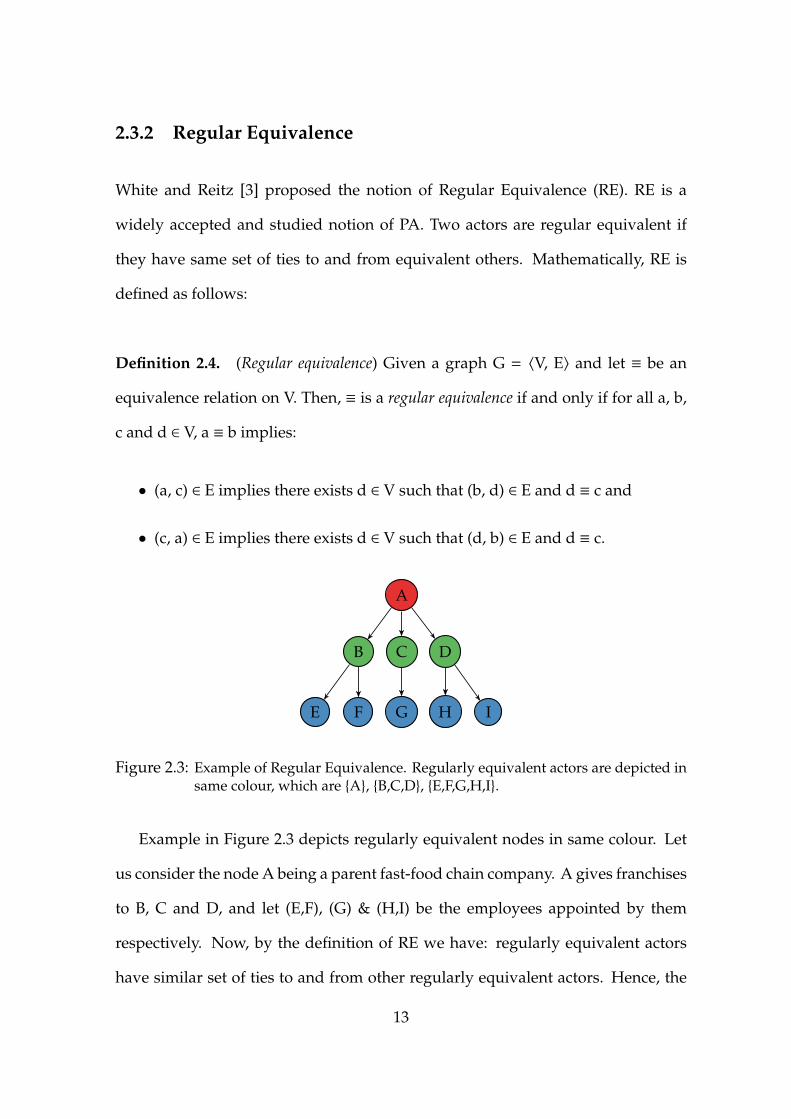
Figure 2.3: Example of Regular Equivalence. Regularly equivalent actors are depicted insame colour, which are {A}, {B,C,D}, {E,F,G,H,I}.

Example in Figure 2.3 depicts regularly equivalent nodes in same colour. Let

us consider the node A being a parent fast-food chain company. A gives franchises

to B, C and D, and let (E,F), (G) & (H,I) be the employees appointed by them

respectively. Now, by the definition of RE we have: regularly equivalent actors

have similar set of ties to and from other regularly equivalent actors. Hence, the

13

positions for actors in example 2.3 are {A} (parent company), {B,C,D} (franchisees),

{E,F,G,H,I} (employees). Here, the RE relation doesn’t try to distinguish among the

employees of B with those of either C or D and vice versa. Here, all the “employees”

belong to a single set because of the virtue of their connections to the “franchisees”

set. SE on the other hand would have distinguished the employees of B, C & D

from each other. An important observation from the “employees” set is that, the RE

relation doesn’t consider the number of connections from other sets, it just considers

the similar nature of ties. Possibly in our example (2.3), the single employee “G”

might have been overloaded in work than others, but RE would have failed to

make that distinction.

Discussion

RE may be understood as partition of actors into classes, s.t. actors who belong to

same class are surrounded by same classes of actors. Marx and Masuch [19] showed

that RE from social networks theory is closely related to the notion of bisimulation

in modal logic from computer science theory. The notion of bisimulation is used

to indicate indistinguishability between two states of two different state transition

systems. Everett and Borgatti (1991) [20] proposed an alternate definition of RE

based on vertex colouring, they coined the term “role colouring” for this definition.

Under this definition, two regularly equivalent vertices belong to same colour class,

and neighbourhoods of each of these vertices (which are also regularly equivalent)

will also belong to different sets of same colour classes respectively.

White and Reitz [3] also defined the notion of multiplex regular equivalence

14

(MPXRE)†. MPXRE requires equivalent actors to have same set (‘bundle’) of

relations with equivalent others. Example, suppose in a 5-relation (R1,R2, ...,R5)

network, node x has outgoing links to node y on R1 and R4, then for any node z to

be equivalent to node x, z needs to have an alter equivalent to node y with exactly

these two relations (R1 and R4). Everett and Borgatti in 1993 [22] extended the

definition of “regular colouring” to directed graphs and networks. In addition to

that, they also define the notion of MPXRE in terms of multiplex regular colouring.

The RE of a graph is not unique. The set of all the regular equivalences of a

graph forms a lattice [23]. The supremum element of the lattice is called maximal

regular equivalence (MRE). In the next subsection we discuss what these multiple

regular equivalences mean.

Computing Regular Equivalence

The earliest algorithm to compute RE was REGE, which was due to the efforts of

White and Reitz from their unpublished manuscripts from University of California,

Irvine archives (1984 and 1985)‡. The idea behind working of REGE algorithm, as

explained by K. Faust [24], could be summarized in 3 steps as follows:

• Step 1: Divide the vertex set into three sets (classes): source, sink and repeaters

(others). If the graph has no distinct source or sink vertices, then the result

has a single equivalence class.

• Step 2: Combine all vertices which have same set of alters w.r.t. other classes.†White and Reitz originally called it ‘bundle equivalence’ and later used the same term to define

a distinct notion (page 208 & 214 of [3]). Hence, we use the term MPXRE as coined by [21] forclarity.‡For more details about these manuscripts, readers are advised to look-up these references [24],

[23] and [21].

15

a

b c

d e f

(a)

a

b c

d e f

(b)

Figure 2.4: Example graph for equivalence given by REGE Algorithm. (a) Undirectedgraph (b) Directed graph

Step 2 is repeated until the equivalence classes do not change.

• Step 3: Output the equivalence classes.

The output of the REGE algorithm for graph in Figure 2.4 (a), is [{a,b,c,d,e,f}].

Whereas, the equivalence classes for the directed graph of Figure 2.4 (b), are

[{a},{b,c},{d,e,f}]. The REGE algorithm finds only the maximal regular equivalence

for any given graph. Also, for the example in Figure 2.4 (a), following are few

partitions which are all valid regular equivalences:

• Partition1 : [{a,b,c,d,e,f}]

• Partition2 : [{a},{b,c},{d,e,f}]

• Partition3 : [{a},{b},{c},{d},{e,f}]

Partition1 being the output of the REGE algorithm (the MRE). Partition3 being

the maximal structural equivalence (MSE). An important point to note here is that, SE

also satisfies the definition of RE. All structurally equivalent actors are regularly

equivalent, but the reverse is not always true. Intuitively, Partition2 might look

like a better fit for the motivation behind RE. Which suggests that both MRE

and MSE fail to capture essence for undirected graphs. On the other hand, the

16

REGE output for the directed graph from Figure 2.4 (b), captures the notion well.

To overcome the disadvantage of a trivial partition under MRE for undirected

graphs, Doreian proposed algorithm for finding RE for symmetric graphs [25].

The idea behind Doreian’s algorithm§ was to split a symmetric structure into two

asymmetric structures by using centrality scores as attribute on nodes, and then use

REGE to find out the RE on each of these asymmetric pairs. Doreian’s algorithm on

the example of Figure 2.4 (a) would still yield Partition3, i.e. the MSE of the graph,

which suggests that Doreian’s algorithm may not always output a ‘best-fit’ RE for

all undirected graphs. Precisely, Doreian’s algorithm finds the RE from the lattice

which is somewhere in between Lorrain and White’s SE [2] and the MRE of White

and Reitz [3]. The reason of its closeness to SE being the dependence of the initial

Doreian’s split on the centrality of the nodes, which (centrality) in turn depends on

the degree of the nodes. Steve Borgatti’s paper from 1988 [26] discusses in detail,

the changes to Doreian’s algorithm, so as to make it more suitable for finding better

and degree independent RE, these ideas influenced the REGE/A algorithm. In the

same paper, Borgatti advocated the need to address the problem of finding the

RE of graph as a hierarchical clustering problem. Rather than finding an unknown

RE (as in the case of Doreian’s algorithm) or finding the MRE (as with REGE), he

proposed looking at the complete tree of the regular equivalences and pick a level,

which suits the level of reduction required based on the data in hand. The REGE/A

algorithm [23] overcomes the disadvantages of Doreian’s split by finding out a MRE

which preserves any point-attribute (node attribute) as chosen by the user, rather

than just the centrality attribute. Few example point-attributes can be centrality

or degree (network theoretic attributes) or even information like education or age

§We use the term Doreian’s split interchangeably to refer to Doreian’s algorithm.

17

(background attributes). The authors also showed the utility of REGE/A algorithm

to “regularize” partitions generated by other equivalences such as the Winship &

Mandel [27] equivalence or orbit partitioning [28]. These partitions are given as

attribute input to REGE/A, the resulting partition is therefore a MRE preserving

that structure. Borgatti and Everett (1993) [21], proposed the algorithm CATREGE

(CATegorical REGE), extending the notion of RE to work with categorical data.

Two actors are regularly equivalent in CATREGE if in addition to the normal

definition of RE, they also relate to equivalent others in the same category. The

input to CATREGE is nominal data, i.e. integer valued adjacency matrix amongst

actors, where the integer values represent relationship in terms of categories. For

example, we can use 1 to represent a close friend, 2 to represent a office colleague

and 3 to represent an acquaintance. It should be noted here that these values do

not capture the strength of a relationship, rather they simply indicate categories.

CATREGE is a divisive HC algorithm, the algorithm starts with all the nodes in the

same equivalence class. First iteration splits the nodes according to basic relational

patterns, which classify the nodes as sources, sinks and repeaters. Second iteration

onwards, the immediate neighbourhoods of the nodes are considered for a split. A

split happens only when their neighbourhoods do not belong to same categories.

Nodes which never split, are perfectly equivalent. CATREGE can also handle data

with multiplex relations. Batagelj et al. [29] proposed the use of a criterion function

which estimates RE and provides a measure of how far a given structure is from

exact regular equivalence, they then use a local optimization procedure to find

a partitioning which minimizes this criterion function. That is, given the final

number of blocks, the algorithm then uses a greedy approach to optimize a cost

function, which estimates the degree to which a partition is regularly equivalent.

18

The authors advocated the efficacy of the local optimization procedure on smaller

graphs as an obvious advantage of the proposed method on larger networks,

though the claim was not supported by any studies. It is very likely, esp. for large

graphs, that a local optimization procedure might terminate at a local minima,

than at a desired global minima. Few authors have also used simulated annealing

[30, 31], tabu search [32, 33] etc. as optimization routines. The use of combinatorial

optimization procedures to approximate RE with user-defined number of classes

makes the problem non-trivial in nature. Roberts and Sheng [34] proved that

the problem of finding 2-role regular equivalence belongs to the class-NP. John

P. Boyd in 2002 [35] proposed a mechanism to estimate the goodness-of-fit of a

given equivalence to regularity, and then used permutation test and an optimization

routine based on the adaptation of Kernighan-Lin variable-depth search algorithm

(Kernighan and Lin [36]) to approximate regular equivalence for a given network.

Kernighan-Lin search works better than greedy search, where local increase in the

fitness score leads to creation of a new class. It is also faster than exhaustive search

over all possible equivalences, but this method also does not guarantee an optimal

solution. The experimental studies based on this method and Boyd & Jonas’s [37]

work on the validity of RE as a measure to precisely model/evaluate social relations

reject regularity decisively, both suggested the need for a new model of defining

equivalence.

2.3.3 Automorphisms

Definition 2.5. (Automorphisms) Given a graph G ≡ 〈V,E〉, an automorphism is a

bijective function f from V → V such that (a, b) ∈ E if and only if ( f (a), f (b)) ∈ E.

19

Discussion

Automorphism can also be understood as an isomorphism from a graph to itself.

Automorphism finds symmetries in the network. The orbits or equivalence classes

of an automorphism group form a partition of the graph and each block of

this partition indicates a position. The problem of finding all automorphically

equivalent vertices is computationally hard (it is not known whether it is NP-complete

or not) and it has been shown to be Graph Isomorphism Complete. However,

efficient graph automorphism solvers like NAutY - No Automorphisms, Yes? [38]

and Saucy [39] exist which are widely used for solving this problem. Automorphism

is also a strict notion for position as it is a bijective function. Real world networks

are quite irregular and hence existence of symmetries is very rare. In the hospital

scenario, two doctors will be automorphically equivalent only if they relate to

the same number of patients, nurses, and colleagues in the same way. Thus

automorphism too fails to characterize the real world notion of similarity.

2.3.4 Equitable Partition

Definition 2.6. (Equitable partition) A partition π = {c1, c2, ..., cn} on the vertex set

V of graph G is said to be equitable [5] if,

for all 1 ≤ i, j ≤ n, deg(u, c j) = deg(v, c j) for all u, v ∈ ci (2.1)

where,

deg(vi, c j) = sizeo f {vk | (vi, vk) ∈ E and vk ∈ c j} (2.2)

20

The term deg(vi, c j) denotes the number of vertices in cell c j adjacent to the vertex

vi. Here, cell c j denotes a position and therefore deg(vi, c j) means the number of

connections the actor vi has to the position c j.

The equitable partition (EP) for a toy TA Network of Figure 2.5(a) is shown

in Figure 2.5(c). EP leads to a trivial partitioning of the network. The EP for

this network has 7 positions, it treats each of the TAs and their respective student

groups separate from each other.

Discussion

Equitable partitions are relaxations of automorphism since the partitions formed

by automorphism are always equitable but the reverse is not true. Polynomial

time algorithms exist for finding the coarsest equitable partition of a graph [5]. It

can be observed that equitable partition is a regular partition with an additional

constraint that the number of connections to the neighbouring positions should be

equal for equivalent nodes. This constraint is too strict for complex large graphs

and hence results in trivial partitioning. For example, in the hospital scenario, two

doctors would be equivalent only if, say one of them interacts with n1 nurses, n2

other doctors and n3 patients, then the other also is connected to n1 nurses, n2 other

doctors and n3 patients.

2.3.5 Computing Equitable Partition

The procedure to find the equitable partition of a graph is given in Algorithm 1.

Given the initial colouring of vertices, the output of the procedure is the coarsest

equitable partition of the input graph. The initial colouring of vertices is an user

21

defined input to the equitable partition algorithm. Please note that, we start with

the unit partition of the vertex set in all the experiments reported in this thesis.

Algorithm 1 Equitable RefinerInput: graph G, coloured partition πOutput: Equitable partition R(G,π)

1: f : V→N2: active = indices(π)3: while (active , φ) do4: idx = min(active)5: active = active r {idx}6: f (u) = degg(u, π[idx]) ∀u ∈ V7: π′ = split(π, f )8: active = active ∪ [ordered indices of new split cells from π′, while replacing

(in place) the indices from π which were split]9: π = π′

10: end while11: return π

Equitable Refinement Function R The key element in the equitable refinement

function illustrated in Algorithm 1 is the procedure split.

split takes as input an ordered partition π on V and a function f , which maps every

vertex u ∈ V to its degree to a subset ca ⊆ V of the vertex set. ca is the vertex set of

the current active cell of the partition π. Mathematically, f is defined as follows:

f : V →N

f (u) = deg(u, ca) ∀u ∈ V(2.3)

The split procedure then sorts (in ascending order) the vertices in each cell of

the partition using the value assigned to each vertex by the function f as a key for

comparison. The procedure then “splits” the contents of each cell wherever the

keys differ. An important point to note here is that, the split operation at each

22

iteration of the algorithm results in a partition π′ which is both ordered and finer

than the partition from the previous step.

2.4 Stochastic Blockmodels

Two actors are stochastic equivalent if they have same probability of linking to other

actors at each of the positions. The early work on stochastic blockmodeling [40, 41]

generalized the deterministic concept of structural equivalence to probabilistic

models. In these, given the relational data of n actors and their attribute vector

~x = (x1, x2, ..., xn), where xi is the attribute value of ith actor from a finite set % of

positions; the observed relational structure ~y = (yi j)1≤i, j≤n is modelled conditionally

on the attribute vector ~x, where yi j is the observed relation between each ordered

pair of actors i and j of the network. Approaches for modeling the cases where

the attributes are known are called a priori stochastic blockmodel, in that, the roles

are known in advance. Modeling for relational data in the absence of observed

attributes falls under the class of a posteriori stochastic blockmodel [42, 43]. In

these, the position structure is identified a posteriori based on the relational data

~y and the attribute structure ~x is unobserved or latent, in that, the model identifies

the latent role an actor plays. The latent stochastic blockmodel (LSB) [43] limit

the membership of each of the actors to a single position or to play a single latent

role. The authors in [44], extend the LSB method to support multiple roles. The

authors assume that the roles are separated into categories and that each actor

performs one role from each category. They evaluate their proposed method using

synthetically generated networks. The authors in [45] relax the single latent role

per actor as in LSB [43]. They propose mixed membership stochastic blockmodels

23

(MMSB) for relational data, thereby allowing the actors to play multiple roles. The

authors evaluate their method on social and biological networks. The limitation

of this model is in generating actors with higher degrees or with networks having

skewed degree distributions.

2.5 Overview of ε-Equitable Partition

The notion of ε-Equitable Partition (εEP) was proposed by Kate and Ravindran in

2009 [1, 7]. The section highlights the advantages of εEP over classical approaches

like structural and regular equivalences which lead to trivial partitions for undirected

graphs. We also discuss in detail the definition, concepts and algorithm for εEP of

graphs as proposed by Kate and Ravindran.

2.5.1 ε-Equitable Partition

Motivation Positional analysis based on structural equivalence, automorphism,

regular equivalence and equitable partition of complex social networks results

in trivial partitioning of the graph. Few of the drawbacks associated with these

methods are listed below:

1. Regular equivalence does not take the number of connections to other positions

into account. For example, node a1 having 10 connections to position p1 is

considered equivalent to node a2 having just 1 connection to position p1.

2. Regular equivalence, however, is strict when comparing two actors based

on the positions in the neighbourhood. For example, if node a1 has a single

connection to position p1 and node a2 does not have any connection to position

24

p1, then a1 and a2 will end up in separate blocks.

3. Definition of equitable partition rectifies the limitation 1 of regular equivalences,

but it imposes a strict condition that the number of connections to other

positions should be exactly equal for two nodes to be equivalent. This notion

is too strict requirement for real world complex networks.

Kate and Ravindran [1, 7] proposed a relaxation to equitable partitioning of

complex graphs.

Definition 2.7. (ε-equitable partition) A partition π = {c1, c2, ..., cK} of the vertex set

{v1, v2, ..., vn}, is defined as ε-equitable partition if:

for all 1 ≤ i, j ≤ K, |deg(u, c j) − deg(v, c j)| ≤ ε, for all u, v ∈ ci (2.4)

where,

deg(vi, c j) = sizeo f {vk | (vi, vk) ∈ E and vk ∈ c j} (2.5)

The degree vector of a node u is defined as

−−→deg(u) = [deg(u, c1), deg(u, c2), ..., deg(u, cK)] (2.6)

Thus, the degree vector of a node u is a vector of size K (the total number of cells

in π), where each component of the vector is the number of neighbours u has in

each of the member blocks of the partition π.

25

Also, slack of a node vi is defined as,

slackvi =

∣∣∣∣∣∣∣∣∣∣∣∣ 1sizeo f (cvi) − 1

∑v j∈cvi i, j

(~ε− |−−→deg(vi) −

−−→deg(v j) |)

∣∣∣∣∣∣∣∣∣∣∣∣1

(2.7)

where,

−−→deg(vi) = the degree vector of node vi (Equation 2.6)

cvi = the block to which node vi belongs and

~ε = K dimensional vector such that εk = ε, for k = 1, 2, ...,K.

|| ||1 is the l1 norm of a vector (sum of the components)

The above definition (Equation 2.4) proposes a relaxation to the strict partitioning

condition of equitable partition, an error of ε in the number of connections of an

actor is allowed for it to be equivalent to an actor at another position.

The slack (Equation 2.7) computes how close a node is to other nodes in the

block. Larger value of slack indicates a smaller within block distance. Kate and

Ravindran also proposed the notion of maximal εEP, which is defined as follows.

Definition 2.8. (maximal ε-equitable partition) Given a graph G ≡ 〈V, E〉, partition

π = {c1, c2, ..., cK} is maximal ε-equitable if,

1. for all 1 ≤ i, j ≤ K, |deg(u, c j) − deg(v, c j)| ≤ ε, for all u, v ∈ ci

2. (K -∑

vislacki) is minimum, i = 1, 2, ...,n, n = number of nodes in the graph

A maximal εEP is a one in which no two blocks can be further merged without

violating the ε property of the partition. The second condition of Definition 2.8.

26

tries to optimize such that the number of blocks in the partition are minimum and

the sum of slacks of all the vertices are maximum.

Example:

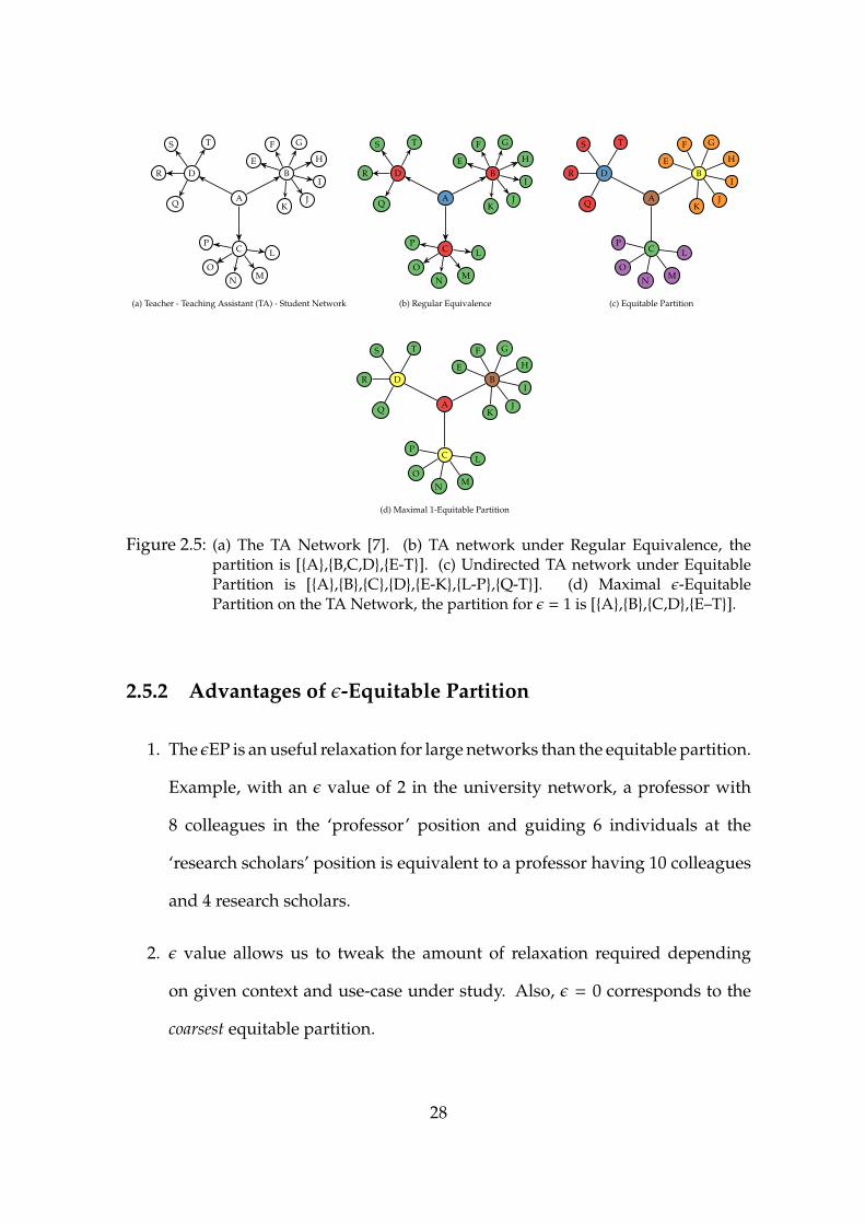
We use the Teacher-TA-Student example network from [7] to show the positions

captured by various equivalence relations. Figure 2.5 (a) shows the TA Network,

the network depicts an example classroom scenario in a department of an university

having three positions, wherein the node A is a teacher who teaches a class of 16

students (nodes E – T), A is assisted by 3 teaching assistants B, C and D, each of

them assists a group of 7, 5 and 4 students respectively. Figure 2.5 (b) and (c) show

the partitions of the TA network under RE and EP respectively. RE successfully

captures three positions, which are teacher, TAs and the students. EP on the other

hand leads to a trivial partitioning with 7 positions, treating each of the TA and

their respective student groups separate from each other. For this example, SE also

leads to the same partitioning as that of EP. Finally, Figure 2.5 (d) shows the maximal

εEP for an ε value of 1. The partition has 4 positions namely a teachers position

(block {A}), a students position (block {E–T}) and two TAs positions (blocks {B}

and {C,D}). Here, one might argue that the logical TAs position is split into two

positions, but interestingly on an intuitive thought we may counter argue that

the teaching assistant B was relatively overloaded than his counterparts C and

D. Hence, the ε-equitable partitioning of a graph corresponds to more intuitive

notions by considering the number of connections one has to the other positions

in the network.

27

A

BD

C L

MNO

P

I

J

GF

E

K

H

Q

R

S T

(a) Teacher - Teaching Assistant (TA) - Student Network

A

BD

C L

MNO

P

I

J

GF

E

K

H

Q

R

S T

(b) Regular Equivalence

A

BD

C

I

J

GF

E

K

H

L

MNO

P

Q

R

S T

(c) Equitable Partition

A

BD

C

I

J

GF

E

K

H

L

MNO

P

Q

R

S T

(d) Maximal 1-Equitable Partition

Figure 2.5: (a) The TA Network [7]. (b) TA network under Regular Equivalence, thepartition is [{A},{B,C,D},{E-T}]. (c) Undirected TA network under EquitablePartition is [{A},{B},{C},{D},{E-K},{L-P},{Q-T}]. (d) Maximal ε-EquitablePartition on the TA Network, the partition for ε = 1 is [{A},{B},{C,D},{E–T}].

2.5.2 Advantages of ε-Equitable Partition

1. The εEP is an useful relaxation for large networks than the equitable partition.

Example, with an ε value of 2 in the university network, a professor with

8 colleagues in the ‘professor’ position and guiding 6 individuals at the

‘research scholars’ position is equivalent to a professor having 10 colleagues

and 4 research scholars.

2. ε value allows us to tweak the amount of relaxation required depending

on given context and use-case under study. Also, ε = 0 corresponds to the

coarsest equitable partition.

28

3. It is both strict and lenient than regular equivalence. Strict due to the fact that

εEP requires the number of connections between two nodes to a position to be

atmost ε apart for them to be called equivalent. RE on the other hand does not

care about the number of connections, it simply requires some connection.

Lenient than RE since, εEP considers a node having no connection to a

position as equivalent with another node having ε connections to the same

position.

4. εEP of a graph corresponds to intuitive notions.

2.5.3 Algorithm for finding an εEP from [1]

Kate ([1], Chapter 4) discusses 4 different algorithms to find the εEP of a graph.

Two of them find the maximal εEP, while the other two find the εEP for a given input

graph. We discuss the algorithm #4 briefly here, since it is used for experimental

validation of the proposed method. The pseudo code for Algorithm 4 (Chapter 4

[1]) is shown in Algorithm box 2. Input to this algorithm is (i) the graph, (ii) the

coarsest equitable partition of graph [5] and (iii) a value of ε. The cells in the input

equitable partition are arranged by ascending order of their block degrees¶. The

algorithm then computes the degree vector (Equation 2.6) for each of the vertices

in the graph G. The algorithm then tries to merge these cells by taking two

consecutive cells at a time. If the degree vectors of the member nodes from these

two cells are within ε distance of each other, they are merged into a single new

cell. For further merging, this new cell becomes the current cell, which is then

¶Cell or block degree of a cell of an equitable partition is the degree of the member nodes in thatblock.

29

compared with the next cell for a possible merger. If the merging fails, the next

cell becomes the current cell. The algorithm exits if no further merging of cells

is possible. Also, the degree vectors need to be updated whenever two cells are

merged. The time complexity of this algorithm to find εEP of a graph is O(n3).

Algorithm 2 Algorithm to find ε-equitable partition from [1]

1: Sort the input equitable partition according to ascending order of the degree ofthe blocks (degree of the block of an equitable partition is same as the degreeof the member nodes of that block)

2: for i = 0→ ε do3: merge all the blocks having degree = i into a single block and update the

partition by deleting the merged blocks and by adding the new block4: update the variable K according to the resulting partition5: end for6: for each node vi of the graph do7: calculate the degree vector

−−→deg(vi) . Equation 2.6

8: end for9: currentBlock = the first block in the ordered partition having degree > ε

10: for each block in the currentPartition do11: check if it can be merged with currentBlock without violating the ε criterion,

where ε = ε/2 . Please refer [1] for more details12: if condition in Step 11 is True then13: merge it with currentBlock and update the partition, K and the

degreeVectors14: else15: make the block as currentBlock and continue16: end if17: end for

30

CHAPTER 3

Scalable Positional Analysis: Fast and Scalable

Epsilon Equitable Partition Algorithm

In this chapter we propose and implement a new, scalable and distributed algorithm

based on the MapReduce methodology to find εEP of a graph. Empirical studies

on random power-law graphs show that our algorithm is highly scalable for sparse

graphs, thereby giving us the ability to study positional analysis on very large scale

networks. We also present the results of our algorithm on time evolving snapshots

of the facebook and flickr social graphs. Results show the importance of positional

analysis on large dynamic networks.

The rest of the chapter is organized as follows. In Section 3.2 we propose a new

algorithm with better heuristics for finding the ε-equitable partition of a graph.

Section 3.3 describes the Parallel εEP algorithm along with its implementation.

We present the scalability analysis, evaluation methodology, dataset details and

experimental results in Section 3.4.

3.1 Motivation

An ε-equitable partition (εEP) [1] is a notion of equivalence, which has many

advantages over the classical methods. εEP allows a leeway of ε in the number

of connections the actors at a same position can have with the actors at another

position. In the Indian movies dataset from IMDb, authors in [7] have shown that

actors who fall in the same cell of the partition, tend to have acted in similar kinds of

movies. Further, the authors also show that people who belong to a same position

of an εEP tend to evolve similarly. In large social networks, tagging people who

belong to the same position has potentially many advantages, both from business

and individual perspective, such as, position based targeted promotions, ability to

find anomalies, user churn prediction and personalised recommendations.

Though efficient graph partition refinement techniques and their application in

finding the regular equivalence of a graph are well studied in the graph theoretic

literature [8, 9], the application of these techniques for doing positional analysis

of very large social graphs and networks is so far unknown. In this work, we

propose a new algorithm to find the ε-equitable partition of a graph and focus on

scaling this algorithm. We have successfully validated our algorithm with detailed

studies on facebook social graph, highlighting the advantages of doing positional

analysis on time evolving social network graphs. We present few results on a

relatively large component of the flickr social network. Further more, the empirical

scalability analysis of the proposed new algorithm shows that the algorithm is

highly scalable for very large sparse graphs.

3.2 Fast ε-Equitable Partition

Our proposed new algorithm with better heuristics to find an ε-equitable partitioning

of a graph is given in Algorithm 4. The implementation of our Fast εEP algorithm

is directly based on the modification of McKay’s original algorithm [5] to find the

32

equitable partition of a graph, which iteratively refines an ordered partition until

it is equitable (Chapter 2, 2.3.4). The key idea in our algorithm is to allow splitting

a cell only when the degrees of the member nodes of a cell are more than ε apart.

To achieve that, we first modify the split procedure of Algorithm 1, such that, it

captures the definition of ε-equitable partition as defined by Equation 2.4. The new

split function is listed in Algorithm 3. The key modifications are listed as follows:

• The input coloured partition π to Algorithm 1 is the ordered unit partition

of G (i.e. all vertices belong to a single cell). The initial ordering of the unit

partition is done by sorting the contents of the partition based on the output

of function f , considering the unit partition as the active cell.

• An additional input parameter ε is passed to the algorithm.

• The default split procedure on line 7 of Algorithm 1 is replaced by the split

procedure from Algorithm 3.

Key difference between the split procedure of Algorithm 1 (Chapter 2, 2.3.4)

and split from Algorithm 3 is the fact that the latter “splits” each cell of partition π

only when their sorted keys as assigned by the function f (Equation 2.3), w.r.t. the

current active cell are more than ε apart.

The algorithm for finding ε-equitable partition of G is given in Algorithm 4.

3.2.1 Description of Fast εEP Algorithm

The algorithm starts with the unit partition of the graph G and the current active

cell ca having the entire vertex set V. It then computes the function f (line 5,

33

Algorithm 3 Function split for finding ε-equitable partitionInput: epsilon ε, function f , partition πOutput: split partition πs

1: idx = 0 . index variable for πs

2: for each currentCell in π do3: sortedCell = sort(currentCell) using f as the comparison key . i.e. if

f (u) < f (v) then u appears before v in sortedCell4: currentDegree = f (sortedCell[0])5: for each vertex in sortedCell do6: if ( f (vertex) − currentDegree) ≤ ε then7: Add vertex to cell πs[idx]8: else9: currentDegree = f (vertex)

10: idx = idx + 111: Add vertex to cell πs[idx]12: end if13: end for14: idx = idx + 115: end for16: return πs

Algorithm 4 Fast ε-Equitable PartitionInput: graph G, ordered unit partition π, epsilon εOutput: ε-equitable partition π

1: active = indices(π)2: while (active , φ) do3: idx = min(active)4: active = active r {idx}5: f (u) = deg(u, π[idx]) ∀u ∈ V . f : V→N6: π′ = split(π, f , ε) . Algorithm 37: active = active∪ [ordered indices of newly split cells fromπ′, while replacing

(in place) the indices from π which were split]8: π = π′

9: end while10: return π

34

Algorithm 4) for each of the vertices of the graph. The algorithm then calls the

split function (Algorithm 3). The split function takes each cell from the partitionπ

and sorts the member vertices of these cells using the function f as the comparison

key (Equation 2.3). Once a cell is sorted, a linear pass through the member vertices

of the cell is done to check if any two consecutive vertices violate the ε criteria.

In case of violation of the ε condition, the function splits the cell and updates the

partition π and the active list accordingly. The algorithm exits either when the

active list is empty or when π becomes a discrete partition, i.e., all cells in π are

singletons.

Explanation: The algorithm starts with “splitting” the ordered unit partition wherever

the ε property to “itself ” is violated and updates the partition π accordingly. In the

second iteration, second cell of π is marked active, the function f is then populated

w.r.t. this cell. Again, the algorithm “splits” each of the cells inπwhich violate the ε

criteria (Eq. 2.4) to the second cell, updates π and so on. The algorithm terminates

when no further splits of π are possible. At each iteration of the algorithm, the

ordered∗ property of the partition is preserved, this is achieved by updating the list

of active indices in-place. Example,

let π = {c1, c2, ..., ci, ..., cn} be a partition at some intermediate iteration of Algorithm

4 and the current active list = indices[c2, c3, ..., ci, ..., cn]. Now suppose, the new

partition π′ generated by the procedure split (line 6, Algorithm 4) is,

π′ = {c1, c2, ..., ci−1, s1, s2, ..., s j, ci+1, ..., cn}, i.e. cell ci ofπ is “split” to cells (s1, s2, ..., s j) in

π′, then new active list = indices[c2, c3, ..., ci−1, s1, s2, ..., s j, ci+1, ..., cn] (line 7, Algorithm

4). The dry run of the Fast εEP Algorithm 4 on the example TA Network of Figure

∗Mathematically, the definition of a partition doesn’t force an ordering on the member cells/blocks.We abuse the cell index preserving partition as an ordered partition.

35

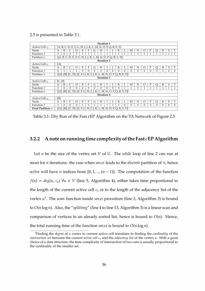
2.5 is presented in Table 3.1.

Iteration 1Active Cell ca [A, B, C, D, E, F, G, H, I, J, K, L, M, N, O, P, Q, R, S, T]Node A B C D E F G H I J K L M N O P Q R S TFunction f 3 8 6 5 1 1 1 1 1 1 1 1 1 1 1 1 1 1 1 1Partition π {[A, B, C, D, E, F, G, H, I, J, K, L, M, N, O, P, Q, R, S, T]}

Iteration 2Active Cell ca [A]Node A B C D E F G H I J K L M N O P Q R S TFunction f 0 1 1 1 0 0 0 0 0 0 0 0 0 0 0 0 0 0 0 0Partition π {[A], [B], [C, D], [E, F, G, H, I, J, K, L, M, N, O, P, Q, R, S, T]}

Iteration 3Active Cell ca [C, D]Node A B C D E F G H I J K L M N O P Q R S TFunction f 2 0 0 0 0 0 0 0 0 0 0 1 1 1 1 1 1 1 1 1Partition π {[A], [B], [C, D], [E, F, G, H, I, J, K, L, M, N, O, P, Q, R, S, T]}

Iteration 4Active Cell ca [B]Node A B C D E F G H I J K L M N O P Q R S TFunction f 1 0 0 0 1 1 1 1 1 1 1 0 0 0 0 0 0 0 0 0Final Partition π {[A], [B], [C, D], [E, F, G, H, I, J, K, L, M, N, O, P, Q, R, S, T]}

Table 3.1: Dry Run of the Fast εEP Algorithm on the TA Network of Figure 2.5

3.2.2 A note on running time complexity of the Fast εEP Algorithm

Let n be the size of the vertex set V of G. The while loop of line 2 can run at

most for n iterations: the case when split leads to the discrete partition of π, hence

active will have n indices from [0, 1, ..., (n − 1)]. The computation of the function

f (u) = deg(u, ca) ∀u ∈ V (line 5, Algorithm 4), either takes time proportional to

the length of the current active cell ca or to the length of the adjacency list of the

vertex u†. The sort function inside split procedure (line 3, Algorithm 3) is bound

to O(n log n). Also, the “splitting” (line 4 to line 13, Algorithm 3) is a linear scan and

comparison of vertices in an already sorted list, hence is bound to O(n). Hence,

the total running time of the function split is bound to O(n log n).

†Finding the degree of a vertex to current active cell translates to finding the cardinality of theintersection set between the current active cell ca and the adjacency list of the vertex u. With a goodchoice of a data structure, the time complexity of intersection of two sets is usually proportional tothe cardinality of the smaller set.

36

The maximum cardinality of the current active cell ca can at most be n. Further,

for dense undirected simple graph, the maximum cardinality of the adjacency list of

any vertex can also at most be (n − 1). Therefore for n vertices, line 5 of Algorithm

4 performs in O(n2). For sparse graphs, the cardinality of the entire edge set is of

the order of n, hence line 5 of algorithm 4 performs in the order O(n).

Therefore, the total running time complexity of the proposed Fast ε-Equitable

Partitioning algorithm is O(n3) for dense graphs and O(n2 log n) for sparse graphs.

In reality this would be quite less, since subsequent splits would only reduce the

cardinality of the current active cell ca. Which implies that we can safely assume

that the cardinality of set ca will be less than the cardinality of the adjacency list of

the vertices of the graph. This analysis is only for the serial algorithm. Empirical

scalability analysis on random power-law graphs shows that our parallel algorithm

(Section 3.3, Algorithm 5) is an order faster in time for sparse graphs.

3.3 Scalable and Distributed ε-Equitable Partition

This section describes the parallel implementation of the Fast ε-EP Algorithm 4 by

the MapReduce methodology.

3.3.1 Overview of MapReduce

MapReduce (MR) [10] is a programming model to process large amounts of data

using distributed computing nodes and algorithms that can be parallelized based

on this paradigm. The MR paradigm is based on two main steps:

37

• Map step - Master node divides the input into smaller sub-problems and

distributes amongst worker nodes in the cluster. Workers process the smaller

problem and send back the result to the master node.

• Reduce step - The master combines the individual results from each of the

worker nodes to generate the output.

3.3.2 Logical/Programming View of the MR Paradigm

Both the Map and Reduce procedures are defined w.r.t. as set of (key,value) pair.

The Map function is applied in parallel to each of the input record pairs at the

worker nodes, which in turn generate an intermediate (key,value) pair. All these

intermediate records are sent back to the master node, which groups the records

for each intermediate key and then passes it to the reduce function.

The Reduce function accepts an intermediate key and a set of values for that

key. It merges together these values to form a (possibly) smaller set of values. The

return of these reduce functions is collected as the result list.

Mathematically,

• Map(k1, v1)→ list(k2, v2)

• Reduce(k2, list(v2))→ list(v2)

The input (key, value) pairs are drawn from a different domain than the output

(key, value) pairs. Furthermore, the intermediate (key, value) pairs are from the

same domain as the output (key, value) pairs. Thus, the MR paradigm transforms

input (key, value) pairs into list of values.

38

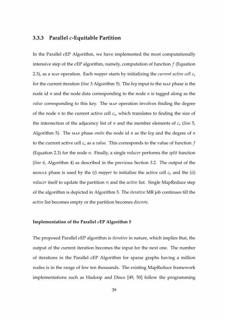
3.3.3 Parallel ε-Equitable Partition

In the Parallel εEP Algorithm, we have implemented the most computationally

intensive step of the εEP algorithm, namely, computation of function f (Equation

2.3), as a map operation. Each mapper starts by initializing the current active cell ca

for the current iteration (line 3 Algorithm 5). The key input to the map phase is the

node id n and the node data corresponding to the node n is tagged along as the

value corresponding to this key. The map operation involves finding the degree

of the node n to the current active cell ca, which translates to finding the size of

the intersection of the adjacency list of n and the member elements of ca (line 5,

Algorithm 5). The map phase emits the node id n as the key and the degree of n

to the current active cell ca as a value. This corresponds to the value of function f

(Equation 2.3) for the node n. Finally, a single reducer performs the split function

(line 6, Algorithm 4) as described in the previous Section 3.2. The output of the

reduce phase is used by the (i) mapper to initialize the active cell ca and the (ii)

reducer itself to update the partition π and the active list. Single MapReduce step

of the algorithm is depicted in Algorithm 5. The iterative MR job continues till the

active list becomes empty or the partition becomes discrete.

Implementation of the Parallel εEP Algorithm 5

The proposed Parallel εEP algorithm is iterative in nature, which implies that, the

output of the current iteration becomes the input for the next one. The number

of iterations in the Parallel εEP Algorithm for sparse graphs having a million

nodes is in the range of few ten thousands. The existing MapReduce framework

implementations such as Hadoop and Disco [49, 50] follow the programming

39

Algorithm 5 MapReduce step of the Parallel ε-Equitable Partition

1: class Mapper2: method initialize()3: ca ←Current Active Cell . active[0]4: method map(id n, vertex N)5: d← |N.AdjacencyList ∩ ca| . d corresponds to the value of function f (n),

Equation 2.36: emit(id n, value d)

1: class Reducer . Single Reducer2: method reduce()3: split(π, f , ε) . Algorithm 34: update(active) . Algorithm 4, line 75: update(π)

model and its architecture from the original MapReduce paradigm [10]. Hence,

these implementations focus more on data reliability and fault tolerance guarantees

in large cluster environments. This reliability and fault tolerance is usually

associated with high data copy and job setup overhead costs. Although these

features are suited for programs with a singlemap& a single reduce operation, they

introduce high job setup overhead times across the iterative MR steps [51, 52, 53].

To circumvent this, we implemented a bare minimum MapReduce framework

using open source tools GNU Parallel and rsync [54, 55]. We used GNU Parallel to

trigger parallel map and reduce jobs on the cluster, rsync was used for data copy

across the cluster nodes. We were able to achieve job setup overhead time in the

range of few milliseconds using the custom framework, as opposed to ˜30 − 45

seconds for Hadoop on a 10 node cluster isolated over a Gigabit Ethernet switch.

Conceptual and detailed overview of our Lightweight MapReduce Framework

implementation is depicted in Figure 3.1. We intelligently sharded the input

graph data across the distributed computing nodes. The node data partitioning

is performed based on the number of nodes n in the input graph and the number

40

of cores p available for computation; the methodology is depicted in Figure 3.1(b).

The node partition splits the input graph into nearly equal sized vertex groups for

processing on each of the available cores, we cache the vertex data for each of

these groups on the corresponding compute nodes. This is conceptually similar to

the user control on data persistence and data partitioning in the Resilient Distributed

Datasets in the Spark MapReduce framework [53, 56]; though our implementation

was inspired independently of the Spark framework and realized before that. This

helped us achieve locality in reading the input graph. Execution time empirical

studies on random power-law graphs for the proposed Algorithm 5 are presented

in Section 3.4.5.

3.4 Experimental Evaluation

In this section we first present the results of our Fast εEP algorithm on a small

example toy network. Later we briefly talk about the datasets used for evaluating

our proposed algorithm. We also discuss the evaluation methodology and present

our results. Finally, we do the scalability analysis of the proposed Parallel εEP

algorithm.

3.4.1 Evaluation on an Example Toy Network

We performed static analysis of the ε-equitable partition algorithm on the TA

Network using the εEP Algorithm from [7] and the proposed Fast εEP Algorithm

4 for ε = 1. The TA Network depicts an University classroom scenario in which

the node A signifies the position professor, the nodes B,C and D represent the

41

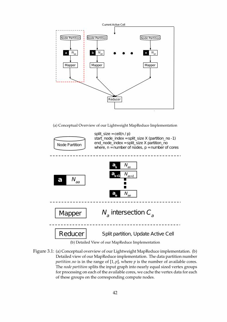
Node Partition

a Naa

Mapper

b Nab

Mapper

n Nan

Mapper

Reducer

Current Active Cell

Node Partition Node Partition

(a) Conceptual Overview of our Lightweight MapReduce Implementation

as Nas

Mapper

Node Partition

split_size =ceil(n / p)start_node_index =split_size X (partition_no -1)end_node_index =split_size X partition_nowhere, n =number of nodes, p =number of cores

a Naa

as+1 Nas+1...ae Nae

Na intersectionCa

Reducer Split partition, Update Active Cell

(b) Detailed View of our MapReduce Implementation

Figure 3.1: (a) Conceptual overview of our Lightweight MapReduce implementation. (b)Detailed view of our MapReduce implementation. The data partition numberpartition no is in the range of [1, p], where p is the number of available cores.The node partition splits the input graph into nearly equal sized vertex groupsfor processing on each of the available cores, we cache the vertex data for eachof these groups on the corresponding compute nodes.

42

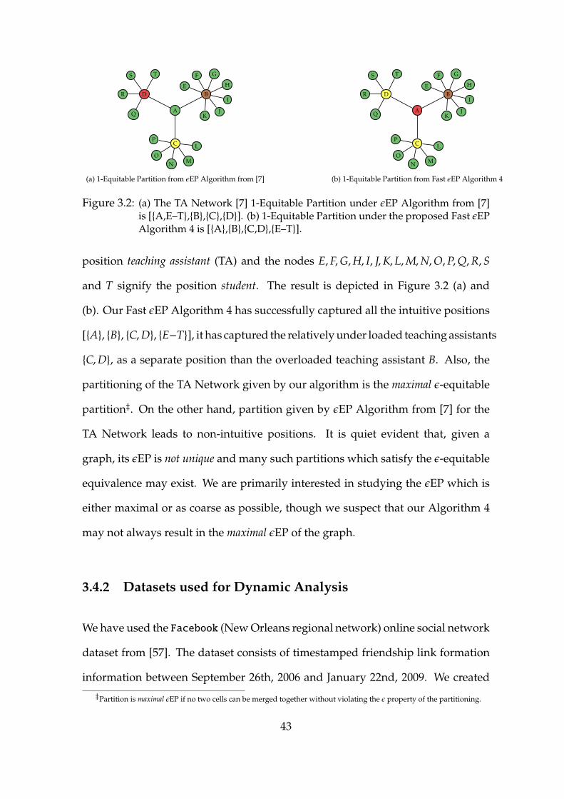
A

BD

C L

MNO

P

I

J

GF

E

K

H

Q

R

S T

(a) 1-Equitable Partition from εEP Algorithm from [7]

A

BD

C

I

J

GF

E

K

H

L

MNO

P

Q

R

S T

(b) 1-Equitable Partition from Fast εEP Algorithm 4

Figure 3.2: (a) The TA Network [7] 1-Equitable Partition under εEP Algorithm from [7]is [{A,E–T},{B},{C},{D}]. (b) 1-Equitable Partition under the proposed Fast εEPAlgorithm 4 is [{A},{B},{C,D},{E–T}].

position teaching assistant (TA) and the nodes E,F,G,H, I, J,K,L,M,N,O,P,Q,R,S

and T signify the position student. The result is depicted in Figure 3.2 (a) and

(b). Our Fast εEP Algorithm 4 has successfully captured all the intuitive positions

[{A}, {B}, {C,D}, {E−T}], it has captured the relatively under loaded teaching assistants

{C,D}, as a separate position than the overloaded teaching assistant B. Also, the

partitioning of the TA Network given by our algorithm is the maximal ε-equitable

partition‡. On the other hand, partition given by εEP Algorithm from [7] for the

TA Network leads to non-intuitive positions. It is quiet evident that, given a

graph, its εEP is not unique and many such partitions which satisfy the ε-equitable

equivalence may exist. We are primarily interested in studying the εEP which is

either maximal or as coarse as possible, though we suspect that our Algorithm 4

may not always result in the maximal εEP of the graph.

3.4.2 Datasets used for Dynamic Analysis

We have used the Facebook (New Orleans regional network) online social network

dataset from [57]. The dataset consists of timestamped friendship link formation

information between September 26th, 2006 and January 22nd, 2009. We created‡Partition is maximal εEP if no two cells can be merged together without violating the ε property of the partitioning.

43

three time evolving graph snapshots for the facebook network, the base network

consists of all the links formed between September 26th, 2006 and June 22nd 2007.

The remaining two graphs are created such that, the graph at evolved point of time

t + δ(t) has the graph at time t, along with the new vertices and edges that were

added to the graph between time t and time t + δ(t), with δ(t) being 290 days. We

refer to these three datasets as Facebook graphs G1, G2 and G3 respectively. Table

3.2 tabulates the dataset properties. The degree distribution for the Facebook

graph G3 is shown in Figure 3.3.

100 101 102 103

node degree (d)

100

101

102

103

104

# n

odes

with

deg

ree ≥

d

Degree Distribution of Facebook Graph G3

Figure 3.3: Degree Distribution for Facebook graph G3.

The second dataset that we used is the Flickr social network dataset from

[58], which consists of a total of 104 days (November 2nd - December 3rd, 2006,

and February 3rd - May 18th, 2007) of crawl data. This dataset consists of the

timestamped link formation information among nodes. Since the nature of contact

links in Flickr are directional in nature, we create an undirected dataset as described

next. For each outgoing link from user a→ b, if user b reciprocates the link b→ a,

44

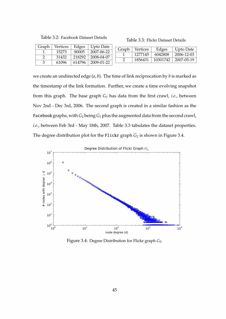
Table 3.2: Facebook Dataset Details

Graph Vertices Edges Upto Date1 15273 80005 2007-06-222 31432 218292 2008-04-073 61096 614796 2009-01-22

Table 3.3: Flickr Dataset Details

Graph Vertices Edges Upto Date1 1277145 6042808 2006-12-032 1856431 10301742 2007-05-19

we create an undirected edge (a, b). The time of link reciprocation by b is marked as

the timestamp of the link formation. Further, we create a time evolving snapshot

from this graph. The base graph G1 has data from the first crawl, i.e., between

Nov 2nd - Dec 3rd, 2006. The second graph is created in a similar fashion as the

Facebookgraphs, with G2 being G1 plus the augmented data from the second crawl,

i.e., between Feb 3rd - May 18th, 2007. Table 3.3 tabulates the dataset properties.

The degree distribution plot for the Flickr graph G2 is shown in Figure 3.4.

100 101 102 103 104

node degree (d)

100

101

102

103

104

105

106

107

# n

odes

with

deg

ree ≥

d

Degree Distribution of Flickr Graph G2

Figure 3.4: Degree Distribution for Flickr graph G2.

45

3.4.3 Evaluation Methodology

We are primarily interested in studying the effect of PA on dynamic social networks

and to characterize what role PA plays in the co-evolution of nodes in the networks.

Given, a social network graph Gt at time t and its evolved network graph Gt+δt,

our algorithm would return an ε-equitable partitioning πt for Gt and πt+δt for Gt+δt.

The methodology used to evaluate our proposed εEP algorithm is as follows.

i. Partition Similarity: We find the fraction of actors who share the same

position across the partitions πt and πt+δt using Equation 3.1. We introduce

a notion which assigns a value of 1 for exact partition match and 0 for a

completely different partitioning. The size of the discrete partition of πt,

denoted by N in the equation captures the deviation of a partition from

the discrete partition of the network. The new nodes in Gt+δt, which are

not present in Gt are dropped off from πt+δt before computing the partition

similarity score.

sim(πt, πt+δt) =12

[(N − |πt ∩ πt+δt|

N − |πt|

)+

(N − |πt ∩ πt+δt|

N − |πt+δt|

)](3.1)

where, N is the size of the discrete partition ofπt. The quantity |πt∩πt+δt| is the

size of the partition obtained by doing cell-wise intersection among the cells

of πt and πt+δt. In equation 3.1, if the number of actors who share positions

across πt and πt+δt is large, the value of |πt ∩ πt+δt| will be almost equal to

the size of either πt or πt+δt. Hence, the resulting partition similarity score

will be close to 1. On the other hand, if the overlap of actors between πt and

πt+δt is very small, |πt ∩ πt+δt|will be a large number, resulting in a similarity

46

score close to 0. The terms in the denominator of the equation essentially

provide a normalization w.r.t. the size of partitions πt and πt+δt. The value

of sim(πt, πt+δt) given by Equation 3.1 is always between [0, 1]. We provide a

detailed note on the partition similarity and its computation in Appendix A.

ii. Graph theoretic network centric properties: Given co-evolving vertex pairs

(a, b) which occupy the same position in the partition πt, we study the

evolution of network centric properties corresponding to the vertex pairs

in the time evolved graph Gt+δt. We study the following properties which are

widely used for characterizing the graph structure:

• Betweenness centrality of a node v is the number of shortest paths across

all the node pairs that pass through v. This signifies the importance of

a node, for routing, information diffusion, etc.

• Degree centrality of a node is the number of nodes it is connected to in

a graph. It quantifies the importance of a node w.r.t. the number of

connections a node has.

• Counting the number of triangles a node is part of, is an elementary

step required to find the clustering co-efficient of a node in a graph.

Clustering co-efficient of a node signifies how strongly-knit a node is

with its neighbourhood. There is a scalable algorithm to count the

number of triangles in a graph [59].

• Shapley value centrality corresponds to a game theoretic notion of centrality.

This models the importance of a node in information diffusion [60], it

is also efficiently computable for large graphs. An actor has a higher

shapley value centrality when its degree is higher in comparison to the

47

degree of its neighbours. The notion captures the summation of inverse

degrees of an actor’s neighbourhood.

We evaluate the co-evolution of nodes in various positional analysis methods

using these four network centric properties as follows. For each pair of nodes

(a, b) which occupy same position in a partition, we compute the difference

(at − bt). Where, at and bt correspond to the score of either of these four

properties described previously. For the same pair of nodes, we also compute

the difference (at+δt−bt+δt). The scores at+δt and bt+δt correspond to the property

score at time t + δt. Finally, we take an absolute value of the difference of

these two quantities, i.e., |(at − bt)− (at+δt − bt+δt)|. A low value of this quantity

therefore signifies that for a co-evolving node pair (a, b) at time t, the network

centric property of node a and b at time t+δt have also evolved similarly. Note

that, when there is no activity, then the role continues to be the same - hence

from a co-evolution point of view, the nodes have co-evolved. Also, since we

are not partitioning based on the centrality scores, hence our comparisons

are across timestamps.

A note on choice of ε We vary ε between ε = 1 to average degree of the network.

The intuition for choosing maximum ε value as the average degree of the network

is as follows: By choosing an ε = x, all the nodes with a degree ≤ x would belong to

a same position under the ε-equitable partition (εEP). This essentially implies that

nodes with a degree of x are partitioned trivially for ε = x by the definition an εEP.

Therefore, we don’t use ε values greater than the average network degree.

48

0 50000 100000 150000 2000000

20

40

60

80

100C

ount

(pe

rcen

tage

)

DEGREEEEP0EEP1EEP2EEP4EEP8

(a) Difference of Betweenness Centrality

0.00000 0.00025 0.00050 0.00075 0.00100 0.00125 0.00150 0.001750

20

40

60

80

100

Cou

nt (

perc

enta

ge)

DEGREEEEP0EEP1EEP2EEP4EEP8

(b) Difference of Normalized Degree Centrality

Figure 3.5: Co-evolving Node Pairs for Facebook Graph G1 → G2. (a) Difference ofBetweenness Centrality. (b) Difference of Normalized Degree Centrality.

49

0.0 0.5 1.0 1.5 2.00

20

40

60

80

100

Cou

nt (

perc

enta

ge)

DEGREEEEP0EEP1EEP2EEP4EEP8

(c) Difference of Shapley Value Centrality

0 50 100 150 2000

20

40

60

80

100

Coun

t (pe

rcen

tage

)

DEGREEEEP0EEP1EEP2EEP4EEP8

(d) Difference of Triangles

Figure 3.5: Co-evolving Node Pairs for Facebook Graph G1 → G2. (c) Difference ofShapley Value Centrality. (d) Difference of Triangles.

50

0 100000 200000 300000 4000000

20

40

60

80

100C

ount

(pe

rcen

tage

)

DEGREEEEP0EEP1EEP2EEP4EEP8

(a) Difference of Betweenness Centrality

0.00000 0.00025 0.00050 0.00075 0.00100 0.00125 0.00150 0.001750

20

40

60

80

100

Cou

nt (

perc

enta

ge)

DEGREEEEP0EEP1EEP2EEP4EEP8

(b) Difference of Normalized Degree Centrality

Figure 3.6: Co-evolving Node Pairs for Facebook Graph G2 → G3. (a) Difference ofBetweenness Centrality. (b) Difference of Normalized Degree Centrality.

51

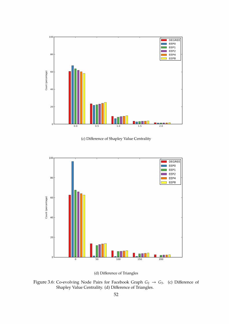
0.0 0.5 1.0 1.5 2.00

20

40

60

80

100

Coun

t (pe

rcen

tage

)

DEGREEEEP0EEP1EEP2EEP4EEP8

(c) Difference of Shapley Value Centrality

0 50 100 150 2000

20

40

60

80

100

Coun

t (pe

rcen

tage

)

DEGREEEEP0EEP1EEP2EEP4EEP8

(d) Difference of Triangles

Figure 3.6: Co-evolving Node Pairs for Facebook Graph G2 → G3. (c) Difference ofShapley Value Centrality. (d) Difference of Triangles.

52

0 100000 200000 300000 4000000

20

40

60

80

100C

ount

(pe

rcen

tage

)

DEGREEEEP0EEP1EEP2EEP4EEP8

(a) Difference of Betweenness Centrality

0.00000 0.00025 0.00050 0.00075 0.00100 0.00125 0.00150 0.001750

20

40

60

80

100

Cou

nt (

perc

enta

ge)

DEGREEEEP0EEP1EEP2EEP4EEP8

(b) Difference of Normalized Degree Centrality

Figure 3.7: Co-evolving Node Pairs for Facebook Graph G1 → G3. (a) Difference ofBetweenness Centrality. (b) Difference of Normalized Degree Centrality.

53

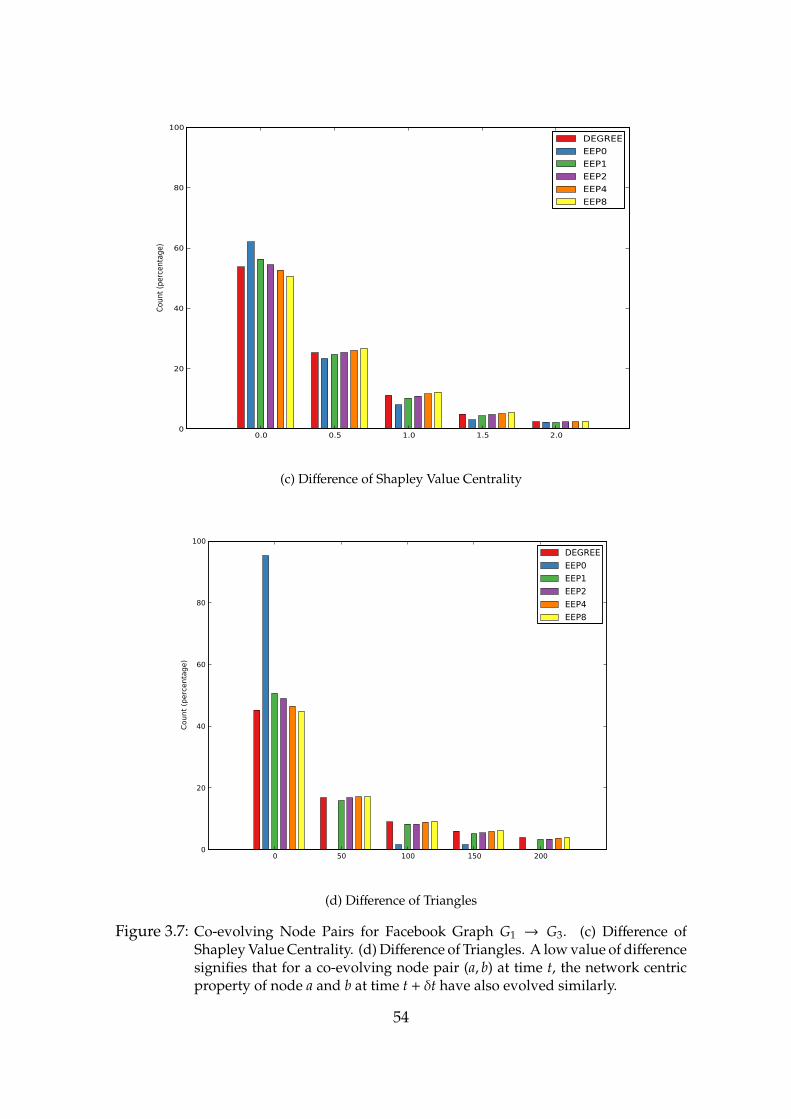
0.0 0.5 1.0 1.5 2.00

20

40

60

80

100

Coun

t (pe

rcen

tage

)

DEGREEEEP0EEP1EEP2EEP4EEP8

(c) Difference of Shapley Value Centrality

0 50 100 150 2000

20

40

60

80

100

Coun

t (pe

rcen

tage

)

DEGREEEEP0EEP1EEP2EEP4EEP8

(d) Difference of Triangles

Figure 3.7: Co-evolving Node Pairs for Facebook Graph G1 → G3. (c) Difference ofShapley Value Centrality. (d) Difference of Triangles. A low value of differencesignifies that for a co-evolving node pair (a, b) at time t, the network centricproperty of node a and b at time t + δt have also evolved similarly.

54

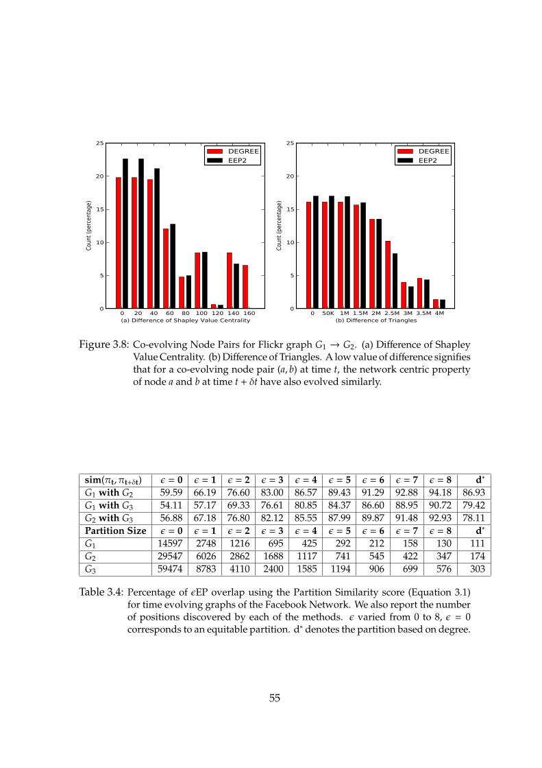
0 20 40 60 80 100 120 140 160(a) Difference of Shapley Value Centrality

0

5

10

15

20

25

Coun

t (pe

rcent

age)

DEGREEEEP2

0 50K 1M 1.5M 2M 2.5M 3M 3.5M 4M(b) Difference of Triangles

0

5

10

15

20

25

Coun

t (pe

rcent

age)

DEGREEEEP2

Figure 3.8: Co-evolving Node Pairs for Flickr graph G1 → G2. (a) Difference of ShapleyValue Centrality. (b) Difference of Triangles. A low value of difference signifiesthat for a co-evolving node pair (a, b) at time t, the network centric propertyof node a and b at time t + δt have also evolved similarly.

sim(πt, πt+δt) ε = 0 ε = 1 ε = 2 ε = 3 ε = 4 ε = 5 ε = 6 ε = 7 ε = 8 d∗

G1 with G2 59.59 66.19 76.60 83.00 86.57 89.43 91.29 92.88 94.18 86.93G1 with G3 54.11 57.17 69.33 76.61 80.85 84.37 86.60 88.95 90.72 79.42G2 with G3 56.88 67.18 76.80 82.12 85.55 87.99 89.87 91.48 92.93 78.11Partition Size ε = 0 ε = 1 ε = 2 ε = 3 ε = 4 ε = 5 ε = 6 ε = 7 ε = 8 d∗

G1 14597 2748 1216 695 425 292 212 158 130 111G2 29547 6026 2862 1688 1117 741 545 422 347 174G3 59474 8783 4110 2400 1585 1194 906 699 576 303

Table 3.4: Percentage of εEP overlap using the Partition Similarity score (Equation 3.1)for time evolving graphs of the Facebook Network. We also report the numberof positions discovered by each of the methods. ε varied from 0 to 8, ε = 0corresponds to an equitable partition. d∗ denotes the partition based on degree.

55

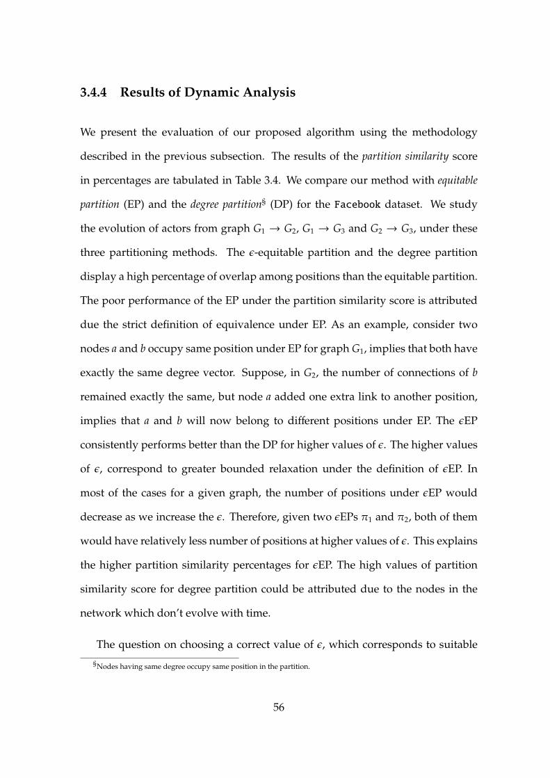
3.4.4 Results of Dynamic Analysis

We present the evaluation of our proposed algorithm using the methodology

described in the previous subsection. The results of the partition similarity score

in percentages are tabulated in Table 3.4. We compare our method with equitable

partition (EP) and the degree partition§ (DP) for the Facebook dataset. We study

the evolution of actors from graph G1 → G2, G1 → G3 and G2 → G3, under these

three partitioning methods. The ε-equitable partition and the degree partition

display a high percentage of overlap among positions than the equitable partition.

The poor performance of the EP under the partition similarity score is attributed

due the strict definition of equivalence under EP. As an example, consider two

nodes a and b occupy same position under EP for graph G1, implies that both have

exactly the same degree vector. Suppose, in G2, the number of connections of b

remained exactly the same, but node a added one extra link to another position,

implies that a and b will now belong to different positions under EP. The εEP

consistently performs better than the DP for higher values of ε. The higher values

of ε, correspond to greater bounded relaxation under the definition of εEP. In

most of the cases for a given graph, the number of positions under εEP would

decrease as we increase the ε. Therefore, given two εEPs π1 and π2, both of them

would have relatively less number of positions at higher values of ε. This explains

the higher partition similarity percentages for εEP. The high values of partition

similarity score for degree partition could be attributed due to the nodes in the

network which don’t evolve with time.

The question on choosing a correct value of ε, which corresponds to suitable

§Nodes having same degree occupy same position in the partition.

56

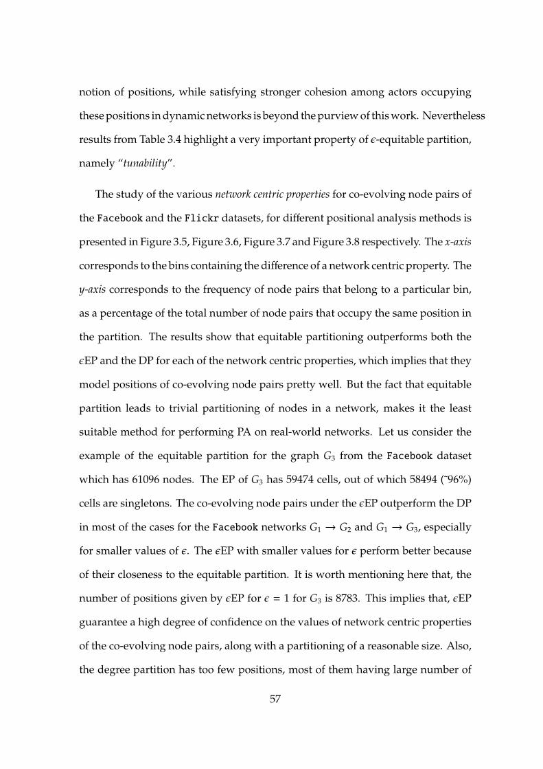
notion of positions, while satisfying stronger cohesion among actors occupying

these positions in dynamic networks is beyond the purview of this work. Nevertheless

results from Table 3.4 highlight a very important property of ε-equitable partition,

namely “tunability”.

The study of the various network centric properties for co-evolving node pairs of

the Facebook and the Flickr datasets, for different positional analysis methods is

presented in Figure 3.5, Figure 3.6, Figure 3.7 and Figure 3.8 respectively. The x-axis

corresponds to the bins containing the difference of a network centric property. The

y-axis corresponds to the frequency of node pairs that belong to a particular bin,

as a percentage of the total number of node pairs that occupy the same position in

the partition. The results show that equitable partitioning outperforms both the

εEP and the DP for each of the network centric properties, which implies that they

model positions of co-evolving node pairs pretty well. But the fact that equitable

partition leads to trivial partitioning of nodes in a network, makes it the least

suitable method for performing PA on real-world networks. Let us consider the

example of the equitable partition for the graph G3 from the Facebook dataset

which has 61096 nodes. The EP of G3 has 59474 cells, out of which 58494 (˜96%)

cells are singletons. The co-evolving node pairs under the εEP outperform the DP

in most of the cases for the Facebook networks G1 → G2 and G1 → G3, especially

for smaller values of ε. The εEP with smaller values for ε perform better because

of their closeness to the equitable partition. It is worth mentioning here that, the

number of positions given by εEP for ε = 1 for G3 is 8783. This implies that, εEP

guarantee a high degree of confidence on the values of network centric properties

of the co-evolving node pairs, along with a partitioning of a reasonable size. Also,

the degree partition has too few positions, most of them having large number of

57

nodes. The distribution of position sizes and their respective counts for each of

these methods is shown in Figure 3.9.

The Flickr dataset results in Figure 3.8 also follow a similar trend, the εEP

partition performs better than the DP. The percentage counts of both the properties

is more spread out across initial few bins for the Flickr dataset. The εEP for

ε = 2 has higher percentage counts for co-evolving node pairs in the bins, which

correspond to smaller difference values, whereas, the co-evolving node pairs from

the DP have relatively lower percentage counts in the bins closer to a difference

of zero and high percentage of nodes towards the tail end of the x-axis, especially,

for the shapley value centrality, which is not desirable. Also, the degree based

partition has very few positions. Therefore, εEP is a consistent performer, both

from the perspective of node co-evolution characteristics and number of positions

it gives.

58

0 2 4 6 8 10 12 14 16 18 20 22 24 26 28 30 32 34 36 38 40 42 44 46 ≥48Number of Actors at a Position

0

20

40

60

80

100

Freq

uenc

y

Distribution of Position Sizes under Degree Partition for Facebook Graph G3 Network

Degree

(a) Position Size Distribution for Degree Partition

0 2 4 6 8 10 12 14 16 18 20 22 24 26 28 30 32 34 36 38 40 42 44 46 ≥48Number of Actors at a Position

0

10000

20000

30000

40000

50000

60000

Freq

uenc

y

Distribution of Position Sizes under Equitable Partition for Facebook Graph G3 Network

Equitable

(b) Position Size Distribution for Equitable Partition

Figure 3.9: Position Size Distribution for Facebook Graph G3. (a) Degree Partition. (b)Equitable Partition. DP has problem of fewer positions having large numberof nodes. On the contrary, EP has too many positions, mostly singletons.

59

0 2 4 6 8 10 12 14 16 18 20 22 24 26 28 30 32 34 36 38 40 42 44 46 ≥48Number of Actors at a Position

0

1000

2000

3000

4000

5000

6000

7000

8000

Freq

uenc

y

Distribution of Position Sizes under EEP, ε = 1 for Facebook Graph G3 Network

EEP1

(c) Position Size Distribution for εEP, ε = 1

0 2 4 6 8 10 12 14 16 18 20 22 24 26 28 30 32 34 36 38 40 42 44 46 ≥48Number of Actors at a Position

0

500

1000

1500

2000

2500

3000

3500

Freq

uenc

y

Distribution of Position Sizes under EEP, ε = 2 for Facebook Graph G3 Network

EEP2

(d) Position Size Distribution for εEP, ε = 2

Figure 3.9: Position Size Distribution for Facebook Graph G3. (c) εEP, ε = 1. (d) εEP, ε = 2.

60

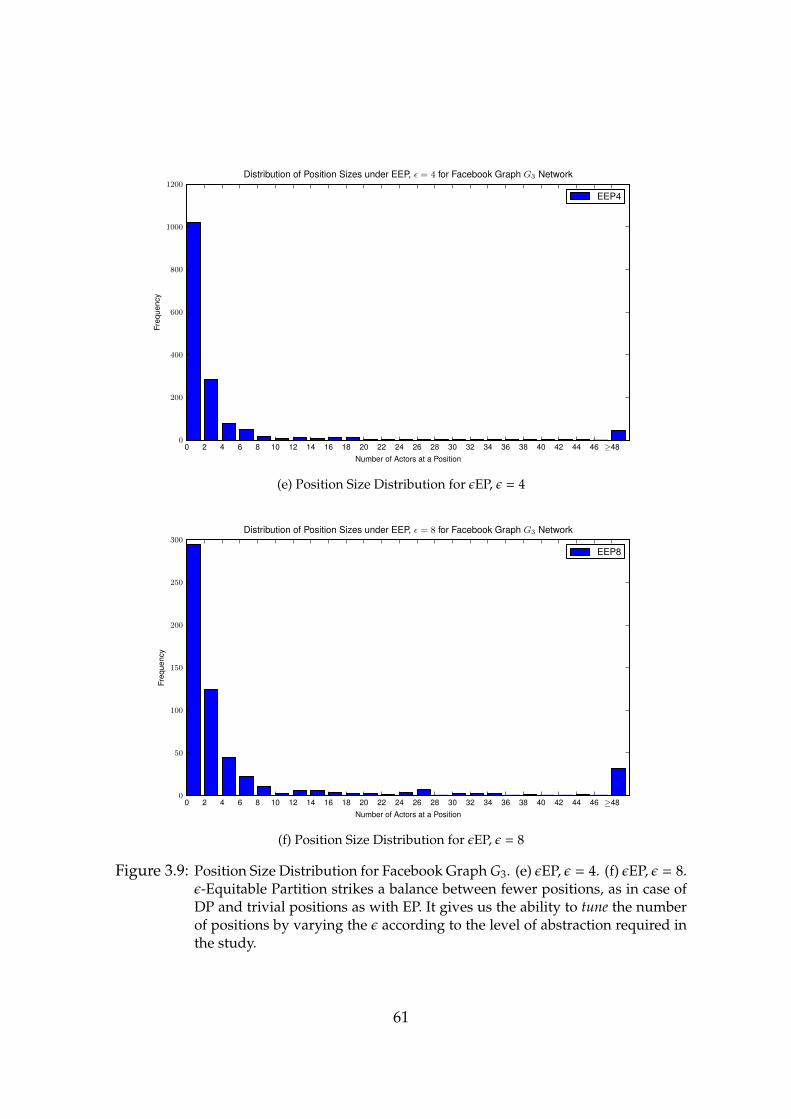
0 2 4 6 8 10 12 14 16 18 20 22 24 26 28 30 32 34 36 38 40 42 44 46 ≥48Number of Actors at a Position

0

200

400

600

800

1000

1200

Freq

uenc

y

Distribution of Position Sizes under EEP, ε = 4 for Facebook Graph G3 Network

EEP4

(e) Position Size Distribution for εEP, ε = 4

0 2 4 6 8 10 12 14 16 18 20 22 24 26 28 30 32 34 36 38 40 42 44 46 ≥48Number of Actors at a Position

0

50

100

150

200

250

300

Freq

uenc

y

Distribution of Position Sizes under EEP, ε = 8 for Facebook Graph G3 Network

EEP8

(f) Position Size Distribution for εEP, ε = 8

Figure 3.9: Position Size Distribution for Facebook Graph G3. (e) εEP, ε = 4. (f) εEP, ε = 8.ε-Equitable Partition strikes a balance between fewer positions, as in case ofDP and trivial positions as with EP. It gives us the ability to tune the numberof positions by varying the ε according to the level of abstraction required inthe study.

61

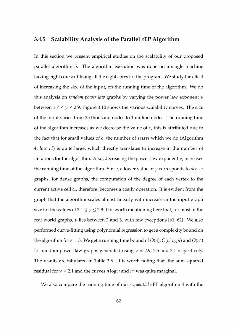
3.4.5 Scalability Analysis of the Parallel εEP Algorithm

In this section we present empirical studies on the scalability of our proposed

parallel algorithm 5. The algorithm execution was done on a single machine

having eight cores; utilizing all the eight cores for the program. We study the effect

of increasing the size of the input, on the running time of the algorithm. We do

this analysis on random power law graphs by varying the power law exponent γ

between 1.7 ≤ γ ≤ 2.9. Figure 3.10 shows the various scalability curves. The size

of the input varies from 25 thousand nodes to 1 million nodes. The running time

of the algorithm increases as we decrease the value of ε, this is attributed due to

the fact that for small values of ε, the number of splits which we do (Algorithm

4, line 11) is quite large, which directly translates to increase in the number of

iterations for the algorithm. Also, decreasing the power law exponent γ, increases

the running time of the algorithm. Since, a lower value of γ corresponds to denser

graphs, for dense graphs, the computation of the degree of each vertex to the

current active cell ca, therefore, becomes a costly operation. It is evident from the

graph that the algorithm scales almost linearly with increase in the input graph

size for the values of 2.1 ≤ γ ≤ 2.9. It is worth mentioning here that, for most of the

real-world graphs, γ lies between 2 and 3, with few exceptions [61, 62]. We also

performed curve-fitting using polynomial regression to get a complexity bound on

the algorithm for ε = 5. We get a running time bound of O(n), O(n log n) and O(n2)

for random power law graphs generated using γ = 2.9, 2.5 and 2.1 respectively.

The results are tabulated in Table 3.5. It is worth noting that, the sum squared

residual for γ = 2.1 and the curves n log n and n2 was quite marginal.

We also compare the running time of our sequential εEP algorithm 4 with the

62

epsilon = 2 epsilon = 5 epsilon = 8

Number of Nodes

Time(seconds)

Power lawexp = 1.7

exp = 2.1

exp = 2.5

exp = 2.9

ScalabilityAnalysis

1M75K50K25K1M75K50K25K1M75K50K25K

30000

60000

90000

Figure 3.10: Scalability Curve for Size of the input versus Time, for varying Power lawexponents and ε = 2, 5, 8. Higher values of power-law exponent γ signifysparse graphs, this implies, our algorithm is linearly scalable for large sparsegraphs, irrespective of the choice of ε.

γ 2.9 2.5 2.1Complexity O(n) O(n log n) O(n2)

Table 3.5: Computational Aspects of the Scalable EEP Algorithm: Curve Fitting Results,ε = 5

MapReduce based parallel algorithm 5 for sparse graphs. We perform the study

using random power-law graphs for node sizes between [5000, 75000], for the

power-law exponent γ = 2.9. The results are depicted in Figure 3.11. It is evident

from the graph that as the size of the input increases, the execution time of the

parallel algorithm decreases significantly as compared to the sequential algorithm.

For the power-law graph of 75000 nodes, we achieve a speed-up of 5X and 14X

with the parallel algorithm for ε values of 2 and 4 respectively. A smaller value of

ε in the ε-equitable partitioning algorithm translates to more number of iterations,

thereby increasing the execution time. This implies that our parallel εEP algorithm

gives us significant speed-ups over the sequential algorithm for large sparse graphs.

63

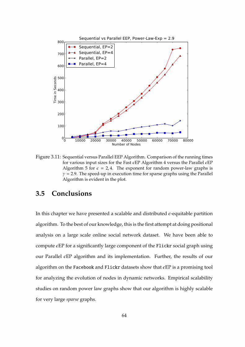
0 10000 20000 30000 40000 50000 60000 70000 80000Number of Nodes

0

100

200

300

400

500

600

700

800

Tim

e in

Sec

onds

Sequential vs Parallel EEP, Power-Law-Exp = 2.9

Sequential, EP=2Sequential, EP=4Parallel, EP=2Parallel, EP=4

Figure 3.11: Sequential versus Parallel EEP Algorithm. Comparison of the running timesfor various input sizes for the Fast εEP Algorithm 4 versus the Parallel εEPAlgorithm 5 for ε = 2, 4. The exponent for random power-law graphs isγ = 2.9. The speed-up in execution time for sparse graphs using the ParallelAlgorithm is evident in the plot.

3.5 Conclusions

In this chapter we have presented a scalable and distributed ε-equitable partition

algorithm. To the best of our knowledge, this is the first attempt at doing positional

analysis on a large scale online social network dataset. We have been able to

compute εEP for a significantly large component of the Flickr social graph using

our Parallel εEP algorithm and its implementation. Further, the results of our

algorithm on the Facebook and Flickr datasets show that εEP is a promising tool

for analyzing the evolution of nodes in dynamic networks. Empirical scalability

studies on random power law graphs show that our algorithm is highly scalable

for very large sparse graphs.

64

CHAPTER 4

Discovering Positions Performing Multiple Roles:

Multiple Epsilon Equitable Partitions

In the previous chapters we have seen that ε-equitable partitioning of a graph

corresponds to intuitive positions in networks and overcomes a lot of problems

associated with the traditional approaches of positional analysis. In this chapter

we discuss about the fact that ε-equitable partitioning of a graph is not unique

and multiple such partitions exist for a given graph. We exploit these multiple

ε-equitable partitions to analyze multiple roles and positions. We define a new

notion of equivalence based on these multiple ε-equitable partitions (MεEPs) to

perform positional analysis of social networks.

The rest of the chapter is organized as follows. In Section 4.1 we show using an

example that the εEP of a graph is not unique. Section 4.2 speaks about motivation

behind multiple role analysis in networks. We discuss the MεEPs algorithm and

its implementation in Section 4.3. In Sections 4.4 and 4.5, we define a new notion of

equivalence using the actor-actor similarity score derived from these multiple εEPs.

We present a detailed description on the evaluation methodology, ground-truth &

temporal datasets used for evaluation, and qualitative & dynamic analysis of our

proposed method in Section 4.6.

A

BD

C

I

J

GF

E

K

H

L

MNO

P

Q

R

S T

(a) Equitable Partition

A

BD

C L

MNO

P

I

J

GF

E

K

H

Q

R

S T

(b) First 1-Equitable Partition (εEP-1)

A

BD

C

I

J

GF

E

K

H

L

MNO

P

Q

R

S T

(c) Second 1-Equitable Partition (εEP-2)

Figure 4.1: (a) The TA Network under Equitable Partition is[{A},{B},{C},{D},{E-K},{L-P},{Q-T}]. (b) First 1-Equitable Partition is[{A,L-P,Q-T},{B},{C,D},{E-K}]. (c) Second 1-Equitable Partition is[{A},{B},{C,D},{E–T}]. The ε-equitable partition of a graph is not unique.

4.1 On Non-Uniqueness of ε-Equitable Partition

The evaluation of the proposed Fast εEP Algorithm 4 on the TA Network in Chapter

3, Figure: 3.2 showed that the εEP of a graph is not unique. In this section, we

work an example on the TA Network to get two different εEPs. We start with

two different cell orderings of the node degree vectors (Equation 2.6) of the input

equitable partition. Primarily, we ignore the sort by cell degrees step - line 1 of the

Algorithm 2 and shuffle the cells of the input equitable partition (EP) randomly.

The degree vectors (DVs) of the nodes of the input equitable partition, sorted by the

order their of block/cell degrees of the TA Network (Figure: 4.1a) are depicted in

Table 4.1.

Since the nodes E,F,G, ...,K all belong to the same cell of the equitable partition

of the TA Network, their DV to all the other cells of the EP are exactly the same.

Same applies to the nodes L, ...,P and Q, ...,T.

The equitable partition and the two 1-equitable partitions are shown in Figure:

4.1. For generating the first 1-equitable partition εEP-1, we start with the shuffled

cell order [{L, ...,P}, {Q, ...,T}, {A}, {C}, {B}, {D}, {E, ...,K}]. We take two consecutive

cells and try to merge them into a single cell if they are within ε = 1 of each

66

Cell Order→ 1 2 3 4 5 6 7

DV of Nodes ↓ {E,...,K} {L,...,P} {Q,...,T} {A} {D} {C} {B}−−→deg(E − K) 0 0 0 0 0 0 1−−→deg(L − P) 0 0 0 0 0 1 0−−→deg(Q − T) 0 0 0 0 1 0 0−−→deg(A) 0 0 0 0 1 1 1−−→deg(D) 0 0 4 1 0 0 0−−→deg(C) 0 5 0 1 0 0 0−−→deg(B) 7 0 0 1 0 0 0

Table 4.1: Node DVs of the TA Network’s Equitable Partition (Figure: 4.1a) in SortedOrder of their Cell Degrees

other. For further merging, this new cell becomes the current cell and is compared

with next cell for possible merger. If the merging fails, the next cell becomes the

current cell. The algorithm exits if no further merging of cells is possible. Also,

the degree vectors need to be updated whenever two cells are merged∗. The cell

merges and the corresponding DVs for εEP-1 (Figure: 4.1b) and εEP-2 (Figure:

4.1c) are depicted in Table: 4.2 and Table: 4.3 respectively. The shuffled cell order for

generating the second 1-equitable partition is [{E, ...,K}, {L, ...,P}, {Q, ...,T}, {C}, {D},

{B}, {A}]. At each step, the degree vectors of only those nodes which take part in

merging, or, are possible candidates for a merge operation are shown.

∗A detailed note on the Algorithm is given in Chapter 2, Section 2.5.3

67

DV of Equitable Partition before merge-

Cell Order→ 1 2 3 4 5 6 7

DV of Nodes ↓ {L,...,P} {Q,...,T} {A} {C} {D} {B} {E,...,K}−−→deg(L − P) 0 0 0 1 0 0 0−−→deg(Q − T) 0 0 0 0 1 0 0

DV of 1-Equitable Partition after first merge-

Cell Order→ 1 3 4 5 6 7

DV of Nodes ↓ {L,...,P,Q,...,T} {A} {C} {D} {B} {E,...,K}−−→deg(L − T) 0 0 1 1 0 0−−→deg(A) 0 0 1 1 1 0

DV of 1-Equitable Partition after second merge-

Cell Order→ 1 4 5 6 7

DV of Nodes ↓ {L,...,T,A} {C} {D} {B} {E,...,K}−−→deg(A,L − T) 0 6 5 1 0−−→deg(C) 6 0 0 0 0−−→deg(D) 5 0 0 0 0

DV of 1-Equitable Partition after third (final) merge-

Cell Order→ 1 4 6 7

DV of Nodes ↓ {L,...,T,A} {C,D} {B} {E,...,K}−−→deg(C −D) 6 0 0 0−−→deg(B) 1 0 0 7−−→deg(E − K) 0 0 1 0

Table 4.2: Epsilon equitable partition of a graph is not unique. First 1-Equitable PartitionεEP-1 is shown in Figure 4.1b. We derive this from the shuffled starting cellorder: [{L, ...,P}, {Q, ...,T}, {A}, {C}, {B}, {D}, {E, ...,K}] of the Equitable Partitiondepicted Figure 4.1a.

68

DV of Equitable Partition before merge-

Cell Order→ 1 2 3 4 5 6 7

DV of Nodes ↓ {E,...,K} {L,...,P} {Q,...,T} {C} {D} {B} {A}−−→deg(E − K) 0 0 0 0 0 1 0−−→deg(L − P) 0 0 0 1 0 0 0

DV of 1-Equitable Partition after first merge-

Cell Order→ 1 3 4 5 6 7

DV of Nodes ↓ {E,...,K,L,...,P} {Q,...,T} {C} {D} {B} {A}−−→deg(E − P) 0 0 1 0 1 0−−→deg(Q − T) 0 0 0 1 0 0

DV of 1-Equitable Partition after second merge-

Cell Order→ 1 4 5 6 7

DV of Nodes ↓ {E,...,Q,...,T} {C} {D} {B} {A}−−→deg(E − T) 0 1 1 1 0−−→deg(C) 5 0 0 0 1−−→deg(D) 4 0 0 0 1

DV of 1-Equitable Partition after third (final) merge-

Cell Order→ 1 4 6 7

DV of Nodes ↓ {E,...,T} {C,D} {B} {A}−−→deg(C −D) 9 0 0 2−−→deg(B) 7 0 0 1−−→deg(A) 0 2 1 0

Table 4.3: Epsilon equitable partition of a graph is not unique. Second 1-EquitablePartition εEP-2 is shown in Figure 4.1c. We derive this from the shuffledstarting cell order: [{E, ...,K}, {L, ...,P}, {Q, ...,T}, {C}, {D}, {B}, {A}] of the EquitablePartition depicted in Figure 4.1a.

69

4.2 Motivation

In Chapter 2 we saw that the Classical approaches to Positional Analysis, such as

Structural Equivalence, Regular equivalence, Graph Automorphisms and Equitable

Partitions, are too strict in grouping actors and often lead to trivial partitioning of

nodes in real world networks. An ε-equitable partition of the graph is a useful

relaxation to the notion of structural equivalence and often corresponds to intuitive

notions of roles and positions. All these methods assume a single role per actor,

which may not be always true in the real world. For example, a Professor can

possibly play the role of “Advisor” to students, but the role of “Colleague” to

his fellow professors. An observation we made from εEP method in the previous

section was that the initial order in which the algorithm groups actors may affect

the final position of an actor. A different starting order for the algorithm may

therefore allow us to analyze these “multiple” roles and positions in a better way.

This drives us to explore the fact that εEP of a graph is not unique and many

such partitions exist. These multiple partitions give us a better bound on grouping

actors and better insights into the “roles”. We propose a similarity score for

two actors based on their co-occurrence at a same position across multiple εEPs.

We define a new notion of equivalence using these pairwise similarity scores to

perform hierarchical clustering and identify the set of equivalent actors.

70

4.3 Algorithm for finding Multiple Epsilon Equitable

Partitions

The implementation of our algorithm is based on the modification of Kate’s [1]

Algorithm 2 to find an εEP of a graph. The algorithm to find the multiple

ε-equitable partitions of a graph is presented in Algorithm box 6. Input to our

algorithm is (i) the graph, (ii) the coarsest equitable partition of graph, (iii) a value of

ε and (iv) r - the number of εEPs required.

The algorithm performs a common pre-processing step (Algorithm 6, lines 1−10)

for all the r MεEPs it returns. Pre-processing involves merging all the cells of the EP

which have cell degrees between [0, ε/2]. We derive this heuristic by combining

the two observations† made by the author in [1]. The two observations are as

follows:

• Observation 1: Merging the cells of an equitable partition having same

degree such that it is less than ε does not violate the ε condition of an

ε-equitable partition.

• Observation 2: Merging cells according to the criterion with ε = ε/2 does

not violate the ε condition for other cells.

The pre-processing step of our Algorithm 6 differs from the pre-processing step

(lines 2− 5) of Kate’s Algorithm 2. In Algorithm 2, for each degree i ∈ 0→ ε, a new

cell corresponding to the degree i merges all the cells from EP having a cell degree

= i. Further, these (ε+1) new cells are excluded for subsequent merge operations of

†For details and proofs, interested readers may please refer Chapter 4, Section 4.3.4 of [1].

71

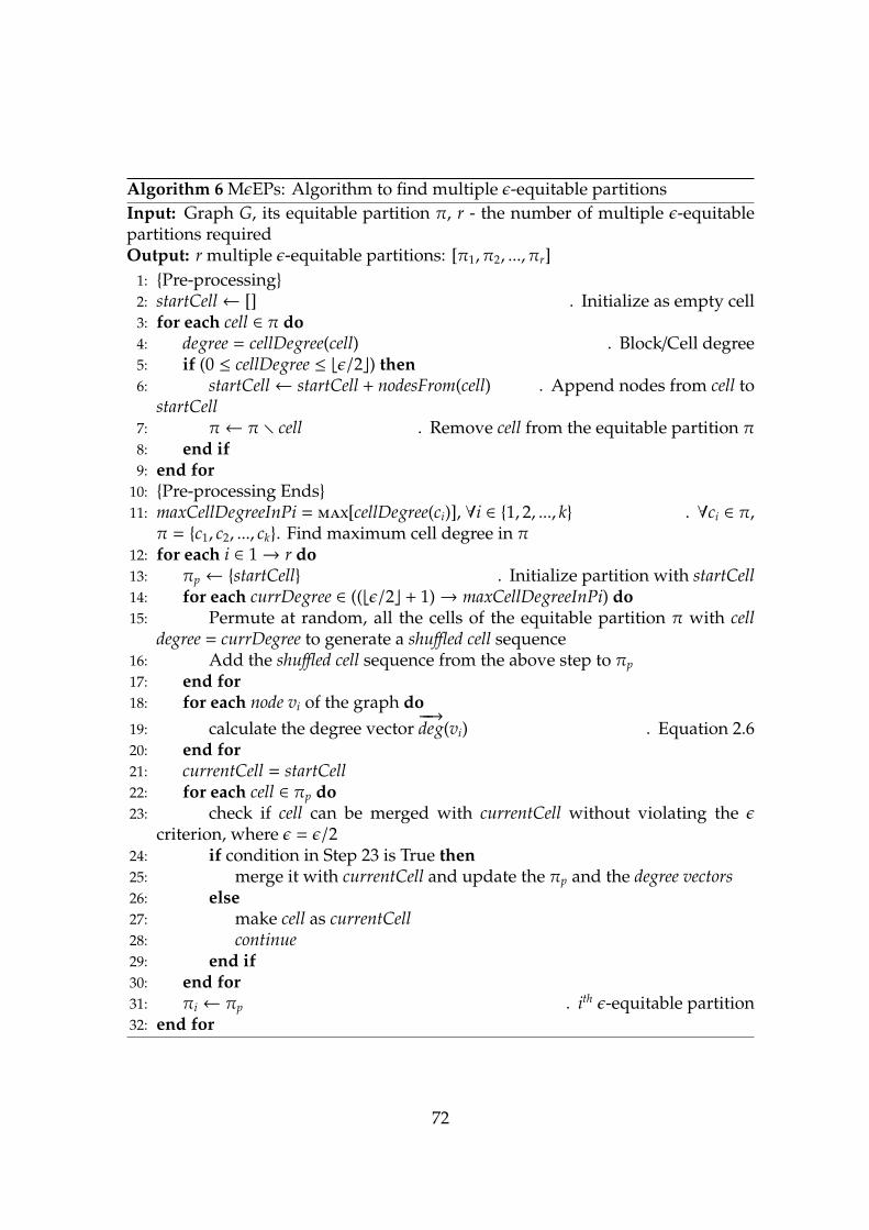
Algorithm 6 MεEPs: Algorithm to find multiple ε-equitable partitionsInput: Graph G, its equitable partition π, r - the number of multiple ε-equitablepartitions requiredOutput: r multiple ε-equitable partitions: [π1, π2, ..., πr]

1: {Pre-processing}2: startCell← [] . Initialize as empty cell3: for each cell ∈ π do4: degree = cellDegree(cell) . Block/Cell degree5: if (0 ≤ cellDegree ≤ bε/2c) then6: startCell← startCell + nodesFrom(cell) . Append nodes from cell to

startCell7: π← π r cell . Remove cell from the equitable partition π8: end if9: end for

10: {Pre-processing Ends}11: maxCellDegreeInPi = max[cellDegree(ci)], ∀i ∈ {1, 2, ..., k} . ∀ci ∈ π,

π = {c1, c2, ..., ck}. Find maximum cell degree in π12: for each i ∈ 1→ r do13: πp ← {startCell} . Initialize partition with startCell14: for each currDegree ∈ ((bε/2c + 1)→ maxCellDegreeInPi) do15: Permute at random, all the cells of the equitable partition π with cell

degree = currDegree to generate a shuffled cell sequence16: Add the shuffled cell sequence from the above step to πp

17: end for18: for each node vi of the graph do19: calculate the degree vector

−−→deg(vi) . Equation 2.6

20: end for21: currentCell = startCell22: for each cell ∈ πp do23: check if cell can be merged with currentCell without violating the ε

criterion, where ε = ε/224: if condition in Step 23 is True then25: merge it with currentCell and update the πp and the degree vectors26: else27: make cell as currentCell28: continue29: end if30: end for31: πi ← πp . ith ε-equitable partition32: end for

72

the algorithm. In our Algorithm 6, we combine the above two observations. First,

we create a single new startCell having the nodes from all the cells whose cell degree

i ∈ 0 → ε/2. Second, we allow this cell to be a valid starting cell for subsequent

merge comparisons. Since the cell degree of startCell is at most ε/2, it follows from

Observation 2 that the startCell does not violate the ε condition for other cells in the

subsequent merges. The cells which are added to the startCell are removed from

the input EP (line 7, Algorithm 6). The algorithm then generates r random cell order

permutations within cell degrees for all the remaining cells of the input EP (lines

12−17, Algorithm 6). This corresponds to generating r different starting shuffled cell

order sequences for finding multiple εEPs. We restrict the shuffling of the cells within

each cell degree of the input EP π. We adopt this heuristic to maximize the chances

of possible cell merges according to the ε criterion, since the likelihood of merging

two cells with an equal cell degree is more than the cells with differing cell degrees.

The algorithm then computes the DVs of all the nodes (lines 18− 20, Algorithm 6).

The algorithm then tries to merge these cells by taking two consecutive cells at a

time. If the degree vectors of the member nodes from these two cells are within ε/2

distance of each other, they are merged into a single new cell. For further merging,

this new cell becomes the current cell, which is then compared with the next cell

for a possible merger. If the merging fails, the next cell becomes the current cell

(lines 21− 30, Algorithm 6). Also, the degree vectors need to be updated whenever

two cells are merged. If no further merging of cells is possible, the partition is

returned as the ith ε-equitable partition πi (line 31, Algorithm 6). A loose bound on

the running time complexity of Algorithm 6 is O(r.n3), where r is the number of

ε-equitable partitions and n being the size of the vertex set V ∈ G. We present an

efficient parallel implementation of the algorithm in the following subsection.

73

4.3.1 Implementation of the MεEPs Algorithm

In the previous section we discussed that generating multiple εEPs is computationally

expensive. The Multiple εEPs algorithm generates the permutations of the initial

cells given by the equitable partition algorithm, and then computes an εEP for

each one of these permuted cell orderings. The initial computation of degree

vectors (Equation 2.6) of all the vertices of the input social graph is computationally

intensive (line 18 − 19, Algorithm 6). These degree vectors are also large in size.

We address the problem as follows: Given, the cell ordering {c1, c2, ...cK} of

the initial equitable partition πinit of a graph G, we compute the degree vectors

of the vertex-set V ∈ G corresponding to this cell order. We persist these DVs

on a hierarchical data format (HDF) file [63, 64]. HDF files are used to store and

organize large amounts of numerical data, while providing efficient access, storage

and platform independence capabilities. In the implementation of the Multiple

εEPs algorithm, for each permuted cell of πinit (lines 14 − 17, Algorithm 6), we

maintain and persist a mapping corresponding to its original cell number in πinit.

In other words, for each permuted cell of the current εEP iteration, we also maintain

a mapping of its cell index in the saved HDF file. Now given, (i) the permuted

cell ordering and (ii) its mapping to the initial cells of the equitable partition, each

MεEPs algorithm iteration can execute independently in parallel. With this, we

are also able to run this in a distributed setting by simply copying the HDF file

to each computing node and triggering the MεEPs algorithm using GNU Parallel

[54]. The following example depicts the working of shared degree vectors and a

mapping of permuted cells.

74

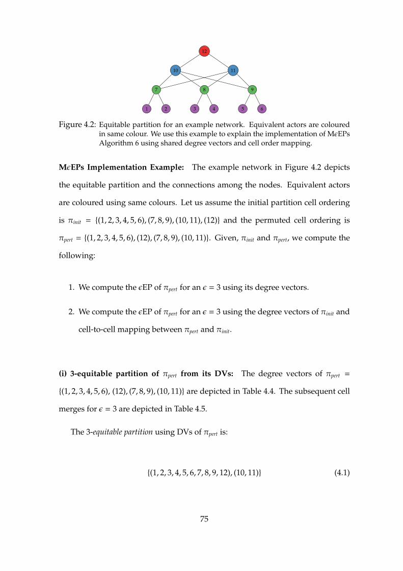
12

10 11

7 8 9

1 2 3 4 5 6

Figure 4.2: Equitable partition for an example network. Equivalent actors are colouredin same colour. We use this example to explain the implementation of MεEPsAlgorithm 6 using shared degree vectors and cell order mapping.

MεEPs Implementation Example: The example network in Figure 4.2 depicts

the equitable partition and the connections among the nodes. Equivalent actors

are coloured using same colours. Let us assume the initial partition cell ordering

is πinit = {(1, 2, 3, 4, 5, 6), (7, 8, 9), (10, 11), (12)} and the permuted cell ordering is

πpert = {(1, 2, 3, 4, 5, 6), (12), (7, 8, 9), (10, 11)}. Given, πinit and πpert, we compute the

following:

1. We compute the εEP of πpert for an ε = 3 using its degree vectors.

2. We compute the εEP of πpert for an ε = 3 using the degree vectors of πinit and

cell-to-cell mapping between πpert and πinit.

(i) 3-equitable partition of πpert from its DVs: The degree vectors of πpert =

{(1, 2, 3, 4, 5, 6), (12), (7, 8, 9), (10, 11)} are depicted in Table 4.4. The subsequent cell

merges for ε = 3 are depicted in Table 4.5.

The 3-equitable partition using DVs of πpert is:

{(1, 2, 3, 4, 5, 6, 7, 8, 9, 12), (10, 11)} (4.1)

75

Cell Order→ Cell1 Cell2 Cell3 Cell4

DV of Nodes ↓ {1, 2, ..., 6} {12} {7, 8, 9} {10, 11}−−→deg(1) 0 0 1 0−−→deg(12) 0 0 0 2−−→deg(7) 2 0 0 2−−→deg(10) 0 1 3 0

Table 4.4: The cell DVs of the example network of Figure 4.2, corresponding to the cellorder of πpert.

(ii) 3-equitable partition of πpert from DVs of πinit and cell mapping: The degree

vectors of πinit = {(1, 2, 3, 4, 5, 6), (7, 8, 9), (10, 11), (12)} are depicted in Table 4.6. The

cell-to-cell mapping between the cells of πinit and πpert is shown in Table 4.7. The

subsequent cell merges for ε = 3 are depicted in Table 4.8.

The 3-equitable partition using DVs of πinit and cell-to-cell mapping between πinit

and πpert is:

{(1, 2, 3, 4, 5, 6, 7, 8, 9, 12), (10, 11)} (4.2)

The example shows that the εEP computed using the node DVs of the initial

equitable partition cell ordering and a cell-to-cell mapping (Eq. 4.2), is exactly

same, as the εEP computed using the node DVs of the permuted cell ordering (Eq.

4.1) of the input graph’s equitable partition.

This implementation helped us achieve parallelism and a significant reduction

in the memory footprint. Since, for generating n multiple εEPs, we only save n

mapping files and a single instance of the node degree vectors HDF file on disk.

Thus, we avoid recomputation and storage of n times the size of degree vectors of

the vertex-set V.

76

DV after 1st Merge: Cell1 ← Cell1 + Cell2

Cell Order→ Cell1 Cell3 Cell4

DV of Nodes ↓ {1, 2, ..., 6} {7, 8, 9} {10, 11}−−→deg(1) 0 1 0−−→deg(12) 0 0 2−−→deg(7) 2 0 2−−→deg(10) 1 3 0

DV after 2nd Merge: Cell1 ← Cell1 + Cell3

Cell Order→ Cell1 Cell4

DV of Nodes ↓ {1, 2, ..., 6} {10, 11}−−→deg(1) 1 0−−→deg(12) 0 2−−→deg(7) 2 2−−→deg(10) 4 0

Table 4.5: Cell merge sequence of the example network of Figure 4.2 for ε = 3. The cellorder corresponds to that of the partition πpert (Table 4.4).

Cell Order→ Cell1 Cell2 Cell3 Cell4

DV of Nodes ↓ {1, 2, ..., 6} {7, 8, 9} {10, 11} {12}−−→deg(1) 0 1 0 0−−→deg(7) 2 0 2 0−−→deg(10) 0 3 0 1−−→deg(12) 0 0 2 0

Table 4.6: The cell DVs of the example network of Figure 4.2, corresponding to the cellorder of πinit.

77

πinit Cell1 Cell2 Cell3 Cell4

πpert Cell1 Cell4 Cell2 Cell3

Table 4.7: Cell-to-cell mapping between πinit and πpert for the cell orderings of ExampleNetwork of Figure 4.2.

DV after 1st Merge: Cell1 ← Cell1 + Cell4

Cell Order→ Cell1 Cell2 Cell3

DV of Nodes ↓ {1, 2, ..., 6} {7, 8, 9} {10, 11}−−→deg(1) 0 1 0−−→deg(7) 2 0 2−−→deg(10) 1 3 0−−→deg(12) 0 0 2

DV after 2nd Merge: Cell1 ← Cell1 + Cell2

Cell Order→ Cell1 Cell3

DV of Nodes ↓ {1, 2, ..., 6} {10, 11}−−→deg(1) 1 0−−→deg(7) 2 2−−→deg(10) 4 0−−→deg(12) 0 2

Table 4.8: Cell merge sequence of the example network of Figure 4.2 for ε = 3. Thecell order corresponds to that of the partition πinit (Table 4.6) and each mergesequence is mapped to πpert using the cell-to-cell mapping from the Table 4.7.

78

4.4 Actor-Actor Similarity Score

In this section we define the notion of actor-actor similarity score, which forms the

basis for the definition of a “Position in MεEPs”. Given, nodes vi, v j ∈ G and

n multiple ε-equitable partitions {π1, π2, ..., πn} of G. We introduce the following

definitions:

Definition 4.1. (Common Cell Members) Given, nodes vi, v j and partition π =

{c1, c2, ..., ck}. We define a boolean function cellMembersπ(vi, v j) on the partition π as

follows:

cellMembersπ(vi, v j) =

1, if (vi ∈ cr and v j ∈ cr), for some cr ∈ π.

0, otherwise.

(4.3)

The function cellMembersπ returns a value of 1 (true), if the nodes vi and v j both

belong to the same cell or block of the partition π.

Definition 4.2. (Actor-Actor Co-occurrence) Given, two nodes vi, v j and the partitions

{π1, π2, ..., πn}. We define the co-occurrence function cooc(vi, v j) as follows:

cooc(vi, v j) =

n∑k=1

cellMembersπk(vi, v j) (4.4)

This function essentially returns the count of the number of partitions in which the

node-pair vi, v j occupies a same position in the partition.

79

EEP1

EEP2

EEP3

a,b

EEP1

EEP2

EEP3a,c

EEP1

EEP2

EEP3

d,e

Figure 4.3: Example of Actor-Actor Similarity for three ε-equitable partitions usingEquation 4.5. (a) sim(a, b) = 1. (b) sim(a, c) = 1/3. (c) sim(d, e) = 2/3.

Definition 4.3. (Actor-Actor Similarity and Distance) Given, a nodes vi, v j ∈ G and

the partitions {π1, π2, ..., πn}. The similarity and distance between two nodes vi and

v j is defined as:

sim(vi, v j) =cooc(vi, v j)

n(4.5)

dist(vi, v j) = 1 − sim(vi, v j) (4.6)

Thus, the similarity score of two actors vi and vi is defined as the number of

εEPs in which both vi and v j occupy a same position, divided by the total number

of multiple ε-equitable partitions generated for the graph G.

Following example illustrates the actor-actor similarity for three ε−equitable

partitions. The example is also depicted in the Figure 4.3.

• EEP1: {(a,b,c),(d,e),(f)}

• EEP2: {(a,b),(d,e),(c,f)}

• EEP3: {(a,b),(c,d),(e,f)}

• sim(a, b) = 1, sim(a, c) = 1/3, sim(a, d) = 0

• dist(a, b) = 0, dist(a, c) = 2/3, dist(a, d) = 1

80

4.5 Definition of a “Position” in Multiple ε-Equitable

Partitions

In this section, we define the notion of a “Position” in MεEPs. Before that, we define

some preliminaries in the coming subsections.

4.5.1 Hierarchical Clustering

Hierarchical Clustering (HC) [65] builds a hierarchy of clusters which are used to

perform cluster analysis. The strategies to perform HC fall under two categories:

1. Hierarchical Agglomerative Clustering: This is a bottom-up approach at

creating cluster hierarchies. Hierarchical Agglomerative Clustering (HAC)

starts with each node as a singleton cluster at the outset and then successively

merge/agglomerate pairs of clusters using a linkage criterion based on the node

similarity/distance scores. The merge terminates when all clusters have been

merged into a single cluster that contains all the nodes.

2. Hierarchical Divisive Clustering: This is a top-down approach to create

cluster hierarchies. Divisive clustering starts with a single cluster containing

all the nodes at the outset. It proceeds by splitting clusters recursively at each

step until individual nodes are reached.

Linkage Criteria for HAC: The HAC algorithm depends on a linkage criterion to

agglomerate a pair of clusters at each level of hierarchy. Given, the n × n distance

matrix dist which contains the pairwise distance between each of the n node-pairs

81

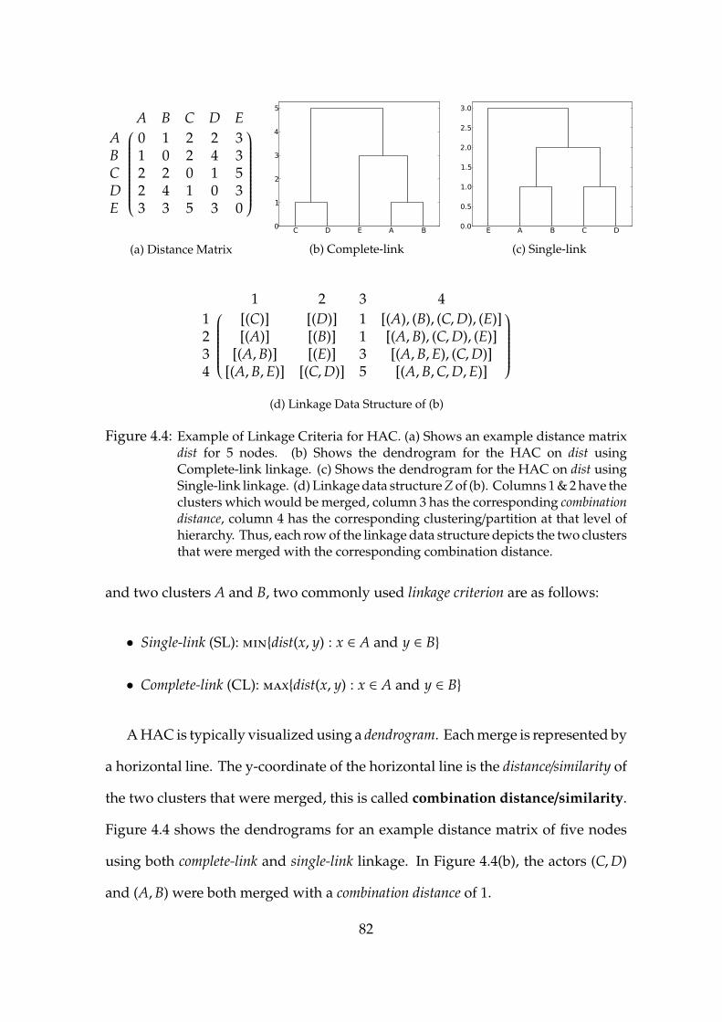
A B C D EA 0 1 2 2 3B 1 0 2 4 3C 2 2 0 1 5D 2 4 1 0 3E 3 3 5 3 0

(a) Distance Matrix

C D E A B0

1

2

3

4

5

(b) Complete-link

E A B C D0.0

0.5

1.0

1.5

2.0

2.5

3.0

(c) Single-link

1 2 3 4

1 [(C)] [(D)] 1 [(A), (B), (C,D), (E)]2 [(A)] [(B)] 1 [(A,B), (C,D), (E)]3 [(A,B)] [(E)] 3 [(A,B,E), (C,D)]4 [(A,B,E)] [(C,D)] 5 [(A,B,C,D,E)]

(d) Linkage Data Structure of (b)

Figure 4.4: Example of Linkage Criteria for HAC. (a) Shows an example distance matrixdist for 5 nodes. (b) Shows the dendrogram for the HAC on dist usingComplete-link linkage. (c) Shows the dendrogram for the HAC on dist usingSingle-link linkage. (d) Linkage data structure Z of (b). Columns 1 & 2 have theclusters which would be merged, column 3 has the corresponding combinationdistance, column 4 has the corresponding clustering/partition at that level ofhierarchy. Thus, each row of the linkage data structure depicts the two clustersthat were merged with the corresponding combination distance.

and two clusters A and B, two commonly used linkage criterion are as follows:

• Single-link (SL): min{dist(x, y) : x ∈ A and y ∈ B}

• Complete-link (CL): max{dist(x, y) : x ∈ A and y ∈ B}

A HAC is typically visualized using a dendrogram. Each merge is represented by

a horizontal line. The y-coordinate of the horizontal line is the distance/similarity of

the two clusters that were merged, this is called combination distance/similarity.

Figure 4.4 shows the dendrograms for an example distance matrix of five nodes

using both complete-link and single-link linkage. In Figure 4.4(b), the actors (C,D)

and (A,B) were both merged with a combination distance of 1.

82

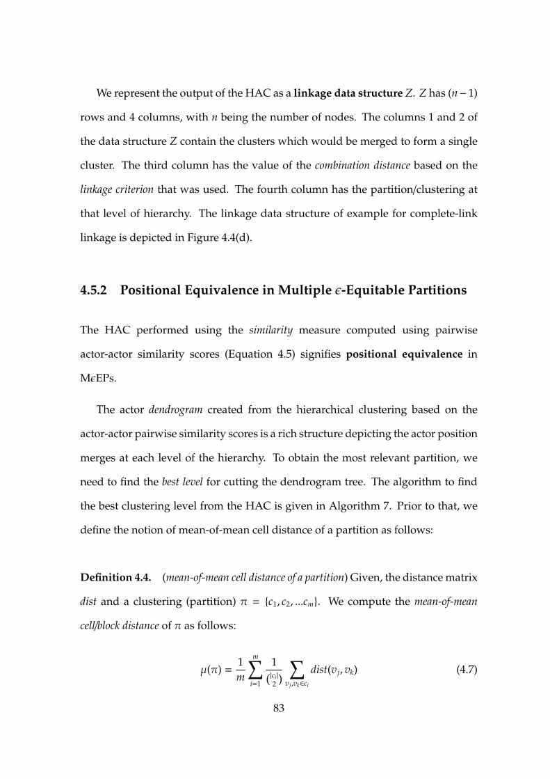
We represent the output of the HAC as a linkage data structure Z. Z has (n−1)

rows and 4 columns, with n being the number of nodes. The columns 1 and 2 of

the data structure Z contain the clusters which would be merged to form a single

cluster. The third column has the value of the combination distance based on the

linkage criterion that was used. The fourth column has the partition/clustering at

that level of hierarchy. The linkage data structure of example for complete-link

linkage is depicted in Figure 4.4(d).

4.5.2 Positional Equivalence in Multiple ε-Equitable Partitions

The HAC performed using the similarity measure computed using pairwise

actor-actor similarity scores (Equation 4.5) signifies positional equivalence in

MεEPs.

The actor dendrogram created from the hierarchical clustering based on the

actor-actor pairwise similarity scores is a rich structure depicting the actor position

merges at each level of the hierarchy. To obtain the most relevant partition, we

need to find the best level for cutting the dendrogram tree. The algorithm to find

the best clustering level from the HAC is given in Algorithm 7. Prior to that, we

define the notion of mean-of-mean cell distance of a partition as follows:

Definition 4.4. (mean-of-mean cell distance of a partition) Given, the distance matrix

dist and a clustering (partition) π = {c1, c2, ...cm}. We compute the mean-of-mean

cell/block distance of π as follows:

µ(π) =1m

m∑i=1

1(|ci|

2

) ∑v j,vk∈ci

dist(v j, vk) (4.7)

83

For each unique pair of vertices in a cell, we compute the mean of distances

between these pairs and then we compute the mean of these means.

Algorithm 7 Best Level to Cut the Dendrogram TreeInput: (i) HAC linkage data structure Z and (ii) threshold range [τ1, τ2]Output: Clustering π of G

1: d1 = 0.0 . Initialize previous combination distance2: µ1 = 0.0 . Initialize previous mean-of-mean cell distance of π3: max slope = 0.0 . Initialize maximize slope4: best level = 0 . Initialize best clustering level5: for each level in Z do . Iterate over each row in the HAC linkage matrix Z6: π = clusteringAt(level) = Z[level][4] . π is the clustering/partition at the

level: level in Z7: µ2 = µ(π) . mean-of-mean cell distance of π, Equation 4.78: d2 = Z[level][3] . the combination distance at level: level of HAC9: slope =

µ2−µ1

d2−d1. rate-of-change of mean-of-mean cell distance w.r.t

combination distance10: if (τ1 ≤ µ2 ≤ τ2) and (slope > max slope) then11: max slope = slope . Update max slope12: best level = (level − 1) . best level is previous level, since there was a

change of slope between the current level and previous level13: end if14: µ1 = µ2 . Update µ1 and d1 for next iteration15: d1 = d2

16: end for17: π = clusteringAt(best level) = Z[best level][4]18: return π . Return the best clustering from HAC

Algorithm 7: Best Level to Cut the Dendrogram Tree The algorithm to find the

best clustering from the dendrogram tree is given in Algorithm 7. The input to the

algorithm is (i) HAC linkage data structure and (ii) threshold range [τ1, τ2]. The

algorithm iterates over each level of the HAC linkage structure Z and evaluates

the following. At each level of the hierarchy, algorithm takes the partition π

corresponding to the clustering at that level of HAC. It computes the mean-of-mean

84

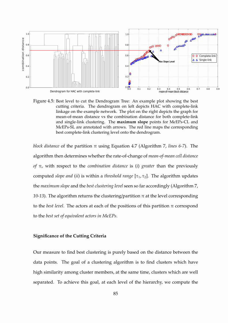
0.0

0.2

0.4

0.6

0.8

1.0

0.0 0.1 0.2 0.3 0.4 0.5 0.6 0.7 0.8 0.9mean-of-meanblockdistanceDendrogram for HAC with complete-link

0.0

0.2

0.4

0.6

0.8

1.0

com

bin

ati

on

dis

tance

Max Slope LevelMax Slope Level

Complete-link

Single-link

Figure 4.5: Best level to cut the Dendrogram Tree: An example plot showing the bestcutting criteria. The dendrogram on left depicts HAC with complete-linklinkage on the example network. The plot on the right depicts the graph formean-of-mean distance vs the combination distance for both complete-linkand single-link clustering. The maximum slope points for MεEPs-CL andMεEPs-SL are annotated with arrows. The red line maps the correspondingbest complete-link clustering level onto the dendrogram.

block distance of the partition π using Equation 4.7 (Algorithm 7, lines 6-7). The

algorithm then determines whether the rate-of-change of mean-of-mean cell distance

of π, with respect to the combination distance is (i) greater than the previously

computed slope and (ii) is within a threshold range [τ1, τ2]. The algorithm updates

the maximum slope and the best clustering level seen so far accordingly (Algorithm 7,

10-13). The algorithm returns the clustering/partition π at the level corresponding

to the best level. The actors at each of the positions of this partition π correspond

to the best set of equivalent actors in MεEPs.

Significance of the Cutting Criteria

Our measure to find best clustering is purely based on the distance between the

data points. The goal of a clustering algorithm is to find clusters which have

high similarity among cluster members, at the same time, clusters which are well

separated. To achieve this goal, at each level of the hierarchy, we compute the

85

mean-of-mean block distance of the partition using Equation 4.7. We compute the

rate-of-change of mean-of-mean block distance, with respect to the change in cluster

combination distance (Section 4.5.1). The comparison of the current slope, with the

slope computed for the previous level of clustering hierarchy iteratively capture

the drastic changes in the slope as maximum slope. The updates to maximum slope

also update the best level in the dendrogram tree seen so far. We also restrict the

threshold range for the mean-of-mean cell distance of partition as [τ1 = 0.15, τ2 = 0.35].

The mean-of-mean block distance value of τ1 = 0.15 is fixed based on empirical

studies. We didn’t get any meaningful roles for smaller distance values of τ1 (i.e.,

for τ1 < 0.15). This is due to the fact that there wasn’t any level in the dendrogram

tree which corresponds to a mean-of-mean block distance< 0.15. The upper bound

of τ2 = 0.35 ensured that the intra position actor-actor similarity for all positions in

the partition is at least 65%. Note that, from Equation 4.5 and 4.6, these thresholds

correspond to a bound on mean-of-mean cell similarity of a partition in the range

[0.65, 0.85]. Therefore, the slope and threshold range correspond to an objective

function which finds a level in the tree having the following significance:

• The mean of “the intra-position actor-actor similarity mean” for the all the

positions in the partition is at least 65%.

• Cut the dendrogram tree at a level prior to the level which has the maximum

slope. This level corresponds to a level after which there was a drastic change

in the slope. Hence this implies that, the merge between two clusters at this

level according to the combination similarity has resulted in a drastic change

in the intra-position similarities.

86

The manuscripts [66, 67] discuss various measures for cluster quality analysis.

Evaluation of MεEPs on multi-role ground-truth networks shows that our method

correctly discovers positions performing multiple roles.

4.6 Experimental Evaluation

The datasets used for evaluation are described in Section 4.6.1, followed by the

evaluation methodology in Section 4.6.2. Finally, we present the results in Section

4.6.3.

4.6.1 Datasets used for Evaluation

Multi-Role Ground-truth Datasets:

1. Internet Movie Database Co-Cast Network The Internet Movie Database

(IMDb) [68] is an online database of movies, television shows and video games.

The database has the information related to the actors, production crew, release

date, trivia, genre, plots etc. to name a few. We create a movie Co-Cast network

as follows: The cast members are from English movies of “Action” genre between

the year 2003 to 2013. They form the nodes of the Co-Cast network. Using the

complete IMDb database, two nodes i and j are linked with a weight wi j, if they

have cast together in wi j movies. We discard links whose weight is less than 10,

corresponding isolate nodes are also discarded. We assign a role label vector for

each node in the Co-Cast network based on the role(s) they have performed while

casting in movies. For example, if we have three roles: actor, director and writer; a

node i has worked in 5 movies as an actor, 6 movies as a director and 2 movies as

87

a writer. Therefore, the role label vector for a node i will be ~ri = {5, 6, 2}. Further,

the components in the role label vector of a node having values less than 5 are

considered 0. In our example, the final role label vector for node i is ~ri = {5, 6, 0},

this essentially means that we would only consider node i in roles of actor and

director. The role label vector corresponds to the ground-truth roles. Our IMDb

dataset has 10 defined roles. The IMDb Co-Cast network consists of 7874 vertices

and 11393 edges. The degree distribution plot of the IMDb Co-Cast Network is

shown in Figure 4.6. The role distributions are given in Table 4.9.

Role Vertices PercentageActor 2498 31.72Actress 739 9.39Cinematographer 350 4.45Composer 163 2.07Costume Designer 40 0.51Director 694 8.81Editor 440 5.59Miscellaneous Crew 1723 21.88Producer 1744 22.15Writer 810 10.29

Table 4.9: IMDb Dataset Role Distributions

2. Summer School Network This is a network derived from a survey taken at

a doctoral summer school [69]. The Summer School Network (SSN) is a network

of attendees based on a survey questionnaire, which primarily asked them about

the people they knew before and after the summer school. We use the combined

network, which takes the union of links of people who knew each other (i) before

the summer school and (ii) after the summer school. The network has a link from

vertex A to vertex B, if person A responded to know person B. For our evaluation,

we assume the links to be symmetric and hence we convert the network to an

88

100 101 102 103

node degree (d)

100

101

102

103

104#

nod

es w

ith d

egre

e ≥

dDegree Distribution of IMDB Co-Cast Network

Figure 4.6: Degree distribution plot of the IMDb Co-Cast Network for English Actionmovies, between year 2003 to 2013.

undirected graph. This graph has 73 vertices and 1138 edges. Further, for each

vertex v in the network, the dataset has corresponding “roles” performed by the

person. Few roles defined for a person are: Senior Organizer, Local Organizer, Visitor,

Speaker etc., these correspond to the ground-truth roles. The role distribution is

reported in Table 4.10.

Role Vertices PercentageAttendee 54 73.97Local Organizer 18 24.66Senior Organizer 10 13.70Speaker 16 21.92Visitor 45 61.64

Table 4.10: Summer School Dataset Role Distributions

89

Datasets used for Dynamic Analysis

1. JMLR Dataset We extracted the Co-Authorship and Co-Citation networks for

the Journal of Machine Learning Research (JMLR) for the years spanning from

2001 to 2011. The dataset was extracted from Thomson Reuters Web of Science

Portal [70] and processed using the Science of Science (Sci2) toolbox [71].

We create 6 time evolving snapshots for the Co-Citation network from year 2006

to year 2011, such that, the snapshot for year 2006 network has paper co-citation

data from year 2001 to year 2006. The snapshot for year 2007 network includes

the data from year 2001 to year 2007 and so on for years up to 2011. Similarly, we

generate 2 time evolving snapshots for the Co-Authorship network for years 2010

and 2011. Further, edges with number of co-authored or co-cited papers together

with edge-weights less than 4 were pruned in the study. The dataset properties of

the final network have been tabulated in Table 4.11.

Dataset Vertices EdgesCo-Authorship 1356 2363Co-Citation 541 5672

Table 4.11: JMLR Dataset Properties

2. DBLP Co-Authorship Network We parsed the DBLP bibliographic database

[72] to extract the author details from the conference proceedings of KDD, VLDB

and ICML between year 1999 to year 2013. We generate 2 time evolving snapshots

of the co-authorship network, using the same methodology as described for the

JMLR dataset. The first network has all the co-authorship links between the years

1999 to 2008, the evolved network consists of all the links between year 1999 to

year 2013. The dataset details are tabulated in Table 4.12. The degree distribution

90

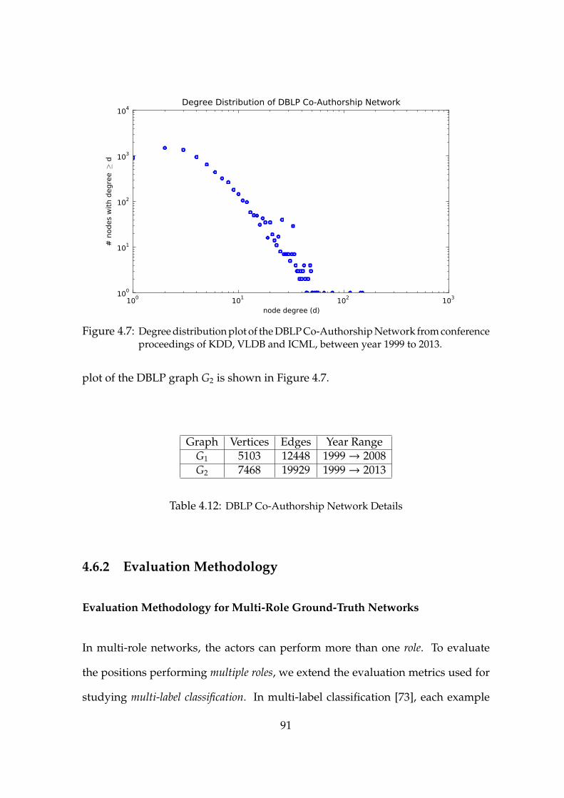
100 101 102 103

node degree (d)

100

101

102

103

104#

nod

es w

ith d

egre

e ≥

dDegree Distribution of DBLP Co-Authorship Network

Figure 4.7: Degree distribution plot of the DBLP Co-Authorship Network from conferenceproceedings of KDD, VLDB and ICML, between year 1999 to 2013.

plot of the DBLP graph G2 is shown in Figure 4.7.

Graph Vertices Edges Year RangeG1 5103 12448 1999→ 2008G2 7468 19929 1999→ 2013

Table 4.12: DBLP Co-Authorship Network Details

4.6.2 Evaluation Methodology

Evaluation Methodology for Multi-Role Ground-Truth Networks

In multi-role networks, the actors can perform more than one role. To evaluate

the positions performing multiple roles, we extend the evaluation metrics used for

studying multi-label classification. In multi-label classification [73], each example

91

xi ∈ X is associated with a set of ground-truth labels Y ⊆ L, with |L| > 2. The

multi-label classifier H predicts a set of labels Zi = H(xi), for each of the examples

xi ∈ X. The evaluation metrics that we use are as follows:

1. Hamming Loss: This was used by the authors in [74], it is defined as follows.

HammingLoss(H,D) =1|D|

|D|∑i=1

|Yi 4 Zi|

|L|(4.8)

where, |D| is the number of examples, |L| is the number of labels, Yi is the

ground-truth label set of example xi and Zi is the predicted label set of xi.

4 is the symmetric difference of two sets. Hamming loss evaluates how many

times an example and its label pair are misclassified. Smaller the value of

hamming loss, better is the performance.

2. Precision: This along with recall and accuracy were used by authors in [75].

Precision(H,D) =1|D|

|D|∑i=1

|Yi ∩ Zi|

|Zi|(4.9)

Precision is the fraction of the labeled examples which are correctly labeled.

Bigger the value of precision, better is the performance.

3. Recall: Is defined as follows.

Recall(H,D) =1|D|

|D|∑i=1

|Yi ∩ Zi|

|Yi|(4.10)

Recall is the fraction of the labeled examples which are relevant. Bigger value

of recall is better. But getting a recall value of 1 in Equation 4.10 is trivial by

labeling the predicted label set Zi of xi with the entire label set L. Hence recall

92

alone is not a good measure.

4. Accuracy: Is defined as follows.

Accuracy(H,D) =1|D|

|D|∑i=1

|Yi ∩ Zi|

|Yi ∪ Zi|(4.11)

Accuracy symmetrically measures how close the actual labels are to the

predicted labels. Bigger the value of accuracy, better it is.

5. F1 Score: Is defined as follows.

F1 =2 × precision × recall

precision + recall(4.12)

F1 score weights recall and precision equally. A good algorithm will maximize

both precision and recall.

Notion of Predicted Labels for Evaluating MεEPs Since multi-label classification

is a supervised learning approach and MεEPs is an unsupervised approach, we

extend the evaluation metrics as follows. The predicted label set Z of a vertex u,

corresponds to the union of all the ground-truth labels of the vertices which belong

to the position occupied by u, including the labels of u. This can be mathematically

defined as follows. Given, a vertex u ∈ c j, where c j is the cell of the partition π

given by our method. The predicted label Z is defined as:

Z =⋃v∈c j

{r|r ∈ ~rv and r , 0} (4.13)

where, ~rv is the role vector of vertex v.

93

Please note that, we discard the singletons from the study while computing

each of these evaluation metrics and for the evaluation metrics discussed in the

subsequent sections. All the results reported in this thesis exclude singletons. We

do this to avoid an evaluation bias. For example, in the context of ground-truth

metrics since the predicted label and the actual label for singletons would always

be the same, singletons would create an evaluation bias.

Additional Measures to Evaluate Multi-Role Networks In addition to the evaluation

measures discussed above, we also use the following two measures:

1. Np - the number of positions correctly identified performing multiple roles.

Given, a position ci and the actors a j ∈ ci, where j ∈ 1 → |ci|, i ∈ 1 → K and

the partition π = {c1, c2, ..., cK} (K is the number of positions in π). Then,

Np = sizeo f { ci | ∀a j, ak ∈ ci =⇒ ~ra j = ~rak} (4.14)

where, ~rv is the role label vector of vertex v.

2. Na - the number of actors correctly identified performing multiple roles.

Given, a position ci and the actors a j ∈ ci, where j ∈ 1 → |ci|, i ∈ 1 → K and

the partition π = {c1, c2, ..., cK} (K is the number of positions in π). Then,

Na =

K∑i=1

{sizeo f (ci) | ∀a j, ak ∈ ci =⇒ ~ra j = ~rak} (4.15)

94

Evaluation Methodology for Dynamic Analysis

Since we are primarily interested in studying the effect of PA on dynamic social

networks and to characterize what role PA plays in the co-evolution of nodes

in the networks. We follow the same evaluation strategies as discussed in the

previous Chapter 3, Section 3.4.3. In addition to the evaluation measures discussed

previously, we also study the evolution of ties of actor-pairs. We discuss this in the

following subsection.

Evolution of Ties/Links of Actor-Pairs We are primarily interested in finding out

how the ties of actor pairs, which have common membership to a position in the

network at time t, evolve over time with respect to their ties to other positions. For

each pair of nodes that share a position in the time t network, we create a difference

degree vector of their number of connections to all the other positions. For example,

if node a has two connections to position p1 and three connections to position p2,

and node b has one connection to position p1 and four connections to position p2,

their difference degree vector ~a − ~b would be [1,−1]. For same pair of actors, we

compute their difference degree vector for the time t + δt network. A natural way to

compare the degree vectors of the t and t + δt networks is using cosine similarity.

We pad the smaller of the two vectors with zeros to make its dimension equal to

the other one. Cosine similarity is the normalized dot product of two vectors and

is defined as follows:

similarity(a, b) = cos(θ) =a · b‖a‖ ∗ ‖b‖

(4.16)

95

The resulting similarity ranges from −1 meaning exactly opposite, to 1 meaning

exactly the same. 0 usually indicating independence, and in-between values

indicating intermediate similarity or dissimilarity.

4.6.3 Results

Evaluation Results on Ground-Truth Networks

We compare the results of positions given by MεEPs with four other positional

analysis approaches, namely, equitable partition, degree partition (DP), ε-equitable

partition algorithm from [7] and stochastic blockmodel (SBM) [69]. The notion of SBM

is similar in spirit to the notion of εEP, in that both approaches permit a bounded

deviation from perfect equivalence among actors. The primary difference between

these two methods is that εEP determines equivalences purely from a structural

equivalence aspect, whereas SBM addresses the same using probabilistic models.

Method Hamming Loss Precision Recall Accuracy F1 Np Na

EEP (ε = 10) 0.78 17.85 98.71 17.85 30.23 16 37EEP (ε = 5) 0.71 19.28 95.56 19.28 32.09 22 51Degree 0.82 15.82 99.78 15.82 27.32 0 0Equitable 0.30 25.22 66.44 25.22 36.57 27 58MEEPs-CL (ε = 10) 0.74 18.22 95.26 18.22 30.59 22 48MEEPs-CL (ε = 5) 0.60 19.58 84.9 19.58 31.82 28 60MEEPs-SL (ε = 10) 0.75 16.12 93.21 16.12 27.49 12 28MEEPs-SL (ε = 5) 0.76 16.85 95.22 16.85 28.63 16 37SBM 0.81 15.94 100 15.94 27.5 0 0

Table 4.13: Evaluation on IMDb Co-Cast Network. The best two results for each of theevaluation measures are shown in bold.

We use complete-link (CL) and single-link (SL) distance measures as linkage

criterion for performing HAC in MεEPs. The results for the IMDb ground-truth

network are depicted in Table 4.13. For number of actors Na and number of

96

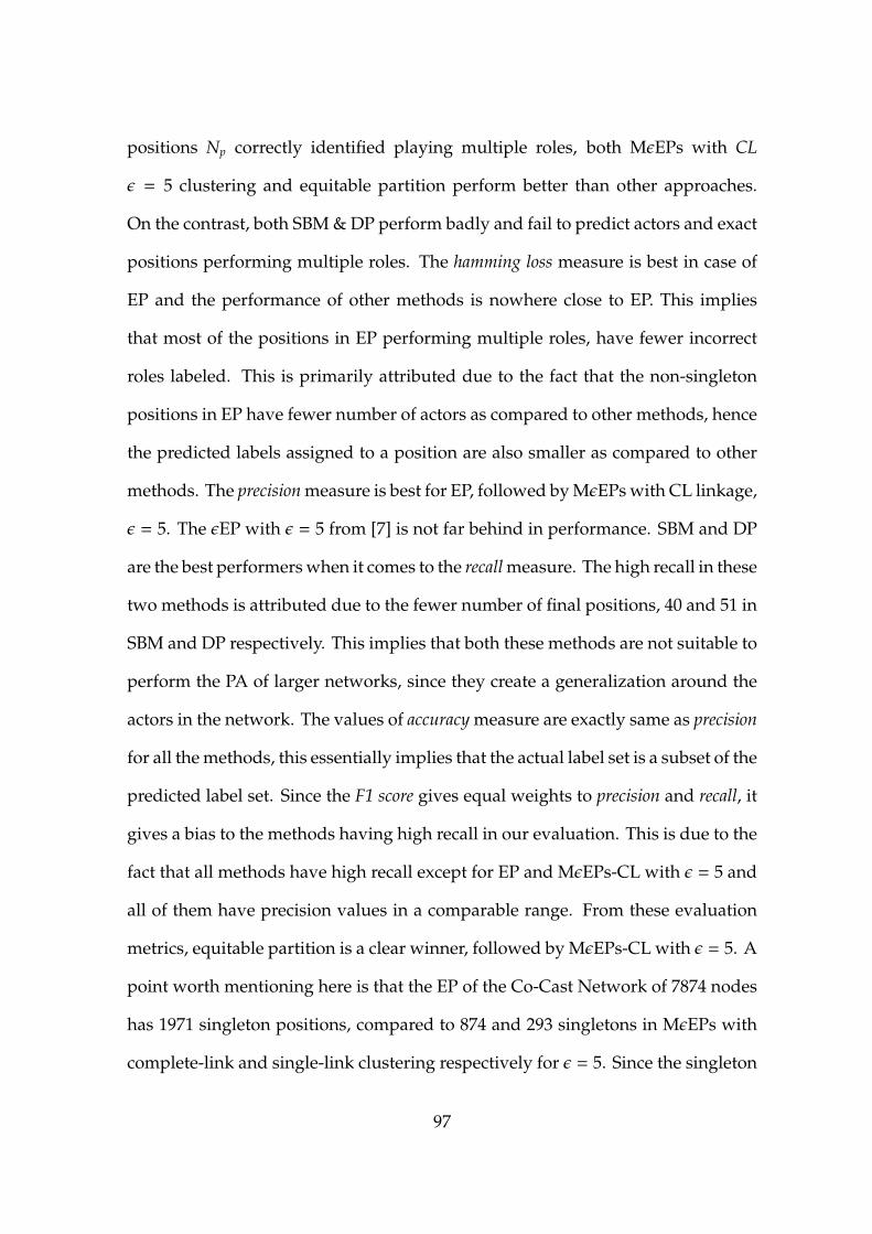
positions Np correctly identified playing multiple roles, both MεEPs with CL

ε = 5 clustering and equitable partition perform better than other approaches.

On the contrast, both SBM & DP perform badly and fail to predict actors and exact

positions performing multiple roles. The hamming loss measure is best in case of

EP and the performance of other methods is nowhere close to EP. This implies

that most of the positions in EP performing multiple roles, have fewer incorrect

roles labeled. This is primarily attributed due to the fact that the non-singleton

positions in EP have fewer number of actors as compared to other methods, hence

the predicted labels assigned to a position are also smaller as compared to other

methods. The precision measure is best for EP, followed by MεEPs with CL linkage,

ε = 5. The εEP with ε = 5 from [7] is not far behind in performance. SBM and DP

are the best performers when it comes to the recall measure. The high recall in these

two methods is attributed due to the fewer number of final positions, 40 and 51 in

SBM and DP respectively. This implies that both these methods are not suitable to

perform the PA of larger networks, since they create a generalization around the

actors in the network. The values of accuracy measure are exactly same as precision

for all the methods, this essentially implies that the actual label set is a subset of the

predicted label set. Since the F1 score gives equal weights to precision and recall, it

gives a bias to the methods having high recall in our evaluation. This is due to the

fact that all methods have high recall except for EP and MεEPs-CL with ε = 5 and

all of them have precision values in a comparable range. From these evaluation

metrics, equitable partition is a clear winner, followed by MεEPs-CL with ε = 5. A

point worth mentioning here is that the EP of the Co-Cast Network of 7874 nodes

has 1971 singleton positions, compared to 874 and 293 singletons in MεEPs with

complete-link and single-link clustering respectively for ε = 5. Since the singleton

97

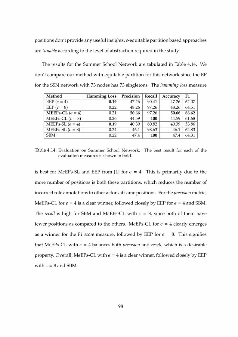
positions don’t provide any useful insights, ε-equitable partition based approaches

are tunable according to the level of abstraction required in the study.

The results for the Summer School Network are tabulated in Table 4.14. We

don’t compare our method with equitable partition for this network since the EP

for the SSN network with 73 nodes has 73 singletons. The hamming loss measure

Method Hamming Loss Precision Recall Accuracy F1EEP (ε = 4) 0.19 47.26 90.41 47.26 62.07EEP (ε = 8) 0.22 48.26 97.26 48.26 64.51MEEPs-CL (ε = 4) 0.21 50.66 97.26 50.66 66.62MEEPs-CL (ε = 8) 0.26 44.59 100 44.59 61.68MEEPs-SL (ε = 4) 0.19 40.39 80.82 40.39 53.86MEEPs-SL (ε = 8) 0.24 46.1 98.63 46.1 62.83SBM 0.22 47.4 100 47.4 64.31

Table 4.14: Evaluation on Summer School Network. The best result for each of theevaluation measures is shown in bold.

is best for MεEPs-SL and EEP from [1] for ε = 4. This is primarily due to the

more number of positions is both these partitions, which reduces the number of

incorrect role annotations to other actors at same positions. For the precision metric,

MεEPs-CL for ε = 4 is a clear winner, followed closely by EEP for ε = 4 and SBM.

The recall is high for SBM and MεEPs-CL with ε = 8, since both of them have

fewer positions as compared to the others. MεEPs-CL for ε = 4 clearly emerges

as a winner for the F1 score measure, followed by EEP for ε = 8. This signifies

that MεEPs-CL with ε = 4 balances both precision and recall, which is a desirable

property. Overall, MεEPs-CL with ε = 4 is a clear winner, followed closely by EEP

with ε = 8 and SBM.

98

Qualitative Analysis of Positions found using MεEPs for the Summer School

Network

We present a qualitative analysis of the roles found with MεEPs complete-link

linkage for ε = 4 on the SSN. Figure 4.8 shows the actor-actor distance matrix of

summer school network from MεEPs-CL with ε = 4. The 73 nodes of the distance

matrix are rearranged using the HAC complete-link linkage combination distance.

The red line on the dendrogram depicts the best clustering level as determined

by Algorithm 7. The red squares depict the 12 non-singleton clusters found at

this level of the dendrogram tree hierarchy. We interpret these clusters and show

how they correspond to the different roles of people that attended the event. The

interpretation of the clusters starting from the top left corner of the Figure 4.8 is as

follows:

(i) The first cluster having 4 people mostly comprising “attendee” Visitors of the

summer school, with an exception of a Local “attendee”. All members of this

cluster have moderate degrees. The dissimilarity of the Local with the Visitors

is evident in the Figure 4.8, the local corresponds to the left most element in

the plot.

(ii) The second cluster having 2 people who are “attendee” Visitors. Both have a

moderately low degree.

(iii) The third cluster having 3 members, two “attendee” Visitors and one “attendee”

Local. All members have moderate degrees. The local didn’t attend all

sessions actively, hence the connection pattern is more similar to visitors

who responded. The local is the left most element in the plot.

99

0 10 20 30 40 50 60 70

70

60

50

40

30

20

10

0

0.0

0.1

0.2

0.3

0.4

0.5

0.6

0.7

0.8

0.9

1.0

Figure 4.8: Heatmap of Actor-Actor Distance Matrix of Summer School Network fromMεEPs-CL with ε = 4. The 73 nodes of the distance matrix are rearrangedusing the HAC with complete-link combination distance. The correspondingdendrogram is shown at the top of the figure. The red line on the dendrogramdepicts the best clustering level as determined by Algorithm 7. The red squaresdepict the 12 non-singleton clusters found at this level of the dendrogram treehierarchy. We present the qualitative analysis of these 12 positions.

100

(iv) The fourth cluster having 3 members, two “attendee” Visitors and one “attendee”

Speaker (i.e., visiting speaker). All members have moderate degree of connections.

(v) The fifth cluster having 4 members, all of them being “attendee” Visitors. The

similarity among all the four members is visually evident in the plot.

(vi) The sixth cluster having 3 members, two of them are Senior “organizers”

and one of them is “attendee” Speaker. All members have high degree of

connections, consisting of people who interacted with most of the people

attending the summer school.

(vii) The seventh cluster having 3 members, one Senior “organizer”, one Local

“organizer” and one “attendee” Visitor. The members have moderately high

degrees. This implies that the senior organizer didn’t interact as much with

other people, as the other senior organizers did. The visitor interacted more as

compared to other visitors of the summer school. The dissimilarity between

the connection pattern of the senior organizer (left most in the cluster) is

evident in the plot.

(viii) The eighth cluster having 8 people. It has a mix of people in role of

Local “organizers” and “attendee” Visitors. The organizers were the “quiet”

ones, i.e., the people who didn’t respond to the summer school survey, but

interacted with most of the people. Hence they have moderate degree. The

visitors in this block were the people who also have moderate degree of

connections. The similarity among the locals is evident from the right most

members of the cluster in the figure.

(ix) The ninth cluster having 3 people. This block has two “attendee” Visitors and

101

one “attendee” Speaker. All of them were non-respondents.

(x) The tenth block having 2 people. These are the moderate degree organizers

similar to the seventh cluster, one of them being Senior and the other one

being Local. Dissimilarity in their role pattern is evident from the plot.

(xi) The eleventh cluster having 4 people. These are the Local “organizers” with

an exception of a Senior “organizer”. They have moderately high degree of

connections. The senior organizer has relatively less connections than other

people in the same role.

(xii) The twelfth block having 29 low degree nodes. This block has a mix of roles,

but predominantly having Visitors or Speakers who didn’t interact with other

people. This block also has 2 Senior Organizers who were also Speakers.

In the stochastic blockmodel [69] of the SSN, the authors identified 7 blocks.

We get a partition similarity score of 80% between the positions of this SBM

and the positions identified by our approach (MεEPs-CL, ε = 4). We get more

blocks primarily because, an epsilon value of 4 doesn’t combine blocks having

moderately-low and moderate degrees. Same applies for blocks having high

degrees and moderately-high degrees. The advantage with MεEPs is that, we

can tune epsilon to achieve granularity as required in the analysis.

Results of Dynamic Analysis

Results of Partition Similarity Score We perform the dynamic analysis as discussed

in the previous sections on the JMLR Co-Authorship & Co-Citation networks and

DBLP Co-Authorship network.

102

Table 4.15 to Table 4.20 tabulate the partition similarity score (Chapter 3, Equation

3.1) for each of the JMLR Co-citation network from year 2006 to 2011, for varying

values of ε = 2, 4, 6 found using MεEPs with complete-link and single-link clustering.

The source network at time t is depicted in the row of the table. The column

corresponds to the evolved network at time t + δt. MεEPs with single-link

linkage consistently performs better than complete-link linkage. Partitioning with

higher values of ε correspond to higher partition similarity scores, as evident

from Tables 4.15, 4.16. This is due to fewer number of positions, which increases

the likelihood of overlap amongst positions. Partitioning with a small value of

ε = 2 as depicted in Tables 4.19, 4.20 gives partition similarity of at least 65%

for networks separated by an year. We also get a partition overlap of ˜50% even

when the networks are separated by 5 years, as evident from Table 4.20. A smaller

ε corresponds to more number of positions in the partition, hence we get less

number of overlapping positions. In summary, MεEPs is a useful approach for

studying evolution of positions across time, we got a partition similarity as high

as 96% for the Co-Citation network separated by an year in time.

The comparison of various techniques of positional analysis for the partition

similarity score is depicted in Figure 4.9. The figure shows the partition similarity

score of year 2006 co-citation network with networks from years 2007 → 2011.

MεEPs-SL is a clear winner followed closely by SBM [69], MεEPs-CL and εEP [1].

DP and EP perform badly as the number of years start increasing, with EP having

0% partition overlap after year 2007.

103

2007 2008 2009 2010 2011Evolution of Co-Citation Network from Year 2006 with Year --->

0

10

20

30

40

50

60

70

80

90

Part

ition

Sim

ilarit

y (p

erce

ntag

e) --

->Partition Similarity for various Positional Analysis techniques, JMLR Co-Citation Network

MEEPs-CL-2MEEPs-SL-2

EEP2Degree

SBMEquitable

Figure 4.9: Comparison of Partition Similarity Score for JMLR Co-Citation Network usingvarious Positional Analysis methods. Source network is year 2006 Co-Citationnetwork, compared with networks from years 2007→ 2011.

Source Network 2007 2008 2009 2010 20112006 92.27 87.17 84.86 84.46 88.092007 93.31 90.8 88.13 91.752008 93.1 90.39 92.472009 92.7 91.292010 94.48

Table 4.15: Evolution in JMLR Co-Citation Network with MεEPs SL Epsilon=6

Source Network 2007 2008 2009 2010 20112006 77.48 68.78 65.7 67.24 62.272007 78.52 74.4 73.24 69.652008 80.61 78.52 75.462009 82.33 76.642010 83.34

Table 4.16: Evolution in JMLR Co-Citation Network with MεEPs CL Epsilon=6

104

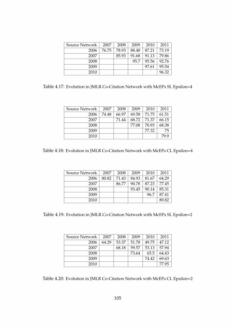
Source Network 2007 2008 2009 2010 20112006 76.75 78.93 88.48 87.21 73.192007 85.93 91.68 91.13 79.862008 95.7 95.56 92.762009 97.61 95.542010 96.32

Table 4.17: Evolution in JMLR Co-Citation Network with MεEPs SL Epsilon=4

Source Network 2007 2008 2009 2010 20112006 74.48 66.97 69.58 71.75 61.512007 71.44 68.72 71.37 66.152008 77.08 70.93 68.382009 77.32 752010 79.9

Table 4.18: Evolution in JMLR Co-Citation Network with MεEPs CL Epsilon=4

Source Network 2007 2008 2009 2010 20112006 80.82 71.43 84.93 81.67 64.292007 86.77 90.78 87.23 77.452008 93.45 90.14 85.312009 96.7 87.412010 89.82

Table 4.19: Evolution in JMLR Co-Citation Network with MεEPs SL Epsilon=2

Source Network 2007 2008 2009 2010 20112006 64.29 53.37 51.78 49.75 47.122007 68.18 59.57 53.13 57.942008 73.64 65.5 64.432009 74.42 69.632010 77.95

Table 4.20: Evolution in JMLR Co-Citation Network with MεEPs CL Epsilon=2

105

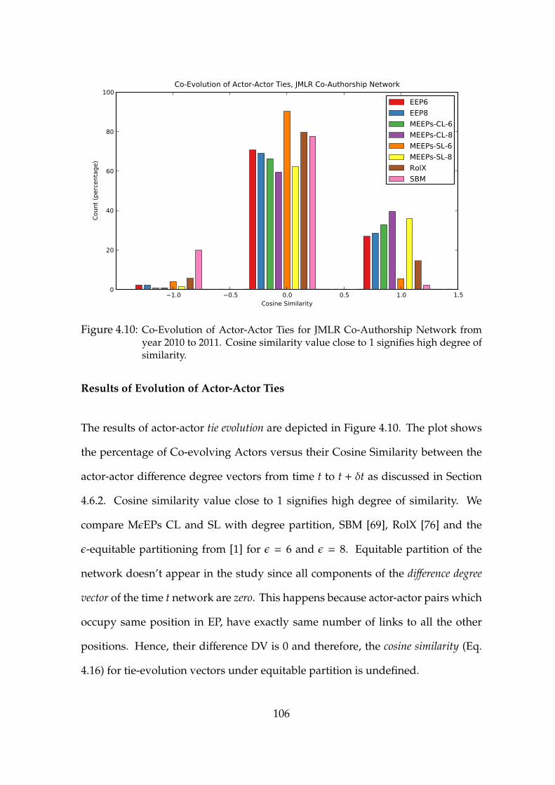
1.0 0.5 0.0 0.5 1.0 1.5Cosine Similarity

0

20

40

60

80

100Co

unt (

perc

enta

ge)

Co-Evolution of Actor-Actor Ties, JMLR Co-Authorship Network

EEP6EEP8MEEPs-CL-6MEEPs-CL-8MEEPs-SL-6MEEPs-SL-8RolXSBM

Figure 4.10: Co-Evolution of Actor-Actor Ties for JMLR Co-Authorship Network fromyear 2010 to 2011. Cosine similarity value close to 1 signifies high degree ofsimilarity.

Results of Evolution of Actor-Actor Ties

The results of actor-actor tie evolution are depicted in Figure 4.10. The plot shows

the percentage of Co-evolving Actors versus their Cosine Similarity between the

actor-actor difference degree vectors from time t to t + δt as discussed in Section

4.6.2. Cosine similarity value close to 1 signifies high degree of similarity. We

compare MεEPs CL and SL with degree partition, SBM [69], RolX [76] and the

ε-equitable partitioning from [1] for ε = 6 and ε = 8. Equitable partition of the

network doesn’t appear in the study since all components of the difference degree

vector of the time t network are zero. This happens because actor-actor pairs which

occupy same position in EP, have exactly same number of links to all the other

positions. Hence, their difference DV is 0 and therefore, the cosine similarity (Eq.

4.16) for tie-evolution vectors under equitable partition is undefined.

106

As evident from Figure 4.10, close to 40% actor-pairs follow their interaction

patterns with same set of positions in the evolved network in MεEPs. This signifies

that a good number of actor-pairs, who add new collaboration links with time,

mostly add them to similar social positions. The co-evolving actor-actor pairs

found using ε-equitable partition based approaches show tie evolution properties.

On the other hand, the co-evolving actors found using DP and SBM have tie

evolution difference degree vectors either independent or dissimilar to each other

as evident from the plot. RolX performs better than the previous two approaches,

but is no where close to εEP based methods. To conclude, MεEPs performed better

than all the other methods and successfully captured the co-evolution of node

ties/links to other positions. The significance of tie evolution characteristics of our

method can be easily used in link recommendation systems.

Results on Study of Network Centric properties for Co-Evolving Actor Pairs

We study the evolution of various graph theoretic network centric properties for

co-evolving actor-pairs of the DBLP Co-Authorship network. The evaluation

methodology is same as discussed in Chapter 3, Section 3.4.3. Figure 4.11 shows

the results. The x-axis corresponds to the bins containing the difference of a network

centric property. The y-axis corresponds to the frequency of node pairs that belong

to a particular bin, as a percentage of the total number of node pairs that occupy

the same position in the partition. EP outperforms all the other methods, followed

closely by MεEPs-CL clustering for ε = 2. SBM is the worst performer of all the

methods for betweenness centrality and number of triangles (Figure 4.11 (a) and

(c)). The percentage counts of the closeness centrality (Figure 4.11 (b)) are more

107

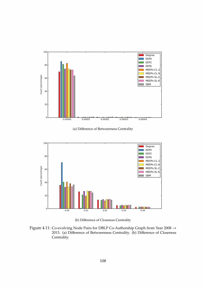
0.00000 0.00001 0.00002 0.00003 0.000040

20

40

60

80

100

Coun

t (pe

rcen

tage

)

DegreeEEP0EEP2EEP6MEEPs-CL-2MEEPs-CL-6MEEPs-SL-2MEEPs-SL-6SBM

(a) Difference of Betweenness Centrality

0.00 0.01 0.02 0.03 0.040

20

40

60

80

100

Coun

t (pe

rcen

tage

)

DegreeEEP0EEP2EEP6MEEPs-CL-2MEEPs-CL-6MEEPs-SL-2MEEPs-SL-6SBM

(b) Difference of Closeness Centrality

Figure 4.11: Co-evolving Node Pairs for DBLP Co-Authorship Graph from Year 2008→2013. (a) Difference of Betweenness Centrality. (b) Difference of ClosenessCentrality.

108

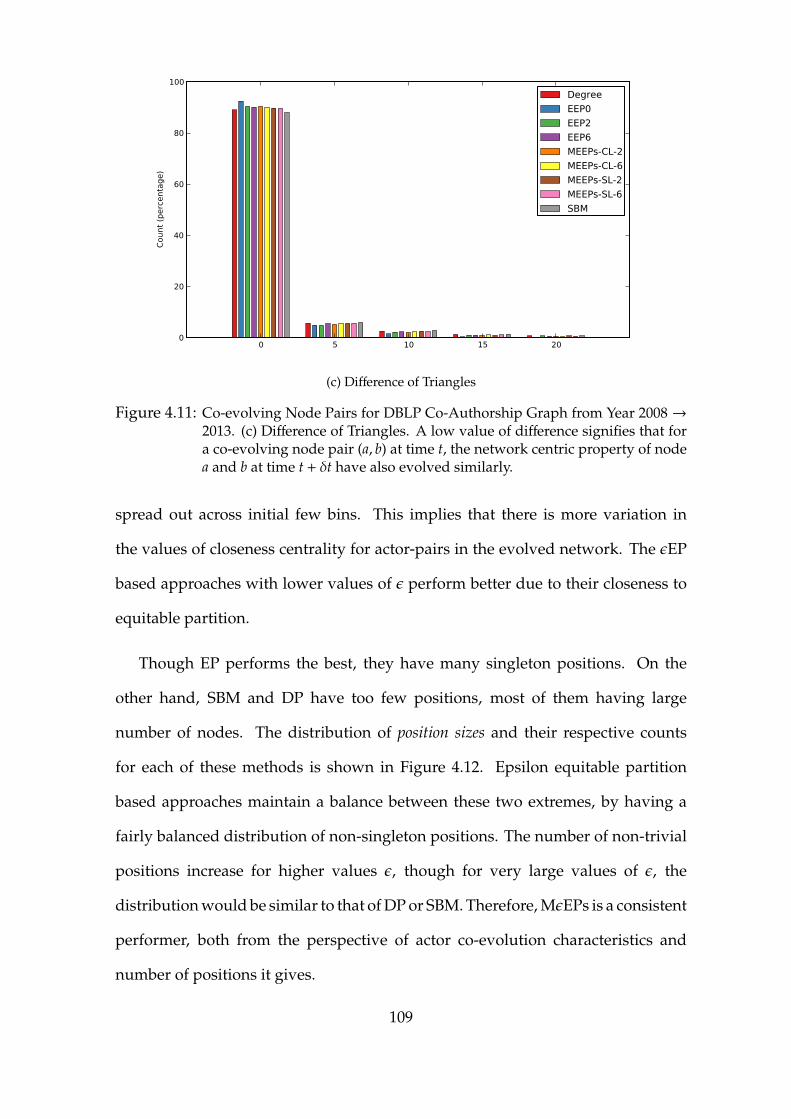
0 5 10 15 200

20

40

60

80

100

Coun

t (pe

rcen

tage

)

DegreeEEP0EEP2EEP6MEEPs-CL-2MEEPs-CL-6MEEPs-SL-2MEEPs-SL-6SBM

(c) Difference of Triangles

Figure 4.11: Co-evolving Node Pairs for DBLP Co-Authorship Graph from Year 2008→2013. (c) Difference of Triangles. A low value of difference signifies that fora co-evolving node pair (a, b) at time t, the network centric property of nodea and b at time t + δt have also evolved similarly.

spread out across initial few bins. This implies that there is more variation in

the values of closeness centrality for actor-pairs in the evolved network. The εEP

based approaches with lower values of ε perform better due to their closeness to

equitable partition.

Though EP performs the best, they have many singleton positions. On the

other hand, SBM and DP have too few positions, most of them having large

number of nodes. The distribution of position sizes and their respective counts

for each of these methods is shown in Figure 4.12. Epsilon equitable partition

based approaches maintain a balance between these two extremes, by having a

fairly balanced distribution of non-singleton positions. The number of non-trivial

positions increase for higher values ε, though for very large values of ε, the

distribution would be similar to that of DP or SBM. Therefore, MεEPs is a consistent

performer, both from the perspective of actor co-evolution characteristics and

number of positions it gives.

109

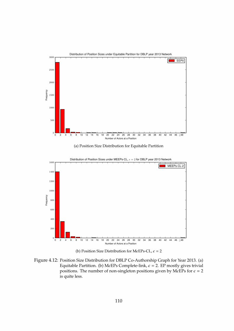
0 2 4 6 8 10 12 14 16 18 20 22 24 26 28 30 32 34 36 38 40 42 44 46 ≥48Number of Actors at a Position

0

500

1000

1500

2000

2500

3000

Freq

uenc

y

Distribution of Position Sizes under Equitable Partition for DBLP year 2013 Network

EEP0

(a) Position Size Distribution for Equitable Partition

0 2 4 6 8 10 12 14 16 18 20 22 24 26 28 30 32 34 36 38 40 42 44 46 ≥48Number of Actors at a Position

0

200

400

600

800

1000

1200

1400

1600

Freq

uenc

y

Distribution of Position Sizes under MEEPs-CL, ε = 2 for DBLP year 2013 Network

MEEPs-CL-2

(b) Position Size Distribution for MεEPs-CL, ε = 2

Figure 4.12: Position Size Distribution for DBLP Co-Authorship Graph for Year 2013. (a)Equitable Partition. (b) MεEPs Complete-link, ε = 2. EP mostly gives trivialpositions. The number of non-singleton positions given by MεEPs for ε = 2is quite less.

110

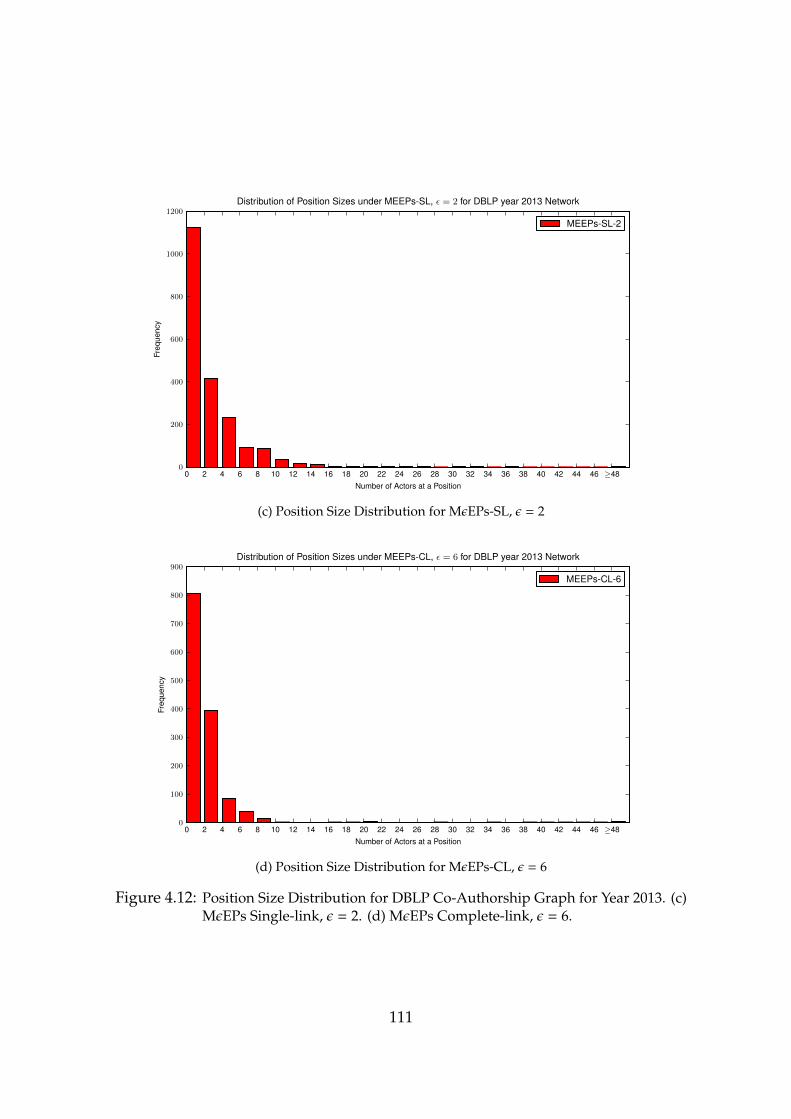
0 2 4 6 8 10 12 14 16 18 20 22 24 26 28 30 32 34 36 38 40 42 44 46 ≥48Number of Actors at a Position

0

200

400

600

800

1000

1200

Freq

uenc

y

Distribution of Position Sizes under MEEPs-SL, ε = 2 for DBLP year 2013 Network

MEEPs-SL-2

(c) Position Size Distribution for MεEPs-SL, ε = 2

0 2 4 6 8 10 12 14 16 18 20 22 24 26 28 30 32 34 36 38 40 42 44 46 ≥48Number of Actors at a Position

0

100

200

300

400

500

600

700

800

900

Freq

uenc

y

Distribution of Position Sizes under MEEPs-CL, ε = 6 for DBLP year 2013 Network

MEEPs-CL-6

(d) Position Size Distribution for MεEPs-CL, ε = 6

Figure 4.12: Position Size Distribution for DBLP Co-Authorship Graph for Year 2013. (c)MεEPs Single-link, ε = 2. (d) MεEPs Complete-link, ε = 6.

111

0 2 4 6 8 10 12 14 16 18 20 22 24 26 28 30 32 34 36 38 40 42 44 46 ≥48Number of Actors at a Position

0

100

200

300

400

500

600

700

Freq

uenc

y

Distribution of Position Sizes under MEEPs-SL, ε = 6 for DBLP year 2013 Network

MEEPs-SL-6

(e) Position Size Distribution for MεEPs-SL, ε = 6

0 2 4 6 8 10 12 14 16 18 20 22 24 26 28 30 32 34 36 38 40 42 44 46 ≥48Number of Actors at a Position

0

50

100

150

200

250

300

350

400

450

Freq

uenc

y

Distribution of Position Sizes under EEP, ε = 6 for DBLP year 2013 Network

EEP6

(f) Position Size Distribution for ε-Equitable Partition

Figure 4.12: Position Size Distribution for DBLP Co-Authorship Graph for Year 2013. (e)MεEPs Single-link, ε = 6. (f) εEP, ε = 6. Increasing the epsilon value, reducesthe number of non-trivial positions that we get using MεEPs, there is alsoa gradual increase in positions having lot of nodes, as evident from the lastbin.

112

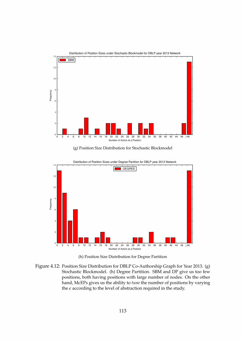
0 2 4 6 8 10 12 14 16 18 20 22 24 26 28 30 32 34 36 38 40 42 44 46 ≥48Number of Actors at a Position

0

2

4

6

8

10

12

14

Freq

uenc

yDistribution of Position Sizes under Stochastic Blockmodel for DBLP year 2013 Network

SBM

(g) Position Size Distribution for Stochastic Blockmodel

0 2 4 6 8 10 12 14 16 18 20 22 24 26 28 30 32 34 36 38 40 42 44 46 ≥48Number of Actors at a Position

0

2

4

6

8

10

12

14

Freq

uenc

y

Distribution of Position Sizes under Degree Partition for DBLP year 2013 Network

DEGREE

(h) Position Size Distribution for Degree Partition

Figure 4.12: Position Size Distribution for DBLP Co-Authorship Graph for Year 2013. (g)Stochastic Blockmodel. (h) Degree Partition. SBM and DP give us too fewpositions, both having positions with large number of nodes. On the otherhand, MεEPs gives us the ability to tune the number of positions by varyingthe ε according to the level of abstraction required in the study.

113

4.7 Conclusions and Discussion

We proposed a new notion of equivalence for discovering positions performing

multiple roles from a structural equivalence approach. The in-depth evaluation

of our proposed approach on real world ground-truth networks shows promising

results. Further, the results of our approach show that MεEPs is a promising tool

for studying the evolution of nodes and their ties in dynamic networks.

Discussion MεEPs closely resembles mixed membership stochastic blockmodels

(MMSB) [45] in spirit. In both these methods, an actor is allowed to occupy

multiple positions while allowing a bounded deviation from perfect equivalence.

The primary difference between these two methods is that our notion determines

equivalences purely from a structural equivalence aspect, whereas MMSB address

the same using probabilistic models.

The authors in [76] propose the notion of Role eXtraction (RolX).

RolX automatically determines the underlying roles in a network based on its

structural features. RolX is closely related to our work; the assignment of a node

to roles is mixed-membership. The authors demonstrate the advantage of their

role discovery approach in various mining tasks including transfer learning and

finding structural similarity.

114

CHAPTER 5

Conclusions and Future Work

5.1 Conclusions

In this thesis, we proposed ε-equitable partition based approaches (i) for scalable

positional analysis, and (ii) for discovering positions performing multiple roles.

We summarize our work as follows:

1. To the best of our knowledge, this is the first attempt at doing positional

analysis on a large scale online social network dataset. We have been able to

compute εEP for a significantly large component of the Flickr social graph

using our Parallel εEP Algorithm.

2. We proposed a new notion of equivalence for discovering positions performing

multiple roles from a structural equivalence approach. The evaluation of our

proposed MεEPs approach on real world multi-role ground truth networks

show promising results.

3. The results of both our proposed approaches show that εEP and MεEPs are

promising tools for studying the evolution of nodes and their ties in time

evolving networks.

We also presented efficient implementation for both the proposed methods.

The summary is as follows:

1. For the scalable ε-equitable partition algorithm we implemented a Lightweight

MapReduce framework using open source tools, which gave us millisecond

guarantees across iterative MapReduce steps. Further, this implementation

exploits data locality by intelligently partitioning the graph data across computing

nodes.

2. For the multiple ε-equitable partitions algorithm, we achieved parallelism

in computing these multiple εEPs by using a common shared instance of

vertex degree vectors of the graph and cell mapping files. This implementation

significantly reduced (i) the memory footprint, due to use of shared objects

and (ii) execution time, since re-computation of degree vectors was no longer

needed for the computation of the next ε-equitable partition.

5.2 Future Scope of Work

5.2.1 Structural Partitioning of Weighted Graphs

The definition ε-equitable partition applies to undirected simple graphs. Since

real world networks can be directed, weighted, and multi-relational, it would be

interesting to extend our definition to these classes of graphs.

The notion of edge-weight in a social network graph can be used to represent the

strength of social tie between two people. For example, an edge connecting user a

and user b may carry more weight than the edge connecting user a and user c, since

116

1 2 2 1 2 2

3 3

1 2 3 4 5 6

7 8

9

Figure 5.1: Example edge-weighted graph. The corresponding weighted equitable partitionis [{1,4},{2,3,5,6},{7,8},{9}]

a and b interact daily on a social network as opposed to one or two interactions

a month for the latter case. In this section, we present research directions on the

notion of equitable partition and ε-equitable partition for weighted graphs. We define

them as follows:

Definition 5.1. (weighted equitable partition) A partitionπ = {c1, c2, ..., cn}on edge-weighted

graph G ≡ 〈V,E〉, where V is the vertex set and E is the edge set is said to be weighted

equitable if,

for all 1 ≤ i, j ≤ n, strength(u, c j) = strength(v, c j) for all u, v ∈ ci (5.1)

where,

strength(vi, c j) = {Σw(vi, vk) | (vi, vk) ∈ E and vk ∈ c j} (5.2)

where, w(vi, vk) denotes the edge-weight of the edge (vi, vk) ∈ E. The term strength(vi, c j)

denotes the sum of edge-weights of vertices in cell c j adjacent to the vertex vi. Here,

cell c j denotes a position and therefore strength(vi, c j) means the strength actor vi

has to the position c j. Example weighted equitable partition is shown in Figure 5.1.

117

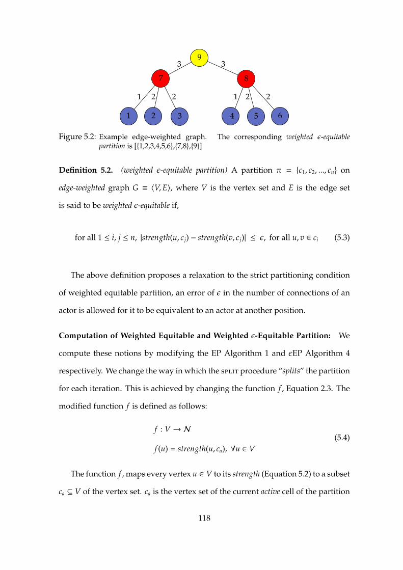
1 2 2 1 2 2

3 3

1 2 3 4 5 6

7 8

9

Figure 5.2: Example edge-weighted graph. The corresponding weighted ε-equitablepartition is [{1,2,3,4,5,6},{7,8},{9}]

Definition 5.2. (weighted ε-equitable partition) A partition π = {c1, c2, ..., cn} on

edge-weighted graph G ≡ 〈V,E〉, where V is the vertex set and E is the edge set

is said to be weighted ε-equitable if,

for all 1 ≤ i, j ≤ n, |strength(u, c j) − strength(v, c j)| ≤ ε, for all u, v ∈ ci (5.3)

The above definition proposes a relaxation to the strict partitioning condition

of weighted equitable partition, an error of ε in the number of connections of an

actor is allowed for it to be equivalent to an actor at another position.

Computation of Weighted Equitable and Weighted ε-Equitable Partition: We

compute these notions by modifying the EP Algorithm 1 and εEP Algorithm 4

respectively. We change the way in which the split procedure “splits” the partition

for each iteration. This is achieved by changing the function f , Equation 2.3. The

modified function f is defined as follows:

f : V →N

f (u) = strength(u, ca), ∀u ∈ V(5.4)

The function f , maps every vertex u ∈ V to its strength (Equation 5.2) to a subset

ca ⊆ V of the vertex set. ca is the vertex set of the current active cell of the partition

118

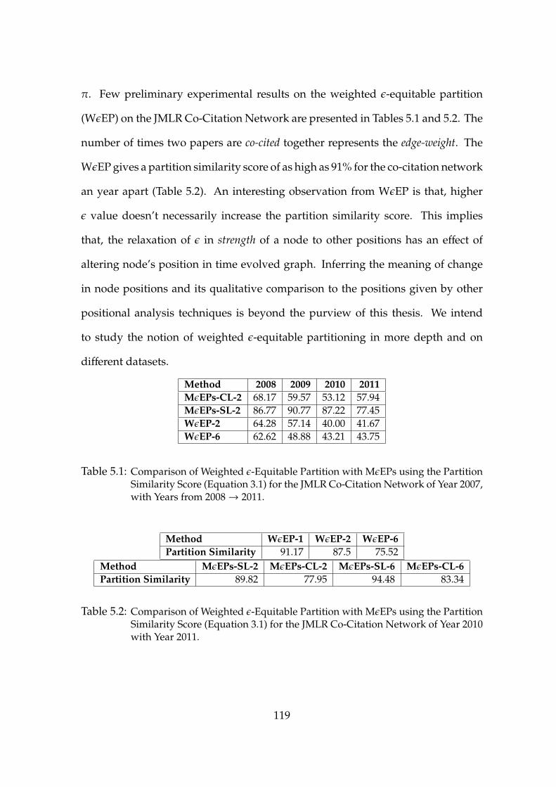
π. Few preliminary experimental results on the weighted ε-equitable partition

(WεEP) on the JMLR Co-Citation Network are presented in Tables 5.1 and 5.2. The

number of times two papers are co-cited together represents the edge-weight. The

WεEP gives a partition similarity score of as high as 91% for the co-citation network

an year apart (Table 5.2). An interesting observation from WεEP is that, higher

ε value doesn’t necessarily increase the partition similarity score. This implies

that, the relaxation of ε in strength of a node to other positions has an effect of

altering node’s position in time evolved graph. Inferring the meaning of change

in node positions and its qualitative comparison to the positions given by other

positional analysis techniques is beyond the purview of this thesis. We intend

to study the notion of weighted ε-equitable partitioning in more depth and on

different datasets.

Method 2008 2009 2010 2011MεEPs-CL-2 68.17 59.57 53.12 57.94MεEPs-SL-2 86.77 90.77 87.22 77.45WεEP-2 64.28 57.14 40.00 41.67WεEP-6 62.62 48.88 43.21 43.75

Table 5.1: Comparison of Weighted ε-Equitable Partition with MεEPs using the PartitionSimilarity Score (Equation 3.1) for the JMLR Co-Citation Network of Year 2007,with Years from 2008→ 2011.

Method WεEP-1 WεEP-2 WεEP-6Partition Similarity 91.17 87.5 75.52

Method MεEPs-SL-2 MεEPs-CL-2 MεEPs-SL-6 MεEPs-CL-6Partition Similarity 89.82 77.95 94.48 83.34

Table 5.2: Comparison of Weighted ε-Equitable Partition with MεEPs using the PartitionSimilarity Score (Equation 3.1) for the JMLR Co-Citation Network of Year 2010with Year 2011.

119

5.2.2 Scalable Equitable Partitioning

In future, it would be interesting to explore the implied advantage of our Parallel

εEP Algorithm to find the coarsest equitable partition of very large graphs for an ε = 0.

Finding the equitable partition of a graph forms an important intermediate stage in

all the practical graph automorphism finding softwares [38, 39]. Another possible

research direction is to explore algorithms for positional analysis of very large

graphs using vertex-centric computation paradigms such as Pregel and GraphChi

[77, 78].

120

APPENDIX A

Partition Similarity Score

In this appendix, we give a detailed note on the partition similarity score (Equation

3.1). We have used this as an evaluation measure to compare two partitions.

A.1 Mathematical Preliminaries

This section briefs out few mathematical preliminaries, which form the basis for

our partition similarity score.

Given, graph G≡ 〈V, E〉, V is the vertex set, E is the edge set andπ = {c1, c2, ..., cK}

is a partition of V. We define the following for any two partitions of a graph G ≡ 〈V,

E〉:

(i) Two partitions π1 and π2 are equal, iff they both partition the vertex set V of

G exactly in the same way of each other.

Example,

let, π1 = {{v1, v2, v3, v4}, {v5, v6}, {v7}, {v8, v9, v10}}

π2 = {{v6, v5}, {v3, v2, v4, v1}, {v9, v8, v10}, {v7}}.

then, π1 = π2

i.e. the order of cells in partition and the order of vertices inside a cell is not

important.

(ii) We define the intersection of two partitionsπ1 and π2, as a partition containing

the cells obtained from the set intersection operator applied cell-wise to member

cells of πε1 and πε2 (discarding the empty sets).

Example,

let, π1 = {{v1, v2, v3}, {v4, v5}, {v6, v7, v8}} and

π2 = {{v1, v2}, {v3, v4, v5}, {v6, v7}, {v8}}.

then, π1 ∩ π2 = {{v1, v2}, {v3}, {v4, v5}, {v6, v7}, {v8}}

(iii) Two partitions π1 and π2 are dissimilar, iff their intersection leads to a discrete

partition. A discrete partition is a one with only singleton cells.

Example,

let, π1 = {{v1, v2, v3}, {v4, v5}} and

π2 = {{v1, v4}, {v3, v5}, {v2}}.

then, π1 ∩ π2 = {{v1}, {v2}, {v3}, {v4}, {v5}}

Here, π1 ∩ π2 gives a discrete partition.

122

A.2 Simplified Representation of the Partition Similarity

Score

Equation 3.1 can be represented in a simplified form as follows:

sim(π1, π2)

=12

[(N − |π1 ∩ π2|

N − |π1|

)+

(N − |π1 ∩ π2|

N − |π2|

)]=

12

(1 −|π1 ∩ π2|

N

)[( 1

1 − |π1|

N

)+

( 1

1 − |π2|

N

)]=

12

C(π1 ∩ π2)[ 1C(π1)

+1

C(π2)

]=

C(π1 ∩ π2)H(C(π1),C(π2))

(A.1)

where,

C(π) =(1 − |π|N

),

|π| = cardinality of π,

N = cardinality of the discrete partition of π,

H(x, y) = harmonic mean of x and y.

The authors in [79] survey and compare several notions of distance indices

between partitions on the same set, which are available in the literature.

123

A.3 MapReduce Algorithm to Compute the Partition

Similarity Score

The partition similarity score of Equation 3.1 requires the cardinality of the

intersection set of the two partitions π1 and π2. Finding the intersection of two

partitions as per the definition of intersection from (ii), Appendix A.1 is O(n2)

operation, where n being the total number of vertices in the partition. Computing

this for very large graphs becomes intractable. To counter this problem, we provide

an algorithm based on the MapReduce paradigm [10] to compute the size of the

intersection set of π1 and π2 (i.e., |π1∩π2|). The algorithm is presented in Algorithm

box 8. The algorithm initializes by enumerating the indices of π2 for each cell index

of partition π1. For each key from this tuple, the map operation checks if these

two cells intersect or not. The map emits a value of 1 corresponding to a constant

key. The reduce operations computes the sum of these individual 1s. This sum

corresponds to |π1 ∩ π2|, which is used to compute the partition similarity score

from Equation 3.1.

A note on Algorithm 8: The initializemethod of Algorithm 8 (line 3), primarily

involves replicating/enumerating the cell indices of π2 to all the cell indices of

π1. Since cross operations are computationally very costly, the tractability of the

Algorithm is inherently dependent on ability to generate the cross product set of the

cell index tuples of the two input partitions.

124

Algorithm 8 MapReduce Partitions Intersection Set CardinalityInput: Partitionsπ1 andπ2. Letπ1={cell1:[v1, v2], cell2:[v3, v4, v5], ..., cellK:[vn−2, vn−1, vn]}and π2={cell1:[v1, v2, v3], cell2:[v4, v5], ..., cellL:[vn−1, vn]}Output: Partitions intersection set cardinality |π1 ∩ π2|

1: class Mapper2: tupleList enumCells=[ ]

3: method initialize()4: for each cell index i of π1 (i.e. 1 → K) enumerate the cell index j of π2 (i.e.

1→ L) do5: add tuple(i, j) to enumCells

6: method map(id t, tuple (i, j))7: intersect← {π1(i) ∩ π2( j)} . Appendix A.1, (ii)8: if intersect , φ then9: emit(id intersect, 1) . If the two cells have a overlap, emit value 1

corresponding to a constant key “intersect”

1: class Reducer2: method reduce(id key, values)3: sum = 04: for value in values5: sum = sum + value6: emit(key, sum) . |π1 ∩ π2|

125

REFERENCES

[1] K. Kate, “Positional Analysis of Social Networks,” Master of Technology Thesis Report,Department of Computer Science and Engineering, IIT Madras, 2009.

[2] F. Lorrain and H. White, “Structural Equivalence of Individuals in Social Networks,”Journal of Mathematical Sociology, vol. 1, no. 1, pp. 49–80, 1971.

[3] D. R. White and K. Reitz, “Graph and Semigroup Homomorphisms on Semigroupsof Relations,” Social Networks, vol. 5, pp. 193–234, 1983.

[4] M. G. Everett, “Role Similarity and Complexity in Social Networks,”Social Networks, vol. 7, no. 4, pp. 353 – 359, 1985. [Online]. Available:http://www.sciencedirect.com/science/article/pii/0378873385900139

[5] B. D. McKay, “Practical Graph Isomorphism,” Congressus Numerantium, vol. 30, pp.45–87, 1981.

[6] M. G. Everett and S. P. Borgatti, “Exact colorations of graphs and digraphs,”Social Networks, vol. 18, no. 4, pp. 319 – 331, 1996. [Online]. Available:http://www.sciencedirect.com/science/article/pii/0378873395002863

[7] K. Kate and B. Ravindran, “Epsilon Equitable Partition: A Positional Analysis methodfor Large Social Networks,” in In the Proceedings of 15th International Conference onManagement of Data (COMAD), 2009.

[8] A. Cardon and M. Crochemore, “Partitioning a Graph in O(|A|log2|V|),” TheoreticalComputer Science, vol. 19, pp. 85–98, 1982.

[9] R. Paige and R. E. Tarjan, “Three Partition Refinement Algorithms,” SIAM Journal onComputing, vol. 16, no. 6, pp. 973–989, 1987.

[10] J. Dean and S. Ghemawat, “MapReduce: Simplified Data Processing on LargeClusters,” Communications of the Association for Computing Machinery, vol. 51, no. 1,pp. 107–113, 2008.

[11] S. Wasserman and K. Faust, Social Network Analysis: Methods and Applications.Cambridge University Press, 1994.

[12] S. Borgatti and M. Everett, “Notions of Position in Social Network Analysis,”Sociological Methodology, vol. 22, no. 1, pp. 1–35, 1992.

[13] J. Lerner, “Role Assignments,” in Network Analysis, ser. Lecture Notes in ComputerScience, U. Brandes and T. Erlebach, Eds. Springer Berlin / Heidelberg, 2005, vol.3418, pp. 216–252.

[14] P. Doreian, “Actor Network Utilities and Network Evolution,” Social Networks, vol. 28,pp. 137–164, 2006.

126

[15] S. Nadel, The Theory of Social Structure. Cohen & West, London, 1957.

[16] R. S. Burt, “Positions in Networks,” Social Forces, vol. 55, pp. 93–122, 1976.

[17] R. Breiger, S. Boorman, and P. Arabie, “An Algorithm for Clustering RelationalData with Applications to Social Network Analysis and Comparison withMultidimensional Scaling,” Journal of Mathematical Psychology, vol. 12, no. 3, pp.328–383, 1975.

[18] L. Sailer, “Structural Equivalence: Meaning and Definition, Computation andApplication,” Social Networks, vol. 1, no. 1, pp. 73–90, 1979.

[19] M. Marx and M. Masuch, “Regular Equivalence and Dynamic Logic,” Social Networks,vol. 25, no. 1, pp. 51–65, 2003.

[20] M. Everett and S. Borgatti, “Role Colouring a Graph,” Mathematical Social Sciences,vol. 21, no. 2, pp. 183–188, 1991.

[21] S. Borgatti and M. Everett, “Two Algorithms for Computing Regular Equivalence,”Social Networks, vol. 15, no. 4, pp. 361–376, 1993.

[22] M. Everett and S. Borgatti, “An Extension of Regular Colouring of Graphs to Digraphs,Networks and Hypergraphs,” Social Networks, vol. 15, no. 3, pp. 237–254, 1993.

[23] S. P. Borgatti and M. G. Everett, “The Class of All Regular Equivalences: AlgebraicStructure and Computation,” Social Networks, vol. 11, pp. 65–88, 1989.

[24] K. Faust, “Comparison of Methods for Positional Analysis: Structural and GeneralEquivalences,” Social Networks, vol. 10, no. 4, pp. 313–341, 1988.

[25] P. Doreian, “Measuring Regular Equivalence in Symmetric Structures,” SocialNetworks, vol. 9, no. 2, pp. 89–107, 1987.

[26] S. Borgatti, “A Comment on Doreian’s Regular Equivalence in Symmetric Structures,”Social Networks, vol. 10, no. 3, pp. 265–271, 1988.

[27] C. Winship and M. Mandel, “Roles and Positions: A Critique and Extension of TheBlockmodeling Approach,” Sociological methodology, vol. 1984, pp. 314–344, 1983.

[28] M. Everett and S. Borgatti, “Calculating Role Similarities: An Algorithm that HelpsDetermine the Orbits of a Graph,” Social networks, vol. 10, no. 1, pp. 77–91, 1988.

[29] V. Batagelj, P. Doreian, and A. Ferligoj, “An Optimizational Approach to RegularEquivalence,” Social Networks, vol. 14, no. 1, pp. 121–135, 1992.

[30] J. Boyd, “Social Semigroups,” George Mason University Press, Fairfax, VA, 1991.

[31] S. Kirkpatrick, C. Gelatt Jr, and M. Vecchi, “Optimization by Simulated Annealing,”Science, vol. 220, no. 4598, pp. 671–680, 1983.

[32] S. Borgatti, M. Everett, and L. Freeman, “Ucinet 6 for Windows: Software for SocialNetwork Analysis,” Analytic Technologies, Harvard, MA, 2012.

127

[33] F. Glover et al., “Tabu search-part I,” ORSA Journal on computing, vol. 1, no. 3, pp.190–206, 1989.

[34] F. Roberts and L. Sheng, “How Hard is it to Determine if a Graph has a 2-RoleAssignment?” Networks, vol. 37, no. 2, pp. 67–73, 2001.

[35] J. Boyd, “Finding and Testing Regular Equivalence,” Social networks, vol. 24, no. 4,pp. 315–331, 2002.

[36] B. Kernighan and S. Lin, “An Efficient Heuristic Procedure for Partitioning Graphs,”Bell System Technical Journal, vol. 49, no. 2, pp. 291–307, 1970.

[37] J. Boyd and K. Jonas, “Are Social Equivalences Ever Regular? Permutation and Exacttests,” Social networks, vol. 23, no. 2, pp. 87–123, 2001.

[38] B. McKay, “nauty User’s Guide (Version 2.4),” http://cs.anu.edu.au/ bdm/nauty/, 2009.

[39] P. T. Darga, K. A. Sakallah, and I. L. Markov, “Faster Symmetry Discovery usingSparsity of Symmetries,” in Proceedings of the 45th annual Design Automation Conference.ACM, 2008, pp. 149–154.

[40] S. E. Fienberg and S. S. Wasserman, “Categorical Data Analysis of Single SociometricRelations,” Sociological methodology, pp. 156–192, 1981.

[41] P. W. Holland, K. B. Laskey, and S. Leinhardt, “Stochastic Blockmodels: First steps,”Social networks, vol. 5, no. 2, pp. 109–137, 1983.

[42] S. Wasserman and C. Anderson, “Stochastic a posteriori Blockmodels: Constructionand Assessment,” Social Networks, vol. 9, no. 1, pp. 1–36, 1987.

[43] T. A. Snijders and K. Nowicki, “Estimation and Prediction for Stochastic Blockmodelsfor Graphs with Latent Block Structure,” Journal of Classification, vol. 14, no. 1, pp.75–100, 1997.

[44] A. Wolfe and D. Jensen, “Playing Multiple Roles: Discovering Overlapping Rolesin Social Networks,” in ICML-04 Workshop on Statistical Relational Learning and itsConnections to Other Fields, 2004.

[45] E. M. Airoldi, D. M. Blei, S. E. Fienberg, and E. P. Xing, “Mixed Membership StochasticBlockmodels,” Journal of Machine Learning Research, vol. 9, no. 1981-2014, p. 3, 2008.

[46] G. S. Pathak, “Delivering the Nation: The Dabbawalas of Mumbai,” South Asia:Journal of South Asian Studies, vol. 33, no. 2, pp. 235–257, 2010.

[47] D. Baindur and R. M. Macario, “Mumbai lunch box delivery system: A transferablebenchmark in urban logistics?” Research in Transportation Economics, 2012.

[48] M. Janakiram. (2011, November) Architecting for the Cloud: Demo and BestPractices. Accessed January 25, 2014. [Online]. Available: http://aws.amazon.com/apac/events/2011/11/15/awsevent-india/

[49] A. S. Foundation, “Apache Hadoop. Available: http://hadoop.apache.org/.Accessed January 6, 2014.” [Online]. Available: http://hadoop.apache.org/

128

[50] P. Mundkur, V. Tuulos, and J. Flatow, “Disco: A Computing Platform for Large-ScaleData Analytics,” in Proceedings of the 10th ACM SIGPLAN workshop on Erlang. ACM,2011, pp. 84–89.

[51] J. Ekanayake, H. Li, B. Zhang, T. Gunarathne, S.-H. Bae, J. Qiu, and G. Fox, “Twister:A Runtime for Iterative MapReduce,” in Proceedings of the 19th ACM InternationalSymposium on High Performance Distributed Computing. ACM, 2010, pp. 810–818.

[52] Y. Bu, B. Howe, M. Balazinska, and M. D. Ernst, “HaLoop: Efficient Iterative DataProcessing on Large Clusters,” Proceedings of the VLDB Endowment, vol. 3, no. 1-2, pp.285–296, 2010.

[53] M. Zaharia, M. Chowdhury, M. J. Franklin, S. Shenker, and I. Stoica, “Spark: ClusterComputing with Working Sets,” in Proceedings of the 2nd USENIX conference on Hottopics in cloud computing, 2010, pp. 10–10.

[54] O. Tange, “GNU Parallel - The Command-line Power Tool,” login: The USENIXMagazine, pp. 42–47, 2011.

[55] A. Tridgell and P. Mackerras, ““The rsync algorithm,”Australian NationalUniversity,” TR-CS-96-05, Tech. Rep., 1996.

[56] M. Zaharia, M. Chowdhury, T. Das, A. Dave, J. Ma, M. McCauley, M. J. Franklin,S. Shenker, and I. Stoica, “Resilient Distributed Datasets: A Fault-Tolerant Abstractionfor In-Memory Cluster Computing,” in Proceedings of the 9th USENIX conference onNetworked Systems Design and Implementation. USENIX Association, 2012, pp. 2–2.

[57] B. Viswanath, A. Mislove, M. Cha, and K. P. Gummadi, “On the Evolution of UserInteraction in Facebook,” in Proceedings of the 2nd ACM workshop on Online SocialNetworks. ACM, 2009, pp. 37–42.

[58] A. Mislove, H. Koppula, K. Gummadi, P. Druschel, and B. Bhattacharjee, “Growth ofthe flickr social network,” in Proceedings of the first workshop on Online social networks.ACM, 2008, pp. 25–30.

[59] S. Suri and S. Vassilvitskii, “Counting Triangles and the Curse of the Last Reducer,”in Proceedings of the 20th International Conference on World Wide Web. ACM, 2011, pp.607–614.

[60] T. Michalak, K. Aaditha, P. Szczepanski, B. Ravindran, and N. R. Jennings, “EfficientComputation of the Shapley Value for Game-Theoretic Network Centrality,” Journalof AI Research, vol. 46, pp. 607–650, 2013.

[61] A. Clauset, C. Shalizi, and M. Newman, “Power-law Distributions in Empirical Data,”SIAM review, vol. 51, no. 4, pp. 661–703, 2009.

[62] A.-L. Barabasi and E. Bonabeau, “Scale-Free Networks,” Scientific American, vol. 288,pp. 60–69.

[63] M. Folk, A. Cheng, and K. Yates, “Hdf5: A file format and I/O library for HighPerformance Computing Applications,” in Proceedings of Supercomputing, vol. 99, 1999.

[64] H. Group, “Hdf User’s Guide, Release 4.2.10, March 2014,” 2014.

129

[65] C. D. Manning, P. Raghavan, and H. Schutze, Introduction to Information Retrieval.Cambridge University Press, 2008, vol. 1.

[66] M. Ackerman and S. Ben-David, “Measures of Clustering Quality: A Working Set ofAxioms for Clustering,” in Proceedings of Neural Information Processing Systems (NIPS),2008, pp. 121–128.

[67] Q. H. Nguyen and V. J. Rayward-Smith, “Internal quality measures for clusteringin metric spaces,” International Journal of Business Intelligence and Data Mining, vol. 3,no. 1, pp. 4–29, 2008.

[68] “Internet Movie Database, http://www.imdb.com. Accessed February 10, 2014.”

[69] A. F. McDaid, T. B. Murphy, N. Friel, and N. J. Hurley, “Improved Bayesian inferencefor the stochastic block model with application to large networks,” ComputationalStatistics & Data Analysis, vol. 60, pp. 12–31, 2013.

[70] T. Reuters, “Web of Science,” New York: Thomson Reuters, 2012.

[71] S. Team, “Science of Science (Sci2) Tool. Indiana University and Scitech Strategies,”2009.

[72] M. Ley, “The DBLP Computer Science Bibliography: Evolution, Research issues,Perspectives,” in String Processing and Information Retrieval. Springer, 2002, pp. 1–10.

[73] G. Tsoumakas and I. Katakis, “Multi-label Classification: An Overview,” InternationalJournal of Data Warehousing and Mining (IJDWM), vol. 3, no. 3, pp. 1–13, 2007.

[74] R. E. Schapire and Y. Singer, “BoosTexter: A boosting-based system for textcategorization,” Machine learning, vol. 39, no. 2-3, pp. 135–168, 2000.

[75] S. Godbole and S. Sarawagi, “Discriminative Methods for Multi-labeledClassification,” in Advances in Knowledge Discovery and Data Mining. Springer, 2004,pp. 22–30.

[76] K. Henderson, B. Gallagher, T. Eliassi-Rad, H. Tong, S. Basu, L. Akoglu, D. Koutra,C. Faloutsos, and L. Li, “RolX: Structural Role Extraction & Mining in Large Graphs,”in Proceedings of the 18th ACM SIGKDD international conference on Knowledge discoveryand data mining. ACM, 2012, pp. 1231–1239.

[77] G. Malewicz, M. H. Austern, A. J. Bik, J. C. Dehnert, I. Horn, N. Leiser, andG. Czajkowski, “Pregel: A System for Large-scale Graph Processing,” in Proceedings ofthe 2010 ACM SIGMOD International Conference on Management of Data. ACM, 2010,pp. 135–146.

[78] A. Kyrola, G. Blelloch, and C. Guestrin, “GraphChi: Large-scale Graph Computationon just a PC,” in Proceedings of the 10th USENIX Symposium on Operating Systems Designand Implementation (OSDI), 2012, pp. 31–46.

[79] L. Denœud and A. Guenoche, “Comparison of distance indices between partitions,”in Data Science and Classification. Springer, 2006, pp. 21–28.

130

LIST OF PAPERS BASED ON THESIS

1. Gupte, P.V., Ravindran, B., “Multiple Epsilon Equitable Partitions - Roles and

Positional Analysis for Real World Networks,” At the XXXII Meeting of the

International Network for Social Network Analysis, Redondo Beach, USA, March

2012. (SUNBELT 2012).

2. Gupte, P.V., Ravindran, B., “Scalable Positional Analysis for Studying Evolution

of Nodes in Networks,” In SIAM Data Mining 2014 Workshop on Mining

Networks and Graphs: A Big Data Analytic Challenge, Philadelphia, USA, April

2014. (SDM MNG 2014).

3. Gupte, P.V., Ravindran, B., “Soft Roles in Large Networks,” Under Preparation.

131

General Test Committee

Advisor Dr. Balaraman Ravindran, Computer Science and Engg.

Members Dr. Krishna M. Sivalingam, Computer Science and Engg. (Chairperson)

Dr. David Koilpillai, Electrical Engg.

Dr. Sutanu Chakraborti, Computer Science and Engg.

132

RESUME

Name Pratik Vinay Gupte

Permanent Address 46/8, Nehru Nagar (East),UCO Bank Road,Bhilai 490020,Chhattisgarh

E-Mail pratik.gupte@gmail.com

Website http://randomsurfer.in

Education

M.S. by Research (CSE) Indian Institute of Technology Madras

B.E. with Honours (CSE) Bhilai Institute of Technology, Durg (2006)

133