PRAM ModelsAdvanced Algorithms & Data Structures

Lecture Theme 13

Prof. Dr. Th. OttmannSummer Semester 2006

2

• In the PRAM model, processors communicate by reading from and writing to the shared memory locations.

• The power of a PRAM depends on the kind of access to the shared memory locations.

Classification of the PRAM model

3

In every clock cycle,• In the Exclusive Read Exclusive

Write (EREW) PRAM, each memory location can be accessed only by one processor.

• In the Concurrent Read Exclusive Write (CREW) PRAM, multiple processor can read from the same memory location, but only one processor can write.

Classification of the PRAM model

4

• In the Concurrent Read Concurrent Write (CRCW) PRAM, multiple processor can read from or write to the same memory location.

Classification of the PRAM model

5

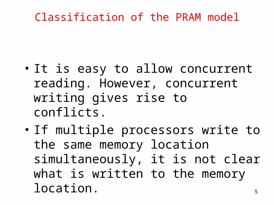
• It is easy to allow concurrent reading. However, concurrent writing gives rise to conflicts.

• If multiple processors write to the same memory location simultaneously, it is not clear what is written to the memory location.

Classification of the PRAM model

6

• In the Common CRCW PRAM, all the processors must write the same value.

• In the Arbitrary CRCW PRAM, one of the processors arbitrarily succeeds in writing.

• In the Priority CRCW PRAM, processors have priorities associated with them and the highest priority processor succeeds in writing.

Classification of the PRAM model

7

• The EREW PRAM is the weakest and the Priority CRCW PRAM is the strongest PRAM model.

• The relative powers of the different PRAM models are as follows.

Classification of the PRAM model

8

• An algorithm designed for a weaker model can be executed within the same time and work complexities on a stronger model.

Classification of the PRAM model

9

•We say model A is less powerful compared to model B if either:•the time complexity for solving a

problem is asymptotically less in model B as compared to model A. or,

•if the time complexities are the same, the processor or work complexity is asymptotically less in model B as compared to model A.

Classification of the PRAM model

10

An algorithm designed for a stronger PRAM model can be simulated on a weaker model either with asymptotically more processors (work) or with asymptotically more time.

Classification of the PRAM model

11

Adding n numbers on a PRAM

Adding n numbers on a PRAM

12

• This algorithm works on the EREW PRAM model as there are no read or write conflicts.

• We will use this algorithm to design a matrix multiplication algorithm on the EREW PRAM.

Adding n numbers on a PRAM

13

For simplicity, we assume that n = 2p for some integer p.

Matrix multiplication

14

• Each can be computed in parallel.

• We allocate n processors for computing ci,j. Suppose these processors are P1, P2,…,Pn.

• In the first time step, processor computes the product ai,m x bm,j.

• We have now n numbers and we use the addition algorithm to sum these n numbers in log n time.

, , 1 ,i jc i j n

, 1mP m n

Matrix multiplication

15

• Computing each takes n processors and log n time.

• Since there are n2 such ci,j s, we need overall O(n3) processors and O(log n) time.

• The processor requirement can be reduced to O(n3 / log n). Exercise !

• Hence, the work complexity is O(n3)

, , 1 ,i jc i j n

Matrix multiplication

16

• However, this algorithm requires concurrent read capability.

• Note that, each element ai,j (and bi,j) participates in computing n elements from the C matrix.

• Hence n different processors will try to read each ai,j (and bi,j) in our algorithm.

Matrix multiplication

17

For simplicity, we assume that n = 2p for some integer p.

Matrix multiplication

18

• Hence our algorithm runs on the CREW PRAM and we need to avoid the read conflicts to make it run on the EREW PRAM.

• We will create n copies of each of the elements ai,j (and bi,j). Then one copy can be used for computing each ci,j .

Matrix multiplication

19

Creating n copies of a number in O (log n) time using O (n) processors on the EREW PRAM.•In the first step, one processor reads

the number and creates a copy. Hence, there are two copies now.

•In the second step, two processors read these two copies and create four copies.

Matrix multiplication

20

•Since the number of copies doubles in every step, n copies are created in O(log n) steps.

•Though we need n processors, the processor requirement can be reduced to O (n / log n).Exercise !

Matrix multiplication

21

• Since there are n2 elements in the matrix A (and in B), we need O (n3 / log n) processors and O (log n) time to create n copies of each element.

• After this, there are no read conflicts in our algorithm. The overall matrix multiplication algorithm now take O (log n) time and O (n3 / log n) processors on the EREW PRAM.

Matrix multiplication

22

• The memory requirement is of course much higher for the EREW PRAM.

Matrix multiplication