
Practical Tractability of CSPs by Higher Level Consistency and Tree Decomposition Shant Karakashian...
46
Practical Tractability of CSPs by Higher Level Consistency and Tree Decomposition Shant Karakashian Dissertation Defense Collaborations: Bessiere, Geschwender, Hartke, Reeson, Scott, Woodward. Support: NSF CAREER Award #0133568 & NSF Grant No. RI-111795. Experiments were conducted on the equipment of the Holland Computing Center at UNL.
-
Upload
chaya-uttley -
Category
Documents
-
view
218 -
download
1
Transcript of Practical Tractability of CSPs by Higher Level Consistency and Tree Decomposition Shant Karakashian...
Practical Tractability of CSPs by Higher Level Consistency
and Tree Decomposition
Shant KarakashianDissertation Defense
Collaborations: Bessiere, Geschwender, Hartke, Reeson, Scott, Woodward.
Support: NSF CAREER Award #0133568 & NSF Grant No. RI-111795. Experiments were conducted on the equipment of the Holland Computing Center at UNL.

Karakashian: Ph.D. Defense 2
Context
• Constraint Satisfaction – General paradigm for modeling & solving
combinatorial decision problems– Applications in Engineering, Management,
Computer Science• Constraint Satisfaction Problems (CSPs) – NP-complete in general
• Islands of tractability– Classes of CSPs solvable in polynomial time
4/11/2013

Karakashian: Ph.D. Defense 3
Our Focus
• One tractability condition links [Freuder 82]– Consistency level to– Width of the constraint network, a structural parameter
(treewidth)• Catch 22– Computing width is in NP-hard– Enforcing higher-levels of consistency may require adding
constraints, which increases the treewidth• Goal– Exploit above condition to achieve practical tractability
4/11/2013

Karakashian: Ph.D. Defense 4
Our Approach
• Exploit a tree decomposition – Localize application of the consistency
algorithm– Steer constraint propagation along the
branches of the tree– Add redundant constraints at separators
to enhance propagation
4/11/2013
• Propose consistency properties that– Enforce a (parameterized) consistency level– While preserving the width of a problem instance
Karakashian: Ph.D. Defense 5
Outline
• Background• Contributions
– R( ,m)C: Consistency property & algorithms∗
[SAC 10, AAAI 10]
– Localized consistency & structure-guided propagation– Bolstering propagation at separators
[CP 12, AAAI 13]
– Counting solutions– (Appendices include other incidental contributions)
• Conclusions & Future Research4/11/2013
Background R(*,m)C Locallization Bolstering Sol Counting Conclusions

Karakashian: Ph.D. Defense 6
Constraint Satisfaction Problem (CSP)
• Given– A set of variables, here X={A,B,C,D,E,F,G}– Their domains, here D={DA,DB,DC,DD,DE,DF,DG}, Di={0,1}
– A set of constraints, here C={C1,C2,C3,C4,C5} where Ci = ⟨Ri,scope(Ri)⟩
• Question: Find one solution (NPC), find all solutions (#P)
R1
A E F0 0 10 1 00 1 11 0 11 1 0
R3
A B C0 0 10 1 00 1 11 0 11 1 0
R4
A D G0 0 10 1 00 1 11 0 11 1 0
R2
B E0 11 0
R5
B D0 11 0
4/11/2013
R4
R5R2R1
R3
GF A E B C D
A 0⟵B 0⟵C 1⟵D 1⟵E 1⟵F 0⟵G 0⟵
Background R(*,m)C Locallization Bolstering Sol Counting Conclusions
Karakashian: Ph.D. Defense 7
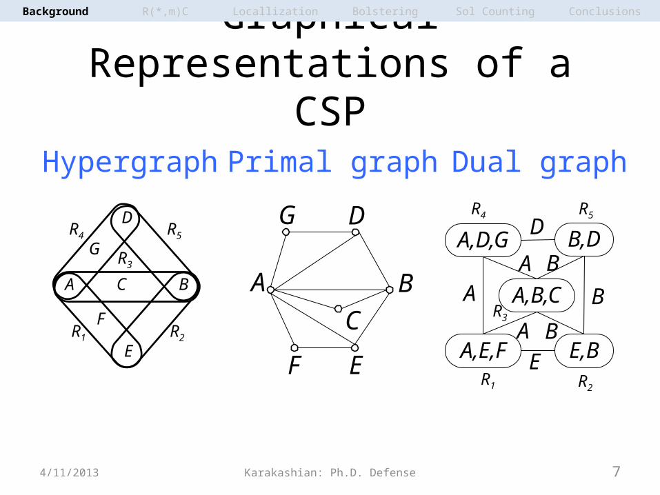
Graphical Representations of a CSP
Hypergraph Primal graph Dual graph
A BC
D
EF
G
A,B,C
A,E,F E,B
B,DA,D,G
A
A
A B
D
B
BE
A BC
D
E
F
GR4 R5
R2R1
R3
4/11/2013
R4 R5
R2R1
R3
Background R(*,m)C Locallization Bolstering Sol Counting Conclusions

Karakashian: Ph.D. Defense 8
Redundant Edges in a Dual Graph
• R1R4 forces the value of A in R1 and R4
• The value of A is enforced through R1R3 and R3R4
• R1R4 is redundant
4/11/2013
A,B,C
A,E,F E,B
B,DA,D,G
A
A
A B
D
B
B
E
R4 R5
R2R1
R3
Background R(*,m)C Locallization Bolstering Sol Counting Conclusions

Karakashian: Ph.D. Defense 9
Solving CSPs
• A CSP can be solved by– Search (conditioning)
• Backtrack search• Iterative repair (local search)
– Synthesizing & propagating constraints (inference)• Backtrack search – Constructive, exhaustive exploration of search space– Variable ordering improves the performance– Constraint propagation prunes the search tree
4/11/2013
Background R(*,m)C Locallization Bolstering Sol Counting Conclusions

Karakashian: Ph.D. Defense 10
Consistency Property: Definition
• Example: k-consistency requires that – For all combinations of k-1 variables
… all combinations of consistent values… can always be extended to every kth variable
• A consistency property– Guarantees that the values of all combinations of variables of a given
size verify some set of constraints – Is a necessary but not sufficient condition for partial solution to
appear in a complete solution
any consistent assignment of length k-1 kth variable
4/11/2013
Background R(*,m)C Locallization Bolstering Sol Counting Conclusions

Karakashian: Ph.D. Defense 11
Algorithms for Enforcing a Consistency Property
• May require adding new implicit or redundant constraints– For k-consistency: add constraints to eliminate inconsistent (k-1)-tuples
– Which may increase the width of the problem
• We propose a consistency property that– Never increases the width of the problem– Allows us to increase & control the level of consistency– Operates by deleting tuples from relations
any consistent assignment of length k-1 kth variable
4/11/2013
Background R(*,m)C Locallization Bolstering Sol Counting Conclusions

Karakashian: Ph.D. Defense 12
Tree Decomposition• A tree decomposition:⟨T, , 𝝌 𝜓⟩
– T: a tree of clusters– 𝝌: maps variables to clusters– 𝜓: maps constraints to clusters
{A,B,C,E} , {R2,R3}
{A,B,D},{R3,R5}{A,E,F},{R1}
{A,D,G},{R4}
C1
C2 C3
C4
Hypergraph Tree decomposition
• Conditions– Each constraint appears in at least
one cluster with all the variables in the constraint’s scope
– For every variable, the clusters where the variable appears induce a connected subtree
4/11/2013
A BC
D
E
F
GR4 R5
R2R1
R3
𝝌(C1) 𝜓(C1)
Background R(*,m)C Locallization Bolstering Sol Counting Conclusions

Karakashian: Ph.D. Defense 13
• A separator of two adjacent clusters is the set of variables associated to both clusters
• Width of a decomposition/network– Treewidth = maximum number of variables in clusters
Tree Decomposition: Separators
AB
C
D
E
F
G
C1
C2C3
C4
4/11/2013
{A,B,C,E},{R2,R3}
{A,B,D},{R3,R5}{A,E,F},{R1}
{A,D,G},{R4}
C1
C2 C3
C4
Background R(*,m)C Locallization Bolstering Sol Counting Conclusions

Karakashian: Ph.D. Defense 14
Outline
• Background• Contributions
– R( ,m)C: Consistency property & algorithms∗
[SAC 10, AAAI 10]
– Localized consistency & structure-guided propagation– Bolstering propagation at separators
[CP 12, AAAI 13]
– Counting solutions– (Appendices include other incidental contributions)
• Conclusions & Future Research4/11/2013
Background R(*,m)C Locallization Bolstering Sol Counting Conclusions

Karakashian: Ph.D. Defense 15
Relational Consistency R( ,m)C∗
4/11/2013
[SAC 2010, AAAI 2010]
• A parametrized relational consistency property• Definition
– For every set of m constraints– every tuple in a relation can be extended to an assignment– of variables in the scopes of the other m-1 relations
• R(*,m)C ≡ every m relations form a minimal CSP
R(*,m)C Locallization Bolstering Sol Counting ConclusionsBackground

Karakashian: Ph.D. Defense 16
Index-Tree Data Structure
• Given: two relations, R1 & R2
– Scope(R1)={X,A,B,C} Scope(R2)={A,B,C,D}
• For a given tuple in R1, find matching tuples in R2
4/11/2013
R2
A B C D deleted
t1 0 0 1 0 0
t2 0 1 1 0 0
t3 0 1 1 1 0
t4 1 1 1 1 0
0
0
1
1
1
1
1
1
t1 t2
t3
t4
A
B
C
Root
R(*,m)C Locallization Bolstering Sol Counting ConclusionsBackground

Karakashian: Ph.D. Defense 17
R1 R2 R3
R1 R2 R4
R1 R2 R5
R1 R3 R4
R2 R3 R4
R2 R4 R5
R3 R4 R5
• Weaken R( ,m)C by removing redundant edges∗
[Jégou 89]
Weakening R(∗,m)C
R1 R2 R3
R1 R2 R5
R1 R3 R4
R2 R4 R5
R3 R4 R5
CF
CG
AD
AE
ABD
ACEG
BCF
ADECFG
R1
R3
R2
R4
R5
A
B
CCF
CG
AD
AE
ABD
ACEG
BCF
ADECFG
R1
R3
R2
R4
R5
B
4/11/2013
R( ,3)C∗ wR( ,3)C∗
R(*,m)C Locallization Bolstering Sol Counting ConclusionsBackground

Karakashian: Ph.D. Defense 18
Characterizing R(∗,m)C
4/11/2013
GAC maxRPWC
R3C
R( ,2)C∗wR( ,2)C∗
R2C
R( ,3)C∗ R( ,4)C∗
R4C
wR( ,3)C∗ wR( ,4)C∗
R( ,∗ m)C
RmC
wR( ,∗ m)C
• GAC
[Waltz 75]
• maxRPWC
[Bessiere+ 08]
• RmC: Relational m Consistency
[Dechter+ 97]
[Jégou 89]
R(*,m)C Locallization Bolstering Sol Counting ConclusionsBackground

Karakashian: Ph.D. Defense 19
Empirical Evaluations (1)
4/11/2013
Algorithm Avg. #Nodes Avg. Time sec #Completed #Fastest #BF
SAT aim-100 (instances: 16, vars: 100, dom: 2, rels: 307, arity: 3)
GAC 9,459,773.0 759.7 15 4 1
wR( ,2)C∗ 234,526.7 125.6 16 7 5
wR( ,3)C∗ 3,979.1 19.4 16 3 7
wR( ,4)C∗ 559.1 26.32 16 2 9
SAT modifiedRenault (instances: 19, vars: 110, dom: 42, rels: 128, arity: 10)
GAC 1,171,458.43 108.5 17 14 5
wR( ,2)C∗ 211.5 4.98 19 5 7
wR( ,3)C∗ 110.4 13.3 19 0 14
wR( ,4)C∗ 110.2 81.3 19 0 16
R(*,m)C Locallization Bolstering Sol Counting ConclusionsBackground

Karakashian: Ph.D. Defense 20
Empirical Evaluations (2)
4/11/2013
Algorithm Avg. #Nodes Avg. Time sec #Completed #Fastest #BF
UNSAT aim-100 (instances: 8, vars: 100, dom: 2, rels: 173, arity: 3)
GAC - - 0 0 0
wR( ,2)C∗ 4,619,373.0 2,016.8 3 1 0
wR( ,3)C∗ 18,766.6 97.4 4 3 0
wR( ,4)C∗ 18,685.3 944.2 4 1 1
UNSAT modifiedRenault (instances: 31, vars: 111, dom: 42, rels: 130, arity: 10)
GAC 1,171,458.43 782.3 9 2 0
wR( ,2)C∗ 487.0 5.2 28 20 25
wR( ,3)C∗ 0.0 9.6 30 2 28
wR( ,4)C∗ 0.0 44.2 31 2 31
R(*,m)C Locallization Bolstering Sol Counting ConclusionsBackground

Karakashian: Ph.D. Defense 21
Algorithms for Enforcing R( ,m)C∗
• PERTUPLE– For each tuple find a solution for the variables in
the m-1 relations– Many satisfiability searches
• Effective when there are many solutions• Each search is quick & easy
• ALLSOL – Find all solutions of problem induced by m
relations, & keep their tuples– A single exhaustive search
• Effective when there are few or no solutions
• Hybrid Solvers (portfolio based) [+Scott]
4/11/2013
t1
ti
t2
t3
R(*,m)C Locallization Bolstering Sol Counting ConclusionsBackground
Karakashian: Ph.D. Defense 22
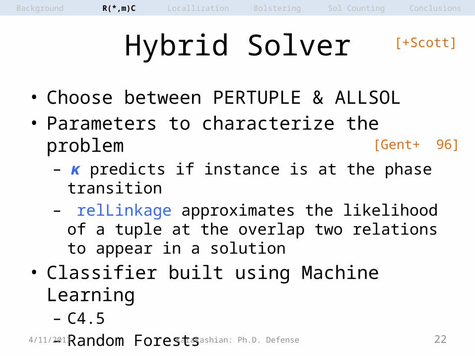
Hybrid Solver
• Choose between PERTUPLE & ALLSOL• Parameters to characterize the problem– κ predicts if instance is at the phase transition– relLinkage approximates the likelihood of a tuple at
the overlap two relations to appear in a solution
• Classifier built using Machine Learning– C4.5– Random Forests
4/11/2013
[+Scott]
[Gent+ 96]
R(*,m)C Locallization Bolstering Sol Counting ConclusionsBackground

Karakashian: Ph.D. Defense 23
Decision Tree
4/11/2013
#1≤ 0.22No
#3≤-2.79 No
#7≤0.03 No
#10≤10.05
Yes
No
#2≤-28.75
Yes
No
PERTUPLE
ALLSOLYes
YesPERTUPLE
Yes
ALLSOL
ALLSOL #7≤0.23 Yes No
ALLSOLPERTUPL
E
#1 κ
#2 log2(avg(relLinkage))
#3 log2(stDev(relLinkage))
#7
stDev(tupPerVvpNorm)
#10 avg(relPerVar)
R(*,m)C Locallization Bolstering Sol Counting ConclusionsBackground

Karakashian: Ph.D. Defense 24
Empirical Evaluations (3)
4/11/2013
#Instances solved by… Average CPU sec
Partition ALLSOL PERTUPLE
SOLVERC4
.5SOLVERRF#Instanc
es ALLSOL PERTUPLE
SOLVERC4.5
SOLVERRF
A 5,777 5,776 5,777 5,777 5,776 1.27 4.97 2.14 2.27
P 10,095 15,457 15,439 14,012 10,095 109.61 5.21 7.72 31.53
A ∪ P 15,872 21,333 21,216 19,789 15,871 70.18 5.12 5.69 20.88
Task: compute the minimal CSP
R(*,m)C Locallization Bolstering Sol Counting ConclusionsBackground
Karakashian: Ph.D. Defense 25
Outline
• Background• Contributions
– R( ,m)C: Consistency property & algorithms∗
[SAC 10, AAAI 10]
– Localized consistency & structure-guided propagation– Bolstering propagation at separators
[CP 12, AAAI 13]
– Counting solutions– (Appendices include other incidental contributions)
• Conclusions & Future Research4/11/2013
Locallization Bolstering Sol Counting ConclusionsBackground R(*,m)C
Karakashian: Ph.D. Defense 26
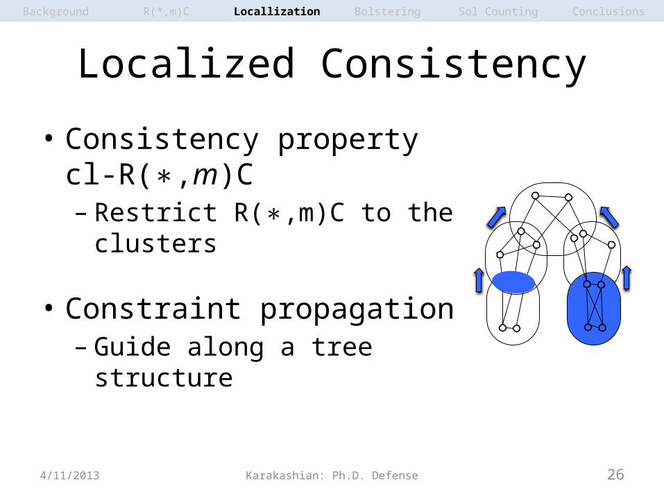
Localized Consistency
• Consistency property cl-R( ,∗ m)C– Restrict R( ,m)C to the clusters ∗
• Constraint propagation – Guide along a tree structure
4/11/2013
Locallization Bolstering Sol Counting ConclusionsBackground R(*,m)C

Karakashian: Ph.D. Defense 27
C1
C2
C7
C3
C4
C5C6
C8
C9C10
• Triangulate the primal graph using min-fill• Identify the maximal cliques using MAXCLIQUES• Connect the clusters using JOINTREE • Add constraints to clusters where their scopes appear
Generating a Tree Decomposition
4/11/2013
A B C
ED
FGH
I J K
M L
NR7
R2
R3
R4
R5
R6
R1
AB
C
E
D
F
G
HI
JK
M
L
N
C8
C2
A,B,C,N
A,I,N
B,C,D,H
I,M,N
B,D,F,H
C1
C3
C7
A,I,KC4
I,J,KC5
A,K,LC6
B,D,E,FC9
F,G,HC10 Elim
inati
on o
rder
MAXCLIQUES
{A,B,C,N},{R1}
C2 C7
C3 C8
C1
C4
C5 C6 C9 C10
JOINTREEmin-fill
Locallization Bolstering Sol Counting ConclusionsBackground R(*,m)C

Karakashian: Ph.D. Defense 28
Information Transfer Between Clusters
• Two clusters communicate via their separator– Constraints common to the two clusters– Domains of variables common to the two clusters
4/11/2013
E
R6 R5 R7
R4
R2 R1 R3
B A D C
F
Locallization Bolstering Sol Counting ConclusionsBackground R(*,m)C
R4A DB A D C

Karakashian: Ph.D. Defense 29
Characterizing cl-R( ,∗ m)C
4/11/2013
GAC
maxRPWC
R3C
R( ,2)C ≡∗wR( ,2)C∗
R2C
R( ,3)C∗ R( ,4)C∗
R4C
wR( ,3)C∗ wR( ,4)C∗
R( ,∗ m)C
RmC
wR( ,∗ m)C
cl-R( ,3)C∗cl-R( ,2)C∗ cl-R( ,4)C∗ cl-R( ,∗ m)C
cl-w( ,3)C∗cl-w( ,2)C∗ cl-w( ,∗ 4)C cl-w( ,∗ m)C
• GAC
[Waltz 75]
• maxRPWC
[Bessiere+ 08]
• RmC: Relational m Consistency
[Dechter+ 97]
Locallization Bolstering Sol Counting ConclusionsBackground R(*,m)C

Karakashian: Ph.D. Defense 30
Empirical Evaluations: Localization
4/11/2013
0.00014 0.014 1.4 140 140000.00014
0.014
1.4
140
14000
unsatsat
wR( ,3)C ∗
cl-w
R(,3
)C∗
Time (sec)
Tim
e (s
ec)
0.00014 0.014 1.4 140 140000.00014
0.014
1.4
140
14000
unsatsat
GACcl
-R(
,|ψ
(cli)
|)C
∗
Time (sec)
Tim
e (s
ec)
Locallization Bolstering Sol Counting ConclusionsBackground R(*,m)C
Karakashian: Ph.D. Defense 31
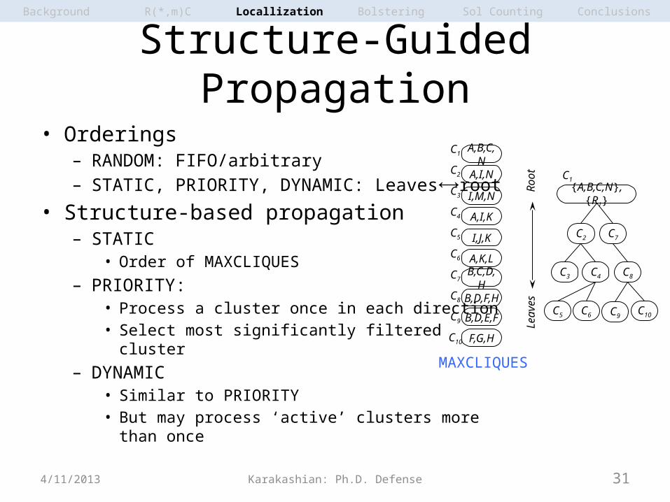
Structure-Guided Propagation
• Orderings– RANDOM: FIFO/arbitrary– STATIC, PRIORITY, DYNAMIC: Leaves root⟷
• Structure-based propagation– STATIC
• Order of MAXCLIQUES– PRIORITY:
• Process a cluster once in each direction• Select most significantly filtered cluster
– DYNAMIC• Similar to PRIORITY• But may process ‘active’ clusters more than once
4/11/2013
{A,B,C,N},{R1}
C2 C7
C3 C8
C1
C4
C5 C6 C9 C10
C8
C2
A,B,C,N
A,I,N
B,C,D,H
I,M,N
B,D,F,H
C1
C3
C7
A,I,KC4
I,J,KC5
A,K,LC6
B,D,E,FC9
F,G,HC10
Leav
esRo
ot
MAXCLIQUES
Locallization Bolstering Sol Counting ConclusionsBackground R(*,m)C

Karakashian: Ph.D. Defense 32
Empirical Evaluations: Propagation
4/11/2013
+ maxRPWC, m=2,4 cl-wR( ,3)C∗ cl-R( ,|∗ ψ(cl)|)C
#Instances RANDOM STATIC PRIORITY DYNAMIC RANDOM STATIC PRIORITY DYNAMIC
Completed
UNSAT 233 232 233 234 261 285 282 282
479 48.6% 48.4% 48.6% 48.9% 54.5% 59.5% 58.9% 58.9%
SAT 164 164 165 163 154 152 151 151
200 82.0% 82.0% 82.5% 81.5% 77.0% 76.0% 75.5% 75.5%
Fastest
UNSAT 66 157 117 114 151 220 161 155
479 13.8% 32.8% 24.4% 23.8% 31.5% 45.9% 33.6% 32.4%
SAT 51 88 111 108 50 88 74 84
200 25.5% 44.0% 55.5% 54.0% 25.0% 44.0% 37.0% 42.0%Avg. Time
(sec)
UNSAT Nbr instances 232 Nbr instances 254
479 402.9 383.9 366.3 369.3 397.4 318.9 341.3 344.1
SAT Nbr instances 162 Nbr instances 150
200 622.9 601.6 599.2 598.3 571.1 542.5 557.7 546.8
Locallization Bolstering Sol Counting ConclusionsBackground R(*,m)C

Karakashian: Ph.D. Defense 33
Outline
• Background• Contributions
– R( ,m)C: Consistency property & algorithms∗
[SAC 10, AAAI 10]
– Localized consistency & structure-guided propagation– Bolstering propagation at separators
[CP 12, AAAI 13]
– Counting solutions– (Appendices include other incidental contributions)
• Conclusions & Future Research4/11/2013
Bolstering Sol Counting ConclusionsBackground R(*,m)C Locallization

Karakashian: Ph.D. Defense 34
Bolstering Propagation at Separators
• Localization– Improves performance– Reduces the enforced consistency level
• Ideally: add unique constraint – Space overhead, major bottleneck
• Enhance propagation by bolstering– Projection of existing constraints– Adding binary constraints– Adding clique constraints
4/11/2013
[CP 2012, AAAI 2013]
E
F
R6 R5 R7
R2 R1 R3
B A D CRsep
Bolstering Sol Counting ConclusionsBackground R(*,m)C Locallization

Karakashian: Ph.D. Defense 35
Bolstering Schemas: Approximate Unique Separator Constraint
4/11/2013
E
R6 R5 R7
R4
R2 R1 R3
B A D C
F
R3’
E
FR’3
B A D CRa
E
B A D C
F
R’3
Ry
Rx
B A D C B A D C
By projection Binary constraints Clique constraints
Bolstering Sol Counting ConclusionsBackground R(*,m)C Locallization
B A D CRy
RxRa
ER3
D C
E
R6
R2
B A
F
E
R5
R1
B C
F

Karakashian: Ph.D. Defense 36
Resulting Consistency Properties
GAC
maxRPWC
cl+clq-R( ,3)C∗ cl+clq-R( ,4)C∗cl+clq-R( ,2)C∗
R( ,4)C∗
cl-R( ,|∗ψ(cli)|)C
cl+proj-R( ,|∗ψ(cli)|)C
cl+proj-R( ,3)C∗ R( ,3)C∗
cl-R( ,2)C∗
cl+bin-R( ,4)C∗cl+bin-R( ,3)C∗cl+bin-R( ,|∗ψ(cli)|)C
cl+clq-R( ,|∗ψ(cli)|)C
cl+bin-R( ,2)C∗cl+proj-R( ,2)C∗ R( ,2)C∗
cl-R( ,3)C∗ cl-R( ,4)C∗
cl+proj-R( ,4)C∗
4/11/2013
Bolstering Sol Counting ConclusionsBackground R(*,m)C Locallization

Karakashian: Ph.D. Defense 37
Empirical Evaluations
4/11/2013
+ maxRPWC, m=3,4 wR( ,2)C∗ R( ,|∗ 𝜓(cli )|)C
#inst. GAC global local Proj. binary clique local Proj. binary clique
Completed
UNSAT479
20041.8%
17035.5%
16734.9%
17235.9%
16935.3%
16233.8%
28559.5%
28659.7%
28258.9%
27156.6%
SAT200
11155.5%
17989.5%
17889.0%
17688.0%
16984.5%
10452.0%
15276.0%
13869.0%
12462.0%
11356.5%
BT-Free
UNSAT479
00.0%
7014.6%
398.1%
7014.6%
7014.6%
7415.4%
18739.0%
22346.6%
22346.6%
21344.5%
SAT200
157.5%
5527.5%
3718.5%
5326.5%
5226.0%
3819.0%
3919.5%
7738.5%
7135.5%
5829.0%
Min(#NV
)
UNSAT479
20.4%
7315.2%
439.0%
7215.0%
7215.0%
7716.1%
22045.9%
24952.0%
24851.8%
23949.9%
SAT200
199.5%
6432.0%
3718.5%
6231.0%
6130.5%
3919.5%
8341.5%
11155.5%
10050.0%
7939.5%
Fastest
UNSAT479
10020.9%
132.7%
357.3%
51.0%
10.2%
10.2%
17636.7%
10822.5%
428.8%
377.7%
SAT200
7336.5%
4522.5%
4723.5%
2311.5%
147.0%
126.0%
3417.0%
189.0%
136.5%
126.0%
Bolstering Sol Counting ConclusionsBackground R(*,m)C Locallization

Karakashian: Ph.D. Defense 38
Outline
• Background• Contributions
– R( ,m)C: Consistency property & algorithms∗
[SAC 10, AAAI 10]
– Localized consistency & structure-guided propagation– Bolstering propagation at separators
[CP 12, AAAI 13]
– Counting solutions– (Appendices include other incidental contributions)
• Conclusions & Future Research4/11/2013
Sol Counting ConclusionsBackground R(*,m)C Locallization Bolstering

Karakashian: Ph.D. Defense 39
Solution Counting
• BTD is used to count the number of solutions
[Favier+ 09]
• Using COUNT algorithm on trees
[Dechter+ 87]
• Witness-based solution counting• Find a witness solution before counting
4/11/2013
Cp
ap
wasted no solution
Sol Counting ConclusionsBackground R(*,m)C Locallization Bolstering
Karakashian: Ph.D. Defense 40
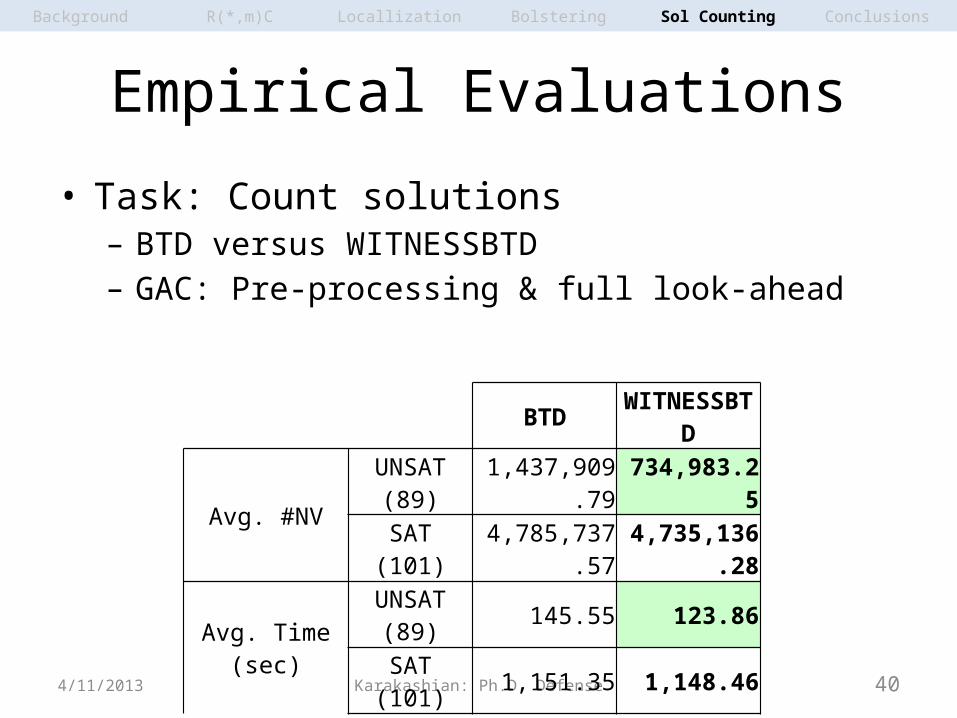
Empirical Evaluations
• Task: Count solutions – BTD versus WITNESSBTD – GAC: Pre-processing & full look-ahead
4/11/2013
Sol Counting Conclusions
BTD WITNESSBTD
Avg. #NVUNSAT (89) 1,437,909.79 734,983.25
SAT (101) 4,785,737.57 4,735,136.28
Avg. Time (sec)UNSAT (89) 145.55 123.86
SAT (101) 1,151.35 1,148.46
Background R(*,m)C Locallization Bolstering

Karakashian: Ph.D. Defense 41
Empirical Evaluations
4/11/2013
+ maxRPWC, m=2,4 wR( ,3)C∗ R( ,|∗ 𝜓(cli )|)C
#inst. GAC global local Proj. binary clique local Proj. binary clique
Completed
UNSAT479
20041.8%
19240.1%
24851.8%
23749.5%
23649.3%
22045.9%
30263.0%
29060.5%
28659.7%
27757.8%
SAT200
11155.5%
8542.5%
11256.0%
10050.0%
9648.0%
8140.5%
11055.0%
9045.0%
8844.0%
7839.0%
BT-Free
UNSAT479
00.0%
9720.3%
10421.7%
13929.0%
13929.0%
13127.3%
18638.8%
22146.1%
22246.3%
21244.3%
SAT200
157.5%
4221.0%
178.5%
4723.5%
4723.5%
4522.5%
2512.5%
6130.5%
6130.5%
5226.0%
Min(#NV
)
UNSAT479
20.4%
10121.1%
11123.2%
14530.3%
14530.3%
13628.4%
23549.1%
26354.9%
26455.1%
24450.9%
SAT200
199.5%
4221.0%
2311.5%
5226.0%
4924.5%
4924.5%
5728.5%
7437.0%
7336.5%
6532.5%
Fastest
UNSAT479
10020.9%
265.4%
12025.1%
7114.8%
234.8%
234.8%
18939.5%
12626.3%
5812.1%
5210.9%
SAT200
7336.5%
2010.0%
2010.0%
189.0%
94.5%
94.5%
2713.5%
157.5%
94.5%
94.5%
Sol Counting ConclusionsBackground R(*,m)C Locallization Bolstering
Karakashian: Ph.D. Defense 42
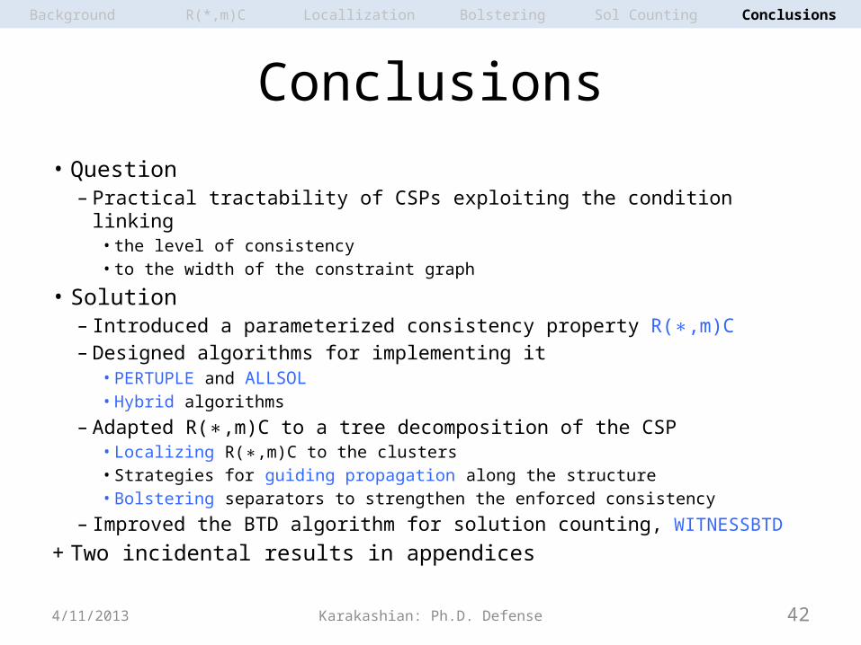
Conclusions• Question
– Practical tractability of CSPs exploiting the condition linking• the level of consistency • to the width of the constraint graph
• Solution– Introduced a parameterized consistency property R( ,m)C∗– Designed algorithms for implementing it
• PERTUPLE and ALLSOL• Hybrid algorithms
– Adapted R( ,m)C to a tree decomposition of the CSP∗• Localizing R( ,m)C to the clusters∗• Strategies for guiding propagation along the structure• Bolstering separators to strengthen the enforced consistency
– Improved the BTD algorithm for solution counting, WITNESSBTD
+ Two incidental results in appendices
4/11/2013
ConclusionsBackground R(*,m)C Locallization Bolstering Sol Counting

Karakashian: Ph.D. Defense 43
Future Research
• Extension to non-table constraints• Automating the selection of– a consistency property– consistency algorithms
[Geschwender+ 13]
• Characterizing performance on randomly generated problems
• + much more in dissertation
4/11/2013
ConclusionsBackground R(*,m)C Locallization Bolstering Sol Counting
Karakashian: Ph.D. Defense 444/11/2013
Thank You
Collaborations: Bessiere, Geschwender, Hartke, Reeson, Scott, Woodward.
Support: NSF CAREER Award #0133568 & NSF Grant No. RI-111795. Experiments were conducted on the equipment of the Holland Computing Center at UNL.

Karakashian: Ph.D. Defense 45
Computing All k-Connected Subgraphs
• Avoids enumerating non-connected k-subgraphs
• Competitive on large graphs with small k
4/11/2013
c d
eab
5 10 15 20 25 30 35 400
200400600800
1,0001,2001,4001,6001,800
Random: 500 vertices, k=4
ConSubg
LBF-ConSubg
BF-ConSubg
Degree
Tim
e (s
ec)
100 150 200 250 300 350 400 450 500 550 600 650 700 750 800 850 9000
500
1,000
1,500
2,000
2,500
3,000
3,500
Random: degree=40, k=4
ConSubg
LBF-ConSubg
BF-ConSubg
Number of Vertices
Tim
e (s
ec)

46
Solution Cover Problem is in NP-C
• Solution Cover Problem– Given a CSP with global constraints– is there a set of k solutions– such that ever tuple in the minimal CSP is covered by at
least one solution in the set? • Set Cover Problem Solution Cover Problem⟶• Set Cover Problem– Given a finite set U and a collection S of subsets of U– Are there k elements of S– Whose union is U?
4/11/2013 Karakashian: Ph.D. Defense


