Practical Radio Environment Mapping withGeostatistics

Caleb Phillips, Michael Ton, Douglas Sicker, and Dirk GrunwaldComputer Science Department

University of ColoradoBoulder, Colorado

Email: {caleb.phillips, michael.ton, sicker, grunwald}@colorado.edu

Abstract—In this paper we present results from the firstapplication of robust geostatistical modeling techniques to radioenvironment and coverage mapping of wireless networks. Weperform our analysis of these methods with a case study mappingthe coverage of a 2.5 GHz WiMax network at the University ofColorado, Boulder. Drawing from our experiences, we proposeseveral new methods and extensions to basic geostatistical theorythat are necessary for use in a radio mapping application. Wealso derive a set of best practices and discuss potential areas offuture work. We find that this approach to radio environmentmapping is feasible and produces maps that are more accurateand informative than both explicitly tuned path loss models andbasic data fitting approaches.

I. I NTRODUCTION

Today, wireless networks are ubiquitous and the importanceof their role in our daily lives cannot be underestimated. Toalarge extent, our ability to build and understand these networkshinges on understanding how wireless signals are attenuatedover distance in realistic environments. By predicting theattenuation of a radio signal we can better plan and diagnosenetworks as well as build futuristic networks that are awareof, and adapt to, the spatiotemporal radio environment. Forinstance, today’s network engineers need methods for accu-rately mapping the extent of coverage of existing and plannednetworks, yet the efficacy of those approaches is determinedby the predictive power of the underlying path loss model(or interpolation regime). Similarly, researchers that investigateDynamic Spectrum Access (DSA) networks require accurateRadio Environment Map (REM)s to automate appropriate andtimely frequency allocation decisions, yet the performanceof these systems is tied intimately to their ability to makemeaningful predictions about the current and future occupancyof the radio channel.

Although numerous models have been proposed to predictthe vagaries of the radio environmenta priori, in practice theerror associated with these models prevents their use in manyapplications [1]. The most promising of these models, whichinvolve explicit calculation of diffractions due to obstacles(e.g., [2]), may be more accurate, but have prohibitive datarequirements—precise vector models of all three dimensionalstructures (e.g., buildings and foliage). In the majority ofsituations where the available environmental data is limited orof low resolution, it is not clear how these models’ accuracyisaffected, and hence they may not be well enough understood

(a) (b)

Fig. 1. Examples of coverage map (for CU WiMax cuEN node) overlayedin Google Earth. Green regions indicate strong signal and red regions indicateweak signal.for practical use in applications that demand high fidelitymaps.

The limitations ofa priori models have led some researchersto an integrated solution that combines some number of carefulmeasurements with predictions (interpolation) (e.g., [3]). And,more recently, some researchers have looked to the promisingarea of geostatistics as a method of modeling the spatialstructure of the radio environment [4], [5]. In this paper,we give a first practical application of geostatistical methodsof spatial sampling and interpolation (termed “Kriging” inthe geostatistical literature) to the task of mapping the radioenvironment of a production wireless network. Our approachcomplimentsa priori modeling, by suggesting a statisticallyrobust method for using measurements tocorrect residualerror from deterministic models(e.g., ray-tracing or statisticalmethods) and common empirical fitting approaches to pre-dicting path loss (e.g., power law fitting). In this way, detailedmaps can be generated for both large scale fades, as well as aclear quantification of how small scale fades contribute to thespatial distribution of intrinsic channel variation. We carry outour evaluation using a 2.5 GHz WiMax network operated bythe University of Colorado at Boulder. We use our experiencesfrom this case study to develop a set of best-practices forthe geostatistical mapping of similar radio environments,andshow the real-world abilities of these methods. Figure 1 showsan example of a map produced by our method, overlayed onGoogle Earth.

In the next section, we will provide some background ongeostatistical modeling and on existing work that has proposed

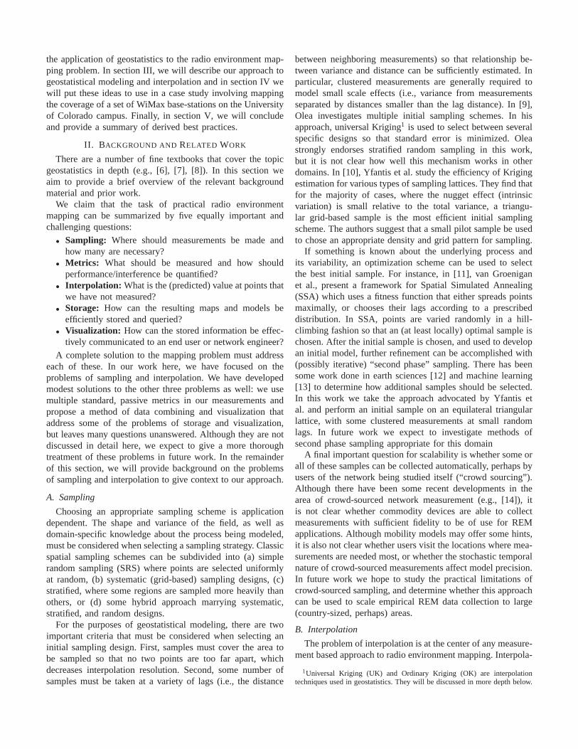
the application of geostatistics to the radio environment map-ping problem. In section III, we will describe our approach togeostatistical modeling and interpolation and in section IV wewill put these ideas to use in a case study involving mappingthe coverage of a set of WiMax base-stations on the Universityof Colorado campus. Finally, in section V, we will concludeand provide a summary of derived best practices.

II. BACKGROUND AND RELATED WORK

There are a number of fine textbooks that cover the topicgeostatistics in depth (e.g., [6], [7], [8]). In this section weaim to provide a brief overview of the relevant backgroundmaterial and prior work.

We claim that the task of practical radio environmentmapping can be summarized by five equally important andchallenging questions:

• Sampling: Where should measurements be made andhow many are necessary?

• Metrics: What should be measured and how shouldperformance/interference be quantified?

• Interpolation: What is the (predicted) value at points thatwe have not measured?

• Storage: How can the resulting maps and models beefficiently stored and queried?

• Visualization: How can the stored information be effec-tively communicated to an end user or network engineer?

A complete solution to the mapping problem must addresseach of these. In our work here, we have focused on theproblems of sampling and interpolation. We have developedmodest solutions to the other three problems as well: we usemultiple standard, passive metrics in our measurements andpropose a method of data combining and visualization thataddress some of the problems of storage and visualization,but leaves many questions unanswered. Although they are notdiscussed in detail here, we expect to give a more thoroughtreatment of these problems in future work. In the remainderof this section, we will provide background on the problemsof sampling and interpolation to give context to our approach.

A. Sampling

Choosing an appropriate sampling scheme is applicationdependent. The shape and variance of the field, as well asdomain-specific knowledge about the process being modeled,must be considered when selecting a sampling strategy. Classicspatial sampling schemes can be subdivided into (a) simplerandom sampling (SRS) where points are selected uniformlyat random, (b) systematic (grid-based) sampling designs, (c)stratified, where some regions are sampled more heavily thanothers, or (d) some hybrid approach marrying systematic,stratified, and random designs.

For the purposes of geostatistical modeling, there are twoimportant criteria that must be considered when selecting aninitial sampling design. First, samples must cover the areatobe sampled so that no two points are too far apart, whichdecreases interpolation resolution. Second, some number ofsamples must be taken at a variety of lags (i.e., the distance

between neighboring measurements) so that relationship be-tween variance and distance can be sufficiently estimated. Inparticular, clustered measurements are generally required tomodel small scale effects (i.e., variance from measurementsseparated by distances smaller than the lag distance). In [9],Olea investigates multiple initial sampling schemes. In hisapproach, universal Kriging1 is used to select between severalspecific designs so that standard error is minimized. Oleastrongly endorses stratified random sampling in this work,but it is not clear how well this mechanism works in otherdomains. In [10], Yfantis et al. study the efficiency of Krigingestimation for various types of sampling lattices. They findthatfor the majority of cases, where the nugget effect (intrinsicvariation) is small relative to the total variance, a triangu-lar grid-based sample is the most efficient initial samplingscheme. The authors suggest that a small pilot sample be usedto chose an appropriate density and grid pattern for sampling.

If something is known about the underlying process andits variability, an optimization scheme can be used to selectthe best initial sample. For instance, in [11], van Groeniganet al., present a framework for Spatial Simulated Annealing(SSA) which uses a fitness function that either spreads pointsmaximally, or chooses their lags according to a prescribeddistribution. In SSA, points are varied randomly in a hill-climbing fashion so that an (at least locally) optimal sample ischosen. After the initial sample is chosen, and used to developan initial model, further refinement can be accomplished with(possibly iterative) “second phase” sampling. There has beensome work done in earth sciences [12] and machine learning[13] to determine how additional samples should be selected.In this work we take the approach advocated by Yfantis etal. and perform an initial sample on an equilateral triangularlattice, with some clustered measurements at small randomlags. In future work we expect to investigate methods ofsecond phase sampling appropriate for this domain

A final important question for scalability is whether some orall of these samples can be collected automatically, perhaps byusers of the network being studied itself (“crowd sourcing”).Although there have been some recent developments in thearea of crowd-sourced network measurement (e.g., [14]), itis not clear whether commodity devices are able to collectmeasurements with sufficient fidelity to be of use for REMapplications. Although mobility models may offer some hints,it is also not clear whether users visit the locations where mea-surements are needed most, or whether the stochastic temporalnature of crowd-sourced measurements affect model precision.In future work we hope to study the practical limitations ofcrowd-sourced sampling, and determine whether this approachcan be used to scale empirical REM data collection to large(country-sized, perhaps) areas.

B. Interpolation

The problem of interpolation is at the center of any measure-ment based approach to radio environment mapping. Interpola-

1Universal Kriging (UK) and Ordinary Kriging (OK) are interpolationtechniques used in geostatistics. They will be discussed inmore depth below.

tion attempts to use some number of measurements to predictthe value at points that have not been measured. One solution,from the field of geostatistics, is known as Kriging after theseminal work of Dain Krige on mine valuation in the 1950’sand 60’s. As compared to alternative methods of interpolativemapping, such as Inverse Distance Weighting (IDW), Kriginghas three important benefits: (1) it is preceded by an analysisof the spatial structure of the data and an estimate of theaverage spatial variability of the data is integrated into theinterpolation process vis a vis the variogram model, (2) itis an exact interpolation method meaning that when data isavailable at a given point, the interpolated map has exactlythat measured value at that point, and (3) since it is a robuststatistical method, it provides a per-prediction indication ofestimation standard error via the square root of the Krigingvariance [7].

There have been several papers that have attempted to de-velop interpolation strategies appropriate for wireless coveragemapping. In [15], Connellyet al. suggest a way to interpolatebetween Received Signal Strength (RSS) measurements usingIDW and claim less than 1 dB interpolation error. Althoughpromising, this work makes strong simplifying assumptions(for instance, assuming propagation stops after 100 m), whichprohibit use in the applications we are considering here.In [16], Dall’Anese suggests a way to use distributed mea-surements from sensors to determine a sparsity promotingWeighted Least Squares (WLS) interpolated coverage map.The authors assume that the location of sensors is not con-trollable and that the principle application is in empiricallydetermining a safe transmit power for a given radio so asto avoid interfering with primary users (PUs). In [4], Konakproposes the use of Ordinary Kriging (OK) over grid-sampleddata for mapping coverage and shows that this approach canoutperform a neural network trained model presented in [17].Finally, [18] provides a tutorial addressing the use of basicgeostatistical interpolation for estimating radio-electric expo-sure levels. While not strictly the same as wireless networkpropagation, the approach is relevant.

In addition to these works, there have been several recentpublications by Riihijarvi et al. that discuss the use of spatialstatistics to model radio propagation [19], [5]. Like [4], thiswork presumes a sampling on a regular rectangular grid.Measurements are used to fit a semivariogram and severalunderlying functions are investigated. In [20], the authorssuggest how this method can be used to more compactly storeradio environment maps and in [21] the authors investigatehow the placement of transmitters, terrain roughness, andassumed path loss effects the efficacy of the interpolatedfield. In this paper, we build upon the foundational work ofRiihij arvi and Konak by making an empirical evaluation ofthese geostatistical techniques, applying them to the generalcase of coverage mapping, and evaluating them in a realisticenvironment.

III. M ETHOD

If we assume that there is a random field that we aremodeling calledZ, then the value of that field at a point inspacex is Z(x). The field can be defined in any dimension,but typically we would assume thatx ∈ R

n with n = 2 orn = 3. We can then define the value at any point as the fieldmean (µ) plus some error (ǫ(x)):

Z(x) = µ+ ǫ(x) (1)

This model, which is used in Ordinary Kriging (OK),assumes a constant (stationary) mean in space. Generalizationsthat drop this assumption allow for nonlinear constructions andare generally termed Universal Kriging (UK), but are likelyoverpowered for this application. As we will show below, OKmethods are sufficiently powerful if care is taken to removetrend (bias) from the process prior to modeling.

A. The Variogram

Central to geostatistics is the variogram, a function thatmodels the variance between two points in space as a functionof the distance between them (h). In the case of grid-sampledfields, the distance between measurements is a fixed lag dis-tance. Randomized and optimized sampling schemes producevariable lag distances. The theoretical variogram is typicallywritten as:

γ(h) =1

2E[(Z(x+ h)− Z(x))2] (2)

If we know that the field is second order stationary (i.e., ameasurement at the same point will not vary with time, andthedifferencebetween two measurements is also constant withtime), then the covariance function (correllelogram) is definedas:

C(h) = E[(Z(x)− µ)(Z(x+ h)− µ)] = C(0)− γ(h) (3)

The assumption of second order stationarity may not besafe for many radio environments, especially those operatingat low frequencies. Extending our work here to incorporatenonstationary models is an exciting area for future work thatis outside of the scope at present.

If we have some set of measurements, we can define anempirical variogram:

γ′(hi) =1

2n

n∑

j=1

(Z(xj + hi)− Z(xj))2 (4)

A typical problem is to fit a variogram model (or correllel-ogram) to an empirical variogram curve, given some numberof measurements. There are a number of models that can beused for fitting. One example is the exponential model:

γexp(h) = τ2 + σ2(1− e−h/φ) (5)

In this equation,τ2 is known as the nugget variance andis used to model discontinuity around the origin. In radio,

this would correspond to the intrinsic variation (small scalefading) of the channel.σ2 is known as the sill because it setsthe maximum value (variance) of the semivariogram. Largervalues ofσ will increase the level at which the curve flattensout. Finally, the parameterφ acts as a scale and affects theoverall shape of the curve. The value ofφ determines therate at which variance is expected to appear as a function ofdistance (lag) between points. There are a number of othermodels, such as the Gaussian, Cauchy, and Matern models,which may or may not be the best fit depending on the data2.As we will see for the networks and metrics we study here,the classical Gaussian and Cubic models perform well. Inthis work we perform variogram fitting using the weightedleast squares (WLS) method described in [23], using theimplementation available in the R package “geoR” [24]. Inour implementation, variogram fitting is automated by fittingmultiple functions and parameter combinations and choosingthe best fit via cross validation. Although computationallyintense, this fitting process can be trivially parallelizedso thatit can be accomplished quickly. For instance, by computingand cross-validating fits in parallel. Data-parallelism can alsobe acheived by fitting measurements from each transmitterseparately, in parallel.

B. Kriging

OK is an interpolation technique that predicts the unknownvalue at a new location (Z(x′)) from the weighted knownvalues at neighboring locations (xi):

ZK(x′) =

n∑

i=0

wiZ(xi) (6)

To determine the optimal weights (w), we must minimize theestimation varianceσ2

E :

σ2

E = E[(Zk(x′)− Z(x′)2] (7)

where

σ2

E = −γ(x′−x′)−

n∑

i=1

n∑

j=1

wiwjγ(xi−xj)+2

n∑

i=1

wiγ(xi−x′)

(8)which leads to the system of equations:

γ(x1 − x1) · · · γ(x1 − xn) 1...

. . ....

...γ(xn − x1) · · · γ(xn − xn) 1

1 . . . 1 0

w1

...wn

µ

(9)

=

γ(x1 − x0)...

γ(xn − x0)1

2[22] provides an excellent survey of these models.

whereµ is called the Lagrange parameter. This interpolationis “exact”, meaning thatZK(x′) = Z(x) if x = x

′. Thisapproach can be used for mapping by Kriging the value ateach pixel position. In this application, the system in equation9 is solved for each unknown pixel value (x

′). This constitutesa substantial amount of work, but is trivially parallelizeable(e.g., by performing each pixel calculation simultaneously).

The quality of an interpolated field depends on the goodnessof the fitted variogram (γ). In addition to this, there area number of different ways to adapt Kriging to a specificdata set. Anisotropic corrections are of particular interestfor coverage mapping. This approach assumes that the fieldmay require different statistics (i.e., a different variogram andpossibly fitting method) in different directions from somepoint. There is also an entire branch of statistics dealing withmultivariate analysis (co-Kriging).

C. Detrending

In [22], Olea et al describe the importance of removingany sources of nonlinear trend from measurements so thatthe fitted (interpolated) field complies with the basic tenetsof geostatistics. To this end, we introduce a hybrid approachwhere a predictive (empirical) model is used to calculate thepredicted path loss value at each measurement point. Thisapproach differs from the direct fitting method suggested byRiihij arvi and Konak. In our method, the model prediction issubtracted from the observed value to obtain the residual, orerror:

Z ′(x) = Z(x)− P (x) (10)

whereZ ′() is the residual (de-trended measurements) process,Z() is the observed process andP () is the model predic-tion. This approach to detrending is entirely modular andextensible—P () can be replaced with any predictive model.In this way, the geostatistical interpolation can be viewedas a careful way to correct for any remaining (environmentspecific) model error, instead of as a complete replacement.And, as the state of the art in path loss modeling is advancedfurther, and models are able to make predictions closer tomeasurements, this improvement can be carried through tomeasurement-based interpolation in the process of de-trendingas described here.

In our work here, we detrend signal strength measurementswith a fitted model for path loss from [1]. First, we convertthe measurements from signal power/ratio (i.e., Carrier toInterference and Noise Ratio (CINR)), to path loss. Thisrequires some basic knowledge about the transmitter: transmitpower (Ptx in dBm), antenna gain in the direction of thereceiver (Gtx(θ) in dB), and an assumed constant noise floorvalue (N in dBm, set to -95 here).

Zpl(x) = (Ptx +Gtx(θ))−N − Zcinr(x) (11)

If this information is not known, approximate values canbe substituted which will be corrected automatically in the

fitting process, and should have no discernable ill-effect onthe accuracy of the interpolation.

Using the observations from each transmitter, we fit the pa-rametersα (path loss exponent) andǫ (offset) in the followingequation:

P (x) = α10log10(d) + 20log10(f) + 32.45 + ǫ (12)

where d is the distance from the pointx to the transmitterin km and f is the frequency of the transmission in MHz.Subtracting the fitted value ofP () for from each measurementgives the de-trended observations (Z ′(x)), which can then beused to fit an empirical variogram model.

D. Summary of Complete Method

In summary, the complete mapping process is as follows:We begin by determining the extent of the area of interest,and defining a bounding box for measurements (and predic-tion). Following the best practices for geostatistical samplingdescribed in section II-A, a uniform (equilateral triangular)sample grid is generated and used for the initial sampling.Some small number of pilot measurements may be necessaryto determine an appropriate lag distance (sampling density)for this grid.

Next, measurements are taken at the grid points. At a subsetof grid locations, random clustered measurements are alsotaken within 40 wavelengths (4.8 m) of the original point.When the resulting data from the initial sample is available,it must be inspected for sources of systematic bias andmeasurement error. Sources of measurement error may differfrom campaign to campaign, but are generally systematic (i.e.,equipment or procedural error) or spatial (i.e., sources oferroror interference stemming from the position of the measurementapparatus relative to its surroundings). When bias is suspectedin the measurements, these issues must be approached on acase-by-case basis.

Next, using the method described in section III-C, wedetrend the measurements. The detrended measurements arethen used to generate an empirical variogram, and theoreticalvariogram fit as described in section III-A. Using the vari-ogram and measurements, a WLS OK method can be used tointerpolate the values at each pixel location. We recommend0.2 pixels per meter for high resolution maps, and 0.05 pixelsper meter for low resolution (prototyping) maps.

The OK process produces a map with an interpolatedvalue and error (Kriging variance) at each pixel location.This step requires substantial computation (especially athighresolutions). Optionally, second-phase samples can be takento fine tune the model and reduce residual error further. Aftereach round of additional sampling, the variogram fitting andKriging steps must be repeated. Finally, the trend is addedback to pixel values to produce a final raster image.

IV. CASE STUDY: WIMAX

In this section, we describe a case study conducted specif-ically for the purpose of evaluating the efficacy of Kriging-based coverage mapping. Our aim here is to map the coverage

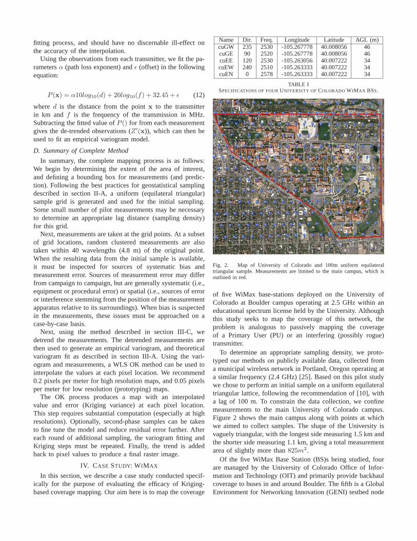
Name Dir. Freq. Longitude Latitude AGL (m)cuGW 235 2530 -105.267778 40.008056 46cuGE 90 2520 -105.267778 40.008056 46cuEE 120 2530 -105.263056 40.007222 34cuEW 240 2510 -105.263333 40.007222 34cuEN 0 2578 -105.263333 40.007222 34

TABLE ISPECIFICATIONS OF FOURUNIVERSITY OF COLORADO WIMAX BSS.

Fig. 2. Map of University of Colorado and 100m uniform equilateraltriangular sample. Measurements are limited to the main campus, which isoutlined in red.

of five WiMax base-stations deployed on the University ofColorado at Boulder campus operating at 2.5 GHz within aneducational spectrum license held by the University. Althoughthis study seeks to map the coverage of this network, theproblem is analogous to passively mapping the coverageof a Primary User (PU) or an interfering (possibly rogue)transmitter.

To determine an appropriate sampling density, we proto-typed our methods on publicly available data, collected froma municipal wireless network in Portland, Oregon operatingata similar frequency (2.4 GHz) [25]. Based on this pilot studywe chose to perform an initial sample on a uniform equilateraltriangular lattice, following the recommendation of [10],witha lag of 100 m. To constrain the data collection, we confinemeasurements to the main University of Colorado campus.Figure 2 shows the main campus along with points at whichwe aimed to collect samples. The shape of the University isvaguely triangular, with the longest side measuring 1.5 km andthe shorter side measuring 1.1 km, giving a total measurementarea of slightly more than825m2.

Of the five WiMax Base Station (BS)s being studied, fourare managed by the University of Colorado Office of Infor-mation and Technology (OIT) and primarily provide backhaulcoverage to buses in and around Boulder. The fifth is a GlobalEnvironment for Networking Innovation (GENI) testbed node

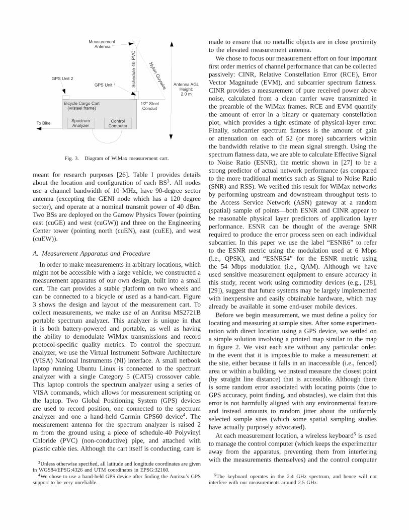
Fig. 3. Diagram of WiMax measurement cart.

meant for research purposes [26]. Table I provides detailsabout the location and configuration of each BS3. All nodesuse a channel bandwidth of 10 MHz, have 90-degree sectorantenna (excepting the GENI node which has a 120 degreesector), and operate at a nominal transmit power of 40 dBm.Two BSs are deployed on the Gamow Physics Tower (pointingeast (cuGE) and west (cuGW)) and three on the EngineeringCenter tower (pointing north (cuEN), east (cuEE), and west(cuEW)).

A. Measurement Apparatus and Procedure

In order to make measurements in arbitrary locations, whichmight not be accessible with a large vehicle, we constructedameasurement apparatus of our own design, built into a smallcart. The cart provides a stable platform on two wheels andcan be connected to a bicycle or used as a hand-cart. Figure3 shows the design and layout of the measurement cart. Tocollect measurements, we make use of an Anritsu MS2721Bportable spectrum analyzer. This analyzer is unique in thatit is both battery-powered and portable, as well as havingthe ability to demodulate WiMax transmissions and recordprotocol-specific quality metrics. To control the spectrumanalyzer, we use the Virtual Instrument Software Architecture(VISA) National Instruments (NI) interface. A small netbooklaptop running Ubuntu Linux is connected to the spectrumanalyzer with a single Category 5 (CAT5) crossover cable.This laptop controls the spectrum analyzer using a series ofVISA commands, which allows for measurement scripting onthe laptop. Two Global Positioning System (GPS) devicesare used to record position, one connected to the spectrumanalyzer and one a hand-held Garmin GPS60 device4. Themeasurement antenna for the spectrum analyzer is raised 2m from the ground using a piece of schedule-40 PolyvinylChloride (PVC) (non-conductive) pipe, and attached withplastic cable ties. Although the cart itself is conducting,care is

3Unless otherwise specified, all latitude and longitude coordinates are givenin WGS84/EPSG:4326 and UTM coordinates in EPSG:32160.

4We chose to use a hand-held GPS device after finding the Anritsu’s GPSsupport to be very unreliable.

made to ensure that no metallic objects are in close proximityto the elevated measurement antenna.

We chose to focus our measurement effort on four importantfirst order metrics of channel performance that can be collectedpassively: CINR, Relative Constellation Error (RCE), ErrorVector Magnitude (EVM), and subcarrier spectrum flatness.CINR provides a measurement of pure received power abovenoise, calculated from a clean carrier wave transmitted inthe preamble of the WiMax frames. RCE and EVM quantifythe amount of error in a binary or quaternary constellationplot, which provides a tight estimate of physical-layer error.Finally, subcarrier spectrum flatness is the amount of gainor attenuation on each of 52 (or more) subcarriers withinthe bandwidth relative to the mean signal strength. Using thespectrum flatness data, we are able to calculate Effective Signalto Noise Ratio (ESNR), the metric shown in [27] to be astrong predictor of actual network performance (as comparedto the more traditional metrics such as Signal to Noise Ratio(SNR) and RSS). We verified this result for WiMax networksby performing upstream and downstream throughput tests tothe Access Service Network (ASN) gateway at a random(spatial) sample of points—both ESNR and CINR appear tobe reasonable physical layer predictors of application layerperformance. ESNR can be thought of the average SNRrequired to produce the error process seen on each individualsubcarrier. In this paper we use the label “ESNR6” to referto the ESNR metric using the modulation used at 6 Mbps(i.e., QPSK), and “ESNR54” for the ESNR metric usingthe 54 Mbps modulation (i.e., QAM). Although we haveused sensitive measurement equipment to ensure accuracy inthis study, recent work using commodity devices (e.g., [28],[29]), suggest that future systems may be largely implementedwith inexpensive and easily obtainable hardware, which mayalready be available in some end-user mobile devices.

Before we begin measurement, we must define a policy forlocating and measuring at sample sites. After some experimen-tation with direct location using a GPS device, we settled ona simple solution involving a printed map similar to the mapin figure 2. We visit each site without any particular order.In the event that it is impossible to make a measurement atthe site, either because it falls in an inaccessible (i.e., fenced)area or within a building, we instead measure the closest point(by straight line distance) that is accessible. Although thereis some random error associated with locating points (due toGPS accuracy, point finding, and obstacles), we claim that thiserror is not harmfully aligned with any environmental featureand instead amounts to random jitter about the uniformlyselected sample sites (which some spatial sampling studieshave actually purposely advocated).

At each measurement location, a wireless keyboard5 is usedto manage the control computer (which keeps the experimenteraway from the apparatus, preventing them from interferingwith the measurements themselves) and the control computer

5The keyboard operates in the 2.4 GHz spectrum, and hence will notinterfere with our measurements around 2.5 GHz.

provides feedback through an amplified speaker utilizing text-to-speech synthesis software. At each point, three repeatedmeasurements are made of downstream system performanceusing the various metrics. At a subset of points, additionalclustered measurements were taken within a 40 wavelength(≈ 4.8 m) radius of each true point. The combination ofrepeating measurements in time and space, allows for accurateestimation and averaging of intrinsic channel variabilitydueto small scale fading effects and instrument error.

The device first picks a given channel (carrier frequency)and then records all metrics for each measurement in turn.Then it switches to a different channel and repeats. While thedevice is performing measurements, the experimenter uses thehandheld GPS device to record the current position, samplelocation (each sample site is assigned a unique identifier),andGPS accuracy. At the end of a measurement effort (typicallywhen the analyzer’s battery is flat), the cart is returned tothe laboratory for charging and data offload. The spectrumanalyzer stores measurements in a proprietary, but plain/text,format that can be easily parsed.

B. Possible Sources of Systematic Sampling Error

During our measurement campaign, three individuals usedthe cart to make measurements. Although all three measurerswere collecting measurements using the same procedure, onepossible source of systematic error is from the measurersthemselves. No significant correlation is present in terms oflocation error or measurement variation and hence we donot correct for this bias in subsequent analysis. It is worthnoting that some measurements are distant from their intendedlocation. This occurs (as discussed above), when a point isunreachable. So long as the new measurement point is asclose to the original measurement location as possible andthere is no systematic error or systematic terrain alignment,these deviations should not effect the quality of the sample.We also investigated the relationship between GPS accuracyand channel variation, hypothesizing that GPS accuracy mightbe weaker in complex environments where signal is alsodegraded, but no discernible correlation was present.

C. Correlation Between Metrics

In this measurement campaign, we collected several per-formance metrics besides the classic signal strength or SNR-equivalent metrics. One question that naturally arises is:arethese more robust metrics trivially correlated with simpleand easy to collect metrics such as CINR. Figure 4 plotsthe relationship between CINR and each of the other met-rics studied. RCE and EVM appear to be a simple (butnonlinear) function of CINR, at least as calculated by thespectrum analyzer used in this study. There are several waysthat EVM can be calculated from the constellation plot andobserved power of constellation points. It appears that theAnritsu spectrum analyzer is calculating EVM from CINR orvice versa. RCE is calculated directly from the EVM valueand hence is equivalent. Given this, RCE and EVM do notappear to provide novel information above and beyond what

CINR versus RMS RCE

RMS RCE

CIN

R

10

20

30

40

−30 −20 −10 0

(a) RCE

CINR versus RMS EVM

RMS EVM

CIN

R

10

20

30

40

0 20 40 60 80 100

(b) EVM

Effective SNR (6) versus CINR

ESNR6

CIN

R

10

20

30

40

10 20 30 40

(c) ESNR6

Effective SNR (54) versus CINR

ESNR54

CIN

R

10

20

30

40

15 20 25 30 35 40 45

(d) ESNR54

Fig. 4. Correlation between metrics and CINR.

is provided by the CINR measurement. It is worth notingthat in the process of data collection, we have recorded acomplete constellation plot for each measurement so we couldalso calculate RCE ourselves. The relationship between ESNRand CINR is less trivial, especially for the lower (Phase ShiftKeying (PSK) modulation based) bitrates. The higher bitrates,which use Quadrature Amplitude Modulation (QAM), tendto have a fairly well defined linear correlation with CINR.A least squares fit of ESNR54 to CINR is very good withadjustedR2 of 0.90 and mean residual error of 1.01 (ascompared with 0.29R2 and 8 dB residual error for ESNR6).This suggests that in cases where information about spectrumflatness is unavailable, ESNR54 can be roughly approximatedusing CINR measurements.

D. Spatial Data Characterization and Variogram Fitting

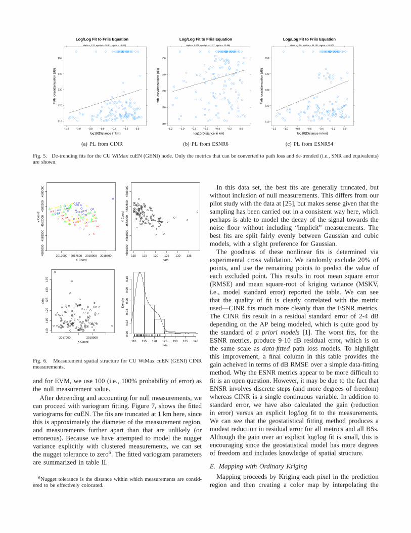
Figure 6 shows CINR measurements taken for the “cuEN”BS. By plotting the measurements in this way, we can identifyany sources of skew and bias in the measurements, as wellas understand their distributional spread and variance priorto geostatistical modeling. All four metrics produce a similarspatial distribution of values with large path loss or errorvalues to the southwest and smaller (better) values to thenorth. All metrics have different value distributions, buttheESNR54 and and CINR metrics appear to share the same basicskewed lognormal shape. Figure 5 shows the fitted relationshipbetween path loss and distance for the three SNR-like metrics.The fits are poor, but appear to at least account for some basictrend, which we can remove to improve the efficacy of theKriging process. At locations where we attempt, but fail, tomake a measurement, we use a noise-floor value. We call these“null measurements”. For the SNR-like metrics, we use 1.0

Log/Log Fit to Friis Equation

log10(Distance in km)

Pat

h lo

ss/a

ttenu

atio

n (d

B)

110

120

130

140

150

−1.2 −1.0 −0.8 −0.6 −0.4 −0.2 0.0

alpha = 1.22, epsilon = 28.81, sigma = 16.802

(a) PL from CINR

Log/Log Fit to Friis Equation

log10(Distance in km)

Pat

h lo

ss/a

ttenu

atio

n (d

B)

110

120

130

140

150

−1.2 −1.0 −0.8 −0.6 −0.4 −0.2 0.0

alpha = 1.071, epsilon = 41.37, sigma = 13.884

(b) PL from ESNR6

Log/Log Fit to Friis Equation

log10(Distance in km)

Pat

h lo

ss/a

ttenu

atio

n (d

B)

110

120

130

140

150

−1.2 −1.0 −0.8 −0.6 −0.4 −0.2 0.0

alpha = 1.56, epsilon = 34.151, sigma = 16.972

(c) PL from ESNR54

Fig. 5. De-trending fits for the CU WiMax cuEN (GENI) node. Only the metrics that can be converted to path loss and de-trended(i.e., SNR and equivalents)are shown.

2017000 2017500 2018000 20185004581

000

4581

500

4582

000

4582

500

4583

000

X Coord

Y C

oord

110 115 120 125 130 1354581

000

4581

500

4582

000

4582

500

4583

000

data

Y C

oord

2017000 2018000

110

115

120

125

130

135

X Coord

data

data

Den

sity

110 115 120 125 130 135 140

0.00

0.02

0.04

0.06

0.08

0.10

Fig. 6. Measurement spatial structure for CU WiMax cuEN (GENI) CINRmeasurements.

and for EVM, we use 100 (i.e., 100% probability of error) asthe null measurement value.

After detrending and accounting for null measurements, wecan proceed with variogram fitting. Figure 7, shows the fittedvariograms for cuEN. The fits are truncated at 1 km here, sincethis is approximately the diameter of the measurement region,and measurements further apart than that are unlikely (orerroneous). Because we have attempted to model the nuggetvariance explicitly with clustered measurements, we can setthe nugget tolerance to zero6. The fitted variogram parametersare summarized in table II.

6Nugget tolerance is the distance within which measurements are consid-ered to be effectively colocated.

In this data set, the best fits are generally truncated, butwithout inclusion of null measurements. This differs from ourpilot study with the data at [25], but makes sense given that thesampling has been carried out in a consistent way here, whichperhaps is able to model the decay of the signal towards thenoise floor without including “implicit” measurements. Thebest fits are split fairly evenly between Gaussian and cubicmodels, with a slight preference for Gaussian.

The goodness of these nonlinear fits is determined viaexperimental cross validation. We randomly exclude 20% ofpoints, and use the remaining points to predict the value ofeach excluded point. This results in root mean square error(RMSE) and mean square-root of kriging variance (MSKV,i.e., model standard error) reported the table. We can seethat the quality of fit is clearly correlated with the metricused—CINR fits much more cleanly than the ESNR metrics.The CINR fits result in a residual standard error of 2-4 dBdepending on the AP being modeled, which is quite good bythe standard ofa priori models [1]. The worst fits, for theESNR metrics, produce 9-10 dB residual error, which is onthe same scale asdata-fittedpath loss models. To highlightthis improvement, a final column in this table provides thegain acheived in terms of dB RMSE over a simple data-fittingmethod. Why the ESNR metrics appear to be more difficult tofit is an open question. However, it may be due to the fact thatENSR involves discrete steps (and more degrees of freedom)whereas CINR is a single continuous variable. In addition tostandard error, we have also calculated the gain (reductionin error) versus an explicit log/log fit to the measurements.We can see that the geostatistical fitting method produces amodest reduction in residual error for all metrics and all BSs.Although the gain over an explicit log/log fit is small, this isencouraging since the geostatistical model has more degreesof freedom and includes knowledge of spatial structure.

E. Mapping with Ordinary Kriging

Mapping proceeds by Kriging each pixel in the predictionregion and then creating a color map by interpolating the

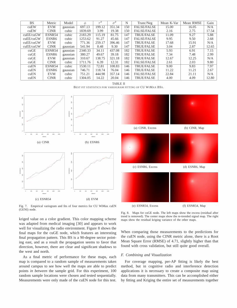
BS Metric Model φ τ2 σ2 N Trunc/Neg Mean K-Var Mean RMSE GaincuEW EVM gaussian 697.13 199.12 351.34 150 FALSE/FALSE 15.00 16.05 N/AcuEW CINR cubic 1839.69 3.99 19.38 150 FALSE/FALSE 2.16 2.75 17.54

cuEE/cuGW ESNR54 cubic 2183.29 115.19 81.75 147 TRUE/FALSE 11.09 9.27 5.88cuEE/cuGW ESNR6 cubic 1253.62 91.27 45.66 147 FALSE/FALSE 9.95 9.50 2.68cuEE/cuGW EVM cubic 771.36 259.17 396.46 147 TRUE/FALSE 17.68 15.91 N/AcuEE/cuGW CINR gaussian 541.94 8.48 9.30 147 TRUE/FALSE 3.04 2.87 12.65

cuGE ESNR54 gaussian 2340.33 34.11 437.08 182 TRUE/FALSE 5.93 6.91 7.15cuGE ESNR6 gaussian 380.27 49.67 39.18 182 TRUE/FALSE 7.34 7.48 2.99cuGE EVM gaussian 310.67 138.75 321.18 182 TRUE/FALSE 12.67 12.25 N/AcuGE CINR cubic 1711.76 6.39 12.31 182 FALSE/FALSE 2.61 2.03 9.80cuEN ESNR54 cubic 1530.11 72.81 108.83 146 TRUE/FALSE 9.00 9.83 7.97cuEN ESNR6 gaussian 746.71 118.74 76.04 146 TRUE/FALSE 11.22 11.21 2.67cuEN EVM cubic 751.21 444.98 357.14 146 FALSE/FALSE 22.84 21.11 N/AcuEN CINR cubic 1304.05 14.22 20.04 146 TRUE/FALSE 4.00 4.09 12.80

TABLE IIBEST FIT STATISTICS FOR VARIOGRAM FITTING OFCU WIMAX BSS.

0 200 400 600 800 1000 1200

010

020

030

040

050

0

distance

sem

ivar

ianc

e

(a) CINR

0 200 400 600 800 1000 1200

050

100

150

200

250

300

distance

sem

ivar

ianc

e

(b) ESNR6

0 200 400 600 800 1000 1200

010

020

030

040

050

0

distance

sem

ivar

ianc

e

(c) ESNR54

0 200 400 600 800 1000 1200

050

010

0015

0020

00

distance

sem

ivar

ianc

e

(d) EVM

Fig. 7. Empirical variogram and fits of four metrics for CU WiMaxcuEN(GENI) node.

kriged value on a color gradient. This color mapping schemewas adapted from medical imaging [30] and appears to workwell for visualizing the radio environment. Figure 8 shows thefinal maps for the cuGE node, which features an interestingfinal propagation pattern. This BS is a 90-degree sector point-ing east, and as a result the propagation seems to favor thatdirection, however, there are clear and significant shadowstothe west and north.

As a final metric of performance for these maps, eachmap is compared to a random sample of measurements takenaround campus to see how well the maps are able to predictpoints in betweenthe sample grid. For this experiment, 100random sample locations were chosen and tested sequentially.Measurements were only made of the cuEN node for this test.

(a) CINR, Excess (b) CINR, Map

(c) ESNR6, Excess (d) ESNR6, Map

(e) ESNR54, Excess (f) ESNR54, Map

Fig. 8. Maps for cuGE node. The left maps show the excess (residual aftertrend is removed). The center maps show the re-trended signal map. The rightmaps show the residual kriging variance of the other maps.

When comparing those measurements to the predictions forthe cuEN node, using the CINR metric alone, there is a RootMean Square Error (RMSE) of 4.71, slightly higher than thatfound with cross validation, but still quite good overall.

F. Combining and Visualization

For coverage mapping, per-AP fitting is likely the bestmethod, but in cognitive radio and interference detectionapplications it is necessary to create a composite map usingdata from many transmitters. This can be accomplished eitherby fitting and Kriging the entire set of measurements together

or by fitting and Kriging measurements from each transmit-ter separately and then combining the resulting maps. Thefirst approach is the most conceptually straight forward, buthas some problems. Combining measurements from multipletransmitters may produce a map with a large amount of per-location variation, possibly with colocated points of drasticallyvarying value. Exactly colocated measurements of differingvalue can produce unsolvable Kriging equations and must be“jittered” to create a solvable equation with a unique solution.In the end, this approach can result in a map that is difficultto interpret and has a large error margin.

Due to the large variance at the same point due to differenttransmitters, the resulting map takes the form of a nearlyconstant value with peaks or holes centered at measurementlocations. As a result, these data-combined maps do notprovide information about the predicted coverage betweenpoints and are generally no more useful than simple color-coded dots located on a map. Given these concerns aboutthis data combining method, we advocate anex post factocombining which we will describe next.

Ex post factomap combining involves basic geospatialimage tiling and combination. We use a basic two-pass methodthat first reads in all the map files to determine the totalextent of the image, and then overlays the images, combiningvalues at pixels as necessary. There are many ways we cancombine maps this way, the most obvious is to take themaximum value for SNR-like metrics or the minimum valuefor EVM-like metrics. Figure 9 provides the combined mapsfor the CU WiMax measurements using these two combiningmethods. In the threshold-based combining, we count thenumber of transmitters whose interpolated signal is above 40dB CINR7(or below 60% in the case of the EVM metrics) anduse this count (from 0 to 4) for the map. For the maximum-based combining, we actually use the minimum for the EVMmetric, since a small value is good in this case. In a cognitiveradio application, a threshold-based map like this could beused to locate contiguous regions where it is safe to transmit.

These maps make light of a few interesting observations.Firstly, the threshold maps make it plain to see regions and thecontours between them where there is no coverage above thegiven threshold (light red) or substantial overlap (light green).Since two transmitters actually share the same frequency inthis network, regions of light green might actually indicatepotential for interference at the receiver. The maximum com-bining approach is less easy to interpret, but gives a completepicture of the propagation environment on the CU campus. Forall metrics, there appears to be a coverage “hole” just west ofthe Gamow tower, located in the center of the map, which mayindicate a misconfiguration in the downtilt of the west-pointingantennas for a building of this height (i.e., more downtilt mightbe necessary to avoid this hole). Additionally, the west-facingtransmitters on the other tower, may fail to cover this regionsince the Gamow tower creates a shadow. Despite the seeming

7This threshold was empirically derived using a random (spatial) sampleof upstream and downstream throughput measurements.

(a) CINR, Map (b) CINR

(c) ESNR6, Map (d) ESNR6

(e) ESNR54, Map (f) ESNR54

Fig. 9. Kriged maps for combined CU WiMax measurements using theCINR metric.

congruity of the maximum combined maps, the threshold mapsreveal fairly disparate contours.

G. Small Scale Effects and Nonstationarity

In this section we want to understand how measurementsvary over small time scales and small distances. An under-lying assumption of the Kriging process is that the processbeing modeled is stationary, meaning that the (fitted)meanisconstant in both time and space. Clearly, this is a strong as-sumption that the (often chaotic) radio environment is unlikelyto obey. It is possible to loosen the stationarity assumptionat the cost of substantial additional computational work, butin practice most users of Kriging processes opt to acceptthe implications of this assumption. By understanding howthe radio environment changes over small time scales andsmall distances, we can put a bound on repeated measurementvariation and hence a bound on the implicit unavoidable errorassociated with the stationarity assumption.

Fading in the radio environment can be classified intosmall-scale and large-scale fades. Large scale fades shouldbe fairly constant over small distances and time, and henceare not troublesome—it is exactly the environment-specificlarge scale fading effects that our approach models. However,small-scale fades can be highly varying in time and oversmall distances because they stem from multipath effects and(possibly mobile) scatterers. As a practical rule of thumb manyexperimenters average measurements within 40 wavelengths(≈ 4.8 m) as a way to “average out” small scale effects [31].In this section we seek to validate that standard practice aswell as understand the scale of small scale effects over short

CINR Spread (Range)

Den

sity

0.00

0.05

0.10

0.15

0.20

−5 0 5 10 15 20 25

FALSE

−5 0 5 10 15 20 25

TRUE

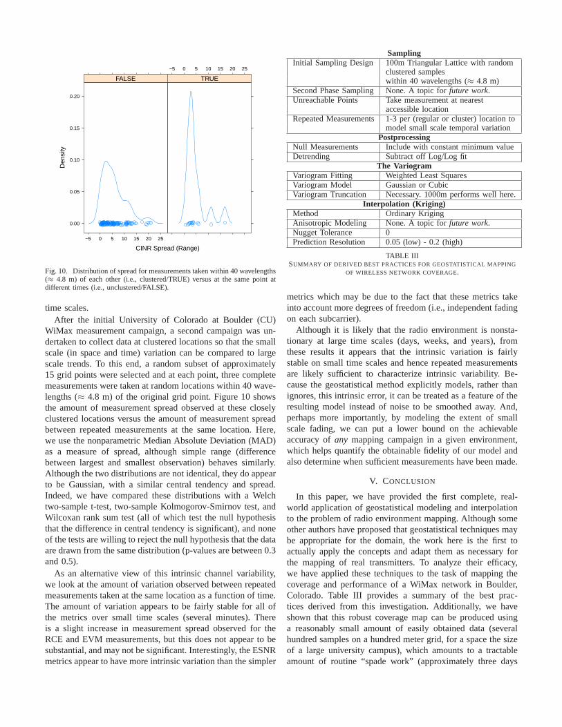
Fig. 10. Distribution of spread for measurements taken within40 wavelengths(≈ 4.8 m) of each other (i.e., clustered/TRUE) versus at the same point atdifferent times (i.e., unclustered/FALSE).

time scales.After the initial University of Colorado at Boulder (CU)

WiMax measurement campaign, a second campaign was un-dertaken to collect data at clustered locations so that the smallscale (in space and time) variation can be compared to largescale trends. To this end, a random subset of approximately15 grid points were selected and at each point, three completemeasurements were taken at random locations within 40 wave-lengths (≈ 4.8 m) of the original grid point. Figure 10 showsthe amount of measurement spread observed at these closelyclustered locations versus the amount of measurement spreadbetween repeated measurements at the same location. Here,we use the nonparametric Median Absolute Deviation (MAD)as a measure of spread, although simple range (differencebetween largest and smallest observation) behaves similarly.Although the two distributions are not identical, they do appearto be Gaussian, with a similar central tendency and spread.Indeed, we have compared these distributions with a Welchtwo-sample t-test, two-sample Kolmogorov-Smirnov test, andWilcoxan rank sum test (all of which test the null hypothesisthat the difference in central tendency is significant), andnoneof the tests are willing to reject the null hypothesis that the dataare drawn from the same distribution (p-values are between 0.3and 0.5).

As an alternative view of this intrinsic channel variability,we look at the amount of variation observed between repeatedmeasurements taken at the same location as a function of time.The amount of variation appears to be fairly stable for all ofthe metrics over small time scales (several minutes). Thereis a slight increase in measurement spread observed for theRCE and EVM measurements, but this does not appear to besubstantial, and may not be significant. Interestingly, theESNRmetrics appear to have more intrinsic variation than the simpler

SamplingInitial Sampling Design 100m Triangular Lattice with random

clustered sampleswithin 40 wavelengths (≈ 4.8 m)

Second Phase Sampling None. A topic forfuture work.Unreachable Points Take measurement at nearest

accessible locationRepeated Measurements1-3 per (regular or cluster) location to

model small scale temporal variationPostprocessing

Null Measurements Include with constant minimum valueDetrending Subtract off Log/Log fit

The VariogramVariogram Fitting Weighted Least SquaresVariogram Model Gaussian or CubicVariogram Truncation Necessary. 1000m performs well here.

Interpolation (Kriging)Method Ordinary KrigingAnisotropic Modeling None. A topic forfuture work.Nugget Tolerance 0Prediction Resolution 0.05 (low) - 0.2 (high)

TABLE IIISUMMARY OF DERIVED BEST PRACTICES FOR GEOSTATISTICAL MAPPING

OF WIRELESS NETWORK COVERAGE.

metrics which may be due to the fact that these metrics takeinto account more degrees of freedom (i.e., independent fadingon each subcarrier).

Although it is likely that the radio environment is nonsta-tionary at large time scales (days, weeks, and years), fromthese results it appears that the intrinsic variation is fairlystable on small time scales and hence repeated measurementsare likely sufficient to characterize intrinsic variability. Be-cause the geostatistical method explicitly models, ratherthanignores, this intrinsic error, it can be treated as a featureof theresulting model instead of noise to be smoothed away. And,perhaps more importantly, by modeling the extent of smallscale fading, we can put a lower bound on the achievableaccuracy ofany mapping campaign in a given environment,which helps quantify the obtainable fidelity of our model andalso determine when sufficient measurements have been made.

V. CONCLUSION

In this paper, we have provided the first complete, real-world application of geostatistical modeling and interpolationto the problem of radio environment mapping. Although someother authors have proposed that geostatistical techniques maybe appropriate for the domain, the work here is the first toactually apply the concepts and adapt them as necessary forthe mapping of real transmitters. To analyze their efficacy,we have applied these techniques to the task of mapping thecoverage and performance of a WiMax network in Boulder,Colorado. Table III provides a summary of the best prac-tices derived from this investigation. Additionally, we haveshown that this robust coverage map can be produced usinga reasonably small amount of easily obtained data (severalhundred samples on a hundred meter grid, for a space the sizeof a large university campus), which amounts to a tractableamount of routine “spade work” (approximately three days

work for a single dedicated experimenter). Automating thisdata collection will be an important step for the scalabilityof this approach, and we believe that there is much promisein research related to crowd-sourced data collection and inexpensive commodity measurement devices. In forthcomingwork, we have investigated the practicality of this approach asapplied to large service areas, using less careful measurements(i.e., drive-test or crowd-sourced). Those results appeartosuggest that geostatistical coverage mapping can be appliedeffectively and scaled naturally in those domains as well.

In general we see an error reduction of more than 10dBs over common measurement-based methods and data-tuneda priori models when mapping CINR, and several dBsimprovement with ESNR-based metrics. However, to focusonly on the performance improvement is to miss the realvalue of the Kriging method. By implementing an appropriatesampling design, modeling the underlying spatial structure ofthe data, and using a statistical method we are able to generatean interpolated map with a well defined notion of residualerror: the prediction at each point is a distribution, not simplya value. We investigated the scale of small scale fading (andhence deviation from stationarity) in the observations, anddeveloped a method for combining observations from multipleBS measurement campaigns into one complete REM.

In future work, we will attempt to refine the models withadditional “secondary” measurements that have been chosento optimally reduce the residual error of the model. We havealso begun to apply these methods to networks using differenttechnologies and at different operating frequencies (2.4 GHzWiFi and 700 MHz LTE) with encouraging results. There arestill important questions in terms of how measurement-basedradio environment mapping can be automated and how modelscan be stored and queried efficiently. We offer the currentwork as a first attempt to demonstrate the core geostatisticaltechniques can be effectively and pragmatically applied inthisdomain and encourage researchers and commercial networkoperators to consider these powerful and statistically rigorousmethods as a promising approach to the problem of empiricalradio environment mapping.

REFERENCES

[1] C. Phillips, D. Sicker, and D. Grunwald, “Bounding the error of pathloss models,” inIEEE Dynamic Spectrum Access Networks (DySPAN),May 2011.

[2] R. Wahl, G. Wolfe, P. Wertz, P. Wildbolz, and F. Landstorfer, “Dominantpath prediction model for urban scenarios,” in14th IST Mobile andWireless Communications Summit, 2005.

[3] J. Robinson, R. Swaminathan, and E. W. Knightly, “Assessment ofurban-scale wireless networks with a small number of measurements,”in MobiCom, 2008.

[4] A. Konak, “A kriging approach to predicting coverage in wireless net-works,” International Journal of Mobile Network Design and Innovation,2010.

[5] M. Wellens, J. Riihijarvi, and P. Mahonen, “Spatial statistics and modelsof spectrum use,”Comput. Commun., vol. 32, pp. 1998–2011, December2009.

[6] N. A. C. Cressie,Statistics for Spatial Data, revised ed. Wiley, 1993.[7] H. Wackernagel, Multivariate Geostatistics, 2nd ed., 1998, Ed.

Springer.[8] M. Kanevski, Ed.,Advanced Mapping of Environmental Data. ISTE

Ltd. and John Wiley and Sons, Inc., 2008.

[9] R. Olea, “Sampling design optimization for spatial functions,” Mathe-matical Geology, vol. 16, pp. 369–392, 1984.

[10] E. A. Yfantis, G. T. Flatman, and J. V. Behar, “Efficiency of krigingestimation for square, triangular, and hexagonal grids,”MathematicalGeology, vol. 19, no. 3, pp. 183–205, 1987.

[11] J. van Groenigen, W. Siderius, and A. Stein, “Constrained optimisationof soil sampling for minimisation of the kriging variance,”Geoderma,vol. 87, no. 3-4, pp. 239 – 259, 1999.

[12] E. M. Delmelle and P. Goovaerts, “Second-phase sampling designsfor non-stationary spatial variables,”Geoderma, vol. 153, pp. 205–216,2009.

[13] D. A. Cohn, Z. Ghahramani, and M. I. Jordan, “Active learning withstatistical models,”Journal of Artificial Intelligence Research, vol. 4,pp. 129–145, 1996.

[14] I. Staircase 3, “Open signal maps - cell phone tower and signal heatmaps,” http://opensignalmaps.com/, October 2011.

[15] K. Connelly, Y. Liu, D. Bulwinkle, A. Miller, and I. Bobbitt, “A toolkitfor automatically constructing outdoor radio maps,” inProceedings ofthe International Conference on Information Technology: Coding andComputing (ITCC’05), vol. 2, apr. 2005, pp. 248 – 253 Vol. 2.

[16] E. Dall’Anese, “Geostatistics-inspired sparsity-aware cooperative spec-trum sensing for cognitive radio networks,” inProceedings of theSecond International Workshop on Mobile Opportunistic Networking,ser. MobiOpp ’10. New York, NY, USA: ACM, 2010, pp. 203–204.

[17] A. Neskovic, N. Neskovic, and D. Paunovic, “Indoor electric field levelprediction model based on the artificial neural networks,”Communica-tions Letters, IEEE, vol. 4, no. 6, pp. 190 –192, Jun. 2000.

[18] Y. Ould Isselmou, H. Wackernagel, W. Tabbara, and J. Wiart, “Geo-statistical interpolation for mapping radio-electric exposure levels,” inAntennas and Propagation, 2006. EuCAP 2006. First EuropeanConfer-ence on, 2006, pp. 1 –6.

[19] J. Riihijarvi, P. Mahonen, M. Wellens, and M. Gordziel,“Characteri-zation and modelling of spectrum for dynamic spectrum access withspatial statistics and random fields,” inPersonal, Indoor and MobileRadio Communications (PIMRC 2008), Sep 2008, pp. 1–6.

[20] J. Riihijarvi, P. Mahonen, M. Petrova, and V. Kolar, “Enhancing cog-nitive radios with spatial statistics: From radio environment maps totopology engine,” inCROWNCOM ’09, June 2009, pp. 1 –6.

[21] J. Riihijarvi, P. Mahonen, and S. Sajjad, “Influence of transmitter con-figurations on spatial statistics of radio environment maps,”in Personal,Indoor and Mobile Radio Communications, Sep 2009, pp. 853 –857.

[22] R. Olea, “A six-step practical approach to semivariogram modeling,”Stochastic Environmental Research and Risk Assessment, vol. 20, pp.307–318, 2006.

[23] X. Jian, R. A. Olea, and Y.-S. Yu, “Semivariogram modelingby weightedleast squares,”Computers & Geosciences, vol. 22, no. 4, pp. 387 – 397,1996.

[24] P. J. R. Jr and P. J. Diggle, “geoR: a package for geostatistical analysis,”R-NEWS, vol. 1, no. 2, pp. 14–18, June 2001, iSSN 1609-3631.

[25] C. Phillips and R. Senior, “CRAWDAD trace set pdx/metrofi,” Down-loaded from http://crawdad.cs.dartmouth.edu/pdx/metrofi.

[26] S. Rangarajan, “Geni - open, programmable wimax base station,”http://www.winlab.rutgers.edu/docs/focus/GENI-WiMAX.html, August2011.

[27] D. Halperin, W. Hu, A. Sheth, and D. Wetherall, “Predictable 802.11packet delivery from wireless channel measurements,” inACM SIG-COMM, 2010.

[28] ——, “Tool release: gathering 802.11n traces with channel state infor-mation,” SIGCOMM Computer Communications Review, vol. 41, pp.53–53.

[29] S. Rayanchu, A. Patro, and S. Banerjee, “Airshark: Detecting non-wifirf devices using commodity wifi hardware,” inInternet MeasurementConference (IMC), November 2–4 2011.

[30] D. Newbury and D. Bright, “Logarithmic 3-band color encoding: Robustmethod for display and comparison of compositional maps in electronprobe x-ray microanalysis,” Surface and Microanalysis Science Division,National Institute of Standards and Technology (NIST), Tech. Rep.,1999.

[31] W. C. Y. Lee, “Estimate of local average power of a mobile radio signal,”IEEE Transactions on Vehicular Technology, vol. VT-34, pp. 22–27,1985.