
Practical matlab application_for_engineer
708
-
Upload
waleed-usman -
Category
Education
-
view
11.870 -
download
29
Transcript of Practical matlab application_for_engineer


PRACTICAL MATLAB®
APPLICATIONS FOR ENGINEERS
CRC_47760_fm.indd iCRC_47760_fm.indd i 7/28/2008 12:32:49 PM7/28/2008 12:32:49 PM

Handbook of Practical MATLAB® for Engineers
Practical MATLAB® Basics for Engineers
Practical MATLAB® Applications for Engineers
CRC_47760_fm.indd iiCRC_47760_fm.indd ii 7/28/2008 12:32:49 PM7/28/2008 12:32:49 PM

PRACTICAL MATLAB® FOR ENGINEERS
PRACTICAL MATLAB®
APPLICATIONS FOR ENGINEERS
Misza KalechmanProfessor of Electrical and Telecommunication Engineering Technology
New York City College of Technology
City University of New York (CUNY)
CRC_47760_fm.indd iiiCRC_47760_fm.indd iii 7/28/2008 12:32:49 PM7/28/2008 12:32:49 PM

MATLAB® is a trademark of The MathWorks, Inc. and is used with permission. The MathWorks does not warrant the accuracy of the text or exercises in this book. This book’s use or discussion of MATLAB® software or related products does not constitute endorsement or sponsorship by The MathWorks of a particular pedagogical approach or particular use of the MATLAB® software.
This book was previously published by Pearson Education, Inc.
CRC PressTaylor & Francis Group6000 Broken Sound Parkway NW, Suite 300Boca Raton, FL 33487-2742
© 2009 by Taylor & Francis Group, LLC CRC Press is an imprint of Taylor & Francis Group, an Informa business
No claim to original U.S. Government worksPrinted in the United States of America on acid-free paper10 9 8 7 6 5 4 3 2 1
International Standard Book Number-13: 978-1-4200-4776-9 (Softcover)
This book contains information obtained from authentic and highly regarded sources. Reasonable efforts have been made to publish reliable data and information, but the author and publisher cannot assume responsibility for the valid-ity of all materials or the consequences of their use. The authors and publishers have attempted to trace the copyright holders of all material reproduced in this publication and apologize to copyright holders if permission to publish in this form has not been obtained. If any copyright material has not been acknowledged please write and let us know so we may rectify in any future reprint.
Except as permitted under U.S. Copyright Law, no part of this book may be reprinted, reproduced, transmitted, or uti-lized in any form by any electronic, mechanical, or other means, now known or hereafter invented, including photocopy-ing, microfilming, and recording, or in any information storage or retrieval system, without written permission from the publishers.
For permission to photocopy or use material electronically from this work, please access www.copyright.com (http://www.copyright.com/) or contact the Copyright Clearance Center, Inc. (CCC), 222 Rosewood Drive, Danvers, MA 01923, 978-750-8400. CCC is a not-for-profit organization that provides licenses and registration for a variety of users. For orga-nizations that have been granted a photocopy license by the CCC, a separate system of payment has been arranged.
Trademark Notice: Product or corporate names may be trademarks or registered trademarks, and are used only for identification and explanation without intent to infringe.
Library of Congress Cataloging-in-Publication Data
Kalechman, Misza.Practical MATLAB applications for engineers / Misza Kalechman.
p. cm.Includes bibliographical references and index.ISBN 978-1-4200-4776-9 (alk. paper)1. Engineering mathematics--Data processing. 2. MATLAB. I. Title.
TK153.K179 2007620.001’51--dc22 2008000269
Visit the Taylor & Francis Web site athttp://www.taylorandfrancis.com
and the CRC Press Web site athttp://www.crcpress.com
CRC_47760_fm.indd ivCRC_47760_fm.indd iv 7/28/2008 12:32:50 PM7/28/2008 12:32:50 PM

v
Contents
Preface .............................................................................................................................. viiAuthor ............................................................................................................................... ix
1 Time Domain Representation of Continuous and Discrete Signals .................11.1 Introduction ...................................................................................................................11.2 Objectives .......................................................................................................................41.3 Background ....................................................................................................................41.4 Examples ......................................................................................................................581.5 Application Problems ................................................................................................. 93
2 Direct Current and Transient Analysis ............................................................. 1012.1 Introduction ............................................................................................................... 1012.2 Objectives ................................................................................................................... 1032.3 Background ................................................................................................................ 1042.4 Examples .................................................................................................................... 1382.5 Application Problems ...............................................................................................208
3 Alternating Current Analysis .............................................................................2233.1 Introduction ...............................................................................................................2233.2 Objectives ................................................................................................................... 2243.3 Background ................................................................................................................2263.4 Examples .................................................................................................................... 2673.5 Application Problems ............................................................................................... 310
4 Fourier and Laplace .............................................................................................. 3194.1 Introduction ............................................................................................................... 3194.2 Objectives ................................................................................................................... 3214.3 Background ................................................................................................................ 3224.4 Examples .................................................................................................................... 3764.5 Application Problems ...............................................................................................447
5 DTFT, DFT, ZT, and FFT .....................................................................................4575.1 Introduction ............................................................................................................... 4575.2 Objectives ...................................................................................................................4585.3 Background ................................................................................................................ 4595.4 Examples ....................................................................................................................5055.5 Application Problems ............................................................................................... 556
6 Analog and Digital Filters ................................................................................... 5616.1 Introduction ............................................................................................................... 5616.2 Objectives ................................................................................................................... 5626.3 Background ................................................................................................................5636.4 Examples .................................................................................................................... 5996.5 Application Problems ...............................................................................................660
Bibliography ...................................................................................................................667
Index ................................................................................................................................671
CRC_47760_fm.indd vCRC_47760_fm.indd v 7/28/2008 12:32:50 PM7/28/2008 12:32:50 PM

CRC_47760_fm.indd viCRC_47760_fm.indd vi 7/28/2008 12:32:50 PM7/28/2008 12:32:50 PM

vii
Preface
Practical MATLAB® Applications for Engineers introduces the reader to the concepts of MATLAB® tools used in the solution of advanced engineering course work followed by engineering and technology students. Every chapter of this book discusses the course material used to illustrate the direct connection between the theory and real-world appli-cations encountered in the typical engineering and technology programs at most colleges. Every chapter has a section, titled Background, in which the basic concepts are introduced and a section in which those concepts are tested, with the objective of exploring a number of worked-out examples that demonstrate and illustrate various classes of real-world prob-lems and its solutions.
The topics include
Continuous and discrete signalsSamplingCommunication signalsDC (direct current) analysisTransient analysisAC (alternating current) analysisFourier seriesFourier transformSpectra analysisFrequency responseDiscrete Fourier transformZ-transformStandard fi ltersIRR (infi nite impulse response) and FIR (fi nite impulse response) fi lters
For product information, please contactThe MathWorks, Inc.3 Apple Hill DriveNatick, MA 01760-2098 USATel: 508 647 7000Fax: 508-647-7001E-mail: [email protected]: www.mathworks.com
••••••••••••••
CRC_47760_fm.indd viiCRC_47760_fm.indd vii 7/28/2008 12:32:50 PM7/28/2008 12:32:50 PM

CRC_47760_fm.indd viiiCRC_47760_fm.indd viii 7/28/2008 12:32:50 PM7/28/2008 12:32:50 PM

ix
Author
Misza Kalechman is a professor of electrical and telecommunication engineering technol-ogy at New York City College of Technology, part of the City University of New York.
Mr. Kalechman graduated from the Academy of Aeronautics (New York), Polytechnic University (BSEE), Columbia University (MSEE), and Universidad Central de Venezuela (UCV; electrical engineering).
Mr. Kalechman was associated with a number of South American universities where he taught undergraduate and graduate courses in electrical, industrial, telecommunication, and computer engineering; and was involved with applied research projects, design of labo-ratories for diverse systems, and installations of equipment.
He is one of the founders of the Polytechnic of Caracas (Ministry of Higher Education, Venezuela), where he taught and served as its fi rst chair of the Department of System Engineering. He also taught at New York Institute of Technology (NYIT); Escofa (offi cers telecommunication school of the Venezuelan armed forces); and at the following South American universities: Universidad Central de Venezuela, Universidad Metropolitana, Universidad Catolica Andres Bello, Universidad the Los Andes, and Colegio Universitario de Cabimas.
He has also worked as a full-time senior project engineer (telecom/computers) at the research oil laboratories at Petroleos de Venezuela (PDVSA) Intevep and various refi neries for many years, where he was involved in major projects. He also served as a consultant and project engineer for a number of private industries and government agencies.
Mr. Kalechman is a licensed professional engineer of the State of New York and has written Practical MATLAB for Beginners (Pearson), Laboratorio de Ingenieria Electrica (Alpi-Rad-Tronics), and a number of other publications.
CRC_47760_fm.indd ixCRC_47760_fm.indd ix 7/28/2008 12:32:50 PM7/28/2008 12:32:50 PM

CRC_47760_fm.indd xCRC_47760_fm.indd x 7/28/2008 12:32:50 PM7/28/2008 12:32:50 PM

1
1Time Domain Representation of Continuous and Discrete Signals
This time, like all time, is a very good one, if we know what to do with it. Time is the most valuable and the most perishable of all possessions.
Ralph Waldo Emerson
1.1 Introduction
Signals are physical variables that carry information about a particular process or event of interest. Signals are defi ned mathematically over a range and domain of interest, and constitute different things to different people.
To an electrical engineer, it may be• A current• A voltage• Power• Energy
To a mechanical engineer, it may be• A force• A torque• A velocity• A displacement
To an economist, it may be• Growth (GNP) • Employment rate• Prime interest rate• Infl ation rate • The stock market variations
To a meteorologist, it may be• Atmospheric temperature • Atmospheric humidity • Atmospheric pressures or depressions• Wind speed
To a geophysicist, it may be• Seismic waves• Tsunamis• Volcanic activity
CRC_47760_CH001.indd 1CRC_47760_CH001.indd 1 7/25/2008 4:16:08 PM7/25/2008 4:16:08 PM

2 Practical MATLAB® Applications for Engineers
To a physician, it may be• An electrocardiogram (EKG)• An electroencephalogram (EEG)• A sonogram
For a telecommunication engineer, it may be
• Audio sound wave (human voice or music)• Video (TV, HDTV, teleconference, etc.)• Computer data• Modulated-waves (amplitude modulation [AM],
frequency modulation [FM], phase modula-tion [PM], quadrature amplitude modulation [QAM], etc.)
• Multiplexed waves (time division multiplex-ing [TDM], statistical time division multiplex-ing [STDM], frequency division multiplexing [FDM], etc.)
From a block box diagram point of view, signals constitute inputs to a system, and their responses referred to as outputs. Since many of the measuring, recording, tracking, and processing instruments of signal activities are electrical or electronic devices, scientists and engineers usually convert any type of physical variations into an electrical signal.
Electrical signals can be classifi ed using a variety of criteria. Some of the signal’s clas-sifi cation criteria are
a. Signals may be functions of one or more than one independent variable generated by a single source or multiple sources.
b. Signals may be single or multidimensional. c. Signals may be orthogonal or nonorthogonal, periodic or nonperiodic, even, odd,
or present a particular symmetry. d. Signals may be deterministic or nondeterministic (probabilistic). e. Signals may be analog or discrete. f. Signals may be narrow or wide band. g. Signals may be power or energy signals.
In any case, signals are produced as a result of a process defi ned by a mathematical relation usually in the form of an equation, an algorithm, a model, a table, a plot, or a given rule.
A one-dimensional (1-D) signal is given by a mathematical expression consisting of one independent variable, for example, audio. A 2-D signal is a function of two independent variables, for example, a black and white picture. A full motion black and white video can be viewed as a 3-D signal, consisting of pictures (2-D) that are transmitted or processed at a particular rate. The dimension of a video signal can be increased by adding color (red, green, and blue), luminance, etc.
Deterministic and probabilistic signals is another broad way to classify signals. Deter-ministic signals are those signals where each value is unique, while nondeterministic signals are those whose values are not specifi ed. They may be random or defi ned by statis-tical values such as noise. In this book, the majority of the signals are restricted to 1-D and 2-D, limited to one independent variable usually either time (t) or frequency ( f or w), and
CRC_47760_CH001.indd 2CRC_47760_CH001.indd 2 7/25/2008 4:16:09 PM7/25/2008 4:16:09 PM

Time Domain Representation of Continuous and Discrete Signals 3
deterministic such as current, voltage, power, or energy represented as vectors or matrices by MATLAB®.
In this book, following the widely accepted industrial standards, signals are classifi ed in two broad categories
AnalogDiscrete
Analog signals are signals capable of changing at any time. This type of signals is also referred as continuous time signals, meaning that continuous amplitude imply that the amplitude of the signal can take any value.
Discrete time signals, however, are signals defi ned at some instances of time, over a time interval t ∈ [t0, t1]. Therefore discrete signals are given as a sequence of points, also called samples over time such as t = nT, for n = 0, ±1, ±2, …, ±N, whereas all other points are undefi ned.
An analog or continuous signal is denoted by f(t), whereas a discrete signal is represented by f(nT) or in short without any loss of generality by f(n), as indicated in Figure 1.1 by dots.
An analog signal f(t) can be converted into a discrete signal f(nT) by sampling f(t) with a constant sampling rate T (a time also referred as Ts), where n is an integer over the range −∞ < n < +∞ large but fi nite. Therefore a large, but fi nite number of samples also referred to as a sequence can be generated. Since the sampling rate is constant (T), a discrete signal can simply be represented by f(nT) or f(n), without any loss of information (just a scaling factor of T).
Continuous time systems or signals usually model physical systems and are best described by a set of differential equations. The analogous model for discrete models is described by a set of difference equations.
Signals that occur in nature are usually analog, but if a signal is processed by a computer or any digital device the continuous signal must be converted to a discrete sequence (using an analog to digital converter, denoted by A/D), or mathematically by a fi nite sequence of numbers that represent its amplitude at the sampling instances.
Discrete signals take the value of the continuous signals at equally spaced time intervals (nT). Those values can be considered an ordered sequence, meaning that the discrete sig-nal represents mathematically the sequence: f(0), f(1), f(2), f(3), …, f(n).
The spacing T between consecutive samples of f(t) is called the sampling interval or the sampling period (also referred to as Ts).
••
0
5
10Analog signal
t
f(t)
0 1 2 3 4 5 6 7 8 9 100
5
10Discrete signal
n
f(n)
FIGURE 1.1Analog and discrete signal representation.
CRC_47760_CH001.indd 3CRC_47760_CH001.indd 3 7/25/2008 4:16:09 PM7/25/2008 4:16:09 PM

4 Practical MATLAB® Applications for Engineers
1.2 Objectives
After completing this chapter the reader should be able to
Mathematically defi ne the most important analog and discrete signals used in practical systemsUnderstand the sampling processUnderstand the concept of orthogonal signalDefi ne the most widely used orthogonal signal familiesUnderstand the concepts of symmetric and asymmetric signalsUnderstand the concept of time and amplitude scalingUnderstand the concepts of time shifting, reversal, compression, and expansionUnderstand the reconstruction process involved in transforming a discrete signal into an analog signalCompute the average value, power, and energy associated with a given signalUnderstand the concepts of down-, up-, and resamplingDefi ne the concept of modulation, a process used extensively in communicationsDefi ne the multiplexing process, a process used extensively in communicationsRelate mathematically the input and output of a system (analog or digital)Defi ne the concept and purpose of a windowDefi ne when and where a window function should be usedDefi ne the most important window functions used in system analysisUse the window concept to limit or truncate a signalModel and generate different continuous as well as discrete time signals, using the power of MATLAB
1.3 Background
R.1.1 The sampling or Nyquist–Shannon theorem states that if a continuous signal f(t) is band-limited* to fm Hertz, then by sampling the signal f(t) with a constant period T ≤ [1/(2.fm)], or at least with a sampling rate of twice the highest frequency of f(t), the original signal f(t) can be recovered from the equally spaced samples f(0), f(T), f(2T), f(3T), …, f(nT), and a perfect reconstruction is then possible (with no distortion).
The spacing T (or Ts) between two consecutive samples is called the sampling period or the sampling interval, and the sampling frequency Fs is defi ned then as Fs = 1/T.
R.1.2 By passing the sampling sequence f(nT) through a low-pass fi lter* with cutoff fre-quency fm, the original continuous time function f(t) can be reconstructed (see Chapter 6 for a discussion about fi lters).
* The concepts of band-limit and fi ltering are discussed in Chapters 4 and 6. At this point, it is suffi cient for the reader to know that by sampling an analog function using the Nyquist rate, a discrete function is created from the analog function, and in theory the analog signal can be reconstructed, error free, from its samples.
•
•••••••
••••••••••
CRC_47760_CH001.indd 4CRC_47760_CH001.indd 4 7/25/2008 4:16:10 PM7/25/2008 4:16:10 PM

Time Domain Representation of Continuous and Discrete Signals 5
R.1.3 Analytically, the sampling process is accomplished by multiplying f(t) by a se-quence of impulses. The concept of the unit impulse δ(t), also known as the Dirac function, is introduced and discussed next.
R.1.4 The unit impulse, denoted by δ(t), also known as the Dirac or the Delta function, is defi ned by the following relation:
( )t dt
1∞
∞
∫
meaning that the area under [δ(t)] = 1, where
(t) = 0, for t ≠ 0
(t) = 1, for t = 0
δ(t) is an even function, that is, δ(t) = δ(−t).The impulse function δ(t) is not a true function in the traditional mathematical
sense. However, it can be defi ned by the following limiting process:
by taking the limit of a rectangular function with an amplitude 1/τ and width τ, when τ approaches zero, as illustrated in Figure 1.2.
The impulse function δ(t), as defi ned, has been accepted and widely used by engi-neers and scientists, and rigorously justifi ed by an extensive literature referred as the generalized functions, which was fi rst proposed by Kirchhoff as far back as 1882. A more modern approach is found in the work of K.O. Friedrichs published in 1939. The present form, widely accepted by engineers and used in this chapter is attributed to the works of S.L. Sobolov and L. Swartz who labeled those functions with the generic name of distribution functions.
Teams of scientists developed the general theory of generalized (or distribu-tion) functions apparently independent from each other in the 1940s and 1950s, respectively.
R.1.5 Observe that the impulse function δ(t) as defi ned in R.1.4 has zero duration, unde-fi ned amplitude at t = 0, and a constant area of one. Obviously, this type of func-tion presents some interesting properties when analyzed at one point in time, that is, at t = 0.
1
lim t0+ 00
t
FIGURE 1.2The impulse function δ(t).
CRC_47760_CH001.indd 5CRC_47760_CH001.indd 5 7/25/2008 4:16:10 PM7/25/2008 4:16:10 PM

6 Practical MATLAB® Applications for Engineers
R.1.6 Since δ(t) is not a conventional signal, it is not possible to generate a function that has exactly the same properties as δ(t). However, the Dirak function as well as its derivatives (dδ(t)/dt) can be approximated by different mathematical models.
Some of the approximations are listed as follows (Lathi, 1998):
( ) limsin( / )
/( sin )
( )
ta
t at a
c
t
a
it →
01
using ’s
llim ( )
( ) lim
/it
it
a
jt a
a
t
ejt
te
→
→
−
0
0
using exponentials
22 24/
( )a
a
using Gaussian
R.1.7 Multiplying a unit impulse δ(t) by a constant A changes the area of the impulse to A, or the amplitude of the impulse becomes A.
R.1.8 The impulse function δ(t) when multiplied by an arbitrary function f(t) results in an impulse with the magnitude of the function evaluated at t = 0, indicated by
(t) f(t) = f(0) (t)
Observe that f(0) δ(t) can be defi ned as
f t
t
f t( ) ( )
( )0
0 00 0
forfor
R.1.9 A shifted impulse δ(t − t1) is illustrated in Figure 1.3. When the shifted impulse δ(t − t1) is multiplied by an arbitrary function f(t), the result is given by
(t − t1) ⋅ f(t) = f(t1) ⋅ (t − t1)
R.1.10 The derivative of the unit Dirak δ(t) is called the unit doublet, denoted by d[δ(t)]
______ dt
= δ′(t), is illustrated in Figure 1.4.
0 t1 t
Amplitude
FIGURE 1.3Plot of δ(t − t1).
FIGURE 1.4Plot of δ(t)′ as a approaches zero.
a
1
t
(t) ′
CRC_47760_CH001.indd 6CRC_47760_CH001.indd 6 7/25/2008 4:16:10 PM7/25/2008 4:16:10 PM

Time Domain Representation of Continuous and Discrete Signals 7
R.1.11 Figure 1.4 indicates that the unit doublet cannot be represented as a conventional function since there is no single value, fi nite or infi nite, that can be assigned to δ(t)’ at t = 0.
R.1.12 Additional useful properties of the impulse function δ(t) that can be easily proven are stated as follows:
a. f t t t dt f to o( ) ( ) ( ) ∞
∞
∫
b. f t t t dt f to o( ) ( ) ( )
∞
∞
∫c. f t t t t dt f t to( ) ( ) ( )
1 1 0∞
∞
∫
R.1.13 The unit impulse δ(t), the unit doublet δ(t)’, and the higher derivatives of δ(t) are often referred as the impulse family. These functions vanish at t = 0, and they all have the origin as the sole support. At t = 0, all the impulse functions suffer discontinuities of increasing complexity, consisting of a series of sharp pulses going positive and negative depending on the order of the derivative.
As was stated δ(t) is an even function of t, and so are all its even derivatives, but all the odd derivatives of δ(t) return odd functions of t.
The preceding statement is summarized as follows:
( ) ( ), ’( ) ( )t t t t
or in general
( ) ( ) ( ) ( )2 2n nt t even case
2 1 2 1n nt t ( ) ( ) ( )odd case
R.1.14 A train of impulses denoted by the function Imp[(t)T] defi nes a sequence consisting of an infi nite number of impulses occurring at the following instants of time nT, …, −T, T, 2T, 3T, …, nT, as n approaches ∞. This sequence can be expressed analytically by
Imp[( ) ] ( )t t nTT
n
∞
∞
∑
illustrated in Figure 1.5.
FIGURE 1.5Plot of Imp[(t)T].
Imp[(t)T]
1
t4T−2T T −T 2T 3T0
CRC_47760_CH001.indd 7CRC_47760_CH001.indd 7 7/25/2008 4:16:10 PM7/25/2008 4:16:10 PM

8 Practical MATLAB® Applications for Engineers
The expansion of the function Imp[(t)T] results in
Imp[( ) ] ( )
( ) ( ) ( ) ( )
t t nT
t nT t T t t T
Tn
∑
… … (( )t nT
R.1.15 The sampling process is modeled mathematically by multiplying an arbitrary ana-log signal f(t) by the train of impulses defi ned by Imp[(t)T]. This process is illustrated graphically in Figure 1.6.
Analytically,
f t t nT f t t nT
nn
( ) ( ) ( ) ( )⋅ ∑∑
and the expanded discrete version of f(t) is given by
f n f k t k f t f t f t
f
k
( ) ( ) ( ) ( ) ( ) ( ) ( ) ( ) ( )
∑ 2 2 1 1 0
(( ) ( ) ( ) ( ) ( ) ( )1 1 2 2 t f t f n t n
assuming that T = 1, without any loss of generality.
0
5
10
f(t)
−4T −3T −2T −T 0 T 2T 3T 4T 5T 6T0
0.5
1
ImpT
(t)
−4T −3T −2T −T 0 T 2T 3T 4T 5T 6T0
5
10
t
f(t)
* Im
pT(t
)
FIGURE 1.6Plots illustrating the sampling process.
CRC_47760_CH001.indd 8CRC_47760_CH001.indd 8 7/25/2008 4:16:11 PM7/25/2008 4:16:11 PM

Time Domain Representation of Continuous and Discrete Signals 9
In general, the set of samples given by f(−n), f(−n + 1), …, f(0), f(1), …, f(n − 1), f(n), can be real or complex. f(n) is called a real sequence if all its samples are real and a complex sequence if at least one sample is complex.
Observe that any (discrete) sequence f(n) can be expressed by the equation
f n f k n k
k
( ) ( ) ( )
∑
Examples of analog signals are often encountered in nature such as sound, tem-peratures, pressure, growth, and precipitations waves.
Discrete time signals or events are usually man-made functions such as weekly pay, monthly payment of a loan or mortgage, or the (U.S.) presidential election every 4 years.
Discrete signals are often confused with digital signals and binary signals. A digital signal f(nT) or in short f(n) is a discrete time signal whose values are one of a predefi ned fi nite set of values.
A binary signal is a discrete signal whose values consist of either zeros or ones.An analog or continuous time function or signal can be transformed into a digital
signal using an A/D. Conversely, a digital signal can be converted into an analog signal by means of a digital to analog converter (D/A).
Digital signals are frequently encoded using binary codes such as ASCII* into strings of ones and zeros because in this format they can be stored and processed by digital devices such as computers, and are in general more immune to noise and interference.
R.1.16 The discrete impulse sequence δ(n) also called the Kronecker delta sequence (named after the German mathematician Leopold Kronecker [1823–1891]) is defi ned ana-lytically as follows and illustrated in Figure 1.7.
( )n
n
n
1 00 0
forfor
Note that the discrete impulse is similar to the analog version δ(t).R.1.17 A discrete shifted impulse δ(n − m) is illustrated in Figure 1.8.
* The ASCII code is defi ned in Chapter 3 of Practical MATLAB® Basics for Engineers.
1
−2 −1 1 2 30n
FIGURE 1.7Plot of the discrete impulse δ(n).
FIGURE 1.8Plot of δ(n − m).
1
nm − 1 m m + 1
(n − m)
CRC_47760_CH001.indd 9CRC_47760_CH001.indd 9 7/25/2008 4:16:11 PM7/25/2008 4:16:11 PM

10 Practical MATLAB® Applications for Engineers
The discrete shifted impulse function δ(n − m)m − 1 … m … m + 1n is defi ned as
( )n m
n m
n m
10
forfor
R.1.18 Let us go back to the analog world. The analog unit step function denoted by u(t) is illustrated in Figure 1.9.
Analytically, the analog unit step is defi ned by
u t
t
t( )
1 00 0
forfor
The step is related to the impulse by the following relations:
du tdt
t( )
( )
or in general
ddt
u t t t to o[ ( )] ( )
( ) ( )t dt u t
∫
or in general
u t t t d
t
t
t
to
t
o( ) ( )
∫
10
0
0
forfor
The derivative of the unit step constitutes a break with the traditional differen-tial and integral calculus. This new approach to the class of functions called sin-gular functions is referred to as generalized or distributional calculus (mentioned in R.1.4).
R.1.19 The analog unit step u(t) can be implemented by a switch connected to a voltage source of 1 V that closes instantaneously at t = 0, illustrated in Figure 1.10.
u(t)
1
t
0
FIGURE 1.9Plot of the step function u(t).
CRC_47760_CH001.indd 10CRC_47760_CH001.indd 10 7/25/2008 4:16:11 PM7/25/2008 4:16:11 PM

Time Domain Representation of Continuous and Discrete Signals 11
R.1.20 A right-shifted unit step, by t0 units, denoted by u(t − t0) is illustrated in Figure 1.11.The shifted step function u(t − t0) is defi ned analytically by
u t t
t t
t t( )
00
0
10
forfor
R.1.21 A unit step sequence or the discrete unit step u(n) is illustrated in Figure 1.12.The unit discrete step u(n) is defi ned analytically by
u n
n
n( )
1 00 0
forfor
R.1.22 A unit discrete step sequence u(n) can be constructed by a sequence of impulses indicated as follows:
u n n k
k
( ) ( )
0∑
Observe that δ(n) = u(n) − u(n − 1).R.1.23 A shifted and amplitude-scaled step sequence, A u(n − m) is illustrated in Figure 1.13.
The sequence A u(n − m) is defi ned analytically by
Au n m
A n m
n m( )
forfor0
sw closes at t = 0
1 V v(t) = u(t)
FIGURE 1.10Circuit implementation of u(t).
FIGURE 1.11Plot of u(t − t0).
u(t − t0)
0 t0
t
1
u (n)
−2 −1 1 2 30n
FIGURE 1.12Plot of u(n).
CRC_47760_CH001.indd 11CRC_47760_CH001.indd 11 7/25/2008 4:16:12 PM7/25/2008 4:16:12 PM

12 Practical MATLAB® Applications for Engineers
R.1.24 The analog pulse function pul(t/τ) is illustrated graphically in Figure 1.14. The function pul(t/τ) is defi ned analytically by
pul t
t
t t( / )
/ // /
1 for
for and
2 20 2 2
R.1.25 The analog pulse pul(t/τ) is related to the analog step function u(t) by the following relation:
pul(t/) = u(t + /2) − u(t − /2)
R.1.26 The discrete pulse sequence denoted by pul(n/N) is given by
pul n N
N n
N n n( / )
/ // /
1 for
for and
2 20 2 2
N
N
For example, for N = 11 (odd), the discrete sequence is given by
pul n
n
n n( / )11
1 5 50 5 5
forfor
and
The preceding function pul(n/11) is illustrated in Figure 1.15.Observe that the pulse function pul(n/11) can be represented by the superposition
of two discrete step sequences as
pul(n/11) = u(n + 5) − u(n − 6)
R.1.27 The analog unit ramp function denoted by r(t) = t u(t) is illustrated in Figure 1.16. The unit ramp is defi ned analytically by
r t
t t
t( )
forfor
00 0
A
u(n − m)
m − 1 m m + 1 m + 2 m + 3
n
FIGURE 1.13Plot of u(n − m).
pul(t/)
t−/2 0 /2
1
FIGURE 1.14Plot of pul(t/τ).
CRC_47760_CH001.indd 12CRC_47760_CH001.indd 12 7/25/2008 4:16:12 PM7/25/2008 4:16:12 PM

Time Domain Representation of Continuous and Discrete Signals 13
R.1.28 The more general analog ramp function r(t) = t u(t) (with time and amplitude scaled) is defi ned by
Ar t t
At t t
t t( )
00
00
forfor
where A represents the ramp’s slope and t0 is the time shift with respect to the origin.
R.1.29 The discrete ramp sequence denoted by r(n − m) u(n − m) is defi ned analytically by
r n m u n m
n n m
n m( ) ( )
forfor0
−6 −5 −4 −3 −2 −1 0 1 2 3 4 5 60
0.5
1
1.5
2
n
Am
plit
ud
e
pul(n/11)
FIGURE 1.15Plot of the function pul(n/11).
r(t )
t1
1
0
FIGURE 1.16Plot of the analog unit ramp function r(t) = t u(t).
CRC_47760_CH001.indd 13CRC_47760_CH001.indd 13 7/25/2008 4:16:12 PM7/25/2008 4:16:12 PM

14 Practical MATLAB® Applications for Engineers
R.1.30 The analog unit parabolic function pK(t) u(t) is defi ned by
p t u t Kt t K
tK
K
( ) ( ) !, ,
10 2 3
0 0
for
for
and …
R.1.31 The discrete unit parabolic function pK(n) u(n) is defi ned by
p n u n Kn n K
nK
K
( ) ( ) !, ,
10 2 3
0 0
for
for
and …
R.1.32 Observe thata. The unit ramp presents a sharp 45° corner at t = 0.b. The unit parabolic function presents a smooth behavior at t = 0.c. The unit step presents a discontinuity at t = 0.
R.1.33 The step, ramp, and parabolic functions are related by derivatives as follows:a. (d/dt)[r(t)] = u(t)
b. d __ dt
[p2(t)] = r(t)u(t)
c. (d/dt)[pa(t)] = pa−1(t)Observe that the fi rst relation makes sense for all t ≠ 0, since at t = 0 a discontinu-
ity occurs, whereas the second and third relations hold for all t.R.1.34 Note that, in general, the product f(t) times u(t) [f(t)u(t)] defi nes the composite func-
tion given by
f t u t
f t t
t( ) ( )
( )
for 00 0for
R.1.35 A wide class of engineering systems employ sinusoidal and exponential* signals as inputs. A real exponential analog signal is in general given by
f(t) = Aebt
where e = 2.7183 (Neperian constant) and A and b are in most cases real constants. Observe that for f(t) = Aebt,a. f(t) is a decaying exponential function for b < 0.b. f(t) is a growing exponential function for b > 0.
The coeffi cient b as exponent is referred to as the damping coeffi cient or constant. In electric circuit theory, the damping constant is frequently given by b = 1/τ, where τ is referred as the time constant of the network (see Chapter 2).
Note that the exponential function f(t) = Aebt repeats itself when differentiated or integrated with respect to time, and constitutes the homogeneous solution of
* Recall that sinusoids are complex exponentials (Euler), see Chapter 4 of Practical MATLAB® Basics for Engineers.
CRC_47760_CH001.indd 14CRC_47760_CH001.indd 14 7/25/2008 4:16:13 PM7/25/2008 4:16:13 PM

Time Domain Representation of Continuous and Discrete Signals 15
the system differential equation.* Note also that when b is complex, then by Euler’s equalities f(t) presents oscillations.
Finally, the more common equation f(t) = Ae−bt u(t) is defi ned analytically by
f t
Ae t
t
bt
( )
forfor
00 0
R.1.36 An exponential sequence can be defi ned by f(n) = A an, for −∞ ≤ n ≤ ∞, where a can be a real or complex number.
R.1.37 The following example illustrates the form of an exponential function for various values for A and b.
Let us explore the behavior of the exponential function, by creating the script fi le exponentials that returns the following plots:a. f1(t) = 4e(−t/2)
b. f2(t) = 4e(t/2)
c. f3(t) = 4e(−t/2)u(t)
d. f4(t) = −4e(t/2)u(t)
for A = ±4 and b = ±1/2, over the range −3 ≤ t ≤ 3, using 61 elements.
MATLAB Solution% Script file: exponentialst = -3:.1:3;ft1 = 4*exp(-t./2);ft2 = 4*exp(t./2);ut _ 1 = [zeros(1,30) ones(1,31)]; % step with 61 elementsft3 = ft1.*ut _ 1;subplot(2,2,1);plot(t, ft1);axis([-3 3 -.5 18]);xlabel(‘t (time)’)title(‘f1(t)=4*exp(-t/2) vs. t’);ylabel(‘Amplitude [f1(t)]’)subplot(2,2,2);plot(t, ft2); xlabel(‘t (time)’)axis([-3 3 0 20]);title(‘f2(t) = 4*exp(t/2) vs. t’);ylabel(‘Amplitude [f2(t)]’);subplot(2,2,3);plot(t, ft3);axis([-3 3 -.5 5]);title(‘f3(t) =4*exp(-t/2)*u(t) vs. t’);xlabel(‘t (time)’)ylabel(‘Amplitude[f3(t)]’);subplot(2,2,4);ft4 =-1.*ft2.*ut _ 1;plot(t, ft4);axis([-3 3 -20 1]);title(‘f4(t) = -4*exp(-t/2)*u(t) vs. t’)xlabel(‘t (time)’); ylabel(‘Amplitude[f4(t)]’);
The script fi le exponentials is executed and the results are shown in Figure 1.17.
* See Chapter 7, Practical MATLAB® Basics for Engineers.
CRC_47760_CH001.indd 15CRC_47760_CH001.indd 15 7/25/2008 4:16:13 PM7/25/2008 4:16:13 PM

16 Practical MATLAB® Applications for Engineers
R.1.38 A real exponential discrete sequence is defi ned by the equation of the form
f(n) = acn
where a and c are real constants.Observe that the sequence given by f(n) can converge or diverge depending on
the value of c (less than or greater than one).R.1.39 Recall that the general sinusoidal (analog) function is given by
f(t) = A cos(t + )
where A represents its amplitude (real value); ω is referred as the angular frequency and is given in radian/second; ω = 2πf, where f is its frequency in hertz, or cycles per second ( f = 1/T); and α is referred as the phase shift in radians or degrees (2π rad = 360°) (see Chapter 4 of the book titled Practical MATLAB® Basics for Engi-neers for additional details).
R.1.40 Recall that sinusoidal and exponential functions are related by Euler’s identities; introduced and discussed in Chapter 4 of the book titled Practical MATLAB® Basics for Engineers, and repeated as follows:
ejwt = cos(wt) + j sin(wt)
R.1.41 A sinusoidal discrete sequence is defi ned by the following equation:
f(n) = A cos(2n/N + )
f1(t) = 4*e(−t/2) versus t
f3(t) = 4*e(−t/2)*u(t) versus t f4(t) = −4*e(−t/2)*u(t) versus t
f2(t) = 4*e(t/2) versus t
15
20
15
10
5
0
10
5
−2 −20 02 20
t (time) t (time)
Am
plitu
de [f
1(t)
]
Am
plitu
de [f
2(t)
]
5
−5
−10
−15
−20−2 0 2
4
3
2
−2 0 2
1
0
Am
plitu
de [f
3(t)
]
Am
plitu
de [f
4(t)
]
t (time)
0
t (time)
FIGURE 1.17Plots of f1(t), f2(t), f3(t), and f4(t) of R.1.37.
CRC_47760_CH001.indd 16CRC_47760_CH001.indd 16 7/25/2008 4:16:13 PM7/25/2008 4:16:13 PM

Time Domain Representation of Continuous and Discrete Signals 17
where A is a real number and represents its amplitude, N the period given by an integer, α the phase angle in radians or degrees, and 2π/N its angular frequency in radians.
R.1.42 Clearly, a discrete time sequence may or may not be periodic. A discrete sequence is periodic if f(n) = f(n + N), for any integer n, or if 2π/N can be expressed as rπ, where r is a rational number.
R.1.43 For example, cos(3n) is not a periodic sequence since 3 = rπ, and clearly r cannot be a rational number. On the other hand, consider the sequence cos(0.2π n), that is periodic since 0.2π = rπ or r = 0.2 = 2/10, where r is clearly a rational number, then the period is given by N = 2π/ 0.2π or N = 10.
R.1.44 Observe that for the case of a continuous time sinusoidal function of the form f(t) = A cos(wot), f(t) is always periodic, with period T = 2π/wo, for any wo.
R.1.45 The most important signal, among the standard signals used in circuit analysis, electrical networks, and linear systems, in general, is the sinusoidal wave, in either of the following forms:
f(t) = sin(wt)
f(t) = cos(wt)
or most effective as a complex wave
f(t) = ejwt = cos(wt) + j sin(wt) (Euler’s identity)
R.1.46 Let fn(t) be the family of exponential signals of the form
fn(t) = ejwnt where wn = nw0, for n = 0, ±1, ±2, …, ±∞
where w0 is called the fundamental frequency, wn’s are called its harmonic fre-quencies (see Chapter 4, where w0 = 2π/T). This family possesses the property called orthogonal, which means that the following integral over a period shown for the products of any two members of the family is either zero or a constant given by 2π/w0
f t f t dtw n m
n mn
w
w
m
o
o
o
π
π
/
/
( ) . ( )/
∫
*
2
0
for
for
where fm(t)* denotes the complex conjugate of fm(t). For example, if fm(t) = ejwnt, then fm(t)* = e−jwnt. For the special case in which the orthogonal constant is one, the family is called orthonormal.
R.1.47 There are a number of orthonormal families. Some of the most frequently used orthonormal families in system analysis area. Hermite
b. Laguerre
c. sinc (where sincn(t) = sin(t − nπ)/[π(t − nπ)])R.1.48 The Hermitian orthonormal family of signals are generated starting from the
Gaussian signal Her0 = e−[t^2/4]
and all other members are generated by successive differentiations with respect to t.
CRC_47760_CH001.indd 17CRC_47760_CH001.indd 17 7/25/2008 4:16:13 PM7/25/2008 4:16:13 PM

18 Practical MATLAB® Applications for Engineers
The fi rst members of the Hermitian family are indicated as follows:
Her1 = te−t^2/4
Her2 = (t2 − 1) e−t^2/4
Her3 = (t3 − 3t) e−t^2/4
Her4 = (t4 − 6t2 + 3) e−t^2/4
R.1.49 The polynomial factors in the expressions defi ned by Hern are referred as the Her-mitian polynomials, and the orthogonal interval is over the range −∞ ≤ t ≤ +∞. The script fi le Hermite, given as follows, returns the plots of the fi rst fi ve members of the Hermite’s family, over the range −5 ≤ t ≤ +5, in Figure 1.18.
MATLAB Solution% Script file: Hermitet =-5:.1:5;Her _ 0 = exp(-t. 2./4);Her _ 1 = t.*exp(-t. 2./4);Her _ 2 = (t. 2-1).*exp(-t. 2./4);Her _ 3 = (t. 3-3.*t).*exp(-t. 2./4);Her _ 4 = (t. 4-6*t. 2+3).*exp(-t. 2./4);plot(t,Her _ 0,’*:’,t,Her _ 1,’d-.’,t,Her _ 2,’h--’,t,Her _ 3,’s-’,t,Her _ 4,’p:’)xlabel(‘time’)ylabel(‘ Amplitude’)title(‘First five members of the Hermite family’)legend(‘Her 0’,’Her 1’,’Her 2’,’Her 3’,’Her 4’)
First five members of the Hermite family4
3
2
1
0
−1
−2
−3
−4−5 −4 −3 −2 −1 0 1 2 3 4 5
time
Her 0Her 1Her 2Her 3Her 4
Am
plitu
de
FIGURE 1.18(See color insert following page 374.) Plots of the Hermite family of R.1.49.
CRC_47760_CH001.indd 18CRC_47760_CH001.indd 18 7/25/2008 4:16:13 PM7/25/2008 4:16:13 PM

Time Domain Representation of Continuous and Discrete Signals 19
R.1.50 The Laguerre orthonormal family of signals are generated starting from the func-tion given by
Lag0 = e−t/2 for t > 0
and by successive differentiations with respect to t the other members of the family are generated, indicated as follows:
Lag1 = (1 − t)e−t/2
Lag2 = (1 − 2t + 0.5t2)e−t/2
Lag3 = (1 − 3t + 0.67t2 − 0.166t3)e−t/2
R.1.51 The polynomial factors in the expressions shown in R.1.50 are referred as the Laguerre’s polynomials, over the orthogonal interval given by 0 ≤ t ≤ +∞. The script fi le Laguerre returns the plots of the fi rst four members of the Laguerre’s family, over the range 0 ≤ t ≤ 5, are shown in Figure 1.19.
% Script file: Laguerret = 0:.1:15;Lag _ 0 = exp(-t./2);Lag _ 1 = (1-t).*t.*exp(-t./2);Lag _ 2 = (1-2.*t+.5.*t. 2).*exp(-t./2);Lag _ 3 = (t. 3-3.*t).*exp(-t. 2./4);plot(t,Lag _ 0,’*:’,t,Lag _ 1,’d-.’,t,Lag _ 2,’h--’,t,Lag _ 3,’s-’)xlabel (‘time’)ylabel (‘Amplitude’)title(‘First four members of the Laguerre family’)legend (‘Lag 0’,’Lag 1’,’Lag 2’,’Lag 3’)
First four members of the Laguerre family2
1.5
1
0.5
0
−0.5
−1
−1.5
−20 5 10 15
time
Am
plitu
de
Lag 0Lag 1Lag 2Lag 3
FIGURE 1.19(See color insert following page 374.) Plots of the Laguerre family of R.1.51.
CRC_47760_CH001.indd 19CRC_47760_CH001.indd 19 7/25/2008 4:16:14 PM7/25/2008 4:16:14 PM

20 Practical MATLAB® Applications for Engineers
R.1.52 The family of time-shifted sinc functions are given by
sincn(t) = sin(t − n)/[(t − n)]
for n = 0, ±1, ±2, …, ±∞ forms and orthonormal family, over the range −∞ ≤ t ≤ +∞, and are referred to as the sinc family.
R.1.53 The fi rst fi ve members of the sinc family are given as follows:
sinc0(t) = sin(t)/[t]
sinc1(t) = sin(t − )/[(t − )]
sinc2(t) = sin(t − 2)/[(t − 2)]
sinc3(t) = sin(t − 3)/[(t − 3)]
sinc4(t) = sin(t − 4)/[(t − 4)]
The script fi le sinc_n, shown as follows, returns the plot of the fi rst four members of the sinc family, over the range −5π ≤ t ≤ +5π, indicated in Figure 1.20.
MATLAB Solution% Script file: sinc _ nt =-5*pi: 0.25:5*pi;Sinc _ 0 = sin(t) ./ (pi*t); Sinc _ 1 = sin(t- pi ) ./ (pi*(t-pi));Sinc _ 2 = sin(t- 2*pi ) ./ (pi*(t-2*pi)); Sinc _ 3 = sin(t-3*pi ) ./ (pi*(t-3*pi)); plot(t,Sinc _ 0,’*:’,t,Sinc _ 1,’d-.’,t,Sinc _ 2,’h--’,t,Sinc _ 3,’s-’)xlabel(‘time’)ylabel(‘Amplitude’)title(‘First four members of the sinc family’)legend(‘sinc 0’,’sinc 1’,’sinc 2’,’sinc 3’)
FIGURE 1.20(See color insert following page 374.) Plots of the sinc family of R.1.53.
0.35
0.3
0.25
0.2
0.15
0.1
0.05
−0.05
−0.1
0
Am
plitu
de
−20 −15 −10 −5 0 5 10 15 20time
sinc 0sinc 1sinc 2sinc 3
First four members of the sinc family
CRC_47760_CH001.indd 20CRC_47760_CH001.indd 20 7/25/2008 4:16:14 PM7/25/2008 4:16:14 PM

Time Domain Representation of Continuous and Discrete Signals 21
R.1.54 Another important class of signals are the signals used in the transmission and processing of information such as voice, data, and video, referred to as telecom (telecommunication) signals. Telecom signals are, broadly speaking, composed of
a. Modulated signalsb. Multiplex signals
R.1.55 An exponential analog-modulated sinusoidal signal is given by
f(t) = Aeat cos(t + )
where the sinusoidal term is called the carrier, and the exponential Aeat is called the envelope of the carrier that can represent a message or in general information.
R.1.56 An exponential discrete modulated sinusoid sequence is defi ned by
f(n) = acn cos(2n/N + )
Recall that a, c, N, and α were defi ned in R.1.38 and R.1.41.R.1.57 Modulated signals are used extensively by electrical, telecommunication, com-
puter, and information system engineers to deliver and process information.The modulation process involves two signals referred as
a. The carrier (a high-frequency sinusoidal)b. The information signal (i.e., the message that can be audio, voice, data, or video)
R.1.58 The modulation process is accomplished by varying one of the variables that defi nes the carrier (amplitude, frequency, or phase) in accordance with the instantaneous changes in the information signal. Information such as music or voice (audio) con-sists typically of low frequencies and is referred to as a base band signal. Base band signals cannot be transmitted in its maiden form because of physical limitations due to the distances involved in the transmission path, such as attenuation. Hence, to obtain an economically viable system that can, in addition, support a number of additional information channels (multiplexing), the information signal has to be boosted to higher frequencies through the modulation process.
R.1.59 AM is the process in which the amplitude of the high-frequency carrier is varied in accordance with the instantaneous variations of the information signal. This process is accomplished by multiplying the high-frequency carrier by the low-frequency component of the information signal.
AM signals present a constant frequency (which corresponds to the carrier’s fre-quency) and phase variation.
A special type of AM signal used in the transmission of digital information is the amplitude shift keying (ASK) signals also known as on-off keying (OOK).
R.1.60 FM is a type of modulation in which the frequency of the carrier is varied in accor-dance with the instantaneous variations of the amplitude of the information signal. These types of signals present a constant magnitude and phase.
A special type of FM signal used in the transmission of digital information is the frequency shift keying (FSK) signal employed to modulate information that is originated from digital sources such as computers.
Modulators and demodulators used to transmit digital information are referred to as modems that stand for modulator–demodulator.
R.1.61 PM is a technique in which the phase of the carrier signal is varied in accordance with the instantaneous changes of the information signal.
CRC_47760_CH001.indd 21CRC_47760_CH001.indd 21 7/25/2008 4:16:14 PM7/25/2008 4:16:14 PM

22 Practical MATLAB® Applications for Engineers
Phase shift keying (PSK) is a special case of PM signals, in which the phase of the analog high-frequency carrier is varied in accordance with the information signal that is digital in nature. PM and FM are commonly referred to as angle modulation (for obvious reasons).
R.1.62 AM is also referred as linear modulation. It is a modulation technique that is band-width effi cient. The bandwidth requirements vary between BW and 2 BW, where BW refers to the bandwidth of the information signal or message m(t).* It is ineffi cient as far as power is concerned and its performance is poor in the presence of noise (compared with angle modulation FM or PM). AM is widely used in commercial broadcasting systems such as radio and TV, and in point-to-point communication systems.
R.1.63 Angle modulation (FM or PM) is commonly referred to as nonlinear modulation, and its most important characteristics are
High BW requirementsGood performance in the presence of noiseHigh fi delity
Angle modulation is used in commercial broadcasting such as radio and TV with a superior quality of the reception of the information signal m(t), compared with AM.
R.1.64 The time domain representation of the analog modulation signals is presented as follows: a. AM signal = A m(t) cos(wct)
b. FM signal cos w t 2 k[ ]c F
A m k dkt
( )∫c. PM signal = A cos[wct + 2πkPm(t)]
where wc denotes the high-frequency carrier, m(t) refers to the information or mes-sage signal, A represents the carrier amplitude, and kP and kF are constants that represent deviations.
R.1.65 Signals or sequences can be left- or right-sided.a. A right-sided or causal sequence (or signal)† is defi ned by ƒ(n) = 0, for n < 0.b. A left-sided or noncausal sequence (or signal) is defi ned by ƒ(n) = 0, for n > 0.c. A two-sided sequence (or signal) is defi ned for all n (−∞ < n < +∞).
R.1.66 A symmetric or even function (or sequence) is defi ned by
ƒ(t) = ƒ(−t) (analog case)
and
ƒ(n) = ƒ(−n) (discrete case)
R.1.67 An asymmetric or odd function (or sequence) is defi ned by the following relations:
ƒ(t) = −ƒ(−t) (analog case)
and
ƒ(n) = −ƒ(−n) (discrete case)
* For a formal defi nition of BW see Chapter 4. At this point, it is suffi cient for the reader to associate BW with the signal quality.
† For the case of continuous signals just replace n by t.
•••
CRC_47760_CH001.indd 22CRC_47760_CH001.indd 22 7/25/2008 4:16:14 PM7/25/2008 4:16:14 PM

Time Domain Representation of Continuous and Discrete Signals 23
R.1.68 Any real function or sequence can be expressed as a sum of its even part ( fe) plus its odd part ( fo) as indicated by the following equation:
ƒ(t) = ƒe(t) + ƒo(t)
where ƒe(t) = 1/2 [ƒ(t) + ƒ(−t)] and ƒo(t) = 1/2 [ƒ(t) − ƒ(−t)] for the analog case, and ƒ(n) = ƒe(n) + ƒo(n), where ƒe(n) = 1/2 [ƒ(n) + ƒ(−n)] and ƒo (t) = 1/2 [ƒ (n) − ƒ (−n)] for the discrete case, assuming the sequences are real.
R.1.69 The average value of the function f(t) in the interval −T/2 ≤ t ≤ T/2 is given by
fT
f t dtaveT
T
T
lim ( )/
/
→∞ ∫
1
2
2
Observe that the average value fave is contained in the even portion of f(t) fe(t), since the contribution of the odd portion is always zero.
R.1.70 The general algebraic rules governing even and odd symmetric functions are sum-marized as follows: a. The sum of two even functions is also even.b. The product of two even functions is also even.c. The product of two odd functions is even.d. An even function squared becomes even.e. An odd function squared becomes even.f. The sum of two odd functions is also odd.g. The sum of an even plus an odd function is neither even nor odd.h. The product of an even by an odd function is odd.
R.1.71 Any analog signal f(t), or discrete sequence f(n), of the independent variables either t or n, can be transformed with respect to the independent variable (t or n) in the following ways:a. Time transformation
i. Reversal or refl ection returns f(−t) or f(−n).ii. Time scaling by a returns f(at) or f(an) expansion (a < 1), or compression
(a > 1).iii. Time shifting by to returns f(t − t0) or f(n − n0). If to > 0 then f (t) is shifted to
the right by to, and if to < 0 then f(t) is shifted to the left by to.b. Amplitude transformation
i. Inversion returns −f(t) or −f(n).
ii. Amplifi cation or attenuation by A returns A f(t) or A f(n). If A > 1, which means amplifi cation and if A < 1, which means attenuation.
iii. Direct current (DC) shifting by A returns A + f(t) or A + f(n). If A > 0, which means f(t) moves up by A and if A < 0, which means f(t) moves down by A.
R.1.72 Recall that given a continuous time signal f(t), the signal f(t − t1) is the signal f(t) shifted t1 units to the right, and f(t + t2) represents the signal f(t) shifted t2 units to the left, where t1 and t2 are positive, real numbers.
R.1.73 For example, let f(t) be the function shown in Figure 1.21.Sketch the functions f(t − 1), f(t − 2), f(t + 1), and f(t + 2).
CRC_47760_CH001.indd 23CRC_47760_CH001.indd 23 7/25/2008 4:16:14 PM7/25/2008 4:16:14 PM

24 Practical MATLAB® Applications for Engineers
ANALYTICAL Solution
The functions f(t − 1), f(t − 2), f(t + 1), and f(t + 2) are shown in Figure 1.22.
R.1.74 Given the continuous time signal f(t), then by multiplying the independent variable t by −1, a reverse time function f(−t) is created. The same can be said about the sequence f(n) and its discrete reverse time sequence f(–n).
R.1.75 For example, using the function defi ned in R.1.72, the reverse function f(−t) is shown in Figure 1.23.
R.1.76 Given the function f(t), then by multiplying the independent variable t by a real constant a, the function experiences the following changes:a. If a > 1, then f(t) is compressed in time by a factor of 1/a.b. If a < 1, then f(t) is expanded in time by a factor of a.
R.1.77 For example, using the function defi ned in R.1.72, sketch the plots for f(2t) and f(t/2).
−2 −1 0 1 2 3 4−2
−1
0
1
f(t−
1)
t−2 −1 0 1 2 3 4
−2
−1
0
1
f(t−
2)
t
−4 −3 −2 −1 0 1 2−2
−1
0
1
f(t+
1)
t
−6 −5 −4 −3 −2 −1 0−2
−1
0
1
f(t+
2)
t
FIGURE 1.22Plots of f(t − 1), f(t − 2), f(t + 1), and f(t + 2) of R.1.73.
f (t )
1
1−1
−2
−3t
FIGURE 1.21Plot of f(t) of R.1.73.
CRC_47760_CH001.indd 24CRC_47760_CH001.indd 24 7/25/2008 4:16:15 PM7/25/2008 4:16:15 PM

Time Domain Representation of Continuous and Discrete Signals 25
ANALYTICAL Solution
The functions for f(2t) and f(t/2) are shown in Figure 1.24. Note that the concepts and defi nitions presented for the case of continuous time
functions such as compression, expansion, time reversal, inversion, and time and amplitude shifting are equally applicable for the case of discrete sequences by changing the independent variable t to n.
R.1.78 Time signals (or sequences) encountered in real-world problems are in general real functions of t (or n). But sometimes it is useful to work with complex signals or sequences when performing systems analysis. Complex sequences can easily be expressed in terms of their real and imaginary parts of f(t) or f(n) as illustrated in the following expressions:
f n real f n j imag f n a n jb n( ) ( ) [ ] [ ( )] ( ) ( ) , for the discrete ccase
f(−t)
1
13
−1
−2
.5
0t
FIGURE 1.23Plot of f(−t) of the function defi ned in R.1.75.
FIGURE 1.24Plots of f(2t) and f(t/2) of R.1.73.
1
−1.5−.5 0 .5 1 t
.5
f(2t)
f(t/2)
−2
1
.5
10 2t
−2
−2
−6
CRC_47760_CH001.indd 25CRC_47760_CH001.indd 25 7/25/2008 4:16:15 PM7/25/2008 4:16:15 PM

26 Practical MATLAB® Applications for Engineers
or
f( ) [ ( )] [ ( )]t real f t j imag f t , for the analog case
R.1.79 The complex conjugate sequence of ƒ(n) is denoted by ƒ*(n), where
ƒ*(n) = real [ƒ(n)] − j imag [ƒ(n)] = a(n) − jb(n)
R.1.80 Let f(n) be a complex sequence, where ƒ(n) = a(n) + jb(n). This sequence can further be decomposed into
ƒ(n) = [ae(n) + ao(n)] + j[be(n) + bo(n)]
where the subscripts e and o denote the even and odd parts, respectively, of the a(n) and b(n) of f(n).
The same relation holds when n is replaced by t for the analog case.R.1.81 A signal or sequence is periodic (with either period T or N) if the following rela-
tions hold
ƒ(t) = ƒ(t + kT) (analog) or ƒ(n) = ƒ(n + kN) (discrete)
for any k = 0, ±1, ±2, ±3, ….When the signal or sequence does not satisfy the preceding relations, it is nonpe-
riodic. A periodic signal is defi ned for all t (−∞, ∞). Periodic signals or sequences are basically ideal concepts. Most practical signals are basically nonperiodic.
R.1.82 The energy E of a signal ƒ(t) or sequence ƒ(n) is defi ned by
E f t dt
( )2
∫
where |f(t)|2|= f(t) . f(t)*, for the continuous case, and
E f n n
n
( )2 ∆
∑
for the discrete case.R.1.83 A fi nite length sequence with fi nite magnitudes will always have fi nite energy or
an infi nite sequence with a fi nite number of samples may not have infi nite energy.R.1.84 A signal ƒ(t) defi ned over the range to ≤ t ≤ t1, with a fi nite number of maxima and
minima, is associated with a fi nite energy content E (in joules).R.1.85 Let the energy of the signal f(t) exist and be fi nite, then the signal f(t) is referred to
as an energy signal. R.1.86 The average power of a fi nite discrete sequence f(n) (or time-limited signal f(t)) is
defi ned by the following equations:
Pt t
f t dtavt
t
1
0
2
0
1
( )∫ (analog case)
CRC_47760_CH001.indd 26CRC_47760_CH001.indd 26 7/25/2008 4:16:15 PM7/25/2008 4:16:15 PM
Time Domain Representation of Continuous and Discrete Signals 27
and by
P
Nf nav
N
N
12 1
2( )
∑ (discrete case)
R.1.87 Periodic signals are referred to as power signals, since they possess infi nite energy.R.1.88 An infi nite energy signal with fi nite power is referred to as a power signal. A fi nite
energy signal with infi nite power is referred as an energy signal.R.1.89 Recall that the MATLAB function stem returns the plot of a discrete sequence,
whereas the plot command returns the plot of an analog (continuous) signal.R.1.90 Recall that if z is complex then the MATLAB command plot(z) returns the continu-
ous plot of imag(z) versus real(z), whereas the command stem(z) returns the discrete plot of real(z) versus n.
R.1.91 The discrete unit impulse sequence δ(n) of length N can be obtained by using the MATLAB statement
Imp = [1 zeros(1, N − 1)]
Imp consists of an N-element row vector with one as the fi rst element, followed by N − 1 zeros, with the implicit assumption that the fi rst element corresponds to n = 0, of the sequence δ(n).
R.1.92 The shifted unit impulse δ(n − k) of length N can be created by using the following MATLAB statement:
Impk = [zeros(1, k − 1) 1 zeros(1, N − k)]
R.1.93 Another way to generate a unit impulse sequence of length n = 2N + 1 with the unit impulse located at k, where k may be anywhere over the range −N < n < N, is by the following function fi le:
function [k,n] = Impfun(n1,n2,n3)n = n2:1:n3;k = [(n − n1)==0];
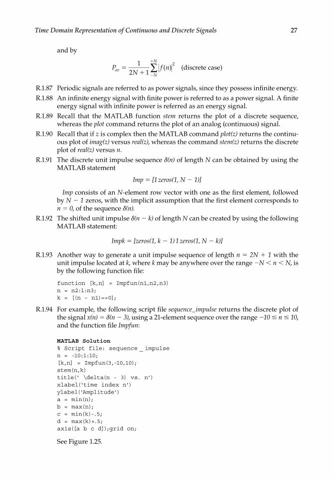
R.1.94 For example, the following script fi le sequence_impulse returns the discrete plot of the signal x(n) = δ(n − 3), using a 21-element sequence over the range −10 ≤ n ≤ 10, and the function fi le Impfun:
MATLAB Solution% Script file: sequence _ impulsen = -10:1:10;[k,n] = Impfun(3,-10,10);stem(n,k)title(‘ \delta(n - 3) vs. n’)xlabel(‘time index n’)ylabel(‘Amplitude’)a = min(n);b = max(n);c = min(k)-.5;d = max(k)+.5;axis([a b c d]);grid on;
See Figure 1.25.
CRC_47760_CH001.indd 27CRC_47760_CH001.indd 27 7/25/2008 4:16:15 PM7/25/2008 4:16:15 PM

28 Practical MATLAB® Applications for Engineers
R.1.95 A unit step sequence of length N can be generated using the following MATLAB command:
un = [ones(1, N)]
R.1.96 The shifted (or delayed) unit step sequence u(n − k) can be created by executing the following MATLAB command:
unk = [zeros(1, k − 1) ones(1, N)]
Observe that the total number of elements of the sequence unk is N + k − 1.R.1.97 The MATLAB function stepfun(n, no) returns the shifted step (by no units to the
right) sequence shown in Figure 1.26. Recall that the stepfun(n, no) can be used with either analog or discrete arguments, defi ned as
stepfun n no u n no
n no
n no( , ) ( )
10
forfor
1.5
1
0.5
−0.5−10 −8 −6 −4 −2 2 4 60
0
Am
plitu
de
8 10time index n
δ(n − 3) versus n
FIGURE 1.25Plot of x(n) = δ(n − 3) of R.1.94.
n0 n0+N
…
stepfun(n, n0)
n
FIGURE 1.26Plot of stepfun(n, no) of R.1.97.
CRC_47760_CH001.indd 28CRC_47760_CH001.indd 28 7/25/2008 4:16:15 PM7/25/2008 4:16:15 PM

Time Domain Representation of Continuous and Discrete Signals 29
The step function called Heaviside is indicated as follows:function stepseq = Heaviside(x)stepseq = (x>=0);
R.1.98 For example, write a program that returns u(t) and u(t − 2), using the function Heaviside, over the range −10 ≤ t ≤ 10.
MATLAB Solution>> x = -10:0.1:10;>> stepfun = Heaviside(x);>> subplot(2, 1, 1);>> plot(x, stepfun)>> xlabel(‘t (time)’)>> title(‘u(t) vs. t’)>> ylabel(‘Amplitude.’)>> axis([-10 10 ,0.5 1.5])>> subplot(2, 1, 2);>> stepfun = Heaviside(x-2);>> plot(x, stepfun)>> axis([-10 10 ,0.5 1.5])>> title(‘u(t-2) vs. t’)>> ylabel(‘Amplitude.’);>> xlabel(‘t (time)’);
See Figure 1.27.
R.1.99 The MATLAB function sign(t) is defi ned as follows:
sign t
t
t
t
( )
1 00 01 0
The sign(t) function is illustrated in Figure 1.28.
FIGURE 1.27Plots of u(t) and u(t − 2) of R.1.98.
1.5
Am
plitu
deA
mpl
itude
1
−10 −8 −6 −4 −2 0 2 4 6 8 100.5
1.5
1
0.5−10 −8 −6 −4 −2 0 2 4 6 8 10
t (time)
u(t) versus t
u(t − 2) versus t
t (time)
CRC_47760_CH001.indd 29CRC_47760_CH001.indd 29 7/25/2008 4:16:16 PM7/25/2008 4:16:16 PM

30 Practical MATLAB® Applications for Engineers
Note that the function sign(t) can be created by using the step functions indicated as follows:
sign(t) = u(t) − u(−t) = −1 + 2u(t)
R.1.100 The MATLAB symbolic toolbox calls the impulse function δ(t) by using the name Dirac(t).
R.1.101 The MATLAB symbolic toolbox calls the step function u(t) by using the name Heaviside(t).
R.1.102 The MATLAB symbolic toolbox calls the function sign(t) by using the name signum(t).
R.1.103 Let us gain some experience by using the MATLAB symbolic toolbox in evaluat-ing the following expressions:
a. δ( )t dt ∞
∞
∫b. u t dt( )
2
3
∫c. sign t dt( )
∞
∞
∫d. u t t( ) 3
e. u t t( ) 2
f. t u t dt( ) ∫g. t u t dt( )
1
2
∫h. t u t dt( )
1
2
∫i. t sign t dt( )
1
2
∫MATLAB Solution>> syms t a>> area _ impulse = int(‘Dirac(t)’, -inf, inf) % area of the impulse
δ(t)
area _ impulse = 1
>> area _ step = int(‘Heaviside(t)’, -2, 3) % area of the step from –2 to +3
sign(t)
t
1
0
−1
FIGURE 1.28Plot of the function sign(t) of R.1.99.
CRC_47760_CH001.indd 30CRC_47760_CH001.indd 30 7/25/2008 4:16:16 PM7/25/2008 4:16:16 PM

Time Domain Representation of Continuous and Discrete Signals 31
area _ step = 3
>> area _ sign = int(‘signum(t)’, -2, 3) % area of the sign from –2 to +3
area _ sign = 1
>> stept _ 3 = vpa(‘Heaviside(3)’) % evaluates u(t) at t =3
stept _ 3 = 1
>> stepmin _ 2 = vpa(‘Heaviside(-2)’) % returns u(t) at t = -2
stepmin _ 2 = 0
>> differstep = diff(‘Heaviside(t)’) % returns d(u(t))/dt
differstep = Dirac(t)
>> intramp = int(‘Heaviside(t)’*t) % returns the integral of t u(t) dt
intramp = 1/2*Heaviside(t)*t^2
>> area _ ramp12 = int(‘Heaviside(t)’*t,1,2) % area of [t u(t)] from t =1 to t =2
area _ ramp12 = 3/2
>> area _ ut _ 12 = int(‘Heaviside(t)’*t,-1,2) % area t u(t) from t = –1 to t =2
area _ ut _ 12 = 2
>> area _ signt = int(‘signum(t)’*t,-1,2) % area sign(t)*t from t=–1 to t=2
area _ sign = 5/2
R.1.104 Create the script fi le plot_ramp that returns the plot of t u(t) versus t, over the range −1 ≤ t ≤ 3, using ezplot.
MATLAB Solution% Script file: plot _ rampramp = (‘Heaviside(t)’*t) % returns the ramp over
–1 ≤ t ≤3ezplot(ramp, [-1 +3]) % see plot Figure 1.29title(‘heaviside(t)*t vs. t’);xlabel(‘t’); ylabel(‘t*u(t)’) ;
CRC_47760_CH001.indd 31CRC_47760_CH001.indd 31 7/25/2008 4:16:16 PM7/25/2008 4:16:16 PM

32 Practical MATLAB® Applications for Engineers
R.1.105 The MATLAB command square(t, a) returns the periodic square wave with period T = 2 * π, over the range defi ned by t, where a is a constant that indicates the per-cent of the period T for which the square wave is positive.
R.1.106 For example, create the script fi le squares that returns the plots over two cycles of the square sequences, with period T = 2π, with the following specs:a. f1(t) versus t, with mag[f1(t)] = 1, during 50% of the period T and mag[f1(t)] = −1,
during the remaining 50%b. f2(t) versus t, with mag[f2(t)] = 2, during 25% of the period T and mag[f2(t)] = −2,
during the remaining 75%c. f3(t) versus t, with mag[f3(t)] = 3, during 33% of the period T and mag[f3(t)] = −3,
during the remaining 67%d. f4(t) versus t, with mag[f4(t)] = 4, during 75% of the period T and mag[f4(t)] = −4,
during the remaining 25%
MATLAB Solution% Script file: squarest = 0:.1*pi:4*pi;f1 =square(t,50);f2 =2*square(t,25);f3 =3*square(t,33);f4 =4*square(t,75);subplot(2,2,1)plot(t,f1)ylabel(‘f1(t)’)axis([0 4*pi -1.5 1.5])grid on;title(‘Square(t,50) vs t’)subplot(2,2,2)plot(t,f2)
heaviside (t)*t versus t
3
2.5
2
1.5
1
0.5
0
−1 −0.5 0 0.5 1 1.5 2 2.5 3t
t*u(
t)
FIGURE 1.29Plot of t u(t) of R.1.104.
CRC_47760_CH001.indd 32CRC_47760_CH001.indd 32 7/25/2008 4:16:16 PM7/25/2008 4:16:16 PM

Time Domain Representation of Continuous and Discrete Signals 33
ylabel( ‘f2(t)’)axis([0 4*pi -2.5 2.5])grid on;title(‘2*Square(t,25) vs t’)subplot(2,2,3)plot(t,f3)axis([0 4*pi -4.5 4.5])grid on;ylabel(‘ f3(t) ‘);xlabel(‘ t (time)’)title(‘3*Square(t,33) vs t’)subplot(2,2,4)plot(t,f4)axis([0 4*pi -5.5 5.5])grid on;title(‘4*Square(t,75) vs t’)ylabel(‘ f4(t) ‘);xlabel(‘ t (time) ’)
The script fi le squares is executed and the results are shown in Figure 1.30.
R.1.107 The MATLAB command sawtooth(t, b) returns a triangular wave, with magni-tudes between −1 and +1, and a period of T = 2π. The scalar b, between 0 and 1, indicates the percent of the period T with positive slope, where the maximum occurs at the end.
Square(t,50) versus t
3*Square(t,33) versus t 4*Square(t,75) versus t
2*Square(t,25) versus t1.5
2
0
−1
−2
0 5 10
1
1
0.5
0
−0.5
−1
−1.50
4 5
0
0 5 10
−5
2
0
−2
−4
5 10
f1(t
)
f2(t
)
f3(t
)
f4(t
)
0 5 10
t (time)t (time)
FIGURE 1.30Plots of the function square of R.1.106.
CRC_47760_CH001.indd 33CRC_47760_CH001.indd 33 7/25/2008 4:16:17 PM7/25/2008 4:16:17 PM

34 Practical MATLAB® Applications for Engineers
R.1.108 For example, create the script fi le triangles that returns the plots over two cycles of the triangular sequences, with period T = 2π, with the following specs:a. f1(t) versus t, with positive slope during 50% of the period T, and a swing from
−1 to +1
b. f2(t) versus t, with positive slope during 25% of the period T, and a swing from −2 to +2
c. f3(t) versus t, with a positive slope during 33% of the period T, and a swing from −3 to +3
d. f4(t) versus t, with a positive slope during 75% of the period T, and a swing from −4 to +4
MATLAB Solution% Script file: trianglest = 0:0.1*pi:4*pi;f1 = sawtooth(t,.5);f2 = 2*sawtooth(t,.25);f3 = 3*sawtooth(t,.33);f4 = 4*sawtooth(t,.75);subplot(2,2,1)plot(t,f1)ylabel (‘f1(t)’)axis ([0 4*pi -1.5 1.5])grid on;title (‘Sawtooth(t,.50) vs t’)subplot(2,2,2)plot(t,f2)ylabel( ‘f2(t)’)axis ([0 4*pi -2.5 2.5])grid on;title (‘2*Sawtooth(t,.25) vs t’)subplot (2,2,3)plot (t,f3)axis ([0 4*pi -4.5 4.5])grid on;ylabel(‘ f3(t) ‘);xlabel(‘ t (time)’)title(‘3*Sawtooth(t,.33) vs t’)subplot(2,2,4)plot(t,f4)axis([0 4*pi -5.5 5.5])grid on;title(‘4*Sawtooth(t,.75) vs t’)ylabel(‘ f4(t) ‘); xlabel(‘ t (time) ’)
The script fi le triangles is executed and the results are shown in Figure 1.31.R.1.109 The MATLAB function sinc(x) evaluates the function defi ned by
sin ( )
sin( )c x
xx
R.1.110 For example, the script fi le sincs returns the plot of the function sinc(x) over the range 5 ≤ x ≤ 5, illustrated in Figure 1.32.
CRC_47760_CH001.indd 34CRC_47760_CH001.indd 34 7/25/2008 4:16:17 PM7/25/2008 4:16:17 PM

Time Domain Representation of Continuous and Discrete Signals 35
Sawtooth(t,.50) versus t 2*Sawtooth(t,.25) versus t1.5
0.5
0
0 5 10
−0.5
−1
−1.5
1
f1(t
)
f2(t
)
f3(t
)
3*Sawtooth(t,.33) versus t 4*Sawtooth(t,.75) versus t
2
1
0
0 5 10
−1
−2
5
−5
0
0 5 10
f4(t
)
t (time)
4
2
−2
−4
0
0 5 10
t (time)
FIGURE 1.31Plots of the function sawtooth of R.1.108.
FIGURE 1.32Plot of the function sinc of R.1.110.
sinc(x) versus x for −5 < x < 51
0.8
0.6
0.4
0.2
0
−0.2
−0.4−5 −4 −3 −2 −1 0 1 2 3 4 5
x
Am
plitu
de [S
inc(
x)]
CRC_47760_CH001.indd 35CRC_47760_CH001.indd 35 7/25/2008 4:16:17 PM7/25/2008 4:16:17 PM

36 Practical MATLAB® Applications for Engineers
MATLAB Solution% Script file: sincsx = -5:0.1:5;y = sinc(x);plot(x, y)title(‘sinc(x) vs. x for -5<x<5’)xlabel(‘x’);ylabel(‘Amplitude [Sinc(x)]’);grid on;
R.1.111 The MATLAB function tripuls(t, c) returns a symmetric triangle with its base along the horizontal axis, with length c, centered at t = 0.
R.1.112 For example, create the script fi le triang that returns the plots of triangles with the following specs:a. f1(t) versus t, with peak[f1(t)] = 1 and a base length = 3b. f2(t) versus t, with peak[f2(t)] = 2 and a base length = 5c. f3(t) versus t, with peak[f3(t)] = 3 and a base length = 10d. f4(t) versus t, with peak[f4(t)] = 4 and a base length = 12
MATLAB Solution% Script file: triangt = -6:0.1:6;f1 = tripuls(t,3);f2 = 2*tripuls(t,5);f3 = 3*tripuls(t,10);f4 = 4*tripuls(t,12);subplot(2,2,1)plot(t,f1)ylabel(‘Amplitude [f1(t)]’);xlabel(‘ t (time)’)axis([-6 6 -0.5 1.5])title(‘tripuls(t,3) vs. t’)subplot(2,2,2)plot(t,f2)ylabel( ‘Amplitude [f2(t)]’)xlabel(‘ t (time)’)axis([-6 6 -0.5 2.5])title(‘2*tripuls(t,5) vs. t’)subplot(2,2,3)plot(t,f3)axis([-6 6 -0.5 4.5])ylabel(‘ Amplitude [f3(t)] ‘);xlabel(‘ t (time)’)title(‘3*tripuls(t,10) vs. t’)subplot(2,2,4)plot(t,f4)axis([-6 6 -0.5 5.5])title(‘4*tripuls(t,12) vs. t’)ylabel(‘ Amplitude [f4(t)] ‘); xlabel(‘ t (time) ‘)
The script fi le triang is executed and the results are shown in Figure 1.33.R.1.113 The MATLAB function rectpuls(t, d) returns a symmetric rectangle with width d,
centered at t = 0.
CRC_47760_CH001.indd 36CRC_47760_CH001.indd 36 7/25/2008 4:16:17 PM7/25/2008 4:16:17 PM

Time Domain Representation of Continuous and Discrete Signals 37
R.1.114 For example, create the script fi le rect_pulses that returns rectangle plots with the following specs:a. f1(t) versus t, with mag[f1(t)] = 1 and width = 1
b. f2(t) versus t, with mag[f2(t)] = 2 and width = 3
c. f3(t) versus t, with mag[f3(t)] = 3 and width = 6
d. f4(t) versus t, with mag[f4(t)] = 4 and width = 9
MATLAB Solution% Script file: rect_ pulses t = -6:.1:6;f1 = rectpuls(t,1);f2 = 2*rectpuls(t,3);f3 = 3*rectpuls(t,6);f4 = 4*rectpuls(t,9);subplot(2,2,1)plot (t,f1)ylabel (‘ Amplitude [f1(t)]’);xlabel(‘t (time)’);axis ([-6 6 -0.5 1.5])title(‘Rectpuls(t,1) vs. t’)subplot(2,2,2)plot(t,f2)ylabel( ‘Amplitude [f2(t)]’); xlabel(‘t (time)’);axis([-6 6 -0.5 2.5])title(‘2*Rectpuls(t,3) vs. t’)subplot(2,2,3)
tripuls(t,3) versus t
3*tripuls(t,10) versus t
1.5
1
0.5
0
−0.5−5 0 5
Am
plitu
de [f
1(t)
]A
mpl
itude
[f3(
t)]
t (time)
Am
plitu
de [f
2(t)
]
2.5
2
1.5
1
0.5
−0.5−5 5
0
0
t (time)
2*tripuls(t,5) versus t
4*tripuls(t,12) versus t
5
4
3
2
1
0
−5 0 5
t (time)
Am
plitu
de [f
4(t)
]
4
3
2
1
−5 0 5
0 t (time)
FIGURE 1.33Plot of the function tripuls of R.1.112.
CRC_47760_CH001.indd 37CRC_47760_CH001.indd 37 7/25/2008 4:16:17 PM7/25/2008 4:16:17 PM

38 Practical MATLAB® Applications for Engineers
plot(t,f3)axis([-6 6 -0.5 4.5])ylabel(‘ Amplitude [f3(t)]’);xlabel(‘ t (time)’)title(‘3*Rectpuls(t,6) vs. t’)subplot(2,2,4)plot(t,f4)axis([-6 6 -0.5 5.5])title(‘4*Rectpuls(t,9) vs. t’)ylabel(‘ Amplitude [f4(t)] ‘); xlabel(‘ t (time) ‘)
The script fi le rect_pulses is executed and the results are shown in Figure 1.34.
R.1.115 The MATLAB function y = pulstran(t, d, ’f’) returns a symmetric train of continu-ous or discrete functions ‘f’ with d periods over the range defi ned by t.
R.1.116 A more general MATLAB function is [f, t] = gensig(‘type’, T, range, Ts) that returns the periodic function f defi ned by type (sin, square, or pulse), over the range t, with a sampling rate Ts.
R.1.117 For example, use the gensig command to create three cycles of a square periodic wave, with period T = 3 and a sampling rate Ts = 0.1 (Figure 1.35).
MATLAB Solution>> [squar,t] = gensig(‘square’,3,9,0.1);>> plot(t,squar)>> axis([0 9 0 1.2])>> ylabel(‘Amplitude’);xlabel(‘time’)>> title(‘Plot using [squar,t] = gensig(square,3,9,0.1)’)
Rectpuls(t,1) versus t 2*Rectpuls(t,3) versus t
4*Rectpuls(t,9) versus t3*Rectpuls(t,6) versus t
Am
plitu
de [f
2(t)
]A
mpl
itude
[f4(
t)]
1.5
1
0.5
0
−0.5−5 0 5
t (time)
t (time)
Am
plitu
de [f
1(t)
]
2.5
2
1.5
1
0.5
−0.5
5
4
3
2
1
0
0t (time)
−5 0 5
−5 50−5 50
t (time)
4
3
2
1
0
Am
plitu
de [f
3(t)
]
FIGURE 1.34Plots of the function rectpuls of R.1.114.
CRC_47760_CH001.indd 38CRC_47760_CH001.indd 38 7/25/2008 4:16:17 PM7/25/2008 4:16:17 PM

Time Domain Representation of Continuous and Discrete Signals 39
R.1.118 As an additional example, create the script fi le triang_pulses that returns the plots of triangular waves with 3, 4, 5, and 2 cycles, respectively, and unit magnitude, over the range 0 ≤ t ≤ 1.
MATLAB Solution% Script file: triang _ pulses% echo ont =0:0.001:1;subplot(2,2,1)d1 = [0:.33:1]; % 3 cycles y1 = pulstran(t,d1,’tripuls’,.25);plot (t,y1)title (‘3 triangular cycles’);axis ([0 1 -0.5 1.5]);ylabel(‘Amplitude’) ;subplot(2,2,2)da = [0:.25:1];y2 = pulstran(t,da,’tripuls’,.25); % 4 cyclesplot(t,y2);title(‘4 triangular cycles’);axis([0 1 -0.5 1.5]);ylabel(‘Amplitude’) ;subplot(2,2,3)d3 = [0:.20:1]; % 5 cyclesy3 = pulstran(t,d3,’tripuls’,.1);plot(t,y3);title(‘5 triangular cycles’);axis ([0 1 -0.5 1.5]); xlabel(‘time’)ylabel(‘Amplitude’) ;d4 = [0:.5:1]; % 2 cyclessubplot(2,2,4)y4 = pulstran(t,d4,’tripuls’,.4);plot (t,y4)
Plot using (squar, t) = gensig(square,3,9,0.1)
1
0.8A
mpl
itude
0.6
0.4
0.2
00 1 2 3 4 5 6 7 8 9
time
FIGURE 1.35Plot of R.1.117.
CRC_47760_CH001.indd 39CRC_47760_CH001.indd 39 7/25/2008 4:16:18 PM7/25/2008 4:16:18 PM

40 Practical MATLAB® Applications for Engineers
title (‘2 triangular cycles’);axis ([0 1 -0.5 1.5]);ylabel (‘Amplitude’) ;xlabel (‘time’);
The script fi le triang_pulses is executed and the results are shown in Figure 1.36.
R.1.119 Recall that system concepts such as transfer function, fi lter, and input and output signals were introduced in Chapter 7 of the book titled Practical MATLAB® Basics for Engineers.
The MATLAB command [h, t] = impulse(P, Q, t) returns as output h, when the input is a Dirac impulse applied to a fi lter or system whose transfer function is given by P/Q, where P and Q are polynomials expressed as row arrays whose coef-fi cients are arranged in descending order of s (where s = jw is the Laplace variable) and t is the time interval of interest (see Chapter 4 for more information).
R.1.120 The MATLAB command [gs, t] = step(P, Q, t) returns the step response of a linear system with a transfer function defi ned by H = P/Q, over a time interval t.
R.1.121 The MATLAB function hn = dimpulse(P, Q, n) returns the discrete impulse response consisting of n samples, applied to the discrete transfer function H(z) = P(z)/Q(z), where P(z) and Q(z) represent the vector polynomial consisting of its coeffi cients arranged in decreasing powers of z, where z = ejw.*
* See Chapter 5 for more information about z.
3 triangular cycles
5 triangular cycles
4 triangular cycles
2 triangular cycles
1.5
0.5
1.5 1.5
1
1
0.5
1
0
−0.5
0.5
−0.5
0
1
Am
plitu
deA
mpl
itude
Am
plitu
deA
mpl
itude
0
0
0.5
0.5
1
1
1.5
0.5
−0.50.5 1
0
0
1
0
0−0.5
0.5timetime
FIGURE 1.36Plots of R.1.118.
CRC_47760_CH001.indd 40CRC_47760_CH001.indd 40 7/25/2008 4:16:18 PM7/25/2008 4:16:18 PM

Time Domain Representation of Continuous and Discrete Signals 41
R.1.122 For example, let
H Z
z zz z
( ). . .
. .
2 24 2 5 2 250 5 0 68
2
2
Create the script fi le disc_imp that returns the discrete response in the form of a table and a plot for the sequence of length n = 10. The results are shown in Figure 1.37.
MATLAB Solution% Script file: disc _ impclc; clf;n =10;P = [2.24 2.5 2.25];Q = [1 .5 .68];hn = dimpulse(P,Q,n);nn = 0:1:9;results = [ nn’ hn];disp(‘*************************************************************’);disp(‘The impulse response sequence h(n) for the first 10 samples is:’);disp(‘ ^^^^^^^^^^^^^ ’);disp(‘ n h(n)’);disp(‘ ^^^^^^^^^^^^^ ’);disp(results);disp(‘*************************************************************’);yzero = zeros(1,10);stem(nn,hn); hold on; plot(nn,yzero)title(‘Discrete impulse response h(n) vs n’)xlabel(‘time index n’);ylabel(‘Amplitude [h(n)]’);
The script fi le disc_ imp is executed and the results are shown as follows:
********************************************************************The impulse response sequence h(n) for the first 10 samples is:^^^^^^^^^^^^^^^^^^^^^ n h(n)^^^^^^^^^^^^^^^^^^^^^ 0 2.2400 1.0000 1.3800 2.0000 0.0368 3.0000 -0.9568 4.0000 0.4534 5.0000 0.4239 6.0000 -0.5203 7.0000 -0.0281 8.0000 0.3679 9.0000 -0.1648********************************************************************
CRC_47760_CH001.indd 41CRC_47760_CH001.indd 41 7/25/2008 4:16:18 PM7/25/2008 4:16:18 PM

42 Practical MATLAB® Applications for Engineers
R.1.123 The MATLAB function un = dstep(P, Q, n) returns the discrete step response with length n of the system defi ned by the transfer function H(z) = P(z)/Q(z).
R.1.124 For example, create the script fi le disc_step that returns the discrete response in the form of a table and a plot for a sequence of length n = 10, for the system defi ned in R.1.122.
MATLAB Solution% Script file: disc _ stepclc; clf;n = 10;P = [2.24 2.5 2.25];Q = [1 .5 .68];un = dstep(P,Q,n);nn = 0:1:9;results = [nn’ un];disp(‘****************************************************************’);disp(‘The discrete step sequence u(n) for the first 10 samples is:’);disp(‘ ^^^^^^^^^^^^ ’)disp(‘ n u(n)’)disp(‘ ^^^^^^^^^^^^ ’)disp(results);disp(‘****************************************************************’);yzero = zeros(1,10);stem (nn,un); hold on; plot (nn,yzero)title (‘Discrete step response u(n) vs n’)xlabel (‘time index n’);ylabel (‘Amplitude[u(n)]’);
FIGURE 1.37Discrete impulse response h(n) of R.1.122.
Discrete impulse response h(n) versus n2.5
1.5
0.5
−0.5
1
0
0−1
1 2 3 4 5 6 7 8 9
2A
mpl
itude
[h(n
)]
time index n
CRC_47760_CH001.indd 42CRC_47760_CH001.indd 42 7/25/2008 4:16:18 PM7/25/2008 4:16:18 PM

Time Domain Representation of Continuous and Discrete Signals 43
The script fi le disc_step is executed and the results are given as follows and in Figure 1.38.
*****************************************************************The discrete step sequence u(n) for the first 10 samples is:^^^^^^^^^^^^^^^^^^^^ n u(n)^^^^^^^^^^^^^^^^^^^^ 0 2.2400 1.0000 3.6200 2.0000 3.6568 3.0000 2.7000 4.0000 3.1534 5.0000 3.5773 6.0000 3.0570 7.0000 3.0289 8.0000 3.3968 9.0000 3.2320*****************************************************************
R.1.125 The MATLAB function [y, n] = fi lter(b, a, x) defi ned in Chapter 7 of the book titled Practical MATLAB® Basics for Engineers returns the output sequence y, when the relation input (x) output (y) is given by the following system difference equation:
a y n k b x n lk
k
N
ll
N
= =∑ ∑
0
1
0
2
( ) ( )
R.1.126 A discrete sequence may consist of either a fi nite or infi nite number of samples. A fi nite length sequence is characterized by a fi nite number of nonzero sam-ples. An infi nite length sequence extends infi nitely to the right or the left of the n-axis (discrete time). In either case, the infi nite or fi nite sequences can be represented by a sum of weighted time-shifted impulse samples.
Discrete step response u(n) versus n4
3.5
2.5
2
1.5
0.5
00 1 2 3 4 5 6 7 8 9
1
3
time index n
Am
plitu
de [u
(n)]
FIGURE 1.38Discrete step response of R.1.124.
CRC_47760_CH001.indd 43CRC_47760_CH001.indd 43 7/25/2008 4:16:18 PM7/25/2008 4:16:18 PM

44 Practical MATLAB® Applications for Engineers
R.1.127 Reconstruction of an analog signal f(t) from the discrete sequence f(n) can be accomplished, if the analog signal f(t) is band-limited and converted into the dis-crete sequence f(n) by sampling it with a rate above the Nyquist/Shannon rate.
R.1.128 Recall that the sampling theorem (Nyquist/Shannon) states that an analog signal f(t), band-limited to fm hertz, must be sampled at a rate greater than twice its high-est frequency fm, to be able to reconstruct f(t) from its samples given by f(n) (R.1.1).
The reconstruction process is done by passing the sequence f(n) through an ideal analog low-pass fi lter with a cutoff frequency of fm (see Chapters 4 and 6 for infor-mation regarding frequency domain and fi ltering).
R.1.129 Since ideal sharp rectangular fi lters, with a cutoff frequency of fm are unrealiz-able, the practical sampling rate is often fi ve or six times the frequency fm. At this point let us analyze the reconstruction process in the time domain, where the reconstructed signal f(t) can be approximated by the following equation:
f t f n
c t nTTn
n
( ) ( )sin ( )
∑
where
sin ( )
sin( )c t
tt
R.1.130 If a discrete time signal f(n) was originally obtained by sampling a band-limited continuous time signal by using the Nyquist/Shannon sampling rate, then the process of up- or down-sampling the time continuous signal f(t) means that the original signal is sampled now by a higher or lower sampling rate.
R.1.131 The term up-sampling refers to increasing the sampling rate by an integer factor L. This process means that interpolation is required by placing additional samples between the original sampled function f(n). This process is accomplished by a low-pass fi lter scaled to a cutoff frequency wc = π/L.
R.1.132 The MATLAB function interp returns the sequence fL that consists of increasing the sequence f(n) defi ned by a vector f by an integer factor L.
The function interp can take any of the following forms: a. fL = interp(f, L)
b. fL = interp(f, LN, a)
c. [fL, h] = interp(f, L,N, a) (with default values of L = 4 and a = 0.5)The resampled vector fL has a length given by length(fL) = L * length(f).
The sample signal f is assumed to be band-limited scaled to 0 ≤ w ≤ a, with a ≤ 0.5, where h represents the interpolation fi lter coeffi cient. Ideally L ≤ 10.
R.1.133 The term decimate is referred to the reduction or down-sampling the discrete sig-nal f by an integer factor M, returning the sequence fM.
The MATLAB function decimate can take any of the following forms:
fM = decimate(f, M)
fM = decimate(f, M . n)
fM = decimate(f, M . ’fi r’)
fM = decimate(f, M, N, ’fi r’)
CRC_47760_CH001.indd 44CRC_47760_CH001.indd 44 7/25/2008 4:16:18 PM7/25/2008 4:16:18 PM

Time Domain Representation of Continuous and Discrete Signals 45
wheref is the input sampled vector (f(n)).M the down-sampling integer rate factor, or the resampling rate is 1/M times the
original rate. The resulting length is given by length(fM) = [length (f)]/M.N the order of the (Chebyshev type-1) fi lter used to accomplish the resampling.fi r a 30-point low-pass fi lter forward direction only with cutoff frequency wc = π/M,
before resampling is done.The decimation process of the fi rst two options uses an IIF Chebyshev low-pass
type-1 fi lter with forward and backward directions (see Chapter 6 for information regarding fi lters).
R.1.134 The MATLAB function resample returns the sequence f LM, consisting of f resa-mpled with a rate that is the ratio of two integers given by L/M.
The syntax of the function resample with some options is indicated as follows:
fLM = resample(f, L, M)
fLM = resample(f, L, M, R)
fLM = resample(f, L, M, h)
[fLM, h] = resample(f, L, M)
where R is the input rate with a default value of 10. This function uses an FIR, and a Kaiser window with β = 5 (windows are presented later in this section).
R.1.135 The process referred to as multiplexing consists of merging two (or more) discrete sequences f1(n) and f2(n) into a single sequence by alternating the samples of f1(n) with f2(n). Then the resulting multiplexed, or in short mux sequence is given by
mux(f1, f2) = [f1(1) f2(1) f1(2) f2(2) f1(3) f2(3) … f1(n − 1) f2(n − 1) f1(n) f2(n)]
The lengths of the sequences of f1 and f2 are assumed to be n (equal). Then the length of mux (f1, f2) sequence is 2n. If the sequences are f1(n) and f2(m), where n > m, then by increasing the length of f2 to n, by making the last n − m samples zeros, the two sequences (lengths) became equal and the mux command can then be safely used.
R.1.136 Signals may also be classifi ed according to the probability of predicting its behav-ior with certainty or with some sort of ambiguity intoa. Deterministic or nonrandomb. Probabilistic, stochastic, or random
R.1.137 Deterministic signals can be expressed in terms of a well-defi ned process, table, rules, or by a mathematical relation (equation). These type of signals are fully predictable.
R.1.138 Random signals are not predictable; they are noise-like functions where particular values or samples are not important, but rather the statistical information over a large range of samples is, such as the expected value, the mean, and standard deviation. Most signals encountered in practical applications and in this text are real and deterministic. Observe that random signals cannot be reproduced, but may carry valuable information. The more unpredictable or random a signal is the more information it carries.
CRC_47760_CH001.indd 45CRC_47760_CH001.indd 45 7/25/2008 4:16:18 PM7/25/2008 4:16:18 PM

46 Practical MATLAB® Applications for Engineers
R.1.139 The process of limiting or truncating a function or sequence consisting of an infi -nite or a very large number of samples such as
f n F n ll
l
( ) ( )
∑
is by approximating f(n) by another fa(n), consisting of a fi nite number of samples (2N + 1) given by
f n F n la l
l N
N
( ) ( )
∑
Mathematically, the truncation process is accomplished by multiplying the function f(n) by another function w(n) called rectangular window, where w(n) is defi ned by
w n
n N
n N( )
| || |
10
Observe that the lengths of w(n) and fa(n) are 2N + 1. The rectangular window is the simplest model used to truncate a function and all the weighing coeffi cients used for that purpose are one. Note that w(n) is equivalent to the pulse function pul(n/N).
R.1.140 The practical way to deal with a function f(n), which has an infi nite range, is by truncating f(n). Therefore,
fa(n) = f (n) * w(n)
An additional objective of w(n) is to improve the smoothness of fa(n) by removing oscillations associated with a sharp truncation process.
R.1.141 Practical considerations of the truncation process and the use of different window models are better understood in the frequency domain with applications in fi lter design (see Chapters 4 and 6).
R.1.142 Many window models have been proposed by mathematicians and engineers over the last century. All the window models share similar properties such asa. The sample located at n = 0 is multiplied (scaled) by 1 (unaffected).b. The shape of f(n) is relatively unaffected for n < |N|.
c. The shape of f(n) is increasingly affected for the values of n in the vicinity of |N|.
d. The window coeffi cients range from 1 to 0, where 1 corresponds to the value at n = 0 and the smaller coeffi cients are for the larger values of n as n approaches N.
e. All window models are of fi nite length and the point of symmetry is located at the midpoint [length (w(n))]/2.
R.1.143 When an arbitrary function presents a discontinuity and is approximated by a large, but fi nite number of terms, a ripple is generated at the discontinuity with a magnitude of about 10% of the jump value. This behavior is referred to as the Gibb’s phenomenon (see Chapter 4 for more details). The objective of the various window models is to reduce the Gibb’s effect that translates into oscillations.
CRC_47760_CH001.indd 46CRC_47760_CH001.indd 46 7/25/2008 4:16:19 PM7/25/2008 4:16:19 PM

Time Domain Representation of Continuous and Discrete Signals 47
R.1.144 MATLAB offers the user a number of built-in window functions in the signal pro-cessing toolbox. Some of the window models most often used are known by the following names: a. Rectangularb. Triangularc. Hanningd. Hamminge. Kaiserf. Chebyshevg. Bartletth. Blackman
R.1.145 The MATLAB function Hamming(N) returns a vector with N-weighted points referred to as the Hamming window.
R.1.146 Similarly, the MATLAB commandsHanning(N)
Blackman(N)
return N-length vectors representing the Hanning or Blackman weighted-type windows.
R.1.147 The three window models: Hamming, Hanning, and Blackman are based on cosine functions. The mathematical equations used to generate the above window sequences are defi ned as follows:a. For the Hamming window,
w(n) = 0.54 + 0.46 cos( * n/M)
b. For the Hanning (Van Hann) window, w(n) = 0.54 + 0.46 cos(( * n)/(M + 1))
c. For the Blackman window, w(n) = 0.5 + 0.46 cos(( * n)/M) + 0.08 cos((4 * * n)/(2n + 1))
where M = 1/2(L − 1) is an integer representing the midpoint and L is the window’s length.
R.1.148 The MATLAB command Kaiser (N, β) returns the N points of the Kaiser window, where β is a constant, with the following range 1 ≤ β ≤ 10, where β represents a tradeoff between the side lobe height and its width. The Kaiser window is based on the modifi ed Bessel function Io(x) given as follows:
w n
I n M MI
n Lo
O
( )( ) /
( ), , , ( )
10 1 2 1
2 for … −
where M = 1/2(L − 1) is the midpoint and the weight β is over the range 0 ≤ β ≤ 10.
This window is frequently used in the design of fi lters, where β controls the stop- and pass-band ripples.
R.1.149 The MATLAB function triang(N) returns the N-point triangular window based on the following equation:
w n
nM
( ) 11
CRC_47760_CH001.indd 47CRC_47760_CH001.indd 47 7/25/2008 4:16:19 PM7/25/2008 4:16:19 PM

48 Practical MATLAB® Applications for Engineers
R.1.150 The MATLAB function boxcar(N) returns the N points of a rectangular window defi ned by
w n
n M
n M( )
| || |
10
R.1.151 The MATLAB function Bartlett(N) returns the N points of the Bartlett window based on the equation
w n
M nM
( )
R.1.152 There are other popular window models such as Parabolic, Cauchy, and Gaussian defi ned below. The Parabolic or Parzen window is based on the equation given by
w n
n MM
( ) 12
R.1.153 The Cauchy window is defi ned by the equation given by
w n
MM n M
( )( )
2
2 2 2
where α is an optional control character.R.1.154 The Gaussian window is defi ned by the following equation:
w n
n MM
( ) exp 1
22
2
where α is an optional control character.R.1.155 All the proposed window models share the characteristic that the peak occurs in
the middle (midpoint) of the window sequence, whereas at its edges (end points) the behavior tends to be smooth.
The behavior of some of the window models may present side lobes or undesir-able shapes over some regions. In any case, an attempt is made to present only the most important and the widely accepted window models without exploring their behaviors.
R.1.156 For example, create the script fi le windows that returns the plots of the following windows:a. Hamming
b. Hanning
c. Blackman
shown in Figure 1.39, using N = 31.
MATLAB Solution>> n = -15:1:15;>> WHAM = Hamming(31);>> WHAN = Hanning(31);>> WBLAC = Blackman(31);
CRC_47760_CH001.indd 48CRC_47760_CH001.indd 48 7/25/2008 4:16:19 PM7/25/2008 4:16:19 PM

Time Domain Representation of Continuous and Discrete Signals 49
>> subplot(3, 1, 1);>> plot(n, WHAM);>> title(‘Hamming(31) window’);>> ylabel(‘Amplitude’);xlabel(‘n’)>> subplot(3, 1, 2);>> plot(n, WHAN);>> title(‘Hanning(31) window’);>> ylabel(‘Amplitude’);xlabel(‘n’)>> subplot(3, 1, 3);>> plot(n, WBLAC);>> title(‘Blackman(31) window’);>> xlabel(‘n’);>> ylabel(‘Amplitude’)
R.1.157 Observe that the Hamming, Hanning, and Blackman window models shown in Figure 1.39 present similar shapes. They are plotted on the same graph for com-parison purposes in Figure 1.40, given by script fi le compare_win.
MATLAB Solution% Script file:compare _ win% This file returns the plots of the % HAMMING, HANNING and BLACKMAN windows% using 31 points.%*******************************clc;clf;n = -15:1:15;
Blackman (31) window
−15 −10 −5 0 5 10
n
15
1
0.5
−15 −10 −5 0 5 10 150
Hamming (31) window
Hanning (31) window
1
0.5
−15
1
−10 −5 0 5 10 150
Am
plitu
deA
mpl
itude
Am
plitu
de
n
n
0.5
0
FIGURE 1.39Plots of the Hamming, Hanning, and Blackman windows of R.1.156.
CRC_47760_CH001.indd 49CRC_47760_CH001.indd 49 7/25/2008 4:16:19 PM7/25/2008 4:16:19 PM

50 Practical MATLAB® Applications for Engineers
wham = hamming(31);whan = hanning(31);wblac = blackman(31);plot(n,wham,’*’,n,whan,’d’,n,wblac,’o’);holdplot(n,wham,n,whan,n,wblac);title(‘HAMMING,HANNING and BLACKMAN windows ‘);xlabel(‘points n’);ylabel(‘Amplitude’)legend(‘HAMM’,’HANN’,’BLAC’);
R.1.158 The Kaiser window is a controllable window (controlled by β), and is presented as follows, by the script fi le Kaisers for the following values of β: 3, 7, and 10, using an N = 31-point approximation.
MATLAB Solution% Script file: Kaisers% This file returns the plots % KAISER window for betas: 3,7,10.% using a 31 point approximation%*******************************clc;clf;n = -15:1:15;wk3 = kaiser(31,3);wk7=kaiser(31,7);
HAMMING, HANNING, and BLACKMAN windows1
0.9
0.8
0.7
0.6
0.5
0.4
0.3
0.2
0.1
0−15 −10 −5 0 5 10 15
points n
HammHann
Blac
Am
plitu
de
n
n
FIGURE 1.40Plots of Hamm, Hann, and Blackman windows of R.1.157.
CRC_47760_CH001.indd 50CRC_47760_CH001.indd 50 7/25/2008 4:16:19 PM7/25/2008 4:16:19 PM

Time Domain Representation of Continuous and Discrete Signals 51
wk10 = kaiser(31,10);plot(n,wk3,’*’,n,wk7,’d’,n,wk10,’o’);holdplot(n,wk3,n,wk7’,n,wk10);title(‘KAISER windows for \beta=3,7, and 10 ‘);xlabel(‘points n’);ylabel(‘Amplitude’)legend(‘\beta:3’,’\beta:7’,’\beta:10’);
The script fi le Kaisers is executed and the resulting plots are shown in Figure 1.41.Observe from Figure 1.41 that the larger the β the sharper the shape.
R.1.159 The script fi le win_tri_rect_bar returns the plots of the triangular, rectangular, and Bartlett window plots using an N = 31 approximation. The resulting plots are shown in Figure 1.42.
MATLAB Solution% Script file: win _ tri _ rect _ bar% This file returns the plots of the % TRIANGULAR, RECTANGULAR and % BARTLETT windows% using a 31 point approximation%**************************************clc; clf;n = -15:1:15;
KAISER windows for β=3, 7, and 101
0.8
0.7
0.6
0.5
0.4
0.3
0.2
0.1
0
0.9
−15 −10 −5 0 5 10 15
Am
plitu
de
β:3
β:7
β:10
points n
FIGURE 1.41Plots of the Kaiser windows of R.1.158.
CRC_47760_CH001.indd 51CRC_47760_CH001.indd 51 7/25/2008 4:16:19 PM7/25/2008 4:16:19 PM
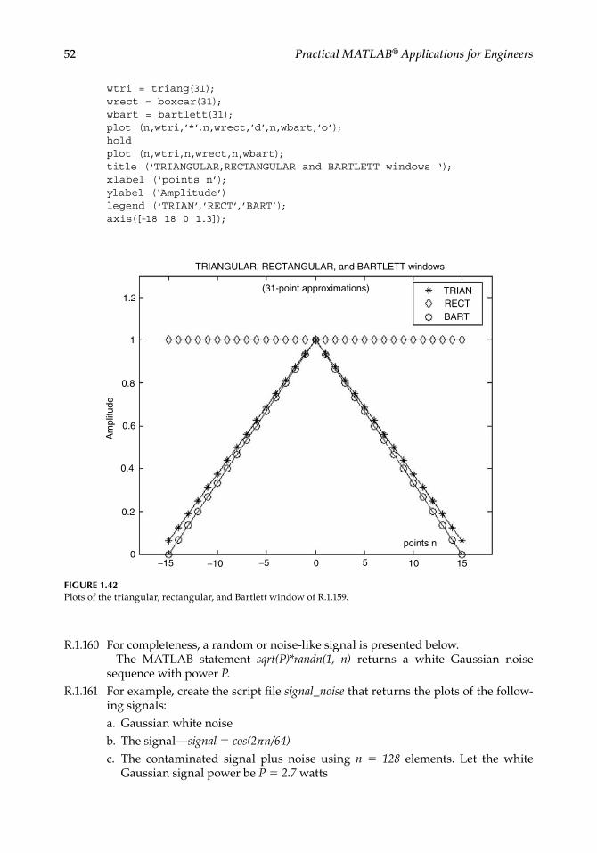
52 Practical MATLAB® Applications for Engineers
wtri = triang(31);wrect = boxcar(31);wbart = bartlett(31);plot (n,wtri,’*’,n,wrect,’d’,n,wbart,’o’);holdplot (n,wtri,n,wrect,n,wbart);title (‘TRIANGULAR,RECTANGULAR and BARTLETT windows ‘);xlabel (‘points n’);ylabel (‘Amplitude’)legend (‘TRIAN’,’RECT’,’BART’);axis([-18 18 0 1.3]);
R.1.160 For completeness, a random or noise-like signal is presented below.The MATLAB statement sqrt(P)*randn(1, n) returns a white Gaussian noise
sequence with power P.R.1.161 For example, create the script fi le signal_noise that returns the plots of the follow-
ing signals: a. Gaussian white noiseb. The signal—signal = cos(2πn/64)
c. The contaminated signal plus noise using n = 128 elements. Let the white Gaussian signal power be P = 2.7 watts
TRIANGULAR, RECTANGULAR, and BARTLETT windows
1.2
1
0.8
0.6
0.4
0.2
0−15 −10 −5 0 5 10 15
Am
plitu
de
TRIANRECTBART
(31-point approximations)
points n
FIGURE 1.42Plots of the triangular, rectangular, and Bartlett window of R.1.159.
CRC_47760_CH001.indd 52CRC_47760_CH001.indd 52 7/25/2008 4:16:20 PM7/25/2008 4:16:20 PM

Time Domain Representation of Continuous and Discrete Signals 53
MATLAB Solution% Script file: signal _ noisen = 1:128; P =2.7;figure(1)subplot(2,1,1)white _ noise = sqrt(P)*randn(1,128);stem(n,white _ noise); hold on;plot(n,white _ noise);xlabel(‘discrete time n’);ylabel(‘Amplitude’); title(‘Gaussian noise’);subplot(2,1,2)signal = cos(2*pi*n/64);stem(n,signal);hold on;plot(n,signal);title(‘cosine wave with period=64’)xlabel(‘discrete time n’);ylabel(‘Amplitude’);
figure(2)signal _ noise = white _ noise+signal;stem(n,signal _ noise);hold on;plot(n,signal _ noise);title(‘cosine wave plus white Gaussian noise’)xlabel(‘discrete time n’);ylabel(‘Amplitude’);
The script fi le signal_noise is executed as follows and the results are shown in Figures 1.43 and 1.44.
FIGURE 1.43Plots of parts a and b of R.1.161.
Gaussian noise4
2
0
−2
−40 40 60 80 100 120 14020
Am
plitu
deA
mpl
itude
discrete time n
cosine wave with period = 641
0.5
0
−0.5
−10 20 40 60 80 100 120 140
discrete time n
CRC_47760_CH001.indd 53CRC_47760_CH001.indd 53 7/25/2008 4:16:20 PM7/25/2008 4:16:20 PM

54 Practical MATLAB® Applications for Engineers
R.1.162 Sound waves can be represented by 1-D vectors while 2-D matrices can be used to represent images (black and white), whereas higher dimension matrices can be used to represent color images and video.
R.1.163 The MATLAB command wavrecord(N, Fs) takes the N audio elements sampled at a frequency of Fs, directly from an audio input device such as a microphone. The default value for Fs is 11,025 Hz. This function can only be used with Windows 95, 98, or NT machines.
R.1.164 The MATLAB command wavplay(y, Fs) sends the audio signal defi ned by the vector y, sampled at a frequency of Fs Hertz to an output audio device. Standard audio rates are 8000, 11,025, 22,050, and 44,100 Hz. The MATLAB default rate is 11,025 Hz.
R.1.165 MATLAB provides with a sound fi le called sound(y, Fs), and soundsc(y, Fs), that sends the audio signal defi ned by y to an output audio device. y is assumed to have a magnitude range −1.0 ≤ y ≤ 1.0, and any values outside that range is clipped. The difference between sound and soundsc is that the latter is autoscale, and y is played as loud as possible. The MATLAB default sound rate is 8192 Hz.
MATLAB also provides with a speech fi le named mtlb.mat that can be used for testing purposes, consists of 4001 elements, sampled at 1418 Hz.
R.1.166 The following example shows the script fi le audio that returnsa. The plot of the sinusoidal audio signal is given by y = cos(2πfot) + 3 cos(0.5πfot);
where fo = 1000 Hz, and a sample frequency of Fs = 8000 Hz (implying that 8000 audio samples per second are processed).
b. The speech fi le mtlb (Figure 1.45).
cosine wave plus white Gaussian noise5
4
3
2
1
0
−1
−2
−3
−4
−50 20 40 60 80 100 120 140
discrete time n
Am
plitu
de
FIGURE 1.44Plot of part c of R.1.161.
CRC_47760_CH001.indd 54CRC_47760_CH001.indd 54 7/25/2008 4:16:20 PM7/25/2008 4:16:20 PM

Time Domain Representation of Continuous and Discrete Signals 55
MATLAB Solution% Script file: audiosubplot(2,1,1)fo = 1000;Fs = 8000;Ts =1/Fs;t = 0:Ts:1;y = cos(2*pi*fo.*t)+3*cos(0.5*pi*fo.*t); % audio sequenceplot(t(1:100),y(1:100));ylabel(‘Amplitude’);xlabel(‘time (sec)’);title(‘cos(2\pi fo t)+3 cos(0.5\pi fo t) vs.t ‘)
subplot(2,1,2)load mtlb; Fs=1418; T=1/Fs;x = 1:4001;xx=x.*T; % speech fileplot(xx,mtlb);axis([0 4000*T -4 4]);ylabel(‘Amplitude ‘);title(‘[Speech file mtlb] vs. t’);xlabel(‘time (sec)’)
R.1.167 The MATLAB command [y, Fs, nbits] = wavread(‘microsoft_fi le’) returns the vector y consisting of the audio wave samples from a Microsoft fi le, at a sampling frequency Fs, using n bits to encode each sample of y, whereas the amplitude of y is scaled over the range −1 ≤ y ≤ +1. Similarly, the command wavwrite returns a Microsoft wave fi le.
R.1.168 The MATLAB command image(matrix_A) returns matrix_A as an image, where each element of the matrix_A is defi ned by a color. The matrix dimensions may be 2-D (m × n) or 3-D (m × n × r). In its simplest version, the elements of the 2-D (n × m) matrix are used as indices in the current colormap to defi ne its color.
FIGURE 1.45Plots of audio and speech fi les of R.1.166.
cos (2π fo t) + 3 cos (0.5π fo t) versus t4
2
0
−2
−40 0.002 0.004 0.006 0.008 0.01 0.012 0.014
time (sec)
time (sec)
[Speech file mtlb] versus t4
2
0
−2
−40 0.5 1 1.5 2 2.5
Am
plitu
deA
mpl
itude
CRC_47760_CH001.indd 55CRC_47760_CH001.indd 55 7/25/2008 4:16:20 PM7/25/2008 4:16:20 PM

56 Practical MATLAB® Applications for Engineers
R.1.169 For example, the color image of the magic(10) matrix is processed and displayed as follows, Figure 1.46:
MATLAB Solution>> image(magic(10))>> title(‘Image of the magic(10) matrix’)
R.1.170 Images can be transformed and processed by the fi ltering functions presented in Chapter 6. In general, the fi ltering process involves sophisticated mathematical manipulations, that rely on the theory of complex variables and transform theory.
Precisely for these reasons MATLAB provides its users with simple fi ltering commands, avoiding all the complicated mathematics used on image processing defi ned for 2-D matrices such as gradianr(matrix_A) and del1(matrix_A).
The command gradianr(matrix_A) returns the numerical gradient, whereas the command del1(matrix_A) returns its derivative (the discrete Laplacian).
R.1.171 Let us illustrate some of the image processing techniques by performing the fi rst and second derivative using as an illustrative example, the matrix y = magic(10). The results are shown in Figures 1.47 and 1.48.
MATLAB Solutiony = magic(10);>> ygrad = gradient(y); >> figure(1);>> image(ygrad)>> title(‘gradient of magic(10)’)>> ydel2 = del2(y); >> figure(2);>> image(ydel2)>> title(‘second derivative (del2) of magic(10)’)
R.1.172 Animation and motion of video signals can be accomplished using MATLAB by displaying pictures or fi gures one after the other, referred to as frames.
R.1.173 The MATLAB command getframe captures the content of the current fi gure win-dow and creates with it a movie frame. The getframe command is placed usually
FIGURE 1.46(See color insert following page 374.) Color plot of the magic matrix of R.1.169.
Image of the magic (10) matrix
1
2
3
4
5
6
7
8
9
10
1 2 3 4 5 6 7 8 9 10
CRC_47760_CH001.indd 56CRC_47760_CH001.indd 56 7/25/2008 4:16:21 PM7/25/2008 4:16:21 PM

Time Domain Representation of Continuous and Discrete Signals 57
in a ( for-end) loop, to assemble an array of movie frames, spaced over time by its looping index.
R.1.174 For example, the following MATLAB sequence can be used to assemble a movie, based on the contents of the current fi gure window over n.
MATLAB Solutionfor frame=1:n M(frame) = getframe; % captures the current figure as a frame
of Mend
R.1.175 The MATLAB command movie(M) displays the recorded M array containing all the frames of M, one frame after the other in sequential ascending order: frame(1), frame(2), frame(3), …, frame(n − 1), frame(n).
FIGURE 1.47(See color insert following page 374.) First color derivative plot of the magic matrix of R.1.169.
gradient of magic (10)
1
2
3
4
5
6
7
8
9
10
1 2 3 4 5 6 7 8 9 10
FIGURE 1.48(See color insert following page 374.) Second color derivative plot of the magic matrix of R.1.169.
second derivative (deI2) of magic(10)
1
2
3
4
5
6
7
8
9
10
1 2 3 4 5 6 7 8 9 10
CRC_47760_CH001.indd 57CRC_47760_CH001.indd 57 7/25/2008 4:16:21 PM7/25/2008 4:16:21 PM

58 Practical MATLAB® Applications for Engineers
1.4 Examples
Example 1.1
Create the script fi le disc_func that returns the plot of the following discrete function (Figure 1.49):
ƒ(n) = −5(n + 4) + (n) + 2(n − 3)
MATLAB Solution% Script file : disc _ func n = -10:10; % vector n from -10 to +10fn = [zeros(1,6) -5 zeros(1,3) 1 zeros(1,2) 2 zeros(1,7)];yzero = zeros(1,21);% plot the function f(n)stem(n,fn) % plot the function f(n)hold on;plot(n,yzero);xlabel(‘time index, n’)ylabel(‘Amplitude’)axis([-10 10 -7 4])title(‘f(n) = -5\delta(n+4) + \delta(n) +2\delta(n-3)’)
Example 1.2
Create the script fi le analog_func that returns the plot of the analog signal given by
ƒ(t) = u(t) + u(t − 1) + u(t − 2) − 3u(t − 3)
over the range −1 ≤ t ≤ 5 (Figure 1.50).
f(n) = −5δ(n+4) + δ(n) + 2δ(n−3)4
3
2
1
−1
−2
−3
−4
−5
−6
−10 −8 −6 −4 −2 0 2 4 6 8 10−7
0
time index, n
Am
plitu
de
FIGURE 1.49Plot of Example 1.1.
CRC_47760_CH001.indd 58CRC_47760_CH001.indd 58 7/25/2008 4:16:22 PM7/25/2008 4:16:22 PM

Time Domain Representation of Continuous and Discrete Signals 59
MATLAB Solution% Script file: analog _ funct = -1:0.01:5;t0 = 0;ut = stepfun(t,t0); % u(t)t0 =1;ut1 =stepfun(t,t0); % u(t-1)t0 = 2;ut2 = stepfun(t,t0); % u(t-2)t0 = 3;ut3 = -3 * stepfun(t,t0); % -3u(t-3)fn = ut+ut1+ut2+ut3;plot(t,fn);axis([-1 5 -1 4])title(‘f(t) = u(t) + u(t-1) + u(t-2) - 3u(t-3) ‘)xlabel(‘time t’)ylabel(‘Amplitude [f(t)]’)
The script fi le analog-func is executed and the result is shown in Figure 1.50.
Example 1.3
Create the script fi le sequences that uses MATLAB to verify graphically that the discrete sequences f1(n) and f2(n), defi ned as follows, over the range −10 ≤ n ≤ 10 are equal:
ƒ1(n) = 3 u(−n) * u(n + 5)
and
ƒ2(n) = 3[u(n + 5) − u(n + 1)]
MATLAB Solution% Script file: sequencesclc; clf;yzero = [zeros(1,21)]; n=-10:10;n0 = 0;un = stepfun(n, n0);
FIGURE 1.50Plot of Example 1.2.
−1 0 1 2 3 4 5−1
−0.5
0
0.5
1
1.5
2
2.5
3
3.5
4f(t) = u(t) + u(t−1) + u(t−2) − 3u(t−3)
time (t)
Am
plitu
de [
f(t)
]
CRC_47760_CH001.indd 59CRC_47760_CH001.indd 59 7/25/2008 4:16:22 PM7/25/2008 4:16:22 PM

60 Practical MATLAB® Applications for Engineers
urev = fliplr(un);n1 = -5;un _ 5 = stepfun(n, n1); fn1=3*(urev .* un _ 5);subplot(2,1,1)stem(n,fn1);hold on; plot(n,yzero)title(‘f1(n) vs. n’);ylabel(‘Amplitude [f1(n)]’); xlabel(‘Discrete time n’)un1=stepfun(n,1); fn2=3*(un _ 5 -un1);axis([-10 10 -1 4])subplot(2,1,2)stem(n, fn2);hold on; plot(n,yzero);title(‘f2(n) vs. n’); ylabel(‘Amplitude [f1(n)]’); xlabel(‘ Discrete time n ‘);axis([-10 10 -1 4])
The script fi le sequences is executed and the results are shown in Figure 1.51.
Example 1.4
Create the script fi le graphs that returns the plots of the following time functions:
f t e t u tt1
1 44 5 8 3 1 25( ) . cos( . . ) ( ).
and
f2(t) = f1(–t)
over the range −5 ≤ t ≤ 5.
FIGURE 1.51Plots of Example 1.3.
f1(n) versus n
f2(n) versus n
4
3
2
1
−1−10 −8 −6 −4 −2 0 2 4 6
Discrete time n
8 10
0Am
plitu
de [f
1(n)
]A
mpl
itude
[f2(
n)]
4
3
2
1
0
−1−10 −8 −6 −4 −2 0 2 4 6 8 10
Discrete time n
CRC_47760_CH001.indd 60CRC_47760_CH001.indd 60 7/25/2008 4:16:23 PM7/25/2008 4:16:23 PM

Time Domain Representation of Continuous and Discrete Signals 61
MATLAB Solution% Script file: graphst = -5:.01:5; t0 = 0;u = stepfun(t,t0);f1 = 4.5*exp(-1.4.*t).*cos(8.3.*t+1.25).*u;subplot(2,1,1);plot(t,f1);axis([-5 5 -4 5]);title(‘[f1(t)= 4.5 exp(-1.4.*t).*cos(8.3 *t + 1.25).*u(t)] vs. t’);ylabel(‘Amplitude [f1(t)]’); xlabel(‘t (time)’);f2 = fliplr(f1);subplot(2,1,2);plot(t,f2);axis([-5 5 -4 5]);title(‘[f2(t)= f1(-t)] vs. t’);ylabel(‘Amplitude [f2(t)]’); xlabel(‘t (time)’);
The script fi le graphs is executed and the results are shown in Figure 1.52.
Example 1.5
Create the script fi le disc_square_triang that returns the plots of the following periodic discrete signals, with period T = 2, over the range 0 ≤ n ≤ 4, using the square and saw-tooth functions
f n
n
n1
3 0
3 1 2( )
f n
n n
n n2
6 3 0 1
6 9 1 2( )
−
[f1(t) = 4.5 exp(−1.4.*t). *cos(8.3*t + 1.25). *u(t)] versus t
4
2
0
−2
−4−5 −4 −3 −2 −1 0 1 2 3 4 5
t (time)
t (time)
Am
plitu
de [f
1(t)
]A
mpl
itude
[f2(
t)]
[f2(t) = f1(−t)] versus t
4
2
0
−2
−4−5 −4 −3 −2 −1 0 1 2 3 4 5
FIGURE 1.52Plots of Example 1.4.
CRC_47760_CH001.indd 61CRC_47760_CH001.indd 61 7/25/2008 4:16:23 PM7/25/2008 4:16:23 PM

62 Practical MATLAB® Applications for Engineers
MATLAB Solution% Script file: disc _ square _ triangn = 0:0.1:4; N = 2;f1 = 3* square((2*pi*n/N),50);f2 = 3* sawtooth((2*pi*n/N),0.5);subplot(2,1,1);stem(n,f1);title(‘ f1(n) vs. n, using the square function’)xlabel(‘time index n’);ylabel(‘Amplitude’)subplot(2,1,2)stem(n,f2);title(‘f2(n) vs. n, using the sawtooth function’)xlabel(‘time index n’);ylabel(‘Amplitude’);
The script fi le disc_square_triang is executed and the results are shown in Figure 1.53.
Example 1.6
Let f(n) = 3e(–0.3+j(pi/4))n, over the range 0 ≤ n ≤ 15. Create the script fi le disc_plots that returns the following plots:
a. Real [f(n)] versus n b. Imaginary [f(n)] versus n c. Magnitude of [f(n)] versus n d. Phase of [f(n)] versus n
MATLAB Solution% Script file: disc _ plotsn = 0:1:15;a = -0.3+j*pi/4;yzero=zeros(1,length(n));fn = 3*exp(a*n);
f1(n) versus n, using the square function
f2(n) versus n, using the sawtooth function
4
2
0
−2
−4
4
2
−2
−40 0.5 1 1.5 2 2.5 3 3.5 4
0
0 0.5
Am
plitu
deA
mpl
itude
1 1.5 2 2.5 3 3.5 4
time index n
time index n
FIGURE 1.53Plots of Example 1.5.
CRC_47760_CH001.indd 62CRC_47760_CH001.indd 62 7/25/2008 4:16:23 PM7/25/2008 4:16:23 PM

Time Domain Representation of Continuous and Discrete Signals 63
subplot(2,2,1);stem (n, real(fn)); hold on; plot(n,yzero);title (‘real part of [f(n)] vs. n’)ylabel(‘real part of [f(n)]’);axis([0 15 -2 3])subplot(2,2,2);stem(n, imag(fn));hold on;plot(n,yzero);ylabel(‘imaginary part of [f(n)]’)title(‘imaginary part of [f(n)] vs. n’)ylabel(‘imaginary part of [f(n)]’);axis([0 15 -2 2])subplot(2,2,3);stem(n, abs(fn));title(‘magnitude of [f(n)] vs. n’)xlabel(‘time index n’)ylabel(‘magnitude of [f(n)]’)subplot(2,2,4);stem(n,(180/pi) * angle(fn));hold on; plot(n,yzero);title(‘phase of [f(n)] vs n’)xlabel(‘time index n’)ylabel(‘degrees’)
The script fi le disc_plots is executed and the results are shown in Figure 1.54.
real part of [f(n)] versus n imaginary part of [f(n)] versus n
real
par
t of [
f(n)
]
imag
inar
y pa
rt o
f [f(
n)]
3
2
1
−1
−20 5 10 15
0
2
0
−1
−20 5 10 15
1
magnitude of [f(n)] versus n3
2
1
00 5 10 15
mag
nitu
de o
f [f(
n)]
time index n time index n
degr
ees
200
100
−100
−200
0
0 5 10 15
phase of [f(n)] versus n
FIGURE 1.54Plots of Example 1.6.
CRC_47760_CH001.indd 63CRC_47760_CH001.indd 63 7/25/2008 4:16:23 PM7/25/2008 4:16:23 PM

64 Practical MATLAB® Applications for Engineers
Example 1.7
Create the script fi le analog_plots that returns the plot of each of the real value exponen-tial signals shown as follows over the range −5 ≤ t ≤ 6.
a. f1(t) = e–tu(t)
b. f2(t) = e–1
c. f3(t) = f1(–t)
d. f4(t) = –e–tu(t)
e. f5(t) = f2(t) . [(u(t – 2) – u(t – 3))]
f. f6(t) = f1(t) + f1(–t)
g. f7(t) = f5(t – 1)
h. f8(t) = f4(t) + [(u(t – 2) – u(t – 3)]
MATLAB Solution% Script file: analog _ plotst = -6:0.01:6;t0 = 0;u0 = stepfun(t, t0);f1 = exp(-t).*u0;f2 = exp(-t);f3 = fliplr(f1);tt = fliplr(t);f4 = -1.*f1;
figure(1)subplot(2,2,1);plot(t, f1);title(‘f1(t) vs t,(Example 1.7)’);ylabel(‘f1(t)’)axis([-6 6 -.5 1.2]);grid onsubplot(2,2,2);plot(t, f2);title(‘f2(t) vs t,(Example 1.7)’);ylabel(‘f2(t)’)axis([-6 6 -10 200]);grid onsubplot(2,2,3);plot(t, f3);title(‘f3(t) vs t,(Example 1.7)’);ylabel(‘f3(t)’)axis([-6 6 -.5 1.2]);grid on;xlabel(‘t’)subplot(2,2,4);plot(t, f4);grid on;title(‘f4(t) vs t,(Example 1.7)’);ylabel(‘f4(t)’)axis([-6 6 -1.2 .5])xlabel(‘t’);
CRC_47760_CH001.indd 64CRC_47760_CH001.indd 64 7/25/2008 4:16:23 PM7/25/2008 4:16:23 PM

Time Domain Representation of Continuous and Discrete Signals 65
figure(2);ut35 = stepfun(t, 2) - stepfun(t, 3);f5 = f2.*ut35;t _ 1 = t+1;f8 = f4 + ut35;subplot(2,2,1);plot(t, f5);axis([1 4 -.1 .2]);title(‘f5(t) vs t,(Example 1.7)’);ylabel(‘f5(t)’); gridsubplot(2,2,2);plot(t, f1+f3); axis([-6 6 -.5 1.5]);title(‘f6(t) vs t,(Example 1.7)’);ylabel(‘f5(t)’);gridsubplot(2,2,3);plot(t _ 1, f5); axis([2 4 -.1 .25]);title(‘f7(t) vs t,(Example 1.7)’);ylabel(‘f5(t)’); xlabel(‘t’);;gridsubplot(2,2,4);plot(t, f8); axis([-6 6 -1.2 1]);title(‘f8(t) vs t,(Example 1.7)’);ylabel(‘f5(t)’);xlabel(‘t’); grid
The resulting plots are shown in Figures 1.55 and 1.56.
FIGURE 1.55Plots of f1(t), f2(t), f3(t), and f4(t) of Example 1.7.
f1(t) versus t, (Example 1.7)
f3(t) versus t, (Example 1.7)
f2(t) versus t, (Example 1.7)
f4(t) versus t, (Example 1.7)
1
1
200
150
100
50
0
0.5
0.5
0.5
−0.5
−0.5
−0.5
0
0
0
f1(t
)f3
(t)
f2(t
)f4
(t)
−5
−5
−50
0
05
5
5
5
−1
−5 0tt
CRC_47760_CH001.indd 65CRC_47760_CH001.indd 65 7/25/2008 4:16:24 PM7/25/2008 4:16:24 PM

66 Practical MATLAB® Applications for Engineers
Example 1.8
Let f(n) be given by
f n
n n
n
n n
( )
0 0 2
1 0 1
1 2
and
Create the script fi le f_n that returns the following:
a. Plot of [f(n)] versus n b. Plot of [f(n)]2 versus n c. Plot of [-f(n)] versus n d. Plot of [f(n − 2)] versus n e. The energy of [f(n)] f. The power of [f(n)]
MATLAB Solution% Script file: f _ nfn = [zeros(1,100) ones(1,10) [1.1:0.1:2] zeros(1,81)];n = -10:0.1:10;subplot(2,2,1);plot(n, fn);title(‘f(n) vs n’);ylabel(‘Amplitude’);axis([-1 5 -.2 2.3]);subplot(2,2,2);fnsquare = fn. 2;plot(n, fnsquare);ylabel(‘Amplitude’);title(‘[f(n)] 2 vs. n’);
FIGURE 1.56Plots of f5(t), f6(t), f7(t), and f8(t) of Example 1.7.
f5(t) versus t, (Example 1.7)
f7(t) versus t, (Example 1.7) f8(t) versus t, (Example 1.7)
f6(t) versus t, (Example 1.7)0.2
0.1
0
−0.1
0.2
0.1
−0.1
0
f5(t
)f5
(t)
f5(t
)
1 2 3 4
1
1.5
1
0.5
0
−0.5−5 0 5
f5(t
)
2 2.5 3 3.5 4t
0.5
−0.5
−1
−5 0 5
0
t
CRC_47760_CH001.indd 66CRC_47760_CH001.indd 66 7/25/2008 4:16:24 PM7/25/2008 4:16:24 PM

Time Domain Representation of Continuous and Discrete Signals 67
axis([-1 5 -.2 4.3]);subplot(2,2,3);f3=-1.*fn; % creates -f(n)plot(n,f3);title(‘-f(n) vs. n’);axis([-1 5 -2.3 .2]);ylabel(‘Amplitude’);xlabel(‘time index n’);subplot(2,2,4)shiftn = n+2;plot(shiftn, fn)title(‘f(n-2) vs. n’);ylabel(‘Amplitude’);xlabel(‘time index n’);axis([0 5 -.5 2.5]);disp(‘*********** RESULTS ARE : ************************’)Energy _ fn = sum(fnsquare)disp(‘ ’)Power _ fn = Energyfn/length(n) % asuming, f (n) is periodic T=20disp(‘(in joules and watts)’)disp(‘*************************************************’)
The script fi le f_n is executed and the results are shown as follows and in Figure 1.57.
**************** RESULTS ARE:*******************Energy _ fn = 34.8500Power _ fn = 0.1734(in joules and watts)*************************************************
f(n) versus n
−f(n) versus n f(n−2) versus n
[f(n)]2 versus n
2
1.5
0.5
0
0
−0.5
2.5
1.5
0.5
0
0−0.5
1
2
−1
−1.5
−2
0 2 4
0 2 4
1
Am
plitu
deA
mpl
itude
Am
plitu
deA
mpl
itude
4
3
2
1
00 2 4
time index n
1 2 3 4 5
time index n
FIGURE 1.57Plots of f(n), f(n)2, −f(n), and f(n − 2) of Example 1.8.
CRC_47760_CH001.indd 67CRC_47760_CH001.indd 67 7/25/2008 4:16:24 PM7/25/2008 4:16:24 PM

68 Practical MATLAB® Applications for Engineers
Example 1.9
Given the following analog transfer function:
H s
s s ss s s s s
( )
3 2
5 4 3 2
3 5 39 6 2 4 5
Create the script fi le responses that returns the plots of the impulse and step responses over the range given by 30 ≤ t ≤ 40.
MATLAB Solution% Script file: responsesP= [1 3 5 -3];Q= [9 -6 2 -4 1 5]; t = 0:0.5:50;subplot(2,1,1);Y1 = impulse(P,Q,t);plot(t, Y1);axis([30 40 -1e10 500e10])title(‘analog impulse response’);xlabel(‘time’);ylabel(‘Amplitude ’)subplot(2,1,2);Y2 = step(P,Q,t);plot(t, Y2);ylabel(‘Amplitude ’);axis([30 40 -16e9 1e13]);title(‘analog step response’); xlabel (‘time’)
The script fi le responses is executed and the results are shown in Figure 1.58.
FIGURE 1.58Plots of system responses of Example 1.9.
analog impulse response× 1012
× 1012
5
4
3
2
1
030
30 31 32 33 34 35 36 37 38 39 40
31 32 33 34 35 36 37 38 39 40
Am
plitu
deA
mpl
itude
time
analog step response10
8
6
4
2
0
time
CRC_47760_CH001.indd 68CRC_47760_CH001.indd 68 7/25/2008 4:16:24 PM7/25/2008 4:16:24 PM

Time Domain Representation of Continuous and Discrete Signals 69
Example 1.10
Create the script fi le period_seq that returns the plots of the following periodic sequences defi ned as follows over one period:
a. f1(n) = ∑ k=0
25
(–1)k δ(n – k), for 0 ≤ k ≤ 25.
b. f nn n
n2
0 10 1 2
( )sin( )
forfor
over 0 ≤ n ≤ 6.
c. f3(n) = n, with period −4 ≤ n ≤ 4, over −5 ≤ n ≤ 30.
d. Random periodic function f4(n), with a period of 1, over −1 ≤ n ≤ 3.
MATLAB Solutionn = 1:25;f1n = [(-1). n.*ones(1,25)];yzero = zeros(1,25);subplot(2,2,1);stem(n,f1n);hold on; plot(n,yzero);ylabel(‘Amplitude [f1(n)]’);xlabel(‘n’);axis([-1 25 -1.3 1.3])title (‘f1(n) vs. n’);% part (b)nn = 0:0.1*pi:0.9*pi;Y = sin(nn);f2n= [Y zeros(1,10) Y zeros(1,10) Y zeros(1,10)]; m=0:.1:5.9;subplot(2,2,2);stem(m, f2n);axis([-.1 6 -.1 1.3]);ylabel(‘Amplitude [f2(n)]’); xlabel(‘n’);title(‘f2(n) vs. n’);% part cf3 = -4:1:4; f3n = [f3 f3 f3 f3];nnn = linspace(-4,28,36);subplot(2,2,3); yzer =zeros(1,length(nnn));stem(nnn, f3n);hold on; plot(nnn,yzer);xlabel(‘n’);axis([-5 30 -5 5]);ylabel(‘Amplitude [f3(n)]’);title(‘f3(n) vs. n’)% part df4 = 10*rand(1,10) ;f4n=[f4 f4 f4 f4];n4 =linspace(-1,3,40);subplot (2,2,4);yze=zeros(1,length(n4));stem(n4,f4n);hold on; plot(n4,yze);axis ([-1 3 -1 11]);xlabel(‘n’);ylabel(‘Amplitude [f4(n)]’);title(‘f4(n) vs. n’)
The script fi le period_seq is executed and the results are shown in Figure 1.59.
CRC_47760_CH001.indd 69CRC_47760_CH001.indd 69 7/25/2008 4:16:24 PM7/25/2008 4:16:24 PM

70 Practical MATLAB® Applications for Engineers
Example 1.11
Given the discrete transfer function
H z
z z zz z z
( ). . . .
. . .
0 8 0 45 0 35 0 011 0 85 0 43 0 58
1 2 3
1 2 3
Create the script fi le disc_tranf_func that returns the following:
a. The discrete impulse and step response plots by creating an impulse and step sequence as inputs
b. Repeat part a by using the discrete MATLAB functions dimpulse and dstep, and compare the result obtained with the results of part a
MATLAB Solution% Script file: disc _ tranf _ funcn = 30;P = [0.8 -0.45 0.35 0.01];Q = [1 0.85 -0.43 -0.58];I = [1 zeros(1, n-1)]; % impulse sequenceS = [ones(1, n)] ; % step sequence
FIGURE 1.59Plots of f1(n), f2(n), f3(n), and f4(n) of Example 1.10.
f1(n) versus n f2(n) versus n
11
0.5
0.5
−0.5
−1
0
0
0 2 4 6
Am
plitu
de [f
1(n)
]
Am
plitu
de [f
2(n)
]
Am
plitu
de [f
3(n)
]
Am
plitu
de [f
4(n)
]
0 5 10 15 20 25n
f3(n) versus n f4(n) versus n5
0
−50 20 3010
n
n
10
8
6
4
2
0
−1 0 1 2 3n
CRC_47760_CH001.indd 70CRC_47760_CH001.indd 70 7/25/2008 4:16:24 PM7/25/2008 4:16:24 PM

Time Domain Representation of Continuous and Discrete Signals 71
figure(1)subplot(2,2,1);Y1 = filter(P, Q, I); n=0:29; yzero=zeros(1,30);stem(n, Y1);hold on; plot (n,yzero);title(‘impulse response using a sequence’);ylabel (‘Amplitude imp. resp.’);subplot (2,2,2);Y2 = filter(P,Q,S);stem (n, Y2);hold on; plot(n,yzero);title(‘step response using a sequence’);ylabel(‘Amplitude step resp.’);subplot(2,2,3);Y3 = dimpulse(P, Q, n);stem(n, Y3);hold on; plot(n,yzero);title(‘impulse response using dimpulse’);ylabel (‘Amplitude imp.resp.’);xlabel (‘time index n’);subplot (2,2,4);Y4 = dstep(P, Q, n);stem(n, Y4); hold on; plot(n,yzero);title(‘step response using dstep’);ylabel(‘Amplitude step resp.’);xlabel(‘time index n’)
The script fi le disc_tranf_func is executed and the results are shown in Figure 1.60.Note that the results of part a fully agree with the results obtained in part b.
FIGURE 1.60Plots of system responses of Example 1.11.
impulse response using a sequence2
1
−1
−2
0
0 10 20 30
Am
plitu
de im
p. r
esp.
impulse response using dimpulse2
0
0
−1
−2
1
Am
plitu
de im
p. r
esp.
10 20 30
time index n
0 10 20 30
time index n
step response using a sequence
step response using dstep
1.5
1
0.5
−0.5
1.5
−0.5
0.5
0
1
0
0 10 20 30
Am
plitu
de s
tep
resp
.A
mpl
itude
ste
p re
sp.
CRC_47760_CH001.indd 71CRC_47760_CH001.indd 71 7/25/2008 4:16:25 PM7/25/2008 4:16:25 PM

72 Practical MATLAB® Applications for Engineers
Example 1.12
The set of signals given by
f(t) = ejnwot for n = 0, ±1, ±2, …, ±∞
constitutes an orthogonal family for any arbitrary wo (where wo is referred to as the fundamental frequency, see Chapter 4 for more details), over the time interval given by T = 2π/wo, if the following relation is satisfi ed:
exp( ) . exp( )
/
/
/
jnw t jm t dtw n m
n mo o
w
wo
o
o
w
∫
20
forfor
Create the MATLAB script fi le ortog that verifi es the preceding relation for the following arbitrary values of wo , n, and m:
a. wo = 2, n = 5, and m = 5 b. wo = 2, n = 5, and m = 6 c. wo = 7, n = 8, and m = 10 d. wo = 7, n = 10, and m = 10
MATLAB Solution% Script file: ortogsyms check _ a check _ b check _ c check _ d expon t ;expon = exp(j*5*2*t)*exp(-j*5*2*t);%wo=2,n=5,m=5check _ a = int(expon,-pi/2,pi/2);% f = vpa(check _ a)expon = exp(j*5*2*t)*exp(-j*6*2*t);%wo=2,n=5,m=6check _ b = int(expon,-pi/2,pi/2);expon = exp(j*8*7*t)*exp(-j*10*7*t);%wo=7,n=8,m=10check _ c = int(expon,-pi/7,pi/7);expon = exp(j*10*7*t)*exp(-j*10*7*t);%wo=7,n=10,m=10check _ d = int(expon,-pi/7,pi/7);disp(‘****************RESULTS***********************************’)disp(‘The results for parts (a),(b),(c) and (d) are given by :’)results = [check _ a check _ b check _ c check _ d];disp(results)disp(‘***********************************************************’)
Back in the command window the script fi le ortog is executed and the results are shown as follows:
>> ortog
************************* RESULTS **************************** The results for parts (a), (b), (c) and (d) are given by: [ pi, 0, 0, 2/7*pi ] ***************************************************************
Observe that the results obtained clearly confi rm that the exponential family of func-tions, given by f(t) = ejnwot, for n = 0, ±1, ±2, …, ±∞ constitute an orthogonal family.
CRC_47760_CH001.indd 72CRC_47760_CH001.indd 72 7/25/2008 4:16:25 PM7/25/2008 4:16:25 PM

Time Domain Representation of Continuous and Discrete Signals 73
Example 1.13
Repeat Example 1.12, by creating the script fi le ortho_sin that verifi es that the sinusoids constitute an orthogonal family by evaluating the following cases:
a. sin(nwot), sin(mwot) b. sin(nwot), cos(mwot) c. cos(nwot), cos(mwot) d. sin(nwot), sin(nwot) e. sin(nwot), cos(nwot) f. cos(nwot), cos(nwot)
for an arbitrary n = 5, m = 7, and wo = 2 over the period T = 2π/wo.
MATLAB Solution% Script file: ortho _ sinsyms check _ a check _ b check _ c check _ d check _ e check _ f sins tsins=sin(5*2*t)*sin(7*2*t);%wo=2,n=5,m=7check _ a=int(sins,-pi/2,pi/2);sins=cos(5*2*t)*sin(7*2*t);check _ b=int(sins,-pi/2,pi/2);sins=cos(5*2*t)*cos(7*2*t);check _ c=int(sins,-pi/2,pi/2);sins=sin(2*5*t)*sin(2*5*t);%wo=2,n=5,m=5check _ d=int(sins,-pi/2,pi/2);sins=sin(2*5*t)*cos(2*5*t);check _ e=int(sins,-pi/2,pi/2);sins=cos(2*5*t)*cos(2*5*t);check _ f=int(sins,-pi/2,pi/2);disp(‘*******************RESULTS*************************************’)disp(‘The results for parts (a),(b),(c),(d),(e) and (f) are given below :’)results=[check _ a check _ b check _ c check _ d check _ e check _ f];disp(results)disp(‘***************************************************************’)
Back in the command window, the script fi le ortho_sin is executed and the results are indicated as follows:
>> ortho _ sin
***************************** RESULTS ******************************** The results for parts (a), (b), (c), (d), (e) and (f) are given below: [ 0, 0, 0, 1/2*pi, 1/2*pi, 1/2*pi]***********************************************************************
Note that the preceding results clearly indicate that the sinusoids constitute an orthogo-nal family. Not a surprising result, since the complex exponentials constitute an orthog-onal family (Example 1.12), and are related to the sinusoidals, by the Euler’s identities.
Example 1.14
Let f(t) be defi ned as
f t
t
t
t t
( )
0 10 5
10 5 0
10 0 10
for
for
for− +
CRC_47760_CH001.indd 73CRC_47760_CH001.indd 73 7/25/2008 4:16:25 PM7/25/2008 4:16:25 PM

74 Practical MATLAB® Applications for Engineers
Create the script fi le even_odd that returns, using 201 points over the range −10 ≤ t ≤ 10, the following:
a. Plots of f(t) versus t, fe(t)* versus t, and fo(t) versus t b. Verifi es graphically that f(t) = fe(t) + fo(t) c. The energies of f(t), fe(t), and fo(t) d. Verifi es that the energy f(t) = energyfe(t) + energyfo(t)
MATLAB Solution% Script file: even _ oddt = -10:0.1:10; % 201pointsyzero = zeros(1,201);y1 = [zeros(1,50) 10*ones(1,50)];y2 = [10:-.1:0];y = [y1 y2];
figure(1)subplot(3,1,1)plot(t,y);axis([-10 10 -5 13]);title(‘ f(t) vs. t ’)ylabel(‘Amplitude [f(t)]’);xlabel(‘time’);flipft = fliplr(y);feven =.5*(y+flipft);fodd =.5*(y-flipft);subplot(3,1,2);plot(t,feven); axis([-10 10 -5 13]);ylabel(‘Amplitude [feven(t)]’);xlabel(‘time’)title(‘feven(t) vs.t’)subplot(3,1,3)plot(t,fodd,t,yzero);ylabel(‘Amplitude [fodd(t)]’); xlabel(‘time’)title(‘fodd(t) vs.t’)
figure(2)check = feven+fodd;ysquare = y. 2;energyft = trapz(t,ysquare);poweraveft = (1/200)*energyft;fevensq = feven. 2;energyfeven = trapz(t,fevensq);foddsq = fodd. 2;energyfodd = trapz(t,foddsq);disp(‘*********************************************’)disp(‘************ ENERGY ANALYSIS **************’)disp(‘*********************************************’)disp(‘The energy of f(t) =’)disp(energyft)disp(‘The energy of feven(t) =’)disp(energyfeven)disp(‘The energy of fodd(t) =’)
* Recall that fo(t) stands for the odd portion of f(t), whereas fe(t) stands for the even portion of f(t).
CRC_47760_CH001.indd 74CRC_47760_CH001.indd 74 7/25/2008 4:16:25 PM7/25/2008 4:16:25 PM

Time Domain Representation of Continuous and Discrete Signals 75
disp(energyfodd)disp(‘ (in joules)’)disp(‘*********************************************’)disp(‘*********************************************’)plot(t,check);title(‘[feven(t) + fodd(t)] vs. t )’);axis([-10 10 -5 15]);xlabel(‘time’);ylabel(‘Amplitude [feven(t) + fodd(t)]’)
Back in the command window the script fi le even_odd is executed and the results are shown as follows and in Figures 1.61 and 1.62.
>> even _ odd
*************************************************************** ENERGY ANALYSIS ****************************************************************** The energy of f(t) = 838.3500 The energy of feven(t) = 796.6750 The energy of fodd(t) = 41.6750 (in joules)**************************************************************************************************
FIGURE 1.61Plots of even and odd parts of f(t) of Example 1.14.
10
5
0
−5−10
10
5
0
−5−10 −8 −6 −4 −2 0 2 4 6 8 10
Am
plitu
de [f
(t)]
Am
plitu
de [f
even
(t)]
Am
plitu
de [f
odd(
t)]
f(t) versus t
feven(t) versus t
time
−8 −6 −4 −2 0 2 4 6 8 10
fodd(t) versus t
5
0
−5−10 −8 −6 −4 −2 0 2 4 6 8 10
time
time
CRC_47760_CH001.indd 75CRC_47760_CH001.indd 75 7/25/2008 4:16:25 PM7/25/2008 4:16:25 PM
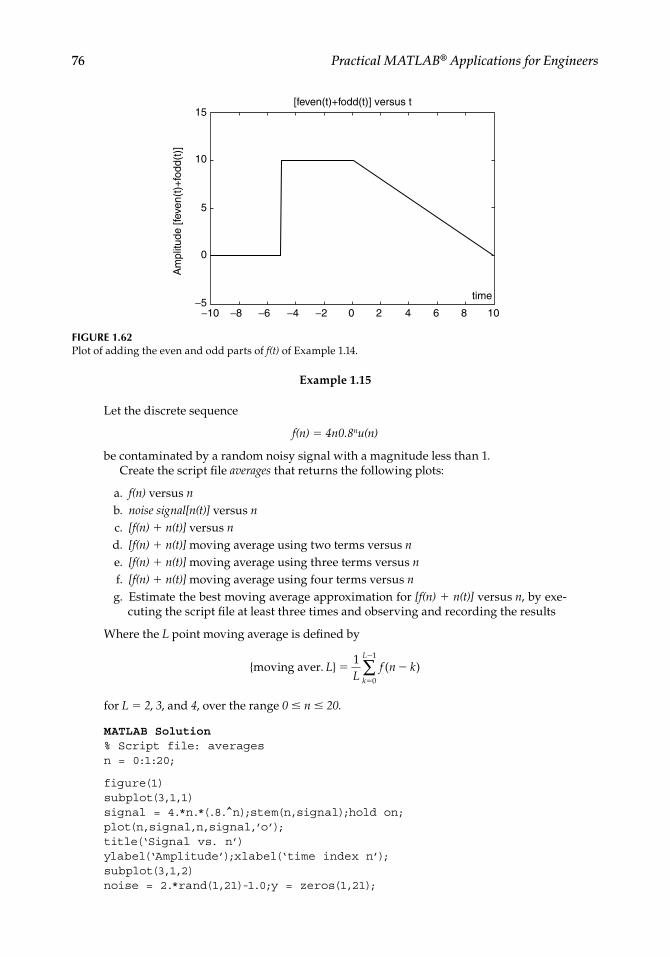
76 Practical MATLAB® Applications for Engineers
Example 1.15
Let the discrete sequence
f(n) = 4n0.8nu(n)
be contaminated by a random noisy signal with a magnitude less than 1.Create the script fi le averages that returns the following plots:
a. f(n) versus n b. noise signal[n(t)] versus n c. [f(n) + n(t)] versus n d. [f(n) + n(t)] moving average using two terms versus n e. [f(n) + n(t)] moving average using three terms versus n f. [f(n) + n(t)] moving average using four terms versus n g. Estimate the best moving average approximation for [f(n) + n(t)] versus n, by exe-
cuting the script fi le at least three times and observing and recording the results
Where the L point moving average is defi ned by
( )moving aver. L
Lf n k
k
L
1
0
1
∑
for L = 2, 3, and 4, over the range 0 ≤ n ≤ 20.
MATLAB Solution% Script file: averagesn = 0:1:20;
figure(1)subplot(3,1,1)signal = 4.*n.*(.8. n);stem(n,signal);hold on;plot(n,signal,n,signal,’o’);title(‘Signal vs. n’)ylabel(‘Amplitude’);xlabel(‘time index n’);subplot(3,1,2)noise = 2.*rand(1,21)-1.0;y = zeros(1,21);
FIGURE 1.62Plot of adding the even and odd parts of f(t) of Example 1.14.
[feven(t)+fodd(t)] versus t15
10
5
0
−5
Am
plitu
de [f
even
(t)+
fodd
(t)]
−10 −8 −6 −4 −2 0 2 4 6 8 10
time
CRC_47760_CH001.indd 76CRC_47760_CH001.indd 76 7/25/2008 4:16:25 PM7/25/2008 4:16:25 PM

Time Domain Representation of Continuous and Discrete Signals 77
plot(n,y);title(‘Noise vs. n’);hold on;stem(n,noise);hold on;plot(n,y,n,noise); ylabel(‘Amplitude’);xlabel(‘time index n’);axis([0 20 -1.3 1.3]);subplot(3,1,3);signoi =signal+noise;stem(n,signoi);title(‘[Signal + Noise] vs. n’);hold on;plot(n,signoi);ylabel(‘Amplitude[ signal+noise]’);xlabel(‘ time index n’)
figure(2)subplot(3,1,1)N = [.5 .5];D = 1;movave2 = filter(N,D,signoi);plot(n,signal,n,signoi,’s--’,n,movave2,’o-.’);legend(‘signal’,’signal+noise’,’moving ave/2term’)title(‘Various moving averages’);ylabel(‘magnitude’)subplot(3,1,2)N=[.33 .33 .33];D=1;movave3=filter(N,D,signoi);plot(n,signal,n,signoi,’s--’,n,movave3,’o-.’);ylabel(‘magnitude’)legend(‘signal’,’signal+noise’,’moving ave/3term’)subplot(3,1,3)N = [.25 .25 .25 .25];D = 1;movave4 = filter(N,D,signoi);plot(n,signal,n,signoi,’s--’,n,movave4,’o-.’);legend(‘signal’,’signal+noise’,’moving ave/4term’)ylabel(‘magnitude’);xlabel(‘ time index n’)
figure(3)plot(n,signal,n,signoi,’ks--’,n,movave2,’ko-.’);legend(‘signal’,’signal+noise’,’moving ave/2term’);title(‘Best approximation using moving averages’);ylabel(‘magnitude’);xlabel(‘ time index n’)
figure(4)err2 = signal-movave2;stem(n,err2);hold on;plot(n,y,n,err2);title(‘error=[mov.ave/2terms ] vs t’);ylabel(‘error’);xlabel(‘ time index n’)error1= sum(abs(signal-signoi)/21);error2 = sum(abs(signal-movave2)/21);error3 = sum(abs(signal-movave3)/21);error4 = sum(abs(signal-movave4)/21);disp(‘**************************************************’)disp(‘****************ANALYSIS OF ERROR****************’)disp(‘**************************************************’)disp(‘ no ave 2 term ave 3 term ave 4 term ave ‘);disp([error1 error2 error3 error4])disp(‘**************************************************’)disp(‘**************************************************’)
Back in the command window the script fi le averages is executed three times, and the results are shown as follows and in the plots of Figures 1.63 through 1.66.
CRC_47760_CH001.indd 77CRC_47760_CH001.indd 77 7/25/2008 4:16:26 PM7/25/2008 4:16:26 PM

78 Practical MATLAB® Applications for Engineers
FIGURE 1.63Plots of f(n), noise signal[n(t)], and [f(n) + n(t)] of Example 1.15.
Signal versus n10
5
0
1
0
0 2 4 6 8 10 12 14 16 18 20
−1
0 2 4 6 8 10 12 14 16 18 20
Am
plitu
deA
mpl
itude
Am
plitu
de [s
igna
l+no
ise]
time index n
time index n
time index n
Noise versus n
10
5
00 2 4 6 8 10 12 14 16 18 20
[Signal+Noise] versus n
>> averages
***************************************************************************ANALYSIS OF ERROR*************************************************************************** no ave 2 term ave 3 term ave 4 term ave 0.5389 0.5276 0.7011 0.9793****************************************************************************************************************
>> averages
***************************************************************************ANALYSIS OF ERROR********************************************************************* no ave 2 term ave 3 term ave 4 term ave 0.5272 0.4794 0.6574 0.9033****************************************************************************************************************
>> averages
***************************************************************************ANALYSIS OF ERROR********************************************************************* no ave 2 term ave 3 term ave 4 term ave 0.4144 0.3750 0.5572 0.8223****************************************************************************************************************
Observe that the results obtained by executing the script fi le averages three times are not the same, but in each case the best results are achieved when the moving average uses two terms.
CRC_47760_CH001.indd 78CRC_47760_CH001.indd 78 7/25/2008 4:16:26 PM7/25/2008 4:16:26 PM

Time Domain Representation of Continuous and Discrete Signals 79
Various moving averages10
5
0
signalsignal+noisemoving ave/2term
signalsignal+noisemoving ave/3term
signalsignal+noisemoving ave/4term
0 2 4 6 8 10 12 14 16 18 20
mag
nitu
dem
agni
tude
mag
nitu
de
10
10
5
5
00
00
2
2
4
4
6
6
8
8
10
10
12
12
14
14
16
16
18
18
20
20
time index n
FIGURE 1.64Plots of various moving averages of Example 1.15.
FIGURE 1.65Plots of f(n), [f(n) + n(t)], and best moving average of Example 1.15.
Best approximation using moving averages
signalsignal+noisemoving ave/2term
7
6
5
4
3
2
1
00 2 4 6 8 10 12 14 16 18 20
mag
nitu
de
time index n
CRC_47760_CH001.indd 79CRC_47760_CH001.indd 79 7/25/2008 4:16:26 PM7/25/2008 4:16:26 PM

80 Practical MATLAB® Applications for Engineers
Example 1.16
Let f(t) = te−1000t u(t)Create the script fi le sample_data that returns the following plots:
a. f(t) versus t, over the range 0 ≤ t ≤ 5 ms b. f(nT) versus nt, for T = 0.2 ms, over the range 1 ≤ n ≤ 26 c. Reconstruct f(t) from f(nT) using
i. Summations of sinc functions (emulating a low-pass fi lter) ii. Stair function iii. Spine function
d. error(t) versus t, for the reconstruction process when a low-pass fi lter is used, where
error t f t fn nT c F t nT F
Ts s Sn
N
SS
( ) ( ) ( )sin [ ( )] ,
1
26 1∑ for
MATLAB Solution% Script file: sample _ datat = 0:0.0005:0.005; % 26 time samplesfa = t.*exp(-1000.*t);
figure(1)subplot(2,1,1)plot(t,fa);title(‘f(t) vs t’)ylabel(‘Amplitude’);xlabel(‘time t (msec)’);subplot(2,1,2)Ts = 0.0002; n = 0:1:25; Fs=1/Ts;nTs = n*Ts;fd = nTs.*exp(-1000*nTs);stem(nTs,fd);hold on;plot(nTs,fd);title(‘f(t) sample with Ts=.2msec.’);ylabel(‘Amplitude’); xlabel(‘time index n (msec)’)
201816141210time index n
86420−1
−0.5
0
1
2
1.5
0.5
erro
r
error=[mov.ave/2terms] versus t
FIGURE 1.66Error plot of moving average using two terms of Example 1.15.
CRC_47760_CH001.indd 80CRC_47760_CH001.indd 80 7/25/2008 4:16:26 PM7/25/2008 4:16:26 PM

Time Domain Representation of Continuous and Discrete Signals 81
figure(2) % reconstructionsf25 = 0;for k = 1:1:26; fr25 = fd(k)*sinc(Fs*(t-k*Ts)); f25 = f25+fr25;endsubplot(3,1,1)plot(t,f25,’ko-’,t,fa,’ks-.’); legend(‘sinc-reconst’,’f(t)’);title(‘Reconstruction of f(t) ‘)ylabel(‘Amplitude’)subplot(3,1,2)stem(nTs,fd);hold on;stairs(nTs,fd); ylabel(‘Amplitude’);legend(‘stairs’)subplot(3,1,3)y = spline(nTs,fd,t);plot(nTs(1:2.5:26.5),y); legend(‘spline’);ylabel(‘Amplitude’)xlabel(‘time (sec)’)
figure(3)error=abs(fa-f25);plot(t,error);ylabel(‘magnitude’)title(‘error(t) = abs [f(t) - Reconstruction (Sums(sinc))]’)xlabel(‘time(sec)’)
Back in the command window the script fi le sample_data is executed and the results are shown in Figures 1.67 through 1.69.
FIGURE 1.67Plots of f(t) and f(nT) of Example 1.16.
0 0.5 1 1.5 2 2.5 3 3.5 4 4.5 5
× 10−3
× 10−4
× 10−4
time index n (msec)
0 0.5 1 1.5 2 2.5 3 3.5 4 4.5 5× 10⁻³
time t (msec)
4
2
0
Am
plitu
de
4
2
0
Am
plitu
de
f(t) versus t
f(t) sample with Ts=.2msec.
CRC_47760_CH001.indd 81CRC_47760_CH001.indd 81 7/25/2008 4:16:26 PM7/25/2008 4:16:26 PM

82 Practical MATLAB® Applications for Engineers
0 0.5 1 1.5 2 2.5 3 3.5 4 4.5 5
0 0.5 1 1.5 2 2.5 3 3.5 4 4.5 5
0 0.5 1 1.5 2 2.5 3 3.5 4 4.5 5
0
2
4
0
2
4
0
2
4
spline
stairs
f(t)
sinc-reconst
× 10−4
× 10−4
× 10−4
× 10−3
× 10−3
× 10−3
time (sec)
Reconstruction of f(t)
Am
plitu
deA
mpl
itude
Am
plitu
de
FIGURE 1.68Reconstruction plots for f(t) of Example 1.16.
8
7
6
5
4
3
2
1
1 1.5 2 2.50
0 0.5 3 3.5 4 4.5 5
time (sec) × 10−3
× 10−5 error(t) = abs [f(t) -Reconstruction (Sums(sinc))]
mag
nitu
de
FIGURE 1.69Reconstruction plot error for f(t) of Example 1.16.
CRC_47760_CH001.indd 82CRC_47760_CH001.indd 82 7/25/2008 4:16:27 PM7/25/2008 4:16:27 PM

Time Domain Representation of Continuous and Discrete Signals 83
Example 1.17
Create the script fi le up_down_samples that returns the approximation plots of the fol-lowing time discrete function:
f(n) = cos(2 0.05n) + 2 sin(20.03n)
for a length of N = 100 samples, for the following cases:
1. Down-sample or decimate the sequence f(n) with the integer factors of M = 2, 4, and 10.
2. Up-sample or interpolate the sequence f(n) with the integer factors of L = 2, 4, and 10.
3. Resample f(n) by the ratio of the two integers given by L/M, for the following cases: L = 3, M = 2, and L = 2, M = 3.
MATLAB Solution% Script file: up _ down _ samplesn = 0:1:99;f = cos(2*pi*.05*n)+2*sin(2*pi*.03*n);yzero = zeros(1,500);
figure(1); % down-sample with M=2, 4, 10subplot(2,2,1)stem(n,f);hold on; plot(n,f,n,yzero(1:100))title(‘f(n) vs n’); ylabel(‘Amplitude’);xlabel(‘time index n’);subplot(2,2,2)gm2 = decimate(f,2,’fir’);nm2 = 0:100/2-1;stem(nm2,gm2(1:50)); hold on; plot(nm2,yzero(1:50));title(‘f(n) is decimated with M=2’); ylabel(‘Amplitude’);xlabel(‘time index n’);subplot(2,2,3)gm4 = decimate(f,4,’fir’);nm4 = 0:100/4-1;stem(nm4,gm4(1:25));hold on;plot(nm4,gm4(1:25),nm4,yzero(1:25));ylabel(‘Amplitude’); xlabel(‘time index n’);title(‘f(n) is decimated with M=4’)subplot(2,2,4)gm10 = decimate(f,10,‘fir’);nm10=0:100/10-1;stem(nm10,gm10(1:10));hold on;plot(nm10,gm10(1:10),nm10,yzero(1:10));
CRC_47760_CH001.indd 83CRC_47760_CH001.indd 83 7/25/2008 4:16:27 PM7/25/2008 4:16:27 PM

84 Practical MATLAB® Applications for Engineers
ylabel(‘Amplitude’);xlabel(‘time index n’)title(‘f(n) is decimated with M=10’)
figure(2); % up-sample with L = 2, 4, 10subplot(2,2,1)stem(n,f); hold on; plot(n,f,n,yzero(1:100))title(‘f(n) vs n’);ylabel(‘Amplitude’);xlabel(‘time index n’);subplot(2,2,2)gL2 = interp(f,2);nL2 = 0:100*2-1;stem(nL2,gL2(1:200));hold on; plot(nL2,yzero(1:200));title(‘f(n) is upsampled with L=2’); ylabel(‘Amplitude’);xlabel(‘time index n’);subplot(2,2,3)gL4 = interp(f,4);nL4 = 0:100*4-1;stem(nL4,gL4(1:400)); hold on;plot (nL4,yzero(1:400));ylabel(‘Amplitude’);xlabel(‘time index n’);title(‘f(n) is upsampled with L=4’)subplot(2,2,4)gL10= interp(f,10);nL10 = 0:100*10-1;stem(nL10,gL10(1:1000));hold on;ylabel(‘Amplitude’); xlabel(‘time index n’)title(‘f(n) is upsampled with L=10’)
figure(3) % re-sample by ratio of L=3/M=2 & L=2/M=3subplot(3,1,1)stem(n,f);hold on; plot(n,f,n,yzero(1:100))title(‘f(n) vs n’);ylabel(‘Amplitude’); xlabel(‘time index n’);subplot(3,1,2)gr32= resample(f,3,2);nr32 = 0:100*3/2-1;yzeros = zeros(1,length(nr32));stem(nr32,gr32(1:100*3/2));hold on;plot(nr32,yzeros);ylabel(‘Amplitude’); xlabel(‘time index n’);subplot(3,1,3)gr23 = resample(f,2,3);nr23 = 0:100*2/3-1;yzero = zeros(1,length(nr23));stem(nr23,gr23(1:100*2/3));hold on;plot(nr23,yzero);axis([0 65 -5 5]);ylabel(‘Amplitude’); xlabel(‘time index n’)
Back in the command window, the script fi le up_down_samples is executed and the results are shown in Figures 1.70 through 1.72.
CRC_47760_CH001.indd 84CRC_47760_CH001.indd 84 7/25/2008 4:16:27 PM7/25/2008 4:16:27 PM

Time Domain Representation of Continuous and Discrete Signals 85
f(n) versus n f(n) is decimated with M=2
f(n) is decimated with M=4
4
2
0
−2
−4
4
2
0
−2
−4
Am
plitu
deA
mpl
itude
Am
plitu
de
time index n
0 50 100
4
2
0
0 10
−2
−4time index n
20 30
time index n
0 20 40 60
f(n) is decimated with M=104
2
0
−2
−4
Am
plitu
de
0 5 10
time index n
FIGURE 1.70Decimation plots of f(t) of Example 1.17.
f(n) versus n
f(n) is upsampled with L=4
4
0
−2
−4
2
Am
plitu
deA
mpl
itude
time index n
0 50 100
f(n) is upsampled with L=24
2
0
−2
−4
Am
plitu
de
0 50 100 150 200
time index n
f(n) is upsampled with L=104
2
0
−2
−4
Am
plitu
de
0 500
time index n
1000
4
2
−2
−4
0
0 100 200 300 400
time index n
FIGURE 1.71Interpolation plots of f(t) of Example 1.17.
CRC_47760_CH001.indd 85CRC_47760_CH001.indd 85 7/25/2008 4:16:27 PM7/25/2008 4:16:27 PM

86 Practical MATLAB® Applications for Engineers
Example 1.18
An analog communication system consists of an information signal or message given by m(t) = 3 cos(5t), and a high-frequency carrier given by fc(t) = cos(50t).
1. Create the script fi le modulation that returns the following plots: a. m(t) versus t b. fc(t) versus t c. Amplitude modulated (AM) signal versus t d. Angle modulated (FM/PM) signal versus t
2. Let us assume now that the message signal m(t) is a binary-periodic signal with period T = 2, defi ned as follows:
m t
t
t( )
3 0 1
1 1 2
Obtain the plots of the following communication signals:
a. ASK versus t b. FSK versus t c. PSK versus t
f(n) versus n5
−5
0
0
Am
plitu
deA
mpl
itude
Am
plitu
de
10 20 30 40 50 60 70 80 90 100
5
−5
0
f(n) is resampled with L=3/M=2
f(n) is resampled with L=2/M=3
0 50 100 150
time index n
time index n
5
0
0 10 20 30 40 50 60
time index n−5
FIGURE 1.72Plots of f(t) and resampled f(t) with notes given by L/M of Example 1.17.
CRC_47760_CH001.indd 86CRC_47760_CH001.indd 86 7/25/2008 4:16:28 PM7/25/2008 4:16:28 PM

Time Domain Representation of Continuous and Discrete Signals 87
MATLAB Solution% Script file: modulation
figure(1)subplot(2,2,1); % analog signalsfplot(‘3*cos(5*t)’,[0 3 -6 6]);title(‘Information signal: 3*cos(5*t)’);ylabel(‘Amplitude’);xlabel(‘time’);subplot(2,2,2)fplot(‘cos(50*t)’,[0 0.5 -1.5 1.5]);title(‘Carrier signal: cos(50*t)’);ylabel(‘Amplitude’);xlabel(‘time’);subplot(2,2,3)fplot(‘3*cos(50*t)*cos(5*t)’,[0 3 -6 6]);title(‘AM (Amplitude Modulated) signal’);ylabel(‘Amplitude’);xlabel(‘time’);subplot(2,2,4)fplot(‘3*cos((50*t)+3*cos(5*t))’,[0 2 -6 6]);title(‘Angle Modulated signal’);xlabel(‘time’);ylabel(‘Amplitude’);
figure(2)a=3*ones(1,50);b=ones(1,50);clock = [a b a b]; % discrete/binary signalst = linspace(0,4,200);carrier = cos(50*t);subplot(2,2,1)plot(t,clock);title(‘Binary information signal’);axis([0 4 0 4]);ylabel(‘Amplitude’);xlabel(‘time’);subplot(2,2,2)ASK= carrier.*clock;plot(t,ASK);title(‘ASK signal’)axis([0 4 -4 4]);ylabel(‘Amplitude’);xlabel(‘time’);subplot(2,2,3)FSK=cos(20*t.*clock);plot(t,FSK);xlabel(‘time’)axis([0 4 -1.3 1.3]);ylabel(‘Amplitude’)title(‘FSK signal’)subplot(2,2,4)PSK=cos(50*t+clock);plot(t,PSK);title(‘PSK signal’)xlabel(‘time’); ylabel(‘Amplitude’);axis([0 1.5 -1.3 1.3]);
Back in the command window the script fi le modulation is executed and the results are shown in Figures 1.73 and 1.74.
CRC_47760_CH001.indd 87CRC_47760_CH001.indd 87 7/25/2008 4:16:28 PM7/25/2008 4:16:28 PM

88 Practical MATLAB® Applications for Engineers
Binary information signal ASK signal4
3
2
1
0
Am
plitu
deA
mpl
itude
Am
plitu
deA
mpl
itude
0 1 2 3 4
time
4
2
−2
−4
0
0 1 2 3 4
time
PSK signal
1
0.5
−0.5
−1
0 0.5 1
0
1.5
time
FSK signal
1
0.5
−0.5
−1
0 1
0
2 3 4
time
FIGURE 1.74Plots of ASK, FSK, and PSK telecommunication signals for a binary information signal of Example 1.18.
Information signal: 3*cos(5*t)6
4
2
0
−2
−4
−6
Am
plitu
deA
mpl
itude
0 1 2 3
Am
plitu
deA
mpl
itude
Carrier signal: cos(50*t)1.5
1
0.5
0
−0.5
−1
−1.50
0 0.5 1 1.5 2
0.1 0.2 0.3 0.4
Angle Modulated signal
time
6
4
2
−2
−4
−6
0
time
time
AM (Amplitude Modulated) signal6
4
2
0
−2
−4
−60 1 2 3
time
FIGURE 1.73Plots of standard analog telecommunication signals of Example 1.18.
Example 1.19
Given the following time functions:
f1(t) = cos(2t) + 2 sin(3t)
and
f2(t) = 10 sin(2t)e−t/π over the range 0 ≤ t ≤ 2π.
CRC_47760_CH001.indd 88CRC_47760_CH001.indd 88 7/25/2008 4:16:28 PM7/25/2008 4:16:28 PM

Time Domain Representation of Continuous and Discrete Signals 89
Create the script fi le multiplex that returns the following plots:
a. f1(t) and f2(t) are sampled with a sampling rate of Ts = 2π/100. b. The multiplex signals of part a.
MATLAB Solutiont = linspace(0,2*pi,100);f1 = cos(2*t)+2*sin(3*t);f2 = 10*sin(2*t).*exp(-t/pi);yzero = zeros(1,100);
figure(1)subplot(2,2,1)plot(t,f1,’dk’,t,f2,’sk’,t,yzero);axis([0 2*pi -6 10])legend(‘f1(t)’,’f2(t)’)title(‘f1(t) vs. n and f2(t) vs. t’)ylabel(‘Amplitude’); xlabel(‘time index n’)subplot(2,2,2)a = [1 0 1 0 1 0 1 0 1 0];aa = [a a a a a a a a a a];b = [0 1 0 1 0 1 0 1 0 1];bb = [b b b b b b b b b b];f1samp = f1.*aa;f2samp = f2.*bb;stem(t(1:2:100),f1(1:2:100));hold on; plot(t,yzero);title(‘f1(n) vs. n’)axis([0 2*pi -4 5]);ylabel(‘Amplitude’);xlabel (‘time index n’);subplot(2,2,3)stem(t(1:2:100),f2(1:2:100));hold on;plot(t,yzero)title(‘f2(n)vs. n’)axis([0 2*pi -6 10]);ylabel(‘Amplitude’)xlabel(‘time index n’)subplot(2,2,4);stem(t(1:2:100),f1(1:2:100),‘d’);hold on;stem(t(1:2:100),f2(1:2:100),‘s’);hold on; plot(t,yzero);axis([0 2*pi -6 10]);title(‘ [Multiplexed samples of f1(n) and f2(n)] vs. n’);legend(‘f1(t)’,‘f2(t)’)xlabel(‘time index n’)
figure(2)plot(t(1:2:50),f1(1:2:50),t(1:2:50),f2(1:2:50),t,yzero);hold on; stem(t(1:2:50),f1(1:2:50),‘d’); hold on;stem(t(2:2:50),f2(2:2:50),‘s’);title(‘ [Enlarge alternating (multiplexed) samples from f1(n)
and f2(n)] vs. n ‘)axis([0 3.1 -6 10]);ylabel(‘Amplitude’);xlabel(‘time index n’)
Back in the command window the script fi le multiplex is executed and the results are shown in Figures 1.75 and 1.76.
CRC_47760_CH001.indd 89CRC_47760_CH001.indd 89 7/25/2008 4:16:28 PM7/25/2008 4:16:28 PM

90 Practical MATLAB® Applications for Engineers
10
5
0
0 2 4 6
0 2 4 6
0 2 4 6
0 2 4 6
−5
4
2
0
−4
−2
time index n
time index n time index n
time index n
f1(t)
f1(t) versus n and f2(t) versus n
f2(t)
f1(t)
f2(t)
f1(n) versus n
f2(n) versus n [Multiplexed samples of f1(n) and f2(n) versus n]
Am
plitu
de
10
5
0
−5
Am
plitu
de
Am
plitu
de
10
5
0
−5
Am
plitu
de
FIGURE 1.75Plots of discrete telecommunication signals of Example 1.19.
10
8
6
4
2
0
0 0.5 1 1.5time index n
Am
plitu
de
2 2.5 3
−2
−4
−6
[Enlarge alternating (multiplexed) samples from f1(n) and f2(n)] versus n
FIGURE 1.76Enlarge plot of multiplexed signals of Example 1.19.
CRC_47760_CH001.indd 90CRC_47760_CH001.indd 90 7/25/2008 4:16:28 PM7/25/2008 4:16:28 PM

Time Domain Representation of Continuous and Discrete Signals 91
Example 1.20
Create the script fi le explore_window that returns the plots of the truncated or windowed function f(t) = cos(2πt) using the following window types:
1. Hamming 2. Hanning 3. Blackman 4. Kaiser (with β = 3.4) 5. Triangular 6. Boxcar 7. Bartlett
Let us defi ne f(t) = cos(2πt) by using 301 points over the range −15 ≤ t ≤ 15, and limit f(t) using the above-mentioned windows over the range −10 ≤ t ≤ 10.
Display the plots of the windowed function f(t) over the range −15 ≤ t ≤ 15, for the fi rst three cases and −10 ≤ t ≤ 10, for the remaining four.
MATLAB Solution% Script file: explore _ windowt = -15:0.1:15; % returns a vector with 301 elementsf = cos(2*pi*t); % returns 301 element for f(t)winpoints = -100:1:100; % 201 window pointsWHam=hamming(201);WHan= hanning(201);WBlac= blackman(201);WKai= kaiser(201, 3.4); % Beta = 3.4WTrian= triang(201);WRect= boxcar(201);WBar= bartlett(201);W1Ham= [zeros(1,50) WHam’ zeros(1,50)]; % Hamming window with 301
pointsW1Han = [zeros(1,50) WHan’ zeros(1,50)]; % Hanning window with 301
pointsW1Blac = [zeros(1,50) WBlac’ zeros(1,50)]; % Blackman window with 301
pointsW1Kai = [ zeros(1,50) WKai’ zeros(1,50)] ; % Kaiser window with 301
pointsW1Tria = [ zeros(1,50) WTrian’ zeros(1,50)]; % Triangular window with
301 pointsW1Box = [ zeros(1,50) WRect’ zeros(1,50)]; % Boxcar window with 301
pointsW1Bar = [ zeros(1,50) WBar’ zeros(1,50)] ; % Bartlett window with 301
pointsHamwin= W1Ham.*f; % f(t) is windowedHanwin= W1Han.*f;Blackwin =W1Blac.*f;Kaiwin=W1Kai.*f;Triwin=W1Tria.*f;Boxwin=W1Box.*f;Barwin=W1Bar.*f;
figure(1)subplot(3,1,1)plot(t, Hamwin);ylabel(‘Amplitude’);title(‘[f(t)*Hamming widow] vs.t’)
CRC_47760_CH001.indd 91CRC_47760_CH001.indd 91 7/25/2008 4:16:29 PM7/25/2008 4:16:29 PM

92 Practical MATLAB® Applications for Engineers
axis([-15 15 -1.2 1.2]);subplot(3,1,2);plot(t, Hanwin);axis([-15 15 -1.2 1.2]);ylabel(‘Amplitude’);title(‘ [f(t)*Hanning widow] vs. t’);subplot(3,1,3);plot(t, Blackwin);axis([-15 15 -1.2 1.2]);xlabel(‘t’);title(‘[f(t)*Blackman widow] vs.t’)ylabel(‘Amplitude’)
figure(2)subplot(2,2,1)plot(t, Kaiwin);ylabel(‘Amplitude’)title(‘[f(t)*Kaiser window] vs. t’)axis([-10 10 -1.2 1.2]);subplot(2,2,2)plot(t,Triwin );ylabel(‘Amplitude’);title(‘[f(t)*Triang. window] vs. t’);axis([-11 11 -1.2 1.2]);subplot(2,2,3)plot(t,Boxwin );ylabel(‘Amplitude’);title(‘[f(t)*Boxcar window] vs. t’);axis([-11 11 -1.2 1.2]);xlabel(‘t’)subplot(2,2,4)plot(t,Barwin );ylabel(‘Amplitude’)title(‘[f(t)*Barlett window] vs. t’)axis([-11 11 -1.2 1.2]);xlabel(‘t’)
Back in the command window, the script fi le explore_window is executed and the results are shown in Figures 1.77 and 1.78.
1
0
−1
−15 −10 −5 0 5 10 15
t
1
0
−1
−15 −10 −5 0 5 10 15
t
1
0
−1
−15 −10 −5 0 5 10 15
t
[f(t)*Hamming window] versus t
[f(t)*Hanning window] versus t
[f(t)*Blackman window] versus t
Am
plitu
deA
mpl
itude
Am
plitu
de
FIGURE 1.77Plots of the windowed function f(t) using the Hamming, Hanning, and Blackman windows of Example 1.20.
CRC_47760_CH001.indd 92CRC_47760_CH001.indd 92 7/25/2008 4:16:29 PM7/25/2008 4:16:29 PM

Time Domain Representation of Continuous and Discrete Signals 93
1.5 Application Problems
P.1.1 Sketch by hand, over the range −3 ≤ t ≤ 6, the following analog functions: a. ƒ1(t) = 5u(t − 2)
b. ƒ2(t) = 3u(t − 1) − 3u(t − 3)
c. ƒ3(t) = t[u(t − 1) − u(t − 2)]
d. ƒ4(t) = δ(t + 1) + 2δ(t − 1) + u(t − 2)
e. ƒ5(t) = t[u(−t) * u(t + 3)]
f. ƒ6(t) = u(t + 1) − u(t) + 3δ(t − 3)
P.1.2 Sketch by hand, over the range −3 ≤ n ≤ 6, the following discrete sequences: a. ƒ1(n) = 3(n − 2)u(n)
b. ƒ2(n) = n u(n)
c. ƒ3(n) = (−n)2 u(n)
d. ƒ4(n) = −3δ(n + 2) + 2δ(n) + u(n) + u(n − 1) + 2u(n − 1)
e. ƒ5(n) = 2η[u(n) − u(n − 2)]
f. ƒ6(n) = n[u(n + 2) . u(−n)]
1
0.5
−0.5
−1
−10 −5
0
0 5 10
1
0.5
−0.5
−1
−10 −5
0
1
0.5
−0.5
−1
0
0 5 10 −10 −5 0 5 10
1
0.5
−0.5
−1
−10 −5
0
0 5 10
[f(t)*Kaiser window] versus t
[f(t)*Boxcar window] versus t
[f(t)*Triang. window] versus t
[f(t)*Barlett. window] versus t
t t
tt
Am
plitu
deA
mpl
itude
Am
plitu
deA
mpl
itude
FIGURE 1.78Plots of the windowed function f(t) using the Kaiser, Triangular, Boxcar, and Bartlett windows of Example 1.20.
CRC_47760_CH001.indd 93CRC_47760_CH001.indd 93 7/25/2008 4:16:30 PM7/25/2008 4:16:30 PM

94 Practical MATLAB® Applications for Engineers
P.1.3 Create a script fi le that returns the plots of each of the functions defi ned in P.1.1.P.1.4 Create a script fi le that returns the plots of each of the sequence defi ned in P.1.2.P.1.5 Sketch by hand, over the range −1 ≤ n ≤ 8, the sequence ƒ(n) = (0.32)n [u(n) −
u(n − 6)].
P.1.6 Let ƒ(n) = (0.32)n [u(n) − u(n − 6)], over −1 ≤ n ≤ 8.Write a script fi le that returns the following plots:
a. ƒ(n) versus n
b. ƒ(2n) versus n
c. ƒ(n/2) versus n
d. ƒ(n − 3) versus n
P.1.7 Given the sequence f n n mm
m( ) ( / ) ( )
1 20
∑a. Write a program that returns the plot of ƒ(n) versus n, over the range 0 ≤ n ≤ 30.b. Evaluate the energy and power of f(n).
P.1.8 Given the sequence ƒ(n) = 15(0.75)n u(n). Create the script fi le that returns the plot of ƒ(n) versus n, over the range −10 ≤ n ≤ 30.
Observe and discuss if the sequence f(n) diverges or converges.P.1.9 Given the sequence ƒ(n) = 0.2(1.1)n u(n), create a script fi le that returns the plots of
ƒ(n) versus n, over the range −10 ≤ n ≤ 30.Discuss if the sequence f(n) converges or diverges.
P.1.10 Given the following analog signals:
1. ƒ1(t) = 4e−2t u(t)
2. ƒ2(t) = 5e−1.5t cost(5t − π/2)u(t)
3. ƒ3(t) = 6(1 − e−2t)u(t)
4. ƒ4(t) = e−tcos(5t − π/4)u(t)
(a) Sketch by hand each of the given functions versus t. (b) Write a program that returns the plots of each of the functions of part (a), over the range −1 < t < 6.
P.1.11 Write a MATLAB program that returns the plots of the continuous function ƒ(t) = 3 cos(0.15πt) + 2sin(0.20πt), and f(t) sampled with TS = 0.1π over the range 0 < t < 15π.
P.1.12 In general, a random noisy signal of length N can be generated by using the follow-ing MATLAB command:
Noise=rand(1,N)
Likewise, the sequence
Noisen=randn(1,N)
returns a random sequence of length N, normally distributed with zero mean and unit variance. Write a program that returns the plots, the average value, the maxima, and minima of each of the noisy sequences defi ned earlier for N = 100 and 200.
CRC_47760_CH001.indd 94CRC_47760_CH001.indd 94 7/25/2008 4:16:30 PM7/25/2008 4:16:30 PM

Time Domain Representation of Continuous and Discrete Signals 95
P.1.13 Plot the functions indicated as follows over the range −3 ≤ t ≤ 3:
f1(t) = t3
f2(t) = 3 + t3
f3(t) = 2t3 + t5 + 3
f4(t) = tan(2t)
f5(t) = sin(2t)
and verify that all the preceding functions present odd symmetry, that is, f(t) = −f(t).
P.1.14 Plot the functions indicated as follows for the range −3 ≤ t ≤ 3:
f1(t) = t2
f2(t) = 3 + t2
f3(t) = 2t4 + t6 + 3
f4(t) = cos(2t)
f5(t) = |t|
and verify that all the preceding functions present even symmetry, that is, f(t) = f(−t).P.1.15 Write a MATLAB function fi le that analyzes a given arbitrary function f(t) over the
range −3 ≤ t ≤ 3, and returns a message indicating if f(t) presents even or odd sym-metry. Repeat the preceding problem over any given range.
P.1.16 Given the functions shown in Figure 1.79, sketch by hand for each function its even and odd parts.
f1(t )
f4(t )
f2(t) f3(t )
f5(t )
f7(t )f6(t )
tt
t t
−1 0
−1
+1−1
1
2
2
0 0 2 −2 2
t t t1
33
2
1 0
−1 0 3 −1 0 3
1
1
2
1 2
FIGURE 1.79Plots of P.1.16.
CRC_47760_CH001.indd 95CRC_47760_CH001.indd 95 7/25/2008 4:16:30 PM7/25/2008 4:16:30 PM

96 Practical MATLAB® Applications for Engineers
P.1.17 Write a program that returns the plots over three cycles of the following periodic functions, defi ned as follows over one period (T = 2):
ƒ1(t) = t, for 0 < t <2
ƒ2(t) = −t + 2, for 0 < t < 2
f t
t
t3
2 0 1
0 1 2( )
f n
t
t4
1 0 1
2 1 2( )
ƒ5(t) = 2 + t, 0 < t < 2
ƒ6(t) = −t + 4, 0 < t < 2
P.1.18 Sketch by hand each of the functions defi ned in P.1.13.P.1.19 Sketch by hand the even and odd portions of each of the functions defi ned in P.1.13.P.1.20 Let f(t) be a periodic function with period T = 2, defi ned as follows by
f t
t t
t( )
0 1
1 1 2
a. Manually sketch f(t) over three periodsb. Write a program that returns the plots of part ac. Sketch by hand f(−t)d. Write a program that returns the plot of part ce. Sketch by hand [f1(t) = −f(−t) + f(t)] versus t, over the range −3 ≤ t ≤ +3f. Write a program that returns the plot of part eg. Sketch f2(t) = 1 _ 2 [f(t) + f(−t)] versus t and f3(t) = 1 _ 2 [f(t) − f(−t)] versus t, over the
range −3 ≤ t ≤ +3h. Sketch by hand [f4(t) = f2(t) + f3(t)] versus t
P.1.21 Modify the script fi le even_odd.m (of Example 1.14) into a function fi le where the input is the function f(t), over a given range r, and its outputs are the plots of the even and odd parts of f(t).
P.1.22 Test the function fi le even_odd.m created in P.1.21, over the range −10 ≤ t ≤ 10, using the following function:a. f1(t) = cos(3t + pi/3)u(t)
b. f2(t) = t u(t)
c. f3(t) = t u(t) − t u(t − 5)
P.1.23 Let f(t) = 3r(t) − 3r(t − 1) + 3r(t − 2), sketch and obtain MATLAB plots, over the range −5 ≤ t ≤ 5, for the following functions:a. f(t) versus t
b. fe(t) versus t
c. fo(t) versus t
CRC_47760_CH001.indd 96CRC_47760_CH001.indd 96 7/25/2008 4:16:31 PM7/25/2008 4:16:31 PM

Time Domain Representation of Continuous and Discrete Signals 97
P.1.24 Let f1(t) = 3e2t/3 + 3 and f2(t) = cos(πt). Create a script fi le that returns the energy and power of f1(t) and f2(t).
P.1.25 Repeat P.1.24 for the following discrete sequences: f1(n) = 3e2n/3 + 3 and f2(n) = cos(0.1πn), over the range −10 ≤ n ≤ 10.
P.1.26 Evaluate by hand which of the following discrete sequences are periodic, and if periodic, evaluate its period.a. cos(0.2n)
b. cos(0.2πn)
c. sin(2πn/3)
d. sin(9.1n)
P.1.27 Verify the following equalities:
a. Imp[( )]n
( )n kk∑
b. u n[( )]
( )n kk 0∑
c. r n k n kk
( ) ( )
0
∑P.1.28 Evaluate the following integrals:
a. ( ) ( )2 3 1t t dt+∫
b. ( ) (( / ) )2 3 3 2 1t t dt+∫
c. sin( ) (( / ) ( / ))wt t dt 3 2 2 3
∫d. e t dtt( ) ( ( / ))
3 1 1 2 3∫
P.1.29 Analyze and draw a fl ow chart of Example 1.15 and indicate in each average approx-imation the fi lter used as well as the effect of the fi lter.
P.1.30 Evaluate the fi rst and second derivative of the following expressions:a. f1(t) = u(t) + 7u(t − 5) − 2u(t − 7)
b. f2(t) = tu(t) + e3tu(t − 1) + 3δ(t − 3)
c. f3(t) = r(t)u(t) − r(t − 1)u(t − 1)
P.1.31 Let H(s) = s + 3 _______________ s3 + s2 + 5s + 10
be the transfer function of a given analog system. Write
a MATLAB program that returns a. The Bode plot of H(s), magnitude and phaseb. The impulse as well as the step responsesc. The zero/pole diagramd. The system differential equation
P.1.32 Let
H z
z z zz z z
( ). . . .
. . .
0 32 0 43 0 85 0 21 0 802 0 42 0 62
1 2 3
1 2 3
−
− − −
CRC_47760_CH001.indd 97CRC_47760_CH001.indd 97 7/25/2008 4:16:31 PM7/25/2008 4:16:31 PM

98 Practical MATLAB® Applications for Engineers
be the transfer function of a discrete system. Write a MATLAB program that returnsa. The impulse as well as the step responseb. The zero/pole diagramc. The system output if its input is given by
x(n) = 0.6ncos((2 * pi * n)/(256)), for n = 0, 1, 2, 3, …, 256
d. The plot of the output if the input x(n) given in part c is truncated by a triangular window with size of N = 128
e. Repeat part d for the Hamming, Hanning, and Blackman windowsP.1.33 Write a program (or programs) that returns the sequences and plots shown in Fig-
ure 1.80.P.1.34 The Parabolic or Parzen window is defi ned by the following equation:
w n
n MM
( )
12
Write a program that returns the plots of w(n) versus n, for n = 31 and M = 0.5, 1, and 5, and discuss the effect of M.
y1(x)
y3(x)
y5(x) y6(x)
y4(x)
y2(x)
2
−10 −1
−2 −1
−4−3 −1 1
2
3 10−2
1
1
2
2
2
4
2
0 2
1
3
0 0
0
0 0
10
2 4
1 10 −10 −1 1
12
3
10x
x
x
x
x
1
1
x
FIGURE 1.80Plots of P.1.33.
CRC_47760_CH001.indd 98CRC_47760_CH001.indd 98 7/25/2008 4:16:31 PM7/25/2008 4:16:31 PM

Time Domain Representation of Continuous and Discrete Signals 99
P.1.35 The Cauchy window is defi ned by the following equation:
w n
MM n M
( )( )
2
2 2 2
Write a program that returns the plots of w(n) versus n, for n = 31 and α = 0.5, 1, 3, and 5, and discuss the effect of α.
P.1.36 The Gaussian window is defi ned by the following equation:
w n
n MM
( ) exp .
0 5 22
Write a program that returns the plots of w(n) versus n, for n = 31, M = 0.5, and α = 1, 3, and 5, and discuss the effect of α.
P.1.37 Consider the following discrete time sequences:
f n
nn1
20 3 64
0 3 64( )
sin[ . ( )]. ( )
f n
nn2
20 2 64
0 2 64( )
sin[ . ( )]. ( )
Write a program that returnsa. The plots of f1(n) versus n and f2(n) versus n, over 0 ≤ n ≤ 128 using the sinc func-
tion, and appropriately label the axis.b. The plots of the expanded signals f1(n) and f2(n) by a factor L, by inserting L − 1
zeros between each one of the samples of f1(n) and f2(n), for L = 2, 3, and 4. There-fore, each signal f1(n) and f2(n) is expanded by a factor of 2, 3, and 4.
c. The plots of the down-sampled signals f1(n) and f2(n) by a factor of M = 2, 3, and 4.P.1.38 Truncate or limit the length of each of the functions f1(n) and f2(n) defi ned in P.1.37
by using the following windows:a. Parabolicb. Cauchyc. Gaussian
defi ned in P.1.34/36 over a length of N = 31.P.1.39 Obtain the multiplex signal mult[f1(n), f2(n)]; for the sequences f1(n) and f2(n) given by
f n
nn1
20 3 64
0 3 64( )
sin[ . ( )]. ( )
f n
nn2
20 2 64
0 2 64( )
sin[ . ( )]. ( )
P.1.40 Consider the analog time functions
f1(t) = [5sin(3πt)/(3πt)]2
f2(t) = [3sin(2πt)/(2πt)]2
CRC_47760_CH001.indd 99CRC_47760_CH001.indd 99 7/25/2008 4:16:31 PM7/25/2008 4:16:31 PM

100 Practical MATLAB® Applications for Engineers
Write a program that returnsa. The plots of f1(t) versus t and f2(t) versus t, over the range −2π ≤ t ≤ 2π, using the
sinc functionb. The plots of the amplitude modulated (AM) signals for f1(t) and f2(t) versus t,
over the range 0 ≤ t ≤ 3, if the carrier signal is fc(t) = 10 cos(20πt)
c. Repeat part b for the case of angular modulation (FM or PM)P.1.41 Let f(t) = A cos(2πwot + φ) be a continuous time function.
How many samples are then required to uniquely determine A, wo, and φ.Is it always possible to solve for A, wo, and φ?
P.1.42 Let A = 5, wo = 2 rad/s, and φ = 30°, for the signal defi ned in P.1.41.Write a program that returns the following plots:
a. f(t) versus t
b. f(nT) versus nT, for T = 0.1
c. Reconstruct f(t) from f(nT) using the summation of sinc functions (by applying the sampling theorem)
P.1.43 Create the symbolic expression for f(t) defi ned in P.1.42 and obtain the following plots:a. f(t) versus t, using ezplot.b. Let A = 7, wo = 3 rad/s, and φ = 45° by redefi ning the symbolic expression of
part a, by using the subs symbolic function.c. AM and FM/PM signals using the symbolic approach, if the carrier is fc(t) =
10 cos(20πt) and the information is f(t).
CRC_47760_CH001.indd 100CRC_47760_CH001.indd 100 7/25/2008 4:16:31 PM7/25/2008 4:16:31 PM

101
2Direct Current and Transient Analysis
I often say that when you can measure what you are speaking about, and express it in numbers, you know something about it; but when you cannot express it in numbers, your knowledge is of meager and unsatisfactory kind.
Lord Kelvin
2.1 Introduction
This chapter deals with the basic concepts and principles of electricity as well as the analysis of simple electric circuits. A brief and compressed history of electricity is also presented to introduce the reader to how this important fi eld of science and engineering evolved over time.
The simplest manifestation of electricity in nature is the phenomenon of magnetism and static electricity. Static electricity was fi rst observed by the ancient Greeks, and back then they called this phenomenon elektron. The curious Greeks observed and studied the effects of elektron, but no written records about the subject exist.
The fi rst recorded observations about electricity and magnetism date back to Thales (640–546 BC), a famous philosopher and mathematician who lived on the west coast of Asia Minor. Years later, the Chinese military commanders, during the Hun dynasty (AD 206–220) are believed to have used the magnet’s properties to implement the fi rst compass to indicate direction. It took about 900 years for the Europeans to incorporate the compass in navigation. No signifi cant recorded scientifi c progress was made in electric-ity and magnetism until the 1600s, when William Gilbert (1540–1603), Queen Elizabeth’s physician, recorded experiments he performed with magnetic materials. He thought that magnetism could have healing effects on the human body.
Probably the fi rst major modern scientifi c contribution was the Leyden jar developed by Pieter van Musschenbrock and Benjamin Franklin. The jar was a device capable of storing an electric charge (static electricity), which could be discharged producing an electric arc or spark, thus emulating lighting.
Years later, it was discovered that lightning was in essence an electric discharge. The most important scientifi c contributions occurred during the late 1700s through the late 1800s, when the effects of electricity and magnetism were observed, recorded, and seri-ously studied. Concepts and principles once understood, tested, and proven became rules, laws, and theories.
A number of electric units bear the name of those early pioneers, such as
Coulomb. After Charles Coulomb (1736–1806), Frenchman; observed, measured, and quantized the amount of electricity (electric charge)Ampere. After Andres Maria Ampere (1775–1836), Frenchman; studied the current induced by a magnetic fi eld
•
•
CRC_47760_CH002.indd 101CRC_47760_CH002.indd 101 7/23/2008 1:38:32 PM7/23/2008 1:38:32 PM

102 Practical MATLAB® Applications for Engineers
Volt. After Count Alexander Volta (1747–1827), Italian; developed the voltaic cellOhm. After Georg Ohm (1787–1854), German; developed a relationship among the current, voltage, and resistance in an electric circuitFaraday. After Michael Faraday (1791–1867), Englishman; developed the basis of the electromagnetic theoryHertz. After Heinrich Rudolph Hertz (1857–1894), German; experimented with elec-tromagnetic waves
Two additional names are associated with the early developments of electric theories and discoveries, and their work constitutes the basis of electric circuits. They are:
James Clark Maxwell (1831–1879), Scottish. Maxwell developed the relationship between electricity and magnetism, as well as the electromagnetic theory of light (1862).
Gustav Robert Kirchhoff (1824–1887), Russian. Kirchhoff formulated the basic circuit laws (the network current and voltage laws).
The theoretical fundamentals of electricity and magnetism were observed, studied, and fi rmly established, predominantly by European physicists, engineers, and mathematicians.
American scientists and engineers are distinguished as the great inventors, patent hold-ers, and industrialists who brought the electric discoveries into the market place. The most important Americans, just to mention a few, are
Thomas Edison (1847–1931)Alexander Graham Bell (1847–1922)Lee De Forest (1873–1961)
Today we know that electricity is produced by electrons. An electron is the smallest unit of electric charge, and its quantity is known as “1 esu.” An electron is not easily found in nature, but it can be generated, and it constitutes the most important source of energy in modern societies. In its simplest version, the concepts of current and voltage constitute the bases of electricity.
Let us defi ne current and voltage using the simplest possible terms. Current is the fl ow (movement) of electrons, whereas voltage is the force that makes this fl ow possible.
This chapter deals with DC electrical systems and transients. The term “DC” is an abbre-viation of direct current, which refers to electrical sources that employ unidirectional cur-rent. These sources of voltage or current provide a fi xed or constant output.
A current that varies with respect to time reversing directions periodically is called alternating current, abbreviated as “AC,” and is the subject of Chapter 3.
DC voltage sources consist of batteries, generators, and power supplies. These devices employ different technologies and modes of operations, but the end result is to supply a constant terminal voltage, regardless of the current demand and load connected to its terminals.
A DC current source is analogous to a voltage source in the sense that it supplies a con-stant current fl ow, whereas the voltage demand may vary across its terminals.
DC is produced either by a voltage or current source that delivers a constant output, denoted mathematically as e(t) = E V (volts) or i(t) = I A (amp) respectively, and the electrical responses (steady state) in any of its branches of an electrical network are also constant.
•
•
•
•
•••
CRC_47760_CH002.indd 102CRC_47760_CH002.indd 102 7/23/2008 1:38:34 PM7/23/2008 1:38:34 PM

Direct Current and Transient Analysis 103
When a circuit switches from one condition to a new set of conditions, there is a transi-tion period where the currents and voltages adjust to the new circuit conditions. The tran-sition time is referred to as the transient response or simply as transient, and is usually defi ned by a set of differential equations.
The basic passive circuit elements such as resistors, capacitors, and inductors are intro-duced, defi ned, and used in this chapter. Circuit variables such as voltage, current, power, and energy are also defi ned in terms of the circuit elements and its excitations; and transient conditions for the standard electrical confi gurations are stated, explored, and analyzed.
2.2 Objectives
On reading this chapter, the reader should be able to
Distinguish between DC and ACState the laws of attraction and repulsion (Coulomb’s law) at the subatomic levelDefi ne ampere (the unit of electric current) and volt (the unit of electric voltage) quantitatively and qualitativelyRelate current, charge, and timeDefi ne the concept of conductor, superconductor, semiconductor, and insulatorDefi ne and know Ohm’s lawDefi ne an electrical short and open and its electrical equivalentsDefi ne and know how to use the basic electric concepts and terminology such as voltage drop, current fl ow, and resistanceRecognize a series and parallel connectionDraw schematic diagrams of simple electric circuitsState Kirchhoff’s current law (KCL) and Kirchhoff’s voltage law (KVL)State the voltage divider ruleState the current divider ruleKnow how and when to apply the voltage or current divider rulesDefi ne electric power and energyState the equations that defi ne the energy storing devices such as the inductor (L) and capacitor (C)Combine resistors, capacitors, and inductors in a series and parallel confi gurationCalculate the equivalent capacitance and inductanceState the conditions for the steady-state and transient responsesDefi ne the time constant of an electric circuit and its meaning and applicationsPresent the equation and plots of the charging and discharging for the simple circuits known as resistor capacitor (RC) and resistor inductor network (RL)Set up the circuit equations for simple circuitsState the differential equations and the exponential form of the solution for the RC and RL cases
•••
•••••
••••••••
•••••
••
CRC_47760_CH002.indd 103CRC_47760_CH002.indd 103 7/23/2008 1:38:34 PM7/23/2008 1:38:34 PM

104 Practical MATLAB® Applications for Engineers
State and analyze the transient solution for the parallel and series resistor capacitor network (RLC)Defi ne the system loop and node equationsUse node and loop equations to solve circuit problemsDefi ne and use the superposition theorem when dealing with multiple sourcesRecognize that an independent voltage source set to zero is equivalent to a short circuitRecognize that an independent current source set to zero is equivalent to an open circuitRecognize that a voltage source can be transformed into an equivalent current source and vice versaDefi ne and determine the Thevenin’s equivalent circuit of an electrical networkRecognize that the Thevenin’s equivalent circuit can be evaluated for any load of interestDefi ne and determine the Norton’s equivalent circuit given an electrical networkRecognize that the relation between Thevenin’s and Norton’s equivalent circuits consist of a simple source transformationUse MATLAB® as a tool in the analysis of electric circuits
2.3 Background
R.2.1 The idea that matter is composed of atoms is an old concept that was fi rst proposed by the Greek philosophers Empedocles and Democritus around 500 and 400 BC.
R.2.2 The scientifi c community accepted the existence of the atom in modern times, ini-tially proposed by the chemist Dalton in the nineteenth century, and supported and consolidated by Cannizzaro 50 years later.
R.2.3 An atom is too small to be seen directly or even with the help of modern and sophis-ticated devices such as a microscope, because its diameter is estimated to be in the order of 10−10 m.
R.2.4 Atoms are composed of protons, neutrons, and electrons.R.2.5 In modern times, J. J. Thomson, around 1897, is credited with the discovery and
study of the electron.R.2.6 The mass of a neutron is slightly larger than the mass of a proton, and the mass of
an electron is much smaller than either of them.R.2.7 An electron constitutes the unit of a negative electric charge.R.2.8 A proton constitutes the unit of a positive electric charge.R.2.9 Atoms move in nature in a perfectly random way.R.2.10 The effect of an electron exactly cancels the effect of a proton.R.2.11 An atom contains a certain number of protons in a nucleus and an equal number of
electrons orbiting the nucleus.R.2.12 Most bodies in nature are electrically neutral, because they contain equal amounts
of positive and negative charges that exactly cancel one another.
•
••••
•
•
••
••
•
CRC_47760_CH002.indd 104CRC_47760_CH002.indd 104 7/23/2008 1:38:34 PM7/23/2008 1:38:34 PM

Direct Current and Transient Analysis 105
R.2.13 By a process that is known to scientists, but is beyond the scope of this discussion, energy may be absorbed by some electrons in the outer orbits and migrate outside its natural orbits, and in this way, become free electrons.
R.2.14 In metals such as silver and copper, some electrons are very loosely held, since they are not strongly attached to any atom, and they can be shaken off to become free electrons.
R.2.15 In nature as well as in the physical sciences, only forces are capable of making or creating changes.
R.2.16 Gravity is nature’s force.R.2.17 Recall from physics (basic mechanics) that force (Newtons) = mass (kilograms) *
acceleration (meters/second2).R.2.18 An electric charge may induce or create an electrical force.R.2.19 Coulomb’s law states that the force F between two electrically charged points Q1
and Q2 is given by
F
k Q Qr
* *1 22
where F is given in Newton (N) (1 N = 1 kg * m/s2), Q in coulombs (C; where a cou-lomb is a measure of the amount of electric charges given in terms of electrons; the relationship is 1 C = 2.64 * 1018 electrons), and k a proportionality constant given by
k
14
9 1992
2∈0*
N * mC
where ∈0 = 8.85 * 10−12 C2/N . m2 is the permittivity of free space, and r is the dis-tance between Q1 and Q2 in meters. In this discussion, it is assumed for simplicity Q1 and Q2 are stationary, otherwise additional forces must be considered.
R.2.20 The charged electric points Q1 and Q2 induce a radial electric fi eld around itself. The electric fi eld is known as a force fi eld.
R.2.21 The following can be said about the nature of the induced electric force F:a. Like charges repel each other (creating a repulsion force).b. Unlike charges attract each other (creating an attraction force).c. The closer the charges the stronger the force.d. The larger the charges the stronger the force.
R.2.22 As mentioned earlier, the smallest charged (negative) particle in nature is the elec-tron. The charge of a single electron is given by
1 electron = 1.602 * 10−19 C
Therefore, it takes 6.242 * 1018 electrons to generate a charge of 1 C.R.2.23 Some materials (in particular metals) contain free electrons in their natural state.
The movement or fl ow of free electrons creates an electric current.R.2.24 Materials can be classifi ed according to their capacity to conduct current or possess
free electrons asConductors (including superconductors)SemiconductorsInsulators
•••
CRC_47760_CH002.indd 105CRC_47760_CH002.indd 105 7/23/2008 1:38:34 PM7/23/2008 1:38:34 PM

106 Practical MATLAB® Applications for Engineers
R.2.25 Conductors are materials in which an electric charge can be moved from one point to another over a fi nite interval of time with little resistance.
A superconductor is a conductor that has no resistance to the fl ow of electric cur-rent (no energy is converted to heat).
R.2.26 Insulators are materials that resist the fl ow of electrons by presenting a large resis-tance to its current fl ow, and they require a large external amount of energy to produce a measurable current.
R.2.27 Semiconductors are materials that exhibit characteristics that in some cases behave as a conductor, whereas in other cases, act as insulators depending on the inten-sity and polarity of an external excitement such as temperature, light, or voltage. Examples of semiconductor materials are silicon (Si), germanium (Ge), and gallium arsenate (GaAs).
R.2.28 An electric current, denoted by I, is defi ned as the rate of fl ow of an electric charge (made up of electrons). Analytically, current is defi ned as
I
Qt
dQdt
( )( )( )
AChargetime
(C/s)
The unit of an electric current is the ampere (denoted by A or amp), defi ned as the rate of fl ow of an electric charge of 1 C/s (coulombs per second). Since current involves motion, magnitude and direction must be indicated. The positive direc-tion for current is defi ned as the fl ow of a positive electric charge. Electrons consist of negative charges and constitute the bulk of the electric charge. The direction of a positive current is then defi ned as the opposite of the electron fl ow.
R.2.29 The work required to move one unit of charge from one point to another is mea-sured in volts. Therefore,
1 V (volt) = 1 J/C (Joule/Coulomb)
where J is the unit of energy. Electric voltage is measured between two points, which is also referred as electrical potential or potential difference and is the elec-trical force that causes electrons to fl ow creating an electric current. Observe that voltage is the potential to move a charge even when no charge is moved. When charges (current) move through the circuit’s elements, energy is transferred. The volt is the energy transferred per unit of charge through the affected elements. A voltage is always defi ned by assigning a polarity (positive–negative) indicating the direction of energy fl ow.
If a positive charge moves from the positive polarity through the element toward the negative polarity, then the device generates or supplies energy. However, if a positive charge moves from the negative toward the positive polarity, then the device absorbs energy.
R.2.30 An ammeter is an instrument used to measure an electric current. To measure current, an ammeter must be inserted in the path of the current fl ow (electrons) by physically opening the circuit in order to insert the ammeter.
R.2.31 A voltmeter is an instrument used to measure an electric potential between two arbitrary points in an electric circuit. To measure a voltage difference, a voltmeter must be inserted (attached) to the two referred points.
R.2.32 In its simplest version, a current fl ow can be generated in a circuit if a close path or loop is established and a source is present in the loop.
CRC_47760_CH002.indd 106CRC_47760_CH002.indd 106 7/23/2008 1:38:35 PM7/23/2008 1:38:35 PM

Direct Current and Transient Analysis 107
R.2.33 Electric power is defi ned as the rate of generating or consuming (dissipating) energy. Electric power (denoted by P) is defi ned as the product of a voltage across, and the resulting current through an element. The unit of electric power is watt (W). Then
P (W) = current (A) * voltage (V) or
P (W) = energy/time ( J/s)
The power of 1 W implies a rate of generating or consuming 1 J of energy persecond (s).
R.2.34 Decibel (denoted by dB) is the unit used to express powers, voltages, and currents as ratios. Decibel is defi ned as
dB = 10 log10[PO/PI]
dB = 20 log10[VO/VI] and
dB = 20 log10[IO/II]
Strictly speaking, a decibel can be used to express only ratios, which is a measure of losses, gains, or no changes. The subscripts “O” and “I” denote output and input, respectively. For example, PO/PI denotes output power divided by input power referred to as power gain.
R.2.35 Electrical energy (denoted by W) is the amount of power generated or consumed during a given interval of time [t0, t1] of interest.
Therefore,
W p t dtt
t
( J) ( )0
1
∫
is often expressed in terms of watts * hours (W h), especially by the utilities companies.*
R.2.36 The principle of conservation of energy states that
energy can be transformed, but never destroyed.
Electrical energy can be transformed into mechanical energy (motor) and vice versa (generator) or any other form of energy such as nuclear, thermal, and hydraulic.
The following relations indicate the equivalency between mechanical and elec-trical units of energy often used in practice:
1 J = 0.737 ft ⋅ lbf
1ft ⋅ lbf = 1.357 J
1 Btu = 1055 J
1 Hp = 746 W = 550 ft ⋅ lbf/s
* The reader should not confuse P (W), that is the power given in watts with W (J), that is the energy given in Joules, where W = J/s (Watt = Joule/sec).
CRC_47760_CH002.indd 107CRC_47760_CH002.indd 107 7/23/2008 1:38:35 PM7/23/2008 1:38:35 PM

108 Practical MATLAB® Applications for Engineers
where lbf denotes pound-force. The law or principle of conservation of energy for an electric circuit can simply be restated as one of the following:
The total energy in a closed system is zero. Energy in, equals energy out. In a close loop system the energy consumed is equal to the energy generated.
R.2.37 When electrical energy is supplied to a device, and the device dissipates that energy in the form of heat, then the device is called a “resistor” (denoted by R), with the unit given in ohms, denoted by the Greek character Ω.
R.2.38 When electrical energy is supplied to a device, and the device stores that energy in its magnetic fi eld, then the device is an inductor (denoted by L), with the unit given in henries (H).
R.2.39 When electrical energy is supplied to a device, and the device stores that energy in its electric fi eld, then the device is a capacitor (denoted by C), with units given in faradays (F).
R.2.40 A practical device usually has more than one way to deal with the energy it receives. There are no pure inductors in nature, rather a combination of a resistor and an inductor (RL circuit). The same statement is valid for capacitors. There are no pure capacitors in real life, rather a combination of a resistor with a capacitor (RC circuit).
R.2.41 The standard and widely accepted symbols used to represent resistors, capacitors, inductors, and sources are shown in Table 2.1.
R.2.42 Ohm’s law relates the voltage (V) across and the current (I) through a resistor (R) by means of the following equation:
V = R * I
TABLE 2.1
Electrical Symbols
Variable Symbol Units
R Ohms (Ω)
C Farads (F)
L Henries (H)
V+ +
−− DC volts (V)
v(t) AC volts (V)
I DC amp (A)
i(t) AC amp (A)
CRC_47760_CH002.indd 108CRC_47760_CH002.indd 108 7/23/2008 1:38:35 PM7/23/2008 1:38:35 PM

Direct Current and Transient Analysis 109
The voltage across a resistor presents the following polarities: it is always positive at the terminal at which the current enters the resistor and negative at the point where it leaves.
The inverse of a resistance is called a conductance (denoted by G), where G = 1/R with the units given in siemens (sie), where 1 sie = 1/Ω.
R.2.43 The resistance of electrical material (including a wire) is a function of its dimen-sions as well as its physical properties, and is given by the following equation:
R = * l/a
where α is called the resistivity factor of the material in Ω * meters, l is its length in meters, and a is its cross-sectional area in meters squared.
The resistivity factor α of a good conductor is bounded by the following (resistiv-ity) limits 1.6 * 10−6 Ω cm < α < 2.5 * 10−6 Ω cm, whereas the resistivity factor of an insulator is given by
> 200 * 10−6 cm
For example, the resistivity factor of copper is α = 1.7 * 10−6 Ω cm (conductor), whereas the resistivity factor of carbon is α = 3500 * 10−6 Ω cm (insulator). The equation R = α * l/a is especially useful when evaluating the resistance of a seg-ment of a wire.
R.2.44 The current through and voltage across an inductor* L are related by
v t L
di tdtLL( ) ( )
and
i t
Lv t dtL L( )
1( )∫
R.2.45 The current through and the voltage across a capacitor C are related by the follow-ing equations:
i t C
dv tdtCC( )
( )
and
v t
Ci t dtC C( ) ( )
1 ∫
* An inductor L is a coil of wire, which when connected across a voltage source, produces a magnetic fi eld in the coil that opposes current changes. According to Faraday’s law, the induced voltage is proportional to the change in fl ux linkage which in turn is proportional to its current.
CRC_47760_CH002.indd 109CRC_47760_CH002.indd 109 7/23/2008 1:38:36 PM7/23/2008 1:38:36 PM

110 Practical MATLAB® Applications for Engineers
R.2.46 A capacitor (C) basically consists of two conductor plates called electrodes, sepa-rated by insulating material referred to as dielectric. When a voltage V is applied across the plates, an electric fi eld is established and the capacitor C charges. The capacitance C is defi ned in terms of its electrical variables by
C
QV
The capacitance C, in terms of its physical dimensions is defi ned by
C
Ad
∈0 (farads)
where ∈ = ∈r * ∈0, ∈0 = 8.85 * 10−12 F/m (permittivity of vacuum), and ∈r is the rela-tive permittivity or dielectric constant of a particular material. For example, ∈r (vacuum) = 1, ∈r (mica) = 5, and ∈r (glass) = 7.5.
A = area of the plates = width * height (in meters2)
and d = distance between the plates (in meters)
R.2.47 The behavior of the voltages and currents in an electrical network is governed by KCL and KVL stated in R.2.48 and R.2.49.
R.2.48 KCL states that the sum of the currents entering a junction (also referred to as a node) must equal the sum of the currents leaving that junction (node), or the sum of the currents at any node is always equal to zero, illustrated in Figure 2.1.
R.2.49 KVL states that the sum of the voltage raises (gains) are equal to the sum of the volt-age drops (losses) in any close electrical loop (which is a consequence of the law of conservation of energy) illustrated in Figure 2.2.
KVL must be applied around a closed electric loop in which the referred loop may or may not have current (open circuit), but the sum of all the voltage drops around it (loop) is always zero.
R.2.50 When two (or more) electrical elements, denoted by A and B, have the same current fl ow and are connected in cascade, as shown in Figure 2.3, they are referred to as a series connection.
FIGURE 2.1An electric node (KCL).
i1 + i2 + i3 = i4 + i5 + i6i1
i3 i6
i4
i5i2
CRC_47760_CH002.indd 110CRC_47760_CH002.indd 110 7/23/2008 1:38:36 PM7/23/2008 1:38:36 PM

Direct Current and Transient Analysis 111
R.2.51 When two (or more) electrical elements, denoted by A and B, share the same volt-age, that is, they are connected between the same two points, they are referred to as connected in parallel, as illustrated in the Figure 2.4.
R.2.52 A current IT divides between two resistances R1 and R2 connected in parallel into I1 and I2, the respective currents as indicated in Figure 2.5. Then the branch currents, I1 and I2, can be expressed in terms of the resistances R1, R2, and the current IT by the following relation known as the current divider rule:
IT = I1 + I2
I
RR R
IT12
1 2
I
RR R
IT21
1 2
FIGURE 2.2An electric loop (KVL).
V1 + V2 = V3 + V4
+
V3
−
+
+
+
−
V2
V4 −
−
V1
FIGURE 2.3Series connection.
A B
I I I
FIGURE 2.4Parallel connection.
A B V
CRC_47760_CH002.indd 111CRC_47760_CH002.indd 111 7/23/2008 1:38:36 PM7/23/2008 1:38:36 PM

112 Practical MATLAB® Applications for Engineers
Observe that indeed
I I I
RR R
IR
R RIT T T
1 2
2
1 2
1
1 2
(KCL)
R.2.53 An applied voltage VT across a series connection consisting of two resistors R1 and R2 divides the voltage VT into two voltage drops V1 and V2 as indicated in Fig ure 2.6.Each voltage is a function of R1, R2, and VT referred to as the voltage divider rule given by the following relation:
V
RR R
VT11
1 2
V
RR R
VT22
1 2
where indeed VT = V1 + V2 = R1 _______ R1 + R2
VT + R2 _______ R1 + R2
VT (KVL)
FIGURE 2.5Current divider network.
IT I1 I2
R2R1
FIGURE 2.6Voltage divider network.
VT
R1 V1
V2
R2
CRC_47760_CH002.indd 112CRC_47760_CH002.indd 112 7/23/2008 1:38:37 PM7/23/2008 1:38:37 PM

Direct Current and Transient Analysis 113
R.2.54 The equivalent resistance Req of a set of two resistors R1 and R2 connected in series, as illustrated in Figure 2.7, is given by its sum.
If n resistors are connected in series (n > 2) denoted by R1, R2, R3, …, Rn, then the equivalent resistance Req is given by
R Ri
i
n
eq 1∑
R.2.55 The equivalent resistance Req of two resistors R1 and R2 connected in parallel is given by
R
R RR Req
1 2
1 2
*
and for the case of the three resistors, the equivalent resistance is given by
R
R R RR R R R R Req
1 2 3
1 2 2 3 3 1
* ** * *
For the case of n (n > 3) resistors (R1, R2, R3, …, Rn) connected in parallel, the equiva-lent resistance is given by
1 1 1 1
1 2R R R Rneq
1
eqR
1
1 Rii
n
∑
or
R
Rii
neq
11
1∑
FIGURE 2.7Series equivalent resistor.
R1
R2
Req = R1 + R2~~
CRC_47760_CH002.indd 113CRC_47760_CH002.indd 113 7/23/2008 1:38:37 PM7/23/2008 1:38:37 PM

114 Practical MATLAB® Applications for Engineers
R.2.56 For the case of two capacitors C1 and C2 connected in parallel, the equivalent capaci-tance Ceq is given by
Ceq = C1 + C2
For the case of n capacitors denoted by C1, C2, C3, …, Cn connected in parallel, the equivalent capacitance Ceq is given by
C Ci
i
n
eq 1∑
R.2.57 For the two capacitors C1 and C2 connected in series, the equivalent capacitance Ceq is given by
C
C CC Ceq
1 2
1 2
*
The equivalent capacitance Ceq of n capacitors denoted by C1, C2, C3, …, Cn con-nected in series is given by
1 1
1C Cii
n
eq
∑
or
CCii
neq
1
11( / )∑
R.2.58 The equivalent inductor Leq for the case of two inductors L1 and L2 connected in series is given by
Leq = L1 + L2
For the case of n inductors L1, L2, L3, …, Ln connected in series, the equivalent inductor Leq is given by
L Li
i
n
eq 1∑
R.2.59 For the case of the two inductors L1 and L2 connected in parallel, the equivalent inductor Leq is given by
L
L LL Leq
1 2
1 2
*
CRC_47760_CH002.indd 114CRC_47760_CH002.indd 114 7/23/2008 1:38:37 PM7/23/2008 1:38:37 PM

Direct Current and Transient Analysis 115
For the case of n inductors L1, L2, L3, …, Ln connected in parallel, the equivalent inductor Leq is given by
1 1
1L Lii
n
eq
∑
or
LLii
neq
1
11( / )∑
R.2.60 Recall that the electric power dissipated by a resistor R, with voltage V across it, and a current I fl owing through it is given by
P = I * V = I 2 * R = V 2/R (W)
During an interval of time T, the energy (WR) dissipated by a resistor R is given by
WR = P * T = I * V * T = (V 2/R) * T = I2 * R * T (J)
R.2.61 An ideal inductor with no (zero) resistance cannot dissipate energy; it can only store energy. The energy stored in an inductor L is given by
W t L i tL( ) J)
12
2* ( ) (
For the DC case (constant current I), the energy is given by
W L IL
12
2* * ( )J
R.2.62 An ideal capacitor with no (zero) resistance cannot dissipate energy; it can only store energy in its electric fi eld. Its energy is given by
W C v tC
12
2* * ( ) (J)
For the DC case (constant voltage V), the energy is given by
W C VC
12
2* ( )J
R.2.63 In a DC circuit, the steady-state voltage drop across an inductor L is 0 V since
v t L
di tdtL( )( )
CRC_47760_CH002.indd 115CRC_47760_CH002.indd 115 7/23/2008 1:38:37 PM7/23/2008 1:38:37 PM

116 Practical MATLAB® Applications for Engineers
and
di(t) ____ (dt)
= 0
since i(t) is a constant, then vL(t) = 0 V.R.2.64 In a DC circuit, the steady-state current* through a capacitor (C) is always zero (A)
since
i t C
dv tdtCC( )
( )
and
dv tdtC( )
0
since vC(t) is a constant, then iC(t) = 0 A.R.2.65 Note that R.2.63 and R.2.64 imply that in a DC circuit during the steady-state
response, that is, for t ≥ 5 τ,† a pure inductor and a pure capacitor can be replaced by a short and an open circuit, respectively.
R.2.66 The effi ciency of a system denoted by η is defi ned as the ratio of the output power divided by its input power. Then
= (PO/PI) * 100%
where PO denotes the output power and PI its input power, both in watts.R.2.67 Mesh or loop analysis (fi rst proposed by Maxwell) refers to a procedure in which,
given an electrical network that consists for simplicity of resistors and voltage sources can be expressed as a set of equations in terms of its loop currents by apply-ing KVL around each of the independent loops of the network. The resulting set of equations is suffi cient to determine all the network currents.
R.2.68 The steps involved in obtaining the set of loop equations area. Assign a clockwise direction to each of the loop currents of the n loops of an
electrical network, and label the unknown loop currents I1, I2, I3, I4, …, In.b. For each one of the independent n loops, write the corresponding loop equation
by applying KVL around the loop.c. A set of n equations in terms of the n unknown currents are then obtained.d. Solve the set of n equations for the n unknown currents (I1, I2, I3, I4, …, In).e. A branch of the electrical network, which is a part of two adjacent loops, labeled
x and y, with loop currents Ix and Iy respectively, results in a net branch current that is the algebraic sum of the two currents Ix and Iy (Ix − Iy) where 1 < x ≤ n and 1 < y ≤ n.
* The concept of steady state is introduced later on in this chapter. At this point, consider steady state as the stable or fi nal current.
† τ is referred to as the time constant of the circuit introduced and discussed later on in this chapter. For simple fi rst-order circuits, τ is either RC or L/R.
CRC_47760_CH002.indd 116CRC_47760_CH002.indd 116 7/23/2008 1:38:38 PM7/23/2008 1:38:38 PM
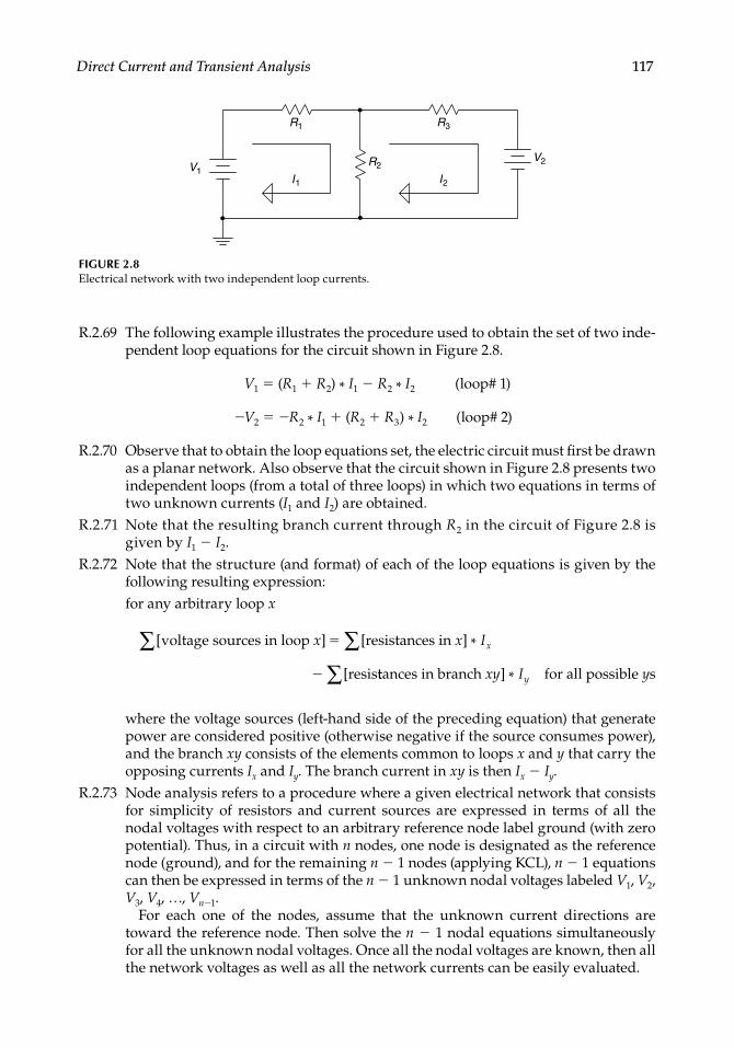
Direct Current and Transient Analysis 117
R.2.69 The following example illustrates the procedure used to obtain the set of two inde-pendent loop equations for the circuit shown in Figure 2.8.
V1 = (R1 + R2) * I1 − R2 * I2 (loop# 1)
−V2 = −R2 * I1 + (R2 + R3) * I2 (loop# 2)
R.2.70 Observe that to obtain the loop equations set, the electric circuit must fi rst be drawn as a planar network. Also observe that the circuit shown in Figure 2.8 presents two independent loops (from a total of three loops) in which two equations in terms of two unknown currents (I1 and I2) are obtained.
R.2.71 Note that the resulting branch current through R2 in the circuit of Figure 2.8 is given by I1 − I2.
R.2.72 Note that the structure (and format) of each of the loop equations is given by the following resulting expression:
for any arbitrary loop x
[ ] [ ] *
[
voltage sources in loop resistances in
resis
x x Ix∑ ∑
ttances in branch for all possible sxy I yy] *∑
where the voltage sources (left-hand side of the preceding equation) that generate power are considered positive (otherwise negative if the source consumes power), and the branch xy consists of the elements common to loops x and y that carry the opposing currents Ix and Iy. The branch current in xy is then Ix − Iy.
R.2.73 Node analysis refers to a procedure where a given electrical network that consists for simplicity of resistors and current sources are expressed in terms of all the nodal voltages with respect to an arbitrary reference node label ground (with zero potential). Thus, in a circuit with n nodes, one node is designated as the reference node (ground), and for the remaining n − 1 nodes (applying KCL), n − 1 equations can then be expressed in terms of the n − 1 unknown nodal voltages labeled V1, V2, V3, V4, …, Vn−1.
For each one of the nodes, assume that the unknown current directions are toward the reference node. Then solve the n − 1 nodal equations simultaneously for all the unknown nodal voltages. Once all the nodal voltages are known, then all the network voltages as well as all the network currents can be easily evaluated.
FIGURE 2.8Electrical network with two independent loop currents.
V1
R1 R3
R2V2
I2I1
CRC_47760_CH002.indd 117CRC_47760_CH002.indd 117 7/23/2008 1:38:38 PM7/23/2008 1:38:38 PM

118 Practical MATLAB® Applications for Engineers
R.2.74 Nodal analysis is more powerful than mesh analysis in the sense that it applies equally well to both planar and nonplanar networks.
For any arbitrary node x, the structure (and format) of the node equation is given by
[ ] [current sources at admittances connected x x∑ between annd y V
x y V
x
y
] *
[ ] *
∑∑ admittances between and for all possiblle sy
where the current sources (left side of equation) are considered positive if its polar-ity points towards x and negative otherwise, and y is a node connected to x through an element (or group of elements) for any y, 1 < y ≤ n – 1.
R.2.75 The following example, a network consisting of three nodes as shown in Figure 2.9, is analyzed using node equations.
ANALYTICAL Solution
The node equations are
For node V1
I
R RV
RV1
1 1 1
1 31
32
* *
For node V2
I
RV
R RV2
31
2 32
1 1 1 * *
R.2.76 Source transformation refers to the fact that any voltage source V in series with a resistor Rs can be replaced by a current source I = V/Rs, in parallel with the same resistor Rs and vice versa as illustrated in Figure 2.10.
R.2.77 An example of source transformation is shown in Figure 2.11, where a voltage source V = 10 V, in series with a resistance Rs = 5 Ω, can be transformed into an equivalent current source I = (10/5) = 2 A in parallel with Rs = 5 Ω.
R.2.78 The superposition theorem states that in a linear DC network, the current through, or voltage across any element is given by the algebraic sum (contributions) of the
FIGURE 2.9Electrical network requiring two node equations.
V1
R1
R3
R2
V2
I2I1
CRC_47760_CH002.indd 118CRC_47760_CH002.indd 118 7/23/2008 1:38:38 PM7/23/2008 1:38:38 PM

Direct Current and Transient Analysis 119
currents or voltages produced independently by each source (current or voltage). The concept of independence means that only one source is considered active, whereas all the other sources (voltage or current) are set to zero.
Recall that when a voltage source is set to zero, the source can be replaced by a short circuit, and similarly, when a current source is set to zero, the source can be replaced by an open circuit.
The superposition theorem states then that in an n source electrical network, the current through or the voltage drop across any arbitrary network element can be obtained by solving n single source networks (where the single source network refers to the original network with only one source at the time whereas all the remaining sources are set to zero) for the variable of interest, which can be a cur-rent or a voltage. The solution is the algebraic sum of the partial solutions (of the single source networks).
Note that the voltage and current polarities (directions) are important when solving each single source network, since the solution is the algebraic sum of the(solutions) contribution of each source.
R.2.79 Thevenin’s theorem states that any two-terminal linear DC network across a load RL can be replaced by two elements: a voltage source called the Thevenin volt-age VTH and a resistor placed in series called the Thevenin resistance RTH. The Thevenin resistance RTH is calculated by setting all the sources to zero, removing the arbitrary load RL (replace it by an open), labeling its terminals aa’, and either calculating or measuring the resistance looking into the terminals (aa’).
The Thevenin voltage VTH is the open-circuit voltage across terminals aa’, after having removed the arbitrary load RL from the original circuit, while preserving all the sources.
R.2.80 Norton’s theorem states that any two-terminal linear DC network can be replaced by two elements, a current source in parallel with a resistor, where the current source is the Norton short-circuit current denoted by IN, and the resistance is the Thevenin resistance RTH.
FIGURE 2.10Equivalent circuits obtained by source transformation.
Rs
I = V/RsArbitrary network
Arbitrary network
V
Rs
FIGURE 2.11Equivalent source transformation circuits as seen through terminals A and B.
Rs = 5 Ω
Rs = 5 Ω
I = V/Rs = 10/5 = 2 A
V = 10 V
A
B
A
B
CRC_47760_CH002.indd 119CRC_47760_CH002.indd 119 7/23/2008 1:38:39 PM7/23/2008 1:38:39 PM

120 Practical MATLAB® Applications for Engineers
The Norton’s short-circuit current IN is the current through terminals aa’, obtained by replacing RL by a short-circuit while preserving all sources.
R.2.81 The equivalent circuits used to evaluate the values of VTH, IN, and RTH are shown in Figure 2.12.
The Thevenin’s and Norton’s equivalent circuits are shown in Figure 2.13.R.2.82 Note that the Thevenin’s and Norton’s equivalent circuits are related by a simple
source transformation as illustrated in Figure 2.14.
FIGURE 2.13(a) Thevenin’s equivalent circuit, (b) Norton’s equivalent circuit.
a ′
aRTH
VTH Arbitrary load RL
a ′
a
RTHArbitrary load RL
IN
(a) (b)
FIGURE 2.12(a) A network with a connected load, (b) Thevenin model for VTH, (c) Norton model for IN, (d) Thevenin–Norton model for RTH.
Arbitrary network
Arbitrary load RLa ′
a
a ′
a ′
a
a
Arbitrary network Vaa ′ = VTH
IN
Arbitrary network
with all sources set to a zero
Arbitrary network
RTH
a ′
a
(a)
(b)
(c)
(d)
CRC_47760_CH002.indd 120CRC_47760_CH002.indd 120 7/23/2008 1:38:39 PM7/23/2008 1:38:39 PM
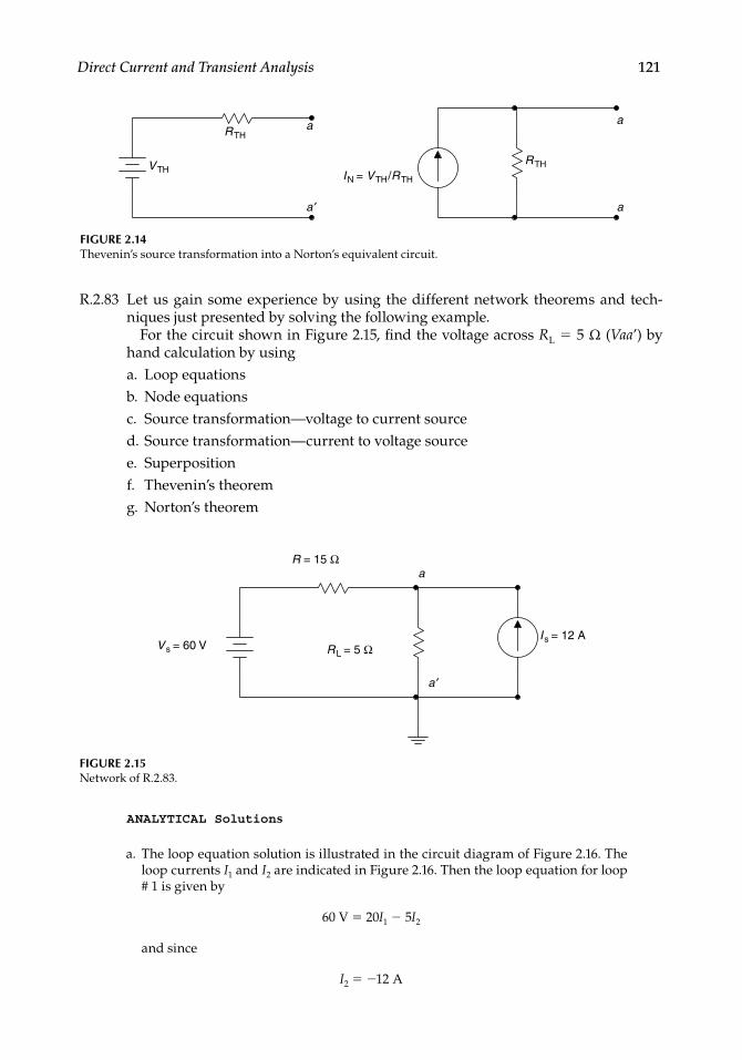
Direct Current and Transient Analysis 121
R.2.83 Let us gain some experience by using the different network theorems and tech-niques just presented by solving the following example.
For the circuit shown in Figure 2.15, fi nd the voltage across RL = 5 Ω (Vaa’) by hand calculation by usinga. Loop equationsb. Node equationsc. Source transformation—voltage to current sourced. Source transformation—current to voltage sourcee. Superpositionf. Thevenin’s theoremg. Norton’s theorem
FIGURE 2.14Thevenin’s source transformation into a Norton’s equivalent circuit.
RTHIN = VTH/RTH
RTH
VTH
a
a ′ a
a
FIGURE 2.15Network of R.2.83.
RL = 5 Ω
R = 15 Ω
Is = 12 AVs = 60 V
a
a ′
ANALYTICAL Solutions
a. The loop equation solution is illustrated in the circuit diagram of Figure 2.16. The loop currents I1 and I2 are indicated in Figure 2.16. Then the loop equation for loop # 1 is given by
60 V = 20I1 − 5I2
and since
I2 = −12 A
CRC_47760_CH002.indd 121CRC_47760_CH002.indd 121 7/23/2008 1:38:39 PM7/23/2008 1:38:39 PM

122 Practical MATLAB® Applications for Engineers
Then
60 V = 20I1 − 5(−12)
60 = 20I1 + 60
60 6020−
I1 0
Then
Vaa’ = 5 Ω ∗ 12 A = 60 V
b. The node equation solution is referred to as the circuit diagram of Figure 2.16. The node equation for node a shown in Figure 2.16 is given below while the reference node is a’ (grounded).
12 A 60
15
115
115
Va
12
415
4Va
12 4
415
Va
16
154
Va
Va = 60 V or Vaa’ = 60 V
c. The voltage source transformation into a current source is shown by the circuit diagram of Figures 2.17 and 2.18, where fi rst the transformation is illustrated (Figure 2.17), followed by the currents’ source combinations (Figure 2.18).
Then
Vaa’ = (15 || 5) 16
Vaa′
(15 * 5 * 16)60 V
15 5
FIGURE 2.16Loop model of network of R.2.83.
RL = 5 Ω
RL = 5 Ω
R = 15 Ω
Is = 12 AVs = 60 V
a
a ′
I1I2
CRC_47760_CH002.indd 122CRC_47760_CH002.indd 122 7/23/2008 1:38:39 PM7/23/2008 1:38:39 PM

Direct Current and Transient Analysis 123
d. The current source transformation into a voltage source is illustrated by the circuit diagram of Figure 2.19. Then
I
60 6020
0
A
therefore
Vaa’ = 60 V
e. The superposition solution is illustrated by the two circuit diagrams shown inFigure 2.20.
FIGURE 2.17The voltage source is transformed in the network of R.2.83.
a
R = 15 ΩIs = 12 A
60/15 = 4 A
a ′
RL = 5 Ω
FIGURE 2.18Current sources are added (combine into an equivalent source) in the network of Figure 2.17.
4+12 = 16 A RL = 5 ΩR = 15 Ω
a ′
a
FIGURE 2.19Current source transforms into a voltage source in the network of R.2.83.
a
a ′
Vs = 60 V 12*5 = 60 VI
RL = 5 ΩR = 15 Ω
CRC_47760_CH002.indd 123CRC_47760_CH002.indd 123 7/23/2008 1:38:40 PM7/23/2008 1:38:40 PM

124 Practical MATLAB® Applications for Engineers
The two single source networks of Figure 2.20 are solved for the voltage dropacross R = 5 Ω labeled Va1 and Va2 and the voltage Vaa’ is then the algebraic sum (Va1 + Va2). The steps involved are indicated as follows:
a. Circuit of Figure 2.15 with Is = 0 b. Circuit of Figure 2.15 with Vs = 0
The voltage Va1 for the circuit shown in Figure 2.20a is given by
Va1 2015
(5 * 60)V (using the voltage divider rule)
The voltage Va2 for the circuit shown in Figure 2.20b is given by
Va2 15 5
45
(15 * 5 * 12)
V
Since Va1 and Va2 have the same polarity
Va = Va1 + Va2 = 15 V + 45 V= 60 V
6. The solution using Thevenin’s theorem is indicated by the circuit diagram ofFigure 2.21. (Note that the load is RL = 5 Ω.)
FIGURE 2.20Superposition models of the network of R.2.83. (a) Circuit of Figure 2.15 with Is = 0, (b) Circuit of Figure 2.15 with Vs = 0.
Vs = 60 V
15
512 A
515
Va2Va1
(a) (b)
FIGURE 2.21Thevenin’s models of the network of R.2.83.
a
a ′
Vs = 60 V
Is = 12 A
R = 15 Ω
CRC_47760_CH002.indd 124CRC_47760_CH002.indd 124 7/23/2008 1:38:40 PM7/23/2008 1:38:40 PM

Direct Current and Transient Analysis 125
Note that the load RL is removed from the circuit of Figure 2.21 and the open voltage Vaa’ is VTH. The evaluation of VTH is given by
Vaa’ = VTH = 60 V + 15 Ω * 12 A = 60 V+ 180 V = 240 V
Then RTH = 15 Ω is obtained by setting all the sources to zero.The resulting Thevenin’s equivalent circuit is shown in Figure 2.22.
Finally, Vaa’ is given by
Vaa′
( * )5 24015 5
60 V
g. Norton’s solution is indicated by the equivalent circuit diagram model of Figure 2.23. The short current IN is then evaluated below
IN A
V15
A A A 1260
12 4 16Ω
The resulting Norton’s equivalent circuit is shown in Figure 2.24.
V Vaa IR NL
′ ( )15 5
V VaaRL
(15 * 5 * 16) V
′
15 560
FIGURE 2.22The Thevenin’s equivalent circuit of the network of R.2.83.
a
VTH = 240 VRL = 5 Ω
RTH = 15 Ω
a ′
FIGURE 2.23The Norton’s equivalent model of the network of R.2.83.
Vs = 60 V
15 Ω
Is = 12 A
INa ′
a
CRC_47760_CH002.indd 125CRC_47760_CH002.indd 125 7/23/2008 1:38:40 PM7/23/2008 1:38:40 PM

126 Practical MATLAB® Applications for Engineers
R.2.84 The maximum power transfer theorem states that maximum power is delivered to a load RL connected to an ideal voltage source Vs connected to a series resistor Rs when the load resistance RL is equal to the resistance Rs as illustrated in the circuit diagram of Figure 2.25.
(Maximum power is delivered to RL when RL = Rs.)R.2.85 For a load RL connected to an arbitrary network, maximum power is delivered to
the load RL, where RL is calculated in the following way:a. The load is removed and replaced by an open circuit (with terminals aa’).b. Calculate the Thevenin’s equivalent resistance RTH by looking into the open ter-
minals (aa’).c. Maximum power is delivered to the load by adjusting RL to be equal to RTH.
R.2.86 Note that the maximum power transfer theorem holds for the case where RTH is fi xed and RL is allowed to vary. If RL is fi xed but RTH is allowed to vary, then maximum power delivered to RL will not occur when RL is equal to RTH, but rather when RTH = 0.
R.2.87 For the example presented in R.2.83 referred to as Figure 2.15, maximum power is delivered to the load RL (5 Ω) by changing (increasing) RL to 15 Ω. The resulting Thevenin’s equivalent circuit of the given network as well as the new load RL is shown in Figure 2.26.
The maximum power delivered to RL is then given by
PRL-max
V
60 W ( )30
15
2
R.2.88 If a circuit is purely resistive with no energy-storing elements (L or G) and switch-ing occurring, then there will be no transient behavior, and current and voltages
FIGURE 2.24The Norton’s equivalent circuit of the network of R.2.83.
RL = 5 Ω
RTH = 15 Ω
IN = 16 A
a ′
a
FIGURE 2.25Maximum power delivered to RL when RL = Rs.
RL
Rs
Vs
CRC_47760_CH002.indd 126CRC_47760_CH002.indd 126 7/23/2008 1:38:41 PM7/23/2008 1:38:41 PM

Direct Current and Transient Analysis 127
reach a steady state instantaneously. In contrast, if storing energy elements are present in a circuit, such as inductors or capacitors, and switching occurs, then transient takes place due to the trapped network voltages and currents, and it takes time to settle into the new stable values.
In brief, transients exist in a circuit if and only if, at any time, a sudden change is made (switched) and energy-storing devices are present.
R.2.89 Transient solutions involve differential equations in which initial conditions must be considered. These solutions require the inclusion of the energy-storing devices (capacitors and inductors) as well as the trapped conditions.
R.2.90 Transient solutions involve either growth or decay time exponentials, and are dependent on the exponential coeffi cient referred as the network time constant (τ).
R.2.91 The time constant can be either RC or L/R or a combination or superposition of time constants for the case of more complex circuits.
R.2.92 The time constant (τ) is the time the circuit requires to complete 63.2% of the change (or discharge) that ultimately takes place. Practical considerations are associated with the time constant, for example, four or fi ve time constants is the time that a circuit needs to reach the steady-state conditions, and after that time, all transients die out or are no longer present.
R.2.93 The transient solution of a given circuit depends on the number of independent energy-storing elements (capacitors and inductors), and not on the number of the network loops or nodes. The reader should observe that capacitors or inductors in series or parallel are not independent, since they can easily be combined. Similarly, a delta (∆) or Y connection consisting of three inductors or three capacitors, one in each branch, leads to just two independent energy-storing elements, since the third element depends on the value of the other two.
R.2.94 Electric circuits with one capacitor or inductor lead to fi rst-order ordinary differ-ential equations, regardless of the structure or complexity of the circuit. Complex circuits with only one type of energy-storing device can be analyzed by using Thevenin’s theorem, assuming that the load is the energy-storing element.
R.2.95 Let us start the transient analysis by considering the RL series circuit shown in Figure 2.27. The switch shown in the circuit closes at t = 0 (it is open for t < 0), and let us assume that the coil is discharged, that is, i(0) = 0. Then by applying KVL, a fi rst-order linear differential equation is obtained, and then solved in terms of the unknown current i(t), illustrated as follows:
Ri t L
di tdt
V( )( )
FIGURE 2.26Load RL is increased to 15 Ω from 5 Ω (potentiometer) for maximum power transfer of the network of R.2.83.
VTH = 60 VRL = 15 Ω
RTH = 15 Ω
CRC_47760_CH002.indd 127CRC_47760_CH002.indd 127 7/23/2008 1:38:41 PM7/23/2008 1:38:41 PM

128 Practical MATLAB® Applications for Engineers
solving for i(t) results in
i t
VR
e tLR
t( ) ( )/ 1 τ for 0 with
R.2.96 When a sudden voltage V is applied to a simple-series RL circuit, a transient con-dition results (recall that the inductor controls the current fl ow), and the general current and voltage relations are given by
i t
VR
e t( ) ( )/1
and the voltage across the resistor R is given by
v t V eRt( ) ( )/ 1
and the voltage across the inductor L is given by
v t V v t V V Ve VeL Rt t( ) ( ) ( )/ /
where τ = L/R (s) is the time constant of the circuit. Note that V = vR(t) + vL(t).R.2.97 In an RL circuit in which the inductor is charged and its initial current is Io and
initial voltage across Vo (with no source), the inductor discharges and the current and voltage relations are given by
i t I e
VR
et t( ) * */ / oo
and
v t V eLt( ) * / o
R.2.98 Let us now turn our attention to the RC series circuit shown in Figure 2.28. The switch is open for t < 0, and closes at t = 0, assuming that the capaci-tor is discharged, that is, vC(0) = 0. Then applying KVL (around the loop), the
FIGURE 2.27RL series circuit.
V
R
L
Switch closes at t = 0
i (t )
CRC_47760_CH002.indd 128CRC_47760_CH002.indd 128 7/23/2008 1:38:42 PM7/23/2008 1:38:42 PM

Direct Current and Transient Analysis 129
following fi rst-order linear differential equation is obtained in terms of the unknown loop current i(t) illustrated as follows:
1C
i t dt Ri t V( ) ( ) ∫
then
i t
VR
e t( ) /
where τ = RC.
v t Ve tRt( ) / for 0
and
v t V v t V Ve tC Rt( ) ( ) / for 0
R.2.99 When a sudden DC voltage V is applied to a simple series RC circuit (with vc(0) = 0 V), the capacitor voltage charges up to
vC(t) = V (1 − e−t/)
and the current through C is then given by
iC tt
VR
e( ) /
where τ = RC (s) is the time constant of the circuit.R.2.100 A charged capacitor in an RC circuit with an initial voltage V(0) and no sources,
as indicated in Figure 2.29, discharges with the following current and voltage relations:
v t VoeCt( ) /
FIGURE 2.28RC series circuit.
V
R
C
Switch closes at t = 0
i (t )
CRC_47760_CH002.indd 129CRC_47760_CH002.indd 129 7/23/2008 1:38:42 PM7/23/2008 1:38:42 PM

130 Practical MATLAB® Applications for Engineers
where τ = RC, and
i t
v tR
VR
e tC t( )( ) / 0 for 0
R.2.101 When a circuit switches from one set of conditions to a new set of conditions, there is a transition period where voltages and currents are adjusting to the new conditions. The term transient response is the adjusting transition time from its initial to its fi nal voltage and current values. The transition takes place in the interval 0 ≤ t ≤ 5τ; and the steady-state response refers to the voltages and cur-rents for t > 5τ.
R.2.102 Let us now review and summarize the inductor’s characteristics.There is no voltage drop across an inductor if the current through it is not chang-ing with time. An inductor is, therefore, a short circuit for DC, and vL(t) = 0, for t > 5τ.A fi nite amount of energy can be stored in an inductor even if the voltage across the inductor is zero.An inductor resists abrupt changes in current.An inductor never dissipates energy; it is only capable of storing energy. This statement is true for the ideal inductor; however, it is false for the real inductor, which always possesses some internal resistance.
R.2.103 The capacitor’s characteristics are summarized as follows:The current through the capacitor is zero, if the voltage across it is not changing with time (DC).A fi nite amount of energy can be stored in a capacitor even if the current through the capacitor is zero.A capacitor resists abrupt change in voltage across it.A pure capacitor cannot dissipate energy; it can only store energy.
R.2.104 For example, analyze the circuit shown in Figure 2.30, and write the differential equation for t ≥ 0, if the switch opens at t = 0 after being closed for a long time. Obtain expressions for vC(t) and iR(t) for t > 0.
•
•
••
•
•
••
C R
+
−
vC(0) =V0
v (t )
FIGURE 2.29Charged capacitor in an RC series circuit.
CRC_47760_CH002.indd 130CRC_47760_CH002.indd 130 7/23/2008 1:38:42 PM7/23/2008 1:38:42 PM

Direct Current and Transient Analysis 131
ANALYTICAL Solution
For t < 0, vC(0) = 2 A * 4 Ω = 8 V.For t > 0, the nodal differential equation is given by
C
dv tdt
v tR
C C( ) ( ) 0
where τ = RC. The solution to the preceding differential equation is of the form vC(t) = Ae−t/τ, and by satisfying the initial conditions at t = 0, the following is obtained: vC(0) = 8 = A, then vC(t) = 8e−t/τ V and iR(t) = vC(t)/R = 2e−t/τ (amp).
R.2.105 The RC and RL transient responses are modeled by fi rst-order differential equa-tions. The RLC transient response leads to a second-order differential equation where the roots of its characteristic equation may be complex numbers. Those roots are referred to as the complex natural frequencies of the circuit. The location of the roots on the complex plane determines the form of the transient response of the electric network. Roots located on the left half of the plane represent decay-ing exponentials, whereas roots on the right half of the plane represent growing exponentials.
Complex conjugate roots can be associated with oscillations (sinusoids); and if they are located in the left half of the plane, they are decaying; and in the right half of the plane, they represent growing sinusoids. When the roots are purely imaginary, they are located on the imaginary (jw) axis of the complex plane and represent sustained oscillations.
R.2.106 Oscillations occur in an RLC circuit when R is small, or the ideal case is when R = 0, then oscillations are sustained. Observe that the resistance R controls the energy dissipated (losses) in the form of heat (friction) and is commonly referred to as the damping coeffi cient.
R.2.107 Three distinct cases are encountered in the solution of second-order systems. They are
OverdampedCritical dampedUnderdamped
These cases are analyzed next for both the series and parallel RLC confi gurations.
•••
FIGURE 2.30RC network of R.2.104.
R = 4 Ω
Switch opens at t = 0
C = 1 FI = 2 A
+
−
+
−
CRC_47760_CH002.indd 131CRC_47760_CH002.indd 131 7/23/2008 1:38:42 PM7/23/2008 1:38:42 PM

132 Practical MATLAB® Applications for Engineers
R.2.108 Systems higher than the second order are not considered in this section, but in general, the solution follows the same steps outlined for the second-order system. Higher-order systems arise when there are more than two independent energy-storing elements. The transient response is obtained by solving for the roots of the network characteristic equation that consist of either real numbers, in which case the response consists of exponentials, or complex conjugate, in which case the response consists of sinusoids (decaying or growing).
R.2.109 Let us analyze the source-free parallel RLC circuit shown in Figure 2.31. The nodal differential equation (KCL) is given by
v tR L
v d i to Cdv tdtL
to
t( )( ) ( )
( )
10 ∫
Then differentiating each term with respect to t yields
C
d v tdt R
dv tdt L
v t2
2
1 10
( ) ( )( )
The auxiliary or characteristic equation becomes (see Chapter 7 of Practical MATLAB® Basics for Engineers)
Cs
sR L
2 10
where s = d/dt, and solving for the two roots yields
s1 2
212
12
1,
RC RC LC
Let
w0
1
LC
where w0 is called the resonant frequency, and let
12RC
where α is referred to as the neper frequency,
FIGURE 2.31Source free parallel RLC of R.2.109.
RL C
IL(to)
VC(to)
+
−
CRC_47760_CH002.indd 132CRC_47760_CH002.indd 132 7/23/2008 1:38:43 PM7/23/2008 1:38:43 PM

Direct Current and Transient Analysis 133
and s1 and s2 are referred as the complex frequencies given by
s w1 22
02
,
R.2.110 As mentioned, the natural response of a parallel RLC circuit results in one of the following three cases:a. Overdampedb. Critical dampedc. Underdamped Observe that the elements defi ne the specifi c case.
R.2.111 Let us analyze each case, starting with the overdamped parallel confi guration that occurs for the following condition:
2 2 w0
and since
s w1 2 02
, 2
then
2
02 2
02 0w w
Note that both s1 and s2 are real, distinct, and negative. Then the solution of the differential equation of R.2.109 is of the form
v t A e A es t s t( ) 1 21 2
where A1 and A2 are constants that can be evaluated from the network initial conditions.
R.2.112 The critical-damped parallel case occurs for the following condition:
202 0 w
Therefore both s1 and s2 are equal to −α, and α is real and negative. The solution of the differential equation of R.2.109 is then of the form
v t A e A tet t( ) 1 2
where A1 and A2 are constants that can be evaluated from the network initial conditions.
R.2.113 The underdamped parallel case occurs for the following condition:
2 2 0 w
Then s1 and s2 become complex conjugate frequencies, and the response of the differential equation of R.2.109 is of the following form:
v t e A w t A w ttd d( ) [ cos( ) sin( )]
1 2
CRC_47760_CH002.indd 133CRC_47760_CH002.indd 133 7/23/2008 1:38:43 PM7/23/2008 1:38:43 PM

134 Practical MATLAB® Applications for Engineers
where
w wd o 2 2
where A1 and A2 are constants that can be evaluated from the initial network conditions.
R.2.114 Let us now turn our attention to the source-free RLC series circuit shown in Figure 2.32, assuming for simplicity that all the initial conditions are zero.
The loop differential equation of the circuit of Figure 2.32 is given by
10
Ci t dt L
di tdt
R i t( )( )
( ) . ∫
Differentiating every term of the preceding equation with respect to t yields
L
d i tdt
Rdi tdt C
i t2
2
10
( ) ( )( )
or
d i tdt
RL
di tdt
i t2
2
10
( ) ( )( ) .
CL
The preceding equation is a second-order, linear, homogeneous differential equation, and the auxiliary equation is given by
s
RL
s2 10
LC
and the roots of this equation are
s
RL
RL1 2
2
2 21
,
LC
where α = R ___ 2L is referred as the neper frequency, wo = 1 _____ √ ___
LC is the resonant frequency, then s1,2 = −α ± √
_______ α2 − w o 2 are referred to as the complex network
frequencies.
FIGURE 2.32Source free series RLC of R.2.114.
R
L
C
CRC_47760_CH002.indd 134CRC_47760_CH002.indd 134 7/23/2008 1:38:43 PM7/23/2008 1:38:43 PM

Direct Current and Transient Analysis 135
Observe that the term (similar to the parallel case) α2 − w o 2 can be positive, zero,
or negative. Then the respective solutions areOverdampedCritical dampedUnderdamped
R.2.115 The natural overdamped RLC series circuit response occurs for the condition α2 > w o 2 . Then the roots s1 and s2 are real, unequal, and negative numbers, resulting in a solution of the form i(t) = A1e−s1t + A2e−s2t, where the constants A1 and A2 depend
on the initial network conditions ( usually given by i(t = 0) and di(t)
____ dt
t = 0
) .R.2.116 The natural critical-damped RLC series circuit response occurs for the condition
α2 = w o 2 . Then the roots s1 and s2 are real (−α) and repeated, resulting in a solution of the form i(t) = A1e−αt + A2te−αt, where the constants A1 and A2 can be evaluated from the system’s initial conditions.
R.2.117 The natural underdamped RLC series circuit response occurs for the condition α2 < w o 2 . Then the roots s1 and s2 are a complex conjugate pair, resulting in a solu-tion of the form
i t e A w t A w ttd d( ) [ cos( ) sin( )]
1 2
where wd = √ _______
w o 2 − α2 and A1 and A2 are constants that depend on the initial network conditions.
R.2.118 The transient analysis of a circuit that contains more than one loop can be described by a set of differential equations. The set of differential equations may consist of either loop or node equations where the unknowns may be either the loop cur-rents or the node voltages. For example, the set of two loop differential equations (using KVL) for the circuit shown in Figure 2.33 is illustrated, where the two loop currents defi ne the system’s transient response.
•••
FIGURE 2.33Transient electrical network of R.2.118.
R1
R3
R2
L3
L1
L2
i2(t )i1(t )
CRC_47760_CH002.indd 135CRC_47760_CH002.indd 135 7/23/2008 1:38:44 PM7/23/2008 1:38:44 PM

136 Practical MATLAB® Applications for Engineers
ANALYTICAL Solution
The set of loop differential equations are
Loop#1 1 2
11 2 1 2 2 2
2: ( )( )
( ) ( ) ( )( )
L Ldi t
dtR R i t R i t L
di tdt
0
Loop#2:
( )( ) ( )
( )( ) ( ) L
di tdt
R i t L Ldi t
dtR R i t2
12 1 2 3
22 3 2 0
The set of initial (or boundary) current conditions such as i1(t0) = I1 and i2(t0) = I2 must be known to completely specify its response.
R.2.119 Recall that capacitors and inductors can be combined and represented by a single equivalent element depending on the type of connection (series or parallel).
The voltage and current divider rules for capacitors and inductors are stated below.
R.2.120 The voltage divider rule is used to evaluate the voltage drops VL1 and VL2 across the inductors L1 and L2 when connected in series with and applied volt-age Vo across them as shown in Figure 2.34.
VL
LL L
V11
1 2
o
VL
LL L
V22
1 2
o
R.2.121 Let us now consider two inductors L1 and L2 connected in parallel, with a current (source) Io feeding the parallel combination as indicated in Figure 2.35.
FIGURE 2.34Voltage divider rule across inductors in series of R.2.120.
L1
L2
Vo
+
+−
− +
−
VL1
VL2
CRC_47760_CH002.indd 136CRC_47760_CH002.indd 136 7/23/2008 1:38:44 PM7/23/2008 1:38:44 PM

Direct Current and Transient Analysis 137
Then the current divider rule states that the currents IL1 and IL2 are given by
IL
LL L
I12
1 2
o
IL
LL L
I21
1 2
o
R.2.122 Now consider two capacitors C1 and C2 connected in series as shown in Figure 2.36 with and applied voltage Vo across them.
Then the voltages VC1 and VC2 are evaluated by using the voltage divider rule as follows:
V
CC C
VC1 o
2
1 2
V
CC C
VC2 o
1
1 2
FIGURE 2.35Current divider rule for inductors in parallel.
Io
+
−
IL1 IL2 L2L1
FIGURE 2.36Voltage divider rule across capacitors in series.
Vo
VC1
VC2
+
−
+
−
CRC_47760_CH002.indd 137CRC_47760_CH002.indd 137 7/23/2008 1:38:44 PM7/23/2008 1:38:44 PM

138 Practical MATLAB® Applications for Engineers
R.2.123 Finally, consider the two capacitors C1 and C2 connected in parallel with a current (source) Io feeding the parallel combination as shown in Figure 2.37.
The currents IC1 and IC2 are evaluated by using the current divider rule as follows:
I
CC C
IC1 o
1
1 2
I
CC C
IC2 o
2
1 2
2.4 Examples
Example 2.1
1. Determine the charge induced when a current of 1 A passes through a point during 2 min
2. Determine the number of electrons required to build up the charge of part 1
Solve this problem analytically and by using MATLAB.
ANALYTICAL Solution
Charge Q (coulombs) = I * t = 1 A * 2 min * 60 s ____ min
Q = 120 A s = 120 C
The number of electrons required to build up a charge of Q = 120 C is given by
Number of electrons 120 C *
1 electron1.602 10 C19
7 49 10. 19 electrons
FIGURE 2.37Current divider rule for capacitors in parallel.
C1 C2Io
+
−
IC1IC2
CRC_47760_CH002.indd 138CRC_47760_CH002.indd 138 7/23/2008 1:38:45 PM7/23/2008 1:38:45 PM

Direct Current and Transient Analysis 139
MATLAB Solution% Script file: chargeI = 1;T = 2*60;Q = I*T;disp(‘*****************************************************’)disp(‘The charge of 1 amp passing through a point during 2 minutes is :’);disp(Q); disp(‘Coulombs’)format longNe=Q*(1/(1.602*10e-19));disp(‘The number of electrons is:’); disp(Ne)disp(‘*****************************************************’)
>> charge
***********************************************************************The charge of 1 amp passing through a point during 2 minutes is : 120 CoulombsThe number of electrons is: 7.490636704119849e+019***********************************************************************
Example 2.2
Create the MATLAB script fi le series that returns the equivalent resistance (across termi-nals AB) shown in Figure 2.38, where R1 = 10 Ω, R2 = 10 Ω, R3 = 20 Ω, and R4 = 30 Ω.
MATLAB Solution% Script file: seriesResist = [10 10 20 30];Requi = sum(Resist);disp(‘********************************’)disp(‘The equivalent resistance is=’); disp(Requi);disp(‘ Ohms’)disp(‘********************************’)
>> series
******************************************** The equivalent resistance is = 70 Ohms ********************************************
FIGURE 2.38Series connections of R1, R2, R3, and R4 of Example 2.2.
R1 = 10 Ω R2 = 10 Ω R3 = 20 Ω R4 = 30 ΩA
B
CRC_47760_CH002.indd 139CRC_47760_CH002.indd 139 7/23/2008 1:38:45 PM7/23/2008 1:38:45 PM

140 Practical MATLAB® Applications for Engineers
Example 2.3
Create the script fi le parallel that returns the equivalent resistance Req across terminals AB of the circuit shown in Figure 2.39, where R1 = 10 Ω, R2 = 10 Ω, R3 = 20 Ω, R4 = 30 Ω, and R5 = 50 Ω.
MATLAB Solution% Script file: parallelResist = [10 10 20 30 50];ones =[1 1 1 1 1];Re = ones./Resistdisp(‘***************************************************’)disp(‘The admittances (in sie.) are=’);disp(Re)Res = sum(Re);Req = 1/Res;disp (‘The equivalent resistance is given by:’); disp(Req)disp(‘ Ohms ’)disp(‘***************************************************’)
>> parallel
*********************************************************The admittances (in sie.) are = Re = 0.1000 0.1000 0.0500 0.0333 0.0200The equivalent resistance is given by: 3.29670329670330 Ohms*********************************************************
Example 2.4
Color coding is used to specify the resistance values (in ohms) as well as its statistical performance (tolerance and reliability).
The color code of a resistor consists of fi ve color bands, as shown in Figure 2.40, where the fi rst three color bands are used to specify the resistance value and the remaining two bands are used to specify their statistical performance.
Each color band represents a numerical value defi ned in Table 2.2.
FIGURE 2.39Parallel connection of R1, R2, R3, R4, and R5 of Example 2.3.
R1 = 10 Ω R2 = 10 Ω R3 = 20 Ω R4 = 30 Ω R5 = 50 Ω
A
B
CRC_47760_CH002.indd 140CRC_47760_CH002.indd 140 7/23/2008 1:38:45 PM7/23/2008 1:38:45 PM

Direct Current and Transient Analysis 141
The value of an arbitrary color-coded resistor R is specifi ed by the following rules:
1. The fi rst (A) and the second (B) band represent the fi rst (A) and the second digit (B), of the value R.
2. The third color band (C) represents a multiplication factor of 10 raised to the power C (10C ), with unit ohms (Ω).
3. The fourth band (D) gives an index of the manufacturer’s tolerance given by [±(AB) * 10C * D].
4. The fi fth color band (E) gives an index of the manufacturer’s component reliability, which represents the probability of failure of R per the fi rst 1000 hours of use.
The nominal value of an arbitrary color-coded resistor R is given by
R = (AB) * 10C
The tolerance of the resistor R would be bounded by
(AB) * 10C − (AB) * 10C * D ≤ R ≤ (AB) * 10C + (AB) * 10C * D
Finally, the reliability of the resistor R is given either by E or E%, and that quantity indi-cates the probability of failure of R during the fi rst 1000 hours of usage.
For example, let a resistor R be defi ned by the following color bands:
Band 1 = Brown (A)Band 2 = Black (B)Band 3 = Orange (C)Band 4 = Silver (D)Band 5 = Brown (E)
TABLE 2.2
Band 1 (First Digit)
Band 2 (Second Digit)
Band 3 (Multiplying Factor)
Band 4 (Tolerance)
Band 5 (Reliability)
Brown = 1 Black = 0 Silver = −2 Gold = 0.05 Brown = 0.01Red = 2 Brown = 1 Gold = −1 Silver = 0.10 Red = 0.001Orange = 3 Orange = 3 Black = 0 None = 0.20 Orange = 0.0001Yellow = 4 Yellow = 4 Brown = 1 Yellow = 0.00001Green = 5 Green = 5 Red = 2Blue = 6 Blue = 6 Orange = 3Violet = 7 Violet = 7 Yellow = 4Gray = 8 Gray = 8 Green = 5White = 9 White = 9 Blue = 6
Violet = 7Gray = 8White = 9
FIGURE 2.40Resistor color bands.
1 2 3 4 5
CRC_47760_CH002.indd 141CRC_47760_CH002.indd 141 7/23/2008 1:38:45 PM7/23/2008 1:38:45 PM

142 Practical MATLAB® Applications for Engineers
ANALYTICAL Solution
From Table 2.2, the nominal value of R is given by
R = 10 * 103 = 10 k
and the range of the resistor R (tolerance) is given by
(10 * 103) − (10 * 103 * 0.1) ≤ R ≤ (10 * 103) + (10 * 103 * 0.1)
then
9,000 ≤ R ≤ 11,000
The fi fth color band indicates the reliability of R, that is, 0.01. In the present case, it indi-cates that one in every 100 resistors would fail during the fi rst 1000 hours of usage.
Having defi ned the color code of resistors, we next proceed to write the MATLAB script fi le color_code, which returns the nominal value of a given resistor R, its tolerance and reliability factor, given its color-coded specs. The program is then tested for the resistor with the following color specs: brown, green, orange, silver, and red.
MATLAB Solution% Script file: color _ code% Color Code ProgramColor1 = char(‘Brown=1’, ‘Red=2’, ‘Orange=3’, ‘Yellow=4’, ‘Green=5’,’Blue=6’,
‘Violet=7’, ‘Gray=8’,’White=9’);
disp (‘The first color band, with its numerical values are given below:’);disp (Color1)A=input(‘Enter the numerical value of the first band, A=’);disp(‘ ’)Color2=char(‘Black=0’, Color1);disp(‘The second color band, with its numerical values are given below:’);disp(Color2)B=input(‘Enter the numerical value of the second ban, B=’);disp(‘ ’)Color3=char(‘Silver=-2’, ‘Gold=-1’, Color2);disp(‘The third color band, with its numerical values are given below:’);disp(Color3)C=input(‘Enter the numerical value of the third band, C=’);disp(‘ ’)Color4=char(‘Gold=0.05’, ‘Silver=0.1’,’Noband=0.2’);disp(‘The forth color band, with its numerical values are given below:’);disp(Color4)D=input(‘Enter the numerical value of the fourth band, D=’);disp(‘ ’)Color5=char(‘Brown=0.01’, ‘Red=0.001’,’Orange=0.0001’,’Yellow=0.00001’);disp(‘The fifth color band, with its numerical values are given below: ‘);disp(Color5)E=input(‘Enter the numerical value of the fifth band, E=’);disp(‘ ’)R=(A*10+B)*10^C;Rmin=R-R*D;Rmax=R+R*D;
CRC_47760_CH002.indd 142CRC_47760_CH002.indd 142 7/23/2008 1:38:46 PM7/23/2008 1:38:46 PM

Direct Current and Transient Analysis 143
Relia=100000*E;disp(‘**************************************************************’)disp(‘****************R E S U L T S *******************************’)disp(‘**************************************************************’)disp([‘The nominal value of R is ‘, num2str(R),’ohms’])disp([‘The range of R (tolerance)is between ‘,num2str(Rmin),’ and ‘, num2str(Rmax),’ Ohms’])disp([‘The statistical number of failure (reliability) is ‘,num2str(Relia),’ for every 100,000 resistors per 1000 hours of use’])disp(‘**************************************************************’)
The script fi le color_code is now tested for the resistor R defi ned by the following color bands: brown, green, orange, silver, and red.
>> color _ code
The first color band, with its numerical values are given below: Brown=1 Red=2 Orange=3 Yellow=4 Green=5 Blue=6 Violet=7 Gray=8 White=9 Enter the numerical value of the first band, A=1
The second color band, with its numerical values are given below: Black=0 Brown=1 Red=2 Orange=3 Yellow=4 Green=5 Blue=6 Violet=7 Gray=8 White=9 Enter the numerical value of the second ban, B=5
The third color band, with its numerical values are given below: Silver=-2 Gold=-1 Black=0 Brown=1 Red=2 Orange=3 Yellow=4 Green=5 Blue=6 Violet=7 Gray=8 White=9 Enter the numerical value of the third band, C=3 The fourth color band, with its numerical values are given below: Gold=0.05 Silver=0.1
CRC_47760_CH002.indd 143CRC_47760_CH002.indd 143 7/23/2008 1:38:46 PM7/23/2008 1:38:46 PM

144 Practical MATLAB® Applications for Engineers
Noband=0.2 Enter the numerical value of the fourth band, D=0.1
The fifth color band, with its numerical values are given below: Brown=0.01 Red=0.001 Orange=0.0001 Yellow=0.00001 Enter the numerical value of the fifth band, E=0.001
************************************************************************************************R E S U L T S**********************************************************************************************The nominal value of R is 15000 ohmsThe range of R (tolerance) is between 13500 and 16500 OhmsThe statistical number of failure (reliability) is 100 for every 100,000 resistors per 1000 hours of use********************************************************************
The reader is encouraged to run and test the preceding program for the three color-coded resistors, given in Table 2.3, and for any arbitrary color-coded resistance.
TABLE 2.3
Examples of Color Coded Resistors
Band 1 Band 2 Band 3 Band 4 Band 5
Yellow Red Orange Silver YellowGray White Violet Gold OrangeRed Green Black No band Red
Example 2.5
Solve by hand and by using MATLAB for the energies stored in the capacitors C1 = 1 F and C2 = 2 F shown in the circuit diagram of Figure 2.41 expressed in the following units:
1. Joules 2. British thermal units 3. Foot pound 4. Watt hour
See R.2.36 for unit conversions.
ANALYTICAL Solution
The equivalent DC circuit of Figure 2.41 is redrawn in Figure 2.42
1. V
V V R R R
W C V
C
C R
C
1
2 2
1 1
10 V
V
( /( )) * ( * )/
( / ) * *
2 1 2 10 2 10 5 4
1 2
+
112 2
22 2
1 2 1 10 50
1 2 1 2 2 4 16
( / ) * *
( / ) * * ( / ) * *
J
J2 2W C VC
2.
W
W
1
2
Btu
Btu
50 1055 0 0474
16 1055 0 0152
/ .
/ .
CRC_47760_CH002.indd 144CRC_47760_CH002.indd 144 7/23/2008 1:38:46 PM7/23/2008 1:38:46 PM

Direct Current and Transient Analysis 145
3. WW
1 f
2 f
ft lb
ft lb
50 0 737 36 85
16 0 737 11 79
* . .
* . .
⋅
⋅
4. WW
1
2
kW h
kW
50 3 6 10 0 0000138
16 3 6 10 0 00000444
6
6
/ . * .
/ . * .
hh
MATLAB Solution>> R1=3; R2=2; C1=1; C2=2; VC=10;>> VC1=VC; VC2=(R2/(R1+R2))*VC;>> W1 _ J=0.5*C1*VC1 2,W2 _ J=0.5*C2*VC2^2
W1 _ J = 50 W2 _ J = 16
FIGURE 2.41Electrical network of Example 2.5.
R3 = 4 Ω
R1 = 3 Ω
R2 = 2 Ω
C1 = 1 F
C2 = 2 F
V = 10 V
FIGURE 2.42Equivalent DC circuit of Figure 2.41.
VC1 =10 V
VC2 =VR2
R1 = 3 Ω R2 = 2 Ω
C1 = 1 F
V = 10 V
CRC_47760_CH002.indd 145CRC_47760_CH002.indd 145 7/23/2008 1:38:46 PM7/23/2008 1:38:46 PM

146 Practical MATLAB® Applications for Engineers
>> W1BTU=W1J/1055, W2BTU=W2J/1055
W1 _ BTU = 0.0474 W2 _ BTU = 0.0152
>> W1 _ ftlbf =W1J*0.737,W2 _ ft1bf=W2J*0.737
W1 _ ft1bf = 36.8500 W2 _ ft1bf = 11.7920
>> W1 _ Kwh=W1J/3.6*10 -6, W2 _ Kwh=W2J/3.6*10 -6
W1 _ Kwh = 1.3889e-005 W2 _ Kwh = 4.4444e-006
Example 2.6
Create the script fi le linearity that verifi es the linear relation between the currentand voltage in a resistive circuit (Ohm’s law), and the nonlinearity of its power forthe circuit shown in Figure 2.43, where the applied voltage V0 varies over the range10 V ≤ V0 ≤ 1000 V in linear increments of 10 V by obtaining the following plots:
1. V0 versus I 2. V0 versus PR (power dissipated by R = 1 kΩ)
FIGURE 2.43Network of Example 2.6.
1 kΩ
V0
l
−
+
MATLAB Solution%Script file: linearityR=1.0e3;V=10:10:1000;I=V./R;P=I.*V;subplot(2,1,1)plot (V,I*1000)title(‘Current vs. Voltage’)xlabel(‘Voltage (Volts)’)ylabel(‘Current (mA)’)subplot(2,1,2)plot (V,P)title(‘Power vs. Voltage’)xlabel(‘Voltage (Volts)’)ylabel(‘Power (watts)’)
The script fi le linearity is executed and the results are shown in Figure 2.44.
CRC_47760_CH002.indd 146CRC_47760_CH002.indd 146 7/23/2008 1:38:47 PM7/23/2008 1:38:47 PM

Direct Current and Transient Analysis 147
Example 2.7
Analyze the circuit shown in Figure 2.43 for the case where the applied voltage source is constant at V0 = 250 V, but the resistance (R) varies over the range 200 Ω ≤ R ≤ 2 kΩ in linear increments of 10 Ω. Obtain plots of
1. I versus R 2. PR versus R
MATLAB Solution>> V = 250;>> R = 200:10:2000;>> I = V./R;>> P = I.*V;>> plot(R,I*1000,R,P) % current in mA>> title(‘Current and Power vs Resistance’)>> xlabel(‘Resistance (Ohms)’), ylabel(‘Current (mA), Power(Watts)’)>> grid on>> gtext (‘Current’) % place the text ‘Current’ and ‘Power’>> gtext (‘Power’) % control text by mouse >> % plots are shown in Figure 2.45
Note that by increasing R, the current I decreases. Since PR = I2R, increasing R dec reases I, where I is the dominant variable. Then by increasing R, the power PR decreases.
FIGURE 2.44Plots of Example 2.6.
0 100 200 300 400 500 600 700 800 900 1000
0 100 200 300 400 500 600 700 800 900 1000
Current versus Voltage
Voltage (Volts)
Voltage (Volts)0
200
400
600
800
1000
0
200
400
600
800
1000
Power versus Voltage
Pow
er (
wat
ts)
Cur
rent
(m
A)
CRC_47760_CH002.indd 147CRC_47760_CH002.indd 147 7/23/2008 1:38:47 PM7/23/2008 1:38:47 PM

148 Practical MATLAB® Applications for Engineers
Example 2.8
Analyze the circuit diagram shown in Figure 2.46, over the range 0 ≤ R2 ≤ 10 kΩ, in linear increments of 10 Ω by returning the following plots:
1. R2 versus I 2. R2 versus V2
3. R2 versus V1
FIGURE 2.45Plots of Example 2.7.
Current and Power versus Resistance
Current
Power
1400
1200
1000
800
Cur
rent
(m
A),
Pow
er (
Wat
ts)
600
400
200
200 400 600 800 1000 1200
Resistance (Ohms)
1400 1600 1800 20000
FIGURE 2.46Network of Example 2.8.
R1 = 1 kΩ
V0 = 10 V
-
+
−R2
V2
V1I
MATLAB Solution>> R1 = 1.0e3;>> V = 10;>> R2 = 0:10:10000; >> I = V./(R1+R2);>> subplot (3,1,1)
CRC_47760_CH002.indd 148CRC_47760_CH002.indd 148 7/23/2008 1:38:47 PM7/23/2008 1:38:47 PM

Direct Current and Transient Analysis 149
>> plot (R2,I*1.0e3) % current in ma>> title (‘Current I, Voltage V2, and Voltage V1 vs R2’); >> ylabel (‘Current I (mA)’)>> grid on; V2 = R2.*I;>> subplot(3,1,2)>> plot (R2,V2)>> ylabel (‘Voltage V2 (Volts)’)>> grid on>> subplot (3,1,3)>> V1 = R1*I; plot(R2,V1)>> xlabel (‘Resistance R2(Ohms)’),>> ylabel (‘voltage V1(Volts)’)>> grid on; >> % plots are shown in Figure 2.47
FIGURE 2.47Plots of Example 2.8.
0 1000 2000 3000 4000 5000 6000 7000 8000 9000 10000
0 1000 2000 3000 4000 5000 6000 7000 8000 9000 10000
00
5
10
0
5
10
0
5
Cur
rent
I (m
A)
Vol
tage
V2
(Vol
ts)
Vol
tage
V1
(Vol
ts)
10
1000 2000 3000 4000 5000 6000
Resistance R2 (Ohms)
7000 8000 9000 10000
Current I, Voltage V2, and Voltage V1 versus R2
It is left as an exercise for the reader to verify that V0 = 10 V = V1 + V2, for any value of R2 satisfying KVL.
Example 2.9
Write a program that analyzes the circuit shown in Figure 2.48, over the range 0 Ω ≤ R3 ≤ 500 Ω, in linear increments of 10 Ω by returning the following plots:
1. R3 versus I 2. R3 versus I2
3. R3 versus I3
4. From the preceding plots, indicate which current is the least and the most affected by the variations of (potentiometer) R3
CRC_47760_CH002.indd 149CRC_47760_CH002.indd 149 7/23/2008 1:38:47 PM7/23/2008 1:38:47 PM

150 Practical MATLAB® Applications for Engineers
MATLAB Solution>> V = 10;>> R1 = 1.0e3;>> R2 = 250;>> R3 = 0:10:500;>> RP = (R2*R3)./(R2+R3); % equivalent resist. of R2 and R3>> RT = R1+RP; % total resistance>> I = V./RT;>> I2 =( I.*R3)./(R2+R3);>> I3 = (I.*R2)./(R2+R3);>> plot (R3,I*1.0e3,’*’, R3, I2*1.0e3, ‘o’,R3,I3*1.0e3,’+’) >> title (‘Currents vs Resistance R3’)>> xlabel (‘Resistance R3 in Ohms’)>> ylabel (‘Currents in Milli-Amperes’)>> legend (‘I’,’I2’,’I3’)>> grid on
FIGURE 2.48Network of Example 2.9.
R1 = 1 kΩ
V0 = 10 V
−
+
I
R2 = 250 Ω
I2 I3R3
0 Ω ≤ R3 ≤ 500 Ω
FIGURE 2.49Plots of Example 2.9.
500450400350300250Resistance R3 in Ohms
2001501005000
1
2
3
4
5
Cur
rent
s in
Mill
i-Am
pere
s
6
7
8
9
10II2I3
Current versus Resistance R3
CRC_47760_CH002.indd 150CRC_47760_CH002.indd 150 7/23/2008 1:38:48 PM7/23/2008 1:38:48 PM

Direct Current and Transient Analysis 151
Observe from Figure 2.49 that when R3 = 250 Ω, I2 = I3. Also observe that the current I is the least affected, whereas the currents I3 and I2 are equally affected by the changes in R3, over the range 0–500 Ω.
Example 2.10
Write a MATLAB program that returns in a tablelike format the resistance values (R) versus length L of a copper wire with a diameter of √
____ 300 mills (the cross-sectional area:
300 CM [circular mills]), over the range 50 ft ≤ L ≤ 500 ft in linear increments of 50 ft, assuming that the temperature remains constant at 20°C.
ANALYTICAL Solution
Recall that the resistance R is given by
RL
A
rho * (at a room temperature of 20°C)
where rho = ρ denotes resistivity in CM Ω/ft, and the rho of copper is 10.37 CM Ω/ft, at 20°C; L defi nes its length in feet; A defi nes the cross-sectional area in CM (circular mills); A (area of a circle) = pi * r2 = π * d2/4; 1000 mills = 1 in. and π/4 sq. mills = 1 CM, then if d is given in mills, A = d2 (in CM).
MATLAB Solution>> L = 50:50:500;>> Rho =10.37;>> A = 300;>> R=Rho.*L./A;>> disp(‘*************************’)>> disp(‘Length (ft) Resit (Ohms)’); results = [L’ R’];>> disp(‘*************************’)>> disp(results)>> disp(‘*************************’)
**************************** Length (ft) Resit (Ohms) **************************** 50.0000 1.7283 100.0000 3.4567 150.0000 5.1850 200.0000 6.9133 250.0000 8.6417 300.0000 10.3700 350.0000 12.0983 400.0000 13.8267 450.0000 15.5550 500.0000 17.2833 ****************************
Example 2.11
Write a program that returns in a tablelike format the resistance of a copper wire of 100 ft long with a fi xed cross-sectional area A = 1 CM as a function of temperature variations (∆T), over the range 0–100°C, in linear increments of ∆T = 10°C.
CRC_47760_CH002.indd 151CRC_47760_CH002.indd 151 7/23/2008 1:38:48 PM7/23/2008 1:38:48 PM

152 Practical MATLAB® Applications for Engineers
ANALYTICAL Solution
Recall thatR
LA
T (1 TC * ) ∆
where ρ is the Greek letter rho, TC = 0.00393 (the temperature coeffi cient of copper), and R = ρ(100/1)(1 + 0.00393 * ∆T).
MATLAB Solution>> T = 0:10:100;>> TC = 0.00393;>> L =100;>> Rho =10.37;>> A=1;>> R= (Rho*100./A)*(1+TC.*T);>> result = [T’ R’];>>disp(‘**********************************’)>> disp(‘Temperature (°C)****Resistance (in Ohms)’); >>disp(‘**********************************’)>>disp(result)>>disp(‘**********************************’)
***************************************************** Temperature (°C)****Resistance (in Ohms)***************************************************** 1.0e+003 0 1.0370 0.0100 1.0778 0.0200 1.1185 0.0300 1.1593 0.0400 1.2000 0.0500 1.2408 0.0600 1.2815 0.0700 1.3223 0.0800 1.3630 0.0900 1.4038 0.1000 1.4445**************************************************
Example 2.12
Let the resistor RL shown in the circuit of Figure 2.50 vary over the range 0 Ω ≤ RL ≤ 10 Ω in linear incremental steps of 0.25 Ω. Write a program that returns the following plots:
1. IL versus RL
2. VL versus RL
3. [PRL = VL * IL] versus RL
For each of the plots, determine the maximum of IL , V2 , and PRL over the range0 Ω ≤ RL ≤ 10 Ω, and verify that PRL-max ≠ IL-max * VL-max and PRL-max < IL-max * VL-max.
MATLAB Solution>> VS =10;>> RL = 0:0.25:10;>> IL = VS./(5+RL);>> VL = IL.*RL;>> subplot (2,2,1)
CRC_47760_CH002.indd 152CRC_47760_CH002.indd 152 7/23/2008 1:38:48 PM7/23/2008 1:38:48 PM

Direct Current and Transient Analysis 153
>> plot (RL, IL)>> grid on>> xlabel(‘Load Resistance RL’), ylabel(‘Current IL’)>> title(‘IL vs. RL’);>> subplot(2,2,2)>> plot(RL,VL)>> grid on>> xlabel(‘Load Resistance RL’), ylabel(‘Voltage VL’)>> title(‘VL vs. RL’);>> subplot(2,2,3)>> P = IL.*VL;>> plot(RL,P)>> grid on>> xlabel(‘Load Resistance RL’), ylabel(‘Power of RL’)>> title(‘Power vs. RL’);>> subplot(2,2,4)>> plot(RL,IL,’o’,RL,VL,’+’,RL,P,’*’)>> grid on>> xlabel(‘Load Resistance RL’), ylabel(‘IL,VL,P=IL*VL’)>> title(‘IL, VL, P vs. RL’);>> legend(‘IL’,’VL’,’P’);>> Imax = max(IL);>> Vmax = max(VL);>> Pmax = max(P);>> Result = [Imax Vmax Pmax];>> disp(‘ ******* R E S U L T S *******”)>> disp(‘************************************************’)>> disp(‘The maximum values for IL, VL, and PL for 0<RL<10 Ohms are:’); >> disp (Result) % the plots are shown in Figure 2.51.>> disp(‘ amps volts watts’)>> disp(‘************************************************’)**************************** R E S U L T S ************************************************************************************* The maximum values for IL, VL, and PL for 0<RL<10 Ohms are: 2.0000 6.6667 5.0000 amps volts watts*****************************************************************
Clearly the results indicate that PRL-max ≠ IL-max * VL-max 5 W ≠ (2 A) * (6.6667 V) and PRL-max = 5 W< IL-max * VL-max = Z * 6.6667 W; the resulting plots are shown in Figure 2.51.
FIGURE 2.50Network of Example 2.12.
RL
Vs = 10 V
5 Ω
−
+
IL
VL
RL = 0 : 0.25 :10
CRC_47760_CH002.indd 153CRC_47760_CH002.indd 153 7/23/2008 1:38:49 PM7/23/2008 1:38:49 PM

154 Practical MATLAB® Applications for Engineers
Example 2.13
Using two loop equations and one node equation, and the matrix operations I = inv(R) * V (where R is the [equivalent] impedance matrix of the network and V the voltage vector), solve for the three branch currents—I1, I2, and I3—shown in the circuit diagram of Figure 2.52.
ANALYTICAL Solution
The node and the two loop equations are shown as follows:
Node A; −I1 + I2 + I3 = 0
Loop# 1; 10 * I1 + 5 * I2 = 10
Loop# 2; −5 * I2 + (10 + 20) * I3 = 0
The preceding equations in matrix form is given by
1 1 110 5 00 5 30
0100
1
2
3
*
I
I
I
Then the 3 × 3 matrix becomes the resistance matrix R, and the voltage V is given by the column vector [0 10 0]T as illustrated by the following matrix equation:
[ ] * [ ] [ ]R I V
then
I = inv (R) * V
FIGURE 2.51Plots of Example 2.12.
2
1.5
1Cur
rent
ILP
ower
of R
L
0.50 5
IL versus RL VL versus RL8
6
4
Vol
tage
VL
2
0
8
6
IL,V
L,P
=IL
∗ VL
IL,VL,P versus RL
IL
4
2
0
Power versus RL
Load Resistance RL Load Resistance RL
Load Resistance RL
Load Resistance RL
10 0 5 10
0 5 1000
1
2
3
4
5
5 10
PVL
CRC_47760_CH002.indd 154CRC_47760_CH002.indd 154 7/23/2008 1:38:49 PM7/23/2008 1:38:49 PM

Direct Current and Transient Analysis 155
MATLAB Solution>> R = [-1 1 1;10 5 0;0 -5 30];>> V = [0;10;0];>> I = inv(R)*V; % Solves for the loop currents>> Result = [I(1) I(2) I(3)];>> % Results are printed>> disp(‘*********************************’);>> disp(‘**********R E S U L T S*********’);>> disp(‘*********************************’);>> disp(‘ The currents I1, I2, I3 are:’); >> disp(Result)>> disp(‘ amp. amp. Amp.’); >> disp(‘*********************************’);
************************************ **********R E S U L T S************ ************************************ The currents I1, I2, I3 are: 0.7000 0.6000 0.1000 amp. amp. amp. ***********************************
Example 2.14
Solve for the loop currents I1 and I2 shown in the circuit diagram of Figure 2.53 (Example 2.13) by using
i. The matrix operation I = R\V ii. The symbolic method iii. Compare the results of i and ii with the solution obtained in Example 2.13
ANALYTICAL Solution
The loop equations are
For loop# I, 15 * I1 − 5 * I2 = 10
For loop# II, −5 * I1 + (5 + 10 + 20) * I2 = 0
FIGURE 2.52Network of Example 2.13.
5 Ω10 V
10 Ω
−
+
I2
10 Ω
20 ΩI1
Loop # 1 Loop # 2
I3
CRC_47760_CH002.indd 155CRC_47760_CH002.indd 155 7/23/2008 1:38:49 PM7/23/2008 1:38:49 PM

156 Practical MATLAB® Applications for Engineers
The matrix equation is then given by
15 55 35
100
1
2
I
I
where the 2 × 2 matrix is the resistance matrix R and [10 0]T represents the column vec-tor V, as indicated by
[ ] [ ]R I V* [ ]
then
[I] = [R] \ [V]
MATLAB Solution>> % part (i) matrix solution>> R = [15 -5;-5 35];>> V = [10;0];>> I = R\V;>> Result = [I(1) I(2) I(1)-I(2)]; % results are printed>> disp(‘**************************************’);>> disp(‘**********R E S U L T S**************’);>> disp(‘ Matrix current solutions’);>> disp(‘**************************************’);>> disp (‘The currents I1, I2, I3 are given by:’); disp(Result)>> disp (‘ amp. amp. amp.’);>> disp(‘**************************************’)************************************************
***************R E S U L T S****************** Matrix current solutions*********************************************** The currents I1, I2, I3 are given by: 0.7000 0.1000 0.6000 amp. amp. amp.************************************************>> % Part (ii); symbolic solution>> sym I1 I2 I3; >> disp(‘**************************************’)
FIGURE 2.53Network of Example 2.14.
A
5 Ω10 V
10 Ω
−
+
I
I2
10 Ω
20 ΩI1
Loop # 1 Loop # 2
CRC_47760_CH002.indd 156CRC_47760_CH002.indd 156 7/23/2008 1:38:49 PM7/23/2008 1:38:49 PM

Direct Current and Transient Analysis 157
>> disp(‘The Symbolic current solutions are given by:’)>> [I1 I2 I3] = solve(‘15*I1-5*I2=10’,’-5*I1+35*I2=0’,’I1-I2=I3’)>> disp(‘*********************************’)
************************************************ The Symbolic current solutions are given by: I1 = 7/10 I2 = 1/10 I3 = 3/5 ************************************************
Note that the results obtained for parts i and ii are equivalent to the solutions obtained in Example 2.13. Also note that the current I3 in Example 2.13 is labeled I2 in Example 2.14.
Example 2.15
Show that the circuit diagrams in Figure 2.54 are equivalent, as seen through the termi-nals labeled a and b.
ANALYTICAL Solution
The circuit diagrams in Figures 2.54a and 2.54b are equivalent due to the equivalent substitutions shown in Figure 2.55. The circuit diagram shown in Figure 2.54b is equivalent to the circuit diagram shown in Figure 2.54c due to the equivalent substitutions indicated in Figure 2.56. The circuit diagram in Figure 2.54c is equivalent to the diagram shown in Figure 2.54d due to the equivalencies shown in Figure 2.57. Finally, the diagram in Figure 2.54d is equivalent to the diagram in Figure 2.54e due to the substitution indicated in Figure 2.58. The equivalencies shown can be evaluated by using the MATLAB programs of Examples 2.2 and 2.3 and are left as an exercise for the reader to verify.
FIGURE 2.54Diagrams of Example 2.15.
ba
(c)
13
12
3
a b5
(e)
ba 1 4
(d)
ba 1
7 5
6
63
(b)
a b
(a)
15
10
30
7
12
4
2
6
4
1
CRC_47760_CH002.indd 157CRC_47760_CH002.indd 157 7/23/2008 1:38:50 PM7/23/2008 1:38:50 PM

158 Practical MATLAB® Applications for Engineers
FIGURE 2.55Equivalent substitutions of Example 2.15 (from Figures 2.54a to 2.54b).
15
(a)
(b)
(c)
2
12
30
10
4
5
3
6
4
FIGURE 2.56Equivalent substitutions of Example 2.15 (from Figures 2.54b to 2.54c).
6
6
3
(b)
7 5 12
(a)
FIGURE 2.57Equivalent substitutions of Example 2.15 (from Figures 2.54c to 2.54d).
1
12
3 3
1
12
6
1
12
6
1 4
FIGURE 2.58Equivalent substitutions of Example 2.15 (from Figures 2.54d to 2.54e).
51 4
CRC_47760_CH002.indd 158CRC_47760_CH002.indd 158 7/23/2008 1:38:50 PM7/23/2008 1:38:50 PM

Direct Current and Transient Analysis 159
Example 2.16
Create the script fi le current_voltage that returns the currents I1, I2, I3, I4, I5, I6, I7, I8, and the voltage Vab shown in the circuit diagram of Figure 2.59 (used in Figure 2.54), given the fact that the current I = 3 A through the 7 Ω resistor.
MATLAB Solution% Script file: current _ voltage clear;clc;I = 3;Vyb = 3*5; % from Figure 2.54aVxb = 12*3; % from Figure 2.54bI1 = Vyb/15;I2 = Vyb/10;I3 = Vyb/30;I8 = Vxb/6; % from Figure 2.54cI4 = (4/16)*I8; % current dividerI5 = (12/16)*I8; I6 = I8/2;I7 = I6;Vab = (I+I8)*5; % from Figure 2.54eresult = [I1 I2 I3 I4 I5 I6 I7 I8];disp(‘**********************************’);disp(‘**********R E S U L T S**********’);disp(‘**********************************’);disp(‘ ‘);disp(‘ The currents I1 I2 I3 I4 I5 I6 I7 and I8 (in amps) are given by:’);disp(result’);disp(‘*********************************’);disp(‘The voltage Vab is:’); disp(Vab); disp(‘volts’)disp(‘*********************************’);
FIGURE 2.59Network of Example 2.16.
15 Ω
7 Ω
12 Ω
1 Ω X
4 Ω 6 Ω
4 Ω
ba
Y
2 Ω
I1
I2
I3
I7
I6
I5
I4
I = 3 A
10 Ω
30 Ω
I8
CRC_47760_CH002.indd 159CRC_47760_CH002.indd 159 7/23/2008 1:38:50 PM7/23/2008 1:38:50 PM

160 Practical MATLAB® Applications for Engineers
The script fi le current_voltage is executed and the results are shown as follows:
>> current _ voltage
***************************************************************************************************R E S U L T S*************************************************************************************************** The currents I1 I2 I3 I4 I5 I6 I7 and I8 (in amps) are given by: 1.0000 1.5000 0.5000 1.5000 4.5000 3.0000 3.0000 6.0000 *********************************************************************** The voltage Vab is: 45 volts***********************************************************************
Example 2.17
For the circuit diagram shown in Figure 2.60
1. Write the three system mesh (loop) equations 2. Arrange the result of part 1 into a matrix equation 3. Using MATLAB, solve for the three loop currents (I1, I2, and I3)
FIGURE 2.60Network of Example 2.17.
I1
2 Ω20 V
I2 I3
Loop # 1 Loop # 2 Loop # 3 10 V
15 V
+−
+−
+ −
4 Ω
6 Ω3 Ω1 Ω
ANALYTICAL Solution
The loop equations are
Loop 1: 20 = 3I1 − 2I2 + 0I3
Loop 2: −15 = −2I1 + 9I2 − 4I3
Loop 3: −10 = 0I1 − 4I2 + 10I3
The resulting matrix equation is
3 2 02 9 4
0 4 10
2015
1
2
3
R
I
I
I
I
*
110
V
CRC_47760_CH002.indd 160CRC_47760_CH002.indd 160 7/23/2008 1:38:50 PM7/23/2008 1:38:50 PM

Direct Current and Transient Analysis 161
MATLAB Solution>> R = [3 -2 0; -2 9 -4; 0 -4 10];>> V = [20; -15; -10];>> I = inv(R)*V;>> Result = [I(1) I(2) I(3)];>> disp(‘***********************************************’)>> disp(‘The loop currents I1, I2 and I3(in amp) are:’);>> disp(Result’);>> disp(‘***********************************************’)
************************************************* The loop currents I1, I2 and I3 (in amp) are: 6.0440 -0.9341 -1.3736 *************************************************
Example 2.18
For the circuit diagram shown in Figure 2.61
1. Write the two node equations (for nodes X and Y ) 2. Arrange the result of part 1 into a matrix equation 3. Use MATLAB to solve for the two voltages (VX and VY)
ANALYTICAL Solution
1. The node equations are
For node X: I1 = ( 1 ___ R1 + 1 ___ R2
) VX – VY or 2 = (1 + 2) VX − VY
For node Y: I2 = –VX + ( 1 ___ R3 + 1 ___ R1
) VY or 3 = −VX + (3 + 1)VY
The two simplifi ed and rearranged node equations are
2 = 3VX − VY
3 = −VX = +4VY
FIGURE 2.61Network of Example 2.18.
X Y R1 = 1 Ω
I2 = 3 A
I1 = 2 A
R3 = 31
+ +
− −
ΩR2 = 21
ΩVX VY
CRC_47760_CH002.indd 161CRC_47760_CH002.indd 161 7/23/2008 1:38:51 PM7/23/2008 1:38:51 PM

162 Practical MATLAB® Applications for Engineers
2. The resulting system nodal matrix equation is given by
3 11 4
23
Y
V
V I
X
Y * V
where Y is the admittance matrix of the network, and the current vector I is given by
I
23
MATLAB Solution>> Y = [3 -1;-1 4];>> I = [2;3];>> V= inv(Y)*I;>> VX = V(1);>> VY =V(2);>> Result = [VX VY];>> disp (‘**********************************’)>> disp (‘The voltage drops Vx and Vy (in volts) are given by:’); >> disp (Result)>> disp (‘**********************************’)
************************************************************ The nodal voltages Vx and Vy (in volts) are given by: 1.0000 1.0000 ************************************************************
Example 2.19
The switch shown in the circuit diagram in Figure 2.62 has been in position a for a long time. At t = 0, the switch is moved to position b where it remains for 2 s and then moves back to position a, where it remains indefi nitely.
1. Obtain analytical expressions for vC(t) and iC(t) for all t 2. Use MATLAB to obtain plots over the range 0 s ≤ t ≤ 10 s of
a. The voltage vC(t) versus t b. The current iC(t) versus t
FIGURE 2.62Network of Example 2.19.
b
a
R3 = 3 ΩR2 = 1 Ω
R1 = 7 Ω
V0 = 100 V
C = 0.5 F
iC(t )
vC(t )
+
−
CRC_47760_CH002.indd 162CRC_47760_CH002.indd 162 7/23/2008 1:38:51 PM7/23/2008 1:38:51 PM

Direct Current and Transient Analysis 163
ANALYTICAL Solution
For t < 0, the switch is in position a. Therefore,
vc(t) = 0
and
ic(t) = 0
For 0 < t < (t1 = 2) seconds, the switch is in position b. Then,
v t V eCt( ) ( )/ 0 1 1
and
i t
V v tR RC
C( )( )
0
1 3
where τ1 = (R1 + R3) * C = 10 Ω * 0.5 F = 5 s.
At time t = t1 = 2 s, the voltage across the capacitor is
v t V V eC C( ) ( )max/
1 021 1
For t > (t1 = 2 s), the switch is back in position a. Then
v t V eC Ct t( ) *max
( )/ 1 2
and
i t
v tR RC
C( )( )
3 2
where τ2 = (R2 + R3) * C = 4 Ω * 0.5 F = 2 s.
MATLAB Solution>> V = 100; R1 =7; R2 =1; R3=3; C =0.5; % circuit elements>> tau1 = (R1+R3)*C % time constant #1
tau1 = 5
>> tau2 = (R2+R3)*C % time constant #2
tau2 = 2
>> for k =1:40 t(k) = k/20; % 0 < t < 2 v(k) = V*(1-exp(-t(k)/tau1)); i(k) = (V-v(k))/(R1+R2); end
CRC_47760_CH002.indd 163CRC_47760_CH002.indd 163 7/23/2008 1:38:51 PM7/23/2008 1:38:51 PM

164 Practical MATLAB® Applications for Engineers
>> Vmax = v(40)
Vmax = 32.9680
>> for k=41:200 t(k)=k/20; % 2 < t < 10 v(k)=Vmax*exp(-(t(k)-t(40))/tau2); t(40)=40/20=2sec=t1 i(k)= -v(k)/(R2+R3); end>> % plot the Voltage VC(t)>> subplot(2,1,1)>> plot(t,v)>> axis([0 10 0 40]);>> title (‘Transients in the circuit of Fig 2.62’)>> xlabel(‘time in sec’), ylabel(‘Voltage vc(t)’)>> grid on>> % plot the current IC (t)>> subplot(2,1,2)>> plot(t,i)>> axis([0 10 -13 15]);>> xlabel(‘time in sec’),ylabel(‘Current ic(t)’)>> grid on
The plots of the Voltage vc(t) and the Current ic(t) versus t are shown in Figure 2.63.
FIGURE 2.63Transient plots of Example 2.19.
40
30
20
10
00 1 2 3 4 5
time in sec
6 7 8 9 10
0
−10
−5
0
Cur
rent
ic(t
)V
olta
ge v
c(t)
5
10
15
1 2 3 4 5
time in sec
6 7 8 9 10
Transients in the circuit of Fig. 2.62
CRC_47760_CH002.indd 164CRC_47760_CH002.indd 164 7/23/2008 1:38:52 PM7/23/2008 1:38:52 PM

Direct Current and Transient Analysis 165
Example 2.20
The switch shown in Figure 2.64 has been at position a for a very long time. At t = 0, the switch is moved to position b where it remains for 2 s and then moves back to position a where it remains indefi nitely.
1. Obtain analytical expressions of i1(t), i2(t), i3(t), and vL(t) for all t. 2. Create the script fi le analysis_exam that returns the following:
a. The network time constants b. The maximum currents I1, I2, and I3
c. The maximum voltage drop across L d. The current plots of i1(t) versus t, i2(t) versus t, and i3(t) versus t over the range
0 s ≤ t ≤ 5 s e. The voltage plot vL(t) versus t over the range 0 s ≤ t ≤ 5 s
3. If the applied source voltage is V0 = 100 V, can the voltage drop across L exceed 100 V?
ANALYTICAL Solution
For t < 0, the switch has been in position a for a long time, then
i1(t) = i2(t) = i3(t) = 0
and vL(t) = 0
During the interval 0 s < t < 2 s, the switch is in position b. Therefore,
i t
VR
e t1
1
1( ) * ( )/ 0
eq
1
i t
RR R
i t23
2 31( ) * ( )
i t
RR R
i t32
2 31( ) * ( )
FIGURE 2.64Network of Example 2.20.
b
a
L = 10 H
i1(t )
i2(t )i3(t )
VL(t )
R1 = 8 Ω
R2 = 6 ΩR3 = 3 ΩR4 = 18 ΩV0 = 100 V
+
−
CRC_47760_CH002.indd 165CRC_47760_CH002.indd 165 7/23/2008 1:38:52 PM7/23/2008 1:38:52 PM

166 Practical MATLAB® Applications for Engineers
and
v t V i t RL( ) ( ) * 1 1eq
where
R R R R R
R RR Req1 1 2 3 1
2 3
2 3
86 36 3
8 2 10
( || ) * *
and
1 = L/Req1 = 10 H/10 = 1 s
At t = t1 = 2 s, the current i1(t1) is at its maximum as given by
I i t
VR
e1 11
22 1 1max
/( ) * ( ) 0
eq
At t = 2 s, the switch moves back to position a, where it remains indefi nitely. The branch currents would then be given by
i t I e t t1 1
1 2( ) max( )/
i t
RR R
i t23
2 31( ) * ( )
i t
RR R
i t32
2 31( ) * ( )
and
v t i t RL( ) ( ) * 1 2eq
where
R R R R R
R RR Req2 4 2 3 4
2 3
2 3
186 36 3
18 2 20
( || ) * *
and
2 = L/Req2 = 10 H/20 = 0.5 s
MATLAB Solution% Script file: analysis _ examV=100; R1 = 8; R2 =3; R3 =6; R4 =18; L=10; % circuit elements.Req1 = R1+(R2*R3)/(R2+R3);
CRC_47760_CH002.indd 166CRC_47760_CH002.indd 166 7/23/2008 1:38:52 PM7/23/2008 1:38:52 PM

Direct Current and Transient Analysis 167
Req2 = R4+(R2*R3)/(R2+R3);disp(‘* * * R E S U L T S * * * ‘)disp(‘*****************************’)disp(‘The network time constants are(in sec):’)tau1 = L/Req1 % time constant #1 tau2 = L/Req2 % time constant #2for K=1:40 t(K) = K/20; % 0 < t < 2. I1(K) = (V/Req1)*(1-exp(-t(K)/tau1)); I2(K) = R3*I1(K)/(R2+R3); I3(K) = R2*I1(K)/(R2+R3); VL(K) = V-I1(K)*Req1; enddisp(‘the maximum currents are:’) I1Max = I1(40);for K= 41:100t(K) = K/20; % 2 < t < 5.I1(K) = I1Max*exp(-(t(K)-t(40))/tau2); % t(40) = 40/20 = 2 sec.= t1I2(K) = R3*I1(K)/(R2+R3);I3(K) = R2*I1(K)/(R2+R3);VL(K) = -I1(K)*Req2;end % plots the current i1(t)I1Max= max(I1)Tmax = max(t);subplot(2,2,1)plot(t,I1)axis([0 5 0 10])grid ontitle(‘Current i1(t) vs.t’), ylabel(‘Current in amps’);xlabel(‘time in sec’) % plots the current i2(t)I2Max = max(I2) I3Max=max(I3)subplot(2,2,2)plot(t,I2)axis([0 5 0 6])grid ontitle(‘Current i2(t) vs.t’), ylabel(‘Current in amps’);xlabel(‘time in sec’)subplot(2,2,3) % plots the current i3(t)plot(t,I3)axis([0 5 0 3])grid ontitle(‘Current i3(t) vs. t’), ylabel(‘Current in amps’)xlabel(‘time in seconds’); % plots the voltage vL(t)disp(‘ The magnitude of the maximum voltage across L is:’)VLMax = -max(abs(VL)) subplot(2,2,4)plot(t,VL)axis([0 5 -160 100])grid ontitle(‘Voltage vL(t) vs.t’), xlabel(‘time in seconds’) ylabel(‘Voltage in volts ‘)disp(‘***************************************’)
CRC_47760_CH002.indd 167CRC_47760_CH002.indd 167 7/23/2008 1:38:53 PM7/23/2008 1:38:53 PM

168 Practical MATLAB® Applications for Engineers
The script fi le analysis_exam is executed and the results are shown as follows and in Figure 2.65.
>> analysis _ exam _ 1020
* * * R E S U L T S * * * ***************************The network time constants are (in sec): tau1 = 1 tau2 = 0.5000The maximum currents are:I1Max = 8.6466I2Max = 5.7644I3Max = 2.8822The magnitude of the maximum voltage across L is:VLMax = -156.4762******************************************
FIGURE 2.65Transient plots of Example 2.20.
0−150
−100
−50
0
50
100
0
1
2
Cur
rent
in a
mps
Vol
tage
in v
olts
Cur
rent
in a
mps
3
0
8
6
4
2 Cur
rent
in a
mps
0
6
4
2
10
1 2 3
time in seconds
4 50 1 2 3
time in seconds
4 5
0 1 2 3 4 50 1 2 3 4 5
Current i3(t) versus t
Current i1(t) versus t Current i2(t) versus t
Voltage vL(t) versus t
time in sec time in sec
Observe that the voltage across the inductor vL(t) at t = 2 s is vL(t = 2) = 156.4762 V when the applied (source) voltage is V = 100 V. Observe also that at t = 2 s, I1max = 8.6466 A = I2max + I3max = 5.7644 A + 2.8822 A verifying KCL.
CRC_47760_CH002.indd 168CRC_47760_CH002.indd 168 7/23/2008 1:38:53 PM7/23/2008 1:38:53 PM

Direct Current and Transient Analysis 169
Example 2.21
Assuming that the load is RL, determine the Thevenin’s equivalent circuit of the electri-cal network shown in Figure 2.66 by
a. Hand calculations. b. Creating the script fi le Thevenin that simulates Thevenin’s theorem consisting in
varying RL over the range 1 ≤ RL ≤ 50 Ω, in steps of 1 Ω, and computing the respec-tive powers for each value of RL. Recall that the resistance dissipates maximum power when RL = RTH and its VTH = 2 VRTH.
FIGURE 2.66Network of Example 2.21.
Vs = 100 V
−
+
I
RL
RL = 1 :1:50
a
a ′
R1 = 20 Ω
R2 = 60 Ω
FIGURE 2.67Calculated Thevenin’s equivalent circuit of Example 2.21.
−
+
I
VTH = 75 V RL
a
a′
RTH = 15 Ω
ANALYTICAL Solution
Part a
The VTH and RTH are evaluated by hand.
VTH V
60 10020 60
600080
75*
and
R R RTH
1 2
20 6020 60
120080
15|| *
The calculated Thevenin’s equivalent circuit, as seen through the terminals aa’, is shown in Figure 2.67.
CRC_47760_CH002.indd 169CRC_47760_CH002.indd 169 7/23/2008 1:38:53 PM7/23/2008 1:38:53 PM

170 Practical MATLAB® Applications for Engineers
MATLAB Solution% script file: Thevenin% The Thevenin’s equivalent circuit % can be determined by experimental method % based on the maximum power theorem Vs =100;R1 = 20;R2 =60;RL = 1:1:50; % range of RLRpar = (RL.*R2)./(RL+R2);RT = Rpar + R1;VL = (Rpar.*Vs)./RT;PRL = (VL. 2)./RL;[Pmax,index] = max(PRL);Rth = RL(index);Vth = sqrt(4*Rth*Pmax);%...Display Vth and Rth disp(‘*********************************’);disp(‘*********R E S U L T S**********’);disp(‘*********************************’);disp(‘ ‘);fprintf(‘The Thevenin voltage (in volts) is Vth=%f\n’,Vth);fprintf(‘The Thevenin resistance (in ohms) is Rth=%f\n’,Rth);disp(‘ ‘)disp(‘*********************************’);
The script fi le Thevenin is executed, and the results are shown as follows:
>>Thevenin
******************************************************* *************** R E S U L T S ************************ *******************************************************
The Thevenin voltage (in volts) is Vth =75.000000 The Thevenin resistance (in ohms) is Rth =15.000000
*******************************************************
Note that the calculated results completely agree with the simulated experimental results.
Example 2.22
Analyze the series RLC circuit shown in Figure 2.68, where the current source i(t) is
given by i(t) = ( 2 __ π ) ∑ n=odd
15
( 1 __ n ) sin(n π t). The equation for the current i(t) represents the Fourier
series approximation of a periodic square wave (see Chapter 4 for additional details).
Create the script fi le analysis that returns the following plots:
1. i(t) versus t (verifi es the approximation of the periodic square wave)
2. i2(t) versus t
3. ∫
i(t) dt versus t (verifi es the approximation of the periodic triangular wave)
4. di(t)
____ dt
versus t
CRC_47760_CH002.indd 170CRC_47760_CH002.indd 170 7/23/2008 1:38:53 PM7/23/2008 1:38:53 PM
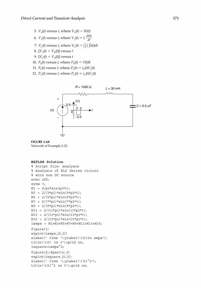
Direct Current and Transient Analysis 171
5. VR(t) versus t, where VR(t) = Ri(t)
6. VL(t) versus t, where VL(t) = L di(t) ____
dt
7. VC(t) versus t, where VC(t) = ( 1 __ C ) ∫
i(t) dt
8. [VL(t) + VR(t)] versus t
9. [VC(t) + VR(t)] versus t
10. PR(t) versus t, where PR(t) = i2(t)R
11. PL(t) versus t, where PL(t) = iL(t)VL(t)
12. PC(t) versus t, where PC(t) = iC(t)VC(t)
FIGURE 2.68Network of Example 2.22.
C = 0.5 µFi (t )
+
−−
L = 30 mHR = 1000 Ω
1 2
−0.5
i (t )
t
0.5
0
MATLAB Solution% Script file: analysis% Analysis of RLC Series circuit% with non DC source echo off;syms t;H1 = 2/pi*sin(pi*t);H3 = 2/(3*pi)*sin(3*pi*t);H5 = 2/(5*pi)*sin(5*pi*t);H7 = 2/(7*pi)*sin(7*pi*t);H9 = 2/(9*pi)*sin(9*pi*t);H11 = 2/(11*pi)*sin(11*pi*t);H13 = 2/(13*pi)*sin(13*pi*t);H15 = 2/(15*pi)*sin(15*pi*t);iamps = H1+H3+H5+H7+H9+H11+H13+H15;
figure(1)ezplot(iamps,[0,3])xlabel(‘ time ‘);ylabel(‘i(t)in amps’);title(‘i(t) vs t’);grid on;isquare=iamps^2;
figure(2);%part(c.2)ezplot(isquare,[0,3])xlabel(‘ time ‘);ylabel(‘i(t) 2’);title(‘i(t) 2 vs t’);grid on;
CRC_47760_CH002.indd 171CRC_47760_CH002.indd 171 7/23/2008 1:38:54 PM7/23/2008 1:38:54 PM

172 Practical MATLAB® Applications for Engineers
figure(3)inti = int(iamps);ezplot (inti,[0,3])xlabel(‘ time ‘);ylabel(‘integral[i(t)]’);title(‘integral[i(t)] vs t’);grid on;
figure(4)diffi = diff(iamps);ezplot(diffi,[0,3])xlabel(‘ time ‘);ylabel(‘d[i(t)/dt]’);title(‘d[i(t)/dt] vs t’);grid on;
figure(5)Vr = 1000*iamps;ezplot(Vr,[0,3])xlabel(‘ time ‘);ylabel(‘Vr(t)in volts’);title(‘Vr(t) vs t’);grid on;
figure(6)Vl = 30e-3*diffi;ezplot(Vl,[0,3])xlabel(‘ time ‘);ylabel(‘VL(t)in volts’);title(‘VL(t) vs t’);grid on;
figure(7)Vc=.5e-6*inti;ezplot(Vc,[0,3])title(‘Vc(t) vs t’)xlabel(‘ time ‘);ylabel(‘Vc(t)in volts’)title(‘ Vc(t) vs t’);grid on;
figure(8)Vlr=Vl+Vr;ezplot(Vlr,[0,3])title(‘[Vr(t)+VL(t)] vs t’);xlabel(‘ time ‘);ylabel(‘[Vr(t)+VL(t)] in volts’);grid on;
figure(9)Vcr=Vc+Vr;ezplot(Vcr,[0,3])title(‘[Vr(t)+Vc(t)] vs t’)xlabel(‘ time ‘);ylabel(‘[Vr(t)+Vc(t)]’);title(‘[Vr(t)+Vc(t)] vs t’);grid on
figure(10)Pr = iamps*Vr;ezplot(Pr,[0,3])title(‘Pr(t) vs t’)xlabel(‘ time ‘)ylabel(‘Pr(t) in watts’);grid on;
figure(11)Pl = iamps*Vl;ezplot(Pl,[0,3])title(‘PL(t) vs t’); xlabel(‘ time ‘);ylabel(‘PL(t)’);grid on
figure(12)Pc = iamps*Vc; ezplot(Pc,[0,3]);
CRC_47760_CH002.indd 172CRC_47760_CH002.indd 172 7/23/2008 1:38:54 PM7/23/2008 1:38:54 PM

Direct Current and Transient Analysis 173
FIGURE 2.69Plot of i(t) of Example 2.22 MATLAB Figure (1).
0 0.5 1 1.5 2 2.5 3
−0.6
−0.4
−0.2
0
0.2
0.4
0.6
time
i(t ) versus t
i(t)
in a
mps
FIGURE 2.70Plot of i(t)2 of Example 2.22 MATLAB Figure (2).
0 0.5 1 1.5 2 2.5 3
0.15
0.2
0.25
0.3
0.35
time
i(t )2 versus t
i(t)
2
title(‘Pc(t) vs t’);xlabel(‘ time ‘);ylabel(‘Pc(t)’);grid on;
The script fi le analysis is executed and the resulting plots are shown in Figures 2.69 through 2.80.
>> analysis
CRC_47760_CH002.indd 173CRC_47760_CH002.indd 173 7/23/2008 1:38:54 PM7/23/2008 1:38:54 PM

174 Practical MATLAB® Applications for Engineers
FIGURE 2.72
Plot of di(t) ____ dt of Example 2.22 MATLAB Figure (4).
0 0.5 1 1.5 2 2.5 3−5
−4
−3
−2
−1
0
1
2
3
4
time
d[i(t)/dt] versus t
d[i(t
)/dt
]
FIGURE 2.71Plot of ∫
i(t)dt of Example 2.22 MATLAB Figure (3).
0 0.5 1 1.5 2 2.5 3
−0.25
−0.2
−0.15
−0.1
−0.05
0
0.05
0.1
0.15
0.2
0.25
time
integral[i(t)] versus t
inte
gral
[i(t)
]
CRC_47760_CH002.indd 174CRC_47760_CH002.indd 174 7/23/2008 1:38:54 PM7/23/2008 1:38:54 PM

Direct Current and Transient Analysis 175
FIGURE 2.73Plot of the voltage across R of Example 2.22 MATLAB Figure (5).
0 0.5 1 1.5 2 2.5 3
−600
−400
−200
0
200
400
600
time
Vr(t) versus t
Vr(
t) in
vol
ts
FIGURE 2.74Plot of the voltage across L of Example 2.22 MATLAB Figure (6).
0 0.5 1 1.5 2 2.5 3−0.15
−0.1
−0.05
0
0.05
0.1
time
VL(t) versus t
VL(
t) in
vol
ts
CRC_47760_CH002.indd 175CRC_47760_CH002.indd 175 7/23/2008 1:38:55 PM7/23/2008 1:38:55 PM

176 Practical MATLAB® Applications for Engineers
FIGURE 2.75Plot of the sum of the voltage across R and L of Example 2.22 Figure (7).
0 0.5 1 1.5 2 2.5 3
−1
−0.5
0
0.5
1
× 10−7
time
Vc(t) versus t
Vc(
t) in
vol
ts
FIGURE 2.76Plot of the voltage across C of Example 2.22 MATLAB Figure (8).
0 0.5 1 1.5 2 2.5 3
−600
−400
−200
0
200
400
600
time
[Vr(t)+VL(t)] versus t
[Vr(
t)+
VL(
t)] i
n vo
lts
CRC_47760_CH002.indd 176CRC_47760_CH002.indd 176 7/23/2008 1:38:55 PM7/23/2008 1:38:55 PM

Direct Current and Transient Analysis 177
FIGURE 2.77Plot of the sum of the voltage across R and C of Example 2.22 Figure (9).
0 0.5 1 1.5 2 2.5 3
−600
−400
−200
0
200
400
600
time
[Vr(t)+Vc(t)] versus t
[Vr(
t)+
Vc(
t)]
FIGURE 2.78Plot of the power of R of Example 2.22 MATLAB Figure (10).
0 0.5 1 1.5 2 2.5 3
150
200
250
300
350
time
Pr(t) versus t
Pr(
t) in
wat
ts
CRC_47760_CH002.indd 177CRC_47760_CH002.indd 177 7/23/2008 1:38:55 PM7/23/2008 1:38:55 PM

178 Practical MATLAB® Applications for Engineers
FIGURE 2.79Plot of the power of L of Example 2.22 MATLAB Figure (11).
0 0.5 1 1.5 2 2.5 3
−0.06
−0.04
−0.02
0
0.02
0.04
0.06
time
PL(t) versus t
PL(
t)
FIGURE 2.80Plot of the power of C of Example 2.22 MATLAB Figure (12).
0 0.5 1 1.5 2 2.5 3
−6
−4
−2
0
2
4
6
×10−8
time
Pc(t) versus t
Pc(
t)
Example 2.23
Determine the current i(t) for t ≥ 0 for each value of R, R = 1, 2, and 5 Ω for the RL circuit diagram shown in Figure 2.81, assuming that the initial current is given by iL(0) = 0 A.
a. By hand calculations b. By creating the script fi le RL that returns the symbolic MATLAB solution of the
loop differential equation, and c. Each of the corresponding plots for i(t) versus t
CRC_47760_CH002.indd 178CRC_47760_CH002.indd 178 7/23/2008 1:38:55 PM7/23/2008 1:38:55 PM

Direct Current and Transient Analysis 179
ANALYTICAL Solution
Part a
The loop differential equation, as well as its current solution i(t), is given as follows:
Ldi tdt
Ri t V( )
( ) 0
then
i tVR
VR
e t Rt( ) 0 0 0 for for 1, 2, and 5
where τ = L/R.
MATLAB Solution% Script file: RL% parts ( b and c )itR _ 1 = dsolve(‘Dy+y =10’,’y(0) = 0’,’t’);itR _ 2 = dsolve(‘Dy+2*y=10’,’y(0)=0’,’t’);itR _ 5 = dsolve(‘Dy+5*y=10’,’y(0)=0’,’t’);disp(‘***************************’);disp(‘The solutions i(t) for R=1,2 and 5 (in Ohms) are:’);disp(‘***************************’);disp(‘***************************’);itR _ 1disp(‘***************************’);itR _ 2disp(‘***************************’);itR _ 5disp(‘***************************’);disp(‘***************************’);ezplot(itR _ 5,[0 3]);hold on;grid on; ezplot(itR _ 2,[0 3]);hold on;ezplot(itR _ 1,[0 3]);hold on;title(‘i(t) vs t for L=1 & R=1,2 and 5’)axis([0 3 0 11]);xlabel(‘time t’);ylabel(‘i(t)’)
FIGURE 2.81Network of Example 2.23.
V0 = 10 V R
L = 1 HSwitch closes at t = 0
i (t )
CRC_47760_CH002.indd 179CRC_47760_CH002.indd 179 7/23/2008 1:38:55 PM7/23/2008 1:38:55 PM

180 Practical MATLAB® Applications for Engineers
The script fi le RL is executed and the results and plots (Figure 2.82) are shown as follows:
>> RL
******************************************************The solutions i(t) for R=1, 2 and 5 (in Ohms) are :************************************************************************************************************itR _ 1 = 10-10*exp(-t)******************************************************itR _ 2 = 5-5*exp(-2*t)*******************************************************itR _ 5 = 2-2*exp(-5*t)************************************************************************************************************
0 0.5 1 1.5 2 2.5 30
1
2
3
4
5
6
7
8
9
10
11
time t
i(t) versus t for L=1 & R=1, 2, and 5
i(t)
time const = 1 sec
time const = 0.5 sec
time const = 0.2 sec
FIGURE 2.82Transient current plots of Example 2.23.
Example 2.24
Create the script fi le RL_vol_plots that returns
1. The expression of vL(t) and plot vL(t) versus t, for t ≥ 0 2. The expression of vR(t) and plot vR(t) versus t, for t ≥ 0
for the circuit shown in Figure 2.81, for the same three resistors: R = 1, 2, and 5 Ω, assuming that the initial current is iL(0) = 0 A.
CRC_47760_CH002.indd 180CRC_47760_CH002.indd 180 7/23/2008 1:38:56 PM7/23/2008 1:38:56 PM

Direct Current and Transient Analysis 181
MATLAB Solution% Script file: RL _ vol _ plots itR _ 1=dsolve(‘Dy+y=10’,’y(0)=0’,’t’);itR _ 2=dsolve(‘Dy+2*y=10’,’y(0)=0’,’t’);itR _ 5=dsolve(‘Dy+5*y=10’,’y(0)=0’,’t’);disp(‘*********** R E S U L T S **************’)disp(‘*****************************************’);disp(‘The voltages across R = 1, 2 and 5 (in Ohms) are:’);disp(‘***************************’);disp(‘***************************’);vr _ 1=itR _ 1*1disp(‘***************************’);vr _ 2=itR _ 2*2disp(‘***************************’);vr _ 5=itR _ 5*5disp(‘***************************’);
figure(1)ezplot(itR _ 1*1,[0 4]);hold onezplot(itR _ 2*2,[0 4]);hold onezplot(itR _ 5*5,[0 4]);hold ongrid on;axis([0 3 0 11])xlabel(‘time t/sec’)ylabel(‘voltage ‘)title(‘Voltages across R for, R=1,2 and 5 ‘)
figure(2)disp(‘***************************’);disp(‘The voltages across L=1’) disp(‘ for R=1,2 and 5 (in Ohms) are:’);disp(‘***************************’);disp(‘***************************’);vlr _ 1=10-itR _ 1*1disp(‘***************************’);vlr _ 2=10-itR _ 2*2disp(‘***************************’);vlr _ 5=10-itR _ 5*5disp(‘***************************’);ezplot(10-itR _ 1*1,[0 4]);hold onezplot(10-itR _ 2*2,[0 4]);hold onezplot(10-itR _ 5*5,[0 4]);hold ongrid on;axis([0 3 0 11])xlabel(‘time t/sec’)ylabel(‘voltage ‘)title(‘Voltages across L=1, for R=1,2 and 5’)
The script fi le RL_vol_plots is executed, and the results and plots are shown as follows:
>> RL _ vol _ plots
*******************R E S U L T S **************************************************************************The voltages across R = 1, 2 and 5 (in Ohms) are:******************************************************
CRC_47760_CH002.indd 181CRC_47760_CH002.indd 181 7/23/2008 1:38:56 PM7/23/2008 1:38:56 PM
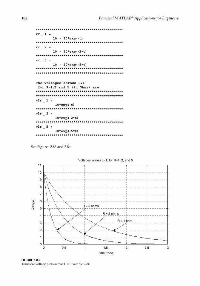
182 Practical MATLAB® Applications for Engineers
********************************************vr _ 1 = 10 - 10*exp(-t)********************************************vr _ 2 = 10 - 10*exp(-2*t)********************************************vr _ 5 = 10 - 10*exp(-5*t)****************************************************************************************
The voltages across L=1 for R=1,2 and 5 (in Ohms) are:****************************************************************************************vlr _ 1 = 10*exp(-t)********************************************vlr _ 2 = 10*exp(-2*t)********************************************vlr _ 5 = 10*exp(-5*t)********************************************
See Figures 2.83 and 2.84.
FIGURE 2.83Transient voltage plots across L of Example 2.24.
0 0.5 1 1.5 2 2.5 30
1
2
3
4
5
6
7
8
9
10
11
time t /sec
Voltages across L=1, for R=1, 2, and 5
volta
ge
R = 1 ohm
R = 2 ohms
R = 5 ohms
CRC_47760_CH002.indd 182CRC_47760_CH002.indd 182 7/23/2008 1:38:56 PM7/23/2008 1:38:56 PM

Direct Current and Transient Analysis 183
Example 2.25
The switch of the circuit diagram shown in Figure 2.85 is open for t < 0, and it closes at t = 0 where it remains indefi nitely. Obtain
1. Analytical expressions for vc(t), vR(t), and i(t) assuming that ic(0) = 0 A, for t ≥ 0. 2. Create the script fi le RC that returns the MATLAB symbolic solutions for vc(t), vR(t),
and i(t) by solving the corresponding loop differential equation for each of the following cases: R = 1, 2, and 5 Ω.
3. The plots of a. vc(t) versus t b. vR(t) versus t c. i(t) versus t
FIGURE 2.84Transient voltage plots across R of Example 2.24.
0 0.5 1 1.5 2 2.5 30
1
2
3
4
5
6
7
8
9
10
11
time t/sec
Voltages across R for, R = 1, 2, and 5
volta
ge
R = 5 ohmsR = 2 ohms
R = 1 ohm
FIGURE 2.85Network of Example 2.25.
V0 = 10 V R
Switch closes at t = 0 C = 0.5 F
ANALYTICAL Solution
The loop differential equation and its solution are given as follows:
RCdv t
dtv t V v t V V e tC
C Ct( )
( ) ( ) 0 0 0 0and for
CRC_47760_CH002.indd 183CRC_47760_CH002.indd 183 7/23/2008 1:38:56 PM7/23/2008 1:38:56 PM

184 Practical MATLAB® Applications for Engineers
then
vR(t) = V0 − vC(t) = Ve−t/ for R = 1, 2, and 5 Ω
and
i t( ) v t
RVR
eR t( ) /0
where τ = RC.
MATLAB Solution% Script file:RCvctR _ 1=dsolve(‘0.5*Dy+y=10’,’y(0)=0’,’t’);vctR _ 2=dsolve(‘Dy+y=10’,’y(0)=0’,’t’);vctR _ 5=dsolve(‘2.5*Dy+y=10’,’y(0)=0’,’t’);disp(‘****************************************’);disp(‘********** R E S U L T S **************’)disp(‘****************************************’);disp(‘The voltages across C for R=1,2 and 5(in volta)are:’);disp(‘****************************************’);vctR _ 1disp(‘****************************************’);vctR _ 2disp(‘****************************************’);vctR _ 5disp(‘****************************************’);
figure(1)ezplot(vctR _ 1,[0 4]);hold onezplot(vctR _ 2,[0 4]);hold onezplot(vctR _ 5,[0 4]);hold ongrid on;axis([0 3 0 11])xlabel(‘time t/sec’)ylabel(‘voltage ‘)title(‘Voltages across C for R=1,2 and 5 are:’)
figure(2)disp(‘The voltages across R’) disp(‘ for R=1,2 and 5 (in volts) are:’);disp(‘****************************************’);vr1=10-vctR _ 1disp(‘****************************************’);vR2=10-vctR _ 2disp(‘****************************************’);vR5=10-vctR _ 5disp(‘****************************************’);ezplot(10-vctR _ 1,[0 4]);hold onezplot(10-vctR _ 2,[0 4]);hold onezplot(10-vctR _ 5,[0 4]);hold on
CRC_47760_CH002.indd 184CRC_47760_CH002.indd 184 7/23/2008 1:38:57 PM7/23/2008 1:38:57 PM

Direct Current and Transient Analysis 185
grid on;axis([0 3 0 11])xlabel(‘time t/sec’)ylabel(‘voltage ‘)title(‘Voltages across R, for R=1,2 and 5’)disp(‘The current i(t) through R=1,2 and 5 (in amps) are:’);disp(‘***************************’);iR1=10-vctR _ 1disp(‘***************************’);iR2=10-vctR _ 2)/2disp(‘***************************’);iR5=(10-vctR _ 5)/5disp(‘***************************’);
figure(3)ezplot(10-vctR _ 1,[0 4]);hold on;ezplot(10/2-vctR _ 2/2,[0 4]);hold on;ezplot(10/5-vctR _ 5/5,[0 4]);hold on;grid on;axis([0 3 0 11])xlabel(‘time t/sec’)ylabel(‘currents’)title(‘Currents i(t) for:R=1,2 and 5’)
The script fi le RC is executed and the results and plots (Figures 2.86 through 2.88) are shown as follows:
>> RC
********************************************************************** R E S U L T S *************************************************************************************The voltages across C for R =1,2 and 5 (in volts) are:*********************************************************vctR _ 1 = 10-10*exp(-2*t)*********************************************************vctR _ 2 = 10-10*exp(-t)*********************************************************vctR _ 5 = 10-10*exp(-2/5*t)*********************************************************The voltages across R for R=1,2 and 5 (in volts) are:********************************************************* vR1 = 10*exp(-2*t)********************************************************* vR2 = 10*exp(-t)*********************************************************vR5 = 10*exp(-2/5*t)*********************************************************The current i(t) through R=1,2 and 5 (in amps) are:********************************************************* iR1 = 10*exp(-2*t)
CRC_47760_CH002.indd 185CRC_47760_CH002.indd 185 7/23/2008 1:38:57 PM7/23/2008 1:38:57 PM

186 Practical MATLAB® Applications for Engineers
*********************************************************iR2 = 5*exp(-t)*********************************************************iR5 = 2*exp(-2/5*t)*********************************************************
FIGURE 2.87Transient voltage plots across R of Example 2.25.
0 0.5 1 1.5 2 2.5 30
1
2
3
4
5
6
7
8
9
10
11
time t/sec
Voltages across R, for R = 1, 2, and 5
volta
ge
R = 1 ohm
R = 2 ohms
R = 5 ohms
FIGURE 2.86Transient voltage plots across C of Example 2.25.
00
1
2
3
4
5
6
volta
ge
7
8
9
10
11
0.5 1 1.5
time t/sec
2 2.5 3
Voltage across C for R = 1, 2, and 5
R = 1 ohms
R = 2 ohms
R = 5 ohms
CRC_47760_CH002.indd 186CRC_47760_CH002.indd 186 7/23/2008 1:38:57 PM7/23/2008 1:38:57 PM
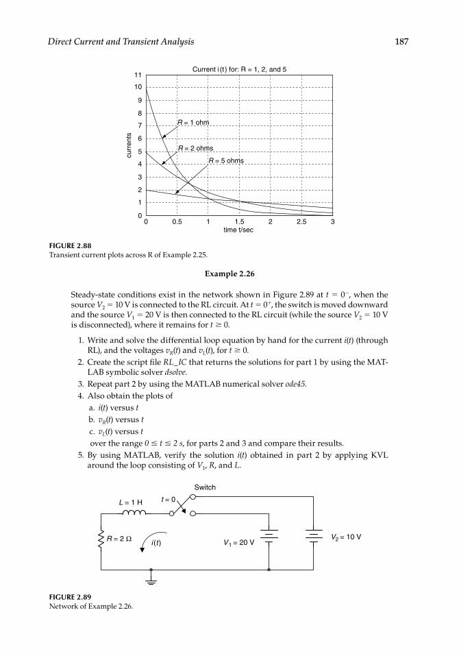
Direct Current and Transient Analysis 187
Example 2.26
Steady-state conditions exist in the network shown in Figure 2.89 at t = 0−, when the source V2 = 10 V is connected to the RL circuit. At t = 0+, the switch is moved downward and the source V1 = 20 V is then connected to the RL circuit (while the source V2 = 10 V is disconnected), where it remains for t ≥ 0.
1. Write and solve the differential loop equation by hand for the current i(t) (through RL), and the voltages vR(t) and vL(t), for t ≥ 0.
2. Create the script fi le RL_IC that returns the solutions for part 1 by using the MAT-LAB symbolic solver dsolve.
3. Repeat part 2 by using the MATLAB numerical solver ode45. 4. Also obtain the plots of
a. i(t) versus t b. vR(t) versus t c. vL(t) versus t
over the range 0 ≤ t ≤ 2 s, for parts 2 and 3 and compare their results. 5. By using MATLAB, verify the solution i(t) obtained in part 2 by applying KVL
around the loop consisting of V1, R, and L.
FIGURE 2.88Transient current plots across R of Example 2.25.
Current i (t ) for: R = 1, 2, and 511
10
9
8
7
6
curr
ents
5
4
3
2
1
00 0.5 1 1.5
time t/sec2 2.5 3
R = 1 ohm
R = 2 ohms
R = 5 ohms
FIGURE 2.89Network of Example 2.26.
V2 = 10 VR = 2 Ω
Switch
L = 1 H
V1 = 20 Vi (t )
t = 0
CRC_47760_CH002.indd 187CRC_47760_CH002.indd 187 7/23/2008 1:38:57 PM7/23/2008 1:38:57 PM

188 Practical MATLAB® Applications for Engineers
ANALYTICAL Solution
The loop differential equation is given by
V
di tdt
i t t1 20 2 0 V for( )
( )
with
A and Ai i( ) ( )0
102
5202
10
Assuming a solution for i(t) of the form i(t) = A + Be−t/τ, where τ = L/R = 0.5 s, and by using the initial and fi nal current conditions, the constants A and B can be evaluated. By following this process the current is then i(t) = 10 − 5e−2t A, and the corresponding voltages are vR(t) = 20 − 10e−2t V and vL(t) = 10e−2t V, for t ≥ 0.
MATLAB Solution% Script file: RC _ ICsyms t;% symbolic solutionit _ 1 = dsolve(‘Dy+2*y=20’,’y(0)=5’,’t’);disp(‘*****************************************’);
figure(1)subplot(3,1,1);ezplot (it _ 1,[0 2]);ylabel(‘i(t) in amps’);title(‘plots of: [i(t), vr(t) and vL(t)] vs t’);subplot(3,1,2);vtr _ 1 = it _ 1*2;ezplot(vtr _ 1,[0 2]);ylabel(‘vr(t)’);title(‘ ‘);subplot (3,1,3);vl _ 1 = 20-vtr _ 1;ezplot (vl _ 1,[0 2]);ylabel(‘vL(t)’);title(‘ ‘);xlabel (‘time in sec.’);disp(‘**********R E S U L T S ****************’);disp(‘*****************************************’);disp(‘The i(t) for t >0 is:’);it _ 1disp(‘The voltage across R=2 ohms is :’)vtr _ 1disp(‘The voltage across L=1 henry is :’)vl _ 1disp(‘********Verify solution******************’);echo on disp(‘******************************************’)verify = diff(it _ 1,t)+2*it _ 1echo off% numerical solution clear;% solution using ode45t0 = 0;R=2;tf = 2;ts = [t0 tf];i0 = 5; % initil cond.t =linspace(0,2,100);[t,it] = ode45(‘f’,ts,i0);
CRC_47760_CH002.indd 188CRC_47760_CH002.indd 188 7/23/2008 1:38:57 PM7/23/2008 1:38:57 PM

Direct Current and Transient Analysis 189
figure(2)subplot(3,1,1)plot(t,it)title(‘plots of [i(t), vr(t), and vL(t)] vs t’)ylabel(‘i(t) in amps’)subplot(3,1,2)vr=R*it’;plot(t,vr);ylabel(‘vr(t) in volts’);subplot(3,1,3)vl=20*ones(1,45)-vr;plot(t,vl);ylabel(‘vL(t) in volts ‘);xlabel(‘time in sec’)
function didt=f(t,i)didt=20-2*i;
The script fi le RC_IC is executed, and the results and plots are shown in Figures 2.90 and 2.91.>> RC _ IC
*************************************************R E S U L T S *****************************************************The i(t) for t >0 is:it _ 1 = 10-5*exp(-2*t)The voltage across R=2 ohms is : vtr _ 1 = 20-10*exp(-2*t)The voltage across L=1 henry is : vl _ 1 = 10*exp(-2*t)********Verify solution************verify = diff(it _ 1,t)+2*it _ 1verify = 20*************************************
FIGURE 2.90Plots of symbolic transient solutions of Example 2.26.
21.81.61.41.21t
t
0.80.60.40.20
6
8
10plots of: [i(t), vr(t), and vL(t)] versus t
i(t)
in a
mps
vr(t
)vL
(t)
21.81.61.41.210.80.60.40.2010
15
20
21.81.61.41.21
time in sec
0.80.60.40.200
5
10
CRC_47760_CH002.indd 189CRC_47760_CH002.indd 189 7/23/2008 1:38:58 PM7/23/2008 1:38:58 PM

190 Practical MATLAB® Applications for Engineers
Note that the symbolic results shown in Figure 2.90 fully agree with the numerical results shown in Figure 2.91.
Example 2.27
Steady-state conditions exist in the network shown in Figure 2.92 at t = 0−, when the V1 = 10 V source is connected to the RC circuit. At t = 0+, the switch moves downward, and the V2 = 20 V source is connected to the RC circuit (while the source V1 = 10 V is disconnected), for t ≥ 0.
1. Write and solve the loop differential equation by hand, for the current i(t) (through RC) and the voltages vR(t) and vC(t), for t ≥ 0.
2. Create the script fi le RC_IC that returns the solutions for part 1 using the MATLAB symbolic solver dsolve.
3. Repeat part 1 by using the MATLAB numerical solver ode45. 4. Also, obtain the plots of
a. i(t) versus t b. vR(t) versus t c. vc(t) versus t
over the range 0 ≤ t ≤ 2 s, for parts 2 and 3.
FIGURE 2.91Plots of numerical transient solutions of Example 2.26.
21.81.61.41.210.80.60.40.20
6
4
8
10plots of [i(t), vr(t), and vL(t)] versus t
i(t)
in a
mps
vr(t
) in
vol
tsvL
(t)
in v
olts
21.81.61.41.210.80.60.40.2010
15
10
21.81.61.41.210.8
time in sec
0.60.40.200
5
10
CRC_47760_CH002.indd 190CRC_47760_CH002.indd 190 7/23/2008 1:38:58 PM7/23/2008 1:38:58 PM

Direct Current and Transient Analysis 191
5. By using MATLAB, verify the solution vC(t) obtained in part 2 by applying KVL around the active loop for t > 0.
6. Compare the results of part 1 with the results of part 2 and 3.
ANALYTICAL Solution
The loop differential equation for t ≥ 0 is given by
20 2 v t i tC( ) ( ) for 0t
with νC(0) = 10 V and νC(∞) = 20 V.
Replacing i(t) = C dvc(t) _____
dt in the preceding differential equation yields
2 20
dv tdt
v tCC
( )( )
Then assuming a solution for vC(t) of the form vC(t) = A + B e−t/τ, where τ = C * R = 2 s, and knowing the initial and fi nal voltage values across C, the constants A and B can be evaluated. By following this process the voltage across C is given by vC(t) = 20 − 10 e−0.5t V, the voltage across R is vR(t) = 10 e−0.5t V, and the current is i(t) = 5e−0.5t A.
MATLAB Solution% Script file: RC _ ICsyms t;% symbolic solutionvct=dsolve(‘2*Dy+y=20’,’y(0)=10’,’t’);disp(‘*******************************************’);disp(‘***********R E S U L T S *****************’);disp(‘*******************************************’);
FIGURE 2.92Network of Example 2.27.
V1 = 10 V
Switch moves down at t = 0
+
−
C1= 1 F
R = 2 Ω
V2 = 20 V
i (t )
CRC_47760_CH002.indd 191CRC_47760_CH002.indd 191 7/23/2008 1:38:58 PM7/23/2008 1:38:58 PM

192 Practical MATLAB® Applications for Engineers
figure(1)subplot(3,1,1);ezplot(vct,[0 2]);ylabel(‘vc(t) in volts’);title(‘plots of: [vc(t), vr(t) and i(t)] vs t’);subplot(3,1,2);vrt=20-vctezplot(vrt,[0 2]);ylabel(‘vr(t)in volts’);title(‘ ‘);subplot(3,1,3);it = vrt/2;ezplot(it,[0 2]);ylabel(‘it(t)in amps’);title(‘ ‘);xlabel(‘time in sec.’);disp(‘The voltage across C, vc(t) for t >0 is:’);vctdisp(‘The voltage across R=2 ohms is :’)vrtdisp(‘The current i(t) is :’)itdisp(‘********Verify solution*******************’);echo onverify = 2*diff(vct,t)+vctdisp(‘*******************************************’)% numerical solutionclear;% solution using ode45t0 = 0;R = 2;tf = 2;ts = [t0 tf];v0 = 10; % initial conditiont = linspace(0,2,100);[t,vt] = ode45(‘f’,ts,v0);
figure(2)subplot(3,1,1)plot(t,vt)title(‘plots of [vc(t), vr(t), and i(t)] vs t’)ylabel(‘vc(t) in volts’)subplot(3,1,2)vr = 20*ones(1,41)-vt’;plot(t,vr)ylabel(‘vr(t) in volts’)subplot(3,1,3)it=vr./R;plot(t,it)ylabel(‘i(t) in volts ‘)xlabel(‘time in sec’)
function dvtdt=f(t,vt)dvtdt=10-0.5*vt;
CRC_47760_CH002.indd 192CRC_47760_CH002.indd 192 7/23/2008 1:38:58 PM7/23/2008 1:38:58 PM

Direct Current and Transient Analysis 193
The script fi le RC_IC is executed, and the results and plots are shown as follows(Figures 2.93 and 2.94):
>> RC _ IC
**************************************************** R E S U L T S **********************************************************The voltage across C, vc(t) for t >0 is: vct = 20-10*exp(-1/2*t)The voltage across R=2 ohms is : vrt = 10*exp(-1/2*t)The current i(t) is : it = 5*exp(-1/2*t)********Verify solution******************verify = 2*diff(vct,t)+vctverify = 20******************************************
FIGURE 2.93Plots of symbolic transient solutions of Example 2.27.
21.81.61.41.210.80.60.40.20
12
10
14
16
plots of: [vc(t), vr(t), and i(t)] versus t
21.81.61.41.21t
t
0.80.60.40.20
6
4
8
10
21.81.61.41.21time in sec
0.80.60.40.20
3
2
4
5
vr(t
) in
vol
tsvc
(t)
in v
olts
it(t)
in a
mps
CRC_47760_CH002.indd 193CRC_47760_CH002.indd 193 7/23/2008 1:38:58 PM7/23/2008 1:38:58 PM

194 Practical MATLAB® Applications for Engineers
Note that the analytical solution fully agrees with the symbolic and numerical solutions shown in Figures 2.93 and 2.94.
Example 2.28
Steady-state conditions exist in the network shown in Figure 2.95 at t = 0−, when the V0 = 10 V source is connected to the RCL circuit. At t = 0+, the switch moves downward, and the source V0 = 10 V and resistor R are disconnected from the LC structure, where it remains for t ≥ 0.
Write the second-order loop differential equation in terms of the current i(t), solve and plot i(t) using MATLAB over the range 0 ≤ t ≤ 1 s, and verify that the LC network is an ideal oscillator.
ANALYTICAL Solution
CL or
CLd i tdt
i td i tdt
i t t2
2
2
20
10 0
( )( )
( )( ) for
d i tdt
i t2
2144 0
( )( )
FIGURE 2.94Plots of numerical transient solutions of Example 2.27.
21.81.61.41.210.80.60.40.2010
15
20
plots of: [vc(t), vr(t), and i(t)] versus t
21.81.61.41.210.80.60.40.20
5
0
10
21.81.61.41.21
time in sec
0.80.60.40.20
2
0
4
6
i(t)
in v
olts
vr(t
) in
vol
tsvc
(t)
in v
olts
CRC_47760_CH002.indd 194CRC_47760_CH002.indd 194 7/23/2008 1:38:59 PM7/23/2008 1:38:59 PM

Direct Current and Transient Analysis 195
with the boundary conditions given by
L
di tdt
vt C( )
( ) 0 0 10 V
or
di tdt
it( )
( ) 0 40 0 0 V and A
Note that L
di tdt C
i t t( )
( ) 1
0 0∫ for satisfying KVL
MATLAB Solution>> current _ it = dsolve(‘D2y+144*y=0’,’y(0)=0,Dy(0)=40’,’t’)
current _ it = 10/3*sin(12*t)
>> ezplot(it,[0 1]) % the plot is shown in Figure 2.96>> xlabel(‘time t in sec’)>> ylabel(‘i(t) in amps’)>> title(‘i(t) vs t’)
FIGURE 2.95Network of Example 2.28.
FIGURE 2.96Plot of i(t) of Example 2.28.
0 0.1 0.2 0.3 0.4 0.5 0.6 0.7 0.8 0.9 1−4
−3
−2
−1
0
1
2
3
4
time t in sec
i(t) versus t
i(t)
in a
mps
V0 = 10 V
Switch moves down at t = 0
++
−−
C1 = 1/36 F
R = 2 Ω
i (t )
L = 1/4 H
CRC_47760_CH002.indd 195CRC_47760_CH002.indd 195 7/23/2008 1:38:59 PM7/23/2008 1:38:59 PM

196 Practical MATLAB® Applications for Engineers
Note that the network shown in Figure 2.95 is an ideal circuit (since there is no resis-tance, R = 0 in the LC loop for t ≥ 0), and the solution clearly indicates that the current shows an oscillator behavior with W = 12 rad/s = 1 _____
√ ___
LC and T = π __ 6 s.
Example 2.29
Steady-state conditions exist in the network shown in Figure 2.97 at t = 0−, when the V1 = 120 V source is connected to the RCL parallel circuit. At t = 0+, the switch moves downward, and the source V1 = 120 V and resistor R = 10 Ω are disconnected from the parallel (RLC) structure.
Analyze the transient response (t > 0) of the source-free parallel RLC circuit, for each of the following values of R, R = 3, 9, and 72 Ω.
1. Determine the analytical response vC(t) for each value of R, for t ≥ 0 2. Create the script fi le transient_RLC_parallel that returns the MATLAB solutions of
part 1 and its corresponding voltage plots 3. Compare the MATLAB solutions of part 2 with the analytical solutions of part 1
FIGURE 2.97Network of Example 2.29.
L = 9 H
R = 10 Ω
R = 3,9 and 72 Ω
V1 = 120 V
Switch moves down at t = 0
C = 1/36 F
ANALYTICAL Solution
From the circuit diagram of Figure 2.97 for t ≤ 0, the initial conditions are vC(0) = 0 and iL(0) = 120/10 = 12 A, and
C
dv tdt
i t i i iCt C C L R
( )( ) ( ) ( ) ( ) 0 0 0 0 0
then
dv t
dtiC
t C( )
( ) ( ) 0 36 0 36 12 0 432 V/s
Recall that the node equation is
d v t
dtdv t
dtv t tC C
C
2
2
1 10 0
( ) ( )( )
RC CLfor
For R = 3 Ω, the resonant frequency is
w0
12
LC rad/s
CRC_47760_CH002.indd 196CRC_47760_CH002.indd 196 7/23/2008 1:38:59 PM7/23/2008 1:38:59 PM

Direct Current and Transient Analysis 197
The neper frequency is
12
6RC
Hz
The complex frequencies are s1 and s2, given by
s w1 22
02
,
then 0 > √ _______
α2 − w 0 2 and is clearly the overdamped case.
Then the solution vC(t) is of the form vC(t) = A1e−s1t + A2e−s2t
For R = 9 Ω, the resonant frequency is
w0
12
LC rad/s
The neper frequency is
12
2RC
Hz
Then s1 and s2 are negative and repeated frequencies, which are given by
s w1 22
02
,
Since 0 = √ _______
α2 − w 0 2 , the case is critical damped.
Then the solution vC(t) is of the form vC(t) = A1e−αt + A2 t e−αt
For R = 72 Ω, the resonant frequency is
w0
12
LC rad s/
The neper frequency is
12
14RC
Hz
The complex frequencies s1 and s2 are given by s1,2 = −α ± j √ _______
w 0 2 − α2 (complex conju-
gate), and is clearly the underdamped case. Then the solution vC (t) is of the form
v t e A w t A w ttd d( ) [ cos( ) sin( )]
1 2
where wd = √ _______
w 0 2 − α2 .
Let us use MATLAB to obtain and plot the solutions just presented, and compare them with the analytical results.
CRC_47760_CH002.indd 197CRC_47760_CH002.indd 197 7/23/2008 1:38:59 PM7/23/2008 1:38:59 PM

198 Practical MATLAB® Applications for Engineers
MATLAB Solution% Script file : transient _ RLC _ parallel% source free RLC parallel circuit analysisdisp(‘***************************************’)disp(‘*******R E S U L T S*******************’)disp(‘Source free parallel RLC circuit’)disp(‘***************************************’)disp(‘Solution of diff. equation for R=3 ohms’)overdamped = dsolve(‘(1/36)*D2y+(1/3)*Dy+(1/9)*y=0’,’y(0) = 0’,’Dy(0)= 32’,’t’)
figure(1)ezplot(overdamped)xlabel(‘time (sec)’)ylabel(‘voltage(volts)’)title(‘v(t) vs t (overdamped case; R=3 ohms)’)axis([0 3 0 40]);disp(‘***************************************’)
figure(2)disp(‘Solution of diff. equation for R=9 ohms’)criticaldamped = dsolve(‘(1/36)*D2y+(1/9)*Dy+(1/9)*y=0’,’y(0)=0’,’Dy(0)=432’,’t’)simple _ crit=simple(criticaldamped);ezplot(criticaldamped)xlabel(‘time (sec)’)ylabel(‘voltage(volts)’)title(‘v(t) vs t (criticaldamped case; R=9 ohms)’)axis([0 4 0 90]);disp(‘***************************************’)disp(‘Solution of diff. equation for R=72 ohms’)underdamped = dsolve(‘(1/36)*D2y+(1/72)*Dy+(1/9)*y=0’,’y(0)=0’,’Dy(0)=432’,’t’)
figure(3)ezplot(underdamped)xlabel(‘time (sec)’); ylabel(‘voltage(volts)’)title(‘v(t) vs t (underdamped case; R=72 ohms)’)axis([0 6 -150 200]);disp(‘****************************************’)
The script fi le transient_RLC_parallel is executed, and the results and plots (Figures 2.98 through 2.100) are as follows:
>> transient _ RLC _ parallel
**********************************************R E S U L T S*******************Source free parallel RLC circuit ***************************************Solution of diff. equation for R=3 ohmsoverdamped = 27*2 (1/2)*exp(2*(-3+2*2 (1/2))*t)-27*2 (1/2)*exp(-2*(3+2*2 (1/2))*t)***************************************Solution of diff. equation for R=9 ohmscriticaldamped = 432*exp(-2*t)*t***************************************Solution of diff. equation for R=72 ohmsunderdamped = 576/7*7 (1/2)*exp(-1/4*t)*sin(3/4*7 (1/2)*t)****************************************
CRC_47760_CH002.indd 198CRC_47760_CH002.indd 198 7/23/2008 1:39:00 PM7/23/2008 1:39:00 PM

Direct Current and Transient Analysis 199
FIGURE 2.98Transient overdamped plot (t > 0) of the source-free parallel RLC of Example 2.29.
0 0.5 1 1.5 2 2.5 30
5
10
15
20
25
30
35
40
time (sec)
v(t) versus t (overdamped case; R = 3 ohms)
volta
ge (
volts
)
FIGURE 2.99Transient critical damped plot (t > 0) of the source-free parallel RLC of Example 2.29.
0 0.5 1 1.5 2 2.5 3 3.5 40
10
20
30
40
50
60
70
80
90
time (sec)
v(t) versus t (critical damped case; R = 9 ohms)
volta
ge (
volts
)
FIGURE 2.100Transient underdamped plot (t > 0) of the source-free parallel RLC of Example 2.29.
0 1 2 3 4 5 6−150
−100
−50
0
50
100
150
200
time (sec)
v(t) versus t (underdamped case; R = 72 ohms)
volta
ge (
volts
)
CRC_47760_CH002.indd 199CRC_47760_CH002.indd 199 7/23/2008 1:39:00 PM7/23/2008 1:39:00 PM

200 Practical MATLAB® Applications for Engineers
Observe that by changing the value of R (R = 3, 9, and 72 Ω), the three solutions for the second-order differential equation—over, critical, and underdamped—are obtained. Observe that the analytical solutions completely agree with the MATLAB solutions.
Example 2.30
Steady-state conditions exist in the network shown in Figure 2.101, at t = 0−, when the V0 = 90 V source is connected to the RCL circuit. At t = 0+, the switch opens (moves upward) and the source V0 = 90 V is disconnected from the RLC structure.
Analyze the transient response (t > 0) of the source-free series RLC circuit for the following values of R, R = 75, 36, and 3 Ω.
1. Determine the analytical response iR(t) for each value of R, for t ≥ 0 2. Create the script fi le transient_RLC_series that returns the MATLAB solutions of
part 1, and its plots 3. Compare the MATLAB solutions of part 2 with the analytical solutions of part 1
FIGURE 2.101Network of Example 2.30.
C = 1/36 F
V0 = 90 V
L = 9 H
R = 75, 36, and 3 Ω Switch opens at t = 0
ANALYTICAL Solution
For t ≤ 0−, the initial conditions are vC(0) = 90 V and iL(0) = 0 A.
L
di tdt
Ri vt C( )
( ) ( ) 0 0 0
then
di tdt
v Ri tL
vLt
C L C( ) ( ) ( ) ( )/s 0
0 0 909
10
A
Recall that the loop differential equation is
d i tdt
RL
di tdt
i t t2
2
10 0
( ) ( )( )
CLfor
CRC_47760_CH002.indd 200CRC_47760_CH002.indd 200 7/23/2008 1:39:00 PM7/23/2008 1:39:00 PM

Direct Current and Transient Analysis 201
For R = 75 Ω, the resonant frequency is
w0
12
LC rad/s
The neper frequency is
RL2
7518
4 1667. Hz
The frequencies s1 and s2 are
s w1 22
02
,
then
0 202 w
and the solution i(t) is the overdamped case given by i(t) = A1e−s1t + A2e−s2t.For R = 36 Ω, the resonant frequency is
w0
12
LC rad/s
The neper frequency is
RL2
3618
2 Hz
and s1 and s2 are repeated, given by
s w1 22
02
,
then
0 202 w
and the solution i(t) is the critical-damped case given by i(t) = A1e−αt + A2te−αt.For R = 3 Ω, the resonant frequency is
w0
12
LC rad/s
The neper frequency is
RL2
318
16
0 1667. Hz
and the complex frequencies are s1 and s2 given by s1,2 = −α ± j √ _______
w 0 2 − α2 , clearly the
underdamped case.Then the solution i(t) is of the form
i t e A w t A w ttd d( ) [ cos( ) sin( )]
1 2
where wd = √ _______
w o 2 − α2 .
CRC_47760_CH002.indd 201CRC_47760_CH002.indd 201 7/23/2008 1:39:00 PM7/23/2008 1:39:00 PM

202 Practical MATLAB® Applications for Engineers
MATLAB Solution% Script file : transient _ RLC _ series % source free RLC series circuit analysisdisp(‘****************************************’)disp(‘************R E S U L T S**************’)disp(‘*****Source free series RLC circuit***’)disp(‘****************************************’)disp(‘Solution of diff. equation for R=75 ohms’)overdamped = dsolve(‘D2y+(75/9)*Dy+4*y=0’,’y(0)=0’, ‘Dy(0)=10’,’t’)
figure(1)ezplot (overdamped,[0 5])xlabel (‘time (sec)’)ylabel (‘current i(t) in amps’)title (‘i(t) vs t (overdamped case; R=75 ohms)’)disp (‘***************************************’)
figure(2)disp(‘Solution of diff. equation for R=36 ohms’)criticaldamped = dsolve(‘D2y+(36/9)*Dy+4*y=0’,’y(0)=0’,’Dy(0)=10’,’t’)ezplot(criticaldamped,[0 6])xlabel(‘time (sec)’); ylabel(‘current i(t) in amps’)title(‘i(t) vs t (criticaldamped case; R=36 ohms)’)disp(‘*************************************************************’)disp(‘Solution of diff. equation for R=3 ohms’)underdamped = dsolve(‘D2y+(3/9)*Dy+4*y=0’,’y(0)=0’,’Dy(0)=10)
figure(3)ezplot (underdamped)xlabel (‘time (sec)’)ylabel (‘current i(t) in amps’)title (‘i(t) vs t (underdamped case; R=3 ohms)’)disp(‘**************************************************************’)
The script fi le transient_RLC_series is executed, and the results and plots (Figures 2.102 through 2.104) are as follows:
>> transient _ RLC _ series *********************************************************R E S U L T S******************************* ***Source free series RLC circuit *****************************************************************************Solution of diff. equation for R=75 ohmsoverdamped = 30/481*481 (1/2)*exp(1/6*(-25+481 (1/2))*t)- 30/481*481 (1/2)*exp(- 1/6*(25+481 (1/2))*t)**************************************************************************Solution of diff. equation for R=36 ohmscriticaldamped = 10*exp(-2*t)*t**************************************************************************Solution of diff. equation for R=3 ohmsunderdamped = 60/143*143 (1/2)*exp(-1/6*t)*sin(1/6*143 (1/2)*t)**************************************************************************
CRC_47760_CH002.indd 202CRC_47760_CH002.indd 202 7/23/2008 1:39:01 PM7/23/2008 1:39:01 PM

Direct Current and Transient Analysis 203
FIGURE 2.102Transient overdamped plot (t > 0) of the source-free series RLC of Example 2.30.
0 0.5 1 1.5 2 2.5 3 3.5 4 4.5 5
0
0.2
0.4
0.6
0.8
1
time (sec)
i(t) versus t (overdamped case; R = 75 ohms)
curr
ent i
(t)
in a
mps
FIGURE 2.103Transient critical damped plot (t > 0) of the source-free series RLC of Example 2.30.
0 1 2 3 4 5 6
00.20.40.60.8
11.21.41.61.8
2
time (sec)
i(t) versus t (critical damped case; R = 36 ohms)
curr
ent i
(t)
in a
mps
FIGURE 2.104Transient underdamped plot (t > 0) of the source-free series RLC of Example 2.30.
−6 −4 −2 0 2 4 6
−10
−5
0
5
10
time (sec)
i(t) versus t (underdamped case; R = 3 ohms)
curr
ent i
(t)
in a
mps
CRC_47760_CH002.indd 203CRC_47760_CH002.indd 203 7/23/2008 1:39:01 PM7/23/2008 1:39:01 PM

204 Practical MATLAB® Applications for Engineers
Observe that by changing the value of R (R = 75, 36, and 3 Ω), the three solutions for the second-order differential equation—over, critical, and underdamped cases—are obtained. Also observe that the analytical solutions completely agree with the MATLAB solutions.
Example 2.31
Steady-state conditions exist in the circuit of Figure 2.105 for t ≤ 0, while the voltage source V1 = 6 V is connected to the network. At t = 0+, the switch moves downward disconnecting the source while connecting R1 to the rest of the circuit.
1. Obtain analytically the loop differential equation set and the initial conditions 2. Using the MATLAB symbolic solver, create the script fi le transient_2loops that
returns the transient currents for each loop, and their respective plots, for t ≥ 0 3. Also obtain simplify and pretty expressions for each of the transient loop currents of
part 2
FIGURE 2.105Network of Example 2.31.
V1 = 6 VR3 = 6 Ω
R2 = 3 Ω
R1 = 4 Ω
Switch moves down at t = 0
+ −
+
−
L1 = 1 H
i2(t )i1(t )
L2 = 2 H
+
−+
−
ANALYTICAL Solution
The conditions at t = 0 are i1(0) = 3 A and i2(0) = 1 A. Applying KVL to the two-mesh network of Figure 2.105, for t ≥ 0, results in the following set of simultaneous differen-tial equations:
( ) ( )
( )( )R R i t L
di tdi
R i t1 2 1 11
2 2 0
R i t R R i t L
di tdi2 1 3 2 2 22 0( ) ( ) ( )( )
Replacing the elements by their values yields the following set of differential equations:
7 3 01
12i t
di tdi
i t( )( )
( )
CRC_47760_CH002.indd 204CRC_47760_CH002.indd 204 7/23/2008 1:39:01 PM7/23/2008 1:39:01 PM

Direct Current and Transient Analysis 205
or
di t
dii t i t11 27 3
( )( ) ( )
and
3 9 2 01 2
2i t i tdi t
di( ) ( )
( )
or
2 3 92
1 2di t
dti t i t
( )( ) ( )
MATLAB Solution% Script file : transient _ 2loops% transient solutions for two loop networkdisp(‘****************************************’)disp(‘*******R E S U L T S*******************’)disp(‘****************************************’)disp(‘Solution of the two diff. loop equations for t>0 ’)[y1 y2] = dsolve(‘Dy1=-7*y1+3*y2,2*Dy2=3*y1- 9*y2’,’y1(0)=3’,’y2(0)=2’,’t’);
figure(1)ezplot (y1,[0 3])axis([0 1.5 0 3.5])xlabel (‘time (sec)’)ylabel (‘current i1(t) in amps’)title (‘i1(t) vs t ’)
figure(2)ezplot(y2,[0 3])axis([0 1.5 0 2.3])xlabel(‘time (sec)’)ylabel(‘current i2(t) in amps’)title(‘i2(t) vs t ’)disp(‘***************************************’)disp(‘The currents i1(t) and i2(t), in amps are :’)[y1 y2]’disp(‘***************************************’)disp(‘The simplify solution for i1(t) is:’)simplify(y1)disp(‘***************************************’)disp(‘The simplify solution for i2(t) is :’)simplify(y2)disp(‘***************************************’)disp(‘The pretty solution for i1(t) is :’)pretty(y1)disp(‘***************************************’)disp(‘The pretty solution for i2(t) is :’)pretty(y2)disp(‘***************************************’)
CRC_47760_CH002.indd 205CRC_47760_CH002.indd 205 7/23/2008 1:39:01 PM7/23/2008 1:39:01 PM

206 Practical MATLAB® Applications for Engineers
figure(3)ezplot(y1)hold onezplot(y2)xlabel(‘time (sec)’)axis([0 1.0 0 3.5])ylabel(‘currents [i1(t)&i2(t)] in amps’)title(‘i1(t) & i2(t) vs t ‘)
The script fi le transient_2loops is executed, and the results and plots (Figures 2.106 through 2.108) are as follows:
>> transient _ 2loops
***********************************************************R E S U L T S***********************************************************************************Solution of the two diff. loop equations for t>0 ****************************************************The currents i1(t) and i2(t), in amps are :ans =[ conj(-9/194*97 (1/2)*exp(-1/4*(23+97 (1/2))*t)+9/194*97 (1/2)*exp(1/4*(-23+97 (1/2))*t)+3/2*exp(1/4*(-23+97 (1/2))*t)+3/2*exp(-1/4*(23+97 (1/2))*t))][ conj(exp(1/4*(-23+97 (1/2))*t)-14/97*97 (1/2)*exp(-1/4*(23+97^ (1/2))*t)+14/97*97 (1/2)*exp(1/4*(-23+97 (1/2))*t)+exp(-1/4*(23+97 (1/2))*t))]*************************************************************The simplify solution for i1(t) is:ans = -9/194*97 (1/2)*exp(-1/4*(23+97 (1/2))*t)+9/194*97 (1/2)*exp(1/4*(-23+97^ (1/2))*t)+3/2*exp(1/4*(-23+97 (1/2))*t)+3/2*exp(-1/4*(23+97 (1/2))*t)**************************************************************************The simplify solution for i2(t) is :ans =exp(1/4*(-23+97 (1/2))*t)-14/97*97 (1/2)*exp(-1/4*(23+97 (1/2))*t)+14/97*97^ (1/2)*exp(1/4*(-23+97 (1/2))*t)+exp(-1/4*(23+97 (1/2))*t) ************************************************************************** The pretty solution for i1(t) is : 1/2 1/2 - 9/194 97 exp(- 1/4 (23 + 97 ) t) 1/2 1/2 1/2 + 9/194 97 exp(1/4 (-23 + 97 ) t) + 3/2 exp(1/4 (-23 + 97 ) t) 1/2 + 3/2 exp(- 1/4 (23 + 97 ) t)************************************************************************** The pretty solution for i2(t) is : 1/2 1/2 1/2 exp(1/4 (-23 + 97 ) t) - 14/97 exp(- 1/4 (23 + 97 ) t) 1/2 1/2 1/2 + 14/19 97 exp(1/4 (-23 + 97 ) t) + exp(- 1/4 (23 + 97 ) t)**************************************************************************
CRC_47760_CH002.indd 206CRC_47760_CH002.indd 206 7/23/2008 1:39:02 PM7/23/2008 1:39:02 PM

Direct Current and Transient Analysis 207
FIGURE 2.106Plot of i1(t) of Example 2.31.
0 0.5 1 1.50
0.5
1
1.5
2
2.5
3
3.5
time (sec)
i1(t) versus t
curr
ent i
1(t)
in a
mps
FIGURE 2.107Plot of i2(t) of Example 2.31.
0 0.5 1 1.50
0.5
1
1.5
2
time (sec)
i2(t) versus t
curr
ent i
2(t)
in a
mps
CRC_47760_CH002.indd 207CRC_47760_CH002.indd 207 7/23/2008 1:39:02 PM7/23/2008 1:39:02 PM

208 Practical MATLAB® Applications for Engineers
2.5 Application Problems
P.2.1 Create conversion tables and graphs for the fi rst 21 integer values (from 0 to 20) for the following:a. British thermal units to Joulesb. Joules to foot-pound forcec. Newton to pound-forced. Inches to centimetere. Horsepower to wattsf. Foot to meterg. Joules to caloriesh. Horsepower to foot-pound force per secondi. Kilowatt per hour to Joulesj. Electrons to coulombs
FIGURE 2.108Plots of i1(t) and i2(t) of Example 2.31.
0 0.1 0.2 0.3 0.4 0.5 0.6 0.7 0.8 0.9 10
0.5
1
1.5
2
2.5
3
3.5
time (sec)
i1(t) and i2(t) versus tcu
rren
ts [i
1(t)
and
i2(t
)] in
am
ps
i2(t)
i1(t)
CRC_47760_CH002.indd 208CRC_47760_CH002.indd 208 7/23/2008 1:39:02 PM7/23/2008 1:39:02 PM
Direct Current and Transient Analysis 209
The following relations may be of help:1 Btu = 1055 J = 778.2 ft · lbf
1 J = 0.737 ft · lbf
1 N = 0.225 lbf
1 in. = 2.54 cm1 Hp = 746 W1 ft = 0.3048 m1 Btu = 252 Cal1 Hp = 550 ft ∙ lbf/s = 33,000 ft ∙ lbf/min = 0.07067 Btu/s1 kW/h = 3.6(106) J = 3.414 Btu/h1 Cal = 3.088 ft ∙ lbf
1 C = 6.24 * 1018 electronsP.2.2 Two electric charges given by Q1 = +500 µC and Q2 = −600 µC experience a force of
1500 N. Determine the distance separating the charges and the direction of the force (attraction or repulsion).
P.2.3 An electric current I consists of 25 * 1016 electrons/s. Express I in amperes (A), mil-liampere (mA), and microampere (µA).
P.2.4 An energy E of 650 J is required to move 12 C from point A to point B. Determine the potential difference between the points (A and B).
P.2.5 Obtain tables and plots of the force of attraction versus the separation (force versus distance) of two charges Q1 = +1.500 µC and Q2 = −600 µC, where the separation distance r is over the range 0.5 m ≤ r ≤ 5 m, in intervals of 0.25 m, where the vari-ables are evaluated using the following units:a. Newtons versus metersb. Pound force versus inchesc. Newtons versus footd. Pound force versus centimeter
P.2.6 The current through a 2.7 kΩ resistor R is 3 mA. Determine the current direction and the polarity of the voltage VR across the resistor.
P.2.7 A light bulb is rated 100 W at 120 V. Find the current through the bulb and calculate its resistance.
P.2.8 If the cost of electrical energy is $0.09 kW/h, what would be the cost of using a 100 W bulb during the following time periods?a. One dayb. One weekc. One monthd. One year
P.2.9 Convert the MATLAB programs of Examples 2.2 and 2.3 into script fi les.P.2.10 Determine the equivalent resistances of each of the networks shown in Figure 2.109
by hand and by using MATLAB.
•••••••••••
CRC_47760_CH002.indd 209CRC_47760_CH002.indd 209 7/23/2008 1:39:02 PM7/23/2008 1:39:02 PM

210 Practical MATLAB® Applications for Engineers
P.2.11 The potentiometer R5 of the circuit diagram of Figure 2.110 varies over the range 0 ≤ R5 ≤ 100 Ω in linear increments of 5 Ω. Write a MATLAB program that returns the following plots:a. R5 versus I1
b. R5 versus I2
c. R5 versus I3
d. R5 versus I4
e. R5 versus I5
P.2.12 Repeat P.2.11 for the following cases:a. R5 versus VR1
b. R5 versus VR3
c. VR1 versus VR5
d. VR3 versus I5
P.2.13 For the circuit diagram shown in Figure 2.110, write a program that returns the fol-lowing plots:a. R5 versus power of R3
b. R5 versus power of (R1||R2)c. R5 versus power of (R4||R5)d. R5 versus power of (V)
P.2.14 For the circuit shown in Figure 2.110, write and run a program that returns the following plots as R5 varies over the range 0 ≤ R5 ≤ 100 Ω in linear increments of 5 Ω:a. VR3 versus VR1
FIGURE 2.109Network of P.2.10.
2
8
8
6
2 4
1
300
600
300
600
(a)
(b) (c)
10
50 200 50
300 600
CRC_47760_CH002.indd 210CRC_47760_CH002.indd 210 7/23/2008 1:39:02 PM7/23/2008 1:39:02 PM

Direct Current and Transient Analysis 211
FIGURE 2.110Network of P.2.11.
R1 = 10 Ω
R2 = 20 Ω
R3 = 30 Ω
V0 = 100 V
I2
I1
I3
I5I4
R4 = 25 ΩR5
+
−
FIGURE 2.111Network of P.2.15.
R3 = 5 Ω
I
B A
C
I1
R4 = 20 Ω R5 = 10 Ω
R2 = 5 Ω
R1 = 10 Ω
I3
I2
FIGURE 2.112Network of P.2.16.
R6 = 20 ΩR5 = 5 ΩR4 = 10 Ω
R1 = 10 Ω
R2 = 20 Ω R3 = 30 Ω
V0
I2
I5
I1
+
−
b. I5 versus I3
c. I1 versus I5
P.2.15 The current source I, shown in the circuit of Figure 2.111, varies over the range 1 mA ≤ I ≤ 0.5 A in linear increments of 10 mA.
CRC_47760_CH002.indd 211CRC_47760_CH002.indd 211 7/23/2008 1:39:03 PM7/23/2008 1:39:03 PM

212 Practical MATLAB® Applications for Engineers
Write a program that returns the following plots:a. I versus VAB
b. I versus VBC
c. I versus I1
d. I versus I3
e. I versus power (R1 R2)P.2.16 The voltage source V0 shown in Figure 2.112, varies from 10 to 100 V in steps (incre-
ments) of 5 V. Write a program that returns the following plots:a. V0 versus I1
b. V0 versus VR5
c. V0 versus I2
d. V0 versus I5
e. V0 versus power of R2
P.2.17 The diagrams shown in Figure 2.113 represent the circuit equivalent ∆-to-Y transformations.
FIGURE 2.113Network structures of P.2.17.
BA
C
A B
C
R1
R2 R3
RA RB
RC
FIGURE 2.114Network of P.2.17.
100 V
Y
X10 50
40 + − 20
30
Loop IILoop I
CRC_47760_CH002.indd 212CRC_47760_CH002.indd 212 7/23/2008 1:39:03 PM7/23/2008 1:39:03 PM

Direct Current and Transient Analysis 213
The ∆-to-Y transformation equations are
R
R RR R RA
1 2
1 2 3
*
R
R RR R RB
1 3
1 2 3
*
R
R RR R RC
2 3
1 2 3
*
Calculate the voltage VXY in the circuit shown in Figure 2.114 bya. Applying the ∆-to-Y transformation to loop I onlyb. Applying the ∆-to-Y transformation to loop II onlyc. Using loop equations (with no transformations)d. Applying Thevenin’s theorem (assuming that the load is R = 30)
FIGURE 2.115Current iC of P.2.19.
t (seconds)
50
1 mA
iC
FIGURE 2.116Voltage vL of P.2.20.
t (seconds)
0
1 V
vL
e. Using node equations (with no transformations)f. Applying Norton’s theorem (assuming that the load is R = 30) Assume that all the resistors are given in ohms.
P.2.18 From the equations for RA, RB, and RC defi ned in P.2.17, obtain expressions for R1, R2, and R3 for the Y-to-∆ transformations by hand and by using MATLAB symbolic techniques.
CRC_47760_CH002.indd 213CRC_47760_CH002.indd 213 7/23/2008 1:39:03 PM7/23/2008 1:39:03 PM

214 Practical MATLAB® Applications for Engineers
P.2.19 The current iC(t) through a capacitor C = 1 µF is shown in Figure 2.115.Write a MATLAB program that returns the following plots:
a. The voltage vC (t) versus t
b. The energy Wc(t) versus t over the range 0 ≤ t ≤ 10 sP.2.20 The voltage across the inductor L = 1 mH is shown in Figure 2.116. Write a MATLAB
program that returns the following plots:a. The current iL(t) versus tb. The energy wL(t) versus t over the range 0 ≤ t ≤ 10 s
P.2.21 The RC circuit shown in Figure 2.117 presents an initial voltage vC(0) = 0 V at the instant the switch closes at t = 0.
Write a program that returns the following plots over the range 0 ≤ t ≤ 5 s:a. Current i(t) versus t
b. Voltage vR(t) versus t
c. Voltage vC(t) versus t
d. Energy wC in Joules stored in C versus t
e. Instantaneous power in watts dissipated by R versus t
FIGURE 2.119Networks of P.2.23.
L1
V
vL1 vL2
vC1 vC2
L2 C1 C2
(b)(a)
V+−
+−
FIGURE 2.118Network of P.2.22.
Switch closes at t = 0
L = 1 mH
R = 1 kΩ
100 V
i (t )
FIGURE 2.117Network of P.2.21.
Switch closes at t = 0
R = 1 kΩ
C = 1 mF
100 V
i (t )
CRC_47760_CH002.indd 214CRC_47760_CH002.indd 214 7/23/2008 1:39:03 PM7/23/2008 1:39:03 PM

Direct Current and Transient Analysis 215
P.2.22 The RL circuit in Figure 2.118 presents an initial current i(0) = 0 A at the instant the switch closes at t = 0, where it remains indefi nitely. Write a program that returns the following plots over the range 0 ≤ t ≤ 10 s:a. [Current i(t)] versus tb. Voltage vR (t) versus tc. Voltage vL (t) versus td. [Energy wL in Joules stored in L] versus te. [Power in watts dissipated by R] versus t
P.2.23 Determine VL2 and VC2 shown in the circuits of Figure 2.119 in a tablelike format; given V = 100 V, L2 = 10 H, and C2 = 10 F for the following cases:a. L1 varies from L2/2 to 2L2 in linear steps of L2/10.b. C1 varies from C2/2 to 2C2 in linear steps of C2/10.
P.2.24 For the circuit diagrams shown in Figure 2.120a. Evaluate by hand the expressions for the current I1
b. Plot I1 as a function of L2, if L1 = 5 H and L2 varies over the range 0 ≤ L2 ≤ 15 H in steps (increments) of 0.5 H
c. Repeat part b for the case where C1 = 5 F and C2 varies over the range 0 ≤ C2 ≤ 15 F in steps (increments) of 0.5 F
FIGURE 2.120Networks of P.2.24.
L11 A 1 A
(a)
L2I1 C2C1I1
(b)
FIGURE 2.121Network of P.2.25.
V0 = 100 V
R3 = 3 Ω
R1 = 10 Ω R2 = 15 Ω
R4 = 30 Ω
I5I2I1
I3 I4C1 = 1 F
C2 = 2 F L = 1 H+−
X Y
CRC_47760_CH002.indd 215CRC_47760_CH002.indd 215 7/23/2008 1:39:04 PM7/23/2008 1:39:04 PM

216 Practical MATLAB® Applications for Engineers
P.2.25 For the circuit shown in Figure 2.121, evaluatea. I1, I2, I3, I4, and I5
b. VX, VY, and VXY
c. Power of all the resistors in watts, horsepower, and foot-pound force per second (see P.2.1)
d. The energy stored in C1, C2, and LP.2.26 The network structure shown in Figure 2.122 is called “lattice.”
Observe that the resistors, R1, R3, …, R2n−1 (ohms), placed horizontally are labeled with odd indexes, whereas the elements in the vertical positions are admittances G1, G4, …, G2n (ohms−1 or siemans), which are labeled with even indexes.
Verify the following expression:
R R
G R G R R Gn n
12 3 4 5 2 1 2
1 1 1 1 1 1
FIGURE 2.123Network of P.2.27.
2 Ω 3 Ω 1 Ω
1 Ω 3 Ω 5 Ω 7 Ω
2 Ω−13 Ω−1 4 Ω−1
2 Ω−1 4 Ω−1 6 Ω−1 8 Ω−1
(a)
(b)
R
R
FIGURE 2.122Lattice network of P.2.26.
1/R2 = G2 1/R4 = G4 1/R6 = G6 1/R2n = G2n
R7R5R3R1
R
R2n−1
CRC_47760_CH002.indd 216CRC_47760_CH002.indd 216 7/23/2008 1:39:04 PM7/23/2008 1:39:04 PM

Direct Current and Transient Analysis 217
P.2.27 For the circuits shown in Figure 2.123 evaluate R bya. Writing a MATLAB program using the standard circuit analytical techniquesb. Writing a MATLAB program that computes R by using the relation of P.2.26
given by
R R
G Rn n
i ii
n
i
n
12 2 111
1 1
∑∑ for 3 and 4
P.2.28 Draw the possible circuit diagrams for the electrical network defi ned by the follow-
ing set of mesh equations:a. 20I1 − 5I2 = 10 −5I1 + 10I2 = −7b. 10 = 6I1 − 2I2 − 3I3
−6 = −2I1 + 6I2 − 4I3
5 = −3I1 − 4I2 + 12I3
c. Using MATLAB, solve each system (a and b) that consists of the set of loop equations
P.2.29 Verify that the equivalent resistance (between terminals a and a’) of the circuit of Figure 2.124 is given by
R
R R R R R R R R R R R R RR R R R
1 2 3 4 3 4 1 2 5 1 3 2 4
1 2 3 4
* ( ) * ( ) ( )( )( )( ) ( )R R R R R1 2 3 4 5
P.2.30 Evaluate the equivalent resistance between terminals a and a’, of the circuit dia-gram shown in Figure 2.124, by applying the following techniques or procedures:a. Connect an arbitrary voltage source V across aa’, solve for the current I, and then
evaluate Raa’ = V/I
FIGURE 2.124Network of P.2.29.
I
R1
R2
R3
R4
R5
a ′a
FIGURE 2.125Network of P.2.31.
R1 R2
R2 R1
R3
a ′ a
I
CRC_47760_CH002.indd 217CRC_47760_CH002.indd 217 7/23/2008 1:39:04 PM7/23/2008 1:39:04 PM

218 Practical MATLAB® Applications for Engineers
FIGURE 2.126Network of P.2.33.
b
V = 100 V
L = 2 H
R3 = 9 Ω
R2 = 1 Ω
R1 = 1 Ω
a i3(t )
i2(t )
i1(t )
C = 2 F
+ −
FIGURE 2.127Network of P.2.34 and P.2.35.
80 Ω
3 A 30 Ω
3 Ω
6 Ω
2 Ω
4 V
10 V
60 Ω
80 V
A
B
A
B
FIGURE 2.128Network of P.2.36.
10 A
2 Ω
8 Ω3 Ω
20 V I
b. Direct evaluation of the expression for Raa’ (P.2.29), where the element of Figure 2.124 have the following values: R1 = 10, R2 = 20, R3 = 25, R4 = 30, and R5 = 70 (Ω)
c. Use ∆-to-Y transformation defi ned in P.2.17P.2.31 The equivalent resistance between terminals aa’ of the symmetric network shown
in Figure 2.125 is given by
R
R R R R RR R R
( ) *1 2 3 1 2
1 2 3
22
where R1 = 10 Ω, R2 = 20 Ω, and R3 = 30 Ω.Verify the preceding expression by
a. Connecting an arbitrary voltage source V across aa’ (any value), solve for the cur-rent I, and then evaluate Raa’ = V/I
b. Evaluating R by using the ∆-to-Y transformation defi ned in P.2.17P.2.32 Draw possible circuit diagrams for the systems defi ned by the following set of node
equations:
7 3 4 10
3 6 2 44 2 11 20
1 2 3
1 2 3
1 2 3
V V V
V V V
V V V
Using MATLAB, solve for the voltages V1, V2, V3, V12, V13, and V23.
CRC_47760_CH002.indd 218CRC_47760_CH002.indd 218 7/23/2008 1:39:05 PM7/23/2008 1:39:05 PM

Direct Current and Transient Analysis 219
P.2.33 The switch shown in Figure 2.126 has been at (position) a for a very long time. At t = 0, the switch is moved from position a to position b, where it remains indefi -nitely. Write a program that returns the following plots:a. i1(t) versus t, i2(t) versus t, and i3(t) versus tb. vL(t) versus t and vC(t) versus t over the range 0 < t < 6 s
P.2.34 For the two circuits shown in Figure 2.127, determine the Thevenin’s and Norton’s equivalent circuits as seen from terminals A and B.
P.2.35 Calculate, for each of the circuits shown in Figure 2.127, the value of the resistor that connects across terminals AB, will dissipate maximum power.
P.2.36 For the circuit shown in Figure 2.128, calculate I by usinga. Node equationsb. Loop equationsc. Source transformationsd. Superposition principlee. Thevenin’s theoremf. Norton’s theorem
FIGURE 2.129Networks of P.2.37.
100 V
100 V
100 V
Switch
R = 40 kΩ
R = 10 kΩ
C = 1 micro F
C = 0.1 micro F
1
2
i (t )
R = 5 kΩ
R = 100 Ω
i (t )
i (t )
Switch1
2
L = 2 mH
L = 2 mH
Switch1
2
CRC_47760_CH002.indd 219CRC_47760_CH002.indd 219 7/23/2008 1:39:05 PM7/23/2008 1:39:05 PM

220 Practical MATLAB® Applications for Engineers
FIGURE 2.131Network of P.2.39.
V = 120 V
−
RC = 1/27 F
R1 = 10 Ω
L = 9 H
Switch opens at t = 0
P.2.37 For each of the circuits shown in Figure 2.129, evaluate and plot the expression for i(t) for 0 < t ≤ 5τ, if the switch is moved from position 1 to position 2 at t = 0 after having been in position 1 for a long time.
P.2.38 Choose appropriate values for R to obtain the three circuit responses: overdamped, critical, and underdamped. Write the differential equation, and use MATLAB to obtain the three second-order solutions, as well as their respective plots of the source-free series RLC circuit diagram shown in Figure 2.130, for t ≥ 0.
P.2.39 Obtain and plot the transient response of the source-free RLC circuit shown in Figure 2.131—overdamped, critical, and underdamped—by choosing appropriate values for R (for t > 0).
P.2.40 Steady-state conditions exist for t ≤ 0 in the circuit of Figure 2.132 (while the volt-age source is connected to the circuit). At t = 0+, the switch moves downward. Obtain the transient current responses and the respective plots for each of the loop currents.
FIGURE 2.130Network of P.2.38.
V = 100 V
+
−
R
C = 1/16 F
R1 = 10 Ω
L = 4 H
Switch opens at t = 0
CRC_47760_CH002.indd 220CRC_47760_CH002.indd 220 7/23/2008 1:39:05 PM7/23/2008 1:39:05 PM

Direct Current and Transient Analysis 221
FIGURE 2.132Network of P.2.40.
V = 12 V
Switch moves down at t = 0
+
−
R = 2 Ω
L = 9 HR1 = 6 Ω
R2 = 3 Ω
L2 = 5 H
i2(t )i1(t )
P.2.41 Steady-state conditions exist for t ≤ 0 in the circuit shown in Figure 2.133 (while the voltage source is connected to the circuit). At t = 0+, the switch moves upward disconnecting the source. Obtain expressions and the respective time plots for each transient loop current.
P.2.42 Steady-state conditions exist for t ≤ 0 in the circuit of Figure 2.134 (while the volt-age source is connected to the circuit). At t = 0+, the switch moves downward
FIGURE 2.133Network of P.2.41.
V = 16 V
+
−
C2 = 1/6 F
R = 4 Ω
R1 = 7 Ω
R2 = 3 ΩR3 = 2 ΩR4 = 5 Ω
Switch opens at t = 0C1 = 1/3 F
I3I2I1
FIGURE 2.134Network of P.2.42.
V = 16 V
Switch moves down at t = 0
R2 = 6 Ω
R1 = 3 Ω
R = 4 Ω
+
−C1 = 1/3 F
= 2 H
CRC_47760_CH002.indd 221CRC_47760_CH002.indd 221 7/23/2008 1:39:05 PM7/23/2008 1:39:05 PM

222 Practical MATLAB® Applications for Engineers
disconnecting the source. Obtain expressions for the transient voltage across C1, the current iL(t), and their respective time plots.
P.2.43 Steady-state conditions exist for t ≤ 0 in the circuit of Figure 2.135 (while the volt-age source is connected to the circuit). At t = 0+, the switch SW1 which connects the voltage source opens, while the switch SW2 closes. Obtain expressions for vC(t) and iL(t), and their respective time plots for t ≥ 0.
P.2.44 Write a function fi le that returns the length L of a circular conductor with diameter d in meters (recall that R = ρ L/A), given R (ohms), ρ, and d.
P.2.45 Create a function fi le that returns the capacitance C (in Farads) and the strength of its electric fi eld, given the area of the plates of the capacitor (in meters squared), the distance d between the plates (in meters), as well as the dielectric material of C.
P.2.46 Modify problem P.2.44 for the case when d is given in inches and L in foot.P.2.47 Create a function fi le that returns a table and a plot of R versus d for a copper wire,
where the diameter d varies over the range 0.01 in. ≤ d ≤ 0.2 in. in steps (incre-ments) of 0.02 in.
P.2.48 Convert the program of Example 2.4 (color code) into a function fi le.P.2.49 Write a function fi le that requests the number and values of a set of resistors con-
nected in series and outputs its equivalent resistance.P.2.50 Repeat problem P.2.50 for the parallel case.P.2.51 Write a function fi le that requests the value of R and n, and returns the series con-
nections of the set of resistors with the following values:
R, 2R, 3R, …, (n − 1)R, nR
P.2.52 Repeat problem P.2.52 for the parallel case.P.2.53 Write a function fi le that returns the Y connection, given the ∆.P.2.54 Repeat problem P.2.55 for the ∆-Y transformation.P.2.55 Develop a general function fi le that solves the set of n independent (loop or node)
equations, for 2 ≤ n ≤ 10.
FIGURE 2.135Network of P.2.43.
V = 16 V
+
−
C = 1/18 F
R = 4 Ω
= 2 H
Switch opens at t = 0
Switch closes at t = 0SW1 SW2
CRC_47760_CH002.indd 222CRC_47760_CH002.indd 222 7/23/2008 1:39:06 PM7/23/2008 1:39:06 PM

223
3Alternating Current Analysis
The task of Science is both to expand the range of our experience and to reduce it to order.
Niels Bohr
3.1 Introduction
DC is a network in which its currents and voltages have a fi xed or constant magnitude and direction except when transients occur. AC networks, in contrast, are electrical net-works where the currents and voltages are characterized by time-dependent alternating waveforms.
The majority of the AC signals in real life are sinusoids and they represent voltages or currents that in general are expressed instantaneously by the following equations:
v t V cos t V sin tm m( ) ( )
2
i t I sin t I cos tm m( ) ( )
2
The choice of sine or cosine-based calculations is a matter of taste, and the conversions are rather simple algebraic manipulations. However, it is imperative that the same choice be used throughout a problem.
The term alternating waveform, in general, refers to periodic waves of time-varying polarity. Therefore, alternating waveforms include a large family of waves such as square waves, saw-tooth waves, and triangular waves.
Most of the equipment and appliances used in homes, industries, and commercial and residential buildings operate with AC. The AC wave delivered to the consuming public by the utilities companies is the sinusoid and is the most common modern form of electric energy.
The three-phase AC is used in industries and commercial buildings, whereas the single phase is commonly used in homes and residences.
In general, AC principles and applications discussed in this book are used in power distribution, lighting, industrial systems, and consumer appliances and products.
The vast majority of AC problems deal with sinusoids, and because of it, mainly sinusoidal waves will be considered in this chapter. If the wave is not sinusoidal, it can always be approximated by sinusoids by means of a Fourier (trigonometric) series expansion (see Chapter 4 for additional information).
CRC_47760_CH003.indd 223CRC_47760_CH003.indd 223 7/23/2008 1:27:26 PM7/23/2008 1:27:26 PM

224 Practical MATLAB® Applications for Engineers
The general accepted universal AC wave model is, therefore, a sinusoid function, defi ned by three variables given as follows:
Vm or Im, the maximum or peak voltage or current ω the angular frequency θ the phase angle
Recall that the sinusoidal of the form v(t) = Vm cos(ωt + θ) is a periodic function with period T = 2π/ω therefore repeats indefi nitely satisfying the time relation f(tx) = f(tx + nT), for any integer value of n.
The analysis of AC circuits presented in this chapter follows mainly the model devel-oped by Steinmetz,* which consists in reducing the AC time-dependent circuit into an equivalent phasor model.
This transformation consists basically in converting the sources and elements (imped-ances) into phasor representation, by using complex numbers and complex algebra (Chapter 6 of the book titled Practical MATLAB® Basics for Engineers) to evaluate and represent currents and voltages. The standard circuit equations, relations, and techniques developed for DC circuits are equally valid in AC, assuming that the interest is focused on the forced or steady-state response.
In most cases, the transient response decays rapidly to zero, although the force response persists indefi nitely making the steady-state solution the solution of extreme practical importance.
3.2 Objectives
After completing this chapter the reader should be able to
Express mathematically AC currents and voltagesExpress AC elements and sources in phasor formatUnderstand the concepts of
a. Instantaneous value b. Amplitude or peak value c. Peak to peak value d. Periodicity and period T e. Frequency in cycles/second ( f ) or radian/second (ω)
f. Phase angle in radians and degrees (note that some of these concepts were introduced in early chapters, in particular Chapter 4 of the book titled Practical MATLAB® Basics for Engineers and in Chapter 1 of this book)
* Charles Proteus Steinmetz (1865–1923), a German–Austrian engineer, worked at the General Electric Corp (GE) and in the 1890s, he revolutionized the approach, used to analyze AC circuits, by reducing them to simple algebraic phasor equations, making the process easy and simple avoiding the complications of high level math. The method developed by Steinmetz was adapted by engineers and scientists around the world and is commonly referred as the phasor transform method.
•
•
•
•••
CRC_47760_CH003.indd 224CRC_47760_CH003.indd 224 7/23/2008 1:27:28 PM7/23/2008 1:27:28 PM

Alternating Current Analysis 225
Sketch and plot sinusoidal wave formsState the standard analytic form to represent a sinusoidal waveGain a working knowledge of the concepts of average, root-mean-square (RMS), or effective valueUnderstand the concepts of leading and laggingUnderstand the relationship between current and voltage in a resistive and reactive networkRecognize that the derivative of a sinusoid is directly proportional to its frequency (see Chapter 7 of the book titled Practical MATLAB® Basics for Engineers)Recognize that the integral of a sinusoid is inversely proportional to its frequency (see Chapter 7 of the book titled Practical MATLAB® Basics for Engineers)Calculate the currents, voltages, and reactances in a series and parallel AC circuitsLearn and use complex numbers and notation to represent the electrical elements in a resistive/reactive (RLC)* AC systemRecognize that the j operator is a 90° counterclockwise rotation angle, and the j represents a 90° clockwise rotation angle in the complex planeUnderstand that a phasor is a shorthand description or representation of a sinusoid wave in which the frequency is not present and it is assumed to be constantSolve simple series and parallel circuits using phasor techniques for currents, voltage, power, and energyDraw impedance diagramsRecognize that the voltage and current divider rule in a phasor network can be appliedRecognize that the DC circuit theorems are equally valid in AC networks such as Thevenin, Norton, source transformation, and superpositionConvert a Y-AC phasor network into an equivalent ∆-AC phasor network, and vice versaWrite a set of loop and nodal equations using phasor notationState the maximum power theorems for the AC casesKnow the meaning of the power factor (PF)Calculate the reactive power, apparent power, and effective power and construct the network power triangleState the conditions for the series and parallel resonant casesKnow the meaning of bandwidth (BW), and quality factor (Q) of a resonant circuitUnderstand the concept of a three-phase (3 Φ) systemCalculate currents and voltages in a 3 Φ system with a balanced and an unbalanced loadSolve a set of simultaneous phasor equations (loop or node equations)Use many MATLAB® features in the analysis of AC circuits
* RLC stands for resistive, inductive, capacitive network.
•••
••
•
•
••
•
•
•
••
•
•
••••
••••
••
CRC_47760_CH003.indd 225CRC_47760_CH003.indd 225 7/23/2008 1:27:28 PM7/23/2008 1:27:28 PM

226 Practical MATLAB® Applications for Engineers
3.3 Background
R.3.1 The general form of a sinusoid AC voltage is given by
v(t) = Vm sin(t ± 1)
or
v(t) = Vm cos(t ± 2)
where Vm is the maximum or peak value, given in volts, ω the angular velocity or frequency, given in radians/second, and θ1 or θ2 are the phase angles, expressed in radians or in degrees. (Conversions are sometimes required between radians and degrees depending on the nature of the problem.)
R.3.2 Sinusoidal waves are periodic functions, which means that the wave repeats itself indefi nitely. Obviously, it can safely be stated that by knowing one cycle of a sinusoid wave the nature of the waveform for all and any time is then known.
Recall that one period or cycle of a sinusoid waveform is defi ned by the following formula:
T
2 (expressed in seconds)
R.3.3 The frequency of a sinusoid is the reciprocal of its period, which means that if the value of the period T is known, then f is defi ned by
f
T
1(expressed in cycles per second (cps))
where f is the frequency, given in Hertz or cps, and it is related to ω by ω = 2πf, with units in radians per second.
R.3.4 A sinusoid AC signal can be expressed either by a sine or a cosine function because
sin t cos t( )
2
or
cos t sin t( )
2
Note that when changing a sine wave into a cosine wave or vice versa, it is necessary to change the phase angle by subtracting or adding π/2 (radians) or 90° (degrees).
R.3.5 Recall that sinusoidal waves are related to exponential functions by the Euler’s identities and also be expressed by a Taylor’s series as follows:
e jj cos( ) sin( ) ( )Euler’s identity
CRC_47760_CH003.indd 226CRC_47760_CH003.indd 226 7/23/2008 1:27:29 PM7/23/2008 1:27:29 PM

Alternating Current Analysis 227
where j = √ ___
−1 (Euler’s identity) and
e
n
n
1
2 3
2 3
! !, ,
! (Taylor s series)’
cos( )
! ! !
1
2 4 6
2 4 6−
sin( )
! ! !
3 5 7
3 5 7
Recall that cos(θ) = real[ejθ] (from Chapter 5 of the book titled Practical MATLAB® Basics for Engineers), sin(θ) = imaginary [e−jθ], and ejθ = √
_____________ co s 2 θ + si n 2 θ = 1.
R.3.6 The average value of a given signal x(t) is given by
X
Tx t dtAVG
T
1
0
( )∫
assuming that x(t) is a periodic wave with period T.R.3.7 A DC voltmeter connected across an AC drop will indicate its average value.R.3.8 The average value of a sinusoidal wave with period T is given by
X
TX t dtAVG m
T
1
0
sin( )∫
which is also equal to
X
Xt d tAVG
m 2
00
2
sin( ) ( )
π
∫
R.3.9 The average value of a sinusoidal wave over 1/2 period (T) is given by
XT
X t dtAVG m
T
12 0
2
sin( )∫
or by
X
Xt d tAVG
m
sin( ) ( )0
π
∫
which is equal to
X XAVG m2
0 64 Xm .
CRC_47760_CH003.indd 227CRC_47760_CH003.indd 227 7/23/2008 1:27:29 PM7/23/2008 1:27:29 PM

228 Practical MATLAB® Applications for Engineers
R.3.10 The RMS or effective value of the waveform x(t) is given by
X
Tx t dtRMS
T
1 2
0
( )∫
R.3.11 If x(t) is a sinusoidal wave, then the aforementioned relation can be evaluated and the result is given by
X
XXRMS
mm
20 707.
Because of its importance this relation is verifi ed as follows: Let x(t) = Xm sin(ωt) then
X
TX t dtRMS m
T
1 2
0
[ sin( )]∫
X
TX t dtRMS m
T
1 1
212
22
0
cos( )
∫
XT
X dt t dtRMS m
TT
1 1
212
22
00
cos( )∫∫
Note that ∫ 0
T (1/2) cos(2ωt) dt = 0, then
X
TX dt
XT
tRMS m
Tm T
1 12 2
2
0
2
0∫*
X
X TT
X XXRMS
m m mm
2 2
2 2 20 707
** .
If a voltage (or current) consists of a DC and AC components, such as
v t A V tm ( ) sin( )
then its VRMS value is given by
V
TA V t dtRMS m
T
1 20
[ sin( )] ∫
V
TA AV t V t dtRMS m m
T
1 2 2 20
[ sin( ) sin ( )] ∫
V
TA dt AV t dt V t dtRMS
T
m m
TT
1 20
2 200∫ ∫∫
sin( ) sin ( )
CRC_47760_CH003.indd 228CRC_47760_CH003.indd 228 7/23/2008 1:27:29 PM7/23/2008 1:27:29 PM

Alternating Current Analysis 229
Note that
AV t dt A dt A Tm
T Tsin( ) , 0
02 2
0∫ ∫
and
V t dt V t dt
Vdt
VT
m
T
m
T
m m
2 20
20
2 2
0
12
12
2
2 2
sin ( ) cos( ) ∫ ∫
TT
∫
Then
VT
A TV
T
AV
AV
RMSm
m m
12
2 2
22
22
22
Note that
VV Vm
m RMS AC20 707 ∗ .
Then
V A V t A V tRMS RMS AC m 2 2 , ( ) sin( )for v
If
v( ) sin( ) sin( ) sin( )t A V t V t V tm m mn n 1 1 2 2
then
V A
VA VRMS
mk
k
n
RMS
n
22
1
2 2
12 ∑ ∑ k
k
for k AC sources and one DC source (A).R.3.12 The power dissipated by a resistor R, having a current i(t) over an interval of time
[t1, t2], is given by
Pt t
Ri t dtt
t
1
2 1
2
1
2
( )∫
CRC_47760_CH003.indd 229CRC_47760_CH003.indd 229 7/23/2008 1:27:29 PM7/23/2008 1:27:29 PM

230 Practical MATLAB® Applications for Engineers
because P = i(t)2 R, then the effective current is given by
It t
i t dtt
t
1
2 1
2
1
2
( )∫
R.3.13 AC measurements are usually given in RMS values. An AC current x given in RMS value, through a resistor R is equivalent to the DC current x through R, dissipating the same power (heat by R).
R.3.14 Let an AC signal be a sinusoidal function of the form x(t) = Xm sin(ωt + θ), then x(t) can be expressed either in phasor form as X = Xm ∠θ using its peak value, or in RMS (also known as effective value) as X = (Xm/ √
__ 2 ) ∠θ. For example, let an RMS
phasor current be given by I = 8 ∠30°, then the current in the time domain repre-sentation is either i(t) = 8 √
__ 2 cos(ωt + 30°), or i(t) = 8 √
__ 2 sin(ωt + 30°).
As a second example, let a voltage v(t) = 16 sin(ωt − 75°). Then v(t) can be trans-formed into an effective (RMS) phasor voltage representation given by
V
162
75 8 2 75∠ ° ∠ °
R.3.15 The form factor ff of x(t) is defi ned by ff = XRMS/XAVG. For a sinusoidal (current or voltage), the
ff
XXm
m
( )( )
.2
2 2 21 11
R.3.16 The crest factor (CF) of x(t), also known as the peak factor or amplitude factor, is defi ned by
CF = Xm _____ XRMS
For the case of a sinusoid (current or voltage) CF = 1.41.R.3.17 Recall that the instantaneous power is defi ned by p(t) = v(t)i(t).R.3.18 Recall that the average power is defi ned by
PT
p t dtAVG
T
1
0
( )∫
assuming that i(t) and v(t) are the current through and voltage across a given load z, where i(t) and v(t) are periodic functions with the same period T (or frequency ω).
R.3.19 The PF is defi ned as
PF
PV I
AVG
RMS RMS
⋅
CRC_47760_CH003.indd 230CRC_47760_CH003.indd 230 7/23/2008 1:27:30 PM7/23/2008 1:27:30 PM

Alternating Current Analysis 231
where
VT
v t dtRMS
T
1 2
0
( )∫
and
IT
i t dtT
p t dtMS
T T
R AVGP 1 2
0 0
( ) (∫ ∫and1
)
R.3.20 Let the current through and voltage across an arbitrary load be given by
i(t) = Im sin(t)
and
v(t) = Vm sin(t + ) (an RL equivalent circuit since v(t) leads i(t) by )
Then the instantaneous power is given by
p(t) = i(t) ⋅ v(t) = Im Vm sin(t) ⋅ sin(t + )
Using trigonometric identities
p t
V I V It
V Itm m m m m m( ) cos( ) cos( )cos( ) sin( )sin( )
2 22
22
where
V I V IV Im m m m
RMS RMS2 2
2.
Let VRMS IRMS = A then, p(t) = A cos(θ) − A cos(θ) cos(2ωt) + A sin(θ) sin(2ωt).R.3.21 Let us explore the resistive case, where θ = 0°. Then p(t) of R.3.20 becomes
p(t) = A − A cos(2t)
And the average power, often referred as the real power, is given by
P A
V IV IAVG
m mRMS RMS
2(in watts)
PAVG = real(VRMS IRMS*) (the character * denotes the complex conjugate of IRMS)
The energy dissipated by the resistor R, in the form of heat over one full cycle, is given by
WR = VRMS IRMS T (in joules)
CRC_47760_CH003.indd 231CRC_47760_CH003.indd 231 7/23/2008 1:27:30 PM7/23/2008 1:27:30 PM

232 Practical MATLAB® Applications for Engineers
since T = 1/f, then
W
V IfR
RMS RMS (in joules)
R.3.22 The reactive power Q is defi ned as Q = A sin(θ) with units given by volt-ampere-reactive (var)
Then,
Q
V Im m2
sin( )
or
Q = (VRMS IRMS)sin() = imaginary(VRMS IRMS*)
where θ is the phase angle between V and I. The reactive power Q can be either inductive or capacitive. Then,
Q V I I X V XL RMS RMS L RMS L 2 2
Q V I I X V XC RMS RMS C RMS C 2 2
and the respective energies are
W
V I TLIL
RMS RMS 2
2 (in joules)
W
V I TCVC
RMS RMS 2
2 (in joules)
R.3.23 The complex or apparent power S is defi ned as
S V IRMS RMS with units in volt-ampere ( )va
S I Z
VZ
P jQ abs V IRMSRMS
RMS RMS 2
2
*( )
(Recall that * denotes the complex conjugate of IRMS.)R.3.24 The PF is defi ned by
PF = cos() = P/S = R/Z
R.3.25 Observe that if the current through a resistance R is
iR(t) = Im sin(t)
Its voltage drop is then
vR(t) = RIm sin(t) = Vm sin(t)
where Vm = RIm.
CRC_47760_CH003.indd 232CRC_47760_CH003.indd 232 7/23/2008 1:27:31 PM7/23/2008 1:27:31 PM

Alternating Current Analysis 233
Observe that the phase angle θ between the current iR(t) and the voltage vR(t) in a resistive circuit is zero, a condition that is referred to as in phase.
R.3.26 Let the current through an inductor L be i(t) = Im cos(ωt), then its voltage is given by
v t L
di tdt
Lddt
I tL m( )( )
[ cos( )]
v t LI tL m( ) sin
v t LI tL m( ) cos
2
then
v t V tL m( ) cos
2
Clearly, if vL(t) is a sinusoidal wave, then iL(t) is also sinusoidal with the same frequency, but with a phase shift of π/2 rad.
Observe that the inductor voltage vL(t) leads its current iL(t), by an angle of π/2 rad.
R.3.27 From R.3.26, the following relations can be observed: Vm = ωLIm, then by Ohm’s law, ωL is the inductive reactance or the impedance of the inductor L in ohms, expressed as XL(ω) = jωL, where j indicates a phase angle of π/2 rad. The inductive reactance opposes the fl ow of current, which results in the interchange of energy between the source and the magnetic fi eld of the inductor.
R.3.28 In R.3.26, a current through the inductor was assumed and the voltage was then evaluated across the inductor L. The same result can be obtained by assuming a voltage across L, and solving for the current through iL(t) as illustrated as follows:
Let
vL(t) = Vm sin(t)
then
i t
Lv t dt
LV t dtL m( ) ( ) sin( )
1 1∫ ∫
i t
VL
t Km( ) ( cos( ))
( where is the initial current)K
i t
VL
t Km( ) sin
2
(as uming 0 w hs it out any loss of geenerality)
Again, the reader can appreciate that by letting XL(ω) = jωL, then
I
VXL
L
L
( )( )( )
CRC_47760_CH003.indd 233CRC_47760_CH003.indd 233 7/23/2008 1:27:31 PM7/23/2008 1:27:31 PM

234 Practical MATLAB® Applications for Engineers
R.3.29 Let us assume that the voltage across the capacitor C is vC(t) = Vm cos(ωt) in volts, then its current is given by
i t C
dv tdt
Cddt
V tCc
m( )( )
[ cos( )]
i t C V t CV tC m m( ) sin( ) cos
2
Let
i t I tC m( ) cos
2
then
I CVm m
or by Ohm’s law
X
j CjC( )
1
2where denotes a phase angle of
R.3.30 Let the voltage across C be vC(t) = Vm cos(ωt) (from R.3.29), then the current through
C is given by iC(t) = Imcos(ωt + (π/2)). Clearly, the current leads the voltage by an angle of π/2 rad. Capacitive reactance XC represents the opposition to the fl ow of charge, which results in the continuous interchange of energy between the source and the electric fi eld of the capacitor.
R.3.31 Let the current be given by i(t) = Im cos(ωt), in the series RL circuit shown in Fig-ure 3.1. Then,
vR(t) = RIm cos(t)
vL(t) = −L Im sin(t) (from R.3.26) and applying KVL,
v(t) = vR(t) + vL(t)
v(t) = RIm cos(t) − LIm sin(t)
v t I R L tm( ) ( ) cos( ) 2 2
tan 1 0
2L
R
for
FIGURE 3.1RL circuit diagram of R.3.31.
+ L –+ R –
vR(t) i (t)
v (t )
vL(t )
–+
CRC_47760_CH003.indd 234CRC_47760_CH003.indd 234 7/23/2008 1:27:31 PM7/23/2008 1:27:31 PM
Alternating Current Analysis 235
or
v t I R X tm L( ) cos( ) 2 2
where θ = tan−1 (XL/R) Note that |Z| = √
________ R2 + XL
2 (in ohms) represents the total impedance magnitude of the RL series circuit.
R.3.32 The behavior of the impedances of inductors and capacitors can be expressed in phasor form as
X j L LL( ) | |
∠
2
X j C CC( ) / | /( )|
1 1
2∠
The relation between the current and voltage for each of the three elements R, L, and C is expressed in terms of the phasor diagrams shown* in Figure 3.2.
R.3.33 The inverse of the impedance Z (G = 1/Z) is called the admittance G, with units 1/Ω = Ω−1 also referred to by the unit Siemen (sie).
R.3.34 For example, assume that the three elements R, L, and C are connected in series. Compute the equivalent impedance Z and admittance G for the following case:
R = 10 , L = 0.02 H, C = 20 F, and = 1000 rad/s
* Complex quantities are usually expressed in electrical engineering in polar form rather than in exponential form. The abbreviated complex representation is the phasor.
FIGURE 3.2Phasor diagrams of R, L, and C.
R
+
vL
–
i (t ) iC(t )
L C
+
vR
–
+
vC
–
iL(t )
vRiR
vL
iL
iC
vC
CRC_47760_CH003.indd 235CRC_47760_CH003.indd 235 7/23/2008 1:27:31 PM7/23/2008 1:27:31 PM

236 Practical MATLAB® Applications for Engineers
ANALYTICAL Solution
XL = jL = j * 1000 * 0.02 = j20
XjC
jjC
1000 20 1050
6* *
X = XL + XC = j20 − j50 = −j30
Then, Z = R + X = (20 − j30) and
GZ j
jj
1 1
20 3020
20 3030
20 302
1303
1302 2 2 21
(or siie)
R.3.35 For example, evaluate the voltage v(t) across the series RL connection shown in Figure 3.3, assuming that the current through is given by i(t) = Im sin(t).
ANALYTICAL Solution
v(t) = √ __________
R2 + (L)2 Im sin(t + )
where θ = tan−1(ωL/R).The phase angle θ is positive since the voltage leads the current in an RL circuit
(similar to R.3.31).The phasor diagram is shown in Figure 3.4.
R.3.36 Let us explore now the parallel RL case. Compute the current i(t) for the parallel RL circuit diagram shown in Figure 3.5, assuming that the applied voltage is given by v(t) = Vm cos(ωt)
ANALYTICAL Solution
The total admittance Y is given by
Y GL
22
11
FIGURE 3.3Circuit diagram of R.3.35.
+ R –+ L –
vR(t)i (t)
vL(t)
v (t)
–+
FIGURE 3.4Phasor diagram of R.3.35.
=RLω
θ tan−1
VL
IL
CRC_47760_CH003.indd 236CRC_47760_CH003.indd 236 7/23/2008 1:27:32 PM7/23/2008 1:27:32 PM

Alternating Current Analysis 237
where G = 1/R then
i(t) = Vm|Y| cos(t + )
where θ = tan−1(−R/ωL).Clearly, the voltage v(t) across the parallel RL connection shown in Figure 3.5 leads
the current i(t), by a phase angle of θ rad.
R.3.37 Let us now explore the RC parallel case. Evaluate the current i(t) of the parallel RC circuit, shown in Figure 3.6, assuming that the applied voltage is given by
v(t) = Vm cos(t)
ANALYTICAL Solution
Then the current i(t) is given by i(t) = Vm|Y|cos(ωt + θ), where
YR
C CR 1 22 1
( )( ) tan and
Clearly the current i(t) leads the voltage v(t) by an angle θ.R.3.38 Let us consider now a numerical example. Evaluate for the circuit diagram shown
in Figure 3.7a. The total admittance Yb. V, IR, and IC
ANALYTICAL Solution
Part a
YR X j
jT
C
1 1 1
12 5125
112 5 25. .
YT 112 5
125
12 525
2 21
.tan
.
∠
YT 89 10 26 63* ∠ . °
FIGURE 3.5RL parallel circuit diagram of R.3.36.
i (t)
LR
+
v (t)
–
FIGURE 3.6RC parallel circuit diagram of R.3.37.
i (t )
CR
+
v(t)
–
CRC_47760_CH003.indd 237CRC_47760_CH003.indd 237 7/23/2008 1:27:32 PM7/23/2008 1:27:32 PM

238 Practical MATLAB® Applications for Engineers
Part b
VIY
T
T
15 2089 10 26 6
168 6 63
∠∠
∠* .
.
IVRR
168 6 612 5 0
13 4 6 6∠
∠∠.
.. .
IVXC
C
168 6 625 90
6 72 83 4∠∠
∠.. .
R.3.39 Let us analyze now the RC series case. Evaluate the voltage v(t) of the series RC circuit, shown in Figure 3.8, assuming that the current is given by
i(t) = Im cos(t)
then
v(t) = Im|Z|cos(t + )
where Z = R – j ___
C
Z R
C CR CR 2
21 11 1 1
and tan tan
Clearly, in a series RC circuit the voltage lags the current by a phase angle bounded by 0 ≤ θ ≤ (π/2).
R.3.40 Let us analyze the series LC circuit diagram shown in Figure 3.9, and assume that the current is given by
i(t) = Im cos(t)
then the voltage
v(t) = vL(t) + vC(t) (KVL)
FIGURE 3.7Network of R.3.38.
IT = 15 20°
IRIC
R = 12.5Ω XC = 25ΩV
FIGURE 3.8Network of R.3.39.
+ C –i(t ) = Im cos (t )
v(t)
+ R –
–+
CRC_47760_CH003.indd 238CRC_47760_CH003.indd 238 7/23/2008 1:27:33 PM7/23/2008 1:27:33 PM

Alternating Current Analysis 239
v(t) I L sin t
IC
sin( t)m m
( )
or
v(t) = XIm cos(t + θ)
where the total reactance is X = ωL − 1/(ωC).Observe that the reactance X can be positive or negative. If X > 0, then v(t) =
ImX cos(ωt + π/2) (inductive equivalent), and if X < 0, then v(t) = ImX cos(ωt − π/2) (capacitive equivalent).
R.3.41 Let us turn our attention to the LC parallel case.Evaluate the current i(t) in the parallel LC circuit diagram shown in Figure 3.10,
assuming that the applied voltage is v(t) = Vmcos (ωt).
ANALYTICAL Solution
i t BV cos t Bm( ) for 2
0
where B represents the circuit admittance
i t BV cos t Bm( ) for 2
0
where B = BC − BL (admittance), BC = ωC, and BL = 1/(ωL).
R.3.42 Given a circuit where the current through and the voltage across are known. Then let us evaluate the equivalent impedance, and its phasor diagram representation for the following case:
i(t) = 2 cos(60 ⋅ 2 ⋅ ⋅ t − 30°)
and
v(t) = 5 cos(60 ⋅ 2 ⋅ ⋅ t + 45°)
FIGURE 3.9LC series circuit diagram of R.3.40.
+ C –i(t )
v(t )
+ L –
vL(t)
vC(t )
FIGURE 3.10LC parallel circuit diagram of R.3.41.
i(t)
v (t) L C
CRC_47760_CH003.indd 239CRC_47760_CH003.indd 239 7/23/2008 1:27:33 PM7/23/2008 1:27:33 PM

240 Practical MATLAB® Applications for Engineers
Indicate also the type and its equivalent circuit in term of its simplest element representation.
ANALYTICAL Solution
The phasor diagram in which I and V are indicated is shown in Figure 3.11.The equivalent impedance can be calculated as indicated as follows:
ZVI
5 452 30
52
45 30 2 5 75∠
∠−∠( ) ∠. (using peak values)
its trigonometric form is Z = 2.5 cos(75°) + j2.5 sin(75°) Ω.That means that the equivalent impedance is an RL circuit, with R = 2.5 cos(75°) Ω and
L = 25 sin(75°)
__________ 120π H.
R.3.43 Let us evaluate now the voltage v(t) of a series RLC circuit, if the current i(t) is given by i(t) = Im cos(ωt).
ANALYTICAL Solution
Z R j LC
1
and
Z R LC
221
The voltage across the series RLC is then given by
v(t) = Im|Z|cos(t + )
= 45°
Imaginary axis
Real axis = 30°
V = 5
I = 2
FIGURE 3.11Phasor diagram of R.3.42.
CRC_47760_CH003.indd 240CRC_47760_CH003.indd 240 7/23/2008 1:27:34 PM7/23/2008 1:27:34 PM

Alternating Current Analysis 241
where
tan( )1 1
2 2L C
R
for
Clearly,
a. If ωL > 1/ωC, then θ is positive, meaning that the voltage leads the current and the equivalent circuit is RL.
b. If on the other hand, ωL < 1/ωC, then θ is negative, meaning that the voltage lags the current and the equivalent circuit is RC.
R.3.44 For example, evaluate for the circuit diagram shown in Figure 3.12 the following:a. ZT
b. VR, VL, VC, and I as phasors
ANALYTICAL Solution
Part a
ZT = 2 + j(6 − 10) = 2 – j4 Ω
ZT 2 4 4 22 2 1∠ tan ( / ) Ω
ZT = 4.46 ∠−63.4° Ω
Part b
IVZT
5 304 46 63 4
1 12 30 63 4∠∠
∠. .
. ( . ) A
I = 1.12 ∠93.4° A
VR ( . . ) * ( . .1 12 93 4 2 0 2 24 93 4∠ ∠ ∠) V
VL ( . . ) * ( ) . .1 12 93 4 6 90 6 72 183 4∠ ∠ ∠ V
VC ( . . ) * ( ) . .1 12 93 4 10 90 11 2 3 4∠ ∠ ∠ V
V = 5∠30°
I
XC = −j10
R = 2Ω XL = j6+
−
FIGURE 3.12Network of R.3.44.
CRC_47760_CH003.indd 241CRC_47760_CH003.indd 241 7/23/2008 1:27:34 PM7/23/2008 1:27:34 PM

242 Practical MATLAB® Applications for Engineers
R.3.45 Let us evaluate now the current i(t) of the parallel RLC circuit diagram shown in Figure 3.13, assuming that its voltage is v(t) = Vm cos(ωt)V.
ANALYTICAL Solution
Since v(t) = Im cos(ωt), then the current i(t) can be determined by i(t) = |Y|Vm cos(ωt + θ), where
YR
CL
1 12 2
and
tan
( )1 11
C LR
R.3.46 Power analysis of electrical AC circuits is done by means of a right triangle called the power triangle, where the active power is given by P = [IRMS]2R, the reactive power by Q = VRMS IRMS sin(θ), and the apparent power by S = VRMS IRMS* (recall that IRMS* is the complex conjugate of IRMS) (Figure 3.14). A summary of useful power relations are given as follows:
Active Power P I V I RV
RV IRMS RMS RMS
RMSRMS RMS cos( ) 2
2real ∗( )
Reactive Power Q I V I XV
XV IRMS RMS RMS
X RMSRMS RMS sin( ) 2
2 imag ∗( )
Apparent Power S P jQ P Q Q P
I ZV
ZV IRMS
Z RMSRMS RMS
2 2 1
22
∠
( )
tan
abs ∗
Power Factor PFRZ
PS
cos( )
R.3.47 The following example is used to illustrate the construction of the power triangle for the series circuit shown in Figure 3.15.
R L Cv(t ) = Vm cos(ωt)
i (t)
FIGURE 3.13RLC parallel circuit diagram of R.3.45.
CRC_47760_CH003.indd 242CRC_47760_CH003.indd 242 7/23/2008 1:27:34 PM7/23/2008 1:27:34 PM

Alternating Current Analysis 243
ANALYTICAL Solution
Z R jX jT L 3 4 3 443
2 2 1∠
tan
ZT = 5 ∠53.13°
IVZT
10 05 53 13
2 53 13∠
∠∠
.. (in RMS values)
P (active power) = I2 ⋅ R = 22 * 3 = 12 W
QL (reactive power) = I2 * XL = 22 * 4 = 16 var
S (apparent power) = P + jQL
S j va 12 16 12 161612
2 2 1∠
tan
S = 20 ∠53.13° va
V = 10 0° L = 2 H
R = 3 Ω
i(t )
XL = 4 Ω
v (t ) = (14.1) cos(2t ) V
FIGURE 3.15Network of R.3.47.
S (apparent powerin va)
P (active power in w)
Q (reactive powerin var)
FIGURE 3.14Power triangle.
CRC_47760_CH003.indd 243CRC_47760_CH003.indd 243 7/23/2008 1:27:35 PM7/23/2008 1:27:35 PM

244 Practical MATLAB® Applications for Engineers
or
S V IRMS RMS * ( )( . ) .10 0 2 53 13 20 53 13∠ ∠ ∠ va
The power triangle for the circuit diagram of Figure 3.15 is shown in Figure 3.16.
R.3.48 Evaluate the active power P, apparent power S, the reactive power Q, and the PF, if the impedance of a given circuit is Z = 7.05 + j9.7 Ω and the voltage across it is Vm = 60 V.
ANALYTICAL Solution
Z j 7 05 9 7 7 05 9 79 77 05
2 2 1. . . . tan..
∠
Ω
Z = 12 ∠54°
IVZm
m 6012
5 A
VRMS = 0.707 * 60 = 42.42 V
IRMS = 0.707 * 5 = 3.535 A
Taking the current I as reference, the phasor diagram that relates the current I to the voltage V is shown in Figure 3.17.
PF = cos(54°) = 0.588
sin(54°) = 0.809
then
S = 42.42 * 3.535 = 150 va
P = |S|cos() = 150 * 0.588 = 88.1 W
S = 20 va
P = 12 W
QL = 16 var
= 53.13°
FIGURE 3.16Power triangle of the circuit in Figure 3.15.
V = 42.42 ∠54°
I = 3.535 ∠0°
= 54°
FIGURE 3.17Phasor diagram of R.3.48.
CRC_47760_CH003.indd 244CRC_47760_CH003.indd 244 7/23/2008 1:27:35 PM7/23/2008 1:27:35 PM
Alternating Current Analysis 245
and
Q = |S|sin() = 150 * 0.809 = 121.2 var
R.3.49 Let us revisit the RLC series circuit shown in Figure 3.18. The RLC circuit is said to be at resonance if the phase angle between the current i(t) and its voltage v(t) is zero. The network is then purely resistive (R) at this frequency and this particular frequency is referred to as the resonant frequency.
ANALYTICAL Solution
The total impedance of the series RLC circuit is given by
Z R j LCT ( )
1
and at resonant ωL = 1/ωC or ωR = 1/ √ ___
LC , and fr = ωR/2π or fR = 1/(2π √ ___
LC ), where fR is the resonant frequency, a phenomenon fi rst observed by Thomson around 1853.
R.3.50 At the resonant frequency fR, a series RLC circuit presents the following characteristics:a. ZT is purely resistive (phase angle between I and V is zero).b. ZT is at a minimum.c. Current is at a maximum.d. The effective power is at its maximum (P = I2R = V2/R).
R.3.51 The quality factor Q (do not be confused with reactive power) is a dimensionless ratio of the energy stored in the inductor to the average energy dissipated by the resistor, given by
Q
inductive reactive poweraverage power
The quality factor Q for an RLC series circuit is then given by
Q
LR
LLC
XRS
R L
2 and the dissipation factor D is defi ned as D = 1/Q or D = R ____ ωRL or D = ωRRC.
R.3.52 The BW and cutoff frequencies for the series resonant RLC circuit can be evaluated by the following equations:
1
2
11
2 2 R
S
R
SQ Q
rad/s
i(t)
v(t)
+ L –+ R –
+ C –
–+
FIGURE 3.18RLC series circuit diagram of R.3.49.
CRC_47760_CH003.indd 245CRC_47760_CH003.indd 245 7/23/2008 1:27:36 PM7/23/2008 1:27:36 PM

246 Practical MATLAB® Applications for Engineers
and
2
2
11
2 2 R
S
R
SQ Q
rad/s
if QS > 10 then ω1 = ωR ( 1 – 1 ____ 2QS ) rad/s, and ω2 = ωR ( 1 + 1 ____ 2QS
) rad/s
where the BW is defi ned as BW = ω2 − ω1 or by BW = ωR/Q. Recall that the BW represents the range of frequencies present in the output with a signifi cant power content.
The frequency ωR is the geometric mean of the two frequencies given by ω1 and ω2 (or f1 and f2) as
R 1 2⋅
or
f f fR 1 2⋅
R.3.53 Let us analyze now the simple parallel RLC circuit, shown in Figure 3.19, at resonance.
The resonant frequency for the parallel case is still given by
f
LCR 1
2
The quality factor Q is given by
Q CR
RLP R
R R
2 1
and the BW cutoff frequencies are given by the following equations:
1
22
2
12
12
12
1 1 4 R RC RC C R R
CL
C R L
FIGURE 3.19RLC parallel circuit diagram of R.3.53.
CRC_47760_CH003.indd 246CRC_47760_CH003.indd 246 7/23/2008 1:27:36 PM7/23/2008 1:27:36 PM

Alternating Current Analysis 247
and
2
22
2
12
12
12
1 1 4 R RC RC C R R
CL
The BW is then given by
BW
RC QR
P
2 1
12
1
R.3.54 A parallel RLC circuit presents the following characteristics at resonance:a. ZT is at a maximum.b. ZT = R, since the angle between I and V is zero.c. Current is at a minimum.d. The effective power is at its minimum.
R.3.55 Practical resonant circuits are constructed by placing a capacitor and an inductor in parallel as shown in Figure 3.20, where R1 and R2 are the internal resistances of L and C, respectively. Recall that the condition at resonance is that the complex admittance Y is a real number, then
XR X
XR X
C
C
L
L22 2
12 2
and the resonant frequency is given by
R LC
R L CR L C
1 12
22
( )( )
Since ωR is real, R21 > L/C and R2
2 > L/C.R.3.56 Recall that the process used in the mesh or loop equations techniques was presented
and discussed in Chapter 2, for the purely resistive DC case. The theory developed
CL
R2R1
Y
FIGURE 3.20Network of R.3.55.
CRC_47760_CH003.indd 247CRC_47760_CH003.indd 247 7/23/2008 1:27:36 PM7/23/2008 1:27:36 PM

248 Practical MATLAB® Applications for Engineers
for DC circuits can easily be extended to include AC circuits. To use the mesh analy-sis technique it is required that all the forcing functions be sinusoidals (either sines or cosines) having the same frequency. The mesh equations are then expressed in terms of phasor currents, voltages, and impedances. The passive elements such as resistances, capacitances, and inductances can be combined using the standard complex algebra, presented in Chapter 6 of the book titled Practical MATLAB® Basics for Engineers.
R.3.57 The circuit diagram shown in Figure 3.21 is used to illustrate the general approach in the construction of the loop equations. First, we recognize the existence of three independent loops, then loop currents are assigned to each loop, thus we write the three independent loop equations and fi nally solve for each unknown loop current (I1, I2, and I3), as illustrated as follows:
ANALYTICAL Solution
Observe that ω = 10 rad/s (from the forcing function), the three loop currents are labeled assuming a clockwise direction, then all the network reactances are evaluated as indicated as follows:
Xj C j
jC
1 1
10 1 202
( )( )
X j L j jL ( )1012
5
The circuit of Figure 3.21 is then redrawn with the network elements, replaced by their respective impedances and the source voltage, by a phasor, as shown in Figure 3.22. The three independent loop equations are then given by
(8 − j2)I1 − 3I2 + 0I3 = 10
−3I1 + (8 + j5)I2 − 5I3 = 0
+0I1 − 5I2 + (7 − j2)I3 = 0
I1 I2 I3
3 Ω 5 Ω
2 Ω
1/20 F
1/20 F5 Ω 1/2 H
+
–
v1(t ) = 10 sin10t V
FIGURE 3.21Network of R.3.57.
CRC_47760_CH003.indd 248CRC_47760_CH003.indd 248 7/23/2008 1:27:37 PM7/23/2008 1:27:37 PM

Alternating Current Analysis 249
The matrix loop equation is indicated as follows:
8 2 3 03 8 5 5
0 5 7 2
1000
1
2
3
j
j
j
I
I
I
⋅
and the currents I1, I2, and I3 are evaluated as indicated as follows:
I VIZ
I VIZ
I VI
1 11
2 12
3 1 det( )det( )
det( )det( )
det(
33 )det( )Z
where
det( ) .Z
j
j
j
8 2 3 03 8 5 5
0 5 7 2315 16 2
∠
det( ) . .Ij
j1
8 5 55 7 2
41 1 24 9
∠
det( ) ( ) .Ij2 1
3 50 7 2
21 8 16
∠
det( )Ij
3
3 8 50 5
15 0
∠
I1 10 041 1 24 9315 16 2
1 43 8 7
∠ ∠
∠∠. .
.. . A
I2 10 021 8 16315 16 2
0 693 32 2
∠ ∠
∠∠.
.. . A
I3 10 015 0
315 16 20 476 16 2
∠ ∠
∠∠
.. . A
I1 I2 I3
3 Ω 5 Ω
2 Ω
−j 2 Ω
−j 2 Ω5 Ω j 5 Ω
+
–
V1 = 10∠0°V
FIGURE 3.22Phasor network of R.3.57.
CRC_47760_CH003.indd 249CRC_47760_CH003.indd 249 7/23/2008 1:27:37 PM7/23/2008 1:27:37 PM
250 Practical MATLAB® Applications for Engineers
The calculations for the currents I1, I2, and I3 are verifi ed using MATLAB as follows:
>>Z = [8 – 2j – 3 0; –3 8 + 5j – 5; 0 – 5 7 – 2j] Z = 8.0000 – 2.0000i –3.0000 0 –3.0000 8.0000 + 5.0000i –5.0000 0 –5.0000 7.0000 – 2.0000i>>V = [10;0;0] V = 10 0 0>>I = inv(z)*V I = 1.4158 + 0.2159i 0.5861 – 0.3682i 0.4565 – 0.1326i>>Current _ magnitude = abs(I) Current _ magnitude = 1.4322 0.6922 0.4754>>Phase _ angle = angle(I)*180/pi Phase _ angle = 8.6689 –32.1402 –16.1948
Then the instantaneous currents are
i1(t) = 1.43 sin(10t + 8.7°) A
i2(t) = 0.693 sin(10t − 32.2°) A
i3(t) = 0.476 sin(10t − 16.2°) A
R.3.58 The node equations technique presented in Chapter 2 for the case of the resistive DC networks can be extended to include AC elements (in phasor form), following the same steps outlined for the AC loop equations.
The following example illustrates the general approach for the circuit diagram shown in Figure 3.23. Note that this circuit has three nodes where one is grounded (reference). Then only two node equations are required, labeled E1 and E2.
ANALYTICAL Solution
Observe that the source frequency is ω = 10 rad/s. Then replacing all the elements by their respective admittances the following is obtained
R1 = 1/10 and Y1 = 10
R2 = 1/3 and Y2 = 3
X j L j j Yj
jL L
( )( )
101
5015
11 5
5
CRC_47760_CH003.indd 250CRC_47760_CH003.indd 250 7/23/2008 1:27:37 PM7/23/2008 1:27:37 PM

Alternating Current Analysis 251
and
Xj C j j
Y jC C
1 1
10 3 516
6 ( )( )
The circuit of Figure 3.23 is then redrawn with the elements replaced by its equiva-lent admittances and the current source by its phasor representation, as indicated in Figure 3.24.
The two node equations are
For node E1, 5∠0° = (10 − j5)E1 + j5E2
For node E2, 0 = j5E1 + (j + 3)E2
The corresponding matrix equation is shown as follows:
( )( )
10 5 55 3
5 00
1
2
j j
j j
E
E
⋅
∠
10 Ω −1
+
–
5∠0°j 6 Ω−1
3 Ω−1
−j5 Ω −1
E2E1
FIGURE 3.24Phasor network of R.3.58.
R1 = 1/10 Ω
+
–A
5 cos (10 t )C = 3/5 F R2 = 1/3 Ω
L = 1/50 H
E2E1
FIGURE 3.23Network of R.3.58.
CRC_47760_CH003.indd 251CRC_47760_CH003.indd 251 7/23/2008 1:27:37 PM7/23/2008 1:27:37 PM

252 Practical MATLAB® Applications for Engineers
Solving for E1 and E2 by hand yields
E1
5 0 50 3
10 5 55 3
15 560 5
0 2626 23
∠
∠
j
jj j
j j
jj
. ..1986
E2
10 5 50 05 0
10 5 55 3
2560 5
0 4152
j
jj j
j j
jj
∠
∠. 85 236.
The voltages E1 and E2 are verifi ed by using MATLAB as follows:
>>Y = [10 – 5j – 5j:5j j + 3] Y = 10.0000 – 5.0000i 0 + 5.0000i 0 + 5.0000i 3.0000 + 1.0000i>>l = [5:0] l = 5 0>>node _ voltage = inv(Y)*l node _ voltage = 0.2414 + 0.1034i 0.0345 – 0.4138i>>magnitude _ voltages = abs(node _ voltage) magnitude _ voltages = 0.2626 0.4152>>phase _ voltages = angle(node _ voltage)*180/piphase _ voltages = 23.1986 –85.2364
The instantaneous voltages are then given by
e1(t) = 0.2626 cos(10t + 23.1986°) V
e2(t) = 0.4152 cos(10t − 85.2364°) V
R.3.59 The Thevenin’s and Norton’s theorems developed for DC discussed in Chapter 2 can be extended to include the AC case. Recall that the Thevenin’s theorem states that any linear network with a load connected to terminals aa′ can be replaced by a voltage source called the Thevenin’s voltage VTH in series with an impedance ZTH, where the VTH is the open circuit voltage measured or calculated across terminals aa′ (by removing the load), and ZTH is the impedance across terminals aa′ when all sources are set to zero (with no load).
Recall that the Norton’s theorem states that any linear network can be replaced by a current source IN, which is the short circuit current across aa′, and the Thevenin’s impedance ZTH, connected in parallel.
R.3.60 Thevenin’s as well as Norton’s equivalent circuits can be evaluated if all the network sources have the same frequency, and they are expressed as either sines or cosines.
CRC_47760_CH003.indd 252CRC_47760_CH003.indd 252 7/23/2008 1:27:38 PM7/23/2008 1:27:38 PM

Alternating Current Analysis 253
R.3.61 The example shown in Figure 3.25 uses the Thevenin’s theorem to calculate the cur-rent IL, assuming that the load is ZL = 4 – j4 Ω.
ANALYTICAL Solution
Source transformation as presented in Chapter 2 can be extended to AC circuits as indicated as follows:
Note that the current source I, in parallel with the impedance Z2 , can be trans-formed into a voltage source in series with Z2 as shown as follows (see R.3.62):
Therefore,
E3 = I * Z2 = (6 + j3)(8 − j4) = 60 V
The circuit of Figure 3.25 is transformed into the circuit shown in Figure 3.26, where the load ZL is removed, following Thevenin’s theorem. Then,
I140 60
1610016
254
6 25
A A.
Therefore, VTH = (8 − j4)6.25 + j30 − 60 = −10 + j5 V
E1 = 40 V
I = 6 + j 3 A
Z1 = 8 + j 4
Z2 = 8 − j 4
Z 3 = 1 + j 4
E2 = 30 90°V
ZL = 4 − j 4
IL
FIGURE 3.25Network of R.3.61.
E1 = 40 V
E2 = 30
Z1 = 8 + j4
Z2 = 8 − j 4
Z3 = 1 + j4
90°V
VTH
I1
−
+
E3 = 60 V
FIGURE 3.26Thevenin’s model of the circuit diagram of Figure 3.25.
CRC_47760_CH003.indd 253CRC_47760_CH003.indd 253 7/23/2008 1:27:38 PM7/23/2008 1:27:38 PM

254 Practical MATLAB® Applications for Engineers
and
Z jj jj j
jTH
1 4
8 4 8 48 4 8 4
6 4( )( )
(by replacing the voltage sources by shorts).The Thevenin’s equivalent circuit is shown in Figure 3.27.
Then,
IV
Z Zj
jLTH
L TH
10 5
101 0 5. A
R.3.62 Note that source transformation concept for the DC case discussed in Chapter 2 can be extended to include the AC. Note that source transformation was already employed in the example presented in R.3.61. Observe that a current source of I = 6 + j3 with a parallel impedance of Z2 = 8 − j4 was converted into a voltage source of 60 V (Z2 * I) in series with Z2 (Figure 3.25).
R.3.63 The circuit shown in Figure 3.28 is used to illustrate Norton’s theorem and source transformation in evaluating the current IL through the load ZL.
VTH = −10 + j5
ZTH = 6 + j4
ZL = 4 − j4IL
FIGURE 3.27Thevenin’s equivalent circuit of Figure 3.25.
Z1 = 4 − j 2
Z2 = 6 + j2 Z4 = 11 − j2
Z3 = 6 + j 2
E = 100 V ZL = 46
a
a′
IL9
89
− j
FIGURE 3.28Network of R.3.63.
CRC_47760_CH003.indd 254CRC_47760_CH003.indd 254 7/23/2008 1:27:38 PM7/23/2008 1:27:38 PM

Alternating Current Analysis 255
ANALYTICAL Solution
Replacing ZL by a short (Norton’s theorem) results in the circuit diagram shown in Figure 3.29.
Observe that Z2 and Z3 are connected in parallel, then
Z5 = Z2||Z3 = Z2 / 2 = 3 + j
The circuit of Figure 3.29 is further simplifi ed and redrawn in Figure 3.30.
Then,
Ij
j
100
72 7( ) A
and
II
jN 2
7 A
Then ZTH can be evaluated from the circuit shown in Figure 3.31, where the voltage source of Figure 3.28 is replaced by a short circuit.
Z1 = 4 − j2 Z3 = 6 + j2
Z2 = 6 + j2E = 100 V
a
a′
IN
FIGURE 3.29Norton’s model of the circuit diagram of Figure 3.28.
E = 100 V
Z1 = 4 − j2
Z5 = 4 − j4II
II
FIGURE 3.30Simplifi ed version of Figure 3.29.
CRC_47760_CH003.indd 255CRC_47760_CH003.indd 255 7/23/2008 1:27:39 PM7/23/2008 1:27:39 PM

256 Practical MATLAB® Applications for Engineers
Then,
ZTH = [(Z1||Z2) + Z3] ||Z4 Ω
Z ||Z Zj j
j j1 2 3
( )( )
. .6 2 4 2
106 2 8 8 1 6 Ω
and
Zj j
jjTH
( . . ) * ( ). .
8 8 1 6 11 219 8 3 6
449
89
Ω
Finally, the Norton’s equivalent circuit is shown in Figure 3.32, and the Thevenin’s equivalent circuit is shown in Figure 3.33. The current IL can then easily be evaluated from either circuit, as illustrated as follows:
Ij j
j jL
(( ) ( )) * ( )( ) ( ) ( ) ( )
44 9 8 9 744 9 8 9 46 9 8 9
A (from FFigure 3.32)
Ij
jL
( / ) ( / )300 9 100 9
10309
109
A (from Figure 3.33)
Z jTH 449
89
Ω
a′
Z1 = 4 – j2 Z4 = 11 + j2Z2 = 6 + j2 Z TH
a
Z3 = 6 + j2
FIGURE 3.31ZTH model for the circuit diagram of Figure 3.28.
IN = 7 + j ZL =9
8
9
46j−
ZTH =9
8
9
44j+
IL
FIGURE 3.32Norton’s equivalent circuit of Figure 3.28.
CRC_47760_CH003.indd 256CRC_47760_CH003.indd 256 7/23/2008 1:27:39 PM7/23/2008 1:27:39 PM

Alternating Current Analysis 257
R.3.64 The superposition principle for the AC case follows closely to the DC case discussed in Chapter 2, that is, in a linear network containing n sources (not necessarily with the same frequencies) any network current or voltage is the algebraic sum of the responses or contributions due to each of the n sources acting separately by forcing all the remaining n – 1 sources to zero.
R.3.65 The circuit shown in Figure 3.34 uses the superposition principle to evaluate each current (I1, I2, and I3). Observe that one source is DC and the other is AC (with ω = 10 rad/s).
ANALYTICAL Solution
The circuit of Figure 3.34 is redrawn into the circuit shown in Figure 3.35, by setting VB = 0 (short), and solving for all the currents contributed by the voltage source VA.
Note that because ω = 0, XL = jωL = 0 (short), then the currents IA1, IA2, and IA3 are
IA1102
5 A
IA2 0 A
IA3 5 A
VTH =
( )9
100
9
300
9
8
9
44*)7( jjj + +
−
=++
ZL = 98
946 j−
ZTH =98
944 j+
IL
FIGURE 3.33Thevenin’s equivalent circuit of Figure 3.28.
VB = 4 cos(10t)υVA = 10 V
I3
I2
L = 100 mH
2 Ω
2 Ω
I1+
−
+−
FIGURE 3.34Network of R.3.65.
CRC_47760_CH003.indd 257CRC_47760_CH003.indd 257 7/23/2008 1:27:39 PM7/23/2008 1:27:39 PM

258 Practical MATLAB® Applications for Engineers
Now consider the AC source by setting the DC source to zero (VA = 0), and transforming the source VB into a phasor, the equivalent circuit is redrawn in Figure 3.36.
Solving for the loop currents IB1 and IB3 of Figure 3.36, using loop equations the following relations are obtained
IB3 = 4 ∠0° ______ i + j = 4 ∠0° ________
√ __
2 ∠45° = 2 √
__ 2 ∠–45° A
IB1 = IB2 = IB3 ___ 2
Then
IB1 = √ __
2 ∠−45°
IB2 = IB1 = √ __
2 ∠−45°
Transforming the aforementioned phasor equations into the instantaneous currents results in
iB1(t) = √ __
2 cos(10t − 45°) A
iB2(t) = √ __
2 cos(10t − 45°) A
iB3(t) = 2 √ __
2 cos(10t − 45°) A
VA = 10 V
IA3
IA2
L = 100 mH
2 Ω
2 Ω
IA1
+
−
FIGURE 3.35Network of Figure 3.34 with VB = 0.
IB3
IB2
j Ω2 Ω
2 Ω
IB3 +
VB = 4
−
0° V
FIGURE 3.36Network of Figure 3.34 with VA = 0.
CRC_47760_CH003.indd 258CRC_47760_CH003.indd 258 7/23/2008 1:27:40 PM7/23/2008 1:27:40 PM

Alternating Current Analysis 259
Then the currents of the circuit diagram shown in Figure 3.34 are evaluated by the algebraic addition of the individual contributions of each source (superposition principle), yielding the following:
i1(t) = IA1 + iB1(t)
i1(t) = 5 − √ __
2 cos(10t − 45°) A
i2(t) = IA2 + iB2(t)
i2(t) = √ __
2 cos(10t − 45°) A
i3(t) = IA3 − iB3(t)
i3(t) = 5 − 2 √ __
2 cos(10t − 45°) A
R.3.66 Let the Thevenin’s impedance as seen across an arbitrary load ZL be ZTH = RTH + jXTH. Then maximum power is delivered to the load ZL, when ZL = RTH − jXTH (note that ZL is the complex conjugate of ZTH), as illustrated in Figure 3.37.
Let us evaluate the power delivered (in watts) to the load ZL.The total impedance of the circuit is given by
ZT = ZTH + ZL = 2RTH
Then,
I
VR
P I RTH
THRL TH
22
and
P
VR
RVR
WZLTH
THTH
TH
TH
2 4
2 2
+
−
VTH
ZTH = RTH + j XTH
ZL = RTH − j XTH
FIGURE 3.37Condition for maximum power transfer to ZL.
CRC_47760_CH003.indd 259CRC_47760_CH003.indd 259 7/23/2008 1:27:40 PM7/23/2008 1:27:40 PM

260 Practical MATLAB® Applications for Engineers
R.3.67 Let the load impedance of an arbitrary network be ZL = RL + jXL, where RL can be adjusted (variable), and let the load reactance XL be fi xed, where XL ≠ XTH. Then maximum power delivered to the load ZL occurs when RL is (adjusted) to
R R X XL TH TH L 2 2( )
and the power delivered to the load is then
P
V RRL
TH X2
4
where
R
R RX
TH L
2
R.3.68 A Y impedance structure can be transformed into a ∆ equivalent impedance struc-ture (refer to Figure 3.38) by the following set of equations:
Z
Z Z Z Z Z ZZ
A B B C C A
C1
Z
Z Z Z Z Z ZZ
A B B C C A
B2
Z
Z Z Z Z Z ZZ
A B B C C A
A3
Observe that a ∆ confi guration is a structure consisting of three nodes (A, B, and C) and three elements Z1, Z2, and Z3, where each node is the connection point of two elements. For example, node A is the connection point of Z1 and Z2.
A Y confi guration is a four-node structure, where each of the ∆ nodes (A, B, and C) is connected to one element ZA, ZB, and ZC, and the fourth node (the center node) is the connection point of the three elements ZA, ZB, and ZC.
Z2 Z3
Z1
Z A
ZC
ZB
BA
C
FIGURE 3.38Y–∆ structures.
CRC_47760_CH003.indd 260CRC_47760_CH003.indd 260 7/23/2008 1:27:41 PM7/23/2008 1:27:41 PM

Alternating Current Analysis 261
R.3.69 The transformation from ∆ to Y is accomplished by the following set of equations:
Z
Z ZZ Z ZA
1 2
1 2 3
Z
Z ZZ Z ZB
1 3
1 2 3
Z
Z ZZ Z ZC
2 3
1 2 3
Note that the ∆ to Y and the Y to ∆ transform equations for the AC case can be extended to the DC case, where the (Rs) resistances are replaced by (Zs) impedances.
R.3.70 Polyphase systems consist of two or more AC voltage sources with the same frequency, and with fi xed differences in phase, connected in either a ∆ or Y confi guration.
R.3.71 A single-phase generator outputs a sinusoidal voltage for each rotation of its rotor. When more than one sinusoidal is generated by the system, then it is referred as a polyphase system. Multiple-phase voltages are in general more effi cient to generate, transmit, and distribute electrical power than single phase, which results in copper reduction (thinner conductors) of up to 25%, and substantial saving in transmission lines and structures (transmission towers). The most common multiphase system is the three-phase system, denoted by 3 Φ.
R.3.72 A generator consists of a rotating shaft or rotor with coils around it that moves in a constant magnetic fi eld. This arrangement results in an induced voltage in each coil. Due to the location of the windings as well as the number of turns, A 3 Φ system is a system that outputs three sinusoidal waves, 120° apart in phase, with the same magnitudes. The generating frequency depends on the number of poles, as well as the angular speed of the rotor. The standard commercial and residential frequencies are 60, 50, and 400 Hz in the United States; Europe; and insulated, inde-pendent large-scale systems such as ships, aircrafts, and satellites, respectively.
R.3.73 The power distribution of a 3 Φ system if implemented independently would need six wires as transmission lines, one per phase. It is far more effi cient to interconnect the winding in a way as to reduce the number of transmission lines into two struc-tures—∆ or Y (also known as star) confi guration, reducing the number of transmis-sion lines, and the resulting implementation cost.
R.3.74 A monophase generator is one that results in one or more outputs, but all of them with the same frequency and with the same phase.
R.3.75 A single-phase system that is often used in residential installations consists of three (secondary) wires and a transformer is illustrated in Figure 3.39.
R.3.76 Another popular connection consists of a two-phase (2 Φ) system with three wires connected to two loads Z1 and Z2 as shown in Figure 3.40, with its corresponding phasor diagram shown in Figure 3.41.
Where IN = I1 − I2 and E12 = E √ __
2 ∠− 45°.
CRC_47760_CH003.indd 261CRC_47760_CH003.indd 261 7/23/2008 1:27:41 PM7/23/2008 1:27:41 PM

262 Practical MATLAB® Applications for Engineers
R.3.77 3 Φ Systems are the most common confi gurations used to generate and deliver electrical power. A 3 Φ system, with sequence ABC is shown in Figure 3.42, where the sequence label indicates the generation path.
R.3.78 The line voltages are the voltages VAN, VBN, and VCN.R.3.79 The system voltages are referred to as the voltage between any pair of line voltages
such as VAB, VBC, and VCA.
FIGURE 3.39Single-phase system.
VVAB 0°
VVBC 0°
A
B
C
VVAC 0°20°V
FIGURE 3.40Two-phase system.
Il
E1 = E 0°V
E1 = E 90°V
ZL
ZL
ZN
Z1
Z2
1
2
N
I1
I2
IN
FIGURE 3.41Phasor diagram of Figure 3.40.
EE12 45°2 −∠=
EE2 90°∠=
45°
EE1 0°∠=
CRC_47760_CH003.indd 262CRC_47760_CH003.indd 262 7/23/2008 1:27:41 PM7/23/2008 1:27:41 PM
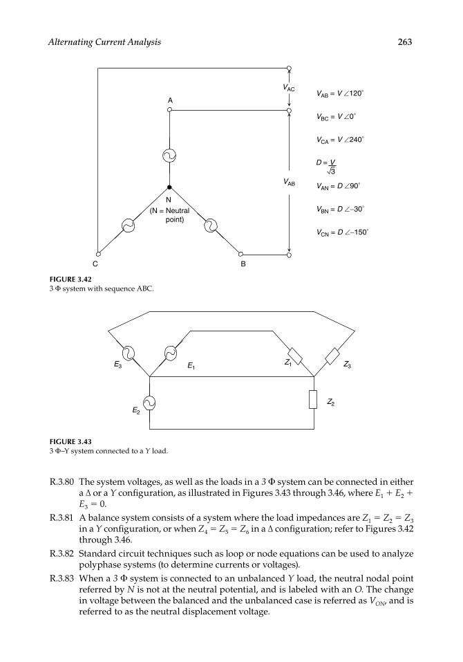
Alternating Current Analysis 263
R.3.80 The system voltages, as well as the loads in a 3 Φ system can be connected in either a ∆ or a Y confi guration, as illustrated in Figures 3.43 through 3.46, where E1 + E2 + E3 = 0.
R.3.81 A balance system consists of a system where the load impedances are Z1 = Z2 = Z3 in a Y confi guration, or when Z4 = Z5 = Z6 in a ∆ confi guration; refer to Figures 3.42 through 3.46.
R.3.82 Standard circuit techniques such as loop or node equations can be used to analyze polyphase systems (to determine currents or voltages).
R.3.83 When a 3 Φ system is connected to an unbalanced Y load, the neutral nodal point referred by N is not at the neutral potential, and is labeled with an O. The change in voltage between the balanced and the unbalanced case is referred as VON, and is referred to as the neutral displacement voltage.
FIGURE 3.423 Φ system with sequence ABC.
C
VAC
B
A
N
(N = Neutralpoint)
VAB
VAB = V ∠120°
VBC = V ∠0°
VAN = D ∠90°
VBN = D ∠−30°
VCN = D ∠−150°
VCA = V ∠240°
D = V3
FIGURE 3.433 Φ–Y system connected to a Y load.
Z2
Z3Z1E1
E3
E2
CRC_47760_CH003.indd 263CRC_47760_CH003.indd 263 7/23/2008 1:27:41 PM7/23/2008 1:27:41 PM

264 Practical MATLAB® Applications for Engineers
R.3.84 The magnitude of the line currents in a balanced 3 Φ system, as well as the voltage drops across the loads are equal, and the phases are evenly spaced by 120°.
R.3.85 The magnitude of the voltages and currents in an unbalanced 3 Φ circuit can vary considerably across the load in which the line currents are not equal and the phases are no longer evenly spaced by 120°.
FIGURE 3.453 Φ–∆ system connected to a ∆ load.
Z6
Z5
E2
E3
E1
Z4
FIGURE 3.463 Φ–∆ system connected to a Y load.
E2
E3
E1
Z2 Z3
Z1
FIGURE 3.443 Φ–Y system connected to a ∆ load.
Z6
Z4Z5E1
E3
E2
CRC_47760_CH003.indd 264CRC_47760_CH003.indd 264 7/23/2008 1:27:42 PM7/23/2008 1:27:42 PM

Alternating Current Analysis 265
R.3.86 The example shown in Figure 3.47 illustrates the general approach employed to solve for all the currents (load and line) in a typical polyphase balanced network. The voltage specs are
V12 = 120 ∠0°
V23 = 120 ∠−120°
V31 = 120 ∠120° (in volts)
The analysis shown in the following is for the load specs for the following structures:a. A ∆ impedance confi guration shown in Figure 3.47 with
Z12 = Z23 = Z31 = j10
b. A Y impedance confi guration shown in Figure 3.48 with
Z1 = Z2 = Z3 = j10
ANALYTICAL Solution
Part a
Applying Ohm’s law to the circuit shown in Figure 3.47, the following currents can be evaluated by
IVZ j12
12
12
120 010
120 010 90
12 90
∠ ∠∠
∠ A
IVZ23
23
23
120 12010 90
12 120 90 12 210
∠∠
∠ ∠( ) A
I23 = 12 ∠150°
IVZ31
31
31
120 12010 90
12 120 90 12 30
∠∠
∠ ∠( ) A
FIGURE 3.473 Φ system connected to a ∆ load with Z12 = Z23 = Z31 = j10.
+
−V23
V31
V12Z12
Z13
Z32
I1
I3
I31
I12
I23
I2 2
3
+
−
−
+
1
•
•
•
CRC_47760_CH003.indd 265CRC_47760_CH003.indd 265 7/23/2008 1:27:42 PM7/23/2008 1:27:42 PM

266 Practical MATLAB® Applications for Engineers
Then, I1 = I12 − I31
I1 12 90 12 30 12 3 120 ∠ ∠ ∠ A
and I2 = I23 − I12
I2 12 150 12 90 12 3 120 ∠ ∠ ∠ A
and I3 = I31 − I23 = 12 ∠30° − 12 ∠150° A
I3 = 12 √ __
3 ∠0° A
Part b
The system for part b is shown in Figure 3.48.Transforming the Y load into a ∆ confi guration, and making use of the symmetry of
the system, the equivalent impedances are evaluated.
ZZ Z Z Z Z Z
Z121 2 2 3 3 1
3
and since Z1 = Z2 = Z3 = j10, then
ZZZ
Z j j1212
11
33 3 10 30 ( ) Ω
ZZ Z Z Z Z Z
Z231 2 2 3 3 1
1
Z23 = 30j Ω
ZZ Z Z Z Z Z
Z311 2 2 3 3 1
2
and
Z31 = 30j Ω
FIGURE 3.483 Φ system connected to a Y load with Z1 = Z2 = Z3 = 10j.
+
−V23
V31
V12Z2
Z3
Z1
I1
I2 2
+
−
−
+
1
•
•
•• N
CRC_47760_CH003.indd 266CRC_47760_CH003.indd 266 7/23/2008 1:27:42 PM7/23/2008 1:27:42 PM

Alternating Current Analysis 267
Then,
I12120 030 90
4 90
∠∠
∠
I23120 120
30 904 150
∠∠
∠
I31120 120
30 904 30
∠∠
∠
Observe that the solution for part b is based in transforming the problem into one that is similar to part a, and the currents just evaluated (part b) are one-third of the currents of part a, because the loads become three times larger.
The line currents using KCL can be evaluated, and are indicated as follows:
I1 = I12 − I31 + 4 √ __
3 ∠−120° A
I2 = 4 √ __
3 ∠120° A
I3 = 4 √ __
3 ∠0° A
The corresponding voltage drops are indicated as follows:
V1N = I1 * Z = 4 √ __
3 ∠−120° * 10 ∠90° V
V1N = 40 √ __
3 ∠−30° V
V2N = 40 √ __
3 ∠−150° V
V3N = 40 √ __
3 ∠90° V
3.4 Examples
Example 3.1
Create the script fi le XL_XC that returns the following plots:
1. mag[XL(ω)] versus ω 2. mag[XC(ω)] versus ω
for L = 2 H and C = 1 µF, over the frequency range 200 ≤ ω ≤ 2000 rad/s.
MATLAB Solution% Script file: XL _ XC L = 2;
CRC_47760_CH003.indd 267CRC_47760_CH003.indd 267 7/23/2008 1:27:43 PM7/23/2008 1:27:43 PM

268 Practical MATLAB® Applications for Engineers
C = 1e-6;w = [200:50:2000];XL = w*L;XC = 1./(w*C);plot(w,XL,’o’,w, XC,’*’)title(‘[XL(w) and XC(w)] vs w’)xlabel(‘frequency in rad/sec’), ylabel(‘Magnitude in Ohms’)legend(‘XL’,’XC’)grid onhold; plot(w,XL,w,XC)
The script fi le XL_XC is executed and the results are shown in Figure 3.49.
Example 3.2
Evaluate the impedance Z and admittance Y = (1/Z) for the circuit shown in Figure 3.50 fi rst by hand, and then by writing the script fi le Z_Y, for an angular frequency of w = 1 rad/s.
FIGURE 3.49Plots of Example 3.1.
200 400 600 800 1000 1200 1400 1600 1800 20000
500
1000
1500
2000
2500
3000
3500
4000
4500
5000[XL(w) and XC(w)] versus w
frequency in rad/sec
Mag
nitu
de in
Ohm
s
XLXC
FIGURE 3.50Network of Example 3.2.
R = 4 ΩC = 1/5 FL = 2 HZ
w = 1 rad/s
CRC_47760_CH003.indd 268CRC_47760_CH003.indd 268 7/23/2008 1:27:43 PM7/23/2008 1:27:43 PM

Alternating Current Analysis 269
ANALYTICAL Solution
XC() = −j5
XL() = j2
X X XX X
X Xj j
j j jC LC L
C L
( ) ( )// ( )( ) ( )
( ) ( )(
5 25 2
103
ΩΩ)
X() = j 10 ___ 3
Z X RX R
X Rjj
j( ) ( )//( )
( ). *.
. . (
3 33 43 33 4
1 639 1 967 Ω)
and
Y(ω) = 1 _____ Z(ω)
Yj
jj( )
..
. . ( )
3 33 4
13 320 25 3 sie
MATLAB Solution% Script file: Z _ YW = 1;C = 1/5;L = 2;R = 4;XC = -j/(W*C);XL = j*W*L;X = XC*XL/(XC+XL);Z = X*R/(X+R);Y = 1/Z; disp(‘ ^^^^^^^^^^^^^^^^^^^^^^^^^^^^^^^^^^^^^^^^^^^^^^^^^^^^^^^^^^^^^^ ’)disp(‘The impedance Z (in Ohms) and admittance (in Siemens) are given
by :’); Z,Y,disp(‘ ^^^^^^^^^^^^^^^^^^^^^^^^^^^^^^^^^^^^^^^^^^^^^^^^^^^^^^^^^^^^^^ ’)
^^^^^^^^^^^^^^^^^^^^^^^^^^^^^^^^^^^^^^^^^^^^^^^^^^^^^^^^^^^^^^^^^^^^^^The impedance Z (in Ohms) and admittance (in Siemens) are given by:
Z = 1.6393 + 1.9672 Y = 0.2500 - 0.3000i
^^^^^^^^^^^^^^^^^^^^^^^^^^^^^^^^^^^^^^^^^^^^^^^^^^^^^^
Example 3.3
Evaluate the impedance Z of the circuit of Figure 3.51 for ω = 10 rad/s by hand, and by creating the script fi le imp_Z.
CRC_47760_CH003.indd 269CRC_47760_CH003.indd 269 7/23/2008 1:27:43 PM7/23/2008 1:27:43 PM

270 Practical MATLAB® Applications for Engineers
ANALYTICAL Solution
Xj C j
jC( )( / )
1 1
10 1 404
· ·Ω
X = 3 − j4 (Ω)
Then, Z = X//R2.
ZXX
* 1010
3 67 36. ∠ Ω
MATLAB Solution% Script file: imp _ ZW = 10;R1 = 3;R2 = 10;C = 1/40;XC = -j/(W*C);X = R1+XC;Z = X*R2/(X+R2);Zmag = abs(Z);Phase = angle(Z);Phase _ deg = Phase*360/(2*pi);disp(‘ ^^^^^^^^^^^^^^^^^^^^^^^^^^^^^^^^^^^^^^^^^^^^^^^^^^^^^^^^^^^^^ ’)disp(‘Magnitude of Z (in Ohms) and phase (in degrees) is given by :’);ZmagPhase _ degdisp(‘ ^^^^^^^^^^^^^^^^^^^^^^^^^^^^^^^^^^^^^^^^^^^^^^^^^^^^^^^^^^^^^ ’)
The script fi le imp_Z is executed and the results are shown as follows.
FIGURE 3.51Network of Example 3.3.
Z R2 = 10 Ω
R1 = 3 Ω
C = 1/40 F
w = 10 rad/s
CRC_47760_CH003.indd 270CRC_47760_CH003.indd 270 7/23/2008 1:27:44 PM7/23/2008 1:27:44 PM

Alternating Current Analysis 271
>> imp _ Z
^^^^^^^^^^^^^^^^^^^^^^^^^^^^^^^^^^^^^^^^^^^^^^^^^^^^^^^^^^^^^^^^^^^^^
Magnitude of Z (in Ohms) and phase (in degrees) is given by : Zmag = 3.6761 Phase _ deg = -36.0274
^^^^^^^^^^^^^^^^^^^^^^^^^^^^^^^^^^^^^^^^^^^^^^^^^^^^^^^^^^^^^^^^^^^^^
Example 3.4
Evaluate by hand and by using MATLAB the voltage v(t) across the series RL circuit shown in Figure 3.52, if the current is i(t) = 5 cos(100t) A.
ANALYTICAL Solution
I = 5 ∠0°
Z = 40 + j * 100 * 0.3 = 40 + j30
V = Z * I = (40 + j30) * 5 ∠0° = 250 ∠(36.52°)
then
v(t) = 250 cos(100t + 36.87°)
MATLAB Solution% Script file: vol _ RLW=100;Z=40+j*W*.3;V=5*Z;Vmax=abs(V);Phase=angle(V);Phasedegree=Phase*180/pi;% Print resultsdisp(‘ ^^^^^^^^^^^^^^^^^^^^^^^^^^^^^^^^^^^^^^^^^^^^^^^^^^^^^^^^^^ ’)disp(‘The peak value (in volts) and the phase (in degrees) of v(t)
are=’);Vmax,Phasedegree,disp(‘ ^^^^^^^^^^^^^^^^^^^^^^^^^^^^^^^^^^^^^^^^^^^^^^^^^^^^^^^ ’)
FIGURE 3.52Network of Example 3.4.
R1 = 40 Ω
L = 0.3 H
v (t )
i(t )
CRC_47760_CH003.indd 271CRC_47760_CH003.indd 271 7/23/2008 1:27:44 PM7/23/2008 1:27:44 PM

272 Practical MATLAB® Applications for Engineers
The script fi le vol_RL is executed and the results are as follows:
>> vol _ RL
^^^^^^^^^^^^^^^^^^^^^^^^^^^^^^^^^^^^^^^^^^^^^^^^^^^^^^^^^^^^^^^The peak value (in volts) and the phase (in degrees) of v(t) are=
Vmax = 250
Phasedegree = 36.8699
^^^^^^^^^^^^^^^^^^^^^^^^^^^^^^^^^^^^^^^^^^^^^^^^^^^^^^^^^^^^^^^
The preceding result means that v(t) = 250 cos(100t + 36.8699°) V.
Example 3.5
Evaluate the current i(t) for the circuit shown in Figure 3.53 by hand, and by using MATLAB.
ANALYTICAL Solution
V = 200 ∠0°, Z = 20 – j _____________
125 ∗ 10–6 ∗ 500 = 20 – j16
then
IVZ j j
200
20 1650
5 47 8 38 6. .∠ A
Therefore, i(t) = 7.8 cos(500t + 38.6°) A.
MATLAB Solution>> W = 500;>> V = 200;>> R = 20;>> C = 125e-6
FIGURE 3.53Network of Example 3.5.
C = 125 µ F
i (t )
v (t ) = 200 cos(500 t ) V R = 20 Ω
CRC_47760_CH003.indd 272CRC_47760_CH003.indd 272 7/23/2008 1:27:44 PM7/23/2008 1:27:44 PM

Alternating Current Analysis 273
C = 1.2500e-004
>> XC = -j/(W*C)
XC = 0 -16.0000I
>> Z = R+XC
Z = 20.0000 -16.0000I
>> Zmag = abs(Z);>> phase = -angle(Z)*180/pi
phase = 38.6598
>> I = V/Zmag;>> % Print results>> disp(‘The peak value of the current (in amps) is =’), disp(I);>> disp(‘with a phase angle(in degrees) of =’), disp(phase)
The peak value of the current (in amps) is = 7.8087 with a phase angle (in degrees) of = 38.6598
The meaning of the aforementioned results is that the current is given by
i(t) = 7.8087 cos(500t + 38.6598°) A
Example 3.6
Create the script fi le curr_volt that returns the plots of v(t) versus t and i(t) versus t, over the range 0 ≤ t ≤ 0.06 s, for the circuit shown in Figure 3.54, where i(t) = 5 sin(300t) A.
FIGURE 3.54Network of Example 3.6.
L = 60 mH
i (t )
v (t )
R = 10 Ω
CRC_47760_CH003.indd 273CRC_47760_CH003.indd 273 7/23/2008 1:27:44 PM7/23/2008 1:27:44 PM
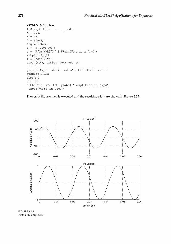
274 Practical MATLAB® Applications for Engineers
MATLAB Solution% Script file: curr _ voltW = 300;R = 19;L = 60e-3;Ang = W*L/R;t = [0:.0001:.06];V = (R^2+(W*L) 2) .5*5*sin(W.*t+atan(Ang)); subplot(2,1,1)I = 5*sin(W.*t);plot (t,V), title(‘ v(t) vs. t’)grid onylabel(‘Amplitude in volts’), title(‘v(t) vs.t’)subplot(2,1,2)plot(t,I)grid ontitle(‘i(t) vs. t’), ylabel(‘ Amplitude in amps’)xlabel(‘time in sec.’)
The script fi le curr_volt is executed and the resulting plots are shown in Figure 3.55.
FIGURE 3.55Plots of Example 3.6.
200
100
0
0
0
0.01 0.02 0.03 0.04 0.05 0.06
0 0.01 0.02 0.03
time in sec.
0.04 0.05 0.06
−100
−200
−5
v(t) versus t
i(t) versus t
Am
plitu
de in
vol
tsA
mpl
itude
in a
mps
5
CRC_47760_CH003.indd 274CRC_47760_CH003.indd 274 7/23/2008 1:27:45 PM7/23/2008 1:27:45 PM

Alternating Current Analysis 275
Example 3.7
Let the current in the RC circuit shown in Figure 3.56 be i(t) = 5 sin(200t) A. Create the script fi le curr_vol_RC that returns the plots of v(t) versus t and i(t) versus t, over the range 0 ≤ t ≤ 0 .1 s.
MATLAB Solution% Script file: curr _ vol _ RC clfW = 200;R = 0.5e5;C = 10e-8;Ang = 1/(W*C*R);t = 0:.001:.1;V = (R^2+(1/W*C) 2) .5*5*sin(W.*t-atan(Ang));I =5*sin(W.*t);subplot(2,1,1)plot(t,V)ylabel(‘Ampitude[v(t)]’);xlabel(‘time in seconds’);title(‘v(t) vs. t ’)subplot(2,1,2)plot(t,I)title(‘i(t) vs. t ’)xlabel(‘time in seconds’);ylabel(‘Amplitude[i(t)]’)
The script fi le curr_vol_RC is executed and the returning plots are shown in Figure 3.57.
C = 10*10−8 F
R = 0.5*105 Ω
i (t ) = 5 sin(200 t ) A
v (t )
FIGURE 3.56Network of Example 3.7.
CRC_47760_CH003.indd 275CRC_47760_CH003.indd 275 7/23/2008 1:27:45 PM7/23/2008 1:27:45 PM

276 Practical MATLAB® Applications for Engineers
Example 3.8
Given the following periodic functions defi ned over one period (T):
a. f1(t) = 5 cos((2π/3)t), with T = 3 s b. f2(t) = t, for 0 ≤ t ≤ 1, with T = 1 s
c. f tt
t T3
1 0 0 50 0 5 1 1
( ).
. s
with
Create the script fi le ave_rms_sym that returns the following plots over the range −1 ≤ t ≤ 3:
a. f1(t) versus t b. f2(t) versus t c. f3(t) versus t
Also evaluate the average and the RMS (effective) value for each one of the preceding functions using
a. a symbolic approach by creating the script fi le ave_rms_sym (use int) b. a numerical solution by creating the script fi le ave_rms_num (use trapz)
Recall that the average value of the arbitrary f(t) is given by
FT
f t dtAVE
T
1
0
( )∫
and its RMS value is given by
FT
f t dtRMS
T
1 2
0
( )∫
FIGURE 3.57Plots of Example 3.7.
0
0 0.01 0.02 0.03 0.04 0.05 0.06 0.07 0.08 0.09 0.1
0 0.01 0.02 0.03 0.04 0.05 0.06 0.07 0.08 0.09 0.1
−5
−4
−2
0
2
4v(t) versus t
i(t) versus t
Am
plitu
de [i
(t)]
Am
plitu
de [v
(t)]
5
× 105
time in seconds
time in seconds
CRC_47760_CH003.indd 276CRC_47760_CH003.indd 276 7/23/2008 1:27:46 PM7/23/2008 1:27:46 PM

Alternating Current Analysis 277
MATLAB Solution% Script file : ave _ rms _ sym% returns the functions f1,f2,& f3% and computes the average and rms values of f1,f2 & f3% using symbolic (int) techniquex = linspace(-3,3,100);f1t = 5.*cos(2*pi./3.*x);subplot(3,1,1)plot(x,f1t);title(‘Plots of f1(t),f2(t) & f3(t)’);ylabel(‘f1(t)’),axis([-3 3 -6 6]);subplot(3,1,2)a = linspace(0,1,25);y = [a a a a];x=linspace(-1,3,100);plot(x,y);ylabel(‘f2(t)’);axis([-1 3 -.5 1.5]);b = [ones(1,12) zeros(1,13)];bb = [b b b b];subplot(3,1,3)plot(x,bb);ylabel(‘f3(t)’);axis([-1 3 -.5 1.5]); xlabel(‘time’); % Figure 3.58syms t;w = 2*pi/3;T = 2*pi/w;f1ave=1/T*int(5*cos(w*t),0,T); % part(a)disp(‘****************************************************’);disp(‘************Symbolic Results (using int )*********’);disp(‘****************************************************’);disp(‘The average value of f1(t) is =’);ans1=vpa(f1ave);disp(ans1);f1rms=sqrt(1/T*int(25*cos(w*t) 2,0,T)); % part(b)disp(‘The RMS value of f1(t) is =’);ans2=vpa(f1rms);disp(ans2);T1=1;w1=2*pi/T1;Vave2 = 1/T1*int(t,0,T1);%part(b)disp(‘The average value of f2(t) is =’);ans3 = vpa(Vave2); disp(ans3);Vrms2 =sqrt(1/T1*int(t^2,0,T1));disp(‘The RMS value of f2(t) is =’);ans4 = vpa(Vrms2); disp(ans4);w2 = 2*pi/T1;Vave3 =1/T1*int(sym(‘Heaviside(t)’),0,T1/2); %part(c)disp(‘The average value of f3(t) is =’);ans5 = vpa(Vave3);disp(ans5);Vrms3 =sqrt(1/T1*int(sym(‘Heaviside(t) 2’),0,T1/2));disp(‘The RMS value of f3(t) is =’);ans6 = vpa(Vrms3);disp(ans6);disp(‘****************************************************’);
The results of executing the script fi le ave_rms_sym are shown as follows:>> ave_rms_sym
************************************************************************* Symbolic Results ( using int) **************************************************************************
The average value of f1(t) is = 0
CRC_47760_CH003.indd 277CRC_47760_CH003.indd 277 7/23/2008 1:27:46 PM7/23/2008 1:27:46 PM

278 Practical MATLAB® Applications for Engineers
The RMS value of f1(t) is = 3.5355339059327376220042218105243The average value of f2(t) is = .50000000000000000000000000000000The RMS value of f2(t) is = .57735026918962576450914878050196The average value of f3(t) is = .50000000000000000000000000000000The RMS value of f3(t) is = .70710678118654752440084436210485
**********************************************************************
% Script file: ave _ rmst _ num% evaluates the average and rms values of f1,f2 and f3% using numerical techniques (trapz)t1= linspace(0,3,100);y1= 5*cos(2*pi/3*t1);avecos =1/3*trapz(t1,y1);y1sq = y1. 2;rmscos = sqrt(1/3*trapz(t1,y1sq));t2 =linspace(0,1,100);y2 = t2;avesaw = trapz(t2,y2);y2sq = y2. 2;rmssaw = sqrt(trapz(t2,y2sq));y3 = [ones(1,50) zeros(1,50)];avesqr = trapz(t2,y3);y3sq = y3. 2;rmssqr = sqrt(trapz(t2,y3sq));disp(‘*********************************************************’);disp(‘ ********* Numerical Results (using trapz)***********’);disp(‘*********************************************************’);disp(‘ ’)disp(‘The average value of f1(t) is =’)disp(avecos)disp(‘The rms value of f1(t) is =’)disp(rmscos)disp(‘ ’)disp(‘The average value of f2(t) is =’)disp(avesaw)disp(‘The rms value of f2(t) is =’)disp(rmssaw)disp(‘ ’)disp(‘The average value of f3(t) is =’)disp(avesqr)disp(‘The rms value of f1(t) is =’)disp(rmssqr)disp(‘**************************************************’)
The script fi le ave_rms_num is executed and the results are as follows:
>> ave _ rms _ num
***************************************************************** Numerical Results (using trapz) **********************************************************************
CRC_47760_CH003.indd 278CRC_47760_CH003.indd 278 7/23/2008 1:27:46 PM7/23/2008 1:27:46 PM

Alternating Current Analysis 279
The average value of f1(t) is = -6.8464e-016The rms value of f1(t) is = 3.5355The average value of f2(t) is = 0.5000The rms value of f2(t) is = 0.5774The average value of f3(t) is = 0.5000 The rms value of f1(t) is = 0.7071
*********************************************************
Observe that the numerical results fully agree with the symbolic results.
Example 3.9
Create the script fi les circ_Fig_359 and circ_Fig_360 that return for the circuits shown in Figures 3.59 and 3.60, the following plots:
1. |Z(ω)| versus ω 2. ∠Z(ω) versus ω
−3 −2 −1 0 1 2 3−5
0
5
Plots of f1(t), f2(t), & f3(t)
f1 (
t)
−1 −0.5 0 0.5 1 1.5 2 2.5 3−0.5
0
0. 5
1
1.5
f2 (
t)
−1 −0.5 0 0.5 1 1.5 2 2.5 3−0.5
0
0.5
1
1.5
f3 (
t)
time
(a)
(b)
(c)
FIGURE 3.58 Plots of the periodic functions of Example 3.8 (a, b, c).
CRC_47760_CH003.indd 279CRC_47760_CH003.indd 279 7/23/2008 1:27:46 PM7/23/2008 1:27:46 PM

280 Practical MATLAB® Applications for Engineers
ANALYTICAL Solution
For the circuit shown in Figure 3.59 (part a),
ZC j
j RC j LC( )
( / )( )( ) ( / )( ) ( / )
11 12
For R = L = C = 1,
Zj
j j( )
( )( ) ( )
2 1
For the circuit shown in Figure 3.60 (part b),
ZR j C j R LC
j LC( )
( ) ( / )( ) ( / )( ) ( / )
2
2
11
For R = 1000 Ω, L = 30 mH, and C = 0.47 µF (Figure 3.61),
Zj j
j( )
( ).
( ).
( )
10001
0 47 101000
30 10 0 47 102
6 3 6
2
**
** * *
130 10 0 47 103 6* * *.
MATLAB Solution% Script file: circ _ Fig _ 359% R, L, and C in parallel% R = C = L = 1.echo on;w = 0:0.1:5;num = [0 0 1];den = [1 1 1];ZW = freqs (num, den, w);subplot(2, 1, 1);plot(w, abs(ZW));grid on;title(‘Magnitude and phase of Z(w)’);xlabel(‘w(rad/sec)’);ylabel(‘magnitude’);subplot(2, 1, 2);plot(w, angle(ZW)*180/pi); % Figure 3.61xlabel(‘w(rad/sec)’);ylabel(‘phase in degrees’);grid on;
C RL
Z
FIGURE 3.59Network with R = C = L = 1, over the range 0 ≤ ω ≤ 5 rad/s of Example 3.9.
C
R
LZ
FIGURE 3.60Network with R = 1000 Ω, L = 30 mH, and C = 0.47 µF, over the range 7500 ≤ ω ≤ 9500 rad/s of Example 3.9.
CRC_47760_CH003.indd 280CRC_47760_CH003.indd 280 7/23/2008 1:27:47 PM7/23/2008 1:27:47 PM

Alternating Current Analysis 281
0 0.5 1 1.5 2 2.5 3 3.5 4 4.5 50
0.5
1
1.5Magnitude and phase of Z(w)
w (rad/sec)
0 0.5 1 1.5 2 2.5 3 3.5 4 4.5 5w (rad/sec)
mag
nitu
de
−200
−150
−100
−50
0
phas
e in
deg
rees
FIGURE 3.61Plots for the circuit of Figure 3.59.
% Script file: circ _ Fig _ 360echo on;w = 7500:50:9500;R = 1000;L = 30e-3;C = 0.47e-6;num = [R 1/C R/(L*C)];den = [1 0 1/(L*C)];ZW = freqs(num, den, w);subplot(2, 1, 1);plot(w, abs(ZW));grid on;title(‘Magnitude and phase of Z(w)’);xlabel(‘w(rad/sec)’);ylabel(‘magnitude’);subplot(2, 1, 2);plot(w, angle(ZW)*180/pi);xlabel(‘w(rad/sec)’);ylabel(‘phase in degrees’);grid on; % Figure 3.62
CRC_47760_CH003.indd 281CRC_47760_CH003.indd 281 7/23/2008 1:27:47 PM7/23/2008 1:27:47 PM

282 Practical MATLAB® Applications for Engineers
Example 3.10
Given the current and voltage shown in the circuit diagram of Figure 3.63, write a pro-gram that returns the following:
1. Plots of i(t) versus t, v(t) versus t, and p(t) versus t over 0 ≤ t ≤ 0.01 2. Evaluate using MATLAB
a. The average power delivered to the load b. The RMS value of i(t) and v(t) by using numerical techniques and verify the
results by VRMS = Vm ∗ 0.707 and IRMS = Im ∗ 0.707 c. The PF
0
1
2
3
4
5× 10⁴ Magnitude and phase of Z(w)
mag
nitu
de
7500 8000 8500 9000 9500−100
−50
0
50
100
w (rad/sec)
7500 8000 8500 9000 9500w (rad/sec)
phas
e in
deg
rees
FIGURE 3.62Plots for the circuit of Figure 3.60.
υ(t ) = 9 cos(200*π*t + 45°)V
i (t ) = 5 sin(200*π*t + 60°)
Z
A
FIGURE 3.63Network of Example 3.10.
CRC_47760_CH003.indd 282CRC_47760_CH003.indd 282 7/23/2008 1:27:47 PM7/23/2008 1:27:47 PM

Alternating Current Analysis 283
MATLAB Solution>> % Instantaneous power plot>> T= 2*pi/(200*pi);>> X= [0:.01:1];>> t = X.*T;>> IT = 5*cos(200*pi*t+pi/3);>> VT = 9*cos(200*pi*t+pi/4);>> PT = IT.*VT;>> plot(t,PT,’o’,t,VT,’*’,t,IT,’+’); % Figure 3.64>> legend(‘i(t)’, ‘v(t)’, ‘p(t)’)>> grid on>> title(‘Instantaneous Power, Current, and Voltage’)>> xlabel(‘time in seconds’),ylabel(‘ Amplitudes of P, I, &V’)>> VTSQ=VT. 2; % v(t) 2>> IntVTSQ = .01*T*(trapz(VTSQ)) % integral ofv(t) 2
IntVTSQ = 0.4050
>> ITSQ = (5*cos(200*pi*t+pi/3)). 2; % i(t) 2>> IntITSQ = .01*T*(trapz(ITSQ)) % integral of i(t) 2
IntITSQ = 0.1250
>> VRMS = sqrt((IntVTSQ)/T) % RMS value of voltage
VRMS = 6.3640
>> IRMS = sqrt((IntITSQ)/T) % RMS value of current.
IRMS = 3.5355
>> % average power using trapz>> PowerWave = .01*T*trapz(PT)/T
PowerWave = 21.7333
>> % Power Factor numerical >> PF = PowerWave/(VRMS*IRMS)
PF = 0.9659
>> % verify results analytically >> VRMSANA = 9*.707
VRMSANA = 6.3630
>> IRMSANA = 5*.707
IRMSANA = 3.5350
CRC_47760_CH003.indd 283CRC_47760_CH003.indd 283 7/23/2008 1:27:48 PM7/23/2008 1:27:48 PM

284 Practical MATLAB® Applications for Engineers
>> PowerWaveAna = (45/2)*cos(15*pi/180)
PowerWaveANA = 21.7333
>> % results are printed for comparisons
>> fprintf(‘Average Power, Numerical:%f\n’,PowerWave)
Average Power, Numerical: 21.733331
>> fprintf(‘Average Power, Analytical:%f\n’,PowerWaveANA)
Average Power, Analitical: 21.7333
>> fprintf(‘VRMS, Numerical:%f\n’,VRMS)
VRMS, Numerical: 6.3640
>> fprintf(‘VRMS, Analytical:%f\n’,VRMSANA)
VRMS, Analytical: 6.3630
>> fprintf(‘IRMS, Numerical:%f\n’,IRMS)
IRMS, Numerical: 3.5355
>> fprintf (‘IRMS, Analytical:%f\n’,IRMANA)
IRMS, Analytical: 3.5350
>> fprintf (‘PowerFactor, PF:%f\n’,PF)
PowerFactor,PF: 0.965926
Observe that the analytical results fully agree with the numerical results.
0 0.001 0.002 0.003 0.004 0.005 0.006 0.007 0.008 0.009 0.01−10
0
10
20
30
40
50
time in seconds
Am
plitu
des
of P
, I, &
V
Instantaneous Power, Current, and Voltage
i(t)v(t)p(t)
FIGURE 3.64Plots of i(t), v(t), and p(t) of Example 3.10.
CRC_47760_CH003.indd 284CRC_47760_CH003.indd 284 7/23/2008 1:27:48 PM7/23/2008 1:27:48 PM

Alternating Current Analysis 285
Example 3.11
Write a MATLAB program that returns
1. The phasor diagram of the voltages V(Applied), VL, VC, and VR of the circuit shown in Figure 3.65
2. The angle between the I and V 3. Verify KVL, that is, V = VL + VC + VR
R = 100 Ω
I
C = 40 µF
L = 0.5 HV = 220, f = 60 Hz
FIGURE 3.65Network of Example 3.11.
MATLAB Solution>> V = 220;>> R = 100;>> C = 40e-6;>> L = .5;>> Omega = 2*pi*60;>> Z = R+j*((L*Omega)-1/(C*Omega));>> Magnitude = abs(Z);>> Phase = 180*angle(Z)/pi;>> I = V/Z;>> I = abs(I);>> VR = I*R;>> VL = j*L*Omega*I;>> VC = -j*I/(C*Omega);>> Vapplied = VR+VL+VC; % the result should be 220 (KVL)>> Check _ KVL = abs(VApplied)
Check _ KVL = 220.0000
>> phase _ in _ deg = 180*angle(VApplied)/pi
phase _ in _ deg = 50.7011
>> % construction of the phasor diagram>> L(1) = 0;>> L(2) = VR;>> L(3) = VR+VL;>> L(4) = VR+VC;>> Voltage = [0 VApplied];>> axis(‘square’)>> plot(real(L), imag(L), real(Voltage), imag(Voltage))>> grid on>> xlabel(‘Real Axis’), ylabel(‘Imaginary Axis’)>> title(‘Phasor Diagram’) (Figure 3.66)
CRC_47760_CH003.indd 285CRC_47760_CH003.indd 285 7/23/2008 1:27:48 PM7/23/2008 1:27:48 PM

286 Practical MATLAB® Applications for Engineers
Example 3.12
Create the script fi le phasor_time_plots that returns the circuit diagram shown in Fig-ure 3.67, the following plots:
1. The phasor diagram for VS, VC, and VR
2. vS(t) versus t, vR(t) versus t, and vC(t) versus t
0−100
−50
20 40 60 80 100 120 140Real Axis
0
50
100
150
200
250
300
Imag
inar
y A
xis
Phasor Diagram
FIGURE 3.66Phasor diagram of Example 3.11.
R = 1 Ω
C = 1 µFvs(t ) = sin(1000*t ) V
FIGURE 3.67Network of Example 3.12.
MATLAB Solution% Script file: phasor _ time _ plotsclfVS = 1;R = 1e3;C = 1e-6;
CRC_47760_CH003.indd 286CRC_47760_CH003.indd 286 7/23/2008 1:27:49 PM7/23/2008 1:27:49 PM

Alternating Current Analysis 287
F = 1000;W = 2*pi*F;ZC = -j/(W*C);ZT = R+ZC;I = VS/ZT;VR = R*I;VC = ZC*I;subplot(2,1,1)% Phasors diagram.VSS = [0 VS];VVC = [0 VC];VVR = [0 VR];plot(real(VSS),imag(VSS),’*’,real(VVC),imag(VVC),’+’,real(VVR),imag(VVR),’o’);xlabel(‘Real’), ylabel(‘Imaginary’),title(‘Phasor Diagram (Example 3.12)’); % Figure 3.68 (top)grid onhold ; %hold plot plot(real(VSS), imag(VSS), real(VVC),imag(VVC),real(VVR),imag(VVR));legend(‘VS’, ‘VC’, ‘VR’);% Check the Phasor Diagram by applying Kirchhoffs Voltage Law.disp(‘**********************************************************’)disp(‘****Check the Phasor Diagram results by applying *****’)disp(‘*********** Kirchhoffs Voltage Law *******************’)Check _ Voltage = VR+VCdisp(‘**********************************************************’)disp(‘ (Note:Check _ V should be equal to VS=1.)’)T = 1/F;t = [0:2*T/50:2*T]; % t for 2 periodsVS = sin(W.*t);VRT = abs(VR)*sin(W.*t+angle(VR));VCT = abs(VC)*sin(W.*t+angle(VC));subplot (2,1,2)plot (t,VS,’o’,t,VRT,’*’,t,VCT,’+’)xlabel (‘time in seconds’),ylabel (‘Amplitude in Volts’)title(‘Voltages of the RC Circuit of Example 3.12’); % Figure 3.68 (bottom)grid onlegend(‘vs(t)’,’vr(t)’,’vc(t)’)
The MATLAB script fi le phasor_time_plots is executed, and the results are shown as follows:
>> phasor _ time _ plots
Current plot held*************************************************************Check the Phasor Diagram results by applying******************* Kirchhoffs Voltage Law ******************
Check _ Voltage = 1
*****************************************************
(note that the correct result is verified by Check _ Voltage=1)
CRC_47760_CH003.indd 287CRC_47760_CH003.indd 287 7/23/2008 1:27:49 PM7/23/2008 1:27:49 PM

288 Practical MATLAB® Applications for Engineers
Example 3.13
Create the script fi le impedance_ plots that returns for the series RLC circuit shown in Figure 3.69, over the range 100 ≤ ω ≤ 10,000 rad/s, the following plots:
1. |Z(ω)| versus ω 2. ∠Z(ω) versus ω 3. Repeat parts 1 and 2 for the case where the three elements (R, L, and C) are connected
in parallel
R = 10 Ω
C = 12.5 µF
L = 5 mH100 rad/s ≤ w ≤ 10,000 rad/s
FIGURE 3.69Network of Example 3.13.
0.2
0.1
0
0 0.1
1
0
0.2 0.3 0.4 0.5
0.5
−0.5
−1
Real
Voltage of the RC Circuit of Example 3.12
0.6 0.7 0.8 0.9 1
0 0.2 0.4 0.6 0.8 1
time in seconds
1.2 1.4 1.5 1.8
× 10−3
2
−0.1
−0.2
Am
plitu
de in
Vol
tsIm
agin
ary
VS
VC
VR
vs(t)
vr(t)
vc(t)
Phasor Diagram (Example 3.12)
FIGURE 3.68Plots of Example 3.12.
CRC_47760_CH003.indd 288CRC_47760_CH003.indd 288 7/23/2008 1:27:49 PM7/23/2008 1:27:49 PM
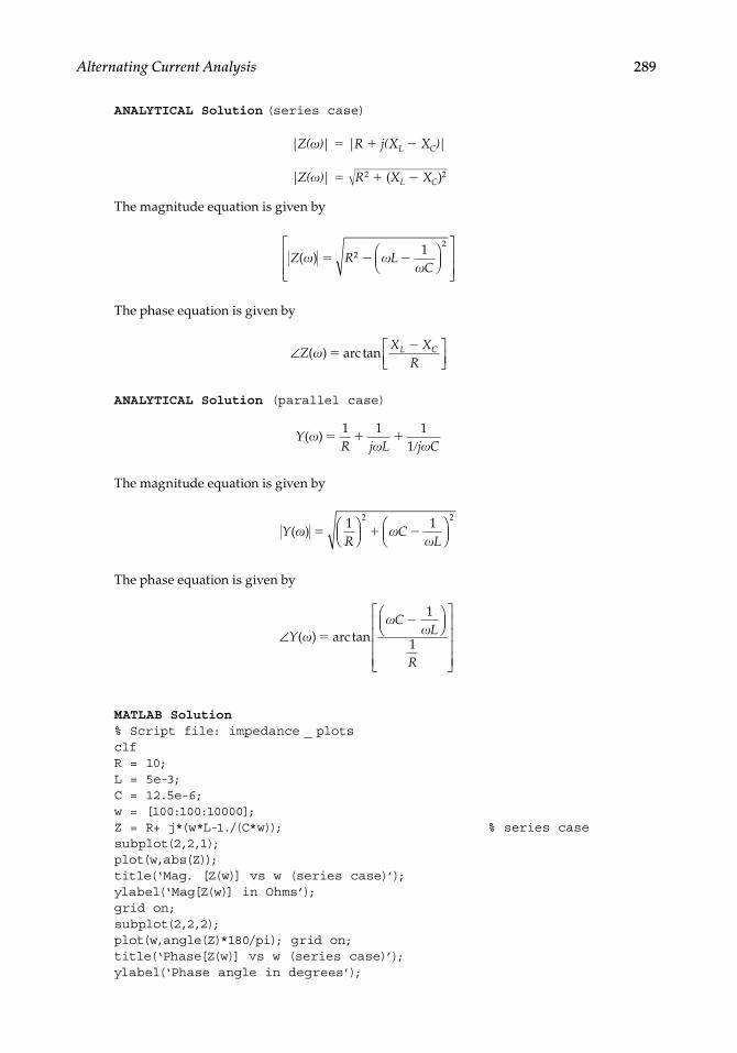
Alternating Current Analysis 289
ANALYTICAL Solution (series case)
|Z()| = |R + j(XL − XC)|
|Z()| = √ _______________
R2 + (XL − XC)2
The magnitude equation is given by
Z R LC
( )
221
The phase equation is given by
∠
ZX X
RL C( ) arc tan
ANALYTICAL Solution (parallel case)
YR j L j C
( )
1 1 11
The magnitude equation is given by
YR
CL
( )
1 1 2
2
The phase equation is given by
∠
YC
L
R
( ) arc tan
1
1
MATLAB Solution% Script file: impedance _ plots clfR = 10;L = 5e-3;C = 12.5e-6;w = [100:100:10000];Z = R+ j*(w*L-1./(C*w)); % series casesubplot(2,2,1);plot(w,abs(Z));title(‘Mag. [Z(w)] vs w (series case)’);ylabel(‘Mag[Z(w)] in Ohms’);grid on;subplot(2,2,2);plot(w,angle(Z)*180/pi); grid on;title(‘Phase[Z(w)] vs w (series case)’);ylabel(‘Phase angle in degrees’);
CRC_47760_CH003.indd 289CRC_47760_CH003.indd 289 7/23/2008 1:27:49 PM7/23/2008 1:27:49 PM

290 Practical MATLAB® Applications for Engineers
XC = -j./(w*C);XL = j*w*L;ZLC = XC.*XL./(XC+XL);ZRLC = R.*ZLC./(R+ZLC); % parallel casesubplot (2,2,3);plot (w,abs(ZRLC));title(‘Mag. [Z(w)] vs w (parallel case)’);xlabel (‘w in rad/sec’);ylabel (‘Mag[Z(w)] in Ohms’);grid on;subplot(2,2,4);plot(w,angle(ZRLC)*180/pi); grid on;title(‘Phase[Z(w)] vs w (parallel case)’);xlabel(‘w in rad/sec’); ylabel(‘Phase angle in degrees’);
The script fi le impedance_plots is executed, and the results are indicated in Figure 3.70.
0 5000 10,0000
200
400
600
800Mag. [Z(w)] versus w (series case)
Mag
[Z(w
)] in
Ohm
s
0 5000 10,000−100
−50
0
50
100Phase[Z(w)] versus w (series case)
Pha
se a
ngle
in
degr
ees
0 5000 10,0000
2
4
6
8
10Mag. [Z(w)] versus w (parallel case)
Mag
[Z(w
)] in
Ohm
s
0 5000 10,000−50
0
50
100Phase[Z(w)] versus w (parallel case)
w in rad/secw in rad/sec
Pha
se a
ngle
in
degr
ees
FIGURE 3.70Plots of Example 3.13.
Example 3.14
Analyze the circuit diagram shown in Figure 3.71, and obtain by hand the system loop equations, as well as the matrix loop equation.
Create the script fi le loops that returns
1. The system matrices Z and V 2. The loop currents I1, I2, and I3, in phasor form 3. The instantaneous loop currents i1(t), i2(t), and i3(t)
CRC_47760_CH003.indd 290CRC_47760_CH003.indd 290 7/23/2008 1:27:49 PM7/23/2008 1:27:49 PM

Alternating Current Analysis 291
ANALYTICAL Solution
The circuit of Figure 3.71 is transformed into the phasor circuit diagram shown in Figure 3.72.
The three loop equations are
( ) * *10 201
2020 0 50 01 2 3 j I I I
∠
20 20 30140
140
01 2 3I j I j I
* *
0140
10140
9 451 2 3I j I j I
∠* *
The matrix loop equation is given by
( ) ( / )( ( / )) ( / )
( / )
10 20 1 20 20 020 20 30 1 40 1 400 1 40 10
j
j j
j j(( / )*
1 40
5 00
9 45
1
2
3
∠
∠
I
I
I
C2 = 4 Fv1(t ) = 5 cos (10*t) V
v2(t ) = 9 cos(10*t + 45°) V
I1 I2 I3
R1 = 10 Ω R3 = 10 Ω
R2 = 20 Ω
L1 = 3 HC1 = 2 F
FIGURE 3.71Network of Example 3.14.
5 90° V 45° V
XL = j 30 ΩXc1 = −j (1/20) Ω
Xc2 = −j (1/40) Ω
I1 I2 I3
R1 = 10 Ω
R2 = 20 Ω
R3 = 10 Ω
FIGURE 3.72Phasor circuit diagram of Example 3.14.
CRC_47760_CH003.indd 291CRC_47760_CH003.indd 291 7/23/2008 1:27:50 PM7/23/2008 1:27:50 PM

292 Practical MATLAB® Applications for Engineers
Note that the aforementioned matrix equations can be expressed as [Z] * [I] = [V], where
Z
j
j j
j
( ) ( / )( ( / )) ( / )
( / )
10 20 1 20 20 020 20 30 1 40 1 400 1 40 10 j( / )1 40
and
V
5 00
9 45
∠
∠
The currents I1, I2, and I3 can be evaluated by using the following MATLAB matrix relation
I = inv (Z) * [V]
MATLAB Solution% Script file: loopsdisp(‘**********************************’)disp(‘ System Matrices ’)disp(‘**********************************’)disp(‘The impedance matrix is given by:’)Z = [30-j*1/20 -20 0;-20 20+j*(30-1/40) j*(1/40); 0 j*(1/40) 10-j*(1/40)]A = 9*exp(j*45*pi/180);disp(‘The voltage matrix is given by:’)V= [5; 0; A]disp(‘**********************************’)disp(‘ Loop Currents ’)disp(‘**********************************’)% Solve for loop currents I1, I2 and I3I = inv(Z)*V;% Solve for Magnitude and Phase Angle.I1mag = abs(I(1));I2mag = abs(I(2));I3mag = abs(I(3));I1ang = angle(I(1))*180/pi;I2ang = angle(I(2))*180/pi;I3ang = angle(I(3))*180/pi;% Print currentsdisp(‘ ^^^^^^^^^^^^^^^^^^^^^^^^^^^^^^^^^^^^^^^^^^^^^^^ ’)disp(‘ phasor domain ’)disp(‘ ^^^^^^^^^^^^^^^^^^^^^^^^^^^^^^^^^^^^^^ ’)fprintf(‘The magnitude of the Current I1 (in amps) is :%f\n and its
phase angle in degrees is :%f\n’,I1mag,I1ang)fprintf(‘The magnitude of the current I2 (in amps) is :%f\n and its
phase angle in degrees :%f\n’,I2mag,I2ang)fprintf(‘The magnitude of the current I3 (in amps)is :%f\n and its
phase angle in degrees is :%f\n’,I3mag,I3ang)disp(‘ ^^^^^^^^^^^^^^^^^^^^^^^^^^^^^^^^^^^^^^^^^^^^^^^ ’)disp(‘ time domain ’)disp(‘ ^^^^^^^^^^^^^^^^^^^^^^^^^^^^^^^^^^^^^^^^^^^^^^^ ’)
CRC_47760_CH003.indd 292CRC_47760_CH003.indd 292 7/23/2008 1:27:50 PM7/23/2008 1:27:50 PM

Alternating Current Analysis 293
fprintf(‘The current i1(t)=%fcos(10t %f)amps\n’,I1mag,I1ang)fprintf(‘The current i2(t)=%fcos(10t %f)amps\n’,I2mag,I2ang)fprintf(‘The current i3(t)=%fcos(10t+ %f)amps\n’,I3mag,I3ang)disp(‘*******************************************************’)
The script fi le loops is executed and the results are indicated as follows:
>> loops
***************************************** System Matrices ***************************************** The impedance matrix is given by: Z = 30.0000 - 0.0500i -20.0000 0 -20.0000 20.0000 + 29.9750i 0 + 0.0250i 0 0 + 0.0250i 10.0000 - 0.0250i The voltage matrix is given by: V = 5.0000 0 6.3640 + 6.3640i ******************************************************** Loop Currents ******************************************************** ^^^^^^^^^^^^^^^^^^^^^^^^^^^^^^^^^^^^^^^^^^^^^^^^^^^^^^^ phasor domain ^^^^^^^^^^^^^^^^^^^^^^^^^^^^^^^^^^^^^^^^^^^^^^^^^^^^^^^ The magnitude of the Current I1 (in amps) is :0.195625 and its phase angle in degrees is :-21.209060 The magnitude of the current I2 (in amps) is :0.109148 and its phase angle in degrees:-77.628332 The magnitude of the current I3 (in amps)is :0.899767 and its phase angle in degrees is:45.152608 ^^^^^^^^^^^^^^^^^^^^^^^^^^^^^^^^^^^^^^^^^^^^^^^^^^^^^^^ time domain
^^^^^^^^^^^^^^^^^^^^^^^^^^^^^^^^^^^^^^^^^^^^^^^^^^^^^^^ The current i1(t) = 0.195625cos(10t -21.209060)amps The current i2(t) = 0.109148cos(10t -77.628332)amps The current i3(t) = 0.899767cos(10t+ 45.152608)amps ********************************************************
Example 3.15
Analyze the circuit diagram shown in Figure 3.73, and obtain by hand the system node equations, as well as the matrix node equation (all elements are given as admittances).
Create the script fi le nodes that returns
1. The system matrices Y and I 2. The node voltages V1 and V2 in phasor form 3. The instantaneous node voltages v1(t) and v2(t)
CRC_47760_CH003.indd 293CRC_47760_CH003.indd 293 7/23/2008 1:27:50 PM7/23/2008 1:27:50 PM

294 Practical MATLAB® Applications for Engineers
ANALYTICAL Solution
The two node equations are
for node V1: (2 − j)V1 + jV2 = 5 ∠0°
for node V2: jV1 + (4 − j4)V2 = −6 ∠−90°
The matrix node equation is given by
24 4
5 06 90
1
2
j j
j j
V
V
∠∠
*
The aforementioned matrix equation can be expressed as [Y] * [V] = [I], where
Yj j
j j
24 4
and
I
5 06 90
∠∠
where the phasor current sources are converted to complex numbers as
5 ∠0° = 5 and −6 ∠−90° = −(−j6) = j6
MATLAB Solution% Script file: nodesdisp(‘*****************************************************’)disp(‘ System Matrices ’)disp(‘*****************************************************’)disp(‘The admittance matrix Y is given by:’)Y = [2-j j;j 4-4*j]disp(‘The current matrix I is given by:’)I = [5;j*6]disp(‘******************************************************’)disp(‘ Node voltages ’)disp(‘*****************************************************’)
24
V1 V2
5
6j3
−j4
−j3j−j
0°A
−90°A
FIGURE 3.73Network of Example 3.15.
CRC_47760_CH003.indd 294CRC_47760_CH003.indd 294 7/23/2008 1:27:50 PM7/23/2008 1:27:50 PM

Alternating Current Analysis 295
% Solution for nodal voltages V1 and V2 V = inv(Y)*I;% Solution for the magnitude and phase angleV1mag = abs(V(1));V2mag = abs(V(2));V1ang = angle(V(1))*180/pi;V2ang = angle(V(2))*180/pi;% Print voltagesdisp(‘ ^^^^^^^^^^^^^^^^^^^^^^^^^^^^^^^^^^^^^^^^^^^^^^^^ ’)disp(‘ phasor domain ’)disp(‘ ^^^^^^^^^^^^^^^^^^^^^^^^^^^^^^^^^^^^^^^^^^^^^^^^ ’)fprintf(‘The magnitude of the voltage V1 (in volts) is :%f\n and its
phase angle in degrees is :%f\n’,V1mag,V1ang)fprintf(‘The magnitude of the voltage V2 (in voltss) is :%f\n and its
phase angle in degrees is:%f\n’,V2mag,V2ang)disp(‘ ^^^^^^^^^^^^^^^^^^^^^^^^^^^^^^^^^^^^^^^^^^^^^^^^ ’)disp(‘ time domain ’)disp(‘ ^^^^^^^^^^^^^^^^^^^^^^^^^^^^^^^^^^^^^^^^^^^^^^^^ ’)fprintf(‘The voltage v1(t)=%fcos(10t+%f)voltss\n’,V1mag,V1ang)fprintf(‘The voltage v2(t)=%fcos(10t+%f)voltss\n’,V2mag,V2ang)disp(‘****************************************************’)
The script fi le nodes is executed and the results are indicated as follows:
>> nodes
********************************************* System Matrices*********************************************The admittance matrix Y is given by: Y = 2.0000 - 1.0000i 0 + 1.0000i 0 + 1.0000i 4.0000 - 4.0000iThe current matrix I is given by: I = 5.0000 0 + 6.0000i************************************************ Node voltages
************************************************^^^^^^^^^^^^^^^^^^^^^^^^^^^^^^^^^^^^^^^^^^^^^^^ phasor domain ^^^^^^^^^^^^^^^^^^^^^^^^^^^^^^^^^^^^^^^^^^^^^^^The magnitude of the voltage V1 (in volts) is: 2.523265and its phase angle in degrees is : 29.811543The magnitude of the voltage V2 (in volts) is: 0.709196and its phase angle in degrees is:116.778840^^^^^^^^^^^^^^^^^^^^^^^^^^^^^^^^^^^^^^^^^^^^^^^^^^^^^ time domain
^^^^^^^^^^^^^^^^^^^^^^^^^^^^^^^^^^^^^^^^^^^^^^^^^^^^^The voltage v1(t) = 2.523265 cos(10t+29.811543) voltsThe voltage v2(t) = 0.709196 cos(10t+116.778840) volts******************************************************
CRC_47760_CH003.indd 295CRC_47760_CH003.indd 295 7/23/2008 1:27:51 PM7/23/2008 1:27:51 PM

296 Practical MATLAB® Applications for Engineers
Example 3.16
The objective of this example is to verify the maximum power transfer theorem, when the load reactance varies over a given range.
Let the Thevenin’s equivalent circuit of an electrical network be given by VTH = 5∠0° V and ZTH = 10 − j50 Ω. Let the load impedance be given by ZL = 10 + jXL, where XL varies over the range 0 ≤ XL ≤ 150 Ω, in steps of 1 Ω, as indicated in the circuit diagram of Figure 3.74.
Create the script fi le max_power_AC that returns the plot of PZL versus XL.
XL
XL = 1:1:150
RL = 10 Ω
ZTH = 10− j50
VTH = 5 0° V ZL = RL + j XL
FIGURE 3.74Network of Example 3.16
MATLAB Solution% Script file: max _ power _ AC% Max. power delivered to the load ZL = RL + jXL% where XL varies from 0 to 100 Ohmsecho onXth = -50;RL = 10;Rth = 10;Xl = 0:1:150;Zth = Rth+50j;Zl = RL+Xl.*j;Zt = Zth+Zl;magZt = abs(Zt);magZl = abs(Zl);Pload = (5./magZt). 2.*magZl;plot(Xl,Pload);grid on;xlabel(‘XL(Ohms)’);ylabel(‘Power deliver to ZL(Watts)’);title(‘Power ZL vs XL, for 0<XL<100’)text(41,.118,’XL=50j Ohms’)
The script fi le max_power_AC is executed and the results are indicated in Figure 3.75.Observe from Figure 3.75 that the maximum power delivered to the load ZL occurs
when |XL| = |XTH|.
CRC_47760_CH003.indd 296CRC_47760_CH003.indd 296 7/23/2008 1:27:51 PM7/23/2008 1:27:51 PM

Alternating Current Analysis 297
Example 3.17
The objective of this example is to verify the maximum power transfer theorem, when the load resistance varies over a given range.
Repeat Example 3.16 for the case where the load impedance is ZL = RL + jXL, where XL = j30, whereas RL varies over the range 1 ≤ RL ≤ 100 Ω in steps of 1 Ω, as indicated in Figure 3.76, with the Thevenin’s equivalent circuit given by VTH = 5 ∠0° V and ZTH = 10 − j50 (Ω).
Let us call this new fi le max_power_AC_RL.
0 50 100 1500.08
0.085
0.09
0.095
0.1
0.105
0.11
0.115
0.12
0.125
XL (Ohms)
Pow
er d
eliv
er t
o Z
L (W
atts
)
Power ZL versus XL, for 0 <XL< 100
XL = 50j Ohms
FIGURE 3.75Plot of ZL versus XL of Example 3.16.
ZTH = 10 − j 50 Ω
ZL = RL + j XL Ω
VTH = 5 0° V
RL = 0:1:100 Ω
XL = j30 Ω
FIGURE 3.76Network of Example 3.17.
CRC_47760_CH003.indd 297CRC_47760_CH003.indd 297 7/23/2008 1:27:51 PM7/23/2008 1:27:51 PM

298 Practical MATLAB® Applications for Engineers
MATLAB Solution% Script file: max _ power _ AC _ RL% Max. power delivered to ZL=RL+jXL% where RL varies from 0 to 100 Ohms.Xth = -50;RL = 1:1:100;Rth =10;Xl = 30;Zth = Rth+Xth*j;Zl = RL+Xl*j;Zt = Zth+Zl;Pload = (RL.*25)./(abs(Zt). 2);plot(RL,Pload);grid on;xlabel(‘RL(Ohms)’);ylabel(‘Power deliver to ZL(Watts)’);title(‘Power ZL vs RL, for 0<RL<100’)text(18,.35,’RL=22.3607 Ohms’)text(13,.32,’RL=sqrt(Rth^2+(Xth+XL) 2)’)Rload _ cal=sqrt(Rth^2+(Xth+Xl) 2);disp(‘*********************************’);disp(‘The calculated RL ,to deliver max.power is=’);disp(Rload _ cal); disp(‘*********************************’);
The script fi le max_power_AC_RL is executed, and the resulting plot is shown in Figure 3.77.
Observe that maximum power occurs at the theoretical value given by
R R X XL TH TH L 2 2 22 3607( ) .
0 10 20 30 40 50 60 70 80 90 1000
0.05
0.1
0.15
0.2
0.25
0.3
0.35
0.4
RL (Ohms)
Pow
er d
eliv
er to
ZL
(Wat
ts)
Power ZL versus RL, for 0<RL<100
RL = 22.3607 Ohms
RL = sqrt (Rth2+(Xth+XL)2)
FIGURE 3.77Plot of ZL versus RL of Example 3.17.
CRC_47760_CH003.indd 298CRC_47760_CH003.indd 298 7/23/2008 1:27:51 PM7/23/2008 1:27:51 PM

Alternating Current Analysis 299
Example 3.18
Create the script fi le I_versus V_RLC that analyzes the effect of changing R of the series RLC circuit diagram shown in Figure 3.78, for the following values of R—540 Ω, 1.35 kΩ, and 2.7 kΩ, over the range 4 * 103 ≤ ω ≤ 2π * 15 * 103 rad/s, linearly spaced every ∆ω = 500 rad/s, and returns the following plots:
1. Z(ω) versus ω 2. I(ω) versus ω 3. ∠Z(ω) versus ω 4. VC(ω) versus ω
L = 30 mH
C = 0.01 µF
4 krad/ s < w < 6.28*15 krad/s
V = 5
I
Z (w)0°
R
FIGURE 3.78Network of Example 3.18.
MATLAB Solution% Script file: I _ vsV _ RLC% R = 540, L = 30mH, C =. 01uFV = 5;RI = 270;R1 = RI*2;C = .01e-6;L = 30e-3;W = [4000:500:2*pi*15e3];XC = -1./(W.*C);XL = W.*L;Z1 = sqrt(R1 2+(XL+XC). 2);Angle1 = atan((XL+XC)./R1);I1 = V./Z1;VC1 = (V*XC)./Z1;% R = 1.35K, L = 30mH, C =. 01uFR2 = RI*5;Z2 = sqrt (R2^2+(XL+XC). 2);Angle2 = atan((XL+XC)./R2);I2 = V./Z2;VC2 = (V*XC)./Z2;% R = 2.7K, L = 30mH, C =. 01uFR3 = RI*10;Z3 = sqrt(R3^2+(XL+XC). 2);Angle3=atan((XL+XC)./R3);I3 = V./Z3;VC3 = (V*XC)./Z3;figure(1)
CRC_47760_CH003.indd 299CRC_47760_CH003.indd 299 7/23/2008 1:27:52 PM7/23/2008 1:27:52 PM

300 Practical MATLAB® Applications for Engineers
subplot(2,2,1)plot(W,Z1,’*’,W,Z2,’s’,W,Z3,’o’)grid onlegend(‘R=540 Ohms’, ‘R=1.35KOhms’, ‘R=2.7KOhms’);title(‘[Z(w)] vs w’)ylabel(‘Impedance (Ohms)’)subplot(2,2,2)plot(W,I1,’*’,W,I2,’s’,W,I3,’o’)title(‘[I(w)] vs w’)ylabel(‘Amplitude (amps)’)grid onlegend(‘I for 540’, ‘I for 1350’, ‘I for 2700’);subplot(2,2,3)plot(W,Angle1,’*’,W,Angle2,’s’,W,Angle3,’o’)title(‘ [ang(Z(w)] vs w’)ylabel(‘Amplitude (radians)’); xlabel(‘ frequebcy w (rad/sec)’);legend(‘angle for 540’, ‘angle for 1350’, ‘angle for 2700’);grid onsubplot(2,2,4)plot(W,VC1,’*’,W,VC2,’s’,W,VC3,’o’)grid ontitle(‘[Vc(w)] vs w’)ylabel(‘Amplitude (volts)’); xlabel(‘frequency w (rad/sec)’);legend(‘Vc for 540’, ‘Vc for 1350’, ‘Vc for 2700’);
The script fi le I_vsV_RLC is executed, and the resulting plots are shown in Figure 3.79.
3
2
1
00 5 10 0
Am
plitu
de (
amps
)A
mpl
itude
(vo
lts)
Am
plitu
de (
radi
ans)
0
0.01
0.008
0.006
0.004
0.002
5 10
0 5 100
2
0
−1
−2
0
−5
−10
−15
−205 10
R = 540 Ohms
[Z(w)] versus w
[ang(Z(w)] versus w
R = 1.35 KOhmsR = 2.7 KOhms
× 104
× 104
[Vc(w)] versus w
× 104frequency w (rad/sec)
× 104frequency w (rad/sec)
[I(w)] versus w
× 104
Impe
danc
e (O
hms)
angle for 540
Vc for 540Vc for 1350Vc for 2700
I for 540I for 1350I for 2700
angle for 1350angle for 2700
FIGURE 3.79Plots of Example 3.18.
CRC_47760_CH003.indd 300CRC_47760_CH003.indd 300 7/23/2008 1:27:52 PM7/23/2008 1:27:52 PM

Alternating Current Analysis 301
C = 0.01 µFV = 5 0°
L = 30 mH
R1 = 47 kΩ
R2 = 270 Ω
Vc
I
IC
IL
FIGURE 3.80Network of Example 3.19.
Example 3.19
Create the script fi le RLC_parallel_analysis that returns the following plots of the circuit shown in Figure 3.80, over the range 1000 Hz ≤ f ≤ 20,000 Hz in linear increments of f = 250 Hz:
1. Figure(1) a. |ZT(ω)| versus ω b. ∠ZT(ω) versus ω c. |YT(ω)| versus ω d. ∠YT(ω) versus ω
2. Figure(2) a. |I(ω)| versus ω b. ∠I(ω) versus ω c. |Vc(ω)| versus ω d. ∠Vc(ω) versus ω
3. Figure(3) a. |Ic(ω)| versus ω b. ∠Ic(ω) versus ω c. |IL(ω)| versus ω d. ∠IL(ω) versus ω
where ZT is the impedance seen by the source.
MATLAB Solution% Script file: RLC _ parallel _ analysisdeg = 180/pi;V= 5;R1 = 47e3;R2 = 270;C = 0.01e-6;L = 30e-3;f = [1000:250:20e3];w = 2*pi.*f;XC =1./(j*w.*C);
CRC_47760_CH003.indd 301CRC_47760_CH003.indd 301 7/23/2008 1:27:52 PM7/23/2008 1:27:52 PM

302 Practical MATLAB® Applications for Engineers
XL = j*w.*L;ZS=R2+XL;ZP = (ZS.*XC)./(ZS+XC);ZT = R1+ZP;YT =1./ZT;I = V./ZT;VC = (V.*ZP)./ZT;
figure(1)subplot(2,2,1)plot(w,abs(ZT))grid onset(gca,’fontsize’,9)title(‘abs[ZT(w)] vs. w’,’FontSize’,9)ylabel(‘Amplitude (Ohms)’)subplot(2,2,2)plot(w,angle(ZT)*deg)grid onset(gca,’FontSize’,9)title(‘angle[ZT(w)] vs. w’,’FontSize’,9)ylabel(‘Angle (degrees)’)subplot(2,2,3)plot(w, abs(YT))grid onset(gca,’FontSize’,9)title(‘abs(YT) vs. w’,’FontSize’,9)xlabel(‘frequency w (rad/sec)’), ylabel(‘Amplitude (Ohm -1)’)subplot(2,2,4)plot(w,angle(YT)*deg)grid onset(gca,’FontSize’,9)title(‘angle(YT) vs. w’,’FontSize’,9)xlabel(‘frequency in w (rad/sec)’), ylabel(‘Angle (degrees)’)
figure(2)subplot(2,2,1)plot(w,abs(I))grid onset(gca,’fontsize’,9)title(‘abs[I(w)] vs. w’,’FontSize’,9)ylabel(‘Current (amps)’)subplot(2,2,2)plot(w,angle(I)*deg)grid onset(gca,’FontSize’,9)title(‘angle[I(w)] vs. w’,’FontSize’,9)ylabel(‘angle (degrees)’)subplot(2,2,3)plot(w, abs(VC))grid onset(gca,’FontSize’,9)title(‘abs(VC) vs. w’,’FontSize’,9)xlabel(‘frequency w (rad/sec)’), ylabel(‘Amplitude (volts)’)subplot(2,2,4)plot(w,angle(VC)*deg)grid onset(gca,’FontSize’,9)
CRC_47760_CH003.indd 302CRC_47760_CH003.indd 302 7/23/2008 1:27:52 PM7/23/2008 1:27:52 PM

Alternating Current Analysis 303
title(‘angle(VC) vs. w’,’FontSize’,9)xlabel(‘frequency in w (rad/sec)’), ylabel(‘angle (degrees)’)
figure(3)IC = VC./XC; IL = VC./ZS;subplot(2,2,1)plot(w,abs(IC))grid onset(gca,’fontsize’,9)title(‘abs[IC(w)] vs. w’,’FontSize’,9)ylabel(‘Current (amps)’)subplot(2,2,2)plot(w,angle(IC)*deg)grid onset(gca,’FontSize’,9)title(‘angle[IC(w)] vs. w’,’FontSize’,9)ylabel(‘angle (degrees)’)subplot(2,2,3)plot(w, abs(IL))grid onset(gca,’FontSize’,9)title(‘abs(IL) vs. w’,’FontSize’,9)xlabel(‘frequency w (rad/sec)’), ylabel(‘Current (amps)’)subplot(2,2,4)plot(w,angle(IL)*deg)grid onset(gca,’FontSize’,9)title(‘angle(IL) vs. w’,’FontSize’,9)xlabel(‘frequency in w (rad/sec)’), ylabel(‘angle (degrees)’)
The script fi le RLC_parallel_analysis is executed and the results are shown in Figures 3.81 through 3.83.
0 5 10 15 0 5 10 15
0 5 10 150 5 10 15
× 104
× 10−5× 104 × 104
angle[Z(w)] versus wabs[Z(w)] versus w
abs(YT) versus w angle(YT) versus w
Am
plitu
de (
Ohm
s)A
mpl
itude
(O
hms−
1 )
Ang
le (
degr
ees)
−10
−5
0
5
10
Ang
le (
degr
ees)
−10
−5
0
5
10
6
5.5
5
4.5
× 104frequency w (rad/sec)× 104frequency w (rad/sec)
2.2
2.1
2
1.9
1.8
1.7
FIGURE 3.81Plots of Example 3.19.
CRC_47760_CH003.indd 303CRC_47760_CH003.indd 303 7/23/2008 1:27:53 PM7/23/2008 1:27:53 PM

304 Practical MATLAB® Applications for Engineers
11
10.5
10
9.5
9
8.50 5 10 15 0 5 10 15
0 5 10 1500
0.2
0.4
0.6
0.8
1
5 10 15
abs(VC) versus w × 104
× 10−5
× 104
× 104frequency w (rad/sec) × 104frequency w (rad/sec)
angle(VC) versus w
angle[I(w)] versus wabs[I(w)] versus w
Am
plitu
de (
volts
)A
mpl
itude
(am
ps)
angl
e (d
egre
es)
angl
e (d
egre
es)
100
50
−50
−100
−10
−5
0
0
5
10
FIGURE 3.82Plots of Example 3.19.
00
5 10 15 0
0
05
−50
−100
−200
−150
10 15
0 5 10 15 0 5 10 15
× 10−4
× 10−4× 104 × 104
angle[IC(w)] versus wabs[IC(w)] versus w
abs(IL) versus w angle(IL) versus w
angl
e (d
egre
es)
angl
e (d
egre
es)
6
4
2
0
6
4
2
× 104frequency w (rad/sec)× 104frequency w (rad/sec)
Cur
rent
(am
ps)
Cur
rent
(am
ps)
200
150
100
50
FIGURE 3.83Plots of Example 3.19.
CRC_47760_CH003.indd 304CRC_47760_CH003.indd 304 7/23/2008 1:27:53 PM7/23/2008 1:27:53 PM

Alternating Current Analysis 305
Example 3.20
Let the current in the series RLC circuit diagram shown in Figure 3.84 be given by i(t) = t3 + t2 – 12t A. Create the script fi le sym_analysis_RLC that returns the following plots using sym-bolic techniques:
1. i(t) versus t 2. i2(t) versus t 3. ∫i(t)dt versus t 4. (di(t))/dt versus t 5. vR(t) versus t, where vR(t) = R i(t) 6. vL(t) versus t, where vL(t) = L di/dt 7. vC(t) versus t, where vC(t) = 1/C ∫i(t)dt 8. [vL(t) + vR(t)] versus t 9. [vC(t) + vR(t)] versus t 10. pR(t) versus t, where pR(t) = i2(t)R 11. pL(t) versus t 12. pC(t) versus t
and the instantaneous expressions of i(t), VR(t), VL(t), VC(t), VRL(t) = VR(t) + VL(t), VRC(t) = VR(t) + VC(t), PR(t), PL(t), and PC(t).
MATLAB Solution% Script file : sym _ analysis _ RLC% Analysis of an RLC series circuit % where the current isiamps=t^3+t^2-12*t% R=1000 Ohms, L=30 mH, and C=0.5 microFecho off;syms t;iamps=t^3+t^2-12*t;
figure(1)subplot(2,2,1)ezplot(iamps)title(‘i(t) vs.t’);ylabel(‘Amplitude (amps)’);grid onisquare=iamps^2;subplot(2,2,2)ezplot(isquare)
C = 0.5 µF
L = 30 mH
i (t )
R = 1000 Ω
FIGURE 3.84Network of Example 3.20.
CRC_47760_CH003.indd 305CRC_47760_CH003.indd 305 7/23/2008 1:27:53 PM7/23/2008 1:27:53 PM

306 Practical MATLAB® Applications for Engineers
title(‘[i(t) 2] vs. t’); ylabel (‘Amplitude’);grid onsubplot(2,2,3)inti=int(iamps);ezplot(inti)xlabel(‘ time ‘);ylabel(‘amplitide’);title(‘integral[i(t)] vs. t’)grid onsubplot(2,2,4)diffi=diff(iamps);ezplot(diffi)xlabel(‘ time ‘); ylabel(‘Amplitude’)title(‘d[i(t)/dt] vs.t’)grid on
figure(2)Vr=1000*iamps;subplot(2,2,1)ezplot(Vr)title(‘vr(t) vs.t’);ylabel(‘voltage (volts)’)grid onsubplot(2,2,2)Vl=30e-3*diffi;ezplot(Vl)ylabel(‘ voltage (volts) ‘)title(‘vl(t) vs.t’)grid onsubplot(2,2,3)Vc=.5e-6*inti;ezplot(Vc)title(‘vc(t) vs. t’)xlabel(‘ time ‘)ylabel(‘voltage (volts)’)grid onsubplot(2,2,4)Vlr=Vl+Vr;ezplot(Vlr)title(‘[vr(t)+vl(t)] vs. t’)xlabel(‘ time ‘)ylabel(‘voltage (volts)’)grid on
figure(3)Vcr =Vc+Vr;subplot(2,2,1)ezplot(Vcr)title(‘[vr(t)+vc(t)] vs. t’)ylabel(‘voltage (volts)’)grid onsubplot(2,2,2)Pr=iamps*Vr;ezplot(Pr)title(‘pr(t) vs. t’)ylabel(‘power (watts)’)grid on
CRC_47760_CH003.indd 306CRC_47760_CH003.indd 306 7/23/2008 1:27:53 PM7/23/2008 1:27:53 PM

Alternating Current Analysis 307
subplot(2,2,3)Pl = iamps*Vl;ezplot(Pl)title(‘pl(t) vs t’)xlabel(‘ time ‘)ylabel(‘power (watts)’)grid onsubplot(2,2,4)Pc=iamps*Vc;ezplot(Pc)title(‘pc(t) vs. t’)xlabel(‘ time ‘)ylabel(‘power (watts)’)grid ondisp(‘ ^^^^^^^^^^^^^^^^^^^^^^^^^^^^^^^^^^^^^^^^^^^^^^^^^^^^^^ ’)disp(‘ time domain results ’)disp(‘ ^^^^^^^^^^^^^^^^^^^^^^^^^^^^^^^^^^^^^^^^^^^^^^^^^^^^^^ ’)disp(‘The current i(t) (in amps) is given by: ‘), pretty(iamps)disp(‘The voltage drop across R=1000 Ohms (in volts) is:’),pretty(Vr)disp(‘The voltage drop across L=30 mH (in volts) is : ‘), pretty(Vl)disp(‘The voltage drop across C=0.5 microF (in volts) is :’),pretty(Vc)disp(‘The voltage drop across the RL (in volts) is :’),pretty(Vlr)disp(‘The voltage drop across the CR (in volts) is : ‘),pretty(Vcr)disp(‘The power _ R(t) (in watts) is :’),pretty(Pr)fprintf(‘The power _ L(t) (in watts) is :’),pretty(Pl)fprintf(‘The power _ C(t) (in watts is :’),pretty(Pc)disp(‘ ^^^^^^^^^^^^^^^^^^^^^^^^^^^^^^^^^^^^^^^^^^^^^^^^^^^^^^ ’)
The script fi le sym_analysis_RLC is executed and the results are shown as follows (Figures 3.85 through 3.87):
>> sym _ analysis _ RLC
^^^^^^^^^^^^^^^^^^^^^^^^^^^^^^^^^^^^^^^^^^^^^^^^^^^^^^^^^^^^^ time domain results ^^^^^^^^^^^^^^^^^^^^^^^^^^^^^^^^^^^^^^^^^^^^^^^^^^^^^^^^^^^^^^The current i(t) (in amps) is given by: 3 2 t + t - 12 tThe voltage drop across R=1000 Ohms (in volts) is: 3 2 1000 t + 1000 t - 12000 tThe voltage drop across L = 30 mH (in volts) is: 2 9/100 t + 3/50 t - 9/25The voltage drop across C=0.5 microF (in volts) is:
4722366482869645 4 4722366482869645 3 -------------- t + --------------- t 37778931862957161709568 28334198897217871282176
14167099448608935 2 - ------------- --- t 4722366482869645213696
CRC_47760_CH003.indd 307CRC_47760_CH003.indd 307 7/23/2008 1:27:53 PM7/23/2008 1:27:53 PM

308 Practical MATLAB® Applications for Engineers
The voltage drop across the RL (in volts) is:
100009 2 599997 3 ------ t - ------ t - 9/25 + 1000 t 100 50The voltage drop across the CR (in volts) is :
4722366482869645 4 28334198901940237765045645 3 ------------------- t + ----------------------- t 37778931862957161709568 28334198897217871282176 4722366468702545765087065 2 + ---------------------- t - 12000 t 4722366482869645213696The power _ R(t) in watts is :
3 2 3 3 2 (t + t - 12 t) (1000 t + 1000 t - 12000 t)The power _ L(t) (in watts) is:
3 2 2 (t + t - 12 t) (9/100 t + 3/50 t - 9/25)The power _ C(t) (in watts) is:
3 2 / 4722366482869645 4 4722366482869645 3 (t + t - 12 t) --------------- t + --------------- t \37778931862957161709568 28334198897217871282176 14167099448608935 2 \ - ------------------- t | 4722366482869645213696 /^^^^^^^^^^^^^^^^^^^^^^^^^^^^^^^^^^^^^^^^^^^^^^^^^^^^^^^^
150
100
50
0
0 5
−50
−100
Am
plitu
de (
amps
)
Am
plitu
de
Am
plitu
de
Am
plitu
de
i(t) versus t
integral i(t) versus t d[i(t)/dt] versus t
[i(t)2] versus t
−5
15,000
10,000
5000
0
100
50
100
50
−50
0
0
−5 0 5
−5 0 5−5 0time time
5
tt
FIGURE 3.85Plots of parts 1–4 of Example 3.20.
CRC_47760_CH003.indd 308CRC_47760_CH003.indd 308 7/23/2008 1:27:54 PM7/23/2008 1:27:54 PM

Alternating Current Analysis 309
× 105
× 10−5 × 10⁵
−5
−2
time50 −5
−1
1
1.5
−0.5
time50
0
0.5
−5t
50
0
1
2
3
−5t
50
0
2
4
6
vc(t) versus t
vr(t) versus t vr(t) versus t
vc(t)+vl(t) versus t
1.5
1
−1
0.5
0
−0.5Vol
tage
(vo
lts)
Vol
tage
(vo
lts)
Vol
tage
(vo
lts)
Vol
tage
(vo
lts)
FIGURE 3.86Plots of parts 5–8 of Example 3.20.
−5 0
0
0.5
1
1.5
5time
−5
−1
−0.5
0.5
1.5
−1
1
0
−0.5
0 5time
−5 0 5−5 0 5
tt
0
5
10
15
300
200
100
0
−100
−200
pl(t) versus t pc(t) versus t
pr(t) versus t[vr(t)+vc(t)] versus t
Vol
tage
(vo
lts)
Pow
er (
wat
ts)
Pow
er (
wat
ts)
Pow
er (
wat
ts)
× 105× 106
× 10−3
FIGURE 3.87Plots of parts 9–12 of Example 3.20.
CRC_47760_CH003.indd 309CRC_47760_CH003.indd 309 7/23/2008 1:27:54 PM7/23/2008 1:27:54 PM

310 Practical MATLAB® Applications for Engineers
3.5 Application Problems
P.3.1 Which of the following relations holda. 3 ∠135° = −3 cos(ωt − 45°)b. −2 + j2 = −2.82 cos(ωt − 45°)c. −3 − j4 = −5 cos(ωt + 53°)d. 3 ∠300° = 3 cos(ωt − 60°)e. 4 ∠−225° = −4 cos(ωt − 45°)
P.3.2 A sine wave x(t) has a frequency of f = 1000 Hz, a peak value of 3.0, and a phase angle of −45°.a. Determine its period T and angular frequency ωb. Obtain the equation for x(t)c. Sketch by hand x(t) versus degrees, radians, and timed. Write a program that returns the plots for part c over two complete cycles
P.3.3 Verify that the current is 53.8 A with a phase Φ = 57°30’, when a 200 V RMS, 50 Hz is applied to a series RL circuit with R = 2 Ω and L = 0.01 H.
P.3.4 Verify using MATLAB that 100 ∠45 + 80 ∠120° = 30.7 + j140.P.3.5 Verify that if V = 100 ∠45° and Z = 20 ∠60°, then I = 5 ∠–15°, by hand and by using
MATLAB.P.3.6 Verify that if V = 50 + j75 V and I = 3 + j5 A, then its power is 225 + j475 W.P.3.7 Show that when the frequency is 151 Hz and its impedance is 28.8 ∠80° Ω, then the
current is lagging the voltage by 80° if the circuit is a series RL, with R = 5 Ω and L = 30 mH.
P.3.8 Let the impedance of a given circuit be Z = 15 + 20j Ω, and the voltage across it be v(t) = 100 cos(100t) V. Verify that the current through it is i(t) = 4 cos(100t − 53°8’) A.
P.3.9 For the problem P.3.8, verify that Z is equivalent to an inductor L = .2 H in series with a resistor R = 15 Ω.
P.3.10 For what frequency is the series RLC circuit of Figure 3.88 equivalent to the parallel RC circuit of Figure 3.89?
C = 20 µFL = 0.02 HR = 20 Ω
FIGURE 3.88Series network diagram of P.3.10.
C = 23.1 µFR = 20 Ω
FIGURE 3.89Parallel network diagram of P.3.10.
CRC_47760_CH003.indd 310CRC_47760_CH003.indd 310 7/23/2008 1:27:54 PM7/23/2008 1:27:54 PM

Alternating Current Analysis 311
P.3.11 Let the impedance of a given circuit be given by Z = 7.05 + j9.7 Ω, and the peak sinusoidal voltage across be Vm = 60 V. Verify the following:a. Z = 12 ∠54° Ωb. Im = 5 Ac. Veff = 42.42 Vd. Ieff = 3.535 Ae. S = PAP = 150 vaf. P = 88.1 Wg. Q = Preac = 121.2 varh. p(t) = Vm ⋅ Im [cos(θ) sin(2ωt) − (1/2)sin(θ) sin(2ωt)], where cos(θ) = cos(54°) = 0.588
and sin(θ) = sin(54°) = 0.809i. Evaluate the maximum and minimum of p(t) by solving the equation given
by dp(t)
_____ dt
= 0 Check if the solutions occur at ωt = 27 rad or 117 rad
and if pmax = 238 W
and pmin = −61.7 W
P.3.12 A resistor of 50 Ω and an inductor of L = 0.1 H are connected in series where the applied voltage is sinusoidal with 110 VRMS, and frequency f = 60 Hz. Verify the following:a. v(t) = 156 sin(2π 60t) Vb. Z = 50 + j37.7 Ωc. Z = 62.5 ∠37° Ωd. I = 2.5 ∠–37° Ae. i(t) = 2.5 sin(2π 60 t − 37°) Af. IRMS = 1.76 Ag. |Z| = 62.5 Ω
P.3.13 A series RC circuit consisting of a resistor R = 10 KΩ and a capacitor C = 10 µF, with an applied voltage given by sine wave of 10 V, with a frequency of 1 kHz. Verify the following: a. v(t) = 14.14 sin 6283t Vb. Z = 10,000 − j15,900 Ωc. Z = 18,800 ∠−58° Ωd. I = 0.752 ∠58° mAe. i(t) = 0.752 sin(6283t + 58°) mAf. IRMS = 0.532 mAg. VR(peak) = 7.52 Vh. VR(RMS) = 5.32 Vi. VC(peak) = 11.96 Vj. VC(RMS) = 8.46 V
CRC_47760_CH003.indd 311CRC_47760_CH003.indd 311 7/23/2008 1:27:54 PM7/23/2008 1:27:54 PM

312 Practical MATLAB® Applications for Engineers
P.3.14 Solve for the loop currents shown in the circuit diagram of Figure 3.90, and verify the following relations:
I1 = 2 − j A
I2 = 0.5 − j1.5 A
I3 = −1 − j2 A
where all the impedances are given in ohms.P.3.15 Given the following loop system equations:
(2 + j2)I1 − jI2 = 5
−jI1 + (1 − j)I2 = j3
Draw its circuit diagram.P.3.16 Solve for the loop currents shown in the circuit diagram of Figure 3.91 and verify if
I1 = −j4 A, I2 = 0.8 A, and I3 = −1.6 − j4 A. P.3.17 For a given circuit, if the applied voltage is v(t) = 200 sin(ωt + 15°) V and the resulting
current is i(t) = 20 sin(ωt − 30°) A, draw its power triangle.P.3.18 Given the series RLC circuit of Figure 3.92, draw its power triangle.P.3.19 Write a MATLAB program that returns the following plots:
a. |Z(ω)| versus ωb. ∠Z(ω) versus ω
for circuit diagram of Figure 3.93.
+
–
I3
I2
I1
R2 = 10 Ω
R4 = 10 Ω
R5 = 10 Ω
R3 = 10 Ω
R1 = 10 Ω
X2 = j10 Ω
X1 = j10 Ω
X3 = j10 ΩX4 = −j10 Ω
100 0° V
FIGURE 3.90Network diagram of P.3.14.
CRC_47760_CH003.indd 312CRC_47760_CH003.indd 312 7/23/2008 1:27:55 PM7/23/2008 1:27:55 PM

Alternating Current Analysis 313
Xc = −j3 Ω
XL = j5 Ω
R = 3 Ω
30 90°
FIGURE 3.92Network diagram of P.3.18.
V1 = 100 0° V
+ – V2 = 100 90° V
+ –
Z1 = j25 Ω
Z2 = j25 Ω
Z3 = −j50 Ω
Z5 = −j50 Ω
Z6 = −j50 Ω
Z4 = −j25 Ω
I1
I3
I2
FIGURE 3.91Network diagram of P.3.16.
CRC_47760_CH003.indd 313CRC_47760_CH003.indd 313 7/23/2008 1:27:55 PM7/23/2008 1:27:55 PM

314 Practical MATLAB® Applications for Engineers
P.3.20 Write a MATLAB program for each circuit shown in Figure 3.94 that returns the following plots over 1 rad/s ≤ ω ≤ 150 K rad/s:a. [Y(ω) = 1/Z(ω)] versus ωb. ∠Y(ω) versus ω
P.3.21 Write a program for the circuit diagram shown in Figure 3.95 that returns the voltage across R2 = 2 Ω by usinga. Node equationsb. Loop equationsc. Thevenin’s theoremd. Norton’s theorem
R2 = 3 ΩR1 = 4 Ω
XL1 = j3 Ω XL2 = j5 Ω
XC = −j3
Z ()
FIGURE 3.93Network diagram of P.3.19.
(a)
C = 1 F
L = 3 H
L = 3 H
R = 2 Ω
C = 1 F
(b)
R = 2 Ω
Y() Y()
FIGURE 3.94Network diagrams of P.3.20.
CRC_47760_CH003.indd 314CRC_47760_CH003.indd 314 7/23/2008 1:27:55 PM7/23/2008 1:27:55 PM

Alternating Current Analysis 315
P.3.22 Verify that the resonant frequency for the circuit shown in Figure 3.96 is given by
R
1 12
22LC
R L CR L C
( / )( / )
P.3.23 Given the series RLC circuit consisting of R = 5 Ω, L = 6 mH, and C = 10 µF, create a function fi le that returns the following plots:a. |Z(ω)| versus ωb. ∠Z(ω) versus ωc. |I(ω)| versus ωd. ∠ I(ω) versus ω
over the range 0.7ωR ≤ ω ≤ 1.4ωR, assuming that the applied voltage is 10 V RMS.
+
− 60 0°
R1 = 6 Ω
R2 = 2 Ω
XC = –j5 Ω
XL = j6 Ω
FIGURE 3.95Network of P.3.21.
R1
Z (ω)
R2
L C
FIGURE 3.96Network of P.3.22.
CRC_47760_CH003.indd 315CRC_47760_CH003.indd 315 7/23/2008 1:27:55 PM7/23/2008 1:27:55 PM

316 Practical MATLAB® Applications for Engineers
P.3.24 Create a program that returns the current I (through the inductor) shown in the circuit diagram of Figure 3.97 by usinga. Superpositionb. Thevenin’s theoremc. Norton’s theoremd. Source transformation
P.3.25 For the unbalanced 3 Φ system shown in Figure 3.98, fi nd the currents I1, I2, and I3 and the voltages VA, VB, and VC, where
ZA = 2 + j3
ZB = 4 − j6
ZC = 12 + j8
I
5 –j 3 Ω
4 Ω
7 30° V
2 Ω
j5 Ω
0° A
FIGURE 3.97Network of P.3.24.
+−
+−
+−
100 0° RMS R1 = 3 Ω
R2 = 2 Ω
R3 = 5 Ω
I3 I1
I3
I2
I2
ZC
Z B
ZA
+
VC
–
+
VB
–
+
VA
–
I1
100 120° RMS
100 −120°
FIGURE 3.98Unbalanced 3 Φ network of P.3.25.
CRC_47760_CH003.indd 316CRC_47760_CH003.indd 316 7/23/2008 1:27:56 PM7/23/2008 1:27:56 PM

Alternating Current Analysis 317
P.3.26. Write a program that returns the line currents and the voltage drop across each impedance of the 3 Φ system shown in Figure 3.99, where
ZA = 2 + j 3 ()
ZB = 4 − j6 ()
ZC = 12 + j8 ()
ZB
ZA
ZCI2
I1
I3R3 = 1 Ω
R2 = 2 Ω
R1 = 3 Ω
E3 = 210 0° V
+
–
+
–
+
–
E2 = 210 −120° V
E1 = 210 120° V
FIGURE 3.99Unbalanced 3 Φ network of P.3.26.
CRC_47760_CH003.indd 317CRC_47760_CH003.indd 317 7/23/2008 1:27:56 PM7/23/2008 1:27:56 PM

CRC_47760_CH003.indd 318CRC_47760_CH003.indd 318 7/23/2008 1:27:56 PM7/23/2008 1:27:56 PM

319
4Fourier and Laplace
What we know is but a little thing;what we are ignorant of is immense.
Pierre Simon de Laplace
4.1 Introduction
This chapter is devoted to the Fourier series (FS) and the Fourier and Laplace transforms named after the French mathematicians Jean Baptiste Joseph Fourier (1768–1830)* and Pierre Simon de Laplace (1749–1829).†
The FS expansion (presented in 1807), called “the great mathematical poem” by Lord Kelvin, deals with waves that are periodic in nature, such as sound, light, radio, thermal, ocean, pressure, or force waves.
Fourier (1822) while studying the problem associated with the fl ow, propagation, and conduction of heat, showed that any arbitrary wave can be expressed as a linear infi nite series of sinusoidal (sines and cosines) functions of harmonic-related frequencies. The pur-pose of representing a function in terms of an FS is that the function can be analyzed in terms of its frequency components, making it much easier to understand and calculate its power and energy distribution content.
This model is, in many cases, the preferred form to analyze a function. The FS can be used to evaluate the amount of power concentrated at each harmonic; hence, the relative impor-tance of each harmonic of a given wave. The theory developed by Fourier is used for solving many engineering problems in diverse areas such as communications, signal processing,
* Baron Jean Baptist Joseph Fourier—distinguished scientist, professor of mathematics and physicist, politi-cian, and diplomat—served Napoleon and King Louis XVIII. He played an important role in Napoleon’s expe-ditions, in particular the one to Egypt. He is credited (1807) with the idea that any arbitrary function, defi ned by different analytical expressions over adjacent segments of its range can be expressed by a single analytical expression.
† Pierre Simon Laplace (a count and years later a marquis)—distinguished scientist, mathematical astronomer, and mathematician, professor at the Paris École Militaire, a member of the Académic Royale des Sciences, astronomer, and an accomplished diplomat and politician—served Napoleon and King Louis XVIII govern-ments, as president of the senate, and as a member of the Chamber of Peers. As a scientist he was second only to Newton; but as a person his qualities are mixed. Laplace was born at Beaumont-en-Auge, Normandy, on March 23, 1747. Facts of his life were destroyed by a fi re in the year 1929, and lost during the bombardments of Caen, in WWII. Laplace adapted easily to the social and political changes of his time. He prospered fi nan-cially, scientifi cally, socially, and politically. In 1784, Laplace was appointed examiner to the royal artillery, a lucrative and prominent post. There he had the good fortune to examine a young ambitious 16-year-old sublieutenant named Napoleon Bonaparte, who years later became the ruler of continental Europe. This rela-tionship gave Laplace a number of opportunities that he took advantage of.
CRC_47760_CH004.indd 319CRC_47760_CH004.indd 319 7/28/2008 12:25:47 PM7/28/2008 12:25:47 PM

320 Practical MATLAB® Applications for Engineers
controls, heat and wave propagation, electronic power supplies, and signal generation, as well as nonengineering areas such as biology, physiology, economics, and music.
The illogical concept that a continuous varying function such as a sinusoidal could be used to approximate functions with square corners and discontinuities was fi rst received by the best minds of the time, such as the members of the French Academy of Science, with skepticism. Probably this concept will also be received with skepticism by the reader, but Fourier was right.
The Fourier transform (FT) is an extension of the FS for the case of nonperiodic func-tions as well as the series; it represents the original function in a format that is, in many instances, easier to analyze and understand. The FT is a compact, clever, and symmetrical relation between a function and its Fourier complex expansion.
The transform of a function is referred to as its spectrum, and physically constitutes a model that is as good as, or better than the function itself. For example, an electrical, optical, or acoustical wave can be observed and studied using a spectrum analyzer in fre-quency, as well as an oscilloscope in time.
The Laplace transform (LT), a cousin of the FT, is introduced later in this chapter as a tool to solve linear, ordinary differential equations (DEs) (with initial conditions).
The main idea is to convert the DE such as the loop or node equations of an electric net-work from the time to the frequency domain (referred as the s-domain). This conversion transforms the DE into an algebraic equation. The algebraic frequency domain equation provides, in many situations, information and insight into a system, not evident in the time domain, such as stability and its pole/zero constellation, and is, in general, an easier system model to deal with.
Once a solution of the algebraic equation is found in the frequency domain (in terms of s), an inverse transform is required to convert the solution from s (frequency) into t (time domain).
For this purpose, a conversion table (Table 4.2) can be used, or if the symbolic MATLAB® toolbox is available, the commands laplace and ilaplace can be used for the evaluation of the direct and inverse transformations. The forerunner of the LT method was the opera-tional calculus, created by Oliver Heaviside (1850–1925), which was used to solve tran-sients in a circuit described by a set of DEs; a method not fully understood and accepted by the leading scientists and mathematicians of his time. Heaviside was a gifted practical engineer who had the physical insight to pick the correct solution from a number of possible solutions—a heuristic approach that lacked the mathematical rigor. Years after Heaviside’s publications, his method was rigorously verifi ed by men such as Bromwich, Giorgi, Carson, and others.
The verifi cation came basically from Laplace’s work in 1807. The Laplace method of solv-ing DEs is particularly useful in circuit analysis since initial conditions are automatically incorporated into the equation, as sources, in the fi rst step rather than the last.
The FTs as well as the LTs are sophisticated mathematical techniques that engineers and scientists have developed over the past 100 years, which are extensively employed in research and development. Many achievements, discoveries, major contributions, and applications in modern technology are based on the concepts developed by Fourier and Laplace in a variety of areas such as analysis and fi ltering of data, image and music pro-cessing, image and music enhancement, sound effects, system analysis, controls, and many other applications.
The Fourier and Laplace methods introduced over the past century a new point of view of system analysis and synthesis, new terminology and new concepts that evolved and over time became a part of the specialized vocabulary used by engineers and scientists to communicate with one another.
CRC_47760_CH004.indd 320CRC_47760_CH004.indd 320 7/28/2008 12:25:49 PM7/28/2008 12:25:49 PM

Fourier and Laplace 321
4.2 Objectives
After completing this chapter, the reader should be able to
Mathematically state the trigonometric and exponential FSState that sine and cosine are the basic periodic (orthogonal) functions used to approximate an arbitrary functionState that any arbitrary periodic function can be resolved into harmonic componentsEvaluate the coeffi cients of the FS expansion of any arbitrary signalCompute the FS coeffi cients of a square and sawtooth waveImprove the partial sums of the FS by the use of a window functionState the FT and the inverse FT (IFT) equationsUnderstand the importance of the Fourier analysisDetermine the linear and power spectral distribution of arbitrary signalsDemonstrate that any arbitrary time function can be represented in the frequency domain by two plots referred as the amplitude and phase spectrum plotsUnderstand the physical implications of a periodic and nonperiodic signal in the frequency domainEvaluate the FT of periodic signalsState the concept and conditions for amplitude and delay distortionEvaluate the percentage of harmonic and total distortionDefi ne the concept and purpose of an equalizer circuit (to correct distortion)Use Parseval’s theorem to calculate the power for periodic and nonperiodic time signalsUnderstand the concept of energy and power signalsRevisit the concepts of root mean square (RMS), power, and energy in the fre-quency domainState the integral defi nition of the direct and inverse LT (ILT)Use the LT pairs in the analysis of electrical circuits, systems, and signalsFind the LT of simple functions by using tables, as well as the symbolic MATLAB toolboxUnderstand the purpose and power of the LT in the analysis of electrical circuitsExpress electrical circuit elements using the s-domain model (Laplace), where ini-tial stored energy conditions are incorporated in the model (as sources)Understand the procedure by which integral differential and DEs can be solved by using the LTState and be able to apply the initial and fi nal value theorems in the solution of electrical circuit problemsIdentify the effects of waveform symmetry in the computational steps involved in spectra analysisState the basic relationships (referred to as properties) between the time- and frequency domain
••
••••••••
•
•••••
••
•••
••
•
•
•
•
CRC_47760_CH004.indd 321CRC_47760_CH004.indd 321 7/28/2008 12:25:49 PM7/28/2008 12:25:49 PM

322 Practical MATLAB® Applications for Engineers
Revisit the process of partial fraction expansion when evaluating the ILTUnderstand the differences between the FT and the LTKnow when and how the FS, FT, and the LT are usedUse MATLAB as a tool to solve circuit, signal, and system problems using Fourier and Laplace techniques
4.3 Background
R.4.1 Recall that a continuous time function f(t) is periodic if it satisfi es the following relation:
f(t) = f(t ± nT), for n = 0, 1, 2, 3, …, ∞
where T is referred to as its period, which is the smallest possible value that satis-fi es the preceding relation.
R.4.2 Let f(t) be a periodic function with period T, then the trigonometric FS is given by
f t
aa nw t b nw tn
nn( ) [ cos( ) sin( )]
00
102
∑
where
a f t nw t dt nn
20
0T
T
( ) ( )cos∫ for 0
b f t nw t dt nn
20T
T
( ) ( )0
sin∫ for 1
where w0 = 2π/T, for n = 1, 2, 3, …, ∞. The cosine–sine series is the most popular way to defi ne the FS and its coeffi -
cients, but as will be seen later in this chapter, it is not the most convenient.R.4.3 An alternate form to evaluate the coeffi cients (ans and bns) is to evaluate the inte-
grals with respect to w0t, over the period defi ned by 2π radians. The equations used to evaluate the coeffi cients of the trigonometric FS are then given by
a f t nw t d w tn
10 0
0
2
( )cos( ) ( ) ∫
b f t nw t d w tn
10 0
0
2
( )sin( ) ( ) ∫
R.4.4 Observe that the limits of integration in the evaluation of the Fourier coeffi cients, in either of the preceding cases, with respect to t or w0t, must be over one full period, but
••••
CRC_47760_CH004.indd 322CRC_47760_CH004.indd 322 7/28/2008 12:25:50 PM7/28/2008 12:25:50 PM

Fourier and Laplace 323
need not be from 0 to T, or from 0 to 2π, but may be from −T to 0, −T/2 to +T/2, −2π to 0, or −π to +π.
R.4.5 The FS converges uniformly to f(t) at all the continuous points and converges to its mean value at the discontinuity locations.
R.4.6 The constant ω0 is called the fundamental frequency, and all of its integer multiples (nw0) are referred to as harmonic frequencies. The fundamental frequency w0 is the lowest sinusoidal frequency in the FS expansion. All other frequencies are integer multiples of the fundamental frequency.
R.4.7 The coeffi cient [a0/ 2] is referred to as the DC component of the series, and repre-sents the average value of f(t) over a period T.
R.4.8 The suffi cient conditions that ensure the existence and convergence of the FS expansion for an arbitrary function f(t) are referred as Dirichlet’s conditions. These conditions area. f(t) should present a fi nite number of discontinuities in any periodb. f(t) should present a fi nite number of maxima and minima over any period Tc. f(t) should be absolutely integrable over a period T, that is f t dt k( )
T
T
2
2
∫ , where k is a fi nite quantity
d. f(t) must be single valued everywhere All practical (electrical or mechanical) waveforms in nature satisfy the Dirichlet’s
conditions.
R.4.9 Let f(t) be a periodic function, then it can be represented by a sum of either cosine or sine terms, indicated as follows:
f t nw t n( ) cos( sin
ac n t n
acn
nn
00
1
0
2)
2
∑ 0 221
∑
n
where c a b b an n n n n n 2 2 1and tan ( ). Note that the FS is an expansion of f(t), over the range −∞ ≤ t ≤ +∞ (everywhere).
R.4.10 Let f(t) be a periodic function, then it can be expressed in terms of an exponential FS as indicated in the following (by replacing the sinusoids of FS by the Euler’s identities):
f t F en
n
njnw t( )
∑ 0
where
F
Tf t e dtn
jnw tT
1
0
0
( ) ∫
R.4.11 The complex exponential coeffi cients Fn can be evaluated in terms of the trigono-metric coeffi cients (ans and bns), by replacing the exponential e−jw0t with cos(nw0t) + j sin(nw0t), and by equating the trigonometric FS with the exponential FS, obtain-ing the following relations:
an = 2 realFn
bn = −2 imagFn
CRC_47760_CH004.indd 323CRC_47760_CH004.indd 323 7/28/2008 12:25:50 PM7/28/2008 12:25:50 PM

324 Practical MATLAB® Applications for Engineers
The Fourier coeffi cients an, bn, and Fn represent the degree of similarity between f(t) and each of the frequency components nw0.
R.4.12 The relation between the exponential coeffi cients Fn and the trigonometric coef-fi cients ans and bns are as follows:
F
a0
0
2
F a jbn n n
12
( ) F a jbn n
12
( )
a0 = Fn + F−n
bn = j(Fn − F−n)
c a b Fn n n n 2 2 2( )
R.4.13 Recall that the average power of a periodic function f(t) may be evaluated in the time domain by
P
Tf t dt
T
ave 1
0
2( )∫
R.4.14 The time function f(t) may be viewed as a current or a voltage that acts on a resistor
of 1 Ω (normalized). Recall that
Power W
v tR
v t( )
( )2
2
or Power = i2(t)R = i2(t)W (assuming R = 1 Ω without any loss of generality) and the average power is therefore given by
P
Ti t dt
Tv t dt
T T
ave 1 12
0
2
0
( ) ( )∫ ∫
R.4.15 Parseval’s relation (also known as Parseval’s theorem) states that if f(t) is a real and periodic function, then the average power denoted by Pave may be conveniently evaluated in the frequency domain by
P
Tf t dt F
T
nn
ave
1 2
0
2( )∫ ∑
Note that the evaluation of Pave in the frequency domain is much easier than in the
time domain, since integration is substituted by the summation. Observe that Pave can be easily evaluated if the coeffi cients Fn are known by using MATLAB in the following way: Let
F = [F−n F−n+1 … F−1 F0 F1 … Fn ]
Then Pave = F * F′.
CRC_47760_CH004.indd 324CRC_47760_CH004.indd 324 7/28/2008 12:25:50 PM7/28/2008 12:25:50 PM

Fourier and Laplace 325
R.4.16 For example, let us verify Parseval’s theorem by means of the function f(t) =2 sin(100t), evaluating by hand the average power of f(t) ina. The time domain by using integrationb. The frequency domain by using addition
ANALYTICAL Solution
1. Time domain solution
w0 = 100 rad/s T = 2π/w0 = [2π/100] s
PT
f t dt t dtave2 2
0
2 1001002
2sin 1001
0
( ) ( )T
∫ ∫
P t dt tave 4002
12
12
2004004
120
2 100
02 10
cos( )
∫ 00
Pave 4002
12
2100
2
W
2. Frequency domain solution
f t te e
j
j t j t( ) sin( ) 2 100 2
2
100 100
by Euler’s identity
2 100 100 100sin( )t je jej t j t
Then
F F F0 1 10 1 1 , ,
and all the coeffi cients
Fn = 0, for n = 2, 3, …, ∞
Then
P F F Fnn
n
ave W
−∑
1
1
1 1 1 1 2
R.4.17 Any periodic wave f(t) can be approximated by cosine terms only; then
f t
ac nw tn
nn( ) cos( ) 0
102
∞
∑
CRC_47760_CH004.indd 325CRC_47760_CH004.indd 325 7/28/2008 12:25:50 PM7/28/2008 12:25:50 PM

326 Practical MATLAB® Applications for Engineers
Then its RMS value can be evaluated by
F
a c c cnRMS 0
21
22
2 2
2 2 2 2
Note that the RMS value can be easily evaluated using MATLAB as indicated in the following:
let
F a c c cn 2 2
120 1 2 …
*
Then the MATLAB command, Frms = norm(F), returns the RMS value of f(t).R.4.18 Harmonic distortion is an index that indicates the discrepancy between the series
approximation of f(t), and the actual waveform of f(t). The percentage distortion due to a particular Fourier component (harmonic) is given by
Percentage distortion for the n-harmonic component (PDn)
ccc
n
1100 * %
R.4.19 The percentage of total harmonic distortion (PTHD) is given by
PTHD
cc
cc
cc
n2
1
2
3
1
2
1
2
100
* %
R.4.20 Gibb’s* phenomena states that if f(t) presents some discontinuities, then the FS approximation at the discontinuities would show a signifi cant amount of ripple, and the synthesized function converges to the average value at the point of the discontinuity, if a suffi ciently large number of terms are employed in its series approximation. Recall that a discontinuity refers to any point of f(t), whose ampli-tude abruptly changes from one value to another (step).
Josiah Willard Gibbs fi rst published the preceding observation in 1899.R.4.21 Recall that the word synthesis means that the sum of the parts constitutes the
whole. For the case of the Fourier analysis, the term synthesis means that the recombi-
nation of the terms of the FS, usually the fi rst fi ve or six terms, represent a good approximation of the original wave.
R.4.22 The coeffi cients F0, F1, F−1, F2, F−2, …, Fn of the exponential FS represent the magnitude of the fundamental and all the harmonic frequencies at 0, w0, −w0, 2w0, −2w0, …, ±nw0, respectively.
* Josiah Willard Gibbs (1839–1903), a physicist–chemist at Yale University, where he served honorarily for 10 years; he also served with a reduced salary at John Hopkins University.
CRC_47760_CH004.indd 326CRC_47760_CH004.indd 326 7/28/2008 12:25:51 PM7/28/2008 12:25:51 PM

Fourier and Laplace 327
A one-sided spectrum consists of only the positive frequencies w ≥ 0, whereas the two-sided spectrum is over −∞ ≤ w ≤ +∞. In this book, the term spectrum refers to the two-sided spectrum.
R.4.23 The plot of Fn versus nw0 is called the line or discrete spectrum of f(t). Since Fn is, in general, a complex function, two plots are required to completely
defi ne its behavior. They are referred to asa. The magnitude spectrum plotb. The phase spectrum plot
R.4.24 If the line (spectrum) representing the magnitudes of the coeffi cients Fns decrease rapidly, then the FS converges rapidly to f(t), implying that the wave is continuous. If, on the contrary, f(t) has discontinuities, then the Fns slowly decrease, and f(t) is referred to as having strong high harmonic components, implying that many terms are required for a good approximation of f(t).
R.4.25 For example, Let
f t e jnw t
n
( ) Fn 0∑
Then the generic sketches shown in Figures 4.1 and 4.2 represent typical plots of the following:a. Line spectrumb. Phase spectrumc. Magnitude spectrumd. Power spectrum, assuming that T = 1 s
ANALYTICAL Solution
The generic spectrum plots are shown in Figures 4.1 and 4.2.Note that F0 = 3, F1 = F – 1 = 2, F2 = F – 2 = 0.5 and F3 = F – 3 = 1.
R.4.26 Observe from the plot of Figure 4.1 that the amplitude spectrum is always symmet-ric, that is, Fn = F − n, whereas the phase spectrum is always asymmetric, given by θn = −θ − n.
R.4.27 One of the features of the exponential FS coeffi cients is their symmetry regard-ing the variables t and nw0. Symmetry considerations are of great computational advantage in evaluating the components of f(t) as indicated in the following:a. If f(t) = f(−t), indicating that f(t) is an even function with respect to t, then
f t a nw tn( ) ( ) cos 0n∑
where
a
Tf t nw t dt nn
T
4
00
2
( )cos( )
∫ for 1, and all the coefficients 0bn
CRC_47760_CH004.indd 327CRC_47760_CH004.indd 327 7/28/2008 12:25:51 PM7/28/2008 12:25:51 PM

328 Practical MATLAB® Applications for Engineers
b. If f(t) = −f(−t), indicating that f(t) is an odd function with respect to t, then
f t b nw tn( ) ( ) sin 0n∑
where
b
Tf t nw t dt nn
T
4
00
2
( )sin( )
∫ for 1, and all the coefficients 0an
−4 −2 0 2 4−1
−0.5
0
0.5
1
1.5
2
2.5
3
3.5
4
nw0 (rad/s)
Line spectrum
−4 −2 0 2 4
−3
−2
−1
0
1
2
3
4
5
6
nw0 (rad/s)
Ang
le o
f Fn
(rad
)
Phase spectrum
Am
plitu
de o
f Fn
FIGURE 4.1Plots of line spectrum.
−4 −2 0 2 4−1
−0.5
0
0.5
1
1.5
2
2.5
3
3.5
4
nw0 (rad/s)
Mag
nitu
de o
f Fn
Magnitude spectrum
−4 −2 0 2 4−1
0
1
2
3
4
5
6
7
8
9
10
nw0 (rad/s)
mag
(F
n)2 (
w)
Power spectrum (for T = 1)
FIGURE 4.2Plots of magnitude and power spectrum.
CRC_47760_CH004.indd 328CRC_47760_CH004.indd 328 7/28/2008 12:25:51 PM7/28/2008 12:25:51 PM

Fourier and Laplace 329
c. If f(t) = − f(t ± T/2), a condition referred to as half wave or rotational symmetry (with respect to t), then
a0 = 0 an = bn = 0 for n even
and
f t a nw t b nw tn n
n odd
( ) [ ( ) ( )]
cos sin0 0∑
where
a
Tt nw t dtn
40
0
2
fT
( cos( ))
∫
and
b
Tf t nw t dt n a nn
T
n 4
00
2
( ) sin( )
∫ for 1, and 0 for all s
R.4.28 If f(t) is a real and even function of t, then the coeffi cients Fns are also real and even.
R.4.29 If f(t) is a real and odd function of t, then the coeffi cients Fns are imaginary and odd.
R.4.30 Recall that any arbitrary function f(t) can be expressed as
f(t) = fe(t) + fo(t) (see Chapter 1) where
fe(t) = 0.5[f(t) + f(−t)] (even component of f(t))
and
fo(t) = 0.5[f(t) − f(−t)] (odd component of f(t))
R.4.31 By decomposing a signal (or system) into its frequency components, the BW of the signal (or system) can be estimated, and the relative contributions and importance of each frequency, or range of frequencies can then be estimated. Recall that the BW represents a range of frequencies that can pass through a device, system, or com-munication channel without signifi cant attenuation.
R.4.32 The exponential FS of an arbitrary signal f(t) states that f(t) can be decomposed into components of the form
Fne njnw t 0 for 0, 1, 2, …,
Then by applying each individual component as an input to a given system (assuming the system is linear), and by evaluating the output of each individual
CRC_47760_CH004.indd 329CRC_47760_CH004.indd 329 7/28/2008 12:25:52 PM7/28/2008 12:25:52 PM

330 Practical MATLAB® Applications for Engineers
component, it is possible to predict the output of the composite input by adding all the individual outputs (superposition principle).
Recall that the superposition principle states that the sum of the inputs applied to a linear system returns as its output, the sum of the individual outputs.
R.4.33 Practical considerations dictate that the FS representation of an arbitrary function f(t) cannot have an infi nite number of terms and must be truncated at some point, and will, therefore, consist of a fi nite number of terms. This truncation process creates an error that can be best evaluated by what is referred to as the mean square error (MSE), defi ned as follows:
MSE error
1 2
0Tt dt
T
[ ( )]∫
where
error( ) ( )t f t F e mn
n m
n mjw nt for a finite
∑ 0
then
MSE
10
2
0Tf t F e dtn
n m
n mjw nt
T
( )
∑∫
R.4.34 The process of truncation, or approximation of f(t) by a partial sum is equivalent to passing f(t) through an ideal low pass fi lter, and eliminating the high frequencies. If f(t) presents discontinuities, then high frequencies are present with a considerable amount of power, and the elimination of these frequencies would create distortion and oscillations.
The resulting truncated waveform can be improved if a window (see Chapter 1) is used with the objective of gradually reducing the high-frequency components.
R.4.35 Observe the existence of negative frequency components in the exponential FS expansion. These frequencies have no physical meaning at this point, and rep-resent a convenient mathematical model of representing the series. The physical implications will become evident when analyzing, for example, the process of modulation.
R.4.36 Let f(t) be now a nonperiodic function of t. Then by using the FT equations given below, f(t) can be transformed from the time domain to the frequency domain, and vice versa. These equations are also referred as the inverse and direct FT, given by
f t F e dtjwt( ) ( )
12
∞
∞
∫
and
F w f t e dtjwt( ) ( )
∞
∞
∫
CRC_47760_CH004.indd 330CRC_47760_CH004.indd 330 7/28/2008 12:25:52 PM7/28/2008 12:25:52 PM

Fourier and Laplace 331
Observe the notation used. The same letter is used for f(t) and its transform F(w), where the lowercase denotes a time function and the uppercase is used to defi ne their transforms (Fourier and later in this chapter Laplace). Thus, the transform of v(t) would be V(w) for a voltage, and the transform of i(t) would be I(w) for a current.
Note also that the FT can be considered a limiting case of an FS, as the period T is extended to infi nity.
R.4.37 The notation used to indicate the (direct) FT is given by
ℑ[ ( )] ( )f t F w whereas
ℑ1[ ( )] ( )F w f t
denotes the inverse FT of F(w).R.4.38 The FT of f(t) exists, if the following condition is satisfi ed:
f t e dt kjwt( )
∫
where k is a fi nite value constant.R.4.39 The existence of the FT of f(t) denoted by F(w) is guaranteed if the Dirichlet’s condi-
tions are satisfi ed. The Dirichlet’s conditions state (similar to the FS case)a. f(t) may have a fi nite number of maxima and minima and a countable number of
fi nite discontinuities within a given time intervalb. f(t) must be absolutely integrable, that is,
f t dt( ) ∞
∞∫
Note that, strictly speaking, a periodic function does not have a transform, but if
f t dt
T
T
( )
2
2
∫
then in the limit, as T approaches infi nity, the FT exists. The preceding signals are referred to as power signals and, therefore, satisfy the relation given by
lim ( )T
T
T
Tf t dt→ ∫
1 2
2
2
R.4.40 On the contrary, if
f t dt
T
T
( )
2
2
∫
then f(t) is referred to as a fi nite energy signal. The FT exists for fi nite energy signals and its evaluation is an exercise in calculus.
CRC_47760_CH004.indd 331CRC_47760_CH004.indd 331 7/28/2008 12:25:52 PM7/28/2008 12:25:52 PM

332 Practical MATLAB® Applications for Engineers
R.4.41 Let f(t) be a real function of t, then
F(w) = F*(w)
(Recall that the character * denotes the complex conjugate of ).R.4.42 Since F(w) is in general a complex function, then two equations that are translated
into plots are required to fully specify F(w). They are referred asa. The magnitude spectrumb. The phase spectrum
R.4.43 The magnitude spectrum is an even function of w, that is, F(w) = F(−w); whereas the phase spectrum is an odd function of w, that is, θ(w) = −θ(−w). Recall that those conditions are similar to the case of a periodic function, in which the FS was employed. Recall that in the series case
Fn = F − n whereas
θ(nw0) = −θ(−nw0)
R.4.44 Table 4.1 summarizes some of the most frequently used time/frequency function transforms, where
f t F w e dw F w f t e dtjwt jwt( ) ( ) ( ) ( )
12
⇔∞
∞
∞
∞
∫∫
R.4.45 The functions f(t) and F(w) constitute an FT pair, indicated by the following notation:
f(t) ↔ F(w) or f(t) ⇔ F(w)
R.4.46 The FT is one of the most common forms of describing the frequency domain char-acteristics of a signal or system. Note that the FT can also be used for periodic sig-nals (Table 4.1, transform No. 17), instead of the more traditional FS expansion.
R.4.47 Note that the FT of a periodic function f(t) is given by
ℑ
∞
∞
∑ ( ) ( )f t F w nwn
2
0n
where
F t e dtn
jw nt1
0Tf
T
( ) 0∫
Observe that the difference between the FS and the FT in the case of a periodic function is given by 2π, a constant that equally affects all the frequencies, and therefore, with no effect on the relative importance of the frequencies that consti-tute the spectrum.
CRC_47760_CH004.indd 332CRC_47760_CH004.indd 332 7/28/2008 12:25:53 PM7/28/2008 12:25:53 PM

Fourier and Laplace 333
R.4.48 It is useful to know the relations and the effects that operations in the time domain have in the frequency domain, and vice versa, to be able to get an insight of the transformation process, and in many cases to avoid the integral defi nition of the transform.
Let the FT pair time/frequency be represented using the short notation
f(t) ↔ F(w)
Then the most important properties that relate the two domains are summarized as follows:a. Linearity Let
a1 f1(t) ↔ a1 F1(w) and a2 f2(t) ↔ a2 F2(w)
Then a1 f1(t) + a2 f2(t) ↔ a1 F1(w) + a2 F2(w), where a1 and a2 are arbitrary (may be complex) constants, and the addition is complex.
b. Time scaling
f at a F
wa( ) ↔
1
TABLE 4.1
Time Frequency Transformations
Signal/Time Domain Transform/Frequency Domain
Aδ(t) AA 2πδ(w)
A[u(t + a/2) − u(t− a/2)] Aawa
wa( )
sin( )
2
2
Aaa
a( )
sin( )
2
2 2πA[u(w + a/2)−u(w − a/2)]
Aejwaut 2πAδ(w − w0)Acos(w0t) πA[δ(w − w0) + δ(w + w0)]Asin(w0t) −jπA[δ(w − w0) + δ(w + w0)]Asgn(t) 2A/jwAu(t) πAδ(w) + (A/jw)Ae−at ⋅ u(t), a > 0 A(jw + a)Ate−at ⋅ u(t) 1(jw + a)2
Ate−at ⋅ u(−t), a > 0 A/(−jw + a)Ae−a|t| 2Aa(w2 + a2)
Ae−b|t|cos(w0t)u(t), b > 0 Ab jw
b w w jwb
2 2 202
Ae−b|t|sin(w0t)u(t), b > 0 Aw
b w w jbw0
202 2 2
A|t| −2A∕w2
F enjnw t
n
0
∞
∞
∑ 2 0 Fn ( )w nwn
∞
∞
∑
( )t kk
T
∞
∞
∑ 2 2
T
wk
k
T
∞
∞
∑
CRC_47760_CH004.indd 333CRC_47760_CH004.indd 333 7/28/2008 12:25:53 PM7/28/2008 12:25:53 PM

334 Practical MATLAB® Applications for Engineers
where a is a real nonzero constant. If a < 1, then f(t) is expanded in time, whereas F(w) is compressed in frequency by a similar factor.
Note that if a > 1, then the function f(at) is compressed in time, whereas F(w) is expanded in frequency by a similar factor.
c. Duality or symmetry
F t f w( ) ( )↔ 2
obtained by the following subtitution t → w and w → t. Observe that this property can be used to double the table of transform pairs,
by simply interchanging the time and frequency variables.d. Time shifting
f t t F w e jt w( ) ( ) 0
0↔
where a time shift translates as a linear phase shift in frequency.e. Frequency shifting
f t e F w wjw t( ) ( )00↔
This property is also referred to as the modulation property. It is a funda-mental property in communication theory, and is used to prove the modulation theorem that states
f t w t F w w F w w( ) ( ) ( ) cos 0 0 0↔ 1
2
Observe that multiplying an arbitrary time function f(t) by cos(w0t) shifts the spectrum of f(t), so that half the original spectrum is centered at w0, and the other half is centered at −w0. The signal f(t) is referred to as the modulating signal, whereas cos(w0t) is referred as the carrier signal (in practical applications the frequency w0 must be much higher than the highest frequency of f(t)).
f. Time differentiation
df tdt
jwF w( )
( )↔
or the more general relation given by
d f tdt
jw F wn
nn( )
( ) ( )↔
g. Frequency differentiation
( ) ( )
( )jt f t
dF wdw
↔
CRC_47760_CH004.indd 334CRC_47760_CH004.indd 334 7/28/2008 12:25:54 PM7/28/2008 12:25:54 PM

Fourier and Laplace 335
or the more general relation given by
( ) ( )
( )jt f t
d F wdw
nn
n↔
h. Time integration
f d
jwF w F w
t
( ) ( ) ( ) ( ) ↔
∞
∫ 10
Note that differentiation of f(t) in the time domain has the effect of multiply-ing F(w) by jw in the frequency domain, similarly integration of f(t) in the time domain has the effect of dividing F(w) by jw in the frequency domain.
i. Frequency integration
1
jt
f t F dw
( ) ( )↔∞∫
j. Multiplication in time
f t f t F F w d F w F w1 2 1 2 1 21
21
2( ) ( ) ( ) ( ) [ ( ) ( )]⋅ ↔ ⋅ − = ⊗
∞
∞
∫
This property states that multiplying two time domain functions given by f1(t) and f2(t) in the time domain has the effect of evaluating the convolution of their spectrums F1(w) with F2(w) in the frequency domain times 1 ___ 2π . This property is used extensively in linear controls and communication system analysis.
k. Convolution in time
f t f t f f t d F w F w1 2 1 2 1 2( ) ( ) ( ) ( ) [ ( ) ( )]⊗ ⋅ − ↔
∞
∞
∫
This property states that the convolution of the time functions f1(t) with f2(t) (in the time domain) has the effect of multiplying their spectrums F1(w) with F2(w) (in the frequency domain). Observe that the convolution integral (indicated by the character ⊗) is in general a process not easy to evaluate, and that is precisely the reason why the transform is used just to avoid it. Note that the convolution process in one domain is translated into a product in the other domain.
l. Cross correlation in time
f f t d F w F w F w F w1 2 1 2 1 2( ) ( ) *( ) ( ), ( ) ( )
∞
∞
∫ ↔
CRC_47760_CH004.indd 335CRC_47760_CH004.indd 335 7/28/2008 12:25:54 PM7/28/2008 12:25:54 PM

336 Practical MATLAB® Applications for Engineers
The cross correlation of two signals f1(t) with f2(t) provides an indication of the degree of similarity between them. If f1(t) = f2(t), then the cross correlation becomes an autocorrelation. Note the similarity between the correlation and convolution process.
m. Time reversal
f t F w( ) ( ) ↔
R.4.49 Recall that the integral equation
f f t d1 2( ) ( ) ⋅
∞
∞
∫
is called the convolution integral of f1(t) with f2(t), and is indicated using the notation
f t f t1 2( ) ( )⊗
Recall also that the convolution integral is a powerful way of defi ning the input–output relations of a time invariant linear system (see Chapter 1).
R.4.50 From the transform equation pair, and their properties, the following can be observed: if f(t) is a real and an even function of t, then F(w) is also a real and an even function of w.
R.4.51 If f(t) is a real and an odd function of t, then F(w) is an imaginary function of w.R.4.52 If f(t) is a periodic function in the time domain, then F(w) is a discrete function in
the frequency domain.R.4.53 If f(t) is a periodic function in the time domain, then F(w) is a nonperiodic function
in the frequency domain.R.4.54 If f(t) is a continuous and nonperiodic function in the time domain, then F(w) is a
nonperiodic and continuous function in the frequency domain.R.4.55 Let the input to a given system be x(t), and its impulse system response be h(t),
as indicated in Figure 4.3. Recall then that the output y(t) of the system isgiven by
y t x t h t x h t d( ) ( ) ( ) ( ) ( ) ⊗
∞
∞
∫
R.4.56 Let x(t) be the input to a given system (as indicated in Figure 4.3), and let
x(t) ↔ X(w) and h(t) ↔ H(w)
Then the general block box system diagram given in the time domain indicated in Figure 4.3 can be transformed to the equivalent block box system diagram in the frequency domain indicated in Figure 4.4.
Recall that the convolution integral in the time domain is transformed into a product of its spectrums in the frequency domain (R.4.48, property k).
CRC_47760_CH004.indd 336CRC_47760_CH004.indd 336 7/28/2008 12:25:55 PM7/28/2008 12:25:55 PM

Fourier and Laplace 337
R.4.57 Let the input to a system be x(t) = δ(t), since X(w) = ℑδ(t) = 1, then
Y(w) = H(w)
where h(t) ↔ H(w). Recall that h(t) is referred to as the impulse system response, for obvious reasons.R.4.58 Recall some useful convolution properties (from Chapter 1)
a. f1(t) ⊗ f2(t) = f2(t) ⊗ f1(t)b. f1(t) ⊗ [f2(t) + f3(t)] = f1(t) ⊗ f2(t) + f1(t) ⊗ f3(t)
R.4.59 As a consequence of the convolution properties of R.4.58, the block box system transformation diagrams shown in Figure 4.5 can be obtained.
Note that the system input and the system equation can be interchanged with-out affecting its output. Also note that there is no distinction between a signal or system, and the analytical tools developed for signals can be applied equally well for systems.
R.4.60 Recall that a system can be thought of as a method or algorithm of processing or changing an input signal x(t) (or x(n)) into an output signal y(t) (or y(n)). If the system is linear then it can be characterized by h(t) or H(w), its system impulse response in time, or its FT in frequency. The system transfer function H(w) thus modifi es, or fi l-ters the spectrum of the input X(w). The objective of the system transfer function is to change the relative importance of the frequencies contained in the input signal, both in amplitude and phase. H(w) is also called the gain function since it weights the various frequencies’ components of the input x(t) to generate its output y(t).
R.4.61 Let x(t) be the input to a linear system, then its output y(t) is said to be distortionless if it is of the form y(t) = kx(t − a), where k and a are constants, referred as the gain and delay, respectively.
R.4.62 The distortionless time–frequency relation is then given by
kx t a KX w e jwa( ) ( ) →
See R.4.48, property d. Therefore, for distortionless transmission the system returns a constant gain K, and a linear phase shift of the form −aw, when its input
h (t) h (t)x(t)y (t) ⊗=x (t)
FIGURE 4.3System expressed in the time domain.
H(w )X(w ) Y(w ) = H(w )X(w)
FIGURE 4.4System expressed in the frequency domain.
CRC_47760_CH004.indd 337CRC_47760_CH004.indd 337 7/28/2008 12:25:55 PM7/28/2008 12:25:55 PM

338 Practical MATLAB® Applications for Engineers
has a gain of k, where k and K are constants, and in general K ≠ k (in passive sys-tems k > K).
R.4.63 Strictly speaking the process of distortion occurs if the output y(t) of a system is not its input scaled by a constant, and its phase is not linear with respect to w.
R.4.64 If the phase shift associated with its output is not linear with respect to w, the various input frequencies will appear at the output with different time delays, creating what is referred to as delay distortion. Most electronic devices introduce both amplitude and delay distortion to same degree. The amount of distortion that can be tolerated by a device depends on the application.
R.4.65 Waveform distortion can be compensated or reduced by a network connected to the system output called an equalizer. For example, if Y(w) = X(w)H(w), and the system or fi lter H(w) introduces distortion, then by placing an equalizing net-work, defi ned by the transfer function He(w) = 1/H(w), the input signal x(t) can be recovered distortionless. Meaning that the poles of He(w) should fall exactly at the zero locations of H(w), and the zeros of He(w) should fall at the locations of the poles of H(w), such that H(w) ⋅ He(w) = K, where K is a constant. Of course, perfect pole–zero cancellations may be diffi cult to implement, and only approximations may be achievable.
R.4.66 In summary, note that the spectrum of a time signal is a valuable tool when study-ing the effects of processing it, such as sampling, modulation, and transmission of that signal through a linear system.
X (w) Y(w ) = X(w) . H(w)
H(w) Y(w) = X(w) . H(w)
f1(t)
f1(t)
f2(t)
f3(t)
H (w)
X(w)
f2(t)
f3(t)
)()()()()( 3121 tftftftfty ⊗+⊗=
)()]()([)( 132 tftftfty ⊗+=
)()()()()( 3121 tftftftfty ⊗+⊗=
FIGURE 4.5Block box system representations
CRC_47760_CH004.indd 338CRC_47760_CH004.indd 338 7/28/2008 12:25:55 PM7/28/2008 12:25:55 PM

Fourier and Laplace 339
R.4.67 Parseval’s theorem, used to evaluate the energy of a periodic function or signal, can be extended to include the nonperiodic function f(t), given by
f t dt F w dw( ) ( )2 21
2
∞
∞
∞
∞
∫∫
The proof of Parseval’s theorem is beyond the scope of this book, but its relation-ship is verifi ed by numerical examples in the following sections.
R.4.68 Let H(w) = Y(w)/X(w), then the MATLAB function [Real_H, Imag_H, w] = nyquist(Y, X) returns the real and imaginary part of the transfer function, where Y(w) and X(w) are its system output and input in vector form that represent the coeffi cients of the polynomials arranged in descending powers of jw. The range of w, as well as, the number of points used are chosen automatically by MATLAB.
If no output argument is specifi ed then MATLAB returns the Nyquist* polar plot consisting of the plot of [Real_H] versus [Imag_H], referred as the nyquist plot.
The frequency w defi nes its output range, is an optional variable, and may be included in the function indicated by
[Real_H, Imag_H] = nyquist(Y, X, w)
The nyquist command can be used with the system transfer function (Y and X) or by specifying the systems zeros, poles, and gain k. The range w may be supplied by the user in the form of a frequency vector (in radian/second), or it may be specifi ed by its upper and lower limit by wmax and wmin indicated as follows:
[Real_H, Imag_H] = nyquist(Y, X, (wmax wmin))
Recall from Chapter 7 of the book entitled Practical MATLAB® Basics for Engineers that the log–log plot of mag[H(w)] versus w, and semilog phase[H(w)] versus w, is another popular way to represent H(w) by engineers, referred as the Bode† plots.
R.4.69 For example, let
H s
ss s s
( )
53 4 53 2
where s = jw. Create the script fi le nyquist_bode that returns the following (Figures 4.6 and 4.7):a. The nyquist plot (over the range w = −1 : 0.4 : 10, and without w)b. Bode plots (over the range w = 0.1 : 0.1 : 5, and without w)c. Nyquist default pointsd. Bode default points
* Harry Nyquist (1889–1976), Swedish electrical engineer employed by the Bell Telephone Laboratories, made important contributions concerning system stability. He is also credited with formulating the sampling condi-tions by which a continuous band-limited signal can be converted into a discrete sequence. The sampling rate used in the analog-digital conversion is referred as the Nyquist rate or Nyquist frequency.
† Hendrik Wade Bode (1905–1984), an engineer employed by Bell Telephone Laboratories, and later in his life a faculty member at Harvard University is credited with being the fi rst in using logarithmic scales to represent the system gain H(jw) in db versus frequency.
CRC_47760_CH004.indd 339CRC_47760_CH004.indd 339 7/28/2008 12:25:55 PM7/28/2008 12:25:55 PM

340 Practical MATLAB® Applications for Engineers
Nyquist diagram Nyquist diagram
Nyquist plot without w
1.5
0.5
−0.5
−1
−1.5
−1 −0.5 0 0.5 1
0
1
Imag
inar
y ax
is
Imag
inar
y ax
is
Real axis
1.5
0.5
−0.5
−1
−1.5
−1 −0.5 0 0.5 1
0
1
Real axis
Nyquist plot with w(w = −1:0 4:10)
FIGURE 4.6Nyquist plots of R.4.69.
Bode plots with w (w = −1:0.4:10)
Bode diagram10
−10
−20
−30
−45
−90
−135
−180
−22510−1 100
0
0
Frequency (rad/s)
Mag
nitu
de (
dB)
Pha
se (
degr
ee)
Bode diagram20
0
−20
−40
−60
−80
Mag
nitu
de (
dB)
Bode plots without w
Pha
se (
degr
ee)
0
−45
−90
−135
−180
−22510−1 100 101 102
Frequency (rad/s)
FIGURE 4.7Bode plots of R.4.69.
CRC_47760_CH004.indd 340CRC_47760_CH004.indd 340 7/28/2008 12:25:56 PM7/28/2008 12:25:56 PM

Fourier and Laplace 341
MATLAB Solution% Script file: nyquist _ bodeY=[1 5]; X=[1 3 4 5];[real _ H, imag _ H,w1] = nyquist(Y,X);[mag, phase,w2] = bode(Y,X);disp(‘ ^^^^^^^^^^^^^^^^^^^^^^^^^^^^^^^^^ ’)disp(‘ Bode default points ‘)disp(‘ w mag [H(w)] angle [H(w)] ‘)disp(‘ ^^^^^^^^^^^^^^^^^^^^^^^^^^^^^^^^^ ’)[w2 mag phase]disp(‘***********************************’)disp(‘ ^^^^^^^^^^^^^^^^^^^^^^^^^^^^^^^^^ ’)disp(‘ Nyquist default points ‘)disp(‘ w real [H(w)] imag [H(w)] ‘)disp(‘ ^^^^^^^^^^^^^^^^^^^^^^^^^^^^^^^^^ ’)[w1 real _ H imag _ H]disp(‘***********************************’)
figure(1) % nyquist plotsw=-1:0.4:10;subplot(1,2,1)nyquist(Y,X,w)subplot(1,2,2)nyquist(Y,X)
figure(2)ww=0.1:0.1:5; % bode plotssubplot(1,2,1)bode(Y,X,ww)subplot(1,2,2)bode(Y,X)
The script fi le nyquist_bode is executed and the results are indicated as follows:
>> nyquist _ bode
^^^^^^^^^^^^^^^^^^^^^^^^^^^^^^^^^^^ Bode default points w mag[H(w)] angle[H(w)] ^^^^^^^^^^^^^^^^^^^^^^^^^^^^^^^^^^^
ans = 0.1000 1.0030 -3.4442 0.1184 1.0042 -4.0793 0.1401 1.0059 -4.8330 0.1658 1.0083 -5.7285
……………………………………………… 1.4810 1.6782 -104.0615 1.5850 1.5145 -119.4969 1.7139 1.2510 -135.5458
……………………………………………… 60.3237 0.0003 -181.8893 71.3935 0.0002 -181.5988 84.4947 0.0001 -181.3524 100.0000 0.0001 -181.1436***********************************
CRC_47760_CH004.indd 341CRC_47760_CH004.indd 341 7/28/2008 12:25:56 PM7/28/2008 12:25:56 PM

342 Practical MATLAB® Applications for Engineers
^^^^^^^^^^^^^^^^^^^^^^^^^^^^^^^^^^^^^ Nyquist default points w real[H(w)] imag[H(w)] ^^^^^^^^^^^^^^^^^^^^^^^^^^^^^^^^^^^
ans = 1.0e+003 * 0 0.0010 0 0.0001 0.0010 -0.0001 0.0001 0.0010 -0.0001 0.0001 0.0010 -0.0001 …………………………………………………… 0.0010 0.0010 -0.0011 0.0011 0.0009 -0.0012 …………………………………………………… 0.0014 -0.0003 -0.0017 0.0015 -0.0004 -0.0016 …………………………………………………… 0.0031 -0.0002 0.0000 0.0036 -0.0001 0.0000 …………………………………………………… 0.0202 -0.0000 0.0000 …………………………………………………… 0.5356 -0.0000 0.0000 0.6261 -0.0000 0.0000 0.7318 -0.0000 0.0000 0.8555 -0.0000 0.0000 1.0000 -0.0000 0.0000
***********************************
R.4.70 The MATLAB command F = fourier (f, x) returns the FT of f (denoted by f(t) → F(w)), where f is given as a symbolic object.
R.4.71 For example, use MATLAB to obtain the FT of the following time functions:a. f1(t) = cos(3t)
b. f2(t) = cos(3t + π/4), and factor F2(w)
c. f3(t) = sin(3t)
d. f4(t) = 1/t
e. f5(t) = e−tu(t), and pretty F5(w)
f. f6(t) = t e−tu(t)
g. f7(t) = e−[t]
h. f8(t) = Pul2(t) = u(t + 1) − u(t − 1)
i. f9(t) = u(t)
MATLAB Solution[[TI1]]>> syms t w>> F1 = fourier(cos(3*t)) % part (a)
CRC_47760_CH004.indd 342CRC_47760_CH004.indd 342 7/28/2008 12:25:56 PM7/28/2008 12:25:56 PM

Fourier and Laplace 343
F1 = pi*Dirac(w-3)+pi*Dirac(w+3)
>> F2 = fourier(cos(3*t+pi/4)) % part (b)
F2 = 1/2*2 (1/2)*pi*Dirac(w-3)+1/2*i*2 (1/2)*pi*Dirac(w- 3)+1/2*2 (1/2)*pi*Dirac(w+3)1/2*i*2 (1/2)*pi*Dirac(w+3)
>> factor(F2)
ans = 1/2*2 (1/2)*pi*(Dirac(w-3)+i*Dirac(w-3)+Dirac(w+3)- i*Dirac(w+3))
>> F3 = fourier(sin(3*t)) % part (c)
F3 = -i*pi*Dirac(w-3)+i*pi*Dirac(w+3)
>> F4 = fourier(1/t) % part (d)
F4 = i*pi*(Heaviside(-w)-Heaviside(w))
>> F5 = fourier(exp(-t)*sym(‘Heaviside(t)’),t,w) % part (e)
F5 = 1/(1+i*w)
>> pretty(F5)
1 ------- 1 + i w
>> F6 = fourier(t*exp(-t)*sym(‘Heaviside(t)’),t,w) % part (f)
F6 = 1/(1+i*w) 2
>> F7 = fourier(exp(-abs(t)),t,w) % part (g)
F7 = 2/(1+w^2)
>> F8 = fourier(sym(‘Heaviside(t+1)’) -sym(‘Heaviside(t- 1)’),t,w) % part (h)
CRC_47760_CH004.indd 343CRC_47760_CH004.indd 343 7/28/2008 12:25:56 PM7/28/2008 12:25:56 PM

344 Practical MATLAB® Applications for Engineers
F8 = exp(i*w)*(pi*Dirac(w)-i/w)-exp(-i*w)*(pi*Dirac(w)-i/w)
>> F9 = fourier(sym(‘Heaviside(t)’),t,w) % part (i)
F9 = pi*Dirac(w)-i/w
R.4.72 The MATLAB function f = ifourier(F), where F is a symbolic object with an inde-pendent variable w, returns the inverse FT of F, which is a function of x, denoted by F(w) → f(x). The MATLAB command f = ifourier(F, w, t) returns the function f(t), given the symbolic function F(w).
R.4.73 For example, use MATLAB to obtain the inverse FTs of the following functions:a. F1 = pi * Dirac(w − 3) + pi * Dirac(w + 3), default versionb. F2 = 1/2 * 2^(1/2) * pi * (Dirac(w − 3) + i * Dirac(w − 3) + Dirac(w + 3) − i * Dirac(w + 3)
(w → t), default and factorc. F3 = −i * pi * Dirac(w − 3) + i * pi * Dirac(w + 3), (w → t)
d. F4 = i * pi * (Heaviside(−w) − Heaviside(w)); (w → t)
e. F5 = 1/(1 + i * w), (w → t)
f. F6 = 1/(1 + i * w)^2, (w → t)
g. F7 = 2/(1 + w^2), (w → t)
h. F8 = exp(i * w) * (pi * Dirac(w) −i/w) − exp(−i * w) * (pi * Dirac(w) −i/w), (w → t) and simplify
i. F9 = pi * Dirac(w) −i/w, (w → t) and simplify.
MATLAB Solution>> sym t w>> F1 = pi*Dirac(w-3)+pi*Dirac(w+3);>> f1 = ifourier(F1)
f1 = 1/2*exp(3*i*x)+1/2*exp(-3*i*x)
>> F2 =1/2*2 (1/2)*pi*(Dirac(w-3)+i*Dirac(w-3)+Dirac(w+3)- i*Dirac(w+3));>> f2 = ifourier(F2,t,w)
f2 = 1/2*2 (1/2)*pi*(Dirac(w-3)+i*Dirac(w-3)+Dirac(w+3)-i*Dirac(w+3))
*Dirac(w)
>> factor(f2) % observe that f2 is a function of x
ans = -1/4*2 (1/2)*(-exp(3*i*x)-i*exp(3*i*x)-exp(- 3*i*x)+i*exp(-3*i*x))
>> F3 = -i*pi*Dirac(w-3)+i*pi*Dirac(w+3);>> f3 = ifourier(F3,w,t)
f3 = 1/2*i*(-exp(3*i*t)+exp(-3*i*t))
CRC_47760_CH004.indd 344CRC_47760_CH004.indd 344 7/28/2008 12:25:56 PM7/28/2008 12:25:56 PM

Fourier and Laplace 345
>> F4 = i*pi*(Heaviside(-w)-Heaviside(w));>> f4 = ifourier(F4,w,t)
f4 = -i*pi*(-Heaviside(-t)+Heaviside(t))*Dirac(t)
>> F5 = 1/(1+i*w);>> f5 = ifourier(F5,w,t)
f5 = 1/(1+i*t)*Dirac(t)
>> F6 = 1/(1+i*w) 2;>> f6 = ifourier(F6,w,t)
f6 = 1/(1+i*t) 2*Dirac(t)
>> F7 = 2/(1+w^2); >> f7 = ifourier(F7,w,t)
f7 = 2/(1+t^2)*Dirac(t)
>> F8 =exp(i*w)*(pi*Dirac(w)-i/w)-exp(-i*w)*(pi*Dirac(w)-i/w);>> f8 = ifourier(F8,w,t)
f8 = -(pi*Dirac(t)*t-i)*(-exp(i*t)+exp(-i*t))*Dirac(t)/t
>> simplify(f8)
ans = 2*Dirac(t)
>> F9 = pi*Dirac(w)-i/w F9;>> f9 = ifourier(F9,w,t)
f9 = (pi*Dirac(t)*t-i)*Dirac(t)/t
>> simplify(f9)
ans = -i*Dirac(t)/t
R.4.74 Another popular transform, employed in system analysis, as well as in the solution of initial value DEs is the LT.
Let a real signal (or function) be given by f(t). Then the LT of f(t) is given by
F s f t e dtst( ) ( )
∫
CRC_47760_CH004.indd 345CRC_47760_CH004.indd 345 7/28/2008 12:25:56 PM7/28/2008 12:25:56 PM

346 Practical MATLAB® Applications for Engineers
R.4.75 The LT can be viewed as a generalized case of the FT. Recall that the FT was defi ned by
F w f t e dtjwt( ) ( )
∫
Observe that in the LT, f(t) is expressed in terms of e−st, whereas the FT represents f(t) in terms of e−jwt. The FT is then a special case of the LT in which s = jw. In gen-eral, the Laplace variable s is complex, defi ned as s = σ + jw, where σ and w are real.
R.4.76 F(s) is referred as the direct LT of f(t), denoted by
F(s) = £ [f(t)]
R.4.77 The process of obtaining the time function f(t) from the LT F(s) is referred to as the ILT. Assuming its existence, ILT is denoted by
f(t) = £−1 [F(s)]
Mathematically, the variable s represents a complex frequency; however, it is not necessary to pursue this interpretation to make use of the transformation.
R.4.78 The suffi cient conditions for the existence of the LT are that f(t) must be sectionally continuous in every fi nite interval 0 ≤ t ≤ M, and of exponential order a for t > M, then the LT F(s) as well as the ILT exist and are unique over the range s > a. Unique-ness will always be assumed unless otherwise stated (Lerch’s theorem).
R.4.79 The region of convergence (ROC) of the LT is the region where the transform exists, and is unique. Recall that causal signals are defi ned by ƒ(t) = 0, for t < 0 and causal systems are defi ned by h(t) = 0, for t < 0. In either case the ROC is in the right half of the complex plane, and the transform used is called, for obvious reasons, the unilateral LT, given as follows:
£[ ( )] ( ) ( )f t F s f t e dsst
0∫
R.4.80 As mentioned earlier, the notation used to defi ne f(t) from its ILT is given by
f(t) = £−1 [F(s)]
where
f tj
F s e dsst
jw
jw
( ) ( )1
2
∫
R.4.81 Table 4.2 summarizes some of the standard time–frequency (assuming causality) LT pairs.
CRC_47760_CH004.indd 346CRC_47760_CH004.indd 346 7/28/2008 12:25:57 PM7/28/2008 12:25:57 PM

Fourier and Laplace 347
R.4.82 The most important time (t)–frequency (s) properties and relations of the unilateral LT are given as follows (similar to the FT properties):a. Linearity
Let
£[ ] and £f t F s f t F s1 1 2 2( ) ( ) [ ( )] ( )
then
a f t a f t a F s a F s1 1 2 2 1 1 2 2( ) ( ) ( ) ( ) ← →
b. Time scaling
f at a F
sa( ) ↔
1
c. Time shifting
f t t F s e st( ) ( ) 0
0↔
d. s-Shifting
f t e F s ss t( ) ( )00↔
TABLE 4.2
Transform Pairs
Signal/System—f(t) Transform—F(s)
δ(t) 1u(t) 1/stu(t) 1/s2
tnu(t) n!/sn+1
e−atu(t) 1/(s + a)te−atu(t) 1/(s + a)2
cos(ωat)u(t) s/(s + ω 0 2 )
sin(ωat)u(t) ω0/(s2 – ω 0 2 )
e−at cos(ωat)u(t) (s + a)/ ( (s + a)2 + ω 0 2 )
e−at sin(ωat)u(t) (s + ω0)/ ( (s + a)2 + ω 0 2 )
cosh(ω0t)u(t) s/(s2 − ω 0 2 )
sinh(ω0t)u(t) ω0/(s2 + ω 0 2 )
11
1
( )!( )
ne u tn at
−−t
1( )s a n−
1a b
e e u tat bt
−− ( ) ( )
1( ) ( )s a s b− −
(1 − e at)u(t)−
−a
s s a ( )
[1 − cos (w0t)]u(t)w
s s a0
2
2 2 ( )+
[sin (w0t + θ)]u(t)
s ws w
sin( ) cos( ) ++
02
02
[cos (w0t + θ)]u(t)s w
s w cos( ) sin( ) −
+0
20
2
CRC_47760_CH004.indd 347CRC_47760_CH004.indd 347 7/28/2008 12:25:57 PM7/28/2008 12:25:57 PM

348 Practical MATLAB® Applications for Engineers
e. Differentiation in freq(s)
t f t
dF sds
⋅ ↔( )( )
or a more general relation is given by
( ) ( ) [ ( )]1 n n
n
nt f t
dds
F s↔
f. Differentiation in t
df tdt
sF s f( )
( ) ( )↔ 0
The second derivative is given by
ddt
df tdt
ddt
f t s sF s f f
s F s s
( )[ ( )] [ ( ) ( )] ( )
( )
↔2
2
2
0 0
ff f( ) ( )0 0
The preceding process can be repeated for higher-order derivatives.g. Integration in s
f tt
F s ds( )
( )↔∞
∫0
h. Periodic functions f(t), with period T > 0
f t
e f t dt
e
stT
sT( )
( )
( )↔
∫
0
1
i. Integration in t
f d s F s
fs( ) ( )( )
0
1 0∫ ↔
j. Convolution in t or product in s
f t f t f f t d F s F s1 2 1 2 1 2( ) ( ) ( ) ( ) [ ( ) ( )]⊗ ↔
∞
∞
∫
k. Product in t or convolution in s
f t f t
jF s F s1 2 1 2
12
( ) ( ) [ ( ) ( )]↔ ⊗
CRC_47760_CH004.indd 348CRC_47760_CH004.indd 348 7/28/2008 12:25:57 PM7/28/2008 12:25:57 PM

Fourier and Laplace 349
R.4.83 The initial value (t = 0) and the fi nal value (t = ∞) of a given function f(t) can be evaluated from its LT F(s), by the relations stated as follows, known as the initial and fi nal value theorems, respectively.a. The initial value theorem is given by
f s F ss( ) lim [ ( )]0 → ⋅
(test that all the poles of sF(s) are real and negative)b. The fi nal value theorem states that
f s F ss( ) lim [ ( )] → ⋅0
(test if all the poles are on the left half of the s-plane)R.4.84 The initial and fi nal value theorems permit to calculate f(0+) and f(∞), if one exists,
directly from the transform F(s), without the need of inverting the transform.R.4.85 For example, the initial and fi nal value for the case of f(t) = u(t) are evaluated as
follows (recall that £[u(t)] = 1/s), thena. u(t = 0+) = lim [ ( )] lim [ ( )]it its ssF s s s→ → 1 1
b. u(t = ∞) = lim [ ( )] lim [ ( )]it its ssF s s s→ →0 0 1 1
The results just obtained confi rm what is already known, that is, u(t = 0+) = u(t = ∞) = 1.
R.4.86 The fi nal value theorem evaluates f(∞), if all the singularities are in the left half of the s-plane. A simple pole (of F(s)) at the origin is permitted, but all the remaining poles must be in the left half of the s-plane, and the degree of the denominator must be greater or equal to the degree of the numerator of F(s). If any of the preceding conditions are not met, f(t) becomes unbounded as t approaches infi nity, or physi-cally f(t) would sustain nondecaying oscillations.
R.4.87 The transfer function, or system function, is the equation that defi nes the dynamic properties of a linear system given by
H s( )
Laplace transform of the outputLaplace transform of the input
where H(s) is in general a rational function, given as the ratio of two polynomials Y(s) (its output) and X(s) (its system input).
R.4.88 Recall from previous chapters that the values of s that make H(s) go to zero and infi nity are called the system zeros and poles, respectively. Hence the transfer func-tion can be completely defi ned in terms of its poles, zeros, and a constant multiplier referred to as gain.
R.4.89 The LT of any function, including H(s) must be accompanied by its ROC; only then the corresponding time function h(t) is unique. If H(s) is a one-sided trans-form then the ROC is not needed, and defi nes a unique inverse.
For obvious reasons, the ROC must exclude the system’s poles.R.4.90 A causal system can be defi ned in the frequency domain as the one with the ROC
located to the right of the pole having the largest real part.
CRC_47760_CH004.indd 349CRC_47760_CH004.indd 349 7/28/2008 12:25:58 PM7/28/2008 12:25:58 PM

350 Practical MATLAB® Applications for Engineers
R.4.91 Similarly, a noncausal system can be defi ned as the one with the ROC located to the left of the pole having the smallest real part.
R.4.92 Mix systems are the ones that have poles in the left-half plane (causal), as well as, poles in the right-half plane (noncausal). The ROC then lies between the pole hav-ing the smallest real part, of the causal subsystem, and the pole having the smallest real part of the noncausal subsystem.
R.4.93 The stability of a system is given by the location of its system’s poles. Stable causal systems must have all the poles to the left of the imaginary axis, and the axis itself may be considered part of the ROC.
R.4.94 The MATLAB function pzmap (Y, X) returns the plot of the poles and zeros specifi ed by the coeffi cients of the polynomials of Y and X, the numerator and denominator of H(s), expressed as vectors arranged in descending powers of s. It is customary to indicate the location of the system’s poles by xs, and the system’s zeros by os, on the s-plane (complex plane).
The command pzmap uses those characters and returns the pole and zero constellation.
R.4.95 For example, create the script fi le map_pz that returns the constellation plot of the poles and zeros of the transfer function H(s) given by
H s
s ss s s
( )
5 5 303 4 2
2
3 2
their respective values (poles and zeros), and indicate the ROC (Figure 4.8).
MATLAB Solution% Script file: map _ pznum = [5 5 -30];den = [1 3 4 2];pzmap(num,den);disp(‘***************************************************************’)disp(‘The zeroes and poles of H(s) are:’)disp(‘***************************************************************’)zeroes = roots(num)poles = roots(den)real _ s = min(real(poles));disp(‘***************************************************************’)disp(‘The ROC lie in the region given by : real part greater than ‘)rocdisp(‘***************************************************************’)
The script fi le map_pz is executed and the results are indicated as follows:
>> map _ pz
*************************************************The zeroes and poles of H(s) are:*************************************************zeroes = -3 2
CRC_47760_CH004.indd 350CRC_47760_CH004.indd 350 7/28/2008 12:25:58 PM7/28/2008 12:25:58 PM

Fourier and Laplace 351
poles = -1.0000 + 1.0000i -1.0000 - 1.0000i -1.0000 **************************************************The ROC lie in the region given by: real part greater than real _ s = -1.0000**************************************************
Region of convergence
Pole−zero map1.5
0.5
0
−0.5
−1
−1.5−3 −2.5 −2 −1.5 −1 −0.5 0 0.5 1 1.5 2
1
Real axis
Imag
inar
y ax
is
FIGURE 4.8Pole/zero plot of R.4.95.
R.4.96 Recall that the linear time invariant (LTI) system transfer function H(s) is a rational function, given as the ratio of two polynomials in s. These rational functions can be expressed in terms of a partial fraction expansion, a format that can be used in the evaluation of the ILT, by using the transformation Table 4.2.
Recall from Chapter 7 of the book entitled Practical MATLAB® Basics for Engi-neers, that the MATLAB function [r, p, k] = residue(num, den) returns the coeffi cients (residues) r, the poles p, and the stand-alone term k of the partial fraction expansion given by the ratio of the num(Y) and den(X) polynomials expressed as vectors con-sisting of its coeffi cients arranged in descending powers of s.
Recall also that the poles can be distinct real, repeated, and complex, where com-plex poles always occur as conjugate pairs. In the evaluation process of the LT of a real function of t, distinct real poles are rather easy to deal with (see Chapter 7 of the book entitled Practical MATLAB® Basics for Engineers).
When repeated poles are present in the form (s + a)n, the partial fraction expan-sion must include the following terms: b1/(s + a), b2/(s + a)2, …, bn/(s + a)n.
R.4.97 For example, let
H s
s s s ss s s s
( )
5 7 3 5 304 7 6 2
4 2 2
4 3 2
CRC_47760_CH004.indd 351CRC_47760_CH004.indd 351 7/28/2008 12:25:58 PM7/28/2008 12:25:58 PM

352 Practical MATLAB® Applications for Engineers
be a system transfer function. Verify that multiple poles are present in H(s), and evaluate the MATLAB partial
fraction expansion of H(s).
MATLAB Solution>> num = [5 7 3 5 -30];>> den = [1 4 7 6 2];>> [r,p,k] = residue(num,den)
r = % PFE coefficients-6.5000 -20.5000I -6.5000 +20.5000i0.0000 -34.0000
p = % poles-1.0000 + 1.0000i-1.0000 - 1.0000i-1.0000 -1.0000
k = % stand alone term5
The partial fraction coeffi cients given by the column vector r are then matched with the corresponding poles given by the column vector p, obtaining the follow-ing expansion:
H s
is i
is i s s
( ), . . .
( )
5
6 5 20 51
6 5 20 51
01
341 2
Observe that H(s) has repeated poles at s = −1, then the PFE consists of two terms, a linear and a quadratic as a consequence of the repeated pole, as well as, two other terms as a consequence of the pair of complex poles, and the stand-alone term k.
R.4.98 Four examples of the evaluations of the direct and inverse LTs by hand calcula-tions, using Table 4.2, are provided as follows, to gain practice and insight into the process.a. Example (#1)
Let
f(t) = 5u(t) + 2e−3t u(t) + 10 sin(3t) u(t) + 5e −2t cos(7t)
Find F(s).
ANALYTICAL Solution
(From Table 4.2)
F(s) = £ [f(t)] = £ [5 + 2e−3t u(t) + 10 sin(3t) u(t) + 5e−2t cos(7t)]
F(s) = £ [5] + 2£ [e−3t u(t)] + 10£ [sin(3t) u(t)] + 5£ [e−2t cos(7t)]
CRC_47760_CH004.indd 352CRC_47760_CH004.indd 352 7/28/2008 12:25:58 PM7/28/2008 12:25:58 PM

Fourier and Laplace 353
then
F s
s s ss
s( )
( ) ( )( )
5 2
310 3
35 2
2 72 2 2 2+ ++
+ +
b. Example (#2)Let
F s
s s s( )
10 20 3032
Find f(t).
ANALYTICAL Solution
(From Table 4.2)
f t F s f t
s s s( ) £ ( ) ( )
1 1
2
10 20 303
[ ] £
then
f(t) = 10 + 20t u(t) + 30e−3t u(t)
c. Example (#3)Let
F s
ss
( )
8 30252
Find f(t).
ANALYTICAL Solution
(From Table 4.2)
F s
ss s
( )
85
65
52 2 2 2
then f(t) = £−1[F(s)] = 8 cos(5t) u(t) + 6 sin(5t) u(t)
d. Example (#4)Let
Y s
ss s s
( )( )( )
4 101 2
Find y(t).
ANALYTICAL Solution
Y s
As
Bs
Cs
( )
1 2
CRC_47760_CH004.indd 353CRC_47760_CH004.indd 353 7/28/2008 12:25:59 PM7/28/2008 12:25:59 PM

354 Practical MATLAB® Applications for Engineers
where y(t) = £−1[Y(s)]. The process of evaluating the coeffi cients A, B, and C by hand is illustrated as follows:
A
s ss s s
s
( ) ( )( )( ) ( )( )4 10
1 210
1 25
0
⋅
B
s ss s s
s
( )( )( )( )
4 10 11 2
61
C
s ss s s
s
( )( )( )( )
4 10 21 2
12
then
Y s
s s s( )
5 61
12
and
y(t) = £−1 [Y(s)] = 5u(t) − 6e−t u(t) + e−2t u(t)
R.4.99 Let us use the concepts developed by the Laplace technique, in the analysis of elec-trical networks. Recall that vR(t) = R i(t) (Ohm’s law), and its Laplace transform is given by £ [vR(t)] = £[R ⋅ i(t)] = R £[i(t)], then
VR(s) = R * I(s)
Ohm’s law holds in the frequency domain, and the impedance Z(s) (Ω) is defi ned by
Z s
V sI s
( )( )( )
The time–frequency domain relation for a pure resistor R is illustrated in Figure 4.9.
R R
Time domain s-domain
FIGURE 4.9Time–frequency domain relation for R.
CRC_47760_CH004.indd 354CRC_47760_CH004.indd 354 7/28/2008 12:25:59 PM7/28/2008 12:25:59 PM

Fourier and Laplace 355
R.4.100 The voltage across a capacitor C, denoted by vC(t) is expressed in the time domain and its equivalent in the frequency domain as follows by (using FT properties):
v t
Ci d V s
I ssC
VsC c c
tC( ) ( ) ( )
( ) ( )
1 0 ↔
∞∫
Recall that VC(0) denotes the initial voltage vC(t) at t = 0.R.4.101 For example, let us analyze the case of a capacitor C of 2 F, charged with an initial
voltage of +5 V. Then its frequency domain representation, using the LT is given by
V s
I ss sC( )
( )
25
R.4.102 Note that if VC(s) = I(s)
___ sC
, then the impedance of the capacitor C in the frequency domain is given by
X s
sCC( )1
R.4.103 The equivalent circuit models of a capacitor in the time and frequency domain are shown in Figure 4.10 using either a voltage source in series with the impedance XC(s) = 1/(sC), or by source transformation, a current source in parallel with XC(s), assuming that its initial voltage is vC(0) = V0 V.
R.4.104 The voltage across an inductor L, denoted by vL(t), is expressed as follows in the time and frequency domain by
v t L
di tdt
V s sLI s LIL L( )( )
( ) ( ) ← → 0
Recall that i(0) = I0 denotes the initial current through L at t = 0.R.4.105 Note that if VL(s) = sLI(s), then the impedance of the inductor L in the frequency
domain is given by
XL(s) = sL Ω
R.4.106 The equivalent circuit model of an inductor L in the time and frequency domains are shown in Figure 4.11, using either a voltage source in series with the impedance
Time domain s-domain
C
+
−
V0 V
1/ (sC)
1/ (sC)
V0/sC V0
FIGURE 4.10Time–frequency domain relation for C.
CRC_47760_CH004.indd 355CRC_47760_CH004.indd 355 7/28/2008 12:25:59 PM7/28/2008 12:25:59 PM

356 Practical MATLAB® Applications for Engineers
XL(s) = sL, or by source transformation, a current source in parallel with XL(s), assuming that the initial inductor current is I0 (amp).
R.4.107 The time–frequency domain LTs of DC (constant) and AC (sinusoidal) voltage sources are shown in the circuit diagrams of Figure 4.12 (assuming that e(t) = 0 (volt) for t ≤ 0).
R.4.108 The time–frequency domain LTs of DC (constant) and AC (sinusoidal) current sources are shown in the circuit diagram of Figure 4.13 (assuming that i(t) = 0 (amp) for t ≤ 0).
R.4.109 A number of illustrative problems are presented as follows, where the LT is used in the analysis of electrical networks. For example, analyze the RC circuit shown in Figure 4.14, where the switch (sw) has been open for a long time and closes at t = 0, where it remains for t > 0. Find an expression for i(t), using the LT.
Time domain s-domain
LI0
I0/s (amp)L
sL
sLI0
(volts)
FIGURE 4.11Time–frequency domain relation for L.
s-domainTime domain
E(s) = V0/se(t ) = V0
E(s) =
e(t) = V0 sin(w0t)−
+
−
+
(volts)
(volts)
(volts)
(volts)
V0w0
s2 + w02
FIGURE 4.12Time–frequency domain relation for DC and AC voltage sources.
CRC_47760_CH004.indd 356CRC_47760_CH004.indd 356 7/28/2008 12:26:00 PM7/28/2008 12:26:00 PM

Fourier and Laplace 357
Time domain s-domain
i (t ) = I0I(s) = I0/s
i (t ) = I0 cos(w0t)i(t ) =
(amp) (amp)
(amp)(amp)s2 + w0
2
I0s
FIGURE 4.13Time–frequency domain relation for DC and AC current sources.
vR
Vc(0) = V0
sw closes at t = 0
i(t )
C
FIGURE 4.14Network of R.4.109.
FIGURE 4.15Frequency domain representation of Figure 4.14.
V/sVr (s) = I(s)R
Vc(s) =
sw closes at t = 0
I(s)
C
sC
I (s) V0
s+
Note that these type of problems referred as transients were presented, discussed, and solved in Chapter 2, using DEs (time domain).
ANALYTICAL Solution
The fi rst step in the solution process is to redraw the circuit diagram shown inFigure 4.14 in the frequency domain (using the LTs) illustrated in Figure 4.15.
Observe that the voltage source V in the time domain is transformed to V/s in the frequency domain, due to the step characteristics of the switch (sw). Its transform is given by Vu(t) → V/s. Also observe that the initial voltage of the capacitor also acts as a step function in time, therefore, its transform is given by
V u t
Vs00( ) →
CRC_47760_CH004.indd 357CRC_47760_CH004.indd 357 7/28/2008 12:26:01 PM7/28/2008 12:26:01 PM

358 Practical MATLAB® Applications for Engineers
Then, applying Kirchhoff’s voltage law to the loop of the circuit diagram, shown in Figure 4.15, and performing some algebraic manipulation the current I(s) can be solved, and an expression for i(t) (ILT) can be obtained, as indicated in the following:
Vs
RI sI ssC
Vs
I s RI ssC
Vs
Vs
I s RsC
V V
( )( )
( )( )
( )
0
0
01
ss
I sV V
R s RC
⋅
( )
( )
0 1
1
and the current i(t) is therefore given by
i t I s
V VR
e u tt RC( ) ( ) ( ) £ 1 0[ ]
R.4.110 Now consider the simple RL circuit shown in Figure 4.16, and let us solve for i(t), assuming that the initial inductor’s current is IL(0) = I0 = 10 (amp), in a counter-clockwise direction.
ANALYTICAL Solution
The time domain circuit diagram of Figure 4.16 is transformed using the LT into the frequency domain circuit diagram shown in Figure 4.17. Then the analytical solution leading to i(t) is obtained by the following steps:
a. Write the resulting equation by applying Kirchhoff’s voltage law around the loop of the circuit shown in Figure 4.17
b. Solve for I(s) (using partial fractions expansion if necessary) c. Obtain i(t) by taking the ILT of I(s)
VR
sw closes at t = 0
i (t)
L
FIGURE 4.16Network of R.4.110.
V/sVr = I(s)R
sw closes at t = 0
I(s)
Vl (s) = Ls I(s) − LI0
I0
FIGURE 4.17Frequency domain representation of the network of Figure 4.16.
CRC_47760_CH004.indd 358CRC_47760_CH004.indd 358 7/28/2008 12:26:01 PM7/28/2008 12:26:01 PM

Fourier and Laplace 359
The process is illustrated as follows:
Vs
RI s LsI s LI
I s R LsVs
LI
( ) ( )
( ) [ ]
0
0
I sVs R Ls
LIR Ls
I sVL s s R L
I
( )
( )( )
1 1
1
0
0
11
0
s R L
I sAs
Bs R L
Is R L
( )
Solving for the constants A and B, and substituting in I(s), the following expression is obtained:
I s
V Rs
V Rs R L
Is R L
( )
0
Finally, transforming I(s) from the frequency domain back to the time domain, the following solution for i(t) is obtained:
i t I s
VR
e u t I e u tRt L Rt L( ) [ ( )] ( ) ( ) ( ) £ 101
R.4.111 As mentioned earlier, one of the most powerful applications of the LT is the solu-tion of integrodifferential equations illustrated by the transient analysis of RC and RL circuits of R.4.109 and R.4.110. These concepts are extended to include loop or node equations.
The steps involved are summarized as follows:a. Write the integrodifferential set of equations (loop or node equations) for a
given circuit.b. Transform the integrodifferential equations of part a using Laplace into an alge-
braic set of equations, in which the initial conditions are automatically inserted.c. The algebraic set of equations of part b are then solved for either the currents
I(s) (loop equations) or voltages V(s) (node equations).d. Finally, the time solution is obtained by taking the ILT of the expressions obt-
ained in part c.R.4.112 The example shown in the circuit diagram of Figure 4.18, is solved for the current
i(t), is used to illustrate the steps followed in the solution of an integrodifferential system, in which each step is labeled according to R.4.111.
ANALYTICAL Solution
Step a
v t v t v t tL R( ) ( ) ( ) ( ) for KVL 0
CRC_47760_CH004.indd 359CRC_47760_CH004.indd 359 7/28/2008 12:26:02 PM7/28/2008 12:26:02 PM

360 Practical MATLAB® Applications for Engineers
60 2 6e u t
di tdt
i tt ( )( )
( )
Step b
60
12 6
ssI s I s
( ) ( ) ( )Taking the LT
observe that the initial current iL(0) = 0, then
60
12 6
sI s s
( )[ ]
Step c
I s
s s s s( )
( )( ) ( )( )
601 2 6
602 1 3
I s
s sA
sB
s( )
( )( )(
301 3 1 3
by partial fractions expansion))
A
s s
303
302
151
A
s s
301
302
153
then
I s
s s( )
151
153
taking the ILT
Step d
i t e u t e u tt t( ) ( ) ( ) 15 15 3
V(t ) = 60 e− t
L = 2 H
R = 6 ΩR = 6 Ω
t = 0
+
−
i (t )Switch moves upwards at t = 0
FIGURE 4.18Network of R.4.112.
CRC_47760_CH004.indd 360CRC_47760_CH004.indd 360 7/28/2008 12:26:02 PM7/28/2008 12:26:02 PM

Fourier and Laplace 361
R.4.113 To gain additional experience, fi ve examples of DEs are presented and solved manually, using the LT technique.
The following examples are solved for y(t) for each of the given DEs.a. Example (#1)
Given the DE
2 4 0 0 20
dy tdt
y t y( )
( ) ( ) with IC (initial condition)
ANALYTICAL Solution
Taking the LT of the given equation results in
2 20 4 0[ ( ) ] ( )sY s Y s
sY s
Y sY s( )
( )( ) 20
42
2
then
sY s Y s( ) ( ) 2 20 0
Y s s( )( ) 2 20 0
then
Y s
s( )
202
taking the ILT
y t e u tt( ) ( ) 20 2
b. Example (#2)
Let the initial value of DE be d y t
dty t
2
24
( )( )
with the IC given by
y
dy tdt t( )( )
0 0 80 and
ANALYTICAL Solution
Applying the LT to the preceding equation
s Y s sy
dy tdt
Y st
2
0
0 4( ) ( )( )
( )
s Y s s Y s2 0 8 4( ) ( ) ( )
CRC_47760_CH004.indd 361CRC_47760_CH004.indd 361 7/28/2008 12:26:02 PM7/28/2008 12:26:02 PM

362 Practical MATLAB® Applications for Engineers
Y s s( )[ ]2 4 8
Y s
s s( )
84
42
22 2 2
and using Table 1.2
y t Y s( ) [ ( )] £1
y t t u t( ) sinh( ) ( ) 4 2
c. Example (#3)Let
d y tdt
y t2
29
( )( )
with the IC given by
y
dy tdt t
( )( )
0 0 150
and
ANALYTICAL Solution
Taking the LT of the given equation
s Y s sy
dy tdt
Y st
2
0
0 9( ) ( )( )
( )
s Y s sy Y s2 0 15 9( ) ( ) ( )
Y s s( )( )2 9 15
Y s
s s( )
159
53
32 2 2
then
y t Y s( ) [ ( )] £1
y t t u t( ) sin( ) ( ) 5 3
d. Example (#4)
Let
2 3 30
dy tdt
y t( )
( )
with the IC given by y(0) = 0.
CRC_47760_CH004.indd 362CRC_47760_CH004.indd 362 7/28/2008 12:26:03 PM7/28/2008 12:26:03 PM

Fourier and Laplace 363
ANALYTICAL Solution
Taking the LT of the given equation
2 0 3
30sY s y Y s
s( ) ( ) ( )
Y s s
s( )[ ]2 3
30
then
Y s s
s( )( )2 3
30
Y s
s s s sAs
Bs
( )( ) ( . ) .
302 3
151 5 1 5
by partial fraction expansion
Y s
s s( )
.
10 101 5
then
y t Y s( ) [ ( )] £1
and
y t u t e u tt( ) ( ) ( ). 10 10 1 5
e. Example (#5)Let
dy tdt
y t( )
( ) 4 0
with y(0) = 10.
ANALYTICAL Solution
Taking the LT of the preceding equation
sY s Y s( ) ( ) 10 4 0
Y s s Y s
s( )( ) , ( )
4 10
104
and
y t Y s( ) [ ( )] £1
then
y t e u tt( ) ( ) 10 4
R.4.114 The MATLAB function F = laplace(f) returns the LT of ƒ, denoted by f(t) → F(s), where f is a symbolic object with independent variable t.
CRC_47760_CH004.indd 363CRC_47760_CH004.indd 363 7/28/2008 12:26:03 PM7/28/2008 12:26:03 PM

364 Practical MATLAB® Applications for Engineers
R.4.115 The following examples illustrate the procedure used to obtain the LT of the stan-dard time functions (signals or systems) using the symbolic MATLAB toolbox.
Obtain the LT of the following time-dependent functions, and compare the results with the transforms of Table 4.2.a. f1(t) = exp(t)
b. f2(t) = t exp(t)
c. f3(t) = cos(t)
d. f4(t) = sin(t)
e. f5(t) = t7
f. f6(t) = u(t)
g. f7(t) = pul(t/2)
MATLAB Solution>> syms s t x ;>> F1 = laplace(exp(t)) % part (a)
F1 = 1/(s-1)
>> F2 = laplace(t*exp(t)) % part (b)
F2 = 1/(s-1) 2
>> F3 = laplace(cos(t)) % part (c)
F3 = s/(s^2+1)
>> F4 = laplace(sin(t)) % part (d)
F4 = 1/(s^2+1)
>> F5 = laplace(t^7) % part (e)
F5 = 5040/s^8
>> F6 = laplace(sym(‘Heaviside(t)’)) % part (f)
F6 = 1/s
>> F7 = laplace(sym(‘Heaviside(t+1)’) -sym(‘Heaviside(t-1)’)) % part(g)
F7 = 1/s-exp(-s)/s
Note that the transforms obtained using the symbolic MATLAB toolbox fully agree with the transforms of Table 4.2.
R.4.116 The MATLAB function f = ilaplace(F), where F is a symbolic expression with inde-pendent variable s, returns the ILT of F, denoted by f which is a function of t, denoted by F(s) → f(t).
CRC_47760_CH004.indd 364CRC_47760_CH004.indd 364 7/28/2008 12:26:03 PM7/28/2008 12:26:03 PM

Fourier and Laplace 365
R.4.117 For example, using the symbolic MATLAB toolbox obtain the ILT of the following frequency-dependent functions (F1 through F7 of R.4.115):a. F1 = 1/(s − 1)
b. F2 = 1/(s − 1)2
c. F3 = s/(s2 + 1)
d. F4 = 1/(s2 + 1)e. F5 = 5040/s8
f. F6 = 1/s
g. F7 = (1/s) −e−s/s
MATLAB Solution>> syms s t>> F1=1/(s-1) >> f1 = ilaplace(F1)
f1 = exp(t)>> F2 = 1/(s-1) 2;>> f2 = ilaplace(F2)
f2 = t*exp(t)>> F3 = s /(s^2+1);>> f3 = ilaplace(F3)
f3 = cos(t)>> F4 =1/(s^2+1);>> f4 = ilaplace(F4)
f4 = sin(t)>> F5 = 5040/s^8;>> f5 = ilaplace(F5)
f5 = t^7>> F6 = 1/s;>> f6 = ilaplace(F6)
f6 = 1>> F7 = 1/s-e-s/s;>> f7 = ilaplace(F7)
f7 = 1-Heaviside(t-1)
R.4.118 Let us now illustrate the power of MATLAB by solving again the four Example problems of R.4.98, using MATLAB, given below by the script fi le solve_DE.
Recall that the examples of R.4.98 were solved by hand. Compare the results, as well as the labor involved in each process.
MATLAB Solution% Script file: solve _ DEsyms s t ft Fsa ftb Fsb ftc Fsc yt Y
CRC_47760_CH004.indd 365CRC_47760_CH004.indd 365 7/28/2008 12:26:04 PM7/28/2008 12:26:04 PM

366 Practical MATLAB® Applications for Engineers
disp(‘*******************************’)disp(‘****Solutions using Matlab****’)disp(‘*******************************’)disp(‘(a) Example(#1), the time function f(t) is:’)ft = 5+2*exp(-3*t)+10*sin(3*t)+5*exp(-2*t)*cos(7*t);pretty(ft)disp (‘its Laplace transform F(s) is given by:’)Fsa = laplace(ft);pretty(Fsa)disp(‘*******************************’)disp(‘(b) Example(#2), the frequency function F(s) is:’)Fsb = 10/s+20/s^2+30/(s+3);pretty(Fsb)disp(‘its inverse Laplace transform is, f(t):’)ftb=ilaplace(Fsb);pretty(ftb)disp(‘*******************************’)disp(‘(c)Example(#3), the frequency function F(s) is:’)Fsc = (8*s+30)/(s^2+25);pretty(Fsc)disp(‘its inverse Laplace transform, f(t) is:’)ftc = ilaplace(Fsc);pretty(ftc)disp(‘*******************************’)disp(‘(d) Example(#4), the frequency function Y(s) is:’)Y = (4*s+10)/(s*(s+1)*(s+2));pretty(Y)disp(‘its inverse Laplace transform, y(t) is given by:’)yt = ilaplace(Y);pretty(yt)disp(‘*******************************’)
The script fi le solve_DE is executed and the results are as follows:
>> solve _ DE
******************************************** Solutions using Matlab ********************************************(a) Example(#1), the time function f(t) is: 5 + 2 exp(-3 t) + 10 sin(3 t) + 5 exp(-2 t) cos(7 t) its Laplace transform F(s) is given by :
2 30 s + 2 5/s + ----- + ------ + 5 ------------- s + 3 2 2 s + 9 (s + 2) + 49************************************
(b) Example(#2), the frequency function F(s) is: 10 20 30 ---- + ---- + ----- s 2s s + 3 its inverse Laplace transform is, f(t): 10 + 20 t + 30 exp(-3 t)************************************
CRC_47760_CH004.indd 366CRC_47760_CH004.indd 366 7/28/2008 12:26:04 PM7/28/2008 12:26:04 PM

Fourier and Laplace 367
(c) Example (#3), the frequency function F(s) is: 8 s + 30 -------- s2 + 25 its inverse Laplace transform, f(t) is: 8 cos(5 t) + 6 sin(5 t)************************************
(d) Example(#4), the frequency function Y(s) is: 4 s + 10 ----------------- s (s + 1) (s + 2) its inverse Laplace transform, y(t) is given by: 5 - 6 exp(-t) + exp(-2 t) ***********************************
Note that the results obtained fully agree with the results obtained in R.4.98, with a signifi cant reduction of mathematical insight and labor.
R.4.119 Let fT(t) be a periodic function (with a period T ≠ 0). Then its LT is given by
£ f t
eF sT Ts
( ) ( ) 1
1 where
F s e f t dtst
T
T( ) ( )0∫
Observe that this frequency–time relation pair was presented in R.4.82 (#h), using a
slightly different notation. It is important to understand that the LT can be equally useful in the analysis of periodic, as well as nonperiodic functions, as was the case of the FT.
R.4.120 A way to evaluate the ILT of a given transfer function H(s) = num/den is by evaluat-ing its impulse response h(t). Recall that the MATLAB function impulse (num,den,t) returns the system impulse response, where num and den are the numerator and denominator polynomials of H(s) entered as row vectors arranged in descending powers of s, and t defi nes the time range of interest.
R.4.121 For example,
Let F s
ss s
ss
( )( )( )
3 253 22
numden
then the program that returns the expression for f(t) (f(t) → F(s)), and the plot f(t) versus t, evaluated by numerical and symbolic techniques, as well as the plot F(s) versus s, over the ranges: 0 ≤ t ≤ 10, and 0 ≤ s ≤ 10, is given as follows by the script fi le F_f.
MATLAB Solution% Script file: F _ fnum = [0 3 25];den = [1 3 2];t = 0:.1:10;f = impulse (num, den, t);subplot(3,1,1)
CRC_47760_CH004.indd 367CRC_47760_CH004.indd 367 7/28/2008 12:26:04 PM7/28/2008 12:26:04 PM

368 Practical MATLAB® Applications for Engineers
plot (t,f)title (‘ plot of [ ILT of F(s)] vs. t (numerical solution)’)ylabel (‘Amplitude’); xlabel (‘time t’);
disp(‘*************RESULTS************’)syms s t;disp(‘F(s) is given by:’)F = (3*s+25)/(s^2+3*s+2);pretty(F)disp(‘The ILT of F(s)is given by:’)FILT = ilaplace(F);pretty (FILT)subplot (3,1,2)ezplot (FILT,[0 10])title (‘ plot of f(t) vs. t (symbolic solution) ‘)xlabel (‘time t’); ylabel(‘Amplitude’)subplot(3,1,3)ezplot (F,[0 10])title (‘ plot of F(s) vs.s (symbolic) ‘)xlabel (‘s (frequency)’)ylabel(‘Amplitude’)disp(‘**********************************’)
The script fi le F_f is executed and the results are indicated as follows.
>> F _ f
plot of [ILT of F(s)] versus t (numerical solution)
Time t
Time t
plot of f(t) versus t (symbolic solution)
plot of F(s) versus s (symbolic)
s (frequency)
Am
plitu
deA
mpl
itude
Am
plitu
de
10
00 1 2 3 4 5 6 7 8 9 10
0 1 2 3 4 6 7 8 9 10
00
2
4
6
0
2
4
6
1 2 3 4 5 6 7 8 9 10
5
5
FIGURE 4.19Plots of R.4.121.
CRC_47760_CH004.indd 368CRC_47760_CH004.indd 368 7/28/2008 12:26:04 PM7/28/2008 12:26:04 PM

Fourier and Laplace 369
************RESULTS*************F(s) is given by:
3 s + 25 ------------ s2 + 3 s + 2
The ILT of F(s) is given by:
-19 exp(-2 t) + 22 exp(-t)**********************************
R.4.122 A plot that relates to the amplitude of a given function f(t), its frequency w, and its time t, is called a spectrogram. In its simplest version, the MATLAB function specgram(f) returns the plots of the spectrogram of the function f(t) specifi ed by the row vector f, with a default sampling frequency of Fs = 1/Ts = 2.
R.4.123 In its simplest version, the MATLAB function psd(f) returns the power spectrum density of the function f(t) defi ned by the vector f.
R.4.124 Recall that MATLAB provides with a speech fi le named mtlb.mat that consists of 4001 samples, sampled at 1418 Hz. Recall also that this fi le (mtlb.mat) is often used for testing purposes (Chapter 1).
R.4.125 The following example illustrates how the MATLAB functions specgram and psd can be used on an arbitrary fi le (voice, audio, video, or data), or on a data array.
For example, create the script fi le specpsd that returns the following plots (Fig-ures 4.20 and 4.21):1. The speech fi le mtlb.mat versus t
2. y(t) = 3cos(2πt/2000), sampled with a rate of T = 1, for t = 0, 1, 2, 3, 4,…, 4000 (returning 4001 samples) versus t
3. A random noisy signal defi ned by noise = 2 * rand(1 : 4001) versus t
4. ynoise = y(t) + noise, over the fi rst 1000 samples.5. The spectrogram of the fi le mtlb
6. psd of the fi le mtlb7. The spectrogram of the sequence ynoise
8. psd of the sequence ynoise
MATLAB Solution% Script file: specpsd% load speech file mtlbload mtlb;x = 1:4001; % time sequencefigure(1)subplot(2,2,1);plot(x,mtlb);axis([0 4000 -4 4]);ylabel(‘Amplitude ‘);title(‘[Speech file mtlb] vs. t’)noise= rand(1,4001)*2; % noise sequence;y = 3*cos(2*pi*x/2000);
CRC_47760_CH004.indd 369CRC_47760_CH004.indd 369 7/28/2008 12:26:04 PM7/28/2008 12:26:04 PM

370 Practical MATLAB® Applications for Engineers
ynoise = 3*cos(2*pi*x/2000)+noise;subplot(2,2,2)plot(x,y);title(‘Sinusoid test funct ‘);ylabel(‘Amplitude’)axis([0 4000 -4 4]);subplot(2,2,3)plot(x,noise);title(‘noise vs. t’)ylabel(‘Amplitude’)axis([0 100 -1 3]);xlabel(‘time’);subplot(2,2,4)plot(x,ynoise)xlabel(‘time’);title(‘[sinusoid+noise] vs. t’);ylabel(‘Amplitude’)axis([0 1000 -6 6]);figure(2)subplot(2,2,1)specgram(mtlb);title(‘spectrogram of the speech file mtlb’)subplot(2,2,2)psd(mtlb);title(‘power spec. den.of mtlb’)subplot(2,2,3)specgram(ynoise);title(‘specgram of sinusoid+noise’)subplot(2,2,4)psd(ynoise);title(‘power spec. den. of sinus.+noise’)
The script fi le specpsol is executed and the resulting plots are shown in Figures 4.20 and 4.21.
FIGURE 4.20Plots of parts 1, 2, 3, and 4 of R.4.125.
[Speech file mtlb] versus t4
2
−2
−4
0
0
3
2
1
0
0−1
Am
plitu
de
1000 2000 3000 4000
noise versus t
Am
plitu
de
50 100
time
Sinusoid test funct4
2
−2
−4
0
Am
plitu
de
0 1000 2000 3000 4000
[sinusoid+noise] versus t6
4
2
0
−2
−4
−60 500
Am
plitu
de
1000time
CRC_47760_CH004.indd 370CRC_47760_CH004.indd 370 7/28/2008 12:26:04 PM7/28/2008 12:26:04 PM

Fourier and Laplace 371
R.4.126 The MATLAB function spectrum(x) returns the script fi le specpsd is executed and the resulting plots are shown in Figures 4.20 and 4.21 plot of psd(f) with the default given by length(f) = 256 or less.
R.4.127 The MATLAB function spectrum(x,y) estimates the power density of the sequences x and y, and returns the spectral analysis for x and y in a tablelike format, where the fi rst fi ve columns are denoted by Pxx, Pyy, Pxy, Txy, and Cxy, wherePxx denotes the psd of xPyy represents the psd of yPxy represents the cross-spectral densityTxy represents the complex transfer function that relates input x to the output yCxy denotes the coherence relation between the system input x and its output yThe remaining three columns provide confi dence ranges.
R.4.128 The coherent relation Cxy indicates by means of the coeffi cients the degree of similar-ity between the two given sequences x and y, over a normalized range of frequen-cies. The range of the coeffi cients of similarity are defi ned between 0 and 1, where 0 indicates no similarity and 1 indicates a high degree of similarity between x and y.
R.4.129 The MATLAB function spectrum(x,y), with no explicit output, returns these fi ve plots: Pxx, Pyy, magnitude [Txy], phase[Txy], and Cxy.
R.4.130 The MATLAB function cohere(x,y) returns the plot of the coeffi cients of similarity between x and y, indicating how well the input x corresponds to the output y, over a normalized frequency range.
Spectrogram of the speech file mtlb1
0.8
0.6
0.4
0.2
00
Fre
quen
cy
500 1000 1500Time
Specgram of sinusoid + noise1
0.8
0.6
0.4
0.2
0
Fre
quen
cy
0 500 1000 1500
Time
Power spec. den. of mtlb
Frequency
Power spec. den. of sinus. + noise
20
−20
−40
−60
0
0 0.5 1Pow
er s
pect
rum
mag
nitu
de (
dB)
30
20
10
0
0 0.5 1−10
Frequency
Pow
er s
pect
rum
mag
nitu
de (
dB)
FIGURE 4.21(See color insert following page 374.) Plots of parts 5, 6, 7, and 8 of R.4.125.
CRC_47760_CH004.indd 371CRC_47760_CH004.indd 371 7/28/2008 12:26:05 PM7/28/2008 12:26:05 PM

372 Practical MATLAB® Applications for Engineers
0 0.1 0.2 0.3 0.4 0.5 0.6 0.7 0.8 0.9 110−2
10−1
100Pxx X power spectral density
Frequency
FIGURE 4.22Plot of psd of ynoise of R.4.132.
R.4.131 The MATLAB function specplot(p) uses the output of the function p=spectrum(x,y) (R.4.126) to return the plots of Pxx, Pyy, magnitude[Txy], phase[Txy], and Cxy.
R.4.132 The script fi le specgrph illustrates the use of the function spectrum, with input argu-ments ynoise and mtlb, defi ned in R.4.124 and R.4.125.
MATLAB Solution % Script file: specgrph % load speech file mtlb % echo on; load mtlb; x =1:4001; % time sequence noise = rand(1,4001)*2; % noise sequence y = 3*cos(2*pi*x/2000); ynoise = 3*cos(2*pi*x/2000)+noise; disp(‘*********************************************’) disp(‘*********************************************’) disp(‘Press Enter to get the plots of:’) disp(‘Pyy,mag(Txy),angle(Txy),Cxy’) disp(‘*********************************************’) disp(‘*********************************************’) spectrum(ynoise,mtlb)
The script fi le specgrph is executed and the resulting plots are shown in Figures 4.22 through 4.26.
R.4.133 It is often required to analyze a given system transfer function H(s), in terms of its circuit elements, given by impedances. Review of simple network structures, expressed in terms of their impedance (in ohms), denoted by Z(s) are shown in Figure 4.27, with the corresponding equations. These simple building blocks when interconnected are used to build complex networks.
CRC_47760_CH004.indd 372CRC_47760_CH004.indd 372 7/28/2008 12:26:05 PM7/28/2008 12:26:05 PM

Fourier and Laplace 373
FIGURE 4.23Plot of psd of mtlb of R.4.132.
0 0.1 0.2 0.3 0.4 0.5 0.6 0.7 0.8 0.9 110−5
10−4
10−3
10−2
10−1
100
101Pyy Y power spectral density
Frequency
FIGURE 4.24Plot of magnitude of Txy of R.4.132.
Txy transfer function magnitude
00 0.1 0.2 0.3 0.4 0.5 0.6 0.7 0.8 0.9 1
10−4
10−3
10−2
10−1
100
101
Frequency
CRC_47760_CH004.indd 373CRC_47760_CH004.indd 373 7/28/2008 12:26:06 PM7/28/2008 12:26:06 PM

374 Practical MATLAB® Applications for Engineers
0 0.1 0.2 0.3 0.4 0.5 0.6 0.7 0.8 0.9 10
0.05
0.1
0.15
0.2
0.25
0.3
0.35Cxy coherence
Frequency
FIGURE 4.26Plot of Cxy coherent relation between x and y of R.4.132.
FIGURE 4.25Plot of phase of Txy where x = ynoise and y = mtlb of R.4.132.
0 0.1 0.2 0.3 0.4 0.5 0.6 0.7 0.8 0.9 1−200
−150
−100
−50
0
50
100
150
200Txy transfer function phase
Frequency
CRC_47760_CH004.indd 374CRC_47760_CH004.indd 374 7/28/2008 12:26:06 PM7/28/2008 12:26:06 PM

Fourier and Laplace 375
RsZ )( sLsZ )(Cs
sZ1
)(
sRsZ )(
CsZ
11)(
s
CsZ
1)(
R
Z (s)
L
Z (s)
C
Z (s)
R RL LC C
Z (s) Z (s) Z (s)
s + (R/L) s + (1/RC ) s2 + (1/LC )
FIGURE 4.27Standard impedances Z(s) of simple network structures.
)(L
RsLsZ
sRsZ )(
sLsZ )(
s
CsZ
1)(
sLsZ )(
R R
L LC
C
Z (s) Z(s) Z(s)
Z(s)
L
C
Z(s)
C
R
L R
s2 + (1/RC )s + (1/LC )
s2 + (R/L)s + (1/LC )
s + (1/RC ) s2 + (1/LC )
CRC_47760_CH004.indd 375CRC_47760_CH004.indd 375 7/28/2008 12:26:06 PM7/28/2008 12:26:06 PM

376 Practical MATLAB® Applications for Engineers
R.4.134 To conclude, let us discuss the reason for having defi ned and used two very similar transforms, the FTs and LTs in this chapter.
Observe that both transforms basically state the same mathematical relation. Both are obtained by integrating over time f(t) multiplied by an exponential raised to a negative time complex frequency. Recall that for Laplace’s case f(t) is multiplied by e−st (where s is complex), and the reason is that the convergence of the Fourier integral is enhanced, meaning that the LT may exist for many functions for which there is no FT. This is one of the main advantages of the LT, the ability to transform functions which are not otherwise transformable by means of Fourier.
In addition, Laplace incorporates the initial conditions in the evaluation of its transform and provides a more complete system model representation, in which information in the frequency domain are directly related to the time domain, as is the case of the initial and fi nal value theorems.
4.4 Examples
Example 4.1
Let the FS expansion of a periodic square wave be given by
f t
nnw t
n
( ) ( )
2 17
0 odd
sin∑
where the period is T = 2 s, and the fundamental frequency is w0 = 2π/T = π.Create the script fi le square_Fourier that returns the following plots, over the range
0 ≤ t ≤ 4:
a. The fi rst four nonzero Fourier components of f(t) versus t (for n = 1, 3, 5, 7) on separate plots
b. The components of part a on one plot (indicating the phase, frequency, and ampli-tude relations)
c. Successive partial approximation sums of the FS expansion on separate plotsd. Successive partial sums of the FS expansion on the same plote. The errors(t) versus t for each one of the approximations (sums) of part c
MATLAB Solution% Script file: square _ Fourier% Harmonic Analysis of a square wave by a Fourier Series% approximation, fundamental frequency wo=piecho off;T = 2;w0 = 2*pi/T;t = 0:.01:2*T;% Harnonics are generated belowHarmonic _ 1 = 2/pi*sin(w0.*t);Harmonic _ 3 = 2/(3*pi)*sin(3*w0.*t);Harmonic _ 5 = 2/(5*pi)*sin(5*w0.*t);Harmonic _ 7 = 2/(7*pi)*sin(7*w0.*t);
CRC_47760_CH004.indd 376CRC_47760_CH004.indd 376 7/28/2008 12:26:06 PM7/28/2008 12:26:06 PM

Fourier and Laplace 377
figure(1); % Figure 4.28, part(a)subplot(2,2,1);plot(t,Harmonic _ 1);title(‘fundamental freq. wo=pi’);ylabel(‘Amplitude’);subplot(2,2,2);plot(t,Harmonic _ 3);title(‘3rd. harmonic, freq.w=3*wo’);ylabel(‘Amplitude’);subplot(2,2,3);plot(t,Harmonic _ 5);title(‘5th. harmonic, freq.w=5*wo’);ylabel(‘Amplitude’);xlabel(‘ time (in sec)’);subplot(2,2,4);plot(t,Harmonic _ 7);title(‘7th. harmonic, freq.w=7*wo’);ylabel(‘Amplitude’); axis([0 4 −0.15 0.15])xlabel(' time (in sec)');
figure(2); % Figure 4.29, part (b)plot(t,Harmonic _ 1,t,Harmonic _ 3,t,Harmonic _ 5,t,Harmonic _ 7);title('Harmonic components of the square wave');ylabel('Amplitude');xlabel('time (sec) ');
figure(3); % Figure 4.30, part(c)subplot(2,2,1)plot(t,Harmonic _ 1);title('fundamental frequency (square)');ylabel('Amplitude');subplot(2,2,2);Har _ 13 = Harmonic _ 1+ Harmonic _ 3;plot(t,Har _ 13);title('fund.+ 3rd. harmonic ');ylabel('Amplitude');subplot(2,2,3);Har _ 135 = Harmonic _ 1+ Harmonic _ 3+ Harmonic _ 5;plot(t,Har _ 135);title('fund.+3rd.+ 5th harmonic ');ylabel('Amplitude');xlabel('time (in sec)');subplot(2,2,4);Har _ 1357 = Harmonic _ 1+ Harmonic _ 3+Harmonic _ 5+Harmonic _ 7;plot(t,Har _ 1357);title('fund.+ 3rd.+ 5th.+ 7th. harmonic ');ylabel('Amplitude');xlabel('time (in sec)');
figure(4); % Figure 4.31, part (d)plot(t,Harmonic _ 1,t,Har _ 135,t,Har _ 1357);title('Plots of square wave approximations using harmonics ');xlabel('time (in sec)');ylabel('Amplitude');
CRC_47760_CH004.indd 377CRC_47760_CH004.indd 377 7/28/2008 12:26:07 PM7/28/2008 12:26:07 PM

378 Practical MATLAB® Applications for Engineers
fundamental freq. wo=pi1
0.5
−0.5
0.2
0.1
0
−0.1
−0.2
−1
0
Am
plitu
deA
mpl
itude
time (in sec)
0 1 2 3 4
5th. harmonic, freq. w=5*wo
0 1 2 3 4
time (in sec)
3rd. harmonic, freq. w=3*wo0.4
0.2
−0.2
−0.4
0
0 1 2 3 4
time (in sec)
7th. harmonic, freq. w=7*wo0.15
0.1
0
0.05
−0.05
−0.1
0 1 2 3 4time (in sec)
Am
plitu
deA
mpl
itude
FIGURE 4.28Plots of part a of Example 4.1.
figure(5); % Figure 4.32, part (e)sqr = [.5*ones(1,101) -.5*ones(1,100) .5*ones(1,100) -.5*ones(1,100)];error1= sqr-Harmonic _ 1;error3 = sqr-Har _ 13;error5 = sqr-Har _ 135;error7 = sqr-Har _ 1357;subplot(2,2,1)plot(t,sqr,t,error1);title('error1(t)=square wave-harmonics:1')ylabel('Amplitude');axis([0 4 -0.6 0.6]);subplot(2,2,2)plot(t,sqr,t,error3);title('error3(t)=square wave-harmonics:1,3')ylabel('Amplitude');axis([0 4 -0.6 0.6]);subplot(2,2,3)plot(t,sqr,t,error5);title('error5(t)=square wave-harmonics:1,3.5')xlabel('time (in sec)');axis([0 4 -0.6 0.6]);ylabel('Amplitude'); subplot(2,2,4)plot(t,sqr,t,error7);axis([0 4 -0.6 0.6]);title('error7(t)=square wave-harmonics:1,3,5,7')xlabel('time (in sec)');ylabel('Amplitude');
The script fi le square_Fourier is executed and the results are shown in Figures 4.28 through 4.32.
CRC_47760_CH004.indd 378CRC_47760_CH004.indd 378 7/28/2008 12:26:07 PM7/28/2008 12:26:07 PM

Fourier and Laplace 379
0.8
0.6
0.4
0.2
0
−0.2
−0.4
−0.6
−0.80 0.5 1 1.5 2 2.5 3 3.5 4
time (sec)
fundamental frequency
harmonic frequencies
Am
plitu
de
Harmonic components of the square wave
FIGURE 4.29(See color insert following page 374.) Plots of part b of Example 4.1.
fundamental frequency (square)1
0.5
0
−1
−0.5
0 1 2 43
fund. + 3rd. + 5th. harmonic1
0.5
−0.5
−1
0
Am
plitu
deA
mpl
itude
0 1 2 3 4
time (in sec)
fund. + 3rd. harmonic1
0.5
−0.5
−10
0
Am
plitu
deA
mpl
itude
1
1
2 3 4
time (in sec)time (in sec)
fund. + 3rd. + 5th. + 7th. harmonic
0.5
−0.5
−1
0
0 1 2 3 4time (in sec)
FIGURE 4.30Plots of part c of Example 4.1.
CRC_47760_CH004.indd 379CRC_47760_CH004.indd 379 7/28/2008 12:26:07 PM7/28/2008 12:26:07 PM

380 Practical MATLAB® Applications for Engineers
Plots of square wave approximations using harmonics0.8
0.6
0.2
0
−0.2
−0.4
−0.6
−0.8
0.4
Am
plitu
de
0 0.5 1 1.5 2 2.5 3 3.5 4time (in sec)
FIGURE 4.31(See color insert following page 374.) Plots of part d of Example 4.1.
error1(t) = square wave-harmonics:1
error5(t) = square wave-harmonics:1,3,5
error3(t) = square wave-harmonics:1,3
error7(t) = square wave-harmonics:1,3,5,7
0.6
0.4
0.2
0
−0.2
−0.4
Am
plitu
de
Am
plitu
deA
mpl
itude
0.6
0.4
0.2
0
−0.2
−0.4
0 1 2 3 4 0 1 2 3 4
0.6
0.4
0.2
−0.2
−0.4
0
0 1 2 3 4time (in sec)
0.6
0.4
0.2
−0.2
−0.4
0
0 1 2 3 4time (in sec)
square wavesquare wave
square wavesquare wave
FIGURE 4.32Plots of part e of Example 4.1.
CRC_47760_CH004.indd 380CRC_47760_CH004.indd 380 7/28/2008 12:26:07 PM7/28/2008 12:26:07 PM

Fourier and Laplace 381
Observe that at the discontinuity points or corners (at t = 0, 1, 2, 3…), an over-shoot is clearly present. The overshoot is about 9%, even if the number of terms of the approximation is increased to infi nity. This overshoot was fi rst observed by Josiah Willard Gibbs (1839–1903), and is referred to as the Gibbs phenomenon, discussed and presented, in this chapter background.
Observe also that the amplitudes of the different harmonics decrease as the frequencies increase.
Example 4.2
Let the FS expansion for a periodic sawtooth wave be given by
f t
nnw t
n
( ) sin( )
1 1
1
6
0 ∑
with period T = 2 s, and a fundamental frequency given by w0 = 2π/T = π.Create the script fi lesawtooth_fourier that returns the following plots over the range
0 ≤ t ≤ 4:
a. The fi rst six nonzero Fourier components of f(t) versus t (for n = 1, 2, 3, 4, 5, 6) on separate plots
b. The components of part a on one plot c. Successive partial sums of the FS expansion on separate plots d. Successive partial approximation sums of the FS expansion on the same plot e. The [error(t)] versus t, for each of the FS approximations (sums) of part c
MATLAB Solution% Script file: sawtooth _ fourier% Harmonic Analysis for a sawtooth wave by a Fourier Series % approximation, with fundamental frequency wo = piecho off;T = 2;w0 = 2*pi/T;t = 0:.01:2*T;%Harmonics are created belowHarmonic _ 1 = -1/pi*sin(w0.*t);Harmonic _ 2 = -1/(2*pi)*sin(2*w0.*t);Harmonic _ 3 = -1/(3*pi)*sin(3*w0.*t);Harmonic _ 4 = -1/(4*pi)*sin(4*w0.*t);Harmonic _ 5 = -1/(5*pi)*sin(5*w0.*t);Harmonic _ 6 = -1/(6*pi)*sin(6*w0.*t);
figure(1); % Figure 4.33; part(a) subplot(3,2,1);plot(t,Harmonic _ 1);title(‘fundamental freq. wo=\pi’);ylabel(‘Amplitude’);subplot(3,2,2);plot (t,Harmonic _ 2);title (‘2d. harmonic, freq.w=2\pi’);ylabel (‘Amplitude’);subplot (3,2,3);plot (t,Harmonic _ 3);
CRC_47760_CH004.indd 381CRC_47760_CH004.indd 381 7/28/2008 12:26:08 PM7/28/2008 12:26:08 PM

382 Practical MATLAB® Applications for Engineers
title (‘3rd. harmonic, freq.w =3\pi’);ylabel (‘Amplitude’);subplot (3,2,4);plot (t,Harmonic _ 4);title (‘4th. harmonic, freq. w = 4\pi’);ylabel (‘Amplitude’);subplot (3,2,5);plot (t,Harmonic _ 5);title(‘5th. Harmonic, freq. w =5\pi’);ylabel(‘Amplitude’);xlabel(‘time in sec.’)subplot (3,2,6);plot (t,Harmonic _ 6);title (‘6th. Harmonic, freq. w = 6\pi’);ylabel (‘Amplitude’);xlabel (‘time in sec.’)
figure(2); % Figure 4.34, part (b) plot(t,Harmonic _ 1,t,Harmonic _ 2,t,Harmonic _ 3,t,Harmonic _ 4);hold on;plot(t,Harmonic _ 5,t,Harmonic _ 6);title(‘Harmonic components of a sawtooth wave’);ylabel(‘Amplitude’);xlabel(‘time (in sec)’);
figure(3); % Figure 4.35; part (c) subplot(3,2,1)plot(t,Harmonic _ 1);title(‘fundamental components of the sawtooth’);ylabel(‘Amplitude’);subplot(3,2,2);Har _ 12=Harmonic _ 1+Harmonic _ 2;plot(t,Har _ 12);title(‘Fund.+2nd.Harmonic of the sawtooth’);ylabel(‘Amplitude’);subplot(3,2,3)Har _ 123=Harmonic _ 1+Harmonic _ 2+Harmonic _ 3;plot(t,Har _ 123);title(‘Fund.+2nd.+3rd Harmonics’);ylabel(‘Amplitude’);subplot(3,2,4)Har _ 1234=Harmonic _ 1+Harmonic _ 2+Harmonic _ 3+Harmonic _ 4;plot(t,Har _ 1234);title(‘Fund.+2nd.+3rd.+4th.Harmonics ‘);ylabel(‘Amplitude’);subplot(3,2,5);Har _ 12345=Har _ 1234+Harmonic _ 5;plot(t,Har _ 12345)title(‘Fund.+2nd.+3rd.+4th.+5th.Harmonics ‘);axis([0 2 -.55 .55])ylabel(‘Amplitude’);xlabel(‘time (in sec)’);subplot(3,2,6);Har _ 123456=Har _ 12345+Harmonic _ 6;
CRC_47760_CH004.indd 382CRC_47760_CH004.indd 382 7/28/2008 12:26:08 PM7/28/2008 12:26:08 PM

Fourier and Laplace 383
plot(t,Har _ 123456)axis([0 2 -.6 .6])title(‘Fund.+2nd.+3rd.+4th.+5th.+6th.Harm. ‘);ylabel(‘Amplitude’);xlabel(‘time (in sec)’);
figure(4); % Figure 4.36; part (d) plot(t,Harmonic _ 1,t,Har _ 12,t,Har _ 123,t,Har _ 1234,t,Har _ 12345,t, Har _ 123456);title(‘Approximations of the sawtooth wave by sum of harmonics’);ylabel(‘Amplitude’);xlabel(‘time (in sec)’);
figure(5) % Figure 4.37; part(e) x =0:.01:T;y =0:.01:T-.01;trian0 =.5.*x-.5;trian1 =.5.*y-.5;triag = [trian0 trian1];error1 = triag-Harmonic _ 1;error2 = triag-Har _ 12;error3 = triag-Har _ 123;error4 = triag-Har _ 1234;error5 = triag-Har _ 12345;error6 = triag-Har _ 123456;subplot(3,2,1)plot(t,error1)title(‘error1(t) = sawtooth wave-harmonics 1’)ylabel(‘Amplitude’)subplot(3,2,2)plot(t,error2)title(‘error2(t) = sawtooth wave-harmonics 1,2’)ylabel(‘Amplitude’)subplot(3,2,3)plot(t,error3)title(‘error3(t) = sawtooth wave-harmonics 1,2,3’)ylabel(‘Amplitude’)subplot(3,2,4)plot(t,error4)title(‘error4(t) = sawtooth wave-harmonics 1,2,3,4’)ylabel(‘Amplitude’)subplot(3,2,5)plot(t,error1)title(‘error5(t) = sawtooth wave-harmonics 1,2,3,4,5’)ylabel(‘Amplitude’)xlabel(‘time (in sec)’);subplot(3,2,6)plot(t,error6)title(‘error6(t)=sawtooth wave-harmonics 1,2,3,4,5,6’)ylabel(‘Amplitude’)xlabel(‘time (in sec)’);
The script fi le sawtooth_fourier is executed and the results are shown in Figures 4.33 through 4.37.
>> sawtooth _ fourier
CRC_47760_CH004.indd 383CRC_47760_CH004.indd 383 7/28/2008 12:26:08 PM7/28/2008 12:26:08 PM

384 Practical MATLAB® Applications for Engineers
fundamental freq. wo = π0.5
−0.5
0
Am
plitu
de
Am
plitu
deA
mpl
itude
Am
plitu
de
Am
plitu
deA
mpl
itude
time in sec. time in sec.
time in sec.
time in sec.
time in sec.
0 1 2 3 4 0 1 2 3 4
0 1 2 3 4
3rd. harmonic, freq. w = 3π0.2
0.1
−0.1
0
−0.2
0
0 1 2 3 4
time in sec.
5th. harmonic, freq. w = 5π
2nd. harmonic, freq. w = 2π
4th. harmonic, freq. w = 4π
6th. harmonic, freq. w = 6π
0.2
−0.2
0
0.1
0.1
−0.1
−0.1
0
0
0 1 2 3 4
0 1 2 3 4
FIGURE 4.33Plots of part a of Example 4.2.
Harmonic components of a sawtooth wave0.4
0.3
0.2
0.1
−0.1
−0.2
−0.3
−0.4
0
Am
plitu
de
0 0.5 1 2 2.5 3 3.5 41.5
time (in sec)
FIGURE 4.34(See color insert following page 374.) Plots of part b of Example 4.2.
CRC_47760_CH004.indd 384CRC_47760_CH004.indd 384 7/28/2008 12:26:08 PM7/28/2008 12:26:08 PM

Fourier and Laplace 385
fundamental components of the sawtooth fund. +2nd. harmonic of the sawtooth0.5
0.5
0.5
−0.5
−0.5
−0.5
0
0
0
Am
plitu
deA
mpl
itude
Am
plitu
de
Am
plitu
de
fund. +2nd. +3rd. harmonics
0
0
0
1
1
2
2
3
3
4
4
0.5
−0.5
−0.5
−0.5
0.5
0.5
0
0
0
0 1 2 3 4
0 1 2 3 4
0 0.5 1 1.5 2
fund. +2nd. +3rd. +4th. harmonics
fund. +2nd. +3rd. +4th.+ 5th. harmonics fund. +2nd. +3rd. +4th. +5th. +6th. harmonicsA
mpl
itude
Am
plitu
de
0.5 1 1.5 2time (in sec) time (in sec)
FIGURE 4.35Plots of part c of Example 4.2.
Approximations of the sawtooth wave by sum of harmonics0.6
0.4
0.2
−0.2
−0.4
−0.6
−0.8
0
Am
plitu
de
0 0.5 1 1.5 2 2.5 3 3.5 4
time (in sec)
FIGURE 4.36(See color insert following page 374.) Plots of part d of Example 4.2.
CRC_47760_CH004.indd 385CRC_47760_CH004.indd 385 7/28/2008 12:26:08 PM7/28/2008 12:26:08 PM

386 Practical MATLAB® Applications for Engineers
Example 4.3
Let the FS expansion for a periodic sawtooth wave be given by
f t( )
1 1
1
6
0 nnw t
n∑ sin( )
(same as in Example 4.2)
with period T = 2 s, and fundamental frequency given by w0 = 2π/T = π.
Let f(t) represent the voltage drop across a resistor R = 5 Ω. Create the script fi le Fourier_applic that returns the following:
1. The fi rst 10 FS coeffi cients 2. Its RMS value 3. The percentage of the total harmonic distortion 4. The average power dissipated by R = 5 Ω 5. The power concentrated in the fi rst 10 harmonics 6. The plot of the percentage of total power (dissipated) versus its harmonic
frequencies 7. Check the % of total power dissipated in the fi rst 10 harmonics.
MATLAB Solution% Script file: Fourier _ applic% Calculations of the Fourier coefficient for n = 1:10; c(n) = -1/(n*pi); p(n) = c(n). 2;endC = c;% RMS calculations
FIGURE 4.37Plots of part e of Example 4.2.
error1(t) = sawtooth wave-harmonics 1
error3(t) = sawtooth wave-harmonics 1,2,3
error5(t) = sawtooth wave-harmonics 1,2,3,4,5
error2(t) = sawtooth wave-harmonics 1,2
error4(t) = sawtooth wave-harmonics 1,2,3,4
error6(t) = sawtooth wave-harmonics 1,2,3,4,5,6
0.5
0.5
−0.5
−0.5
0
0
0.5
−0.5
0
0.5
−0.5
0
0.5
−0.5
0
0.5
−0.5
0
Am
plitu
deA
mpl
itude
Am
plitu
de
Am
plitu
deA
mpl
itude
Am
plitu
de
0 1 2 3 4
0 1 2 3 4
0 1 2 3 4
time (in sec) time (in sec)
0 1 2 3 4
0 1 2 3 4
0 1 2 3 4
CRC_47760_CH004.indd 386CRC_47760_CH004.indd 386 7/28/2008 12:26:09 PM7/28/2008 12:26:09 PM

Fourier and Laplace 387
F _ rms = norm(c./sqrt(2));% Pave calculationsPave = (F _ rms^2)/5;% Perc. of total harmonic distortion calculationsa = c(1);c(1)=[];PTHD = (norm(c)/a)*100;m=1:10;disp(‘**********************************************’)disp(‘***************R E S U L T S******************’)disp(‘**********************************************’)disp(‘The Fourier Series coefficients are:’)disp(‘ Harmonics coef. values’)[m’ C’]fprintf(‘The rms value (in volts) of f(t) is: %8.3f\n’,F _ rms)fprintf(‘The Pave of f(t) is: %8.3f watt\n’,Pave)fprintf(‘The percentage of total harmonic distortion is: %8.3f\n’,PTHD)% calculations of % of total power in each harmonicP = p.*100./sum(p);stem(m,P)xlabel (‘harmonics in rad/sec’)ylabel (‘% of total power in each harmonic’)title(‘[% of total power in each harmonic] vs harmonics’)axis([-1 10 0 80]);grid ondisp(‘***********************************************’)disp(‘*****************Check results*****************’)disp(‘***********************************************’)disp(‘The total % power in the first 10 harmonics is=’)sum(P)disp(‘ percent ’)disp(‘***********************************************’)
The script fi le Fourier_applic is executed and the results are indicated in the following(Figure 4.38):
>> Fourier _ applic***************************************************************R E S U L T S ******************************************************************
The Fourier Series coefficients are:Harmonics coef. values ans = 1.0000 -0.3183 2.0000 -0.1592 3.0000 -0.1061 4.0000 -0.0796 5.0000 -0.0637 6.0000 -0.0531 7.0000 -0.0455 8.0000 -0.0398 9.0000 -0.0354 10.0000 -0.0318
The rms value (in volts) of f(t) is : 0.280The Pave of f(t) is: 0.016 wattThe percentage of total harmonic distortion is: 74.146**************************************************
CRC_47760_CH004.indd 387CRC_47760_CH004.indd 387 7/28/2008 12:26:09 PM7/28/2008 12:26:09 PM

388 Practical MATLAB® Applications for Engineers
***************** Check results *******************************************************************The total % power in the first 10 harmonics is = ans = 100.0000 percent**************************************************
FIGURE 4.38Plot of power concentration in harmonics of Example 4.3.
[% of total power in each harmonic] versus harmonics80
70
60
50
40
30
20
10
0
% o
f tot
al p
ower
in e
ach
harm
onic
−1 0 1 2 3 4 5 6 7 8 9 10
harmonics in rad/sec
Example 4.4
Given the function f(t) shown in Figure 4.39, defi ned over the range −1 ≤ t ≤ 1,
f t
t
t
t
( ). .. . .. .
0 5 1 0 51 5 0 5 0 50 5 0 5 1
1. Evaluate by hand the coeffi cients of the exponential FS of f(t). 2. Create the script fi le Fourier_series that returns the following:
a. Plots of up to the fi fth harmonic of f(t) versus t (including the DC) b. Plots on one graph showing the components of f(t) of part 2a c. Plots showing the partial sums of the Fourier components of f(t) up to the sixth
component d. The line spectrum plot of f(t) e. The power spectrum plot of f(t) f. Verify Parseval’s theorem. Recall that
P T f t dt F
T
nn
ave
( / ) ( )1 20
2
0
6
∫ ∑ , and determine the error
g. Evaluate the percentage error for part f when using time versus frequency
CRC_47760_CH004.indd 388CRC_47760_CH004.indd 388 7/28/2008 12:26:09 PM7/28/2008 12:26:09 PM
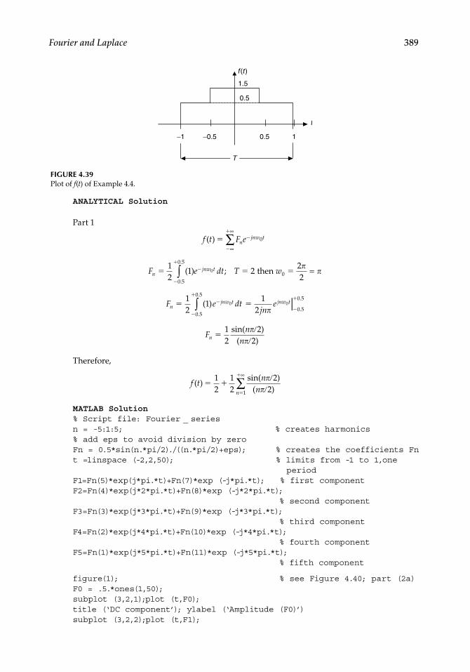
Fourier and Laplace 389
ANALYTICAL Solution
Part 1
f t F en
jnw t( )
∞
∞
∑ 0
F e dt T wn
jnw t 12
1 222
0
0 5
0 5
0( ) ;.
.
∫ = then
F e dt
jnen
jnw t jnw t 1
21
12
0 0
0 5
0 5
0 5
0 5( )
.
.
.
.
∫ |
F
nnn
12
22
sin( )( )
Therefore,
f tn
nn
( )sin( )
( )
12
12
221
∞
∑
MATLAB Solution% Script file: Fourier _ seriesn = -5:1:5; % creates harmonics% add eps to avoid division by zeroFn = 0.5*sin(n.*pi/2)./((n.*pi/2)+eps); % creates the coefficients Fnt =linspace (-2,2,50); % limits from -1 to 1,one periodF1=Fn(5)*exp(j*pi.*t)+Fn(7)*exp (-j*pi.*t); % first componentF2=Fn(4)*exp(j*2*pi.*t)+Fn(8)*exp (-j*2*pi.*t); % second componentF3=Fn(3)*exp(j*3*pi.*t)+Fn(9)*exp (-j*3*pi.*t); % third componentF4=Fn(2)*exp(j*4*pi.*t)+Fn(10)*exp (-j*4*pi.*t); % fourth componentF5=Fn(1)*exp(j*5*pi.*t)+Fn(11)*exp (-j*5*pi.*t); % fifth component
figure(1); % see Figure 4.40; part (2a)F0 = .5.*ones(1,50);subplot (3,2,1);plot (t,F0);title (‘DC component’); ylabel (‘Amplitude (F0)’)subplot (3,2,2);plot (t,F1);
FIGURE 4.39Plot of f(t) of Example 4.4.
f (t )
1.5
−0.5 0.5
0.5
−1 1
T
t
CRC_47760_CH004.indd 389CRC_47760_CH004.indd 389 7/28/2008 12:26:09 PM7/28/2008 12:26:09 PM

390 Practical MATLAB® Applications for Engineers
title (‘Fundamental frequency’); ylabel (‘Amplitude of F1’)subplot (3,2,3); plot (t,F2);title (‘Second harmonic’); ylabel (‘Amplitude of F2’)subplot (3,2,4); plot (t,F3);title (‘Third harmonic’); ylabel (‘Amplitude of F3’); subplot (3,2,5); plot (t,F4);title (‘Fourth harmonic’); ylabel (‘Amplitude of F4’); xlabel (‘time (in sec)’)subplot (3,2,6); plot (t,F5);title (‘Fifth harmonic’); ylabel (‘Amplitude ofF5’); xlabel (‘time (in sec)’)
figure(2); % see Figure 4.41, part (2b) plot(t,F1,t,F2,t,F3,t,F4,t,F5);title(‘Harmonic frequencies of f(t)’)ylabel (‘Amplitude’);xlabel (‘time (in sec)’) ;legend (‘first’,’second’,’third’,’fourth’,’fifth’)
figure(3); % Figure 4.42, part (2c) F0 =1;App1 =F0+F1;App2=App1+F2+F3;App3=App2+F4;App4=App3+F5;subplot(2,2,1);plot(t,App1)title(‘Partial sum of first 2 components (F0+F1)’)ylabel(‘Amplitude’);subplot(2,2,2);plot(t,App2);title(‘Partial sum of first 3 harmonics + DC’)ylabel(‘Amplitude’)subplot(2,2,3);plot(t’,App3);title(‘Partial sum of first 4 harmonics + DC’)xlabel(‘time(in sec)’);ylabel(‘Amplitude’);subplot(2,2,4);plot(t’,App4);title(‘Partial sum of first 5 harmonics + DC’)xlabel(‘time (in sec)’);ylabel(‘Amplitude’)
figure(4) % Figure 4.43, parts (2d) & (2e)Fn(6) =.5;subplot (2,1,1);stem(n.*pi,Fn);grid ontitle(‘line spectrum’);ylabel(‘Amplitude of Fn’)subplot(2,1,2);stem(n.*pi,Fn. 2);grid ontitle(‘power spectrum’);xlabel(‘frequency’);ylabel(‘Magnitude of Fn^2’);disp(‘*********************************’);disp(‘ Verification of Parsevals theorem’);disp(‘*********************************’);Fnsquare=Fn. 2;Pave=sum(Fnsquare); % parts (2f)disp(‘ ’);disp(‘ ’);disp(‘The average power using summations of Fn(coefficients) is:’)disp(Pave);
CRC_47760_CH004.indd 390CRC_47760_CH004.indd 390 7/28/2008 12:26:10 PM7/28/2008 12:26:10 PM

Fourier and Laplace 391
−2 −1 0 1 2
time (in sec)
0.2
−0.2
0
Fifth harmonic
Third harmonic0.5
−0.5−2 −1
0
0 1 2
−2 −1 0 1 2
1
−1
0
Fundamental frequencyDC component
Second harmonic
2
1
−1
0
Am
plitu
de (
FO
)A
mpl
itude
of F
2
Am
plitu
de o
f F3
Am
plitu
de o
f F5
Am
plitu
de o
f F4
Am
plitu
de o
f F1
−2 0 1 2
5
−5
−5
0
−2
−2 −1
−1
−1
0 1
0 1 2
Fourth harmonic5
0
2time (in sec)
× 10−17
× 10−17
FIGURE 4.40Plots of part a of Example 4.4.
disp(‘ ’);syms x;intft = 1/2*int(‘Heaviside(x+.5)’,-.5,.5);Pavesym = vpa(intft);disp(‘ ’);disp(‘*********************************’);disp(‘ ’);disp(‘The average power using integration in time is:’);vpa(intft)disp(‘ ’);disp(‘*********************************’);disp(‘ ’);disp(‘The percentage error is :’); % parts (2g)error = (Pavesym-Pave)*100/Pavesym;disp(error)disp(‘ ’);disp(‘**********************************’);
The script fi le Fourier_series is executed and the results are as follows:
>> Fourier _ series
*************************************************Verification of Parseval’s theorem************************************************* The average power using summation of Fn (coefficients) is: 0.4833*************************************************The average power using integration in time is: ans = .50000000000000000000000000000000*************************************************The percentage error is : 3.3472238873502480061006281175660 **************************************************
CRC_47760_CH004.indd 391CRC_47760_CH004.indd 391 7/28/2008 12:26:10 PM7/28/2008 12:26:10 PM

392 Practical MATLAB® Applications for Engineers
Harmonic frequencies of f(t)
firstsecondthirdfourthfifth
0.8
0.6
0.2
−0.2
−0.4
−0.6
−0.8
0
0.4
Am
plitu
de
−2 −1.5 −1 −0.5 0 0.5 1 1.5 2
time (in sec)
FIGURE 4.41(See color insert following page 374.) Plots of part b of Example 4.4.
Partial sum of first 2 components (F0+F1) Partial sum of first 3 harmonics + DC
Partial sum of first 5 harmonics + DC
2
1
1.5
0.5
0
2
1
1.5
0.5
0
2
1
1.5
0.5
0
Am
plitu
de
Am
plitu
de
−2 −1 0 1 2
Partial sum of first 4 harmonics + DC
2
1.5
0.5
1
0
Am
plitu
de
−2 −1 0 1 2
−2 −1 0 1 2
−2 −1 0 1 2
time (in sec) time (in sec)
Am
plitu
de
FIGURE 4.42Plots of part c of Example 4.4.
CRC_47760_CH004.indd 392CRC_47760_CH004.indd 392 7/28/2008 12:26:10 PM7/28/2008 12:26:10 PM

Fourier and Laplace 393
line spectrum
frequency w (in rad/sec)
0.6
0.4
0.2
0.25
0.2
0.15
0.1
0.05
−0.2
0Am
plitu
de o
f Fn
−20 −15 −10 −5 0 5 10 15 20
power spectrum
0
Mag
nitu
de o
f Fn 2
−20 −15 −10 −5 0 5 10 15 20
frequency w (in rad/sec)
FIGURE 4.43Plots of parts d and e of Example 4.4.
Note that the function f(t) in this example is similar to the function analyzed inExa mple 4.1. The differences are a DC shift in magnitude by 1 and a time shiftby 0.5 s.
Observe that simple shifts change the symmetry conditions of the function f(t), creat-ing new harmonics.
Example 4.5
Create the script fi le Fourier_coeff that returns the fi rst fi ve coeffi cients of the exponential FS (F1, F2, F3, F4, and F5), of the function of Example 4.1, given by
f t
nnw t
n
( ) ( )
2 17
0 odd
sin∑
by using
1. Symbolic techniques 2. Numerical techniques 3. Compare the results of part 1 with part 2
MATLAB Solution% Script file : Fourier _ coeff T = 2;w0 = 2*pi/T; nn =1:5;
CRC_47760_CH004.indd 393CRC_47760_CH004.indd 393 7/28/2008 12:26:10 PM7/28/2008 12:26:10 PM

394 Practical MATLAB® Applications for Engineers
syms coesquare expon t ;for k =1:5expon = exp(-j*k*w0*t);coesquare = .5*int(expon,-.5,.5);Fn = .5*sin(k.*pi/2)./((k.*pi/2)+eps);fn(k) = vpa(Fn);f(k) = vpa(coesquare);enddisp(‘***********************************************************’);disp(‘Coefficients Fn of the exponential Fourier Series’);disp(‘Harmonics Sym. Coeff. ‘);disp(‘***********************************************************’);results1 = [nn’ f’];disp(results1)disp(‘***********************************************************’);disp(‘Harmonics Num. Coeff. ‘);disp(‘***********************************************************’);results2 = [nn’ fn’];disp(results2)disp(‘***********************************************************’);
The script fi le Fourier_coeff is executed and the results are as follows:
>> Fourier _ coeff
************************************************************************Coefficients Fn of the exponential Fourier SeriesHarmonics Sym. Coeff. ************************************************************************ [1, .31830988618379067153776752674503][2, 0][3, -.10610329539459689051258917558168][4, 0][5, .63661977236758134307553505349006e-1]************************************************************************
Harmonics Num. Coeff. ************************************************************************[1, .31830988618379063570529297066969][2, .19490859162596877471531966954150e-16][3, -.10610329539459689707214806730917][4, -.19490859162596877471531966954150e-16][5, .63661977236758135467731278822612e-1]
Note that the symbolic results fully agree with the numerical results. Also note that the magnitude of the error is of the order 10−16.
Example 4.6
Create the script fi le square_time_frq that explores the effects in the frequency domain of changing the τ (tau) of the rectangular periodic wave function shown in Figure 4.44 in the time domain, by plotting their respective spectrums, for the following values of τ = 1, 0.5, 0.25, and 0.125. Discuss the results obtained.
CRC_47760_CH004.indd 394CRC_47760_CH004.indd 394 7/28/2008 12:26:11 PM7/28/2008 12:26:11 PM

Fourier and Laplace 395
ANALYTICAL Solution
The coeffi cients of the exponential FS for f(t) are given by
F
Tn
nn
sin( / )
( / )2
2
where T = 2 and
w n0
22
0
for
MATLAB Solution% Script file: square _ time _ frqecho off;n =-10*pi:pi:10*pi;tau1 =1;T=2;Tx1=tau1/T;Fn1 = Tx1*sin(n*pi*Tx1)./(n*pi*Tx1+eps);Fn1(11)=Tx1;
subplot(2,2,1);stem(n,Fn1);title(‘ spectrum of square wave with tau=1’);axis([-30 30 -.6 .6]);ylabel(‘Amplitude’); xlabel(‘w= n*wo (rad per sec)’);tau2=0.5;T=2;Tx2=tau2/T;Fn2=Tx2*sin(n*pi*Tx2)./(n*pi*Tx2+eps);Fn2(11)=Tx2;subplot(2,2,2);stem(n,Fn2);axis([-30 30 -.3 .3]);title(‘ spectrum of square wave with tau=0.5’);ylabel(‘Amplitude’); xlabel(‘w= n*wo (rad per sec)’);tau3 = 0.25;T=2;Tx3=tau3/T; Fn3=Tx3*sin(n*pi*Tx3)./(n*pi*Tx3+eps);Fn3(11) = Tx3;subplot(2,2,3);stem(n,Fn3);axis([-30 30 -.15 .15]);title(‘ spectrum of square wave with tau=0.25’);xlabel(‘w= n*wo (rad per sec)’);ylabel(‘Amplitude’);tau4 = 0.125;T = 2;Tx4 = tau4/T; Fn4 =Tx4*sin(n*pi*Tx4)./(n*pi*Tx4+eps);Fn4(11) = Tx4;subplot(2,2,4);stem(n,Fn4);axis([-30 30 -.1 .1]);title(‘ spectrum of square wave with tau=0.125’);xlabel(‘w= n*wo (rad per sec)’);ylabel(‘Amplitude’);
−1 1
0.5
f (t )
t
1.0
T
−τ/2 −τ/20
FIGURE 4.44Plots of f(t) of Example 4.6.
CRC_47760_CH004.indd 395CRC_47760_CH004.indd 395 7/28/2008 12:26:11 PM7/28/2008 12:26:11 PM

396 Practical MATLAB® Applications for Engineers
The script fi le square_time_frq is executed and the spectrums of the pulses for τ = 1, 0.5, 0.25, and 0.125 are shown in Figure 4.45.
Note that contracting f(t) in the time domain, from τ = 1 s to τ = 0.125 s (by 1/8) pro-duces an expansion in the frequency domain by a factor of 8, with the magnitude scaled by 1/8, verifying the property f(at) ↔ (1/a)F(w/a).
For example, for τ = 1 s, the estimated bandwidth is 1 rad/s, and the magnitude at w =0 is 0.5. For τ = 0.125 s, the estimated bandwidth is 8 rad/s, and the magnitude at w = 0 is 0.06 (which fully agrees with the theoretical value 0.5/8 = 0.06).
Example 4.7
Let us analyze the periodic triangular function f(t) shown in Figure 4.46, defi ned over a period of T = 1, given by the following trigonometric FS:
f t
nnw t
n
( ) sin( )
1 1
10
∑
where T = 1 and
w
T02
2
The equation for f(t) is given by f(t) = −t + 1, over the range 0 ≤ t ≤ 1 (one period).
spectrum of a square wave with tau=1
spectrum of a square wave with tau=0.25
spectrum of a square wave with tau=0.5
spectrum of a square wave with tau=0.125
0.6
0.4
0.2
0
−0.2
−0.4
−20 0 20 −20 0 20
−20 0 20−20 0 20
w=n*wo (rad per sec.) w=n*wo (rad per sec.)
w=n*wo (rad per sec.)w=n*wo (rad per sec.)
0.3
0.2
0.1
−0.1
−0.2
0
Am
plitu
deA
mpl
itude
0.1
0.05
0
−0.05
−0.1
0.15
0.1
0.05
−0.05
−0.1
0
Am
plitu
deA
mpl
itude
FIGURE 4.45Spectrum plots of Example 4.6.
CRC_47760_CH004.indd 396CRC_47760_CH004.indd 396 7/28/2008 12:26:11 PM7/28/2008 12:26:11 PM

Fourier and Laplace 397
Create the script fi le Fourier_approx that returns the following:
1. The plots of the approximation for f(t) using the fi rst 26, 11, and 4 terms of the trigonometric FS, over the range −3 ≤ t ≤ +3.
2. For each of the approximation plots of part 1, evaluate the values of f(t) at t = 0and 0.1.
3. Plot the four-term trigonometric FS approximation over the range 1 ≤ t ≤ 2, with and without the help of a Hamming window, and observe the effects of the window-ing process.
MATLAB Solution%Script file : Fourier _ approxecho off ;t =−3:0.1:3;x25=0;for n=1:1:25;xn25=1/(pi*n)*sin(2*pi*n*t);
x25=x25+xn25; % sum of 25 termsend;ft26=0.5+x25; % add the DC
figure(1)subplot(3,1,1);plot(t,ft26)title('26 term approximation ')ylabel('Amplitude')x10=0;for n=1:1:10;
xn10=1/(pi*n)*sin(2*pi*n*t);x10=x10+xn10; % sum of 10 terms
end;x3=0;for n=1:1:3;xn3 =1/(pi*n)*sin(2*pi*n*t);x3 = x3+xn3; % sum of 3 termsend;ft4 = 0.5+x3; % add DC ft11 = 0.5+x10; subplot(3,1,2);plot(t,ft11);ylabel('Amplitude');title('11 term approximation ')subplot(3,1,3);plot(t,ft4);ylabel('Amplitude')
0t (s)
f (t )
1
1T=1
FIGURE 4.46Plot of f(t) of Example 4.7.
CRC_47760_CH004.indd 397CRC_47760_CH004.indd 397 7/28/2008 12:26:11 PM7/28/2008 12:26:11 PM

398 Practical MATLAB® Applications for Engineers
xlabel('time (in sec)')title('4 term approximation ')minft26 = min(ft26); maxft26 = max(ft26);minft11 = min(ft11); maxft11 = max(ft11);minft4 = min(ft4);maxft4 = max(ft4)A=[minft26 maxft26];disp(‘******************************************’)disp(' *********R E S U L T S ****************')disp('***********************************************************');disp ('The magnitude of f(t) using 26 terms at t = 0, and t = 0.1 are:');disp (A);B=[minft11 maxft11];C=[minft4 maxft4];disp ('The magnitude of f(t) using 11 terms at t = 0, and t = 0.1 are:');disp (B)disp ('The magnitude of f(t) using 4 terms at t = 0 , and t = 0.1 are:');disp (C);disp('************************************************************');win=hamming(21)
figure(2)subplot(2,1,1); tt=1:.1:2;Ft4=ft4(21:41); F4=ft4(31:41)plot(tt,F4)title('Four term approximation over one cycle');ylabel('Amplitude');subplot(2,1,2)ft4 _ win = Ft4.*win';ttt =1:.1:2, f4 = ft4 _ win(11:21)plot(ttt,f4)title('Four term hamm. window approximation over one cycle');ylabel('Amplitude');xlabel('time (in sec)')
Back at the command window, the script fi le Fourier_ approx is executed and the results are as follows:
>> Fourier _ approx
****************************************** *********R E S U L T S *****************************************************************************The magnitude of f(t) using 26 terms at t=0 , and t=0.1 are: 0.0806 0.9194
The magnitude of f(t) using 11 terms at t=0 , and t=0.1 are: 0.1469 0.8531
The magnitude of f(t) using 4 terms at t=0 , and t=0.1 are: 0.0606 0.9394*************************************************************
Observe that the approximation using four terms is better than the approximation using 26 or 11 terms evaluated at t = 0 and 0.1; but of course not over a larger range (Figure 4.47).
Figure 4.48 shows the fourier trigonometric series expansion improvement over one cycle with and without windowing the partial sum. Observe that the windowing process removes some ripples from the partial sum of the triangular waveform, and the result is a smoother wave.
CRC_47760_CH004.indd 398CRC_47760_CH004.indd 398 7/28/2008 12:26:12 PM7/28/2008 12:26:12 PM

Fourier and Laplace 399
26 term approximation1
0.5
0.5
−3
−3
−2
−2
−1
−1
0
0
1
1
0
0
Am
plitu
deA
mpl
itude
Am
plitu
de
2
2
3
3
−3 −2 −1 0 1 2 3
11 term approximation
4 term approximation
time (in sec)
1
0.5
0
1
FIGURE 4.47Approximation plots of f(t) of Example 4.7.
Four term approximation over one cycle
Four term hamm. window approximation over one cycle
1
0.8
0.4
0.6
0.2
01 1.1 1.2 1.3 1.4 1.5 1.6 1.7 1.8 1.9 2
Am
plitu
deA
mpl
itude
1
0.8
0.6
0.4
0.2
01 1.1 1.2 1.3 1.4 1.5 1.6 1.7 1.8 1.9 2
time (in sec)
FIGURE 4.48Approximation plots of f(t) using four terms of Example 4.7.
CRC_47760_CH004.indd 399CRC_47760_CH004.indd 399 7/28/2008 12:26:12 PM7/28/2008 12:26:12 PM

400 Practical MATLAB® Applications for Engineers
Example 4.8
1. Evaluate by hand the FT (non-periodic) of the rectangular pulse f(t) shown in Fig-ure 4.49 for the following cases τ = 1, 5, and 10 using the transform pairs provided in Table 4.1.
2. Create the script fi le square_FT_num that returns the plots of the FT of part 1 using a numerical approach.
3. Create the script fi le square_FT_sym that returns the magnitude spectrum expres-sions as well as their plots of the FT of part 1 for different τs using the MATLAB symbolic toolbox. Discuss and compare the results obtained.
ANALYTICAL Solution
Part 1
The expression of the FT of f(t) is
f tw
w( ) ↔
sin( )
22
(from Table 4.1)
where τ takes the value of 1, 5, and 10.
MATLAB Solution % Script file: square _ FT _ num % This file returns the plot of the pulse spectrums for the tau’s= 1,5, and 10 echo off; w =-10*pi:0.1:10*pi; F1 = ones(size(w)); F10 = ones(size(w)); tau1=1;tau5 =5;tau10 = 10; F1= sin(w*tau1/2)./(w*tau1/2); F5 = 5*sin(w*tau5/2)./(w*tau5/2);
−τ
0.5
f (t )
t
1.0
−τ/2 0 τ/2 τ
FIGURE 4.49Plot of f(t) of Example 4.8.
CRC_47760_CH004.indd 400CRC_47760_CH004.indd 400 7/28/2008 12:26:12 PM7/28/2008 12:26:12 PM

Fourier and Laplace 401
F10 =10*sin(w*tau10/2)./(w*tau10/2); subplot(3,1,1) plot(w,F1); ylabel(‘Amplitude’); title(‘Spectrum of pulse with tau=1’); axis([-10 10 -1 2]); subplot(3,1,2);plot(w,F5); ylabel(‘Amplitude’); title(‘Spectrum of pulse with tau=5’); axis([-7 8 -4 6]); subplot(3,1,3);plot(w,F10); xlabel(‘frequency w (in rad/sec)’); ylabel(‘Amplitude’); title(‘Spectrum of pulse with tau=10’); axis([-10 10 -4 11]);
The script fi le square_FT_num is executed and the results are as follows (Figure 4.50):
>> square _ FT _ num
frequency w (in rad/sec)
frequency w (in rad/sec)
(Numerical solutions)Spectrum of pulse with τ = 1
2
0
6
4
2
−2
−4
0
1
−1−10
10
5
0
−8 −6
−6
−10 −8 −6 −4 −2 0 2
−4
−4
−2
−2
0
0
2
2
4
4
6
6
8
8
10
Spectrum of pulse τ = 5
Spectrum of pulse τ = 10
frequency w (in rad/sec)4 6 8 10
Am
plitu
deA
mpl
itude
Am
plitu
de
FIGURE 4.50Numerical plots of part 2 of Example 4.8.
CRC_47760_CH004.indd 401CRC_47760_CH004.indd 401 7/28/2008 12:26:12 PM7/28/2008 12:26:12 PM

402 Practical MATLAB® Applications for Engineers
% Script file: square _ FT _ sym % This file returns the expressions and plots for the pulse % spectrums for tau’s= 1,5, and10 syms t w Fw1 = fourier(sym(‘Heaviside(t+1/2)’)- sym(‘Heaviside(t- 1/2)’),t,w); Fw5 = fourier(sym(‘Heaviside(t+2.5)’)- sym(‘Heaviside(t- 2.5)’),t,w); Fw10 = fourier(sym(‘Heaviside(t+5)’)- sym(‘Heaviside(t-5)’),t,w); disp(‘******************************************’) disp(‘ ***********R E S U L T S ************’) disp(‘******************************************’); disp(‘The FT of the rect pulse with tau =1, 5 and 10 are given by:’); Fw1sim = simplify(Fw1) Fw5sim = simplify(Fw5) Fw10sim = simplify(Fw10) disp(‘******************************************’);
figure(1) subplot(3,1,1) ezplot(Fw1sim,[-10 10]) ylabel(‘ Amplitude’) title(‘ Spectrum of the pulse for tau=1.0’) subplot(3,1,2) ezplot(Fw5sim,[-10 10]) axis([-10 10 -4 6]) ylabel(‘ Amplitude’) title(‘ Spectrum of the pulse for tau= 5’) subplot(3,1,3) ezplot(Fw10sim,[-10 10]) axis([-4 4 -6 11]) xlabel(‘frequency w (in rad/sec’), ylabel(‘ Amplitude’) title(‘ Spectrum of the pulse for tau=10’)
The script fi le square_FT_sym is executed and the results are as follows (Figure 4.51):
>> square _ FT _ sym
******************************************************************************************R E S U L T S ******************************************************************************************The FT of the rect pulse with tau =1, 5 and 10 are given by : Fw1sim = 2*sin(1/2*w)/w
Fw5sim = 2.*sin(2.5000000000000000000000000000000*w)/w
Fw10sim = 2*sin(5*w)/w******************************************************************
Observe that the spectrum expressions obtained using the MATLAB symbolic toolbox shown in Figure 4.51 fully agree with the transform of Table 4.1 and the spectrum plots of part 2 shown in Figure 4.52.
CRC_47760_CH004.indd 402CRC_47760_CH004.indd 402 7/28/2008 12:26:12 PM7/28/2008 12:26:12 PM

Fourier and Laplace 403
Example 4.9
Let f(t) = e−2tu(t), evaluate by hand
1. The FT of f(t) ↔ F(w), using Table 4.1 2. The LT of f(t) ↔ F(s), using Table 4.2 3. The analytic expressions of |F(w)| and |F(s)| (magnitude), and angle[F(w)] and
angle[F(s)] (phase) 4. Create the script fi le Fourier_Laplace that returns the following plots:
a f(t) versus t, over −2 ≤ t ≤ 2 b [f(t)]2 versus t (power, assuming R = 1 Ω and f (t) is either a current or a voltage)
5. Evaluate using MATLAB a. Areaof [ ( )] ( )f t f t dt
0 (test the existence of the FT)
b. Energy of [ ( )] ( )f t f t dt 0
2
6. Evaluate the Fourier and Laplace transforms. F(w) and F(s), using the MATLAB symbolic toolbox
7. The symbolic and numerical plots of |F(w)| versus w and |F(s)| versus s
FIGURE 4.51Symbolic plots of part 3 of Example 4.8.
−4
−10 −8 −6 −4 −2 0
Spectrum of the pulse for tau=10
Spectrum of the pulse for tau=5
(Symbolic solution)Spectrum of the pulse for tau=1.0
2 4 6 8 10
−10 −8 −6
1
0.5
0
−4 −2 0 2 4 6 8 10
−3 −2 −1 0 1 2 3 4
10
5
0
−5
frequency w (in rad/sec)
frequency w (in rad/sec)
frequency w (in rad/sec)
Mag
nitu
deM
agni
tude
Mag
nitu
de
4
2
0
−2
−4
6
CRC_47760_CH004.indd 403CRC_47760_CH004.indd 403 7/28/2008 12:26:12 PM7/28/2008 12:26:12 PM

404 Practical MATLAB® Applications for Engineers
ANALYTICAL Solution
Part 1. From Table 4.1, the FT of f(t) = e−2tu(t) ↔ 1/(jw + 2) (transform # 10).Part 2. From Table 4.2, the LT of f(t) = e−2tu(t)↔ 1/(s + 2) (transform # 5).Part 3. The magnitude equations for the Fourier and LTs are
F w
wF s
s( )
( )( )
( )
12
122 2 2 2
The phase equations for the Fourier and LTs are
Phase[F(w)] = −tan−1(w/2) (Fourier)
Phase[F(s)] = −tan−1(s/2) (Laplace)
MATLAB Solution% Script file: Fourier _ Laplacet = -2:0.05:2;ft = exp(-2.*t).*stepfun(t,0);
figure(1)subplot(2,1,1)plot(t,ft)xlabel(‘time (in sec)’);ylabel(‘Amplitude’);axis([-2 2 -.5 1.25]);title(‘exp(-2*t)*u(t) vs. t ‘)subplot(2,1,2)ftsquare = ft. 2; plot(t,ftsquare)xlabel(‘time (in sec)’);ylabel(‘Amplitude’);axis([-2 2 -.5 1.25]);title(‘[exp(-2*t)*u(t)] 2 vs t’)% evaluates integral of exp(-2*t) from 0 to inf.symint = int(‘(exp(-2*t)*Heaviside(t))’,0,inf);symintsq = int(‘(exp(-4*t)*Heaviside(t))’,0,inf);disp(‘******************************’)disp(‘******** R E S U L T S *********’)disp(‘********************************’)disp(‘The int(exp(-2*t)*u(t)) from t=0 to inf is =’)disp(symint)vpa(symint)disp(‘********************************’)disp(‘********************************’)disp(‘The int(exp(-2*t) 2*u(t)) from t=0 to inf is =’)disp(symintsq)vpa(symintsq)disp(‘********************************’)w =-6:0.1:6;Fw =1./sqrt(4+w. 2); % mag [e (-2*t) u(t)] andphase =-atan(w/2); % phase from table of F.T
figure(2)subplot(2,2,1);plot(w,Fw)xlabel(‘frequency w’);ylabel(‘Magnitude of F(w)’)title(‘Magnitude spectrum/Fourier’);
CRC_47760_CH004.indd 404CRC_47760_CH004.indd 404 7/28/2008 12:26:13 PM7/28/2008 12:26:13 PM

Fourier and Laplace 405
axis([-5 5 0 0.6])subplot(2,2,2);plot(w,phase*180/pi)xlabel(‘frequency w’);ylabel(‘Angle in degrees’)title(‘Phase spectrum/Fourier’);a = [1]; % F(s) = 1/(s+2)b = [1 2]; H = freqs(a,b,w);mag = abs(H);ang = angle(H);degrees = ang*180/pi;subplot(2,2,3);plot(w,mag)xlabel(‘frequency s’);ylabel(‘Magnitude of F(s)’)title(‘Magnitude spectrum/Laplace’);axis([-5 5 0.1 0.6])subplot(2,2,4);plot(w,degrees)xlabel(‘frequency s’);ylabel(‘Angle in degrees’)title(‘Phase spectrum/Laplace’);
figure(3)% Fourier transform using the symbolic toolboxsyms v;disp(‘********************************’)disp(‘The sym Fourier transform ‘) disp(‘of(exp(-2*t)*u(t)) is=’)FT= fourier(exp(-2*v)*sym(‘Heaviside(v)’)) disp(‘********************************’)% Laplace transform using symbolic toolboxdisp(‘********************************’)disp(‘The sym Laplace transform ‘) disp(‘of(exp(-2*t)*u(t)) is=’)LT=laplace(exp(-2*v)*sym(‘Heaviside(v)’)) disp(‘********************************’)subplot(2,1,1);ezplot(abs(FT));title(‘sym Fourier transf of(exp(-2*t)*u(t))’)ylabel(‘Magnitude of F(w)’);xlabel(‘frequency w’);subplot(2,1,2);ezplot(abs(LT));title(‘sym Laplace transf of(exp(-2*t)*u(t))’)ylabel(‘Magnitude of F(s)’);xlabel(‘frequency s’);axis([-4 0 0 45])
The script fi le Fourier_Laplace is executed and the results are as follows (Figures 4.52 through 4.54):
>> Fourier _ Laplace
**************************************************** R E S U L T S *****************************************************The int(exp(-2*t)*u(t)) from t=0 to inf is = 1/2
ans = .50000000000000000000000000000000
CRC_47760_CH004.indd 405CRC_47760_CH004.indd 405 7/28/2008 12:26:13 PM7/28/2008 12:26:13 PM

406 Practical MATLAB® Applications for Engineers
**********************************************************************************The int(exp(-2*t) 2*u(t)) from t=0 to inf is = 1/4
ans = .25000000000000000000000000000000*****************************************
*****************************************The sym Fourier transform of(exp(-2*t)*u(t)) is= FT = 1/(2+i*w) *****************************************
*****************************************The sym Laplace transform of(exp(-2*t)*u(t) is= LT = 1/(s+2)*****************************************
−2 −1.5 −1 −0.5 0 0.5 1 1.5 2time (in sec)
−2 −1.5 −1 −0.5 0 0.5 1 1.5 2time (in sec)
−0.5
0
0.5
1
−0.5
0
0.5
1
Am
plitu
deA
mpl
itude
exp(-2*t)*u(t) versus t
[exp(-2*t)*u(t)]2 versus t
FIGURE 4.52Symbolic plots of part 4 of Example 4.9.
CRC_47760_CH004.indd 406CRC_47760_CH004.indd 406 7/28/2008 12:26:13 PM7/28/2008 12:26:13 PM

Fourier and Laplace 407
−5 00.1
0.2
0.3
0.4
0.5
0.6
5
−5 00
0.2
0.4
5 −10−100
−50
50
100
−5
frequency s
Mag
nitu
de o
f F(w
)M
agni
tude
of F
(s)
Magnitude spectrum/Fourier
Magnitude spectrum/Laplace
Phase spectrum/Fourier
Phase spectrum/Laplace
0 5 10
−5 0 5 10
0
−10−100
−50
50
100
0
Ang
le in
deg
rees
Ang
le in
deg
rees
frequency w
frequency w
frequency s
FIGURE 4.53Numerical plots of F(w) and F(s) of part 7 of Example 4.9.
FIGURE 4.54Symbolic plots of F(w) and F(s) of part 7 of Example 4.9.
0.5
0.4
0.3
0.2
−6 −4
−4 −3.5 −3 −2.5 −2 −1.5 −1 −0.5
−2 0 2 4 6
0
40
30
20
10
0
Mag
nitu
de o
f F(s
)M
agni
tude
of F
(w)
sym Fourier transf of (exp(-2*t)*u(t))
sym Laplace transf of (exp(-2*t)*u(t))
frequency s
frequency w
CRC_47760_CH004.indd 407CRC_47760_CH004.indd 407 7/28/2008 12:26:13 PM7/28/2008 12:26:13 PM

408 Practical MATLAB® Applications for Engineers
Example 4.10
Analyze by hand and using MATLAB (include pretty) the block box system diagram shown in Figure 4.55, and obtain
a. Analytical expressions of i. X(w) ii. H(w) iii. Y(w) iv. y(t)
b. Create the script fi le syst_anal that returns the following plots: i. X(w) versus w (numerical) ii. H(w) versus w (numerical) iii. Y(w) versus w (numerical) iv. |H(w)| versus w, and verify that its spectrum consists of two impulses, located at
w = ±3 rad/s v. x(t) versus t, h(t) versus t, and y(t) versus t vi. X(w) versus w (symbolic) vii. Y(w) versus w (symbolic)
ANALYTICAL Solution
Part a: From Table 4.1, the following transforms are obtained:
ℑ
ℑ
[ ( ) ( )] ( )( )
( )
[ ( ) ] ( )
x t t X ww
w
h t e H ww
Y
t
pulsin
2
69
32
(( ) ( ) ( )sin( )
( ) ( )
( ) ( ) ( )
w X w H ww
w w
y t x t h t
⋅⋅
⊗
1292
where
y t x h t d x t h t( ) ( ) ( ) ( ) ( )
−∞
∞
∫ (convolution of with )
MATLAB Solution[part(b)]% Script file: syst _ analecho off;w =-2*pi:0.01:2*pi;w =w+eps;
h(t ) = e −3[t]
−π +π
x (t )
y (t )t1
FIGURE 4.55Block box system diagram of Example 4.10.
CRC_47760_CH004.indd 408CRC_47760_CH004.indd 408 7/28/2008 12:26:13 PM7/28/2008 12:26:13 PM

Fourier and Laplace 409
xw =2*pi*sin(w*pi)./(w*pi); % FT of x(t) from Table 4.1,transf.#3% H(w) = 6/(w^2+9); % FT of h(t) from Table 4.1,transf.#13a = [6];b = [1 0 9];Hw = freqs(a,b,w);magxw = abs(xw);magHw = abs(Hw);yw = magxw.*magHw;
figure(1)subplot(3,1,1);plot(w,magxw);ylabel(‘Magnitude’);axis([-6 6 0 8]);title(‘ X(w) vs.w’);xlabel(‘frequency w(rad/sec)’);subplot(3,1,2);plot(w,magHw);axis([-6 6 0 8]);ylabel(‘Magnitude’);title(‘ H(w) vs.w’);xlabel(‘frequency w(rad/sec)’);magyw=magxw.*magHw;subplot(3,1,3)plot(w,magyw);axis([-6 6 0 5]);ylabel(‘Magnitude’);title(‘ Y(w) vs.w’);xlabel(‘frequency w(rad/sec)’);
figure(2)plot(w,magHw);title(‘ H(w) vs. w (showing impulses)’);ylabel(‘Magnitude’);xlabel(‘fequency w (rad/sec)’)magyw=magxw.*magHw;%time domain analysis
figure(3)t=-5:.1:5;xt=[zeros(1,20) ones(1,61) zeros(1,20)];ht=exp(-3.*abs(t));hut=[zeros(1,50) ones(1,51)];htt=ht.*hut;conxh=conv(xt,ht);tt=-10:.1:10;subplot(3,1,1)plot(t,xt);axis([-5 5 0 1.5])title(‘x(t) vs. t’);ylabel(‘Amplitude’);xlabel(‘time (in sec)’)subplot(3,1,2)plot(t,ht);title(‘h(t) vs. t’);axis([-2 2 0 1.5])ylabel(‘Amplitude’);xlabel(‘time (in sec)’);subplot(3,1,3)plot(tt,conxh);title(‘y(t) vs. t’);ylabel(‘Amplitude’);xlabel(‘time (in sec)’)
% Symbolic evaluationssyms x;FTx = fourier(sym(‘Heaviside(x-pi)’)-sym(‘Heaviside(x+pi)’));
CRC_47760_CH004.indd 409CRC_47760_CH004.indd 409 7/28/2008 12:26:14 PM7/28/2008 12:26:14 PM

410 Practical MATLAB® Applications for Engineers
FTxsym =simplify(FTx) ; % X(w)FTh = fourier(exp(- 3*x)*sym(‘Heaviside(x)’)+ exp(3*x)*sym(‘Heaviside(-x)’)); FTy = FTx*FTh;FTysym=simplify(FTy) ; %Y(w)Disp(‘*****************************************************’)disp(‘******* S y m b o l i c **** R e s u l t s*********’)disp(‘ ‘)disp(‘The Fourier Transf. of x(t) is:’)disp(FTxsym)pretty(FTxsym)disp(‘The Fourier Transf. of h(t) is:’)disp(FTh)pretty(FTh)disp(‘The Fourier Transf. of y(t) is:’)disp(FTysym)pretty(FTysym)disp(‘*****************************************************’)
figure(4)subplot(2,1,1)ezplot(abs(FTxsym));title(‘Symbolic plot of the Fourier Transf. of X(t) vs. w ‘)ylabel(‘Magnitude’);xlabel(‘ frequency (in rad/sec)’);axis([-6 6 0 6])subplot(2,1,2)ezplot(abs(FTysym),[-6 6]);title(‘Symbolic plot of the Fourier Transf. of Y(t) vs. w ‘)ylabel(‘Magnitude’);xlabel(‘frequency w (in rad/sec)’); axis([-6 6 0 5]);
The script fi le syst_anal is executed and the results are as follows (Figures 4.56 through 4.59):
>> syst _ anal
************************************************************* S y m b o l i c **** R e s u l t s*********
The Fourier Transf. of x(t) is: -2*sin(pi*w)/w sin(pi w)-2 --------- w
The Fourier Transf. of h(t) is: 1/(3+i*w)+1/(3-i*w) 1 1 ------- + -------- 3 + i w 3 - i w
The Fourier Transf. of y(t) is: 12*sin(pi*w)/w/(3+i*w)/(-3+i*w) sin(pi w) 12 ----------------------- w (3 + i w) (-3 + i w)*****************************************************
CRC_47760_CH004.indd 410CRC_47760_CH004.indd 410 7/28/2008 12:26:14 PM7/28/2008 12:26:14 PM

Fourier and Laplace 411
FIGURE 4.56Plots of X(w), H(w), and Y(w) of Example 4.10.
−6 −4 −2 0 2 4 6
−6 −4 −2 0 2 4 6
−6 −4 −2 0 2 4 6
frequency w(rad/sec)
frequency w(rad/sec)
frequency w(rad/sec)
8
6
4
2
0
Mag
nitu
de
8
6
4
2
0
Mag
nitu
deM
agni
tude
4
2
0
X(w) versus w
H(w) versus w
Y(w) versus w
FIGURE 4.57Plot of H(w) of Example 4.10.
350
300
250
200
150
100
50
0−8 −6 −4 −2 0 2 4 6 8
frequency w (rad/sec)
H(w) versus w (showing impulses)
Mag
nitu
de
CRC_47760_CH004.indd 411CRC_47760_CH004.indd 411 7/28/2008 12:26:14 PM7/28/2008 12:26:14 PM

412 Practical MATLAB® Applications for Engineers
−10 −8 −6 −4 −2
−2 −1.5 −1
−5 −4 −3 −2 −1
−0.5 0 0.5
0 2 4 6 8 100
5
10
y(t) versus t
1 1.5 20
0.5
1
1.5
0 1 2 3 4 5
1.5
1
0.5
0
Am
plitu
deA
mpl
itude
Am
plitu
dex(t) versus t
h(t) versus t
time (in sec)
time (in sec)
time (in sec)
FIGURE 4.58Plots of x(t), h(t), and y(t) of Example 4.10.
6
4
2
0−6 −4 −2 0 2 4 6
Symbolic plot of the Fourier Transf. of x(t) versus w
Symbolic plot of the Fourier Transf. of y(t) versus w
frequency (in rad/sec)
−6 −4 −2 0 2 4 6frequency w (in rad/sec)
Mag
nitu
deM
agni
tude
5
4
3
2
1
0
FIGURE 4.59Symbolic plots of X(w) and Y(w) of Example 4.10.
CRC_47760_CH004.indd 412CRC_47760_CH004.indd 412 7/28/2008 12:26:14 PM7/28/2008 12:26:14 PM

Fourier and Laplace 413
h (t ) = 0.5e−0.5tu(t )x(t) = 5cost + 15cos15t y (t )
FIGURE 4.60Block box system diagram of Example 4.11.
Example 4.11
Let us analyze the block system diagram shown in Figure 4.60, by creating the script fi le analysis that returns the following plots using numerical techniques:
1. x(t) versus t and |X(w)| versus w 2. h(t) versus t, |H(w)| versus w (magnitude), and phase of [H(w)] versus w 3. y(t) versus t, |Y(w)| versus w, and phase [Y(w)] versus w
MATLAB Solution% Script file: analysist = -5:0.01:5;xt = 5*cos(t)+15*cos(15*t);subplot(3,2,1),plot(t,xt)title(‘ x(t) vs. t’) ,ylabel(‘ Amplitude’)w =-30:1:30;xw =pi*[zeros(1,15) 15 zeros(1,13) 5 0 5 zeros(1,13) 15 zeros(1,15)]; % spectrum of x(t)%from Table 4.1 transform 6subplot(3,2,2),stem(w,xw)title(‘X(w) vs. w ‘);ylabel(‘ Magnitude’);axis([-30 30 -5 60]);to = 0;ut = stepfun(t,to);h = 0.5*exp(-0.5*t);ht = h.*ut;subplot (3,2,3);plot (t,ht);title (‘ h(t) vs. t’);ylabel(‘Amplitude’)axis([-3 5 -.5 1]);% FT of h(t) is 0.5/(s+0.5), s=jw;% from Table 4.1 a = [0.5];b = [1 0.5];Hw = freqs(a,b,w);magHw = abs(Hw);phase = angle(Hw);subplot(3,2,4),plotyy(w,magHw,w,phase)title(‘Magnitude & phase of H(w)’);% Convolution of x(t) and h(t)yt = conv(xt,ht); lengyt = length(yt)-1;n = [0:1:lengyt]-[5*ones(1,lengyt+1)];subplot(3,2,5),plot(n/100,yt/100)
CRC_47760_CH004.indd 413CRC_47760_CH004.indd 413 7/28/2008 12:26:14 PM7/28/2008 12:26:14 PM

414 Practical MATLAB® Applications for Engineers
FIGURE 4.61Time and frequency plots of the signals of the block box system of Example 4.11.
20
−20−5
−2
1
5
0
0
−5
5
0
0 2
5 10time
15 −40
−10
−20−2
4
1
0.5
0
0.5
−0.5
h(t) versus t
y(t) versus t
x(t) versus t X(w) versus w
0
0
2
0
5
20 40
−40 −20
−20
00
20
0
0
60
40
20
20
40
Phase
−2
0
2
Phase
phase
phase
frequency w (in rad/sec)
Magnitude & phase of Y(w)
Magnitude & phase of H(w)
magnitude
magnitude
Am
plitu
deA
mpl
itude
Am
plitu
de
Mag
nitu
deM
agni
tude
Mag
nitu
de
xlabel(‘time’),title(‘ y(t) vs. t’);ylabel(‘Amplitude’)yw = magHw.*xw;axis([5 15 -5 5])subplot(3,2,6),plotyy(w,yw,w,phase);xlabel(‘frequency w (in rad/sec)’), title(‘Magnitude & phase of Y(w)’);
The script fi le analysis is executed and the results are as follows (Figure 4.61):
TIME DOMAIN FREQUENCY DOMAIN************************************************************
Example 4.12
Given the circuit shown in Figure 4.62,
1. Determine by hand the system transfer function H(s) = V0(s)/Vi(s) 2. Obtain an expression for v0(t), from part 1, where vi(t) = u(t) 3. Use MATLAB to obtain plots of v0(t) versus t, using an analytical and symbolic
approach
CRC_47760_CH004.indd 414CRC_47760_CH004.indd 414 7/28/2008 12:26:14 PM7/28/2008 12:26:14 PM

Fourier and Laplace 415
FIGURE 4.62Circuit diagram of Example 4.12.
C = 1F
R = 1 Ω V0(t )
Vi(t ) Vi(s)
V0(s)
ANALYTICAL Solution
Part 1
H s
V sV s
RR sC
ssi
( )( )( ) ( / )
0
1 1
Part 2
V s
sV s
sv t V s e u ti
t( ) ( ) ( ) [ ( )] ( ) ( ) 1 1
140 0
10+
£ from Table .2
Part 3
MATLAB Solution% Script file :analysis _ RC t =-1:0.1:8;t0 = 0;ut =stepfun(t,t0);vo =exp(-t);vot =vo.*ut;subplot(2,1,1);plot(t,vot,t,vot,’o’);title(‘vo(t) vs. t,numerical solution’);xlabel(‘time(sec)’);ylabel(‘ Amplitude (volts)’);axis([-1 5 -.5 1.3]);syms s x Hs = s/(s+1);Vis =1/s;Vos = Hs*Vis;vot = ilaplace(Vos);subplot(2,1,2);ezplot(vot);title(‘vo(t) vs. t, symbolic solution’);ylabel(‘ Amplitude (volts)’);xlabel(‘time(sec)’);axis([0 5 -.5 1.3]);
The script fi le analysis_RC is executed and the results are shown in Figure 4.63.
CRC_47760_CH004.indd 415CRC_47760_CH004.indd 415 7/28/2008 12:26:15 PM7/28/2008 12:26:15 PM

416 Practical MATLAB® Applications for Engineers
Example 4.13
The switch sw shown in the circuit diagram of Figure 4.64 has been opened for a long time. At t = a = 0, the sw closes and remains closed for t ≥ 0. Assume that all the initial conditions are zero. Determine by hand an expression for i(t). Create the script fi le analy-sis_RLC that returns i(t) using the LT, and obtain plots of i(t) versus t for t ≥ 0, using a numerical and symbolic approach.
Also obtain the symbolic expression fot i(t), for t ≥ 0, using Laplace for the case when the sw closes at t = a = 1.
ANALYTICAL Solution
Z s R sLsC
( ) ( ) 1
total impedence
FIGURE 4.64Circuit diagram of Example 4.13.
50 V
R = 2 Ω
L = 1 H
C = 0.1 F
sw closes at t = a
i(t )
0
0
0 1 2 3 4 5
0.5 1
1
0.5
−0.5
0
1
0.5
−0.5−1
2 3 4 52.5 3.5 4.51.5
time (sec)
time (sec)
v0(t) versus t (symbolic solution)
v0(t) versus t (numerical solution)
Am
plitu
de (
volts
)A
mpl
itude
(vo
lts)
FIGURE 4.63Numerical and symbolic plots of v0(t) of Example 4.12.
CRC_47760_CH004.indd 416CRC_47760_CH004.indd 416 7/28/2008 12:26:15 PM7/28/2008 12:26:15 PM

Fourier and Laplace 417
Y sZ s
Y sR sL sC
ss s
ss
I sV sZ
( )( )
( )( / ) ( )
( )( )
1 11 2 10 1 32 2 2
(( )( ) ( )
sV s Y s
Since
V s u t
s( ) [ ( )] £ 50
50
then
I ss
ss s
i t I s e t
( )( ) ( )
( ) [( ( )] si
501 3
503
31 3
503
2 2 2 2
1
⋅
⋅£ nn( ) ( )3t u t⋅
MATLAB Solution% Script file : analysis _ RLCt =-1:0.1:8;t0=0;u = stepfun(t,t0);it = 50/3*exp(-t).*sin(3*t).*u;subplot(2,1,1)plot(t,it);title(‘i(t) vs t (numeric solution)’)xlabel(‘time(sec)’)ylabel(‘Amplitude (amps)’)axis([0 6 -4 11])syms s zszs = 2+s+(1/(s*.1));vs = 50/s;ILs = vs/zs;IL = ilaplace(ILs);disp(‘*******************************************’)disp(‘ **** symbolic result (sw closes at t=0)*****’)disp(‘The current i(t) (in amps) is :’)simIL = simplify(IL);disp(simIL)subplot(2,1,2)ezplot(simIL)title(‘i(t) vs. t (symbolic solution)’)axis([0 6 -4 11])xlabel(‘time(sec)’)ylabel(‘Amplitude (amps)’)t0=1; IL = ilaplace((ILs)*exp(-s)); %sw closes at t=1disp(‘******* *symbolic result(sw closes at t=1) *****’)disp(‘The current i(t) (in amps) is given by :’)simIL = simplify(IL);disp(simIL)disp(‘***************************************’)
CRC_47760_CH004.indd 417CRC_47760_CH004.indd 417 7/28/2008 12:26:15 PM7/28/2008 12:26:15 PM

418 Practical MATLAB® Applications for Engineers
The script fi le analysis_RLC is executed and the results are as follows (Figure 4.65):
>> analysis _ RLC
********************************************************* symbolic result (sw closes at t =0)*********** The current i(t) (in amps) is given by : 25/3*i*(-exp((-1+3*i)*t)+exp((-1-3*i)*t))********** symbolic result (sw closes at t =1)***** The current i(t) (in amps) is : 50/3*Heaviside(t-1)*exp(-t+1)*sin(3*t-3)***************************************
0
0
5
10
1 2 3 4 5 6time (sec)
0 1 2 3 4 5 6time (sec)
Am
plitu
de (
amps
)
0
5
10
Am
plitu
de (
amps
)
i(t) versus t (symbolic solution)
i(t) versus t (numeric solution)
FIGURE 4.65Numerical and symbolic plot of i(t) of Example 4.13.
Example 4.14
Create the script fi le repeat_RLC that returns the current i(t) of Example 4.13, shown in Figure 4.64, for t ≥ 0, assuming that the sw closes at t = 0, for the following voltage source:
1. A unit impulse (use the impulse function) 2. A unit step (use the step function)
CRC_47760_CH004.indd 418CRC_47760_CH004.indd 418 7/28/2008 12:26:16 PM7/28/2008 12:26:16 PM

Fourier and Laplace 419
ANALYTICAL Solution
Recall that
I s V s
ss s
( ) ( )
⋅2 2 10
where the applied voltage is either δ (t) or u(t), with a LT of 1 or 1/s (Table 4.2).
MATLAB Solution% Script file : repeat _ RLCnum = [0 1 0];den = [1 2 10];t = 0:0.1:8*pi;impres= impulse(num,den,t);stepres= step(num,den,t);subplot(2,1,1)plot(t,impres);title(‘Impulse response ‘);ylabel(‘magnitude’);axis([0 5 -1 1]);subplot(2,1,2)plot(t,stepres);title(‘Step response ‘);xlabel(‘time(sec)’);ylabel(‘magnitude’);axis([0 5 -.1 .3])
The script fi le repeat_RLC is executed and the results are shown in Figure 4.66.
0
0
0.1
0.2
0.3
1 2 3 4 51.5 2.5 3.5 4.50.5
0
0
1
1
2 3 4 51.5 2.5 3.5 4.50.5
0.5
−0.1
−0.5
−1
Am
plitu
deA
mpl
itude
time (sec)
Step response
Impulse response
FIGURE 4.66Impulse and step plots of Example 4.14.
CRC_47760_CH004.indd 419CRC_47760_CH004.indd 419 7/28/2008 12:26:16 PM7/28/2008 12:26:16 PM

420 Practical MATLAB® Applications for Engineers
Example 4.15
The switch in the circuit diagram of Figure 4.67 is closed for a long time. At t = 0, the switch is opened and remains opened for t ≥ 0. Analyze by hand the given circuit using the LT and obtain analytical expressions for
v(t), ir(t), ic(t), il(t) for t ≥ 0
Create the script MATLAB fi le RLC_parallel that returns the plots of the analytical results as well as the symbolic (Laplace) plots of v(t), ir(t), ic(t), il(t), over the range−2 ≤ t ≤ 5, and observe that both solutions are identical.
3 Aswitch opens at t = 0
R = 20 Ω
C = 1/40 FL = 5 HV (s)
FIGURE 4.67Circuit diagram of Example 4.15.
ANALYTICAL Solution
The nodal equation yields
V s V s
ssV s
st
( ) ( ) ( )20 5 40
3 for 0
then
V ss
ss
V ss s
s s
V s s s
( )
( )
( )(
120
15 40
3
2 840
3
2
2
2
88 120) , ( ) solving for voltage V s
V s
s s s( )
( )
1202 2 22 8
1207
71 7
⋅
CRC_47760_CH004.indd 420CRC_47760_CH004.indd 420 7/28/2008 12:26:16 PM7/28/2008 12:26:16 PM

Fourier and Laplace 421
Then from Table 4.2
v t e t u tt( ) sin( ) ( )
1207
7⋅ ⋅
and therefore,
i tv tR
e t u t
i t Cdv t
dtddt
e
Rt
Ct
( )( )
sin( ) ( )
( )( )
67
7
140
1207
⋅
⋅ ssin( ) ( )
( ) cos( ) ( )
7
37
7 7 737
t u t
i t e t t e eCt t t
sin 77 7 7
3
367
cos ( )( ) sin( )
( ) ( ) ( )
( )
t t
i t i t i t
i t e
L R C
Lt
−
u t
7cos( 7 ) sin( 7 ) sin( ) ( ) ( )737
t u t e u tt − t t
MATLAB Solution% Script file: RLC _ parallelt =-2:0.1:5;t0 =0;u = stepfun(t,t0);vt =120/sqrt(7).*exp(-t).*sin(sqrt(7).*t).*u ;
figure(1)subplot(2,2,1);plot(t,vt);title(‘ v(t) vs.t (analytical)’);ylabel(‘Amplitude (volts)’)ir = 6/sqrt(7)*exp(-t).*sin(sqrt(7).*t).*u;subplot(2,2,2);plot(t,ir);title(‘ ir(t) vs.t (analytical)’);ylabel(‘ Amplitude (amps)’)ic=3/sqrt(7).*exp(-t).*(sqrt(7).*cos(sqrt(7).*t)- sin(sqrt(7).*t)).*u;subplot(2,2,3);plot(t,ic);title(‘ ic(t) vs.t (analytical)’);ylabel(‘Amplitude (amps)’);xlabel(‘time(sec)’);subplot(2,2,4);il = 3*ones(1,71)-ir-ic ;plot(t,il);title(‘il(t) vs.t (analytical)’);ylabel(‘Amplitude (amps)’) ;xlabel(‘time (sec)’);
figure(2)subplot(2,2,1)num = [0 0 120];den = [1 2 8];vti = impulse(num,den,t);vti=[zeros(1,20) vti’];plot(t,vti);title(‘ v(t) vs. t (sym. Laplace)’);
CRC_47760_CH004.indd 421CRC_47760_CH004.indd 421 7/28/2008 12:26:17 PM7/28/2008 12:26:17 PM

422 Practical MATLAB® Applications for Engineers
FIGURE 4.68Plots of the analytical solutions of Example 4.15.
30
20
10
−10
−2
−1
−2
0
0 2 4 6
−2 0
0
1
2
3
1
0
2
3
4
2 4 6 −2 0 2 4 6
−2−0.5
0.5
0
0
1
1.5
2 4 6
time (sec) time (sec)
Am
plitu
de (
amps
)A
mpl
itude
(vo
lts)
Am
plitu
de (
amps
)A
mpl
itude
(am
ps)
v(t) versus t (analytical) ir(t) versus t (analytical)
il(t) versus t (analytical)ic(t) versus t (analytical)
ylabel(‘Amplitude (volts)’)subplot(2,2,2)numr = [0 0 6];%IR=6/s^2+s+8;denr = [1 2 8];ir = impulse(numr,denr,t);ir = [zeros(1,20) ir’];plot(t,ir);title(‘ ir(t) vs. t (sym. Laplace)’);ylabel(‘Amplitude (amps)’)subplot(2,2,3)numc =[0 3 0];%IC=3s/(s^2+2s+8);denc = [1 2 8];ic = impulse(numc,denc,t);ic=[zeros(1,20) ic’];plot(t,ic);title(‘ ic(t) vs. t (sym. Laplace)’);ylabel(‘Amplitude (amps)’);xlabel(‘time(sec)’);subplot(2,2,4)numl = [0 0 0 120];denl = [5 10 40 0];%IL(s)=120/(5s^3+10s^2+40s);il =impulse(numl,denl,t);il=[3*ones(1,20) il’];plot(t,il);title(‘ il(t) vs. t (sym. Laplace)’);ylabel(‘Amplitude (amps)’) ;xlabel(‘time (sec)’);
The script fi le RLC_parallel is executed and the results are shown in Figures 4.68and 4.69.
Note that the analytical solutions fully agree with the symbolic solutions.
CRC_47760_CH004.indd 422CRC_47760_CH004.indd 422 7/28/2008 12:26:17 PM7/28/2008 12:26:17 PM
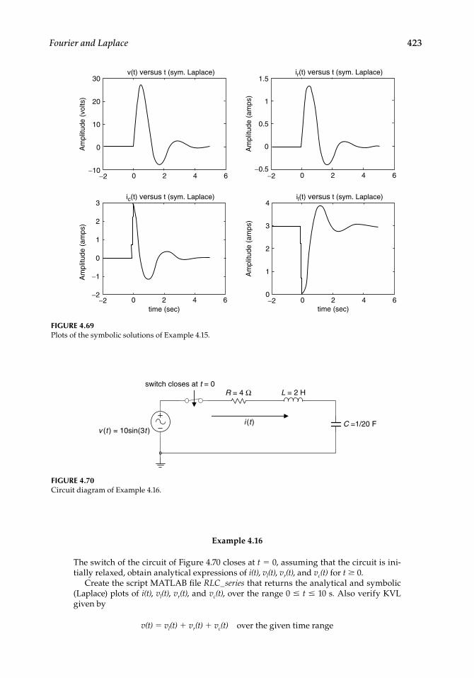
Fourier and Laplace 423
30
20
10
−10
−2
−1
−2
0
0 2 4 6
−2 0
0
1
2
3
1
0
2
3
4
2 4 6 −2 0 2 4 6
−2−0.5
0.5
0
0
1
1.5
2 4 6
time (sec) time (sec)
Am
plitu
de (
amps
)A
mpl
itude
(vo
lts)
Am
plitu
de (
amps
)A
mpl
itude
(am
ps)
v(t) versus t (sym. Laplace) ir(t) versus t (sym. Laplace)
il(t) versus t (sym. Laplace)ic(t) versus t (sym. Laplace)
FIGURE 4.69Plots of the symbolic solutions of Example 4.15.
Example 4.16
The switch of the circuit of Figure 4.70 closes at t = 0, assuming that the circuit is ini-tially relaxed, obtain analytical expressions of i(t), vl(t), vr(t), and vc(t) for t ≥ 0.
Create the script MATLAB fi le RLC_series that returns the analytical and symbolic (Laplace) plots of i(t), vl(t), vr(t), and vc(t), over the range 0 ≤ t ≤ 10 s. Also verify KVL given by
v(t) = vl(t) + vr(t) + vc(t) over the given time range
v (t ) = 10sin(3t )
R = 4 Ω L = 2 H
C =1/20 F
switch closes at t = 0
i (t)
FIGURE 4.70Circuit diagram of Example 4.16.
CRC_47760_CH004.indd 423CRC_47760_CH004.indd 423 7/28/2008 12:26:17 PM7/28/2008 12:26:17 PM
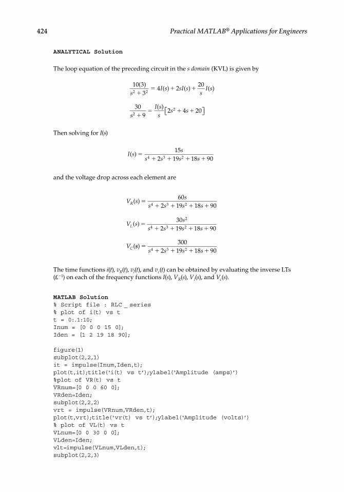
424 Practical MATLAB® Applications for Engineers
ANALYTICAL Solution
The loop equation of the preceding circuit in the s domain (KVL) is given by
10 33
4 220
309
2 4 20
2 2
22
( )( ) ( ) ( )
( )
sI s sI s
sI s
sI s
ss s
Then solving for I(s)
I s
ss s s s
( )
152 19 18 904 3 2
and the voltage drop across each element are
V ss
s s s s
V ss
s s s s
V
R
L
C
( )
( )
(
602 19 18 90
302 19 18 90
4 3 2
2
4 3 2
sss s s s
)
3002 19 18 904 3 2
The time functions i(t), vR(t), vl(t), and vc(t) can be obtained by evaluating the inverse LTs (£−1) on each of the frequency functions I(s), VR(s), Vl(s), and Vc(s).
MATLAB Solution% Script file : RLC _ series% plot of i(t) vs tt = 0:.1:10;Inum = [0 0 0 15 0];Iden = [1 2 19 18 90];
figure(1)subplot(2,2,1)it = impulse(Inum,Iden,t);plot(t,it);title(‘i(t) vs t’);ylabel(‘Amplitude (amps)’)%plot of VR(t) vs tVRnum=[0 0 0 60 0];VRden=Iden;subplot(2,2,2)vrt = impulse(VRnum,VRden,t);plot(t,vrt);title(‘vr(t) vs t’);ylabel(‘Amplitude (volts)’)% plot of VL(t) vs tVLnum=[0 0 30 0 0];VLden=Iden;vlt=impulse(VLnum,VLden,t);subplot(2,2,3)
CRC_47760_CH004.indd 424CRC_47760_CH004.indd 424 7/28/2008 12:26:17 PM7/28/2008 12:26:17 PM

Fourier and Laplace 425
0
0
2
4
−4
−10
−20
−2
5 10 0
20
10
10
0
−10
−20
20
10
0
0 5
0
5
10
−10
−5
5 10
Am
plitu
de (
amps
)
Am
plitu
de (
volts
)A
mpl
itude
(vo
lts)
Am
plitu
de (
volts
)
time (sec)100 5
time (sec)
vl(t) versus t vc(t) versus t
vr(t) versus ti(t) versus t
FIGURE 4.71Plots of i(t), vl(t), vr(t), and vc(t) of Example 4.16.
plot(t,vlt);title(‘vl(t) vs t’);ylabel(‘Amplitude (volts)’);xlabel(‘time (sec)’)%plot of VC(t) vs tVCnum = [0 0 0 0 300];VCden = [1 2 19 18 90];vct = impulse(VCnum,VCden,t);subplot(2,2,4)plot(t,vct);title(‘vc(t) vs t’);ylabel(‘Amplitude (volts)’);xlabel(‘time (sec)’)
figure(2)subplot(2,1,1)plot(t,it,t,vrt,t,vlt,t,vct)title(‘Plots of: i(t) vs.t, vr(t) vs.t, vl(t)vs.t, and vc(t) vs.t’)axis([0,5,-20,20])ylabel(‘Amplitude (amps/volts)’)subplot(2,1,2)vsourse = vrt+vlt+vct;plot(t,vsourse);title(‘[vr(t)+vl(t)+vc(t)] vs. t (verifies KVL)’)xlabel(‘time (sec)’);ylabel(‘ Amplitude (volts)’)axis([0 5 -12 12])
The script fi le RLC_series is executed and the results are shown in Figures 4.71and 4.72.
CRC_47760_CH004.indd 425CRC_47760_CH004.indd 425 7/28/2008 12:26:18 PM7/28/2008 12:26:18 PM

426 Practical MATLAB® Applications for Engineers
Example 4.17
Let f(t) be the sum of two cosine waves with frequencies f1 = 50 Hz and f2 = 200 Hz, and unit amplitudes.
Create the script fi le powers that returns over the range 0 ≤ t ≤ 15 s.
1. The average power of f(t) using a. The norm function b. The MATLAB functions sum and abs
2. The psd (power spectrum density) of f(t), using 1024 points, over the normalized range 0 ≤ w ≤ 1
MATLAB Solution% Script file: powers% echo off;t = 0:0.01:15; % time sequencex = 3*cos(2*pi*50.*t);y = cos(2*pi*200.*t); ft=x+y;
FIGURE 4.72(See color insert following page 374.) Plots of i(t), vl(t), vr(t), and vc(t) on the same plot (top), and verifi cation of KVL (bottom) of Example 4.16.
20
10
−10
−20
0
0 0.5 1 2 2.51.5 3 3.5 4 54.5
0
0
5
10
−10
−5
0.5 1 2 2.51.5 3 3.5 4 54.5time (sec)
Am
plitu
de (
amps
/vol
ts)
Am
plitu
de (
amps
/vol
ts)
Plots of: i(t) versus t, vr(t) versus t, vl(t) versus t, and vc(t) versus t
[vr(t)+vl(t)+vc(t)] versus t (verifies KVL)
i(t)vr(t)
vc(t)vl(t)
CRC_47760_CH004.indd 426CRC_47760_CH004.indd 426 7/28/2008 12:26:18 PM7/28/2008 12:26:18 PM

Fourier and Laplace 427
0 0.1 0.2 0.3 0.4 0.5 0.6 0.7 0.8 0.9 1
105
100
10−5
10−10
10−15
10−20
Power Spectral Density (PSD)
Frequency
FIGURE 4.73PSD plot of Example 4.17.
power1 = norm(ft). 2/length(t);power2 = sum(abs(ft). 2)/length(t);disp(‘*******************************************’)disp(‘ ********** R E S U L T S**********’)disp(‘*********************************************’)disp(‘The power of f(t)(in watts) using the norm function is =’)disp(power1)disp(‘The power of f(t) (in watts) using the sum/abs functions is =’)disp(power2)disp(‘*********************************************’)Ps = spectrum(ft,1024);specplot(Ps)title(‘Power Spectral Density (PSD)’)
The above script fi le powers is executed and the results are as follows (Figure 4.73):
>> powers
************************************************************ *********************R E S U L T S *********************************************************************************The power of f(t) (in watts) using the norm function is = 10.0040
The power of f(t) (in watts) using the sum/abs functions is = 10.0040
CRC_47760_CH004.indd 427CRC_47760_CH004.indd 427 7/28/2008 12:26:18 PM7/28/2008 12:26:18 PM

428 Practical MATLAB® Applications for Engineers
Example 4.18
Analyze the circuit diagram shown in Figure 4.74, after the switch “sw” closes at t = 0, assuming that the initial current through the inductor L is zero.
1. Write the set of loop equations in the frequency domain using Laplace 2. Write the loop matrix equation in the frequency domain 3. Evaluate the loop currents i1(t) and i2(t), by obtaining the ILT of the solutions of the
matrix equation of part b 4. Evaluate the loop initial currents i1(0) and i2(0), using the initial value theorem 5. Evaluate the loop fi nal currents i1(∞) and i2(∞), using the fi nal value theorem 6. Obtain expressions for VR1(t), VR2(t), and VL(t) for t ≥ 0 7. Obtain plots of the loop currents i1(t) versus t, i2(t) versus t, and i2(t) versus t 8. Obtain plots of the voltages: VL(t) versus t, VR1(t) versus t, and VR2(t) versus t 9. Discuss the results obtained
The MATLAB solution is given in the following text by the script fi le loop_laplace_eqs.
ANALYTICAL Solution
Part 1
The two loop equations for t ≥ 0, assuming that the loop currents (directions) I1(s) and I2(s) are indicated in Figure 4.74, are given by
(5 + 2s) I1(s) −2s I2(s) = 100/s
−2s I1(s) + (10 + 2s) I2(s) = 0
The resulting matrix equation is given by
1000
5 2 22 10 2
1
2
⁄s s s
s s
I s
I s
( )( )
MATLAB Solution% Script file: loop _ laplace _ eqssyms s Zs Is Vs it y
100 V
sw closes at t = 0
R1 = 5 Ω
R2 = 10 ΩL = 2 HI1(s) I2(s)
FIGURE 4.74Circuit diagram of Example 4.18.
CRC_47760_CH004.indd 428CRC_47760_CH004.indd 428 7/28/2008 12:26:18 PM7/28/2008 12:26:18 PM
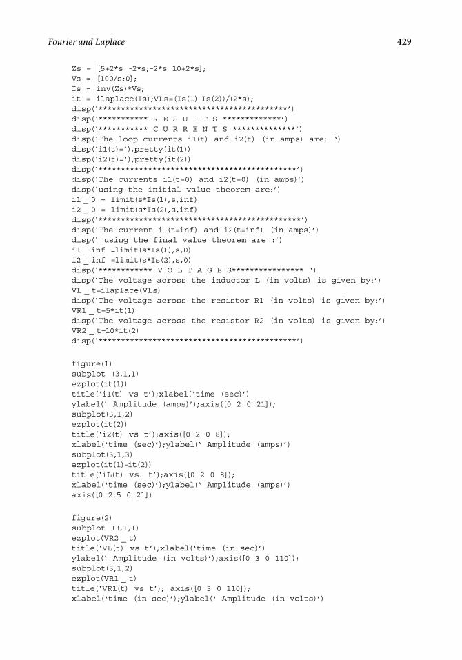
Fourier and Laplace 429
Zs = [5+2*s -2*s;-2*s 10+2*s];Vs = [100/s;0];Is = inv(Zs)*Vs;it = ilaplace(Is);VLs=(Is(1)-Is(2))/(2*s);disp(‘******************************************’)disp(‘*********** R E S U L T S *************’)disp(‘*********** C U R R E N T S **************’)disp(‘The loop currents i1(t) and i2(t) (in amps) are: ‘)disp(‘i1(t)=’),pretty(it(1))disp(‘i2(t)=’),pretty(it(2))disp(‘********************************************’)disp(‘The currents i1(t=0) and i2(t=0) (in amps)’)disp(‘using the initial value theorem are:’)i1 _ 0 = limit(s*Is(1),s,inf)i2 _ 0 = limit(s*Is(2),s,inf)disp(‘*********************************************’)disp(‘The current i1(t=inf) and i2(t=inf) (in amps)’)disp(‘ using the final value theorem are :’)i1 _ inf =limit(s*Is(1),s,0)i2 _ inf =limit(s*Is(2),s,0)disp(‘************ V O L T A G E S**************** ‘)disp(‘The voltage across the inductor L (in volts) is given by:’)VL _ t=ilaplace(VLs)disp(‘The voltage across the resistor R1 (in volts) is given by:’)VR1 _ t=5*it(1)disp(‘The voltage across the resistor R2 (in volts) is given by:’)VR2 _ t=10*it(2)disp(‘********************************************’)
figure(1)subplot (3,1,1)ezplot(it(1))title(‘i1(t) vs t’);xlabel(‘time (sec)’)ylabel(‘ Amplitude (amps)’);axis([0 2 0 21]);subplot(3,1,2)ezplot(it(2))title(‘i2(t) vs t’);axis([0 2 0 8]);xlabel(‘time (sec)’);ylabel(‘ Amplitude (amps)’)subplot(3,1,3)ezplot(it(1)-it(2))title(‘iL(t) vs. t’);axis([0 2 0 8]);xlabel(‘time (sec)’);ylabel(‘ Amplitude (amps)’)axis([0 2.5 0 21])
figure(2)subplot (3,1,1)ezplot(VR2 _ t)title(‘VL(t) vs t’);xlabel(‘time (in sec)’)ylabel(‘ Amplitude (in volts)’);axis([0 3 0 110]);subplot(3,1,2)ezplot(VR1 _ t)title(‘VR1(t) vs t’); axis([0 3 0 110]);xlabel(‘time (in sec)’);ylabel(‘ Amplitude (in volts)’)
CRC_47760_CH004.indd 429CRC_47760_CH004.indd 429 7/28/2008 12:26:18 PM7/28/2008 12:26:18 PM

430 Practical MATLAB® Applications for Engineers
subplot(3,1,3)ezplot(VR2 _ t)title(‘VR2(t) vs. t’);axis([0 3 0 110]);xlabel(‘time (in sec)’);ylabel(‘ Amplitude (in volts)’)
The script fi le loop_laplace_eqs is executed and the results are as follows (Figures 4.75 and 4.76):
>> loop _ laplace _ eqs
***************************************************** R E S U L T S ************************ C U R R E N T S **************The loop currents i1(t) and i2(t) (in amps) are: i1(t)= - 40/3 exp(- 5/3 t) + 20i2(t)= 20/3 exp(- 5/3 t)********************************************The currents i1(t=0) and i2(t=0) (in amps)using the initial value theorem are:i1 _ 0 = 20/3i2 _ 0 = 20/3*********************************************The current i1(t=inf) and i2(t=inf) (in amps) using the final value theorem are :i1 _ inf = 20 i2 _ inf = 0
************ V O L T A G E S**************** The voltage across the inductor L (in volts) is given by:
VL _ t = 6*exp(-5/3*t)+10*t-6
The voltage across the resistor R1 (in volts) is given by:
VR1 _ t = -200/3*exp(-5/3*t)+100
The voltage across the resistor R2 (in volts) is given by:
VR2 _ t = 200/3*exp(-5/3*t)
Note that at t = 0, the inductor acts as an open circuit, then i1(0) = i2(0) = 100 V/15 Ω =20/3 A; and at t = ∞, the inductor becomes a short circuit, then i1(∞) = 100 V/5 Ω = 20 A,and i2(∞) = 0 A. Values that completely agree with the results obtained using the MATLAB symbolic toolbox.
CRC_47760_CH004.indd 430CRC_47760_CH004.indd 430 7/28/2008 12:26:19 PM7/28/2008 12:26:19 PM

Fourier and Laplace 431
20
10
0
20
10
00 1 2 2.50.5 1.5
0 1 21.2 1.4 1.6 1.80.2 0.4 0.6 0.8
00
1 21.2 1.4 1.6 1.80.2 0.4 0.6 0.8
8
6
4
2
time (sec)
time (sec)
time (sec)
iL(t) versus t
i2(t) versus t
i1(t) versus t
Am
plitu
de (
amps
)A
mpl
itude
(am
ps)
Am
plitu
de (
amps
)
FIGURE 4.75Current plots of Example 4.18.
FIGURE 4.76Voltage plots of Example 4.18.
VR2(t) versus t
VR1(t) versus t
VL(t) versus t
Am
plitu
de (
in v
olts
)A
mpl
itude
(in
vol
ts)
Am
plitu
de (
in v
olts
)
100
50
0
100
50
0
100
50
0
0 1 2 3
time (in sec)
time (in sec)
time (in sec)
2.51.50.5
0 1 2 32.51.50.5
0 1 2 32.51.50.5
CRC_47760_CH004.indd 431CRC_47760_CH004.indd 431 7/28/2008 12:26:19 PM7/28/2008 12:26:19 PM

432 Practical MATLAB® Applications for Engineers
Example 4.19
The switch in the circuit diagram of Figure 4.77 closes at t = 0, where it remains for t > 0.The storing energy elements such as the (two) capacitors and the (two) inductors are
initially charged as indicated in Figure 4.77 (for t = 0).
1. Redraw the equivalent circuit in the s-domain 2. Obtain in the s-domain the loop equations 3. Obtain the matrix loop equation of part 2 4. Use MATLAB and obtain expressions for I1(s) and I2(s) 5. Obtain the system’s poles 6. Use MATLAB and verify the initial and fi nal value loop currents by applying the
initial and fi nal value theorems 7. Use MATLAB and obtain plots of I1(s) versus s and I2(s) versus s 8. Discuss the results
The MATLAB solution is given as follows by e script fi le IC_loop_diff_eqs.
ANALYTICAL Solution
Part 1 The time domain circuit shown in Figure 4.77 is transformed into the equivalent
s-domain circuit shown in Figure 4.78, where the initial conditions are converted into sources, and the assumed loop currents directions of I1(s) and I2(s) are indicated.
Part 2 The two loop equations of the circuit diagram of Figure 4.78 are
For loop #1:
502
35
2 231 2s s
ss
I ss
I s
( ) ( )
For loop #2:
39
4 159
23 3 7
52 1s s s s
I s ss
I
( ) 22( )s
v1(t ) = 50V
V2
sw closes at t = 0 L1 = 1 H L 2 = 3 HR1 = 2 Ω
R2 = 3 Ω
R 3 = 4 Ω
C1 = 0.5 F
C2 = 0.33 F
IL1(o) = 2 AIL2(0) = 3 A
+
VC1(0) = 3 V
−
+
VC2(0) = 4 V
−
(t ) = 5sin(3t ) V
+
−
FIGURE 4.77Circuit diagram of Example 4.19.
CRC_47760_CH004.indd 432CRC_47760_CH004.indd 432 7/28/2008 12:26:19 PM7/28/2008 12:26:19 PM

Fourier and Laplace 433
V1(s) = 50/s
V2(s) =
ZL1(s) = s
ZC1(s) = 2/s
R1(s) = 2
R 2 (s) = 3
R3 (s) = 4ZL2(s) = 3 s
ZC2(s) = 3/sI1(s)
I2(s)
2 V 9 V
3/s4/s
15s2+9
−−
++
FIGURE 4.78Equivalent s-domain circuit of Figure 4.77.
Part 3 The Matrix loop equation is given by
502
3
19
159
52 2
3
23 3 4
52
s s
s s
ss s
ss
s
I ss
I s
1
2
2( )
( )
MATLAB Solution% Script file: IC _ loop _ diff _ eqssyms s Zs Is Vs it yZs = [s+5+2/s -2/s-3;-2/s-3 3*s+7+5/s];Vs = [50/s+2-3/s;-1/s-9-15/(s^2+9)];Is = inv(Zs)*Vs;it = ilaplace(Is);disp(‘*********************************************************’)disp(‘************* Frequency domain Results ***************’)disp(‘*********************************************************’)disp(‘The loop currents I1(s) and I2(s) are: ‘)disp(‘I1(s)=’),pretty(Is(1))disp(‘I2(s)=’),pretty(Is(2))disp(‘***************************************************’)disp(‘The values of the currents (in amps) i1(0) and i2(0), and’) disp(‘i1(t=inf) and i2(t=inf) using the initial and final value theorems’)disp(‘are verified below:’)i1 _ 0 = limit(s*Is(1),s,inf)i2 _ 0 = limit(s*Is(2),s,inf)i1 _ inf = limit(s*Is(1),s,0)i2 _ inf = limit(s*Is(2),s,0)disp(‘*********************************************************’)den = [3 22 37 27 6];disp(‘The system poles are:’)rr = roots(den);abs(rr)disp(‘***************************************************’)
CRC_47760_CH004.indd 433CRC_47760_CH004.indd 433 7/28/2008 12:26:19 PM7/28/2008 12:26:19 PM

434 Practical MATLAB® Applications for Engineers
figure(1)ezplot(Is(1))title(‘I1(s) vs s’)xlabel(‘ complex frequency s ‘)ylabel(‘I1(s) ‘)ylabel(Amplitude’)figure(2)ezplot(Is(2))title(‘I2(s) vs s’);xlabel(‘complex frequency s’);ylabel(‘Amplitude’)disp(‘***************************************************’)disp(‘******************* RESULTS **********************’)disp(‘***************************************************’)disp(‘The loop currents i1(t) and i2(t) (in amps) are: ‘)disp(‘i1(t)=’),pretty(it(1))disp(‘i2(t)=’),pretty(it(2))disp(‘****************************************************’)
The script fi le IC_loop_diff_eqs is executed and the results are as follows (Figures 4.79 and 4.80):
>> IC _ loop _ diff _ eqs
****************************************************************** RESULTS **************************************************************************
The loop currents I1(s) and I2(s) are:
/ 15 \ 2 / 47 \ (2 + 3 s) s |- 1/s - 9 - ------ | (3 s + 7 s + 5) s |---- + 2 | | 2 | \ s / \ s + 9 / I1(s) = ------------------------------- + -------------------------------- 4 3 4 3 2 3 s + 22 s + 37 s + 27 s + 6 3 s + 22 s + 37 s + 27 s + 6
2 / 15 \ / 47 \ (s + 5 s + 2) s |- 1/s - 9 - ------ | (2 + 3 s) s |---- + 2 | | 2 | \ s / \ s + 9 / I2(s) = ------------------------------- + ---------------------------------- 4 3 2 4 3 2 3 s + 22 s + 37 s + 27 s + 6 3 s + 22 s + 37 s + 27 s + 6
***************************************************The values of the currents (in amps) i1(0) and i2(0), and i1(t=inf) and i2(t=inf) using the initial and final value theorems are verified below:
i1 _ 0 = 2i2 _ 0 = -3i1 _ inf = 0i2 _ inf = 0
CRC_47760_CH004.indd 434CRC_47760_CH004.indd 434 7/28/2008 12:26:19 PM7/28/2008 12:26:19 PM

Fourier and Laplace 435
FIGURE 4.79Plot of I1(s) of Example 4.19.
20
15
10
5
0
0 2 4 6
−5
−10
−15
−20−6 −4 −2
complex frequency s
Am
plitu
de
I1 (s) versus s
FIGURE 4.80Plot of I2(s) of Example 4.19.
20
15
10
5
0
0 2 4 6
−5
−10
−6 −4 −2
complex frequency s
Am
plitu
de
I2 (s) versus s
CRC_47760_CH004.indd 435CRC_47760_CH004.indd 435 7/28/2008 12:26:20 PM7/28/2008 12:26:20 PM

436 Practical MATLAB® Applications for Engineers
***************************************************The system poles are:ans = 5.3196 1.0051 1.0051 0.3721
Note that all the poles of I1(s) and I2(s) are in the left half of the s-plane, then the initial and fi nal value theorems can be used. Note also that the initial currents are verifi ed, and the fi nal currents are zero since the two capacitors for t = ∞ act as an open circuit.
Example 4.20
The switch in the circuit diagram of Figure 4.81 closes at t = 0, where it remains for t > 0. All the storing elements are initially charged as indicated in Figure 4.81, at t = 0.
1. Redraw the equivalent circuit in the s-domain 2. Write the s-domain node equations 3. Write the matrix node equation 4. Use MATLAB and obtain expressions for V1(s) and V2(s) 5. Use MATLAB and obtain plots of V1(s) versus s and V2(s) versus s 6. Use MATLAB to evaluate and verify the initial and fi nal voltage for each node by
applying the initial and fi nal value theorems
The MATLAB solution is given as follows by the script fi le nodal _eqs:
ANALYTICAL Solution
Part 1
The time domain circuit diagram of Figure 4.80 is redrawn in the s-domain shown in Figure 4.82, indicating the two nodal voltages V1(s) and V2(s) and the circuit ini-tial conditions transformed into sources.
Part 2
The two nodal equations are
For node # 1V
s ss
sV s
sV: ( )
52
3 13
14 2
13
13
141
22( )s
For node # :2V
s ss
s sI s
s s3 2 8
913
14
14
19
13
152 1
( )
V s2( )
Part 3 The node matrix equation in the s domain is given by
22
3 89
13
712 2
13
14
13
14
1336
8152
s
ss
s
ss
s
s
ss
V s
V s
1
2
( )
( )
MATLAB Solution% Script file: nodal _ eqssyms s Ys Is Vs it yYs = [7/12+s/2+1/(3*s) -(1/4+1/(3*s));-(1/4+1/(3*s)) 13/36+8/(15*s)];
CRC_47760_CH004.indd 436CRC_47760_CH004.indd 436 7/28/2008 12:26:20 PM7/28/2008 12:26:20 PM

Fourier and Laplace 437
Is = [2/s+2;8*s/(s^2-9)+1/s];Vs =inv(Ys)*Is;disp(‘*********************************’)disp(‘********* RESULTS ************’)disp(‘*********************************’)disp(‘The node voltages V1(s) and V2(s) are: ‘)disp(‘V1(s)=’),pretty(Vs(1))disp(‘V2(s)=’),pretty(Vs(2))disp(‘************************************’)disp(‘The initial value voltages V1(t=0) and V2(t=0) (in volts)’)disp(‘using the initial value theorem are verified returning:’)V1 _ 0 = limit(s*Vs(1),s,inf)V2 _ 0 = limit(s*Vs(2),s,inf)disp(‘************************************’)disp(‘The final value voltages V1(t=inf) and V2(t=inf) (in volts)’)
i1(t ) = 5 A
i2(t ) = 8 cos(3t ) A
R1 = 3 Ω
R2 = 4 Ω
R3 = 9 Ω
C1 = 0.5 F
L1 = 3 h
sw closes at t = 0
L2 = 5 H
v1(t )
v1(t )
v2(t )
+
VC 1(0) = 4 V
−
IL1(0) = 3 A
IL 2(0) = 2 A
FIGURE 4.81Circuit diagram of Example 12.20.
I1(s) = 5/s
I2(s) =
R1 = 3
ZC1(S ) = 2/s
R 2 = 4
ZL1(s) = 3 s
sw Closes at t = 0
ZL2(S ) = 5s R3 = 9
V1(s) V2(s)
2 A
3/s
2/ss2+98s
FIGURE 4.82Equivalent s-domain circuit of Figure 4.81.
CRC_47760_CH004.indd 437CRC_47760_CH004.indd 437 7/28/2008 12:26:20 PM7/28/2008 12:26:20 PM

438 Practical MATLAB® Applications for Engineers
disp(‘using the final value theorem are verified returning: ‘)V1 _ inf =limit(s*Vs(1),s,0)V2 _ inf =limit(s*Vs(2),s,0)disp(‘************************************’)figure(1)ezplot(Vs(1))title(‘V1(s) vs s’)xlabel(‘ complex frequency s ‘);ylabel(‘V1(s) ‘)figure(2)ezplot(Vs(2))title(‘V2(s) vs s’);xlabel(‘complex frequency s’);ylabel(‘V2(s) ‘)
The script fi le nodal _eqs is executed and the results are as follows (Figures 4.83 and 4.84):
>> nodal _ eqs****************************************** RESULTS *********************************************The node voltages V1(s) and V2(s) are:
/ s \ (3 s + 4) s |8 ------ + 1/s| | 2 | (65 s + 96) s (2/s + 2) \ s + 9 / V1(s) = 6 ---------------------------- + 90 ---------------------------- 2 3 2 3 448 s + 286 s + 195 s + 72 448 s + 286 s + 195 s + 72
2 / s \ (7 s + 6 s + 4) s |8 ------ + 1/s| | 2 | (3 s + 4) s (2/s + 2) \ s + 9 / V2(s) = 90 ---------------------------- + 90 ----------------------------------- 2 3 2 3 448 s + 286 s + 195 s + 72 448 s + 286 s + 195 s + 72
*****************************************************The initial value voltages V1(t=0) and V2(t=0) (in volts)using the initial value theorem are verified returning:
V1 _ 0 = 4V2 _ 0 = 360/13
*****************************************************The final value voltages V1(t=inf) and V2(t=inf) (in volts)using the final value theorem are verified returning:
V1 _ inf = 0V2 _ inf = 0
******************************************************
CRC_47760_CH004.indd 438CRC_47760_CH004.indd 438 7/28/2008 12:26:21 PM7/28/2008 12:26:21 PM

Fourier and Laplace 439
−4
−4
−2
−6
−2 0 2 4 6complex frequency s
14
12
10
8
6
4
2
0
V1
(s)
V1 (s) versus s
FIGURE 4.83Plot of V1(s) of Example 4.20.
−6
−20
−10
−4 −2 0
0
10
20
30
complex frequency s2 4 6
V2(
s)
V2(s) versus s
FIGURE 4.84Plot of V2(s) of Example 4.20.
Example 4.21
The switch in the circuit diagram shown in Figure 4.85 closes at t = 0, and the network is unenergized before the switch is closed, with i1(t = 0) = i2(t = 0) = 0.A.
1. Write the set of loop equations in the time domain (the assumed directions of i1(t) and i2(t) are indicated in Figure 4.85)
2. Transform the equations of part 1 into the s-domain 3. Obtain the matrix loop equations in the s-domain and indicate the impedance
matrix z(s) and voltage vector v(s)
CRC_47760_CH004.indd 439CRC_47760_CH004.indd 439 7/28/2008 12:26:21 PM7/28/2008 12:26:21 PM

440 Practical MATLAB® Applications for Engineers
4. Use MATLAB and obtain expressions for I1(s) and I2(s) 5. Use MATLAB to evaluate the initial- and fi nal value of each loop current by apply-
ing the initial and fi nal value theorems 6. Use MATLAB to obtain solutions for i1(t) and i2(t), for t ≥ 0 7. Use MATLAB to obtain plots of i1(t) versus t and i2(t) versus t, for t ≥ 0 8. Discuss the results obtained
The MATLAB solution is given as follows by the script fi le loop_diffeqs:
ANALYTICAL Solution
Part 1
The loop equations in the time domain for t ≥ 0 are
100 20 10
0 10 20
11 2
1 22
u tdi t
dti t i t
i t i tdi t
d
( )( )
( ) ( )
( ) ( )( )
tt
Part 2
The loop equations in the frequency domain are
10020 10
0 10 20
1 2
1 2
ss I s I s
I s s I s
( ) ( ) ( )
( ) ( ) ( )
Part 3
The matrix loop equation of the network in the frequency domain is given by
1000
20 1010 20
1
2
s s
s
I s
I s
( )( )
V1 = 100 V
R1 = 10 Ω L1 = 1 H
i1(t )i2(t )
sw closes at t = 0
L2 = 1 H
R 2 = 10 Ω R3 = 10 Ω
FIGURE 4.85Circuit diagram of Example 4.21.
CRC_47760_CH004.indd 440CRC_47760_CH004.indd 440 7/28/2008 12:26:22 PM7/28/2008 12:26:22 PM

Fourier and Laplace 441
where Z s
s
s( )
20 1010 20
and
V ss
( ) 100
0
MATLAB Solution% Script file: loop _ diffeqssyms s Zs Is Vs Zs = [s+20 -10;-10 s+20];Vs = [100/s;0];Is = inv(Zs)*Vs;disp(‘*********************************************’)disp(‘********* Matlab Symbolic Results **********’)disp(‘*********************************************’)disp(‘The loop currents I1(s) and I2(s) are: ‘)disp(‘I1(s)=’),pretty(Is(1))disp(‘I2(s)=’),pretty(Is(2))disp(‘*********************************************’)i1 _ t = ilaplace(Is(1));i2 _ t = ilaplace(Is(2));disp(‘The loop currents i1(t) and i2(t)(in amp) are: ’)disp(‘i1(t)=’),simplify(i1 _ t) disp(‘i2(t)=’),simplify(i2 _ t)disp(‘**********************************************’)disp(‘The initial currents:i1(t=0) and i2(t=0)(in amps)’)disp(‘using the initial value theorem are evaluated below’)I1 _ 0 = limit(s*Is(1),s,inf)I2 _ 0 = limit(s*Is(2),s,inf)disp(‘**********************************************’)disp(‘The final currents:i1(t=inf) and i2(t=inf)(in amps)’)disp(‘using the initial value theorem are:’)I1 _ inf = limit(s*Is(1),s,0)I2 _ inf = limit(s*Is(2),s,0)disp(‘**********************************************’)
figure(1)subplot(1,2,1)ezplot(i1 _ t);axis([0 .5 0 7])title(‘i1(t) vs t’),xlabel(‘time (sec)’)ylabel(‘i1(t) in amp’)subplot(1,2,2)ezplot(i2 _ t);axis([0 .5 0 3.5])title(‘i2(t) vs t’)xlabel(‘ time (sec) ‘)ylabel(‘i2(t) in amp ‘)
The script fi le loop_diffeqs is executed and the results are as follows:
CRC_47760_CH004.indd 441CRC_47760_CH004.indd 441 7/28/2008 12:26:22 PM7/28/2008 12:26:22 PM

442 Practical MATLAB® Applications for Engineers
>> loop _ diffeqs
****************************************************** Matlab Symbolic Results *******************************************************The loop currents I1(s) and I2(s) are:
s + 20 I1(s) = 100 ------------------- 2 (s + 40 s + 300) s
1000 I2(s) = ------------------- 2 (s + 40 s + 300) s*********************************************The loop currents i1(t) and i2(t) (in amp) are: i1(t) = -5/3*exp(-30*t)-5*exp(-10*t)+20/3
i2(t) = 10/3-5*exp(-10*t)+5/3*exp(-30*t)**********************************************The initial currents: i1(t=0) and i2(t=0) (in amps)using the initial value theorem are evaluated below: I1 _ 0 = 0I2 _ 0 = 0**********************************************The final currents: i1(t=inf) and i2(t=inf) (in amps)using the final value theorem are: I1 _ inf = 20/3I2 _ inf = 10/3**********************************************
Note that at t = ∞, the two inductors become shorts, then i1(∞) = 100 V/15 Ω = 20/3 A, and i2(∞) = i1(∞)/2 = 10/3 A.
Observe that the analytical solutions agree completely with the MATLAB results (see Figure 4.86).
00
1
2
3
4
5
6
7
0.1 0.2 0.3 0.4time (sec)
0 0.1 0.2 0.3 0.4time (sec)
i 1(t)
in a
mps
i 2(t)
in a
mps
3.5
3
2
1
0
0.5
1.5
2.5
i1 (t) versus t i2 (t) versus t
FIGURE 4.86Current plots of i1(t) and i2(t) of Example 4.21.
CRC_47760_CH004.indd 442CRC_47760_CH004.indd 442 7/28/2008 12:26:22 PM7/28/2008 12:26:22 PM

Fourier and Laplace 443
Example 4.22
Modulated signals are often encountered in telecommunications and consist of mixing (multiplying) two analog signals referred to as the message signal m(t), consisting of low frequencies; and the carrier signal c(t), consisting of a high-frequency sinusoidal.
Let the modulating and carrier signals be given by m(t) = 3 cos(5t) and c(t) = cos(50t), respectively.
Create the MATLAB script fi le telecom_signals that returns
1. Expressions of a. C(w) = ℑ[c(t)] b. M(w) = ℑ[m(t)] c. M(w) + C(w) = ℑ[m(t)] + ℑ[c(t)] d. AM_DSB_SC(w) = ℑ[m(t) c(t)] = 1/2π(ℑ[M(w) ⊗ C(w)]* e. AM_DSB_WC(w) = ℑ[(m(t) + 5) c(t)] f. FM(w) = ℑ[fm(t)] = ℑ[cos(50 t + m(t))]
2. The following time and frequency plots: a. m(t) versus t ↔ M(w) versus w b. c(t) versus t ↔ C(w) versus w c. [m(t) + c(t)] versus t ↔ [M(w) + C(w)] versus w d. m(t) c(t) versus t ↔ ℑ [m(t) c(t)] e. [m(t)+5 c(t)] versus t ↔ ℑ [(m(t) + 5) c(t)] versus w f. cos[50 t + m(t)] versus t ↔ ℑcos[(50t) + m(t)] versus w
ANALYTICAL Solution
An AM signal is a signal in which (m(t) cos(w0t)), the amplitude of the carrier, is modu-lated by the message wave m(t); hence the information content of m(t) is carried by the amplitude variations of the carrier.
If the angle of the carrier varies in some manner with respect to the modulation signal m(t), then the modulation technique is referred to as angle modulation given by the following equation:
cos(w0t) + f(m(t)) The following two methods are used in the generation of angle modulation:
1. PM 2. FM
PM and FM are defi ned by the following equations:
1. pm(t) = A cos[w0t + kam(t)] 2. fm(t) = A cos[w0t + kb ∫m(t) dt(m(t)]
where A, ka, and kb are constants.It is easy to appreciate that although PM and FM are different forms of angle modulation,
they are essentially very similar, specially if the message signal is a sinusoidal. Therefore, it is unnecessary to discuss the two modulation methods, and one is suffi cient to illustrate the process. For simplicity, fm(t) will be referred as an angular-modulated signal.
AM spectrum expressions can directly be obtained by using the MATLAB function fourier.
* AM stands for amplitude modulation, DSB for double side band, SC for suppress carrier, WC for with carrier, and FM for frequency modulation.
CRC_47760_CH004.indd 443CRC_47760_CH004.indd 443 7/28/2008 12:26:22 PM7/28/2008 12:26:22 PM

444 Practical MATLAB® Applications for Engineers
The FM spectrums can be obtained by the expansion of the time function in terms of the Bessel functions, illustrated as follows:
A w t km t A j k w t j k w w t w wm[cos( ( ))] ( )cos ( )[cos( ) cos(0 0 0 1 0 0 mm
m m
m
t
j k w w t w w t
j k w w t
) ]
( )[cos( ) cos( ) ]
( )[cos( )
2 0 0
3 0
2 2
3
ccos( ) ]
( )[cos( ) cos( ) ]
( )[cos
w w t
j k w w t w w t
j k
m
m m
n
0
4 0 0
3
4 4
…
(( ) cos( ) ]w nw t w nw tm m0 0 where wm is the highest frequency of m(t), and jn(k) denotes the Bessel function of the fi rst kind and nth order (referred to the command besselj in MATLAB).
In general, the jn(k)s are negligible for n > k, if k > 1.
MATLAB Solution% Script file : telecom _ signalssyms t w m _ t c _ t AM FM fmm _ t = 3*cos(5*t);c _ t = cos(50*t);disp (‘*********************************************************************’)disp (‘************************* R E S U L T S *******************************’)disp (‘The spectrum of the communication signals are:’)disp(‘*********************************************************************’)Cw _ spectrum _ of _ carrier=fourier(c _ t)disp (‘*********************************************************************’)Mw _ spectrum _ of _ message = fourier(m _ t)disp(‘**********************************************************************’)MCw _ spectrum _ carry _ plus _ message = fourier(m _ t+c _ t)disp(‘**********************************************************************’)AM _ DSB _ SC _ spectrum _ =fourier(c _ t*m _ t)disp(‘**********************************************************************’)AM _ DSB _ WC _ spectrum _ =fourier(c _ t*(m _ t+5))disp(‘**********************************************************************’)fm=besselj(3,0)*cos(50*t)+besselj(3,1)*(cos((50+5)*t)-cos((50-5)*t));fm=fm+besselj(3,2)*(cos((50+5*2)*t)+cos((50-5*2)*t))+besselj(3,3)*(cos ((50+5*3)*t)- cos((50-5*3)*t));fm= fm+besselj(3,4)*(cos((50+5*4)*t)+cos((50-5*4)*t));fm=fm+besselj(3,5)*(cos((50+5*5)*t)-cos((50-5*5)*t));spectrum _ fm=fourier(fm);FM _ spectrum=vpa(spectrum _ fm,3)disp(‘**********************************************************************’)
figure(1)subplot(3,2,1);fplot(‘3*cos(5*t)’,[0 3 -6 6]);title(‘TIME DOMAIN’);ylabel(‘message(t)’);subplot(3,2,2)w _ mes=[-5 5];mag _ mes=[3*pi 3*pi];stem(w _ mes,mag _ mes)title(‘FREQUENCY DOMAIN’)
CRC_47760_CH004.indd 444CRC_47760_CH004.indd 444 7/28/2008 12:26:23 PM7/28/2008 12:26:23 PM
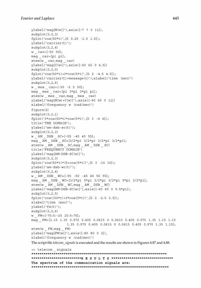
Fourier and Laplace 445
ylabel(‘mag[M(w)]’),axis([-7 7 0 11]),subplot(3,2,3)fplot(‘cos(50*t)’,[0 0.25 -1.5 1.5]);ylabel(‘carrier(t)’);subplot(3,2,4)w _ car=[-50 50];mag _ car=[pi pi];stem(w _ car,mag _ car)ylabel(‘mag[C(w)]’),axis([-60 60 0 4.5])subplot(3,2,5)fplot(‘cos(50*t)+3*cos(5*t)’,[0 2 -4.5 4.5]);ylabel(‘carrier(t)+message(t)’);xlabel(‘time (sec)’)subplot(3,2,6)w _ mes _ car=[-50 -5 5 50];mag _ mes _ car=[pi 3*pi 3*pi pi];stem(w _ mes _ car,mag _ mes _ car)ylabel(‘mag[M(w)+C(w)]’),axis([-60 60 0 11])xlabel(‘frequency w (rad/sec)’)
figure(2)subplot(3,2,1)fplot(‘3*cos(50*t)*cos(5*t)’,[0 3 -6 6]);title(‘TME DOMAIN’);ylabel(‘am-dsb-sc(t)’);subplot(3,2,2)w _ AM _ DSB _ SC=[-55 -45 45 55];mag _ AM _ DSB _ SC=[3/2*pi 3/2*pi 3/2*pi 3/2*pi];stem(w _ AM _ DSB _ SC,mag _ AM _ DSB _ SC)title(‘FREQUENCY DOMAIN’)ylabel(‘mag[AM-DSB-SC(w)]’);subplot(3,2,3)fplot(‘cos(50*t)*(5+cos(5*t))’,[0 3 -10 10]);ylabel(‘am-dsb-wc(t)’);subplot(3,2,4)w _ AM _ DSB _ WC=[-55 -50 -45 45 50 55];mag _ AM _ DSB _ WC=[3/2*pi 5*pi 3/2*pi 3/2*pi 5*pi 3/2*pi];stem(w _ AM _ DSB _ WC,mag _ AM _ DSB _ WC)ylabel(‘mag[AM-DSB-SC(w)]’),axis([-60 60 0 5.5*pi]),subplot(3,2,5)fplot(‘cos((50*t)+3*cos(5*t))’,[0 2 -2.5 2.5]);xlabel(‘time (sec)’);ylabel(‘fm(t)’);subplot(3,2,6)w _ FM=[-75:5:-25 25:5:75];mag _ FM=[1.15 1.35 0.970 0.405 0.0615 0 0.0615 0.405 0.970 1.35 1.15 1.15 1.35 0.970 0.405 0.0615 0 0.0615 0.405 0.970 1.35 1.15];stem(w _ FM,mag _ FM)ylabel(‘mag[FM(w)]’),axis([-80 80 0 2]),xlabel(‘frequency w (rad/sec)’)
The script fi le telecom_signals is executed and the results are shown in Figures 4.87 and 4.88.
>> telecom _ signals*********************************************************************************************R E S U L T S *******************************The spectrum of the communication signals are:*********************************************************************
CRC_47760_CH004.indd 445CRC_47760_CH004.indd 445 7/28/2008 12:26:23 PM7/28/2008 12:26:23 PM

446 Practical MATLAB® Applications for Engineers
Cw _ spectrum _ of _ carrier = pi*Dirac(w-50)+pi*Dirac(w+50)*********************************************************************
Mw _ spectrum _ of _ message = 3*pi*Dirac(w-5)+3*pi*Dirac(w+5)*********************************************************************MCw _ spectrum _ carry _ plus _ message = 3*pi*Dirac(w-5)+3*pi*Dirac(w+5)+pi*Dirac(w-50)+pi*Dirac(w+50)**********************************************************************AM _ DSB _ SC _ spectrum _ = 3/2*pi*Dirac(w-55)+3/2*pi*Dirac(w- 45)+3/2*pi*Dirac(w+45)+3/ 2*pi*Dirac(w+55)***********************************************************************AM _ DSB _ WC _ spectrum _ = 3/2*pi*Dirac(w-55)+3/2*pi*Dirac(w-45)+5*pi*Dirac(w-0)+3/2*pi*Dirac(w+45)+3/2*pi*Dirac(w+55)+5*pi*Dirac(w+50)
***********************************************************************FM _ spectrum = .615e-1*Dirac(w-55.)+.615e-1*Dirac(w+55.)-.615e-1*Dirac(w-45.)-.615e-1*Dirac(w+45.)+.405*Dirac(w-60.)+.405*Dirac(w+60.)+.405*Dirac(w-40.)+.405*Dirac(w+40.)+.970*Dirac(w-65.)+.970*Dirac(w+65.)-.970*Dirac(w-35.)-.970*Dirac(w+35.)+1.35*Dirac(w-70.)+ 1.35*Dirac(w+70.)+ 1.35*Dirac(w-30.)+1.35*Dirac(w+30.)+1.15*Dirac(w-75.)+1.15*Dirac(w+75.)- 1.15*Dirac(w-25.)-1.15*Dirac(w+25.)*************************************************************************
5
5
50
0
0
10
0
0.05 0.15
1.5 50
0
0
0 00
5
10
0.5
4
2
−2
−50
500
0−50
−4
0
1
0.1 0.2
1
1 2
2 3−5
−1
−5
time (sec)
4
2
mes
sage
(t)
carr
ier(
t)ca
rrie
r(t)
+m
essa
ge(t
)
mag
[M(w
)]m
ag[C
(w)]
mag
[M(w
)]+
C(w
)]
frequency w (rad/sec)
TIME DOMAIN FREQUENCY DOMAIN
FIGURE 4.87Time and frequency domain of parts a, b, and c of Example 4.22.
CRC_47760_CH004.indd 446CRC_47760_CH004.indd 446 7/28/2008 12:26:23 PM7/28/2008 12:26:23 PM

Fourier and Laplace 447
FIGURE 4.88Time and frequency domain of parts d, e, and f of Example 4.22.
0
0
5
−51 2 3
0 1 2 3
0
0
0
2
−2
−10
10
0.5 21 1.5time (sec)
fm(t
)am
-dsb
-wc(
t)am
-dsb
-sc(
t)
−100 −50
−50
0
0
50
10
15
50
−50 0 50
1000
0
0
1
2
2
4
5
6
frequency w (rad/sec)
mag
[FM
(w)]
mag
[AM
-DS
B-S
C(w
)]m
ag[A
M-D
SB
-SC
(w)]TIME DOMAIN FREQUENCY DOMAIN
4.5 Application Problems
P.4.1 Given the functions shown in Figure 4.89, draw the even and odd parts for each func-tion by hand, and determine the trigonometric FS of each part using MATLAB.
P.4.2 Write a function fi le that returns the energy of a given arbitrary function f(t). Test your fi le for each of the functions shown in Figure 4.89.
P.4.3 Let the FS for the function f1(t) be given by
f t
nnt
n1 )( )
12
1 1
1
∑ sin(2
Evaluate the energy of f1(t) in the frequency and the time domain.P.4.4 Using the trigonometric FS given in P.4.3, write a MATLAB program that returns
the following plots:a. f1(t) vs. t
b. The FS approximation of f1(t) using the fi rst fi ve terms versus t
c. Repeat part b for the fi rst 15 terms versus t
d. F1(w) versus w (magnitude and phase)e. Power of f1(t) versus t
CRC_47760_CH004.indd 447CRC_47760_CH004.indd 447 7/28/2008 12:26:24 PM7/28/2008 12:26:24 PM

448 Practical MATLAB® Applications for Engineers
tt
t t
−2 0 1 2
−1
−1+1
1
f 7(t )
f 4(t )
f 6(t )
f 5(t )
f 3(t )f 2(t )f 1(t )
2
0 1
1
0 2 −2 0 2
tt
t1
−1 −10 3
3
0 2 3
3
2
1
1.5
FIGURE 4.89Plots of P.4.1.
P.4.5 Let
f t
nnt
n2
1
12
1 12( ) sin( )
∑
Sketch by handa. f2(t) versus t
b. [f3(t) = 1 − f2(t)] versus t
c. mag[F3(w)] versus w
d. phase[F3(w)] versus w
P.4.6 Repeat P.4.5 using MATLAB.P.4.7 The script fi le drill returns the FS expansion of the function f(t), as shown in the
following, as well as its fi rst four partial FS approximations shown in Figure 4.90.
% Script file: drillw1=1; w3 =3; w5 =5; w7=7;k1= 4/pi;k3 = 4/(pi*3);k5 = 4/(pi*5);k7= 4/(pi*7);k = 0:pi/30:2*pi;x1 =k1*sin(w1*k);x3 = k3*sin(w3*k);
CRC_47760_CH004.indd 448CRC_47760_CH004.indd 448 7/28/2008 12:26:24 PM7/28/2008 12:26:24 PM

Fourier and Laplace 449
x5 = k5*sin(w5*k);x7 = k7*sin(w7*k);subplot(2,2,1);plot(k,x1)subplot(2,2,2);plot(k,x1+x3)subplot(2,2,3);plot(k,x1+x3+x5)subplot(2,2,4)plot (k,x1+x3+x5+x7) 11
Obtain the following: a. An expression of f(t)b. The fundamental frequency w0 and the period Tc. Properly label the axisd. Estimate the values of the Fourier coeffi cients F0 and F1
e. Estimate the 9th and 10th harmonicf. A neat fl ow chart of the programg. Estimate the discontinuity and the magnitude of f(t) at the discontinuities (Gibbs)
P.4.8 Let the FS of the functions f1(t) and f2(t) be given by
f t
nnt
n
n1
1
1
1( )
( )sin
∑ ( )
and
f t
nnt
n
n2
32
1
13
41
( )
( )
cos
∑ ( )
Determine or obtaina. The fundamental frequency, w0, for each of the given functionsb. The plots of f1(t) versus t and f2(t) versus t
c. The plots of F1(w) versus w and F2(w) versus w
0 2 4 6 8−2
−1
0
1
2
0 2 4 6 8−2
−1
0
1
2
0 2 4 6 8−2
−1
0
1
2
0 2 4 6 8−2
−1
0
1
2
FIGURE 4.90Plots of P.4.7.
CRC_47760_CH004.indd 449CRC_47760_CH004.indd 449 7/28/2008 12:26:24 PM7/28/2008 12:26:24 PM

450 Practical MATLAB® Applications for Engineers
d. The bandwidth of f1(t) and f2(t)e. The bandwidth of [f1(t) + f2(t)]
P.4.9 Evaluate the following FTs by hand, using Table 4.1:a. u(t)b. 3 + 2u(t)c. δ(t)d. δ(t − 2)e. 3δ(t − 4) + 6δ(t + 5)f. cos(15t)g. sin(2t)h. cos(15t) sin(2t)
P.4.10 Repeat P.4.9 by using the MATLAB symbolic toolbox.P.4.11 Using Table 4.1, determine by hand the following IFTs:
a. (Sin(w/ 2))/(w/ 2)b. δ(w)c. cos(3w)d. 2/(jw + 2)e. 3/(jw + 2)2
f. −1/w2
P.4.12 Repeat P.4.11 by using the MATLAB symbolic toolbox.P.4.13 Obtain using MATLAB expressions and plots (magnitude and phase) of
a. F1(w) = jw ______
2 + w2
b. F2(w) = 1 _______________ (1 + jw)(2 − jw)
P.4.14 Determine f1(t) and f2(t) for the following frequency functions:
a. F1(w) = j/(2 − w + jw)
b. F2(w) = 1 _______________ (1 + w2)(2 − jw)
P.4.15 Let
f t te u t F w
jwt( ) ( ) ( )
( )
2
2
12
↔
Obtain plots ofa. f(t) versus tb. mag[F(w)] versus wc. phase[F(w)] versus wd. [power of f(t)] versus w
P.4.16 Given the system shown in Figure 4.91, use MATLAB to obtain the following plots:a. x(t) versus tb. X(w) versus wc. Y(w) versus wd. y(t) versus t
CRC_47760_CH004.indd 450CRC_47760_CH004.indd 450 7/28/2008 12:26:24 PM7/28/2008 12:26:24 PM

Fourier and Laplace 451
h(t ) = x (t )
−1.5 0 1.5 t
input x(t )
output y (t )
x (t )1
FIGURE 4.91Block box system diagram of P.4.16.
R1 = 1 ΩR2 = 1 Ω
C = 2 F
Vi(w) V0(w)
FIGURE 4.92Circuit diagram of P.4.17.
P.4.17 Verify that the transfer function of the circuit diagram of Figure 4.92 is given by
H w
V wV w
jwjwi
( )( )( )
( / )( / )
0 1
21 21 4
a. Obtain plots of mag[H(w)] versus w and angle[H(w)] versus w
b. Estimate the circuit bandwidthc. Estimate the regions of nondistortion
P.4.18 Repeat problem P.4.17 for the RC network shown in Figure 4.93, where
H w
V wV w
jw jwjw jwi
( )( )( )
( . )( . )( ) . .
0
2
0 5 0 51 5 0 25
P.4.19 Verify that the transfer function of the RC network shown in Figure 4.94 is given by
H w
V wV w
jwjwi
( )( )( )
0 2 1
2 2
Estimate its bandwidth and the regions of nondistortion.P.4.20 Assuming that the input x(t) = cos(t) for the system diagram shown in Figure 4.91,
create a MATLAB script fi le that returns the following plots:a. x(t) versus t
b. X(w) versus w
c. h(t) versus t
d. mag[H(w)] versus w
CRC_47760_CH004.indd 451CRC_47760_CH004.indd 451 7/28/2008 12:26:24 PM7/28/2008 12:26:24 PM

452 Practical MATLAB® Applications for Engineers
e. angle[H(w)] versus w
f. mag[Y(w)] versus w
g. angle[Y(w)] versus w
h. y(t) versus t
P.4.21 Repeat P.4.20 for the cases where x(t) = u(t) + u(t − 1) − 2u(t − 2) and h(t) = 5t.
P.4.22 Evaluate the following LTs by hand, using Table 4.2:a. u(t) i. e−2tcos(10t) u(t)
b. 3 + 2u(t) j. sinh(10t) u(t)
c. δ(t) k. cosh(10t − π/4) u(t)
d. δ(t − 2) l. 2e−3t + 5 cos(3t) u(t)
e. 3δ(t − 4) + 6δ(t + 5) m. e−3tsin(10t + π/3) u(t)
f. cos(15t) u(t) n. 3e−2tu(−t)
g. sin(2t) u(t) o. cos(10t) cos(150t)
h. 5e−2t u(t) p. cos(10t)sin(150t)
P.4.23 Repeat P.4.22 using the MATLAB symbolic toolbox.P.4.24 Using Table 4.2, determine by hand the following ILTs:
a. sin(w/ 2)/(w/ 2)b. δ(w)
R = 1 Ω
R = 1 Ω
C = 2 F
C = 2 F
Vi(w) V0(w)
FIGURE 4.93Circuit diagram of P.4.18.
R = 1 Ω
R = 1 ΩC = 2 FVi(w) V0(w)
FIGURE 4.94Circuit diagram of P.4.19.
CRC_47760_CH004.indd 452CRC_47760_CH004.indd 452 7/28/2008 12:26:25 PM7/28/2008 12:26:25 PM

Fourier and Laplace 453
c. cos(3w)d. 2/(jw + 2)e. 3/(jw + 2)2
f. −1/w2
P.4.25 Using the MATLAB symbolic toolbox, repeat P.4.24.P.4.26 Obtain the following ILTs using Table 4.2, and indicate the Laplace properties used
in the process:a. (s + 3)/(s2 + 4s + 5)b. δ(s)c. cos(3s)d. (2s2 + 4s + 4)/(s2 + 3s + 2)e. s + 3/(s + 2)2
f. −1/s2
P.4.27 Verify that f(t) and F(s) given as follows constitute a LT pair
f t e t t e F s
se
s st t
s( ) sin( ) ( )
( )
3 4 4 3
32 16
23
2 2 33
2 3
↔
P.4.28 Find the partial fraction expansion of each of the following functions:a. 2s/(s2 + 5s + 4)b. (2s2 + 1)/(s2 + 5s + 4)c. 2s/(s2 + 6s + 8)d. 2s/(s2 + 1s + 1)e. s2/(s2 + 5s + 4)f. s/(s2 + 3s + 4)
P.4.29 Verify the following LT pairs:
a. f t t t F s se
s
s( ) cos( ) sin( ) ( ) ( )
5 3 2 4 3 2 5 12
9
2
2
↔
b. f t t F ss s s
( ) sin ( ) ( )( )( )( )
52 2 2 2 2
1201 3 5
↔
c. f t t F ss s s s
( ) sin ( ) ( )( )( )( )
62 2 2 2 2 2
7202 4 6
↔
d. f tt
tF s
ss
( )sin ( )
( ) ln 2 2 2
2
14
2↔
P.4.30 Verify that the current i(t) shown in the circuit diagram of Figure 4.95 is given by
i t I s
s s( ) ( ) = £− = 1
2
502 5
assuming that all the initial conditions are zero.
CRC_47760_CH004.indd 453CRC_47760_CH004.indd 453 7/28/2008 12:26:25 PM7/28/2008 12:26:25 PM

454 Practical MATLAB® Applications for Engineers
50 V
sw closes at t = 0
R = 2 Ω
I (s)
L = 1 H
C = 0.2 F
FIGURE 4.95Circuit diagram of P.4.30.
v (t ) = exp(−2t)
sw closes at t = 0
R = 1 Ω
I (s)C = 1 F
FIGURE 4.96Circuit diagram of P.4.31.
Write a MATLAB program that returns the following plots:a. i(t) versus t
b. vR(t) versus t
c. vL(t) versus t
d. vC(t) versus t
P.4.31 Verify that the current i(t) in the circuit diagram shown in Figure 4.96 is given by
i t I s
ss s
( ) ( )
£12 3 2
assuming that vc(0) = 0. Write a MATLAB program that returns the following plots:
a. i(t) versus t
b. vc(t) versus t
c. vR(t) versus t
P.4.32 Write a MATLAB program that returns the expressions and plots for the circuit diagram shown in Figure 4.97 fora. i(t) versus t
b. vR(t) versus t
c. vL(t) versus t
CRC_47760_CH004.indd 454CRC_47760_CH004.indd 454 7/28/2008 12:26:25 PM7/28/2008 12:26:25 PM
Fourier and Laplace 455
P.4.33 Use the LT to fi nd the current i(t) and voltage drop v(t) of the circuit diagram shown in Figure 4.98 for the following voltage sources:a. vs(t) = 5δ(t)
b. vs(t) = 5u(t)
c. vs(t) = 5t u(t)
P.4.34 Use the LT to fi nd the current i(t) and voltage v(t) of the circuit shown in Figure 4.99 for the following voltage sources:a. vs(t) = 5δ(t)
b. vs(t) = 5u(t)
c. vs(t) = 5t u(t)
P.4.35 For the circuit shown in Figure 4.100, determine expressions and the corresponding plots of i1(t) versus t and i2(t) versus t. Evaluate i1(∞) and i2(∞) by hand computations and by using the fi nal value theorem.
P.4.36 Construct a function of s as the ratio of two polynomials such that the following conditions are satisfi ed:
f s F ss( ) lim [ ( )]0 → ⋅
5
and
f s F ss( ) lim [ ( )] → ⋅0 15 Obtain an expression of the ILT of F(s) and verify, using MATLAB, that f(0+) =
limt→0[f(t)] = 5 and f(∞) = limt→∞ [f(t)] = 15.
L = 1 H
IL(0) = 1.3 A
v (t ) = exp(−2t)
sw closes at t = 0
R = 1 Ω
I (s)
FIGURE 4.97Circuit diagram of P.4.32.
R = 1 k Ω
i (t )L = 0.1 Hvs(t )
v (t )+ −
−
FIGURE 4.98Circuit diagram of P.4.33.
CRC_47760_CH004.indd 455CRC_47760_CH004.indd 455 7/28/2008 12:26:26 PM7/28/2008 12:26:26 PM

456 Practical MATLAB® Applications for Engineers
P.4.37 Let the modulating and carrier signals of a communication signal be given by m(t) = pul(t/2) and c(t) = cos(50t), respectively.
Create the MATLAB script fi le telecom_analysis that returnsa. Expressions of
i. C(w) = ℑ[c(t)]
ii. M(w) = ℑ[m(t)]
iii. M(w) + C(w)= ℑ[m(t)] + ℑ[c(t)]
iv. AM_DSB_SC(w) = ℑ[m(t) c(t)] = 1/2π(ℑ[M(w) ⊗ C(w)]) v. AM_DSB_WC(w) = ℑ[m(t) + 5 c(t)]
vi. FM(w) = ℑ[fm(t)] = ℑ[cos (50t + m(t))]
b. The following time–frequency plots: i. m(t) versus t ↔ M(w) versus w
ii. c(t) versus t ↔ C(w) versus w
iii. [m(t) + c(t)] versus t ↔ [M(w) + C(w)] versus w
iv. [m(t) c(t)] versus t ↔ ℑ[m(t) c(t)] versus w
v. [m(t) + 5 c(t)] versus t ↔ ℑ[(m(t) + 5) c(t)] versus w
vi. cos[50t + m(t)] versus t ↔ ℑcos[(50t) + m(t)] versus w
R = 1k Ω
v (t )
i (t )vs(t)
+ −
C = 0.2 mF−
FIGURE 4.99Circuit diagram of P.4.34.
FIGURE 4.100Circuit diagram of P.4.35.
V1 = 50 V
v2(t ) = 50 sin(5t )V
R1(s) = 3 Ω
R2 = 7 Ω
R 3 = 5 Ω
C1 = 0.2 F
C 2 = 0.3 F
L1 = 2 H
I1 I2
sw closes at t = 0+VC 2(0) = 5 V_
_VC1(0) = 3 V+
IL1(0) = 1.3 A
CRC_47760_CH004.indd 456CRC_47760_CH004.indd 456 7/28/2008 12:26:26 PM7/28/2008 12:26:26 PM

457
5DTFT, DFT, ZT, and FFT
Those who give up liberty for the sake of security deserve neither liberty nor security.
Benjamin Franklin
5.1 Introduction
Recall that a discrete-time system can be defi ned as a process in which an input sequence(s) f(n) referred as the excitation is transformed into an output sequence(s) g(n) referred to as the response, using a set of predefi ned rules, algorithms, or in most practical cases a set of difference equations. The discussion in this chapter will be restricted to single input–single output (SISO) systems since they constitute the vast majority of the practical digital systems and the best model to introduce the tools of analysis and synthesis due to its sim-plicity. The transition from a SISO to a multiple input or output system is a simple process since almost all the systems considered in this chapter are LTI systems and the general principles of superposition hold.
The block diagram of Figure 5.1 is a simple representation of a single-input f(n) sequence- and single-output g(n) sequence system, defi ned by the system transfer function H, where g(n) = H[f(n)].
Some aspects of discrete-time sequences were fi rst introduced, explored, and discussed in Chapter 7 of the book titled Practical MATLAB® Basics for Engineers and in Chapter 1 of this book. In this chapter, arbitrary time signals once sampled and converted into discrete-time sequences are studied by using different frequency domain transformations such as discrete-time Fourier transform (DTFT), discrete Fourier transform (DFT), Z-transform (ZT), and fast Fourier transform (FFT).
Recall that the input sequence f(n) can be viewed as a collection of samples of the con-tinuous signal f(t) in which only at the sampling instances the values of f(t) are known, whereas the signal f(t) is not defi ned for the rest of the time. Consequently, discrete-time signals can be viewed as a sequence of numbers, representing samples where the indepen-dent time variable is denoted by the integer n.
The fi rst studies of converting a discrete-time sequence into the frequency domain dates back to the late 1940s and early 1950s. The pioneering research was done at the Bell Tele-phone Laboratories (New Jersey) and Columbia University (New York) by defi ning the DTFT, from the analog FT, and then by limiting the discrete-time sequence. The sequence truncation led to the DFT and subsequently to the basis of digital-fi lter theory design. Pioneering work in the area of digital fi lters was done at the Bell Telephone Laboratories in the early 1960s, in particular, by J. K. Kaiser.
The DFT became a practical discrete tool with the publication of the research paper by J. W. Cooley and J. K. Tukey (April 1965) titled Algorithm for Machine Calculations of Complex Fourier Series.
CRC_47760_CH005.indd 457CRC_47760_CH005.indd 457 7/23/2008 1:47:13 PM7/23/2008 1:47:13 PM

458 Practical MATLAB® Applications for Engineers
Some historians traced the basis of the algorithm used in this research paper to the great nineteenth century German mathematician, Carl Friedrich Gauss. In any case, this paper and the subsequent research and publications led to a set of techniques known collectively as FFT, or radix 2 dissemination, in which the computation effi ciency was highly improved from 4N2 + 2N(2N − 1) to 2Nlog2(N) + 3Nlog2(N) operations in the evaluations of the DFT using the fft, where N denotes the length of the discrete sequence.
The other discrete transform, such as the ZT, was developed by the discrete control research group at Columbia University, integrated by professors and graduate students, in the early 1950s and gained acceptance in the 1960s. The ZT is equivalent to the LT for the analog system model, in the sense that a difference equation can be transformed into an algebraic equation.
The discrete signals and systems are analogous to the continuous case in its analysis, synthesis, and representation in the traditional two domains—time and frequency.
Recall that in the continuous case, differential equations were used to describe a net-work behavior in the time domain, and an algebraic equivalent relation (equation) was used to describe the system in the frequency domain (Fourier and Laplace in Chapter 4 of this book). Discrete systems analysis synthesis follows the same general approach.
The concepts of poles, zeros, transfer function, convergence, impulse response, step response; the convolution process in time and frequency, stability, superposition, power, and energy considerations; and other system concepts and techniques developed for the case of continuous systems can be extended with minor modifi cations into the analysis and synthesis approach used in discrete-time systems. Principles, concepts, properties, and general analytical tools and techniques of the different transforms and their applications will be stated, tested, and explored in this chapter by using the power of MATLAB®.
5.2 Objectives
After completing this chapter, the reader should be able to
Express a discrete system in terms of an input and output sequences by means of a sampling ruleKnow the defi ning characteristics of discrete systems such as linear, time invari-ance, causal, stable, passive, SISO, and bounded input–bounded output (BIBO)Know the discrete-system elements such as unit delay, unit shift, and multiplierTransform an input sequence f(n) into an output sequence g(n) by means of a difference equationDerive the discrete-system transfer function from a given difference equationDetermine the conditions for system stability in both domains—time and frequencyUse the ZT as the tool to describe the behavior of a discrete-time system or signal
•
•
••
•••
FIGURE 5.1System block diagram.
f(n) g(n)
Input OutputDiscrete-time system [H]
CRC_47760_CH005.indd 458CRC_47760_CH005.indd 458 7/23/2008 1:47:15 PM7/23/2008 1:47:15 PM

DTFT, DFT, ZT, and FFT 459
Know the basic standard discrete signals and their transformsUnderstand the concept of normalized frequencies for discrete-time systemsUnderstand the relation between the signal, normalized frequency, and effect of the sampling frequencyEstimate the spectrum of discrete-time signals and systemsState the differences between FT and DTFTState the differences between DTFT and DFTUse a table for the evaluation of DTFTKnow the most important properties of the different discrete-system transformsKnow the standard DFTKnow the meaning and power of FFTUnderstand the computational effi ciency of FFTUnderstand when and how FFT is usedUse the MATLAB command fft to evaluate DFTUse the power of MATLAB to analyze a variety of discrete-time signals and sys-tems, in both the time and frequency domains
5.3 Background
R.5.1 A discrete-time system transforms an input sequence f(n) into an output sequence g(n) by means of a given algorithm, predefi ned rules, conversion tables, and most often by a mathematical relation or equation.
Analytically, the preceding statement can be expressed as g(n) = Lf(n), and it is illustrated by means of a block diagram shown in Figure 5.2.
R.5.2 The most common classifi cation and characterization (also referred to as properties) of discrete-time systems are stated as follows:a. Linearity Let
f1(n) → g1(n) (where → means transforms to)
and
f2(n) → g2(n)
Then
a1 f1(n) + a2 f2(n) → a1g1(n) + a2g2(n)
•••
•••••••••••
FIGURE 5.2Discrete-system block diagram.
f(n) g(n)
LInput Output
sequence sequence
CRC_47760_CH005.indd 459CRC_47760_CH005.indd 459 7/23/2008 1:47:16 PM7/23/2008 1:47:16 PM

460 Practical MATLAB® Applications for Engineers
b. Time- or shift invariance Let
f(n) → g(n)
Then
f(n − k) → g(n − k) for any arbitrary integer k (1, 2, 3, …)
c. Causality If
f(ni) = 0, over the range n < ni
Then
g(n) = 0, over the range n < ni
This property states, in general terms, that the ith output sample g(ni) depends only on the input samples over the range n ≤ ni, output g(n) of past and present samples, and never on future samples.
d. StabilityThere are many accepted defi nitions of stability for discrete-time systems. In
this chapter, the concept of stability is defi ned simply in the following way: A dis-crete system is unstable if and only if there exists a fi nite-bounded input sequence f(n) that causes the output sequence g(n) to blow out or become infi nite.
If a given system is not unstable then it is stable. A stable system is a system where a bounded (fi nite) input f(n) produces a bounded (fi nite) output g(n). This defi nition of stability is often referred to as BIBO.
The energy associated with a discrete-time sequence, either an input or output, must be satisfi ed by the following relations:
Energy of f n f n
n
( ) ( ) 2
+
∑
Energy of g n g n
n
( ) ( )
2∑
e. PassiveA discrete-time system is passive if the output energy of [g(n)] does not exit the
input energy of [f(n)].R.5.3 The discrete operators or system elements used to transform an input sequence f(n)
into an output sequence g(n) are illustrated graphically and defi ned in Figure 5.3.R.5.4 This chapter deals mainly with SISO systems. The techniques developed for SISO
systems can easily be extended to multiple input–output systems by making use of the superposition principle (assuming that the system considered is linear).
R.5.5 The discussions in this chapter are restricted mainly to discrete systems that are linear, time invariant, and in most cases causal.
CRC_47760_CH005.indd 460CRC_47760_CH005.indd 460 7/23/2008 1:47:16 PM7/23/2008 1:47:16 PM

DTFT, DFT, ZT, and FFT 461
R.5.6 Time invariant linear systems are completely characterized by its impulse response. If the impulse response is known, then the output sequence g(n) can easily be eval-uated for any arbitrary input sequence f(n) (similar to the continuous case).
R.5.7 The notation h(n) is reserved to denote the impulse f(n) = δ(n) system response h(n) = g(n) = L[δ(n)] (analogous to the continuous case h(t)).
R.5.8 When the discrete system is both linear and time invariant (LTI), a number of techniques can be used to transform the linear difference equations that relate the system input to the system output, using the time and frequency domains. A par-ticular useful transform from the time into the frequency domain and vice versa from the frequency into the time domain is the Z transform (ZT).
R.5.9 Before introducing more concepts, let us gain some insight and experience by analyzing some discrete systems. For example, analyze if the following systems, excited by a real input sequence f(n) and producing an output gi(n), for i = 1, 2, 3 are LTI.
The systems area. g1(n) = f(n)
b. g2(n) = nf(n)
c. g3(n) = f 2(n)
FIGURE 5.3Discrete operators and system elements.
g(n) = kf(n)
g(n) = f(n − 1)
g(n) = f(n + 1)
g(n) = f1(n) + f2(n)
f2(n)
g(n) = f1(n)f2(n)
f2(n)
Z1
Z −1
+
X
k
f1(n)
f1(n)
f(n)
f(n)
f(n)
CRC_47760_CH005.indd 461CRC_47760_CH005.indd 461 7/23/2008 1:47:16 PM7/23/2008 1:47:16 PM

462 Practical MATLAB® Applications for Engineers
ANALYTICAL Solution
a. g1(n) is nonlinear time invariant b. g2(n) is linear time-varying c. g3(n) is nonlinear
R.5.10 Let us analyze a more complex discrete system, given by the difference equation g(n) = 4f(n) + 5f(n − 1).
a. Draw the block circuit diagram.b. Determine its impulse response h(n).
ANALYTICAL Solution
Part a. The circuit block diagram is shown in Figure 5.4.
Part b. The impulse response is evaluated by replacing f(n) with δ(n), yielding the following:
g(n) = 4(n) + 5(n − 1)
then
h(n) = 4(n) + 5(n − 1)
Observe that
i. The system is causal since h(n) = 0, for n < 0. ii. g(n) depends on f(n) and preceding value of f(n). iii. The system is stable, BIBO. iv. The energies associated with the input sequence f(n) and output sequence g(n) are
fi nite.
R.5.11 In general, a causal discrete-time invariance linear systems (LTI) can be described by a difference equation of the form
g n a g n a g n a g n N b f n b f n b f nN( ) ( 1) ( 2) ( ) ( ) ( 1) ( 2)1 2 0 1 2
b f n MM ( )
FIGURE 5.4Discrete-system block diagram of R.5.10.
f(n) g(n)
f(n)
g(n)
L
Z −1
+
4
5
CRC_47760_CH005.indd 462CRC_47760_CH005.indd 462 7/23/2008 1:47:16 PM7/23/2008 1:47:16 PM

DTFT, DFT, ZT, and FFT 463
R.5.12 The concept of causality is an important concept in many systems. Let us consider a simple example where the output of a system depends only on the inputs f(n), f(n − 1), f(n − 2), …, f(n − k); and let the system equation be given by
g n f n f n f n k
k
( ) ( )12
( 1)12
( )
The system block diagram is shown in Figure 5.5.Its impulse response would then be given by
h n n n n n k
k
( ) ( )12
( 1)12
( 2)12
( )2
and for k → ∞
h n n k u n
k
k n
( )12
( )12
( )0
∑
R.5.13 The output of a discrete-time system g(n) may depend on itself (the output sequ-ence), which may be feedback into the system, as well as the input sequence f(n).
The following equation illustrates such a system:
g n g n f n( )
12
( 1) ( )
The system block diagram is shown in Figure 5.6.
FIGURE 5.5System block diagram of R.5.12.
∑
Z –1
k delays
g (n )
f (n)
Z –1
Z –1
Z –1
1/2
1/2
1/2
1/2
CRC_47760_CH005.indd 463CRC_47760_CH005.indd 463 7/23/2008 1:47:17 PM7/23/2008 1:47:17 PM

464 Practical MATLAB® Applications for Engineers
The impulse response would then be given by
h n h n h( )
12
( 1) ( )
If the system is causal, then h(n) = 0, for n < 0. Then h(−1) = 0, and the recursive
difference equation can be evaluated numerically as follows:
N = 0 h(0) = 1N = 1 h(1) − 1/2(1) = 0 h(1) = 1/2 = (1/2)1
N = 2 h(2) − 1/2(1/2) = 0 h(2) = 1/4 = (1/2)2N = 3 h(3) − 1/2(1/4) = 0 h(3) = 1/2 = (1/2)3N = 4 h(4) − 1/2(1/8) = 0 h(4) = 1/16 = (1/2)4
Observe that the coeffi cients of h(n) are (1/2)n, for n > 0, or
h(n)
12
u(n)12
( )
∑
n k
k
n k0
R.5.14 Note that the examples presented in R.5.12 and R.5.13 given by the following dif-ference equations present identical impulse responses. If the impulse responses are identical, then the two given systems are equivalent.a. g(n) = f(n) + (1/2) f(n – 1) + (1/2)2 f(n – 2) + … + (1/2)k f(n – k)
b. g(n) – (1/2) g(n – 1) = f(n)
Observe that in the fi rst equation, the output depends only on the input sequence, whereas in the second equation, the output depends on its previous output scaled (g(n)), delayed by one time unit, as well as by the input sequence.
R.5.15 A memoryless system is a system where the output depends only on the input sequence, and a memory system is a system where the output depends on the previous outputs as well as input.
R.5.16 Recall that any arbitrary discrete sequence can be represented as a superposition of delayed weighted impulses (see Chapter 1 of this book), which is given by
f n f k n k f n f n f fn
( ) ( ) ( ) ( ) ( ) ( ) ( ) ( ) ( )
… 2 2 1 1 0 1∑ (( )
( ) ( ) ( ) ( ) ( ) ( )
n
f n f n f k n k
1
2 2 3 3 …
R.5.17 Let f (n) → g(n). Recall that “→” denotes transforms to. Then
(n) → h(n)
FIGURE 5.6System block diagram of R.5.13.
f(n) + g(n)
+
1/2Z −1
∑
CRC_47760_CH005.indd 464CRC_47760_CH005.indd 464 7/23/2008 1:47:17 PM7/23/2008 1:47:17 PM
DTFT, DFT, ZT, and FFT 465
and
g(n) → H[f(n)]
Then
g n H f k n k
K
( ) ( ) ( )
∑
, from R.5.16
g n
K
( ) ( ) [ ( )]
f k H n k∑
and
g n( ) ( ) ( )
f k h n kK∑
R.5.18 Note that the output of a linear system is given by
g n f k h n k
n
( ) ( ) ( )
∑
or in short
g(n) = h(n) ⊗ f(n)
Recall that ⊗ denotes convolution.R.5.19 For example, let f(n) = 2n and h(n) = (1/3)nu(n). Then g(n) = h(n) ⊗ f(n) or
g n f k h n k h k f n k
k k
( ) ( ) ( ) ( ) ( )
∑ ∑
g n u k
k
k
n k( ) ( ) ( )
1
32
∑
g n
k
k
n k nk
k
k nk
( )
1
32 2 2
13
2 2130 0
∑ ∑
kk
k
0
12∑
g n n
k
k
n
n
n
( )( / )
216
21
1 1 600 0
∑∑ ∑
CRC_47760_CH005.indd 465CRC_47760_CH005.indd 465 7/23/2008 1:47:17 PM7/23/2008 1:47:17 PM

466 Practical MATLAB® Applications for Engineers
Since
a
aak
n
11
10
∑ for
g n u nn n
n
n( )( )
( )
21
5 665
2 2650
∑
R.5.20 The steps involved in the discrete convolution of f(n) with h(n) area. Since
g(n) f(n) h(n)
⊗ f k h n kk
( ) ( )∞
∑
then the fi rst step in the implementation of the discrete convolution is to change the variable n by k in each of the functions f(n) and h(n).
b. Since h(k) is known, then h(−k) can be represented by refl ecting or reversing h(k) with respect to the vertical axis (approximately k = 0).
c. To obtain h(n − k), it is necessary to shift h(−k)n places to the left or right when n is negative or positive, respectively, for all possible values of n.
d. For each possible value of n = n0, it is necessary to evaluate the product h(n0 − k)f(k) and then perform the sum over all values of k (−∞ ≤ k ≤ + ∞).
e. The steps c and d return just one point in the convolution process, that is, h(n) ⊗ f(n), for n = n0.
f. This procedure is to be repeated for all possible values of n, returning for each n a single point of the convolution.
g. The sets of all the connected points obtained in this matter is referred to as the (graphic) convolution of f(n) with h(n).
The example in R.5.21 illustrates graphically the process just described.R.5.21 For example, evaluate the graphical convolution of g(n) = h(n) ⊗ f(n) for the follow-
ing discrete sequences:
h n u n f n u n n
n( ) ( ) ( ) ( ) ( ) 1
2 4( ) and
ANALYTICAL Solution
The two sequences h(n) and f(n) are illustrated in Figure 5.7, by replacing n with k. Figure 5.8 shows f(−k), that is, f(k) refl ected with respect to the vertical axis (k = 0). Then f(0 − k)h(k) = g(0) = 1, and for all n < 0, g(n) ≡ 0. Then shifting f(−k) by 1, as indicated in Figure 5.9, we get
g( )1 112
32
CRC_47760_CH005.indd 466CRC_47760_CH005.indd 466 7/23/2008 1:47:17 PM7/23/2008 1:47:17 PM

DTFT, DFT, ZT, and FFT 467
Observe that the convolution coeffi cients can be evaluated by following the pattern illustrated as follows:
g(0) h(0) f(0)
g(1) h(1) f(0) f(1)h(0)
g(2) h(2) f(0) h(1)f(
⋅
⋅
⋅ 11) h(0)f(2)
g(3) h(3) f(0) h(2)f(1) h(1)f(2) h(0)f(3)
g(k)
⋅
…
h(k) f(0) h(k 1)f(1) h(1)f(k 1) h(0)f(k), ⋅ for any valuees of k
R.5.22 Recall that if the impulse response of a given LTI discrete system is known (h(n)), then the output sequence g(n) can then be evaluated as the convolution of any arbitrary input f(n) with the system impulse response h(n).
The discrete convolution can be viewed as the system transformation in the time domain of the input sequence f(n) into an output sequence g(n).
R.5.23 Some discrete convolution properties are as follows. Observe that they follow closely the analog case. Let g(n) = f(n) ⊗ h(n), thena. [f1(n) + f2(n)] ⊗ h(n) = f1(n) ⊗ h(n) + f2(n) ⊗ h(n) (linear)b. f(n) ⊗ h(n) = h(n) ⊗ f(n) (commutative)c. [f1(n) ⊗ f2(n)] ⊗ h(n) = f1(n) ⊗ [f2(n) ⊗ h(n)] (associative)
FIGURE 5.7Discrete sequences h(n) and f(n) of R.5.21.
h(k)
1
1
k
f(k)
k−1 0
0
1 2 3 4
1 2 3 4
5
1/2
1/4
1/161/8
FIGURE 5.8Discrete sequences f(−k) of R.5.21.
k−3 −2 −1
1
0
f(−k)
FIGURE 5.9Discrete sequences f(1 − k) of R.5.21.
1
k−2 −1 0 1 2
f (1−k)
CRC_47760_CH005.indd 467CRC_47760_CH005.indd 467 7/23/2008 1:47:18 PM7/23/2008 1:47:18 PM

468 Practical MATLAB® Applications for Engineers
R.5.24 The convolution of a sequence f(n) with an impulse δ(n − k), where k is an integer, results in the sequence f(n) shifted by the integer k. For examplea. δ(n) ⊗ f(n) = f(n)
b. δ(n − 1) ⊗ f(n) = f(n − 1)
c. δ(n − k) ⊗ f(n) = f(n − k)
R.5.25 A direct consequence of the convolution properties of LTI systems with an arbitrary input sequence f(n) are summarized graphically in Figure 5.10.
R.5.26 Often, frequency domain analysis is important to explore the system behavior in the continuous time case, and it is equally important in the analysis and synthesis of discrete-time systems as well. Recall that in the continuous case, the FS and FT were used to represent a time function into representing the same function by the information contained or concentrated at the different frequencies (Chapter 4 of this book).
DTFT is introduced next to play a similar role for the case of a discrete-time sequence or system.
R.5.27 DTFT of f(n) denoted by F(ejW) is the Fourier representation of the discrete-time sequence given by the following equation:
F e f n ejW jWn
n
( ) ( )
∑
The discrete sequence f(n) can be reconstructed from the coeffi cients of F(ejW) by using IDFT, given by
f n F e e dWjW jWn( ) ( )
12
∫
FIGURE 5.10System examples of R.5.25.
f(n)
f(n)
g(n) = f(n) ⊗ h2(n) ⊗ h1(n)
f(n)
f(n)
f(n)
g(n) = f(n) ⊗ h1(n) ⊗ h2(n)
g(n) = h1(n) ⊗ f(n) ⊗ h2(n)
g(n) = f(n) ⊗ h1 (n) + f(n) ⊗ h2(n)g(n) = [h1(n) + h2(n)] ⊗ f(n)
g(n) = f(n) ⊗ [ h1(n) + h2(n)]
+
h1(n)
h1(n)
h1(n)
h2(n)
h1(n) ⊗ h2(n)
h1(n) + h2(n)
h2(n)
h2(n)
CRC_47760_CH005.indd 468CRC_47760_CH005.indd 468 7/23/2008 1:47:18 PM7/23/2008 1:47:18 PM

DTFT, DFT, ZT, and FFT 469
R.5.28 Observe that DTFT closely resembles the analog FT presented in Chapter 4 of this book.
The syntaxes (notation) used to indicate the direct and inverse FT pairs are as follows:
F(ejW) = F[f(n)] (denotes the discrete time Fourier transform [DTFT])
f(n) = F–1[ejW] (denotes the inverse discrete Fourier transform [IDFT])
f(n)↔F(ejW) (denotes the transform equivalent time–frequency pair)
R.5.29 The DTFT F(ejW) is a periodic function of the real variable W, with a period equal to 2π. This is the reason why the integral of the inverse transform is evaluated over the range −π ≤ W ≤ +π. Also observe that
F e f n ejW jnW
n
( ) ( )
∑
and its expansion is given by
F e f e f e f e f n e
f e f
jW jW j W jnW
jW
( ) (0) (1) (2) ( )
( 1) ( 2
0 2
)) ( )e f n ej2W jnW
consisting of a sum of exponentials of the form e−jnW, for n = 0, ±1, ±2, …, ±∞. Observe also that the function e−j2πn repeats in frequency of every 2π rad.
R.5.30 Recall that the FT of an analog signal is a function of w, with radian/second as unit, whereas W is used to denote discrete frequencies, with radian as unit.
Some authors differentiate the analog case from the discrete case by using the variable Ω; in this book, W (uppercase) is used to denote discrete frequencies.
R.5.31 Since F[ejW] is a complex function of the real variable W, then F[eJW] can be repre-sented by two parts, real and imaginary in rectangular form, or with a magnitude and phase in polar form (similar to the continuous case) as follows:
F[eJW] = real F[ejW] + jimag F[ejW] (rectangular)
F[eJW] = |F[ejW]|e−jθ(n) (polar)
R.5.32 Let |F[eJW]| represent the magnitude, whereas θ(W) the phase of DTFT of f(n), then the plot |F[eJW]|versus W is referred to as the magnitude spectrum plot of f(n), whereas θ(W) versus W is referred to as the phase spectrum plot of f(n).
R.5.33 Recall that the relation between the polar and rectangular forms is
real F[ejW] = F[ejW]cos[θ(W)]
imag F[ejW] = F[ejW]sin[θ(W)]
where
F e real F e imag F ejW jW jW( ) [ ( )] [ ( )] 2 2
CRC_47760_CH005.indd 469CRC_47760_CH005.indd 469 7/23/2008 1:47:18 PM7/23/2008 1:47:18 PM

470 Practical MATLAB® Applications for Engineers
and
tan[ ( )] W
W
W
imag F ereal F e
j
j
[ ] [ ]
R.5.34 It can be shown that if f(n) is a real sequence, then F(ejW) and |F(eJW)| are real func-tions of W.
R.5.35 Since θ(W) is a periodic function with a period of 2π rad, then its principal value is defi ned over the domain −π ≤ W ≤ +π.
R.5.36 A suffi cient condition for the existence and convergence of DTFT F(ejW) is that the following relation must be satisfi ed:
F e f njW
n
( ) ( )
∑
R.5.37 It can be shown that if f(n) is a real sequence, then F(ejW) = real F(ejW) is an even function of W, whereas imag F(ejW) is an odd function of W.
Recall that the spectrum equations indicate that the magnitude spectrum is even, whereas the phase spectrum is odd, indicated by
|F(ejW)| = |F(e−jW)|
and
∠F(ejW) = −∠F(e−jW)
R.5.38 Let f1(n) ↔ F1(ejW) and f2(n) ↔ F2(eJW) be transform pairs. Then, some important prop-erties that relate the time and frequency domains are summarized as follows:a. Linearity (where a1 and a2 are arbitrary constants)
a1 f1(n) + a2 f2(n) ↔ a1F1(ejW) + a2F2(ejW)
b. Time shifting
f n n e F ejWjWn( ) ( ) 0
0↔
c. Time reverse
f(−n) ↔ F(e−jW)
d. Differentiation in frequency
nf n j
ddw
F e jw( ) ( )↔
e. Freq uency shifting (modulation theorem)
f n e F ej n j W W( )[ ] ( )( ) W0 0↔
CRC_47760_CH005.indd 470CRC_47760_CH005.indd 470 7/23/2008 1:47:18 PM7/23/2008 1:47:18 PM

DTFT, DFT, ZT, and FFT 471
f. Convolution in time
f1(n) ⊗ f2(n) ↔ F1(ejW) . F2(ejW)
g. Convolution in frequency
f n f n F e F ejW jW1 2 1 2
12
( ) ( ) ( ) ( ) F e F e dj j↔ ⋅ ⊗
1 W
2( ) ( )1 2
( )nn
n
∫
h. Parseval’s theorem is given by
f n F e dWn
jW( ) ( )2 212
∑ ∫
i. The initial time value is given by
f F e dWjW( ) ( )0
12
∫
j. The initial frequency value is given by
F e f nj
n
( ) ( )0
∑
k. Subtraction of shifted sequences
f(n) − f(n − 1) ↔ [1 − ejW] . F(ejW)
R.5.39 A partial list of the most frequently used transform pairs are summarized in Table 5.1.
TABLE 5.1
DTFT Pairs
Time Frequency
f(n) F(e jW)δ(n) 1δ(n − n0) e−jn0W
e−jw0n 2πδ(W − w0)1 2πδ(W)cos(w0n) π[δ(W + w0) + δ(W − w0)]sin(w0n) jπ[δ(W + w0) − δ(W − w0)]u(n) [1/1 − e−jw] + πδ(W)anu(n) 1/(1 − ae−jW), (|a|< 1)(a + 1)anu(n) 1/(1 − e−jw)2, (|a|< 1)
(n + k − 1)!
___________ n!(k − 1)!
anu(n) 1 __________ (1 − ae−jW)k , (|a| < 1)
CRC_47760_CH005.indd 471CRC_47760_CH005.indd 471 7/23/2008 1:47:19 PM7/23/2008 1:47:19 PM

472 Practical MATLAB® Applications for Engineers
R.5.40 Observe that the FT (analog case) and DTFT (discrete case) present similarities, as well as differences. The contrasting characteristics are summarized as follows:a. The DTFT is periodic with period equal to 2π, whereas FT is nonperiodic.b. The frequency W of DTFT is given in radians, whereas the frequency w of the FT
is given in radians/seconds.c. The magnitude spectrums in either case are symmetric.d. The phase spectrums in either case are asymmetric.e. The plots of DTFT are continuous and periodic functions in the frequency
domain, whereas discrete in the time domain. FT (and FS) of a periodic continuous time function results in a discrete-frequency
spectrum.R.5.41 The process of computing DTFT by hand (or the Inverse Discrete Time Fourier Trans-
form [IDTFT]) can be accomplished by using Table 5.1, a process that may involve some algebraic manipulations as well as applications of some properties, discussed in R.5.38. Let us illustrate the transform process by presenting the following example.
Evaluate by hand the DTFT of the following discrete function:
f(n) = (0.7)nu(n − 3)
ANALYTICAL Solution
a. The transform of (from the Table 5.1)
( . )0 7 n
jWu n
e( )
11 0.7
↔−
b. The shift in time of the step function by three time units returns the following in frequency (from the time-shift property of R.5.38):
11 0 7
3
. ee
jWjW
c. The coeffi cient of f(n) must also be shifted by (0.7)3, resulting in the following transform:
( . ) ( )
( . ).
0 7 30 7
1 0 7
3 3n
jW
jWu n
ee
↔−
R.5.42 Let the discrete-system transfer function be H(eJW), given by
H e
G eF e
g g e g e g ef f e f
jWjW
jW
jW j Wn
jnW
jW( )
( )( )
0 1 2
2
0 1
222e f ej W
mjmW
Recall that the MATLAB signal processing toolbox includes the function freqz, which can be used to evaluate DTFT of H(ejW). Some of the most common forms of the freqz function are listed as follows (they were introduced in Chapter 7 of Practical MATLAB® Basics for Engineers).a. [H, W] = freqz(G, F), where G and F are row vectors defi ned by their coeffi cients
(g and f) arranged in descending power of ejnW and ejmW
b. H = freqz(G, F)
CRC_47760_CH005.indd 472CRC_47760_CH005.indd 472 7/23/2008 1:47:20 PM7/23/2008 1:47:20 PM

DTFT, DFT, ZT, and FFT 473
c. [H, W] = freqz(G, F, W), over the range −π ≤ W ≤ πd. [H, W] = freqz(G, F, W, Fs/2), where 0 ≤ W ≤ Fs/2 and Fs denotes the sampling
frequencye. [H, W] = freqz(G, F, K), where K is the number of equally spaced points over the
domain 0 ≤ W ≤ π Observe that if H(ejW) represents the transfer function of a given system, then
G(ejW) and F(ejW) represents the DTFT of its output and input, respectively.R.5.43 Recall that DTFT was defi ned by
F e f n ejW jWn
n
( ) ( )
∑
And replacing e−jw by the (new) variable z, DTFT is transformed into what is referred to as the two-sided or bilateral ZT. The ZT of a discrete sequence f(n) is then defi ned by
F z f n z n
n
( ) ( )
∑
R.5.44 The ZT is the preferred tool in the analysis and synthesis of discrete-time systems, defi ned by a linear constant coeffi cient difference equation. The ZT is for a discrete system what LT is for a continuous system.
The drawback of DTFT is that the convergence and existence conditions may not exist for many sequences, and therefore no frequency representation is possible for these systems. The ZT, however, may exist for many sequences for which DTFT does not exist.
R.5.45 Note that the equation that defi nes the ZT is in the form of an infi nite power series of the complex variable z, and its coeffi cients are the discrete samples of f(n).
R.5.46 Observe that the resulting series expansion of ZT is a Laurent series*. The notation used to denote the ZT of f(n) is as follows:
Z f n F z f n z n
n
[ ( )] ( ) ( )
∑
where Z[f(n)] denotes the ZT of f(n).
R.5.47 Since z is a complex variable, z can be represented as a point on the complex plane and expressed in rectangular and polar forms as
z = real(z) + jimag(z) (rectangular form)
z = |z|ejW = rejW (exponential form)
where |z| = r = 1. Observe that the complex variable z = ejW maps into a unit radius circle centered
at the origin of the complex plane.
* Since most transforms are named after a scientist such as Laplace, Fourier, or Hilbert, it would be logical to call the ZT the Laurent transform.
CRC_47760_CH005.indd 473CRC_47760_CH005.indd 473 7/23/2008 1:47:20 PM7/23/2008 1:47:20 PM

474 Practical MATLAB® Applications for Engineers
R.5.48 The power of ZT is that any difference equation can be easily transformed into an algebraic expression, which can then be easily solved by algebraic manipula-tions. This transformation can be accomplished based on two important proper-ties, which can be easily learned and applied. They area. Linearityb. Time shift
It is obvious that ZT is linear, since DTFT is also linear. Then, based on the linear-ity principles
Z a f n a f n Z a f n Z a f n a F z a F z[ ( ) ( )] [ ( )] [ ( )] ( ) ( )1 1 2 2 1 1 2 2 1 1 2 2
and the time-shift property yields
Z f n n z F z nn[ ( )] ( ) 0 for any integer 0
0
R.5. 49 Let us consider the case where the input to a discrete system is f(n) = r(n) = rn (a ramp), and its system impulse response is h(n). Then the output g(n) can be evaluated by g(n) = f(n) ⊗ h(n) (convolution of f(n) with h(n) in time), analyzed as follows:
g n r h n kk
k
( ) ( )
∑
or
g n r h kn k
k
( ) ( )
∑
and
g n r h k rn k
k
( ) ( )
∑
where clearly
r h k H zk
k
∑ ( ) ( )
Then g(n) = rnH(z). Its block diagram is illustrated in Figure 5.11.
FIGURE 5.11System block diagram of R.5.49.
f(n) = r n g(n) = rnH(zh(n) ↔ H(z)
CRC_47760_CH005.indd 474CRC_47760_CH005.indd 474 7/23/2008 1:47:20 PM7/23/2008 1:47:20 PM

DTFT, DFT, ZT, and FFT 475
R.5.50 H(z) is called the discrete-system function or discrete-system transfer function. Recall that in the continuous case, the notation used for the transfer function was H(w) or H(s). Note that the discrete case is similar and given by
H z
G zF z
( )( )( )
ZT of the output sequenceZT of its input sequence
H zb z
a z
kn
n
km
n
( )
−∑
∑
where a and b are the polynomial coeffi cients of the input and output sequences, respectively, arranged in descending powers of z, assuming that the initial condi-tions are set to zero.
For example, let the difference equation of a causal system be given by
g(n) − 7g(n − 1) + 3g(n − 2) = f(n) + 3f(n − 2) − 5f(n − 3)
Evaluate by hand, the expression of the system transfer function H(z).
ANALYTICAL Solution
G(z) − 7z−1G(z) + 3z−2G(z) = F(z) + 3z−2F(z) − 5z−3F(z)
G(z)[1 − 7z−1 + 3z−2] = F(z)[1 + 3z−2 − 5z−3]
H z
G zF z
z zz z
( )( )( )
1 3 51 7 3
2 3
1 2
R.5.51 Since the ZT was obtained by a simple variable substitution in the DTFT, it is logical to think that the properties of ZT and DTFT are similar. For completeness, the ZT properties are summarized as follows:a. Linearity
a1 f1(n) + a2 f2(n) ↔ a1F1(z) + a2F2(z)
b. Time shifting
f(n − n0) ↔ z−noF(z)
c. Time reversal
f(−n) ↔ F(z−1)
d. Time multiplication by a power sequence
anf(n) ↔ F(z/a)
e. Conjugate of a sequence
f * (n) ↔ F * (z) (where * denotes conjugate)
CRC_47760_CH005.indd 475CRC_47760_CH005.indd 475 7/23/2008 1:47:20 PM7/23/2008 1:47:20 PM

476 Practical MATLAB® Applications for Engineers
f. Differentiation in frequency
nf n z
ddz
F z( ) ( )↔
g. Frequency shifting (modulation theorem)
f(n)[e−jwo n] ↔ F(ejwoz)
h. Convolution in time
f1(n) ⊗ f2(n) ↔ F1(z) F2(z)
i. Convolution in frequency
f(n) f2(n) ↔ 1 ___ 2πj
. [F1(z) ⊗ F2(z)]
R.5.52 Some useful observations about the ZT are summarized as follows:a. Let f(n) ↔ F(z), then
f(n − 1) ↔ z−1F(z)
f(n − 2) ↔ z−2F(z)
f(n − b) ↔ z−bF(z) for any integer b
f(n + a) ↔ zaF(z) for any integer a
Note that delaying a sequence f(n) by b time units in the time domain is equiva-lent to multiplying its transform F(z) by z−b.
b. Since Z[δ(n)] = 1, then by defi nition of the ZT
Z n n z n
n
[ ( )] ( )
∑
and recall that
( )n
n
n
1 00 0
then Z[δ(n)] = 1, since z0 = 1.c. Recall (from Chapter 1 of this book) that any arbitrary sequence f(n) can be
expressed as
f n f k n k
k
( ) ( ) ( )
∑
and since the transform of an impulse is known, as well as a shifted impulse, then ZT of any arbitrary sequence f(n) can be easily evaluated.
CRC_47760_CH005.indd 476CRC_47760_CH005.indd 476 7/23/2008 1:47:21 PM7/23/2008 1:47:21 PM

DTFT, DFT, ZT, and FFT 477
R.5.53 For example, let an arbitrary discrete-time sequence be given by
f(n) = 3(n) + 5(n − 2) − 6(n − 5) + 2(n + 3)
Then its ZT[Zf(n)] can easily be evaluated by applying the relations presented in R.5.52 yielding the following analytical solution:
ANALYTICAL Solution
Z[f(n)] = Z[3(n)] + Z[5(n − 2)] − Z[6(n − 5)] + Z[2(n + 3)]
Z[f(n)] = 3Z[((n)] + 5Z[(n − 2)] − 6Z[(n − 5)] + 2Z[(n + 3)]
Z[f(n)] = 3[1] + 5z−2 − 6z−5 + 2z3
Z[f(n)] = 2z3 + 3 + 5z−2 − 6z−5
R.5.54 Recall that it is possible in many cases to express the ZT of an infi nitely long sequence in a close compact form by using the following relation:
a. a a an
n
0
1 1 1∑ for
b. a a a an
n
NN
0
1
1 1∑ for any
c. na a a an
n
0
21 1∑ ( ) for
R.5.55 By using the properties given in R.5.51 and R.5.52, any LTI system difference equa-tion that relates the input sequence to its output sequence can easily be transformed from the time domain to the z (frequency) domain.
For example, let us analyze the following system difference equation:
g n g n f n( ) ( ) ( )
12
1
where f(n) and g(n) represent the input and output sequences of a given system. A compact representation of the system transfer function H(z) = G(z)/F(z) can be easily obtained and the condition for convergence can then be stated.
ANALYTICAL Solution
G z G z z F z( ) ( ) ( ) 1
21
G z z F z( ) ( )1
12
1
and
H z
G zF z z
( )( )( ) ( . )
11 0 5 1
convergence occurs for |0.5z−1| < 1 or |z| > |0.5|.
CRC_47760_CH005.indd 477CRC_47760_CH005.indd 477 7/23/2008 1:47:21 PM7/23/2008 1:47:21 PM

478 Practical MATLAB® Applications for Engineers
Recall that if
H z
G zF z
Aa z
Azz a
( )( )( ) ( )
1 1
then the ROC is given by |z| > |a|, where a may be real or complex. The ROC is revisited later in this chapter.
R.5.56 Simple-system structures consisting of two cascaded blocks are analyzed in the time domain and z-domain (frequency), in Figures 5.12 and 5.13, respectively.
FIGURE 5.12System-time block diagram of R.5.56.
f(n)
f(n)
h1(n) h2(n)
g(n) = h1(n) ⊗ h2(n) ⊗ f(n)
g(n) = h1(n) ⊗ h2(n) ⊗ f(n)
h1(n) ⊗ h2(n)
FIGURE 5.13System block diagram in the z-domain of R.5.56.
f(n) ↔ F(z) g(n) ↔ G(z)
F(z) G(z) = F(z) . H1(z)H2(z)
h1(n) ↔ H1(z) h2(n) ↔ H2(z)
H1(z)H2(z)
FIGURE 5.14System diagram of R.5.57.
f(n) ↔ F(z) g(n) ↔ G(z)h(n) ↔ H(z)
ANALYTICAL Solution
R.5.57 Let us revisit the simple system shown in Figure 5.14 and review the relations between the time and z-domains.
Z f n F z f n z n
n
[ ( )] ( ) ( )
∞∑
H z h n z n
n
( ) ( )
∑
CRC_47760_CH005.indd 478CRC_47760_CH005.indd 478 7/23/2008 1:47:22 PM7/23/2008 1:47:22 PM

DTFT, DFT, ZT, and FFT 479
G z g n z n
n
( ) ( )
∑
G z F z H z( ) ( ). ( )
H z
G zF z
( )( )( )
and recall that
g n f k h n k
k
( ) ( ) ( )
0∑
R.5.58 Since the ZT of f(n) is given by
F z f n z n
n
( ) ( )
∑
then ROC defi nes the set of values or regions of z (in the complex plane) that makes the summation ( ∑ n=−∞ +∞
f(n)z−n ) converge (fi nite). The ROC is denoted by R and is given by a ring defi ned by z1 < |z| < z2, whose
inner and outer radii are r1 and r2, respectively, which defi ne the behavior of f(n) as n approaches plus or minus infi nity.
R.5.59 For example, let us revisit the causal exponential function f1(n) given by
f n u n rn
n1 1( ) ( )
∑
Then ZT is given by
Z f n F z r u n z r zn n
n
n
n
n[ ( )] ( ) ( )1 1 1 10
∑ ∑
Z f n F z r z n
n
[ ( )] ( ) ( )1 1 11
0
∑
Recall that the preceding series converges if it is of the form
a
an
n
0
11
1∑ for| |a
Then
F z
r z11
1
11
( )
CRC_47760_CH005.indd 479CRC_47760_CH005.indd 479 7/23/2008 1:47:22 PM7/23/2008 1:47:22 PM

480 Practical MATLAB® Applications for Engineers
and
r z11 1
or
z r 1
Then the convergence conditions exist for the values of z that are located outside the circle of radius r1, centered at the origin of the complex plane.
R.5.60 The region given in R.5.59 is the ROC and must be specifi ed as part of ZT, defi ning in this way a one-to-one-relation between f(n) and F(z).
R.5.61 For example, let us explore the ROC of the noncausal exponential function f2(n), given by
f n r nn
n2 2 1( ) ( )
∑
ANALYTICAL Solution
Z f n F z r u n zn n
n
[ ( )] ( ) ( )2 2 2 1
∑
F z r z r zn n
n
n
n2 2
1
21
1
( ) ( )
∞∑ ∑
F z r zzr
zr
n
n n
n
n
n
2 21
1 21 20
1( )
( )
∑ ∑ ∑
F zz r
rr z
zz r2
2
2
2 2
11
11( )
( )
or
r u nz
z rn
22
1( )
⇔
with the ROC given by|z|< r2.
R.5.62 Let us evaluate the ZT and the ROC of the discrete-step function f3(n) = u(n). Recall that
f n u n
n
n3
1 00 0
( ) ( )
CRC_47760_CH005.indd 480CRC_47760_CH005.indd 480 7/23/2008 1:47:22 PM7/23/2008 1:47:22 PM

DTFT, DFT, ZT, and FFT 481
ANALYTICAL Solution
Z f n F z u n z z
zn
n
n
n
[ ( )] ( ) ( )3 30
1
11
∑ ∑
then
f n u n
zz
z z3 1( ) ( )
⇔ for | | 1 or | | 11
R.5.63 To gain some insight and experience in the evaluation of the ZT, additional trans-formation examples of various functions and their ROC are presented as follows. For example, evaluate ZT and its ROC of the discrete function f4(n) given by
f n u n
n
n4 11 00 0
( ) ( )
ANALYTICAL Solution
F z u n z n
n4 1( ) ( )
∑
F z z zn
n
n
n4
1
1
1( ) ( )
∑ ∑
F zz
zz
z41
1 11( )
for
R.5.64 Let us evaluate the ZT and ROC of the discrete function f5(n) given by
f n u n u nn n5 2 3 1( ) ( ) ( )
ANALYTICAL Solution
Z f n Z u n Z u nn n[ ( )] [ ( )] [ ( )]5 2 3 1
Z u nz
zzn[ ( )]2
22
for
and
Z u n
zz
zn[ ( )] | | |3 13
3
for |
Then ROC is given by |2| < |z| < |3|.
CRC_47760_CH005.indd 481CRC_47760_CH005.indd 481 7/23/2008 1:47:23 PM7/23/2008 1:47:23 PM

482 Practical MATLAB® Applications for Engineers
R.5.65 The ROC for a fi nite length sequence is the entire z-plane. Only two points in the z-plane may be excluded from the ROC. They are z = 0 and z = ∞.
R.5.66 Let us turn our attention now and explore the effects on the z-domain of the pro-cess of differentiation in the time domain of the causal sequence given by ƒ6(n) = anu(n).
ANALYTICAL Solution
Since
f n a u nz
z az an
6( ) ( ) | |
⇔ for
dda
f ndda
zz a
[ ]6( ) ⇔
Then
na u nz
z az an
1
2( )
( )| |⇔ for
In general
dda
f ndda
F zn
n
n
n[ ( )] [ ( )]⇔
or
n
ma u n
zz a
z an mm
⇔
( )( )
| |1
for
R.5.67 The result obtained for the causal sequence analyzed in R.5.66 can be used to evalu-ate ZT of the noncausal sequence f7(n) = anu(−n − 1).
The resulting time–frequency relation is given by
n
ma u n
zz a
z an mm
⇔
( )
( )| |1
1for
R.5.68 Recall that the zero and pole plot of the system transfer function H(z) = G(z)/F(z) is referred to as the pole/zero plot. Recall that the values of z that make H(z) go to zero or infi nity are the system zeros and poles, respectively.
It is customary to indicate the zeros by the character “o,” whereas the poles are indicated by the character “x,” when represented by a plot on the complex plane.
The location of the poles defi ne the ROC of H(z) in the following way:a. The ROC never includes a pole since a pole makes the denominator (or F(z)) of
H(z) go to zero, therefore H(z) becomes infi nity.b. The ROC may be either the exterior of a circle, a bounded ring defi ned by two cir-
cles, or the interior of a circle, where poles are allowed only on its boundaries.
CRC_47760_CH005.indd 482CRC_47760_CH005.indd 482 7/23/2008 1:47:23 PM7/23/2008 1:47:23 PM

DTFT, DFT, ZT, and FFT 483
c. For the causal signal f(n), if f(n) = 0 for n < 0, then the exterior of the circle defi ned by the pole with the largest magnitude constitutes the ROC.
d. For the noncausal signal f(n), if f(n) ≠ 0 for n < 0, the ROC is inside the circle defi ned by the pole with the smallest magnitude.
R.5.69 The ROC of a stable, LTI system includes the unit circle since that fact would imply that the impulse response is absolutely summable.
R.5.70 A summary of the most-often used ZT pairs is given in Table 5.2.R.5.71 The evaluation of the inverse ZT is given by the following equation:
f n F z z dzn
c( ) ( ) 1∫
where the symbol c∫ denotes an integration over the close contour c that includes
all the poles of F(z). The contour integral can be evaluated by using the Cauchy’s residue theorem,
resulting in
f n F z z cn( ) [ ( ) ] residues of at the poles inside∑ 1
R.5.72 Observe that the inverse ZT as defi ned in R.5.71 involves a diffi cult computational process, and thereby it is not practical and therefore seldom used. Simpler methods based on conversion transform tables, including partial-fraction expansion, and long division are the preferred methods.
Of course, it is far simpler to employ the MATLAB symbolic toolbox to evaluate the ZT and the inverse ZT of arbitrary functions, as illustrated in the next sections.
Recall that the system impulse response h(n) of an LTI system is critical to evalu-ate the response of any arbitrary sequence. Note that the system impulse response can be evaluated by taking the inverse ZT of the system transfer function H(z).
TABLE 5.2
Table of ZT Pairs
Discrete Time Signals Bidirectional Relation ZT
f[n] F(z)δ[n] 1δ[n − n0] z z zn 0 for 0 and
u[n] 1/(1 − z−1) for |z| > 1
αnu(n) 1/(1 − αz−1) for |z| > |α|−αnu[−n − 1] 1/1 − αz−1 for |z| < |α|nαnu[n] αz−1/(1 − αz−1)2 for |z| > |α|−nαnu[−n − 1] αz−1/(1 − αz−1)2 for |z| < |α|
αncos(ω0n)u[n]1 ( )
1 [2 ( )]
1
1 2 2
n n z
z zz
coscos
0
0
αnsin(ω0n)u[n]
n
n
zz z
zsin
cos( )
1 [2 ] 0
1
01 2 2
CRC_47760_CH005.indd 483CRC_47760_CH005.indd 483 7/23/2008 1:47:23 PM7/23/2008 1:47:23 PM

484 Practical MATLAB® Applications for Engineers
R.5.73 For example, evaluate f1(n) and f2(n) by taking the inverse ZT of F1(z) and F2(z) given bya. F1(z) = 4z + 3z−3 − 12z−8, using Table 5.2b. F2(z) = z3/z − 1, fi rst using long division, then Table 5.2
ANALYTICAL Solutions
a. Using Table 5.2
f n Z F z Z z z z n n n11
11 3 84 3 12 4 1 3 3 12( ) [ ( )] [ ] ( ) ( ) ( 88)
b. Using long division
f n Z F z Zz
zZ z z
zz2
12
13
1 2
1 1( ) [ ( )]
Then from Table 5.2 f n Z F z n n u n21
2 2 1( ) [ ( )] ( ) ( ) ( )
R.5.74 As an additional example, let F(z) be given. Determine then f(n) and its ROC for
F z
zz z
( )
22 7 32
ANALYTICAL Solutions
By partial fraction expansion
F zz
zz
z( )
( )
23 1 2
13 3
, the resulting poles are 1z 11/2 and 32z
Then the following three ROC are defi ned:
a. Region number 1, |z| > 3, outside the two poles then
f(n) = (2/3)(n) − (1/2)nu(n) + (1/3)3nu(n)
b. Region number 2, (1/2) < |z| < 3, bounded by the two poles, then
f(n) = (2/3)(n) − (1/2)nu(n) − (1/3)3nu(−n − 1)
c. Region number 3, |z| < (1/2), region inside the smallest pole, then
f(n) = (2/3)(n) + (1/2)nu(−n − 1) − (1/3)3nu(−n − 1)
R.5.75 The MATLAB symbolic toolbox command ztrans(f) returns the ZT of the scalar symbolic object f with the default independent variable n.
R.5.76 For example, let
f n u nn
n
n n( ) ( ) ( ) ( )
1 3 1 1 3 1 9 1 27 1 3 1 30
∑
CRC_47760_CH005.indd 484CRC_47760_CH005.indd 484 7/23/2008 1:47:24 PM7/23/2008 1:47:24 PM

DTFT, DFT, ZT, and FFT 485
Evaluate the Z[f(n)] in the following ways:a. Analyticallyb. Symbolically by using MATLAB
ANALYTICAL Solution
F z Z f n f n z z zn
n
( ) [ ( )] ( )
0
1 2113
19
127∑
z z
nn 3 1
3
F zz
zz
zz( )
( / ) ( / )
1 1 3 1 3131
for
MATLAB Solution>> syms z n>> Fz = ztrans(1/3^n)
Fz = 3*z/(3*z-1)
>> pretty(Fz) z 3 ------- 3 z - 1
R.5.77 Let us gain some experience by evaluating the ZT of the following functions by using MATLAB:a. f1(n) = u(n)
b. f2(n) = anu(n)
c. f3(n) = cos(an)u(n)
d. f4(n) = sin(an)u(n)
e. f5(n) = bnsin(an)u(n)
MATLAB Solution>> syms a b n>> f1 _ n = 1 n; % part(a)>> F1 _ z = ztrans(f1 _ n)
F1 _ z = z/(z-1)
>> pretty(F1 _ z)
z ----- z - 1
>> f2 _ n = a^n; % part(b)>> F2 _ z =ztrans(f2 _ n)
CRC_47760_CH005.indd 485CRC_47760_CH005.indd 485 7/23/2008 1:47:25 PM7/23/2008 1:47:25 PM

486 Practical MATLAB® Applications for Engineers
F2 _ z = z/a/(z/a-1)
>> pretty(F2 _ z)
z ---------- a (z/a - 1)
>> f3 _ n =1 n*cos(a*n); % part (c)>> F3 _ z = ztrans(f3 _ n)
F3 _ z = (z-cos(a))*z/(z^2-2*z*cos(a)+1)
>> pretty(F3 _ z)
(z - cos(a)) z ------------------- 2 z - 2 z cos(a) + 1
>> f4 _ n =1 n*sin(a*n); % part(d)>> F4 _ z = ztrans(f4 _ n)
F4 _ z = z*sin(a)/(z^2-2*z*cos(a)+1)
>> pretty(F4 _ z)
z sin(a) ------------------- 2 z - 2 z cos(a) + 1
>> f5 _ n = b^n*sin(a*n); % part(e)>> F5 _ z =ztrans(f5 _ n)
F5 _ z = z/b*sin(a)/(z^2/b^2-2*z/b*cos(a)+1)
>> pretty(F5 _ z)
z sin(a) ---------------------------- / 2 \ z z cos(a) b ---- - 2 -------- + 1 2 b \ b /
R.5.78 Write the script fi le sym_z_plots that returns the plots of F1_z, F2_z, F3_z, and F4_z versus z, defi ned in R.5.77 for a = 0.5
CRC_47760_CH005.indd 486CRC_47760_CH005.indd 486 7/23/2008 1:47:25 PM7/23/2008 1:47:25 PM

DTFT, DFT, ZT, and FFT 487
MATLAB Solution%script file: sym _ z _ plotssyms a b nf1 _ n = 1 n;F1 _ z = ztrans(f1 _ n)f2 _ n = a^n;F2 _ z = ztrans(f2 _ n)f3 _ n = 1 n*cos(a*n);F3 _ z = ztrans(f3 _ n)f4 _ n = 1 n*sin(a*n);F4 _ z = ztrans(f4 _ n)
figure(1)subplot(2,2,1)ezplot(F1 _ z)subplot(2,2,2);F2 _ z=subs(F2 _ z,a,0.5);ezplot(F2 _ z);subplot(2,2,3);F3 _ z=subs(F3 _ z,a,0.5);ezplot(F3 _ z);subplot(2,2,4);F4 _ z = subs(F4 _ z,a,0.5);ezplot(F4 _ z);>> sym _ z _ plotThe script file sym _ z _ plots and the results are shown in Figure 5.15.
See Figure 5.15.
−5 0 5
0
0.5
1
0.5
1.5
1
0
2
1
0
−0.5
0.5
1
1.5
−4 −2 0 2zz
−5 0 5z
−5 0 5z
4 6
(z-cos(1/2)) z/(z2-2 z cos(1/2)+1) z sin(1/2)/(z2-2 z cos(1/2)+1)
z/(z-1) 2 z/(2 z-1)
FIGURE 5.15Plots of the ZTs of R.5.78.
CRC_47760_CH005.indd 487CRC_47760_CH005.indd 487 7/23/2008 1:47:25 PM7/23/2008 1:47:25 PM

488 Practical MATLAB® Applications for Engineers
R.5.79 The MATLAB symbolic toolbox command iztrans(Fz) returns the inverse ZT of the symbolic object Fz, as a function of n. For example, let
Fz
zz a
for| |z a
Use MATLAB to obtain an expression for f(n).
ANALYTICAL Solution
f(n) = Z−1[F(z)] = anu(n)
MATLAB Solution>> syms a z>> Fz = z/(z-a);>> fn = iztrans(Fz)
fn = a^n
R.5.80 Let us gain some additional experience by evaluating the inverse ZT of the follow-ing functions by using MATLAB:a. F1(z) = z/z − 2b. F2(z) = 2z/(z − 2)2
MATLAB Solution>> syms z n>> F1z = z/(z-2);>> f1n = iztrans(F1z)
f1n = 2^n
>> F2z = 2*z/(z-2) 2;>> f2n = iztrans(F2z)
f2n = 2^n*n
R.5.81 The implicit assumption in the preceding discussion is that the system transfer function H(z) is a proper rational function of the independent complex variable z.
R.5.82 Recall that a partial fraction expansion of H(z) can be performed only if H(z) is a proper rational function. If H(z) is not a proper rational function, then H(z) consists of a fi nite length sequence that can be extracted from H(z) by synthetic division (dividing the polynomials of the numerator by the polynomial of the denominator of H(z)), plus a rational function H1(z) as illustrated as follows:
Let H(z) = zk + H1(z), where k is an integer. Then the remainder H1(z) becomes a rational function and can be decomposed into a partial-fraction expansion.
R.5.83 Recall that a number of useful MATLAB discrete functions that relate the trans-fer function H(z) to its poles and zeros were presented in Chapter 7 of Practical MATLAB® Basics for Engineers. For completeness, and as a quick review, some com-mands are revisited as follows:
Let H(z) = G(z)/F(z) then
CRC_47760_CH005.indd 488CRC_47760_CH005.indd 488 7/23/2008 1:47:25 PM7/23/2008 1:47:25 PM

DTFT, DFT, ZT, and FFT 489
a. The MATLAB command [zeros, poles, k] = tf2zp(G, F) returns the zeros, poles, and gain k of a given transfer function given by G and F, two row vectors consist-ing of coeffi cients of the polynomials of G(z) and F(z) arranged in descending powers of z, where H(z) = G(z)/F(z).
b. The MATLAB command [G, F] = zp2tf(zeros, poles, k) returns the coeffi cients of the polynomials representing the numerator (G) and denominator (F) of H(z) arranged in descending powers of z, given the zeros, poles, and gain k of H(z).
R.5.84 Recall that the plot of the poles and zeros are shown on the z-plane (complex plane), including the unit circle drawn automatically as reference, by using the following MATLAB commands:a. zplane(zeros, poles), where the zeros and poles are given as column vectorsb. zplane(G, F), where G and F are row vectors consisting of the coeffi cients of the
polynomials of G(z) and F(z) arranged in descending powers of z representing the numerator (output) and denominator (input) of H(z), respectively
R.5.85 Recall that the command [res, poles, k] = residuez(G, F) returns the partial fraction expansion coeffi cients of H(z), where G and F are row vectors consisting of the coef-fi cients of the polynomials of G(z) and F(z) arranged in descending powers of z, representing the numerator and denominator of H(z), respectively.
R.5.86 Recall that the command [G, F] = residuez(res, poles, k) returns G and F, in the form of row vectors consisting of the coeffi cients of the polynomials of G(z) and F(z) arranged in descending powers of z, representing the numerator and denominator, respectively, of H(z); given as column vectors res, poles, and k, referred in R.5.85.
R.5.87 Recall that the output of a discrete system can be evaluated by using the following two MATLAB commands:a. [h, n] = impz(G, F, leng) returns the discrete system impulse response h, given the
vectors G and F, consisting of the coeffi cients of the polynomials of G(z) and F(z) arranged in descending powers of z (representing the numerator and denomi-nator of H(z), respectively), and leng is an optional parameter that defi nes the desired length of h.
Recall that the impulse response is given by Z−1[H(z)].b. gn = fi lter(G, F, fn) returns the discrete system output gn, where G and F are the
coeffi cients of the polynomials G(z) and F(z) of H(z), respectively, arranged in descending powers of z.
R.5.88 DTFT as well as ZT deals with arbitrary length sequences, including infi nite length sequences. DFT is a computational transform when spectral representation is desir-able, dealing with a fi nite length sequence. There is a simpler computational rela-tion between the time samples and its corresponding frequencies in the DFT.
For a fi nite sequence of length N, the DTFTF(ejW) of a discrete-time sequence f(n) returns a set of N frequencies, which may be suffi cient to approximate the spec-trum of f(n).
R.5.89 Let f(n) be an N-length fi nite complex value sequence with nonzero values over the range 0 ≤ n ≤ N − 1, then the DFT, denoted by F(k), is the N-point sequence defi ned by
F k f n e kj N nk
n
N
( ) ( ) ( )
2
0
1∑ for 0, 1, 2, 3, , 1… N
CRC_47760_CH005.indd 489CRC_47760_CH005.indd 489 7/23/2008 1:47:25 PM7/23/2008 1:47:25 PM

490 Practical MATLAB® Applications for Engineers
Let
wN = e−j(2/N)
then
F k f n W k NN
nk
n
N
( ) ( )
0
1
∑ −for 0, 1, 2, 3, , 1…
R.5.90 The IDFT is given by
f n
NF k W k NN
nk
n
N
( ) ( )
1
0
1
∑ for 0, 1, 2, 3, , 1…
Observe that because of the exponential term e−j2πnk/N, f(n) becomes periodic
outside the interval 0 ≤ n ≤ N − 1.
R.5.91 Observe that DFT is related to DTFT and ZT by making the following substitutions:F(k) = F(e−jW), where W = 2πk/N (DTFT)F(k) = F(z), where z = e−j(2πk/N) (ZT)
R.5.92 DFT can be viewed as a fi nite sum representation of discrete sinusoidal of the periodic sequence f(n), with a period or length N.
R.5.93 Observe that DFT can be viewed as a simple and practical way to approximate DTFT by a fi nite sequence N.
R.5.94 The MATLAB command fft(fn, M)* returns the DFT of fn consisting of M elements, where fn is given by a sequence of N elements, where M > N. In its simplest form, fft(fn) returns the N points of DFT of fn. The magnitude and phase plots of fn can be obtained by using the MATLAB command [fft_mag, fft_phase] = fftplot(fn, Ts), where Ts denotes the sampling rate. The default value is Ts = 1.
R.5.95 The MATLAB function fn = ifft(F, N) returns the N points of the IDFT of F, where the length [fn] = length [F].
R.5.96 DFT provides an effi cient approach to the numerical complexity of the evaluation of the DTFT of a fi nite length sequence. The computational effi ciency is based on the argument that the sequence f(n,) with length N must be an integer power of 2. If N is not an integer power of 2, then the sequence f(n) is augmented to a length of M by concatenating M − N zero value samples, where M is an integer power of 2. The DFT of the new sequence f_aug(n) with length M can now be computed effi ciently by using the fft algorithm.
R.5.97 The DFT of an N-point real or complex discrete-time sequence is an N-complex sequence. If the length required for the DFT is M (integer power of 2), where M > N,
* The fft algorithm was fi rst presented by J.W. Cooley and J.W. Tukey in their paper An Algorithm for the Machine Calculations of the Complex Fourier Series, Math. Comp, April 1965.
CRC_47760_CH005.indd 490CRC_47760_CH005.indd 490 7/23/2008 1:47:26 PM7/23/2008 1:47:26 PM
DTFT, DFT, ZT, and FFT 491
then by increasing the length N no distortion is introduced. The new augmented sequence f_aug(n) is then given by
f aug nf n n N
N n M_ ( )
( )
for
for
0 1
The operation of expanding f(n) by adding zeros is called zero-padding. Note that for computational effi ciency, the relation M = 2k must be satisfi ed, for the smallest integer k. Observe also that zero-padding is employed when a high- resolution spectrum is required given by a short time sequence.
Recall that in its simplest version, the MATLAB command fft(fn) returns the DFT of the sequence fn evaluated point by point. The k-length sequence of the DFT corre-sponding to the time sequence fn can be evaluated by using the command fft(f, k).
R.5.98 Let us evaluate the eight DFT points of the discrete sequence f(t) = cos(2πt) over one period.
MATLAB Solution >> t = [0:1:7]; % N = 8 >> fn = cos(2*pi*t/8); >> fft _ of _ fn = (fft(fn))’
fft _ of _ fn = -0.0000 4.0000 + 0.0000i 0.0000 -0.0000 + 0.0000i 0.0000 -0.0000 - 0.0000i 0.0000 4.0000 - 0.0000i
Observe that eight time points return eight transform points, in which the fre-quencies are ordered [0 1 2 3 4 −3 −2 −1], called reverse-wrap-around. Note that the fi rst-half of the frequencies is positive and the second-half negative.
R.5.99 Observe also that the real and imaginary parts of the transforms correspond to the cosine (even) components and sine (odd) components, respectively. Note also that the set of frequencies obtained are given as complex conjugate pairs.
R.5.100 Recall that the energy of the discrete-time sequence f(n) is given by
Energy
[ ( ) . ( )*] ( )f n f n f nn n∑ ∑ 2
R.5.101 Recall also that the average power Pave of the sequence f(n) with length N is given by
P
Nf n
nave
0
1
1 2( )
N
∑
R.5.102 Note that the power content of a signal is the square of the absolute value of its DFT.
CRC_47760_CH005.indd 491CRC_47760_CH005.indd 491 7/23/2008 1:47:26 PM7/23/2008 1:47:26 PM

492 Practical MATLAB® Applications for Engineers
For the signal f(t) = cos(2πt) just considered (R.5.98), the power spectrum for the positive frequency range is illustrated as follows:
MATLAB Solution>> p = abs(fft(fn))/4;>> power = (p(1:4). 2)’
power = 0.0000 1.0000 0.0000 0.0000
Note that the power content is 1 at the frequency of 1.R.5.103 Let us use the script fi le sample_cos to illustrate the process of obtaining the power-
spectrum plot (Figure 5.16) of a practical case consisting of 3000 samples taken from a sinusoidal signal with a frequency of 25 Hz, over a time interval of 2.3 s.
MATLAB Solution% Script file: sample _ cosN = 3000; T = 2.3;t = [0:N-1]/N;t = T*t;fn = cos(2*pi*25*t);p = abs(fft(fn))/(N/2);power = p(1:N/2). 2;freq = [0:N/2-1]/T;plot(freq(1:100),power(1:100));xlabel(‘frequency in Hertz’), ylabel(‘power’)title(‘Power spectrum’)>> sample _ cos
The script fi le sample_cos is executed and the result is shown in Figure 5.16.
25frequency in Hertz
30 35 40 45
0.45
0.4
0.35
0.3
0.25
pow
er
0.2
0.15
0.1
0.05
00 5 10 15 20
Power spectrum
FIGURE 5.16Power-spectrum plot of R. 5.103.
CRC_47760_CH005.indd 492CRC_47760_CH005.indd 492 7/23/2008 1:47:26 PM7/23/2008 1:47:26 PM

DTFT, DFT, ZT, and FFT 493
R.5.104 The properties of DFT are similar to DTFT and ZT. For completeness, the most important properties are summarized in Table 5.3.
Note that the notation f(n)N = f(n) denotes the interval (0, N − 1), and for any n outside the interval f(n)N = f(n + rN), for r = 1, 2, 3, …. Recall that the symbol * is used to denote the complex conjugate.
Note also that the convolution associated with DFT is the circular convolution, even when in most cases, the linear convolution is the desired end result.
Recall that if f1(n) is of length N1 and f2(n) of length N2, then the length of the linear convolution [f1(n) ⊗ f2(n)] is of length N1 + N2 − 1. This would suggest that the sequences f1(n) and f2(n) should be appended with N2 − 1 and N1 − 1 zeros, respectively, to make the two sequences of equal length. Then the circular convo-lution of f1(n) with f2(n) of the augmented vectors returns the linear convolution given by f1(n) ⊗ f2(n).
R.5.105 The DFT and DTFT share many similarities. One of the differences is that DFT assumes that the operations are circular, which is limited over the range 0 to N − 1. Recall that DFT is an N-point to N-point transformation.
If the input time sequence is over the range 0 ≤ n ≤ N − 1, then its transform is defi ned over the same range 0 ≤ k ≤ N − 1.
The time shift cannot be implemented in the conventional way, since the fi nite sequence N is defi ned over a given domain and everything else outside that domain is assumed nonexistent. If f(n) is shifted by n0 creating f(n − n0), then it would no longer be in the range 0 ≤ n ≤ N − 1. A new type of shift must then be defi ned where the shifted resulting sequence is over the range 0 ≤ n ≤ N − 1. This new shifting operation is called the circular shift.
R.5.106 For example, let the sequence f(n) be given by the sequence f(n) = [1 2 3 4 5 6 7]. Then the circular shift is illustrated by the following two examples, which are self-explanatory:a. f(n − 1) = [7 1 2 3 4 5 6]
b. f(n − 3) = [5 6 7 1 2 3 4]
TABLE 5.3
Properties of the DFT
N-Point Time Sequence N-Point DFT
F1(n) F1(k)
f2(n) F2(k)
af1(n) + bf2(n) aF1(k) + bF2(k)
F(n − no) W F kNKno ( )
W f nNK n 0 ( ) F(k − k0)
[ ( ) ( )]1 20
1
f m f n m Nm
N
∑ F1(k) . F2(k)
f1(n) . f2(n) (1/ ) [ ( )]0
1
N F m F K mm
N
1 2( )
∑(1/N)F(n) f(−k)
f *(n) F *(−k)N
f *(−n)N F *(k)
CRC_47760_CH005.indd 493CRC_47760_CH005.indd 493 7/23/2008 1:47:26 PM7/23/2008 1:47:26 PM

494 Practical MATLAB® Applications for Engineers
R.5.107 Let the notation f(n − 1)7 denote that the fi nite sequence f(n) consisting of the ele-ments [1 2 3 4 5 6 7] is shifted by one element to the right, returning the sequence f(n − 1)7 = [7 1 2 3 4 5 6]; and the expression f(n + 1)7 indicate that the elements of f(n) are rotated (or shifted) to the left by one element, returning the sequence f(n + 1)7 = [2 3 4 5 6 7 1].
R.5.108 Let us next compare the linear convolution with the circular convolution. Recall that the linear discrete convolution of the sequences f1(n) with f2(n) is indicated by ⊗ and defi ned by the following equation:
f n f n f n f m f n mL
m
( ) ( ) ( ) ( ) ( )
1 2 1 2⊗ ∑
which consists of a sequence of length 2N − 1. The assumption is that each of the sequences f1(n) and f2(n) are of equal length N.
However, the circular convolution of the two sequences given by f1(n) and f2(n) is indicated by the character ° and it is defi ned by the following equation:
f n f n f n f m f n mC
m
N
( ) ( ) ( ) ( ) ( )
1 2 10
1
2 ∑
returning the sequence fC(n) which consists of (length) N elements.R.5.109 Let us gain some insight of the circular process by evaluating the circular convolu-
tion given by the sequence
f1(n) = [1 0 2 4 2] with f2(n) =[2 1 2 3 5]
ANALYTICAL Solution
The elements of the convolution fC(n) = f1(n) ° f2(n) can be computed as follows:
fC(0) = f1(0)f2(0) + f1(1)f2(4) + f1(2)f2(3) + f1(3)f(2) + f1(4)f2(1)
fC(0) = 1(2) + (0)(5) + 2(3) + 4(2)+ 2(1)
fC(0) = 2 + 0 + 6 + 8 + 2 = 18
fC(1) = f1(0)f2(1) + f1(1)f2(0) + f1(2)f2(4)+ f1(3)f2(3) + f1(4)f2(2)
fC(1) = 1(1) + 0(2) + 2(5) + 4(3) + 2(2)
fC(1) = 1 + 0 + 10 +12 + 4 = 27
fC(2) = f1(0)f2(2) + f1(1)f2(1) + f1(2)f2(0) + f1(3)f2(4) + f1(4)f2(3)
fC(2) = 1(2) + 0(1) + 2(2) + 4(5) + 2(3)
fC(2) = 2 + 0 + 4 + 20 + 6 = 32
fC(3) = f1(0)f2(3) + f1(1)f2(2) + f1(2)f2(1) + f1(3)f2(0) + f1(4)f2(4)
CRC_47760_CH005.indd 494CRC_47760_CH005.indd 494 7/23/2008 1:47:27 PM7/23/2008 1:47:27 PM

DTFT, DFT, ZT, and FFT 495
fC(3) = 1(3) + 0(2) + 2(1) + 4(2) + 2(5)
fC(3) = 4 + 0 + 2 + 8 + 10 = 24
fC(4) = f1(0)f2(4) + f1(1)f2(3) + f1(2)f2(2) + f1(3)f2(1) + f1(4)f2(0)
fC(4) = 1(5) + 0(3) + 2(2) + 4(1) + 2(2)
fC(4) = 5 + 0 + 4 + 4 + 4 = 17
Then the circular convolution of the sequence f1(n) = [1 0 2 4 2] with f2(n) = [2 1 2 3 5] is given by fC(n) = f1(n) ° f2(n), which results in fC(n) = [1 0 2 4 2] ° [2 1 2 3 5] = [18 27 32 24 17].
R.5.110 Let us now illustrate the process of evaluating DFT by hand for the sequence f(n) = 1 0 2 4 2.
ANALYTICAL Solution
Recall that
F k f n en
Nj nk N( ) ( )
0
12∑
then
F(k) = f(0) + f(1)e−j2k/5 + f(2)e−j22k/5 + f(3)e−j23k/5 + f(4)e−j24k/5
F(k) = 1 + 2e−j4k/5 + 4e−j23k/5 + 2e−j24k/5
F(0) = 1 + 2 + 4 + 2 = 9
F(1) = 1 + 2e−j42/5 + 4e−j6/5 + 2e−j8/5 = −3.2361 + 3.0777i
F(2) = 1 + 2e−j4(2)/5 + 4e−j6(2)/5 + 2e−j8(2)/5 = 1.2361 + 0.7265i
F(3) = 1 + 2e−j4(3)/5 + 4e−j6(3)/5 + 2e−j8(3)/5 = 1.2361 − 0.7265i
F(4) = 1 + 2e−j4(4)/5 + 4e−j6(4)/5 + 2e−j8(4)/5 = −3.2361 + 3.0777i
R.5.111 The coeffi cients of the DFT of the sequence f(n) = [1 0 2 4 2] just evaluated in R.5.110 are verifi ed by reevaluating the DFT equations by using MATLAB as well as fft command, indicated as follows:
MATLAB Solution>> fn = [1 0 2 4 2]; % time sequence>> DFT _ Fk = (fft(fn))’ % DFT using fft
DFT _ Fk = 9.0000 -3.2361 - 3.0777i 1.2361 + 0.7265i 1.2361 - 0.7265i -3.2361 + 3.0777i
CRC_47760_CH005.indd 495CRC_47760_CH005.indd 495 7/23/2008 1:47:27 PM7/23/2008 1:47:27 PM

496 Practical MATLAB® Applications for Engineers
>> % evaluation of DFT using equations
>> F0 =1+2*exp(-j*4*pi*0/5)+4*exp(-j*6*pi*0/5)+2*exp(-j*8*pi*0/5)
F0 = 9
>> F1=1+2*exp(-j*4*pi/5)+4*exp(-j*6*pi/5)+2*exp(-j*8*pi/5)
F1 = -3.2361 + 3.0777i
>> F2 =1+2*exp(-j*4*pi*2/5)+4*exp(-j*6*pi*2/5)+2*exp(-j*8*pi*2/5)
F2 = 1.2361 - 0.7265i
>> F3 =1+2*exp(-j*4*pi*3/5)+4*exp(-j*6*pi*3/5)+2*exp(-j*8*pi*3/5)
F3 = 1.2361 + 0.7265i
>> F4 =1+2*exp(-j*4*pi*4/5)+4*exp(-j*6*pi*4/5)+2*exp(-j*8*pi*4/5)
F4 = -3.2361 - 3.0777i
Note that the DFT coeffi cients obtained by using the fft command are identical to the analytical results using the equations of R.5.110.
R.5.112 Recall that the linear convolution of a fi nite sequence h(n) of length N with an arbitrary sequence f(n) can be evaluated by using two algorithms known asa. Overlap-add methodb. Overlap-save method
R.5.113 The overlap-add method is based on segmenting the sequence f(n) into a fi nite number of continuous segments each of length M.
The output sequence g(n) is obtained by convoluting the impulse response h(n) of length N with each of the segments of f(n), and the partial results are added, as follows:
g(n) f(n) h(n) ⊗
and since
f(n) f (m) f (m)1 2
fi mi 1∑ ( )
g n f m h ni
i
( ) ( ) ( )
1∑
⊗
g n f m h ni
i
( ) [ ( ) ( )]
1∑ ⊗
CRC_47760_CH005.indd 496CRC_47760_CH005.indd 496 7/23/2008 1:47:28 PM7/23/2008 1:47:28 PM

DTFT, DFT, ZT, and FFT 497
Observe that if each segment fi (m), for i = 1, 2, 3, …, is of length M, then each convo-lution [h(n) ⊗ fi (m)] returns a sequence of length N + M − 1. Therefore, the fi rst con-volution [f1(n) ⊗ h(n)] returns the fi rst N points of g(n) and the remaining M − 1 points are added to the next convolution [h(n) ⊗ f2(m)]. This procedure is repeated until all the short convolutions are added to obtain the fi nal convolution resulting in g(n).
The building up of the sequence g(n) for the fi rst two segments of f(n)[f1(m) + f2(m)] are analyzed as follows:
g nf m h n n N
f m h n f m h n N n N M( )
( ) ( )
( ) ( ) ( ) ( )
1
1 2
1
1 2
⊗
⊗ ⊗
for
for
11
Note that the convolution points 2N + 1 ≤ n ≤ 2N + M − 1 are added to the convolution of [ f3(m) ⊗ h(n)] and so on.
R.5.114 Note that the overlap-add method is based on the summations of linear convolu-tions. The overlap-save method is based on circular convolutions and consists of segmenting f(n) into overlapping blocks of f(n) and performing the circular convo-lution of the segments and keeping only the terms that correspond to the linear portion of the convolution and discarding all the other terms.
R.5.115 The MATLAB function gn = fftfi lt(hn, fn) or gn = fftfi lt(hn, fn, seg) returns gn that represents the output sequence g(n), as a result of performing the conv(hn, fn), where hn is the system impulse response h(n) and fn is the system input sequence f(n) segmented into successive sections of length of 512 samples, when not speci-fi ed, or by defi ning the segmentation length by seg.
Note that the term fi lt stands for a rectangular window or fi lter that is used to limit the range of the convolutions involved.
R.5.116 A comparison between the linear and circular convolutions is useful to provide an insight of the overlap-save method.
Consider the following example: Assume that f(n) is of length 5 and h(n) of length 4. Then the evaluation of the coeffi cients of the linear and circular convo-lutions is illustrated as follows:
The linear convolution analysis for gL(n) = f(n) ⊗ h(n) and its corresponding eight points are as follows:
gL(0) = f(0)h(0)
gL(1) = f(1)h(0) + h(1)f(0)
gL(2) = f(0)h(2) + f(1)h(1) + f(2)h(0)
gL(3) = f(0)h(3) + f(1)h(2) + f(2)h(1) + f(3)h(0)
gL(4) = f(1)h(3) + f(2)h(2) + f(3)h(1) + f(4)h(0)
gL(5) = f(2)h(3) + f(3)h(2) + f(4)h(1)
gL(6) = f(3)h(3) + f(2)h(4)
gL(7) = f(4)h(3)
CRC_47760_CH005.indd 497CRC_47760_CH005.indd 497 7/23/2008 1:47:28 PM7/23/2008 1:47:28 PM

498 Practical MATLAB® Applications for Engineers
The analysis of the circular convolution for f1(n) with h(n), denoted by gC(n), is presented as follows:
First h(n) is converted from a length 4 sequence into a length 5 sequence by set-ting the element h(4) = 0, then the fi ve terms of the circular convolution are evalu-ated as follows:
gC(0) = f(0) h(0) + f(1) h(4) + f(2) h(3) + f(3) h(2) + f(4) h(1)
gC(1) = f(0) h(1) + f(1) h(0) + f(2) h(4) + f(3) h(3) + f(4) h(2)
gC(2) = f(0) h(2) + f(1) h(1) + f(2) h(0) + f(3) h(4) + f(4) h(3)
gC(3) = f(0) h(3) + f(1) h(2) + f(2) h(1) + f(3) h(0) + f(4) h(4)
gC(4) = f(0) h(4) + f(1) h(3) + f(2) h(2) + f(3) h(1) + f(4) h(0)
R.5.117 Let us compare the elements of the linear convolution sequence gL(n) with the ele-ments of the circular convolution gC(n). The observation yields
gL(0) ≠ gC(0)
gL(1) ≠ gC(1)
gL(2) ≠ gC(2)
gL(3) = gC(3)
gL(4) = gC(4)
R.5.118 From R.5.117, it can be stated that if h(n) is a sequence of length M and f(n) is a sequence of length N where N > M, then the fi rst M − 1 values of the circular con-volution do not correspond with the linear convolution, whereas the remaining N − M + 1 elements of the circular convolution correspond to the values of the linear convolutions.
R.5.119 For example, if h(n) is a sequence of length 4 and f(m) of length 5, the fi rst 4 − 1 coeffi cients of the circular convolution should be discarded although coeffi cients3 and 4 are identical to the linear convolution values.
R.5.120 Recall that DFT is often used to evaluate the linear convolutions. Effi cient algo-rithms for the evaluation of DFT have been topics of intense research during the 1960s and 1970s. The results of this research led to a collection of effi cient compu-tational algorithms known collectively as the ffts.
The earliest algorithm goes back to the paper published by Good in the late 1950s. These algorithms are also referred as the prime factor algorithms. The fi rst Cooley–Tukey algorithms were published in the early 1960s and one of the main assumptions in its implementation was that the DFT with length N is a power of two, leading in this way into an effi cient computational implementation.
To evaluate the DFT of an N-point sequence, the number of complex multiplica-tions is approximately of the order of N2. Since a complex multiplication involves four real multiplications and two additions, then the number of real multiplications is of the order of 4N2 and the number of real additions is approximately 4N2 − 2N.
The effi ciency of the DFT algorithms consists of taking advantage of the nature of the complex number (WN
nk), in particular its periodicity and symmetry.R.5.121 The fft algorithms are based in decomposing the N-point DFT computations into
smaller size DFT. For example, the DFT of an N-point sequence can be decomposed into two (N/2) point sequences reducing the computational process from 4N2 − 2N to 2N + N2 real additions.
CRC_47760_CH005.indd 498CRC_47760_CH005.indd 498 7/23/2008 1:47:28 PM7/23/2008 1:47:28 PM

DTFT, DFT, ZT, and FFT 499
In addition, since WN0 = 1 and Wn
(N/2)+k = −Wnk, the total number of computations
is further reduced by half.R.5.122 The linear convolutions can be evaluated by using discrete transforms that employ
the FFT. This technique is referred to as the fast convolution. The evaluation of the convolution in the time domain for a sequence of N samples requires 4N2 real multiplications.
For the case of an N-point DFT, both the time as well as frequency functions are periodic. The points n = 1 to N/2 are symmetric with respect to the points between (N/2) + 1 through N − 1.
If the time sequence is real, then the DFT has real and imaginary components, which are symmetric and asymmetric, respectively.
R.5.123 The term fast refers in general to a number of techniques that use the discrete transforms in an effi cient computational environment. For example, the convolu-tion sum requires N2 multiplications as compared with 4Nlog2(N) + 4N multipli-cations when using the fft. If the number of discrete elements N = 1000, then the convolution requires 1,000,000 multiplications, whereas the transform method to evaluate the convolution requires about 44,000 multiplications.
R.5.124 For example, to sample music at a rate that is pleasant to the ear, the sampling rate accordance to Nyquist would be about 40,000 Hz. A few seconds of music quickly builds up into a large amount of data.
R.5.125 If a continuous time signal f(t) is band-limited, the spectra characteristics of f(n) constitute a good approximation of f(t) if the sampling rate was performed at least at the Nyquist rate (or higher). If f(t) is not band-limited (defi ned over −∞ < t < +∞), then f(n) becomes an infi nite sequence over −∞ < n < +∞. Practical limits must be imposed on the length of the sequence f(n) if a digital computer is used, by windowing or truncating the sequence f(n) to a fi nite number of samples (N). The DTFT of the signal f(n) is given by F e f n ejW
njWn( ) ( )
and is truncated by the use of the window w(n), over the range −N/2 ≤ n ≤ N/2, yielding the following relation:
F e f n w n ew
jW jWn
n N
N
( ) ( ) ( )
2
2
∑
R.5.126 To provide a good resolution, the DFT of length L is usually chosen to be greater than the window length N, by adding L − N zero value samples. In addition, the relation L = 2k > N for the smallest integer value of k must be maintained to gain computational effi ciency.
R.5.127 The MATLAB command k = nextpow2(N) returns the smallest integer k so that 2k ≥ N. It is a useful command for fi nding the nearest power of 2, given an arbi-trary sequence length, when the fft command is used.
R.5.128 There are a number of other effi cient algorithms to evaluate the DFT, especially when a few time samples are available, such as the Goertzel algorithm. For practi-cal reasons, only the fft command is used in this book.
R.5.129 The discrete sequence f(n) is in most cases a 1-D array, where the elements of f(n) are the order samples of the continuous time function f(t). In general, f can be a matrix denoted by f(n, m) with n rows and m columns. In this case, the MATLAB function fft(f) returns the DFT of each of the m columns of f.
CRC_47760_CH005.indd 499CRC_47760_CH005.indd 499 7/23/2008 1:47:28 PM7/23/2008 1:47:28 PM

500 Practical MATLAB® Applications for Engineers
R.5.130 The MATLAB command fft2(f) where f is an n by m matrix returns the 2-D fft of the elements of f, where f may represent, for example, a 2-D matrix representing a picture (video) where each element may be a dot (pixel) with varying degrees of intensities (white–gray–black), for a white-and-black image. The fft2 returns fi rst the fft of each column of f, then the fft of each row of the resulting matrix, resulting in a complex n by m DFT matrix. The command ifft2(F) returns the 2-D IDFT.
R.5.131 The MATLAB command F = fftn(f) returns the n-dimension DFT of the n- dimension array f.
R.5.132 The MATLAB command f = iffn(F) returns the n-dimensional IDFT of the n- dimension array F.
R.5.133 Since DFT is a linear transform, the fft2 can also be viewed as taking fi rst the trans-form of each of the rows and then the transforms of the columns of the resulting matrix.
R.5.134 Let us summarize some facts about the fft. The fft is not a new transform but rather an effi cient computational algorithm that
returns the DFT of an arbitrary fi nite discrete-time sequence. The computational effi ciency of the fft is based on the following facts:a. The DFT is periodic with the period extending over 2π, from −π to +π.b. If the number of samples is N, and they are all real, then the required range of
DFT is over N/2.
c. When the discrete-time sequence f(n) is a real sequence, the transform coeffi -cients through Fm are complex conjugate of FN−m, for any 0 ≤ m ≤ N/2.
d. It can be shown that all the values outside the set of transforms F0, F1, F2, …, FN/2 are redundant.
R.5.135 The MATLAB command fftshift(F) returns the frequency-spectrum components centered in the middle in which half of the frequencies is positive and the other half negative.
R.5.136 The MATLAB command ifftshift(F) undoes the effects of fftshift(F).
R.5.137 For example, let fn_8 = [1 2 3 4 5 6 7 8] be an eight-sample sequence.a. Evaluate the DFT of fn_8 by using MATLAB.b. Observe that F3 = F5* (recall that the character * denotes the complex conjugate).c. Let fn_4 = [1 2 3 4], and evaluate its DFT and observe its symmetry.d. Inverse the sequence fn_8, and call the new sequence as fn_8_i = [8 7 6 5 4 3 2 1]. Verify that reversing the sequence in time is equivalent of evaluating the
complex conjugate of the DFT of the original time sequence fn_8.
e. Create the sequence fn_4_0 = [1 2 3 4 0 0 0 0], evaluate its DFT, and compare the results with DFT of fn_4.
f. Let f_3by3 = magic(3) matrix and evaluate its DFT using the fft command.g. Let f_trans_3by3 = (magic(3))’ matrix and evaluate its DFT by using the fft
function, and compare the results obtained with part f.h. Repeat parts g and f by using the fft2 function, verifying the linearity
pro perty.
CRC_47760_CH005.indd 500CRC_47760_CH005.indd 500 7/23/2008 1:47:29 PM7/23/2008 1:47:29 PM

DTFT, DFT, ZT, and FFT 501
MATLAB Solution>> fn _ 8 = [1 2 3 4 5 6 7 8];>> DFT _ fn _ 8 = (fft(fn _ 8))’ % part(a)
DFT _ fn _ 8 = 36.0000 -4.0000 - 9.6569i -4.0000 - 4.0000i -4.0000 - 1.6569i -4.0000 -4.0000 + 1.6569i -4.0000 + 4.0000i -4.0000 + 9.6569i
>> % note that F(3)= -4.0000 - 1.6569i>> % F(5)= -4.0000 + 1.6569i, observe F(3)=F(5)*, part(b)
>> fn _ 4 = [1 2 3 4]; % part(c)>> DFT _ fn _ 4 = (fft(fn _ 4))’
DFT _ fn _ 4 = 10.0000 -2.0000 - 2.0000i -2.0000 -2.0000 + 2.0000i
>> fn _ 8 _ I=fliplr(fn _ 8); % fn _ 8 _ i =[8 7 6 5 4 3 2 1];>> DFT _ fn _ 8 _ i = (fft(fn _ 8 _ i))’ % part (d)
DFT _ fn _ 8 _ i = 36.0000 4.0000 + 9.6569i 4.0000 + 4.0000i 4.0000 + 1.6569i 4.0000 4.0000 - 1.6569i 4.0000 - 4.0000i 4.0000 - 9.6569i
>> fn _ 8 _ 0 = [1 2 3 4 0 0 0 0]; % part(e)>> DFT _ fn _ 8 _ 0 = (fft(fn _ 8 _ 0))’
DFT _ fn _ 8 _ 0 = 10.0000 -0.4142 + 7.2426i -2.0000 - 2.0000i 2.4142 + 1.2426i -2.0000 2.4142 - 1.2426i -2.0000 + 2.0000i -0.4142 - 7.2426i
>> % observe that DFT _ fn _ 8 _ 0 = DFT _ fn _ 4 at four points
CRC_47760_CH005.indd 501CRC_47760_CH005.indd 501 7/23/2008 1:47:29 PM7/23/2008 1:47:29 PM

502 Practical MATLAB® Applications for Engineers
>> f _ 3by3 = magic(3) % part(f)
f _ 3by3 = 8 1 6 3 5 7 4 9 2
>> DFT _ f _ 3by3 = (fft(f _ 3by3))’
DFT _ f _ 3by3 = 15.0000 4.5000 - 0.8660i 4.5000 + 0.8660i 15.0000 -6.0000 - 3.4641i -6.0000 + 3.4641i 15.0000 1.5000 + 4.3301i 1.5000 - 4.3301i
>> %Note that the results obtained in part(g) are not equal to part(f)>> f _ trans _ 3by3 = (magic(3))’ % part(g)
f _ trans _ 3by3 = 8 3 4 1 5 9 6 7 2
>> DFT _ f _ trans _ 3by3 = (fft(f _ trans _ 3by3))’ % part(h)
DFT _ f _ trans _ 3by3 = 15.0000 4.5000 - 4.3301i 4.5000 + 4.3301i 15.0000 -3.0000 - 1.7321i -3.0000 + 1.7321i 15.0000 -1.5000 + 6.0622i -1.5000 - 6.0622i
>> DFT _ f _ trans _ 3by3 = (fft2(f _ trans _ 3by3))’
DFT _ f _ trans _ 3by3 = 45.0000 0 0 0 13.5000 - 7.7942i 0 + 5.1962i 0 0 - 5.1962i 13.5000 + 7.7942i
>> DFT _ f _ 3by3 = (fft2(f _ 3by3))’
DFT _ f _ 3by3 = 45.0000 0 - 0.0000i 0 + 0.0000i 0 13.5000 - 7.7942i 0.0000 - 5.1962i 0 0.0000 + 5.1962i 13.5000 + 7.7942i
R.5.138 The command fft is used to evaluate the correlation function, which is used in signal detection and estimation, in applications such as radar and sonar. The autocorrelation of f1(n) is defi ned as:
R s f n f n s s
n11 1 1( ) ( ) ( )
over the range ∑
where s is referred to as the scanning or searching parameter. Observe that the autocorrelation is very similar to the convolution. Recall that the convolution is given by
f s f s f n f s n
n1 2 1 2( ) ( ) ( ) ( )⊗ ∑
CRC_47760_CH005.indd 502CRC_47760_CH005.indd 502 7/23/2008 1:47:29 PM7/23/2008 1:47:29 PM

DTFT, DFT, ZT, and FFT 503
R.5.139 The cross-correlation of two sequences f1(n) with f2(n) is given by
xcorr f s f s R s f n f n s s( ( ), ( )) ( ) ( ) ( )1 2 12 1 2 over the range
n∑
whereas the convolution is given by
conv f s f s f n f s n s
n
( ( ), ( )) ( ) ( )1 2 1 2
∑ over the range
R.5.140 The relation between the convolution and cross-correlation is given by
f n f n R n2 1 12( ) ( ) ( ) ⊗
R.5.141 The MATLAB command xcorr(f) returns the autocorrelation of f, and the com-mand xcorr(f1, f2) returns the cross-correlation of the sequences f1 with f2. Observe that xcorr(f1, f1) = xcorr(f1).
R.5.142 Since the convolution can be evaluated using DFT, it is logical to think that DFT can be used to evaluate the cross-correlation. The relation is given by
DFT[R12(n)] = DFT * [ f1] . DFT[ f2]
or
R n F k F k12 1 2( ) * ( ) ( )⇔
R.5.143 Some properties of the correlation function are summarized as follows:a. R11(n) = R11(−n)
b. The max[R11(n)] occurs at n = 0
c. R12(n) = R21(−n)
d. xcorr(f1, f2) = f1(n) ⊗ f2(−n)
R.5.144 Let fn1 = [0 1 2 –1 –2 0 1 0] and fn2 = [0 1 2 3 4 5 6 7].a. Evaluate by hand the fi rst three coeffi cients R11(0), R11(1), and R11(2) of the auto-
correlation for fn1 (Figure 5.17).b. Evaluate by hand the fi rst three coeffi cients R12(0), R12(1), and R12(2) of the cross-
correlation for fn1 with fn2.c. Verify the preceding results by using the MATLAB commands xcorr(fn1) and
xcorr(fn1, fn2).
d. Compare the results obtained in parts a and b, with part c.e. Obtain the plots of the autocorrelation function of fn1 and it is an even function
and its maximum value occurs at n = 0.f. Obtain plots of the cross-correlation xcorr(fn1, fn2) and xcorr(fn2, fn1), and verify
that xcorr(fn1, fn2) ≠. xcorr(fn1, fn2)
CRC_47760_CH005.indd 503CRC_47760_CH005.indd 503 7/23/2008 1:47:29 PM7/23/2008 1:47:29 PM

504 Practical MATLAB® Applications for Engineers
ANALYTICAL Solution
R11(0) = [0 1 2 1 2 0 1 0]. * [0 1 2 1 2 0 1 0] = [0 1 4 1 4 0 1 0] = 11
R11(1) = [0 1 2 1 2 0 1 0]. * [1 2 1 2 0 1 0 0] = [0 2 2 2 0 0 0 0] = 6
R11(2) = [0 1 2 1 2 0 1 0]. * [2 1 2 0 1 0 0 0] = [0 1 4 0 2 0 0 0] = 7
R12(0) = [0 1 2 1 2 0 1 0]. * [0 1 2 3 4 5 6 7] = [0 1 4 3 8 0 6 0] = 22
R12(1) = [0 1 2 1 2 0 1 0]. * [1 2 3 4 5 6 7 0] = [0 2 6 4 10 0 7 0] = 29
R12(2) = [0 1 2 1 2 0 1 0]. * [2 3 4 5 6 7 0 0] = [0 3 8 5 12 0 0 0] = 28
MATLAB Solution% Script file: auto _ crossfn1=[0 1 2 1 2 0 1 0]; fn2 = [0 1 2 3 4 5 6 7];auto _ corr=xcorr(fn1);cross _ corr = xcorr(fn1,fn2);cross _ corrx = xcorr(fn2,fn1);disp(‘******************* R E S U L T S ***************************’)disp(‘The auto-correlation coefficients of f1(n)are:’)auto _ corrdisp(‘The cross-correlation coefficients of f1(n) with f2(n) are:’)cross _ corrdisp(‘***************************************************************’)n=-7:7;subplot(3,1,1)bar(n,auto _ corr)title(‘Auto-correlation of f1(n)’)xlabel(‘time index n’)ylabel(‘Amplitude’)subplot(3,1,2)bar(n,cross _ corr)title(‘Cross-correlation of f1(n) with f2(n)’)xlabel(‘time index n’); ylabel(‘Amplitude’)Subplot(3,1,3)bar(n,cross _ corrx)title(‘Cross-correlation of f2(n) with f1(n)’)xlabel(‘time index n’); ylabel(‘Amplitude’)
********************** R E S U L T S *************************The auto-correlation coefficients of f1(n)are:
auto _ corr = Columns 1 through 8 -0.0000 -0.0000 1.0000 2.0000 3.0000 7.0000 6.0000 11.0000
Columns 9 through 15 6.0000 7.0000 3.0000 2.0000 1.0000 -0.0000 -0.0000
The cross-correlation coefficients of f1(n) with f2(n) are:cross _ corr = Columns 1 through 8 -0.0000 7.0000 20.0000 24.0000 34.0000 28.0000 29.0000 22.0000
Columns 9 through 15 15.0000 9.0000 5.0000 2.0000 1.0000 -0.0000 0****************************************************************
CRC_47760_CH005.indd 504CRC_47760_CH005.indd 504 7/23/2008 1:47:29 PM7/23/2008 1:47:29 PM

DTFT, DFT, ZT, and FFT 505
5.4 Examples
Example 5.1
Let f(n) = 0.6nu(n).
a. Evaluate the DTFT of f(n) by hand.
b. Create the script fi le DTFT that returns the magnitude and phase plots of the DTFT of f(n) = 0.6nu(n) of part a, over the range −π < W < π.
c. Repeat part b by using the MATLAB function freqz.
d. Evaluate the magnitude and phase errors of the two techniques employed (part b and part c).
ANALYTICAL Solution
Part a
F e f n ejW jWn
n
( ) ( )
∑
F e u n ejW n jWn
n
( ) . ( )
0 6 −∑
F e e ee
jW n jWn
n
jW
n
njW
( ) . ( . ).
0 6 0 6
11 0 60 0
−∑ ∑
FIGURE 5.17Plots of R.5.144.
Auto-correlation of fl(n)20
10
0
Am
plitu
de
−7 −6 −5 −4 −3 −2 −1 0 1 2 3 4 5 6 7
40
20
0
Am
plitu
de
−7 −6 −5 −4 −3 −2 −1 0 1 2 3 4 5 6 7
40
20
0
Am
plitu
de
−7 −6 −5 −4 −3 −2 −1 0 1 2 3 4 5 6 7
Cross-correlation of f2(n) with f1(n)
Cross-correlation of f1(n) with f2(n)
time index n
time index n
time index n
CRC_47760_CH005.indd 505CRC_47760_CH005.indd 505 7/23/2008 1:47:30 PM7/23/2008 1:47:30 PM

506 Practical MATLAB® Applications for Engineers
−4 −3 −2 −1 0 1 2 3 40.5
1
1.5
2
2.5DTFT [0.6n u(n)] = 1./(1-0.6*exp(-j.*W))
frequency W in rad.
−4 −3 −2 −1 0 1 2 3 4frequency W in rad.
Mag
nitu
de
−1
−0.5
0
0.5
1
Pha
se in
rad
.
FIGURE 5.18DTFT of f(n) of Example 5.1.
MATLAB Solution% Script file : DTFT% part(b)W = linspace(-pi,pi,21);DTFT = 1./(1-0.6*exp(-j.*W));
figure(1subplot (2,1,1)plot (W,abs(DTFT));title(‘ DTFT [0.6^n u(n)] = 1./(1-0.6*exp(-j.*W))’);xlabel (‘frequency W in rad.’), ylabel(‘Magnitude’)subplot (2,1,2)plot (W,angle(DTFT));xlabel (‘frequency W in rad.’), ylabel(‘Phase in rad.’)
figure(2)% part(c)P = [1 0]; Q = [1 -0.6];h = freqz (P,Q,W);subplot (2,1,1)plot (W,abs(h));title(‘DTFT[0.6^n u(n)] using freqz’);xlabel (‘frequency W in rad.’), ylabel (‘Magnitude’)subplot (2,1,2)plot (W,angle(h));xlabel (‘frequency W in rad.’), ylabel (‘Phase in rad.’)
figure(3)error _ mag=abs(DTFT)-abs(h);error _ phase=angle(DTFT)-angle(h);subplot(2,1,1);bar(W,error _ mag);title(‘Magnitude error’);ylabel(‘Amplitude’)subplot(2,1,2);bar(W,error _ phase);xlabel(‘frequency W in rad. ‘);title(‘Phase error’), ylabel(‘Phase in rad.’);
The script fi le DTFT is executed and the results are shown in Figures 5.18 through 5.20.
CRC_47760_CH005.indd 506CRC_47760_CH005.indd 506 7/23/2008 1:47:30 PM7/23/2008 1:47:30 PM

DTFT, DFT, ZT, and FFT 507
0.5
1
1.5
2
2.5DTFT [0.6n u(n)] using freqz
Mag
nitu
de
−4 −3 −2 −1 0 1 2 3 4−1
−0.5
0
0.5
1
frequency W in rad.
−4 −3 −2 −1 0 1 2 3 4
frequency W in rad.
Pha
se in
rad
.
FIGURE 5.19DTFT of f(n) using freqz of Example 5.1.
FIGURE 5.20Error evaluation (parts b and c) of Example 5.1.
0
5
10Magnitude error
Am
plitu
de
−4 −3 −2 −1 0 1 2 3 4
−4 −3 −2 −1 0 1 2 3 4
−2
−1
−5
0
1
2× 10−16
× 10−16
frequency W in rad.
Phase error
Pha
se in
rad
.
CRC_47760_CH005.indd 507CRC_47760_CH005.indd 507 7/23/2008 1:47:30 PM7/23/2008 1:47:30 PM

508 Practical MATLAB® Applications for Engineers
Example 5.2
Given the sequences f1(n) = [0.3nu(n)] and f2(n) = [0.9nu(n)]
a. Evaluate by hand the DTFT of f1(n) and f2(n).
Create the script fi le DTFT_properties that returns the following:
b. Plots of f1(n) versus n and f2(n) versus n, over the range 0 ≤ n ≤ 9.
c. The magnitude and phase plots of DTFT of f1(n) and f2(n), over the range −π < W < +π.
d. Verify the even symmetry of the relation real[F1(ejW)] = real[F1(e −jW)] and odd sym-metry of imagl[F1(ejW)] = imag[−F1(e −jW)].
e. Use the linear property of DTFT and evaluate and plot the time–frequency relation 2f1(n) + 3f2(n) ⇔ 2F1(ejW) + 3F2(ejW).
f. Verify that F1(ejW) and F2(ejW) are periodic functions with periods of 2π, by plotting each function over the range −2π < W < 2π.
g. Compare the DTFT of Example 5.1 with the DTFT of part c and observe that if f(n) = anu(n), then as a increases the BW decreases, as long as |a| < 1.
ANALYTICAL Solution
Part a
F e f n ejW jWn
n1 1( ) ( )
∑
F e ejW n jWn
n1 0 3( ) .
∑
F e e ee
ee
jW n jWn
n
jW
n
njW
jW
JW10 0
0 3 0 31
1 0 3( ) . ( . )
.
∑ ∑ 00 3.
F e f n ejW jWn
n2 2( ) ( )
∞∑
F e e ee
ee
jW n jWn
n
jW
n
njW
jW
JW20 0
0 9 0 91
1 0 9( ) . ( . )
.
∑ ∑ 00 9.
MATLAB Solution% Script file: DTFT _ propertiesn = 0:9;f1 = (0.3.*ones(1,10)). n;f2 = (0.9.*ones(1,10)). n;
figure(1)nn= [(-4:-1) n];f1nn =[zeros(1,4) f1];subplot (2,1,1)
CRC_47760_CH005.indd 508CRC_47760_CH005.indd 508 7/23/2008 1:47:30 PM7/23/2008 1:47:30 PM

DTFT, DFT, ZT, and FFT 509
stem (nn,f1nn)ylabel (‘Amplitude of f1(n)’);xlabel (‘time index n’);title(‘f1(n) vs. n’)axis ([-4 10 0 1.1])subplot (2,1,2)f2nn =[zeros(1,4) f2];stem(nn,f2nn)title(‘f2(n) vs. n’)ylabel (‘Amplitude of f2(n)’);xlabel (‘time index n’); axis([-4 10 0 1.1])W=linspace(-pi,pi,100);DTFT _ f1=1./(1-0.3*exp(-j.*W));DTFT _ f2=1./(1-0.9*exp(-j.*W));
figure(2)subplot (2,1,1)plot (W,abs(DTFT _ f1));title(‘ DTFT[f1(n)]=1./(1-0.3*exp(-j.*W))’);xlabel (‘frequency W ’), ylabel(‘Magnitude’)subplot (2,1,2)plot (W,angle(DTFT _ f1));xlabel (‘frequency W’), ylabel(‘Phase angle in rad.’)
figure(3)subplot (2,1,1)plot (W,abs(DTFT _ f2));title(‘ DTFT[f2(n)]=1./(1-0.9*exp(-j.*W))’);xlabel(‘frequency W ’), ylabel(‘Magnitude’)subplot(2,1,2)plot (W,angle(DTFT _ f2));xlabel (‘frequency W ’), ylabel(‘Phase angle in rad.’)
figure(4)subplot (2,1,1)plot (W,real(DTFT _ f1));title(‘ real [DTFT[f1(n)] vs. W’);ylabel (‘Amplitude’)subplot (2,1,2)plot (W,imag(DTFT _ f1));title(‘ imag [DTFT[f1(n)] vs. W’);xlabel (‘frequency W ’), ylabel(‘Amplitude’)
figure(5)f12 = 2*f1nn+3*f2nn;DTFT _ 12 = 2*DTFT _ f1+3*DTFT _ f2;subplot (3,1,1)stem(nn,f12);ylabel (‘Amplitude’)title (‘[2f1(n)+3f2(n)] vs. time index n’)subplot (3,1,2)plot (W,abs(DTFT _ 12)), title(‘abs[DTFT(2f1(n)+3f2(n))] vs. W’);ylabel (‘Magnitude’)subplot (3,1,3)plot (W,angle(DTFT _ 12));title(‘angle[DTFT(2f1(n)+3f2(n))] vs. W’);ylabel (‘ Phase in rad.’);xlabel (‘ frequency W’)
CRC_47760_CH005.indd 509CRC_47760_CH005.indd 509 7/23/2008 1:47:31 PM7/23/2008 1:47:31 PM

510 Practical MATLAB® Applications for Engineers
figure(6)W=linspace(-2*pi,2*pi,100);DTFT _ f1=1./(1-0.3*exp(-j.*W));DTFT _ f2=1./(1-0.9*exp(-j.*W));subplot (2,1,1)plot (W,abs(DTFT _ f1));title(‘ DTFT[f1(n)]=1./(1-0.3*exp(-j.*W))’);xlabel (‘frequency W ’), ylabel(‘Magnitude’)subplot (2,1,2)plot (W,angle(DTFT _ f1));xlabel (‘frequency W’), ylabel(‘Phase angle in rad.’)
figure(7)subplot(2,1,1)plot(W,abs(DTFT _ f2));title(‘ DTFT[f2(n)]=1./(1-0.9*exp(-j.*W))’);xlabel(‘frequency W ’), ylabel(‘Magnitude’)subplot(2,1,2)plot(W,angle(DTFT _ f2));xlabel(‘frequency W ’), ylabel(‘Phase angle in rad.’)
The script fi le DTFT_properties is executed and the results are shown in Figures 5.21 through 5.27.
00
0.2
0.4
0.6
0.8
Am
plitu
de o
f f1(
n)
1
2 4 6 8 10−2−4
f1(n) versus n
time index n
00
0.2
0.4
0.6
0.8
Am
plitu
de o
f f2(
n)
1
2 4 6 8 10−2−4
f2(n) versus n
time index n
FIGURE 5.21Discrete plots of f1(n) and f2(n) of Example 5.2.
CRC_47760_CH005.indd 510CRC_47760_CH005.indd 510 7/23/2008 1:47:31 PM7/23/2008 1:47:31 PM
DTFT, DFT, ZT, and FFT 511
−4 −3 −2 −1 0
frequency W
1 2 3 4
1.6
1.4
1.2
1
0.8
Mag
nitu
de
0.6
−4 −3 −2 −1 0frequency W
1 2 3 4
0.4
Pha
se a
ngle
in r
ad.
0.2
0
−0.2
−0.6
DTFT[f1(n)] = 1./(1-0.3*exp(-j.*W))
FIGURE 5.22Plot of DTFT[f1(n)] of Example 5.2.
−40
2
4
6
Mag
nitu
deP
hase
ang
le in
rad
.
8
10
−3 −2 −1 0
frequency W
1 2 3 4
−4−2
−1
0
1
2
−3 −2 −1 0
frequency W
1 2 3 4
DTFT[f2(n)] = 1./(1-0.9*exp(-j.*W))
FIGURE 5.23Plot of DTFT[f2(n)] of Example 5.2.
CRC_47760_CH005.indd 511CRC_47760_CH005.indd 511 7/23/2008 1:47:31 PM7/23/2008 1:47:31 PM

512 Practical MATLAB® Applications for Engineers
−4 −3 −2 −1 0 1 2 3 4
1.6
1.4
1.2
1
0.8
0.6
−4 −3 −2 −1 0frequency W
1 2 3 4
0.4
Am
plitu
deA
mpl
itude
0.2
0
−0.2
−0.6
real [DTFT[f1(n)] versus W
imag [DTFT[f1(n)] versus W
FIGURE 5.24Plot of the real and imaginary parts of DTFT[f1(n)] of Example 5.2.
−4 −2 00
2
40
20
0
0
Pha
se in
rad
. 1
−1
Am
plitu
deM
agni
tude
4
6
2 4 6 8 10
−4 −3 −2 −1 0 21 3 4
−4 −3 −2 −1 0 21 3 4
frequency W
angle[DTFT(2f1(n)+3f2(n))]versus W
abs[DTFT(2f1(n)+3f2(n))] versus W
[2f1(n)+3f2(n)] versus time index n
n
W
FIGURE 5.25Plot of 2f1(n) + 3f2(n), abs(DTFT[2f1(n) + 3f2(n)]), and angleDTFT[2f1(n) + 3 f2(n)] of Example 5.2.
CRC_47760_CH005.indd 512CRC_47760_CH005.indd 512 7/23/2008 1:47:31 PM7/23/2008 1:47:31 PM
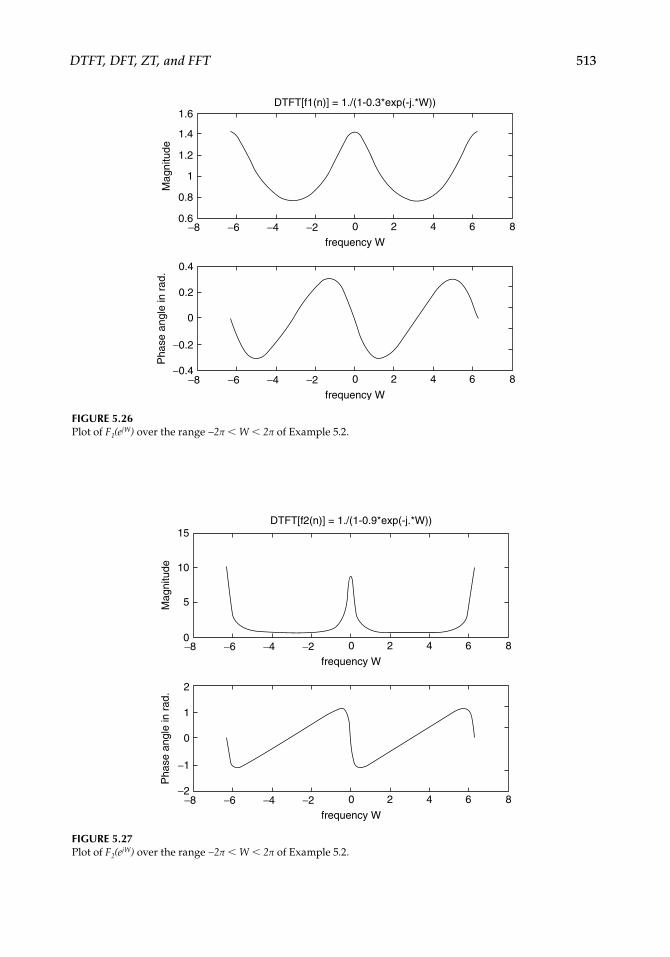
DTFT, DFT, ZT, and FFT 513
−80.6
0.8
1
1.2M
agni
tude
Pha
se a
ngle
in r
ad.
1.4
1.6
−6 −4 −2 0
frequency W
2 4 6 8
−8 −6 −4 −2 0 2 4 6 8−0.4
−0.2
0
0.2
0.4
frequency W
DTFT[f1(n)] = 1./(1-0.3*exp(-j.*W))
FIGURE 5.26Plot of F1(ejW) over the range −2π < W < 2π of Example 5.2.
−80
5
10
Mag
nitu
deP
hase
ang
le in
rad
.
15
−6 −4 −2 0
frequency W
2 4 6 8
−8 −6 −4 −2 0 2 4 6 8−2
−1
0
1
2
frequency W
DTFT[f2(n)] = 1./(1-0.9*exp(-j.*W))
FIGURE 5.27Plot of F2(ejW) over the range −2π < W < 2π of Example 5.2.
CRC_47760_CH005.indd 513CRC_47760_CH005.indd 513 7/23/2008 1:47:32 PM7/23/2008 1:47:32 PM

514 Practical MATLAB® Applications for Engineers
Example 5.3
Let the real sequence h(n) be given by its DTFT as follows:
H ee e e ejW
jW jW jW jW
( ). . . . . .
0 007 0 034 0 04 0 04 0 03 0 0092 3 4 ee
e e e e
j W
jW j W j W j W
5
2 3 41 2 63 2 81 1 5 0 4. . . .
Create the script fi le DTFT_H that returns the magnitude and phase plots of the DTFT of H(ejW) versus W, using 128 discrete points over the range 0 ≤ W ≤ 4π.
MATLAB Solution% Script file: DTFT _ HP = [0.007 0.034 0.04 0.04 0.03 0.009];Q = [1 2.63 2.81 1.5 0.4];W = linspace(0,4*pi,128);H = freqz(P,Q,W);subplot (2,1,1)plot(W,abs(H))title (‘Magnitude of H[exp(jW)] vs. W’)ylabel (‘Magnitude’);xlabel(‘frequency W’);subplot (2,1,2)plot(W,angle(H))title(‘Phase of H[exp(jW)] vs. W’)xlabel(‘frequency W’);ylabel(‘Phase in rad.’)
The script fi le DTFT_H is executed and the results are shown in Figure 5.28.
0 2 4 6 8 100
0.2
0.4
0.6
0.8
1
Mag
nitu
deP
hase
in
rad.
12 14
0 2 4 6 8 10 12 14−4
−2
0
2
4
frequency W
frequency W
Magnitude of H[exp(jW)] versus W
Phase of H[exp(jW)] versus W
FIGURE 5.28Magnitude and phase plots of the DTFT of H(ejW) of Example 5.3.
CRC_47760_CH005.indd 514CRC_47760_CH005.indd 514 7/23/2008 1:47:32 PM7/23/2008 1:47:32 PM

DTFT, DFT, ZT, and FFT 515
Example 5.4
Given the discrete sequence f(n) = [1 2 3],
a. Evaluate by hand the DTF coeffi cients of f(n)
b. Create the script fi le DFT_IDFT that returns the DTF of f(n)
c. Recover the sequence f(n) by evaluating the IDTF of part b
ANALYTICAL Solution
F k f n ej
nkN
n
N
( ) ( )
2
0
1
∑
F f nn
( ) ( )0 1 2 3 60
2
∑
F f n e e e ij
n
n
j j( ) ( ) . .1 1 2 3 1 5000 0 86602
3
0
22 3 4 3
∑
F f n e e e ij
n
n
j j( ) ( ) . .2 1 2 3 1 5000 0 86604
3
0
24 3 8 3
∑
MATLAB Solution% Script file: DFT _ IDFTfn = [1 2 3]DTF _ fn = fft(fn);disp(‘**************** R E S U L T S **************** ’)disp(‘The given time sequence is f(n) = [1 2 3]’)disp(‘The DTF of f(n)=[1 2 3] using fft is given by :’)disp(DTF _ fn)fnn = ifft(DTF _ fn);disp(‘The IDTF of the DFT of f(n)=[1 2 3] using ifft is given by:’)disp(fnn)disp(‘**************************************************** ’)
The script fi le DFT_IDFT is executed and the results are as follows:
******************* R E S U L T S ***********************The given time sequence is f(n) = [1 2 3]The DTF of f(n) = [1 2 3] using fft is given by: 6.0000 -1.5000 + 0.8660i -1.5000 - 0.8660iThe IDTF of the DFT of f(n) = [1 2 3] using ifft is given by: 1 2 3************************************************************
Example 5.5
Create the script fi le DTFT_DFT that returns the magnitude and phase plots of DTFT as well as DFT of the following discrete-time sequence:
f nn
NN
n
k
( ) cos
316
0
1
∑ for
CRC_47760_CH005.indd 515CRC_47760_CH005.indd 515 7/23/2008 1:47:32 PM7/23/2008 1:47:32 PM

516 Practical MATLAB® Applications for Engineers
over the ranges 0 ≤ k ≤ 32 and 0 ≤ k ≤ 64.
MATLAB Solution% Script file: DTFT _ DFTk = linspace(0,16,32);fn32 = cos(3*pi*k/16);kk = linspace(0,16,64);fn64 = cos(3*pi*kk/16);DFT _ fn32 = fft(fn32);DFT _ fn64 = fft(fn64);DFT _ fn = fft(fn32,256);W = 0:1:255;
figure(1)subplot (2,1,1)plot (W,abs(DFT _ fn));title (‘ Magnitudes of the DTFT and DFT’)ylabel (‘Amplitude’)axis ([0 259 0 20])hold onWW= linspace(0,255,32);plot(WW,abs(DFT _ fn32),’*’,WW,abs(DFT _ fn32))axis ([0 259 0 20])subplot (2,1,2)plot (W,abs(DFT _ fn));ylabel (‘Amplitude’)hold onWWW= linspace(0,255,64);plot (WWW,abs(DFT _ fn64),’o’,WWW,abs(DFT _ fn64));xlabel (‘ Index k’);axis([0 259 0 29]);
figure(2)subplot(2,1,1)plot (W,angle(DFT _ fn));title (‘ Phase of the DTFT and DFT’)ylabel (‘Phase angle’)axis ([0 259 -4 4])hold onplot (WW,angle(DFT _ fn32),’*’,WW,angle(DFT _ fn32))subplot (2,1,2)plot (W,angle(DFT _ fn))axis ([0 259 -4 4])hold onplot (WWW,angle(DFT _ fn64),’o’,WWW,angle(DFT _ fn64));axis([0 259 -4 4])ylabel(‘Phase angle’)xlabel(‘Index k’)
The script fi le DTFT_DFT is executed and the results are indicated in Figures 5.29 and 5.30.
CRC_47760_CH005.indd 516CRC_47760_CH005.indd 516 7/23/2008 1:47:33 PM7/23/2008 1:47:33 PM

DTFT, DFT, ZT, and FFT 517
20
15
10
5
00 50 100 150 200 250
0 50 100 150 200 250
DTFT
DTFT
DFT for k = 32
DFT for k = 64
Magnitudes of the DTFT and DFTA
mpl
itude
Am
plitu
de
Index k
0
5
10
15
20
25
FIGURE 5.29Magnitude plots of DTFT and DFT of the discrete sequence f(n) of Example 5.5.
FIGURE 5.30Phase plots of DTFT and DFT of the discrete sequence f(n) of Example 5.5.
0 50 100 150 200 250
0 50 100 150 200 250
Index k
DTFT
DTFT
DFT for k = 64
DFT for k = 32
Phase of the DTFT and DFT4
2
0
−2
−4
4
2
0
−2
−4
Pha
se a
ngle
Pha
se a
ngle
CRC_47760_CH005.indd 517CRC_47760_CH005.indd 517 7/23/2008 1:47:33 PM7/23/2008 1:47:33 PM

518 Practical MATLAB® Applications for Engineers
Example 5.6
Let the input sequence to a system be given by f(n) = [1 0 3 2], and its impulse system response be h(n) = [−1 0 3 4 6 3].
Create the script fi le convolutions that returns
a. The system output g(n)= f(n) ⊗ h(n), using the direct time convolution, as well as the DFT of g(n)
b. The system output g(n) by evaluating the IDFT of the product of the DFT of f(n) with the DFT of h(n)
c. The estimate of the error of the methods used in part a with respect to part b by means of a plot
ANALYTICAL Solution
Note that DFT involves circular convolution, therefore the sequences f(n) and h(n) must be augmented by appending zeros to conform to a length of nine (6 + 4 − 1 = 9) for each sequence.
MATLAB Solution% Script file: convolutionsfn = [1 0 3 2];hn = [-1 0 3 4 6 3];gn = conv(fn,hn); % direct convolutionn = 0:8;fn _ aug = [fn zeros(1,5)];hn _ aug = [hn zeros(1,3)];DTF _ fn _ aug = fft(fn _ aug); % DFTs by zero paddingDTF _ hn _ aug = fft(hn _ aug);DTF _ aug = DTF _ fn _ aug.*DTF _ hn _ aug;ggn = ifft(DTF _ aug); % linear convolution
figure(1)subplot (3,1,1)stem (n,gn); hold on; plot(n,gn); ylabel (‘Amplitude’);xlabel(‘time index n’)title(‘ Linear convolution [g(n)=conv(f(n),h(n))] vs. n’)subplot(3,1,2)DFT _ lin = fft(gn,9);stem (n,abs(DFT _ lin));hold on; plot(n,abs(DFT _ lin));xlabel (‘frequency W’);ylabel(‘Magnitude’);title (‘Magnitude of DFT[g(n)] vs.W’)subplot(3,1,3)stem (n, angle(DFT _ lin)); hold on; plot(n, angle(DFT _ lin));title (‘Phase of DFT[g(n)] vs. W’); xlabel(‘frequency W’)ylabel(‘Angle in rad.’)
figure(2)subplot(3,1,1)
CRC_47760_CH005.indd 518CRC_47760_CH005.indd 518 7/23/2008 1:47:33 PM7/23/2008 1:47:33 PM

DTFT, DFT, ZT, and FFT 519
0 1 2 3 4 5 6 7 8
0 1 2 3 4 5 6 7 8
0 1 2 3 4 5 6 7 8
frequency W
frequency W
Phase of DFT[g(n)] versus W
Magnitude of DFT[g(n)] versus W
Linear convolution [g(n) = conv(f(n), h(n))] versus n
time index n
40
100
50
0
20
Am
plitu
deM
agni
tude
Ang
le in
rad
.
−20
0
5
0
−5
FIGURE 5.31Plots of part a of g(n) and DFT[g(n)] by evaluating the linear convolution of Example 5.6.
stem (n,ggn);hold on; plot(n,ggn); ylabel(‘Amplitude’);xlabel (‘time index n’)title(‘ Circular convolution g(n)=ifft[DTF(f(n)*DTF(h(n)] vs. n’)subplot (3,1,2)DFT _ cir = fft(ggn,9);stem(n,abs(DFT _ cir));hold on; plot(n,abs(DFT _ cir));xlabel(‘frequency W’);ylabel(‘Magnitude’);title(‘Magnitude of DFT[g(n)] vs. W’)subplot (3,1,3)stem(n, angle(DFT _ cir));hold on; plot(n, angle(DFT _ cir));xlabel(‘frequency W’);title (‘Phase of DFT[g(n)] vs. W’);ylabel(‘Angle in rad.’)
figure(3)error = gn-ggn;bar(n,error); title(‘[Errors] vs. time index n’)ylabel (‘Amplitude’)xlabel (‘ time index n’)
The script fi le convolutions is executed and the results are indicated in Figures 5.31 through 5.33.
CRC_47760_CH005.indd 519CRC_47760_CH005.indd 519 7/23/2008 1:47:33 PM7/23/2008 1:47:33 PM

520 Practical MATLAB® Applications for Engineers
[Errors] versus time index n4
× 10−15
2
0
Am
plitu
de
−2
−40 1 2 3 4
time index n
5 6 7 8
FIGURE 5.33Error plot of part a with respect to part b of Example 5.6.
FIGURE 5.32Plots of part b of g(n) and DFT[g(n)] evaluated by circular convolution of Example 5.6.
0 1 2 3 4 5 6 7 8
0 1 2 3 4 5 6 7 8
0 1 2 3 4 5 6 7 8
frequency W
frequency W
Phase of DFT[g(n)] versus W
Magnitude of DFT[g(n)] versus W
Circular convolution g(n)=ifft[DTF(f(n)*DTF(h(n)] versus n
time index n
40
100
50
0
20
Am
plitu
deM
agni
tude
Ang
le in
rad
.−20
0
5
0
−5
CRC_47760_CH005.indd 520CRC_47760_CH005.indd 520 7/23/2008 1:47:33 PM7/23/2008 1:47:33 PM
DTFT, DFT, ZT, and FFT 521
Note that the error in the evaluation of g(n) performed by comparing the linear convo-lution with respect to the circular convolution, is extremely small, in the order of 10−15.
Example 5.7
Let
f n
n
n
n
( )
0 161 16 320 33 64
Create the script fi le rectang that returns the following plots:
a. f(n) versus n
b. The magnitude and phase plots of DFfT[f(n)] versus k, and compare it with the magni-tude and phase plots of DFT[f(n)] versus k, over the ranges 0 ≤ k ≤ 32 and 0 ≤ k ≤ 64
MATLAB Solution% Script file: rectangk = linspace(0,63,64);fn = [zeros(1,16) ones(1,16) zeros(1,32)];DFT _ fn = fft(fn,256);DFT _ fn64 = fft(fn,64);DFT _ fn32 = fft(fn,32);W=0:1:255;
figure(1)plot (k,fn,‘o’,k,fn),axis([0 63 0 1.1]); title(‘ f(n) vs. t’)xlabel (‘time index n’); ylabel(‘Amplitude’)
figure(2)subplot (2,1,1)plot (W,abs(DFT _ fn));title(‘ Magnitudes of the DTFT and DFT’)ylabel(‘Amplitude’)%axis([0 259 0 20])hold onWW=linspace(0,255,32);plot(WW,abs(DFT _ fn32),‘*’,WW,abs(DFT _ fn32))axis([0 259 0 20])subplot(2,1,2)plot(W,abs(DFT _ fn));ylabel(‘Amplitude’)hold onWWW= linspace(0,255,64);plot(WWW,abs(DFT _ fn64),‘o’,WWW,abs(DFT _ fn64));xlabel(‘ Index k’);axis([0 259 0 20]);
figure(3)subplot(2,1,1)plot(W,angle(DFT _ fn));title(‘ Phase of the DTFT and DFT’)ylabel(‘Phase angle’)%axis([0 259 -4 4])hold onplot(WW,angle(DFT _ fn32),‘*’,WW,angle(DFT _ fn32))
CRC_47760_CH005.indd 521CRC_47760_CH005.indd 521 7/23/2008 1:47:34 PM7/23/2008 1:47:34 PM
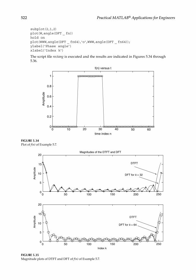
522 Practical MATLAB® Applications for Engineers
20 30
time index n
40 50 601000
0.2
0.4
0.6
Am
plitu
de
0.8
1
f(n) versus t
FIGURE 5.34Plot of f(n) of Example 5.7.
20
15
10
5
0
20
15
10
5
0
0 50 100 150 200 250
0 50 100 150 200 250
DTFT
DFT for k = 32
DFT for k = 64
DTFT
Am
plitu
deA
mpl
itude
Index k
Magnitudes of the DTFT and DFT
FIGURE 5.35Magnitude plots of DTFT and DFT of f(n) of Example 5.7.
subplot(2,1,2)plot(W,angle(DFT _ fn))hold onplot(WWW,angle(DFT _ fn64),‘o’,WWW,angle(DFT _ fn64));ylabel(‘Phase angle’)xlabel(‘Index k’)
The script fi le rectang is executed and the results are indicated in Figures 5.34 through 5.36.
CRC_47760_CH005.indd 522CRC_47760_CH005.indd 522 7/23/2008 1:47:34 PM7/23/2008 1:47:34 PM

DTFT, DFT, ZT, and FFT 523
Example 5.8
Let a communication signal consist of a random noise signal plus an information signal f(t) consisting of three frequencies—1000, 2000, and 3000 Hz.
The noise signal and information signal f(t) are defi ned as follows:
noise = [0 0.5*randn(1, 255)]
f(t) = 0.7sin(2π1000 t) + 0.93cos(2π 2000 t) + 0.69sin(2π3000 t)
Let the communication signal be given by signal(t) = noise + f(t), over the range 0 < t < (1/8000)255, where the sampling period is Ts = (1/8000) s and its sequence length of N = 256.
Create the script fi le signal_n that returns the contaminated signal signal(t) in the time and frequency domains. Observe that in the time domain, the frequencies 1000, 2000, and 3000 Hz are not clearly evident, while in the frequency domain its present is clearly visible.
MATLAB Solution% Script file: signal _ nfs = 8000;Ts =1/fs;N=256;t = linspace(0,Ts*255,256);noise = [0 0.5*randn(1,255)];
0 50 100 150 200 250 300
0 50 100 150 200 250 300
Index k
DTFT
DTFT
4
2
0
−2
−4
4
2
0
−4
−2
DFT for k = 64
DFT for k = 32
Phase of the DTFT and DFTP
hase
ang
leP
hase
ang
le
FIGURE 5.36Phase plots of DTFT and DFT of f(n) of Example 5.7.
CRC_47760_CH005.indd 523CRC_47760_CH005.indd 523 7/23/2008 1:47:34 PM7/23/2008 1:47:34 PM

524 Practical MATLAB® Applications for Engineers
0 0.5−1.5
−1
−0.5
0
0.5
Am
plitu
de
1
1.5
2
1 1.5 2Time
2.5 3 3.5
× 10−3
4
[noise+0.3*sin(2*pi*1000*t)+0.93*cos(2*pi*200*t)+0.69*sin(2*pi*3000*t)] versus t
Communication signal = information + noise
FIGURE 5.37Plot of signal(t) = noise + f(t) of Example 5.8.
signal _ n = noise+0.7*sin(2*pi*1000*t)+0.93*cos(2*pi*2000*t)+0.69*sin (2*pi*3000*t);
figure(1)plot (t(1:33),signal _ n(1:33))title(‘[noise+0.3*sin(2*pi*1000*t)+0.93*cos(2*pi*2000*t)+0.69*sin(2*pi*3000*t)] vs t’)xlabel(‘time’); ylabel(‘Amplitude’);
figure(2)DFT _ mag = abs(fft(signal _ n,256));DFT _ phase = angle(fft(signal _ n,256));subplot (2,1,1)DFTX = DFT _ mag(1:1:128);W = [1:1:N/2].*fs/N;plot (W,DFTX); title(‘DFT Magnitude and Phase’)ylabel (‘Magnitude’);xlabel(‘frequency in Hertz’)subplot (2,1,2)DFTY= DFT _ phase(1:1:128);W = [1:1:N/2].*fs/N;plot (W,DFTY);xlabel(‘frequency in Hertz’); ylabel (‘Angle’)
The script fi le signal_n is executed and the results are indicated in the Figures 5.37 and 5.38.
CRC_47760_CH005.indd 524CRC_47760_CH005.indd 524 7/23/2008 1:47:34 PM7/23/2008 1:47:34 PM

DTFT, DFT, ZT, and FFT 525
Example 5.9
Verify the linearity property of DFT that states, in short, the following:
The sum of DFT[f1(n)] + DFT[f2(n)] + DFT[f3(n)] … is equal to the DFT of the sums of (f1(n) + f2(n) + f3(n) …), for the following specifi c case:
DFT u n DFT u n DFTn
u nn
[ ( )] ( ) cos ( ) 13
7
3
DFT u n u nn
u n nn
( ) ( ) cos ( )13
173
for
16
where
f1(n) = u(n)
f n u nn
2( ) ( )13
f nn
u n3( ) cos ( ) 73
FIGURE 5.38Plots of DFT of signal(t) = noise + f(t) of Example 5.8.
0−4
−2
0
Ang
le
2
4
500 1000 1500 2000
frequency in Hertz
2500 3000 3500 4000
00
50
100
Mag
nitu
de150
500 1000 1500 2000
DFT Magnitude and Phase
frequency in Hertz
2500 3000 3500 4000
CRC_47760_CH005.indd 525CRC_47760_CH005.indd 525 7/23/2008 1:47:35 PM7/23/2008 1:47:35 PM

526 Practical MATLAB® Applications for Engineers
and
f(n) = f1(n) + f2(n) + f3(n)
Create the script fi le linearity that returns the following plots:
a. fi gure(1): [f(n) = f1(n) + f2(n) + f3(n)] versus n, absDFT[f(n)] versus W, and angleDFT[f(n)] versus W (Figure 5.39)
b. fi gure(2): absDFT[f1(n) versus W, absDFT[f2(n) versus W, and absDFT[f3(n) versus W (Figure 5.40)
c. fi gure(3): angleDFT[f1(n) versus W, angleDFT[f2(n) versus W, and angleDFT[f3(n) versus W (Figure 5.41)
d. fi gure(4): Let DFT[f(n)] = DFT[f1(n)] + DFT[f2(n)] + DFT[f3(n)]; obtain plots of absDFT[f(n)] = abs[fft(fn, 16)] and angleDFT[f(n)] = anglefft(fn, 16) (Figure 5.42)
e. fi gure(5): Let us estimate the error in time and frequency by using the following relations (Figure 5.43):
i. The error in time = [f1(n) + f2(n) + f3(n)] − ifftDFT[f(n)] ii. error_magnitude_DFT = absDFT[f1(n) + f2(n) + f3(n)] − absDFT[f1(n)] −
absDFT[f2(n)] − absDFT [f3(n)] iii. error_phase_DFT = angleDFT[f1(n) + f2(n) + f3(n)] − angle[DFT[f1(n)] +
angleDFT[f2(n)] + angleDFT[f3(n)]
MATLAB Solution% Script file: linearityn = 0:1:15;f1n = [ones(1,16)]; % discrete time sequencesf2n = (1/3). n;f3n = 7*cos(n*pi/3);fn = f1n + f2n + f3n;DFT _ fn = fft(fn,16);
figure(1)subplot (3,1,1)stem (n,fn);hold on; stairs(n,fn); ylabel(‘Amplitude’);title(‘ [f(n) = f1(n) + f2(n) + f3(n)] ’)subplot(3,1,2)stem(n,abs(DFT _ fn));hold on; stairs(n,abs(DFT _ fn));ylabel(‘abs [ DFT[f(n)]]’);subplot (3,1,3)stem (n,angle(DFT _ fn));hold on;stairs(n,angle(DFT _ fn));ylabel (‘angle[ DFT [f(n)]]’); xlabel(‘frequency W in rad.’)
figure(2)DFT _ f1= fft(f1n,16); % magnitude of the DFT’s of the discrete sequencesDFT _ f2 = fft(f2n,16);DFT _ f3 = fft(f3n,16);subplot (3,1,1)stem(n,abs (DFT _ f1));hold on; stairs(n,abs(DFT _ f1));ylabel (‘abs [ DFT[f1(n)]]’); title (‘[Magnitudes of the DFTs of f1(n), f2(n) & f3(n)] vs. W ’)
CRC_47760_CH005.indd 526CRC_47760_CH005.indd 526 7/23/2008 1:47:35 PM7/23/2008 1:47:35 PM

DTFT, DFT, ZT, and FFT 527
subplot (3,1,2)stem(n,abs(DFT _ f2));hold on; stairs(n,abs(DFT _ f2));ylabel(‘abs [ DFT[f2(n)]]’);subplot (3,1,3)stem (n, abs(DFT _ f3));hold on;stairs(n,abs(DFT _ f3));xlabel (‘frequency W in rad.’);ylabel(‘abs [ DFT[f3(n)]]’)
figure(3) % phases of the DFT’s of the discrete sequencessubplot(3,1,1)stem (n,angle(DFT _ f1));hold on; stairs (n,angle(DFT _ f1));ylabel (‘angle [ DFT[f1(n)]]’); title (‘[Phases of the DFTs of f1(n), f2(n) & f3(n)] vs. W’)subplot (3,1,2)stem(n,angle(DFT _ f2)); hold on; stairs (n,angle(DFT _ f2));ylabel(‘angle [ DFT[f2(n)]]’);subplot (3,1,3)stem (n, angle(DFT _ f3));hold on;stairs(n,angle(DFT _ f3));xlabel (‘frequency W in rad.’); ylabel(‘angle[ DFT[f3(n)]]’);
figure(4) % magnitude and phase of the sum of DFTsDFT _ fn = DFT _ f1+ DFT _ f2 + DFT _ f3;DFTfn = fft(fn,16);Subplot (2,1,1)stem (n,abs(DFT _ fn)); hold on; stairs(n,abs(DFT _ fn));ylabel (‘abs [ DFT[f(n)] ]’);xlabel(‘frequency W in rad.’);title(‘ DFT[f1(n)] + DFT[f2(n)] + DFT[f3(n)] vs. W’)subplot (2,1,2)stem (n,angle(DFT _ fn));hold on; stairs (n,angle(DFT _ fn));xlabel (‘frequency W in rad.’); ylabel (‘angle [ DFT[fn(n)] ]’);
figure(5) % error analysis in time and frequencyIDFT = ifft(DFT _ fn);error _ time = fn-IDFT;error _ mag _ DFT = abs(DFTfn)-abs(DFT _ fn);error _ phase _ DFT = angle(DFTfn)-angle(DFT _ fn);subplot(3,1,1)bar (n, error _ time);title (‘ Error analysis in time and frequency ‘)ylabel(‘Amplitude in time’)subplot (3,1,2)bar (n,error _ mag _ DFT); ylabel (‘[abs(DFTs)]’);subplot(3,1,3)bar (n,error _ phase _ DFT)ylabel (‘ [angle(DFTs)]’)xlabel (‘frequency W in rad.’);
The script fi le linearity is executed, and the results are shown in Figures 5.39 through 5.43.
CRC_47760_CH005.indd 527CRC_47760_CH005.indd 527 7/23/2008 1:47:35 PM7/23/2008 1:47:35 PM

528 Practical MATLAB® Applications for Engineers
[Magnitude of the DFTs of f1(n), f2(n) & f3(n)] versus W
0 5 10 15
0 5 10 15
0 5 10 15
0
20
abs
[DF
T[f3
(n)]
]ab
s [D
FT
[f2(n
)]]
abs
[DF
T[f1
(n)]
]
40
60
0
0.5
1
1.5
0
10
20
frequency W in rad.
FIGURE 5.40Plots of absDFT of f1(n), f2(n), and f3(n) of Example 5.9.
[f(n) = f1(n) + f2(n) + f3(n)]
0
0
2
0
20
40
60
−10
0
10
−25 10 15
0 5 10 15
0 5 10 15
frequency W in rad.
angl
e [D
FT
[f(n)
]]ab
s [D
FT
[f(n)
]]A
mpl
itude
time index n
W
FIGURE 5.39Plots of [f(n) = f1(n) + f2(n) + f3(n)] and absDFT[f(n)] of Example 5.9.
CRC_47760_CH005.indd 528CRC_47760_CH005.indd 528 7/23/2008 1:47:35 PM7/23/2008 1:47:35 PM

DTFT, DFT, ZT, and FFT 529
151050−2
−1
0
angl
e [D
FT
[fn(n
)]]
1
2
frequency W in rad.
1510500
20
abs
[DF
T[f(
n)]]
40
60
frequency W in rad.
DFT[f1(n)] + DFT[f2(n)] + DFT[f3(n)] versus W
FIGURE 5.42Plots of magnitude and phase angle of the sums of DFT of f1(n), f2(n), and f3(n) of Example 5.9.
FIGURE 5.41Plots of angleDFT of f1(n), f2(n), and f3(n) of Example 5.9.
50
0.5
0
−1
−0.5
2
0
angl
e [D
FT
[f3(n
)]]
angl
e [D
FT
[f2(n
)]]
angl
e [D
FT
[f1(n
)]]
−2
0
1
10 15
50 10 15
50 10frequency W in rad.
15
W
W
[Phases of the DFTs of f1(n), f2(n) & f3(n)] versus W
CRC_47760_CH005.indd 529CRC_47760_CH005.indd 529 7/23/2008 1:47:36 PM7/23/2008 1:47:36 PM

530 Practical MATLAB® Applications for Engineers
Example 5.10
Let the audio analog signal f(t) be given by
f t
t Ts
t Ts t Ts
Ts t Ts( )
cos( )
cos(
0 0 64
7 2 1000 64 128
0 128 192
7
22 1000 192 256 t Ts t Ts)
and sampling rate be Ts = 1/8000 samples/s.Convert the continuous time function f(t) into a discrete sequence f(n).Create the script fi le shift that uses the function f(n) to verify the property that states
that a shift in time only affects the phase spectrum and not the magnitude spectrum by shifting f(n) by 32 time samples and return the following plots:
a. fi gure(1): f(n) versus n, absfft[f(n)] versus f, and anglefft[f(n)] versus f (Figure 5.44)
b. fi gure(2): Repeat part a for f(n − 32) (Figure 5.45)
c. fi gure(3): [error in time = f(n) − f(n − 32)] versus t, [error_mag = absfft[f(n)] − absfft[f(n − 32)]] versus f, and [error_phase = anglefft[f(n)] − anglefft[f(n − 32)]] versus f (Figure 5.46)
d. Estimate the cumulative magnitude and phase errors in the frequency domain
20−2−2
0
2
4 6 8 10 12 14 16
20
0
2
4
−2−2
4 6 8 10 12 14 16
20
0
2
−2 4 6 8frequency W in rad.
10 12 14 16
Error analysis in time and frequency
Am
plitu
de in
tim
e[a
bs(D
FT
s)]
[ang
le(D
FT
s)]
time index n
W
× 10−15
× 10−15
× 10−15
FIGURE 5.43Time and frequency error plots of Example 5.9.
CRC_47760_CH005.indd 530CRC_47760_CH005.indd 530 7/23/2008 1:47:36 PM7/23/2008 1:47:36 PM

DTFT, DFT, ZT, and FFT 531
MATLAB Solution% Script file: shiftN=256; fs = 8000;Ts =1/fs; shift =32;t = linspace(0,Ts*255,256);window = [zeros(1,64) ones(1,64) zeros(1,64) ones(1,64)];f = 7*cos(2*pi*1000*t);fn=f.*window;DFT _ fn = fft(fn,256);fn _ shift = 7*cos(2*pi*1000*(t-shift).*window);DFT _ fn _ shift = fft(fn _ shift,256);
figure(1)subplot (3,1,1); % analysis of f(n) = 7cos(2.pi.1000.t)*windowplot (t,fn); ylabel(‘Magnitude’);title (‘f(n) = 7cos(2.pi.1000.n)*window, analyzed in the time and
frequency domains’)subplot (3,1,2)W= [1:1:N/2].*fs/N;DFT _ mag = abs(DFT _ fn);DFT _ phase = angle(DFT _ fn);DFT _ mage = DFT _ mag(1:1:128);DFT _ phasee = DFT _ phase(1:1:128);plot(W,DFT _ mage); ylabel(‘abs [ DFT[f(n)]]’);subplot (3,1,3)plot (W,DFT _ phasee);ylabel (‘angle[ DFT [f(n)]]’); xlabel (‘ frequency in Hz’)
figure(2); % Analysis of 7cos(2.pi.(n-shift))DFT _ mags = abs(DFT _ fn _ shift);DFT _ phases = angle(DFT _ fn _ shift);DFT _ magess = DFT _ mag(1:1:128);DFT _ phasess =DFT _ phase(1:1:128);subplot (3,1,1)plot (t,fn _ shift); title(‘ f(n-32) analyzed in the time and frequency domains’)ylabel(‘Amplitude in time’);subplot(3,1,2)plot(W,DFT _ magess);ylabel(‘Magnitude DFT[f(n-32)]’);subplot(3,1,3)plot(W,DFT _ phasess);xlabel(‘frequency in Hz ’); ylabel(‘Phase of DFT[f(n-32)]’);
figure(3) % error analysis subplot(3,1,1)error _ time = fn-fn _ shift;plot(t, error _ time);title(‘ Error analysis in the time and frequency domains ’)ylabel(‘Magnitude in time’)subplot(3,1,2)error _ mag=abs(DFT _ fn)-abs(DFT _ fn _ shift);bar(W,abs(error _ mag(1:128)));ylabel(‘Magnitude ’);subplot(3,1,3)error _ phase=angle(DFT _ fn)-angle(DFT _ fn _ shift);bar(W,abs(error _ phase(1:128)));ylabel(‘Phase ’);
CRC_47760_CH005.indd 531CRC_47760_CH005.indd 531 7/23/2008 1:47:36 PM7/23/2008 1:47:36 PM

532 Practical MATLAB® Applications for Engineers
xlabel(‘frequency in Hz’)disp(‘*******************************************************************’)disp(‘********************** R E S U L T S ****************************’)fprintf(‘For a shift of:%f\n’,shift);error _ mag _ DFT= sum(abs(DFT _ fn)-abs(DFT _ fn _ shift));error _ phase _ DFT=sum(angle(DFT _ fn)-angle(DFT _ fn _ shift));fprintf(‘Cumulative magnitude of the error in the frequency domain:%f\n’,error _ mag _ DFT);fprintf(‘Cumulative phase error in the frequency domain:%f\n’,error _ phase _ DFT);disp(‘*******************************************************************’)
The script fi le shift is executed, and the results are as follows:
>> shift
*************************************************************************************************** R E S U L T S *******************************For a shift of: 32.000000Cumulative magnitude of the error in the frequency domain:-2245.168919Cumulative phase error in the frequency domain:3.141593*************************************************************************
Time
0 500 1000 1500 2000
frequency in Hz
Frequency
2500 3000 3500 4000
0 500 1000 1500 2000 2500 3000 3500 4000
5
0
200
400
600
−10
0
0 0.005 0.01 0.015 0.02 0.025 0.03 0.035
10
0
angl
e [D
FT
[f(n)
]]ab
s [D
FT
[f(n)
]]M
agni
tude
−5
f(n)=7cos(2.pi.1000.n)*window, analyzed in the time and frequency domains
FIGURE 5.44Plots of f(n) in time and frequency of Example 5.10.
CRC_47760_CH005.indd 532CRC_47760_CH005.indd 532 7/23/2008 1:47:36 PM7/23/2008 1:47:36 PM

DTFT, DFT, ZT, and FFT 533
Time
0 500 1000 1500 2000frequency in Hz
Frequency
2500 3000 3500 4000
0 500 1000 1500 2000 2500 3000 3500 4000
5
0
200
400
600
−10
0
0 0.005 0.01 0.015 0.02 0.025 0.03 0.035
10
0
Pha
se o
f D
FT
[f(n-
32)]
Mag
nitu
de
DF
T[f(
n-32
)]A
mpl
itude
in ti
me
−5
f(n-32) analyzed in the time and frequency domains
FIGURE 5.45Plots of f(n − 32) in time and frequency of Example 5.10.
Error analysis in the time and frequency domains
0
1000
500
00 500 1000 1500 2000 2500 3000 3500 4000 4500
00
2
4
6
500 1000 1500 2000 2500
frequency in Hz
3000 3500 4000 4500
−10
−5
0
5
0.005 0.01 0.015 0.02 0.025 0.03 0.035
Pha
seM
agni
tude
Mag
nitu
de in
tim
e
Time
Frequency
FIGURE 5.46Error plots in time and frequency of Example 5.10.
CRC_47760_CH005.indd 533CRC_47760_CH005.indd 533 7/23/2008 1:47:37 PM7/23/2008 1:47:37 PM

534 Practical MATLAB® Applications for Engineers
Observe that the magnitude spectrum for f(n) and f(n − 32) are similar. The phase-error plot shows variations that are proportional to the shift (32). Note that the error in time is large; but in frequency, approximately 1000 Hz, the magnitude and phase errors are small.
Example 5.11
This example explores and verifi es some properties that relate the correlation with the convolution process.
Let f1(n) = sin(2πn/16) and f2(n) = cos(2πn/16), over the range n = 0, 1, 2, 3, 4, …, 16.Create the script fi le conv_corr that returns the following:
a. fi gure(1): f1(n) versus n and f2(n) versus n, over the range 0 ≤ n ≤ 31, using the stairs command
b. fi gure(2), explore the conv and xcorr functions in time by obtaining and comparing the following plots:
i. [corr = xcorr(f1n, f2n)] versus n ii. [conv1 = conv(f1n, f2(−n))] versus n iii. [conv2 = conv(f1(−n), f2n)] versus n
c. fi gure(3) verifi es that the maximum point occurs at the midrange, and this point corresponds to R11(0) and R22(0), by obtaining the following plots:
i. [R11 = aut_corr1 = xcorr(f1n, f1n)] versus n ii. [R1 = aut_xcorr(f1n)] versus n iii. [R22 = aut_corr2 = xcorr(f2n, f2n)] versus n
Observe that R1 ≠ R22, but R11 = R22. d. fi gure(4), normalized frequency analysis (verify that the two following plots are
identical) i. abs[conj[fft(f1n)] * fft(f2n)] versus W ii. abs[fft(xcorr(f1(n), f2(n)))] versus W
e. fi gure(5), error analysis in time i. [error1(n) = xcorr(f1(n), f2(n)) − conv(f1(n), f2(−n))] versus n and ii. [error2(n) = abs(abs(xcorr(f1(n), f2(n))) − abs(conv(f1(−n), f2(n))))] versus n
MATLAB Solution% Script file: conv _ corrn=0:1:31;f1n=sin(2*pi*n./16);f2n=cos(2*pi*n./16);f1n _ rev=fliplr(f1n);f2n _ rev=fliplr(f2n);
figure(1) % discrete time plots of f1(n) and f2(n)subplot(2,1,1)stairs(n,f1n), axis([0 33 -1.1 1.1]),title(‘ Stair plot of f1(n) vs. n’);ylabel(‘Amplitude ’);subplot(2,1,2)stairs(n,f2n); axis([0 33 -1.1 1.1]),title(‘ Stair plot of f2(n) vs. n’);xlabel(‘time index n’);ylabel(‘Amplitude’);
CRC_47760_CH005.indd 534CRC_47760_CH005.indd 534 7/23/2008 1:47:37 PM7/23/2008 1:47:37 PM

DTFT, DFT, ZT, and FFT 535
figure(2)corr = xcorr(f1n,f2n);N= length (corr);m = 0:1:N-1;subplot (3,1,1)stem(m,corr);title(‘Convolution and correlation plots’);ylabel(‘Amplitude’);subplot(3,1,2)conv1=conv(f1n,f2n _ rev);stem(m,conv1)xlabel(‘time index n’);ylabel(‘Amplitude’);subplot(3,1,3)conv2=conv(f1n _ rev,f2n);stem(m,conv2);xlabel(‘time index n’);ylabel(‘Amplitude’);
figure(3) % auto-correlationsmm=-31:31;aut _ corr1=xcorr(f1n,f1n);aut=xcorr(f1n);aut _ corr2=xcorr(f2n,f2n);plot(mm,aut _ corr1,mm,aut _ corr2,mm,aut); title(‘Auto-correlation plots’);ylabel(‘Amplitude’);legend(‘R11’,’R22’,’R1’)
figure(4) % frequency analysisDFT _ corr = fft(corr,256);DFT _ f1n = fft(f1n,256);DFT _ f2n = fft(f2n,256);DFT _ 12 = conj(DFT _ f1n).*DFT _ f2n;k=1:1:256;subplot (2,1,1)plot (k/256,abs(DFT _ 12));title(‘abs[conj[fft(f1n)]*fft(f2n)] vs. W ’)ylabel(‘Magnitude’)subplot(2,1,2)plot(k/256,abs(DFT _ corr));title(‘abs[fft(xcorr(f1(n),f2(n)))] vs. W’)xlabel(‘W’); ylabel(‘Magnitude’)
figure(5)subplot (2,1,1)error1 = corr-conv1;bar(m,error1);title(‘error1=corr[f1(n),f2(n)]-conv[f1(n),f2(-n)]’)ylabel(‘Amplitude’);subplot(2,1,2)error2 = abs(abs(corr)-abs(conv2));bar(m,error2)title (‘error2=abs[abs[corr[f1(n),f2(n)]]-abs[conv[f1(-n),f2(n)]]]’)xlabel (‘time index n’); ylabel(‘Amplitude’)
The script fi le conv_corr is executed, and the results are as follows:
>> conv _ corr
CRC_47760_CH005.indd 535CRC_47760_CH005.indd 535 7/23/2008 1:47:37 PM7/23/2008 1:47:37 PM

536 Practical MATLAB® Applications for Engineers
1
0.5
0
0 5 10 15
Stair plot of f1(n) versus n
20 25 30
Am
plitu
de
−0.5
−1
1
0.5
0
0 5 10 15
time index n
Stair plot of f2(n) versus n
20 25 30
Am
plitu
de
−0.5
−1
FIGURE 5.47Plots of f1(n) and f2(n) of Example 5.11.
20
0
−200 10 20 30 40 50 60 70
20
0
−200 10 20 30 40 50 60 70
20
0
−200 10 20 30 40 50 60 70
time index n
time index n
time index n
Am
plitu
deA
mpl
itude
Am
plitu
de
Convolution and correlation plots
[xcross(f1(n), f2(n))] versus n
[conv(f1(n), f2(-n))] versus n
[conv((f1(-n), f2(n))] versus n
FIGURE 5.48Convolution and correlation plots of part b of Example 5.11.
See Figures 5.47 through 5.51.
CRC_47760_CH005.indd 536CRC_47760_CH005.indd 536 7/23/2008 1:47:37 PM7/23/2008 1:47:37 PM

DTFT, DFT, ZT, and FFT 537
−15−40 −30 −20 −10 0 10 20 30 40
−10
−5
0
Am
plitu
de
5
10
15
20Auto-correlation plots
R11R22R1
FIGURE 5.49(See color insert following page 374.) Autocorrelation plots of part c of Example 5.11.
abs[conj[fft(f1n)]*fft(f2n)] versus W
abs[fft(xcorr(f1(n),f2(n)))] versus W
00
100
200
Mag
nitu
de
300
0.1 0.2 0.3 0.4 0.5 0.6 0.7 0.8 0.9 1
00
100
200
Mag
nitu
de
300
0.1 0.2 0.3 0.4 0.5W
0.6 0.7 0.8 0.9 1
FIGURE 5.50Plots of part d—abs[conj[fft(f1n)] * fft(f2n)] and abs[fft(xcorr(f1(n), f 2(n)))]—of Example 5.11.
CRC_47760_CH005.indd 537CRC_47760_CH005.indd 537 7/23/2008 1:47:38 PM7/23/2008 1:47:38 PM

538 Practical MATLAB® Applications for Engineers
20 30
time index n
40 50 60 701000
0.5
1
1.5
−10
20 30 40 50 60 70100−10−4
−2
0
Am
plitu
deA
mpl
itude
2
4
6× 10⁻¹⁵
error2 = abs[abs[corr[f1(n), f2(n)]]-abs[conv[f1(-n), f2(n)]]]
error1 = corr[f1(n), f2(n)]-conv[f1(n), f2(-n)]
FIGURE 5.51Error plots of part e of Example 5.11.
Example 5.12
The objective of this example is to explore the relation between the FT of a continuous time function and its discrete version.
Let f(t) = 3e−5tu(t).Create the script fi le FT_DFT that returns the following plots:
a. f(t) versus t, over the range 0 ≤ t ≤ 1 (Figure 5.52)
b. Magnitude and phase of [DFT[f(n)]] versus w (Figure 5.53)
c. Magnitude and phase of [FT[f(t)]] versus w (Figure 5.54)
d. error_mag = magnitude of [FT[f(t)]] − magnitude of [DFT[f(n)]] versus w and error_phase = phase of [FT[f(t)]] − phase of [DFT[f(n)]] versus w (Figure 5.55)
MATLAB Solution% Script file: FT _ DFTN = 526;t = linspace(0,5,N);fn =3*exp(-5*t); fs = 8000;Ts = 1/fs;ws = 2*pi/Ts;F = fft(fn);Fdc = fftshift(F)*Ts;W = ws*(-N/2:(N/2)-1)/N;
figure(1)plot (t(1:100),fn(1:100));title (‘[f(t)=3*exp(-5*t)] vs t’)ylabel (‘Amplitude’); xlabel (‘time’);axis([0 1 0 3.5]);
figure(2) % discrete frequency analysissubplot (2,1,1)plot (W,abs(Fdc));title(‘abs[DFT[f(n)]] vs w’);ylabel(‘Magnitude’);
CRC_47760_CH005.indd 538CRC_47760_CH005.indd 538 7/23/2008 1:47:38 PM7/23/2008 1:47:38 PM

DTFT, DFT, ZT, and FFT 539
00
0.5
1
1.5Am
plitu
de 2
2.5
3
3.5
0.1 0.2 0.3 0.4 0.5 0.6
time
0.7 0.8 0.9 1
[f(t)=3*exp(-5*t)] versus t
FIGURE 5.52Plot of f(t) over the range 0 ≤ t ≤ 1 of Example 5.12.
axis([-1e4 1e4 0 0.01])subplot (2,1,2)plot (W,angle(Fdc));title(‘angle[DFT[f(n)]] vs w’);ylabel(‘Phase’);xlabel (‘frequency w ’);
figure(3) % analog frequency analysisF _ table = 3./(5+j*W);subplot (2,1,1)absF _ table = abs(F _ table);plot(W(200:400),absF _ table(200:400));title(‘abs[FT[f(t)]] vs w’);ylabel(‘Magnitude’);axis([-.1e4 .1e4 0 0.8]);subplot (2,1,2)plot (W,angle(F _ table));title(‘angle[FT[f(t)]] vs w’);ylabel(‘Phase’);xlabel (‘frequency w ‘);axis([-1e4 1e4 -2 2]);
figure(4) % error analysis in frequencyerror _ mag = abs(F _ table)-abs(Fdc);error _ phase = angle(F _ table)-angle(Fdc);subplot (2,1,1)plot (W(200:400) ,error _ mag(200:400));axis([-.2e4 .2e4 0 0.8]);title (‘error mag.=abs[FT[f(t)]]-abs[DFT[f(n)]] vs w n’);ylabel (‘Magnitude’); xlabel (‘index n’)subplot(2,1,2)bar(W,error _ phase);title(‘error phase=angle[FT[f(t)]-angle[DFT[f(n)]]
vs w’);ylabel(‘Phase’);xlabel(‘frequency w’);
The script fi le FT_DFT is executed, and the results are as follows:
>> FT _ DFT
CRC_47760_CH005.indd 539CRC_47760_CH005.indd 539 7/23/2008 1:47:39 PM7/23/2008 1:47:39 PM

540 Practical MATLAB® Applications for Engineers
−3−2
−1
0
Pha
se
1
2
0
0.002
0.004
Mag
nitu
de 0.006
0.008
0.01
−2 −1
−1 −0.8 −0.6 −0.4 −0.2 0 0.2
angle[DFT[f(n)]] versus w
abs[DFT[f(n)]] versus w
0.4 0.6 0.8 1
0 1 2 3frequency w × 104
× 104
FIGURE 5.53Plot of DFT[f(n)] of Example 5.12.
−1
−1000 −800
0.8
0.6
0.4
Mag
nitu
de
0.2
0−600 −400 −200 0
angle[FT[f(t)]] versus w
abs[FT[f(t)]] versus w
200 400 600 800 1000
−2
−1
0
Pha
se
1
2
−0.8 −0.6 −0.4 −0.2 0
frequency w × 104
0.2 0.4 0.6 0.8 1
FIGURE 5.54Plot of FT[ f(t)] of Example 5.12.
CRC_47760_CH005.indd 540CRC_47760_CH005.indd 540 7/23/2008 1:47:39 PM7/23/2008 1:47:39 PM

DTFT, DFT, ZT, and FFT 541
Example 5.13
The system difference equation of an LTI system is given by
g(n) = 0.7g(n − 1) − 0.3g(n − 2) + f(n) + 0.9f(n − 1)
a. Determine by hand the discrete-transfer function H(z) = G(z)/F(z).
b. Determine by hand H(ejW). c. Obtain the plots of the input f(n) versus n and output gf (n) versus n at steady
state (Figure 5.56), over the range 1 ≤ n ≤ 50, assuming that the input is f(n) = (0.5)nsin(0.033πn)u(n), using the MATLAB command fi lter.
d. Obtain the plot of the impulse response h(n) by using the MATLAB command impz and g(n) by using convolution (Figure 5.57), over the range 1 ≤ n ≤ 50. Let gc(n) denote the convolution of h(n) with f(n) (time domain) and gf (n) be the system out-put obtained by the fi lter command (frequency domain).
e. Evaluate and plot the magnitude and phase of fft[gf (n)] and fft[gc(n)], over the range 1 ≤ k ≤ 50 (Figure 5.58).
f. Estimate and plot (Figure 5.59) the error of the above two methods (gf (n) and gc (n)) in the time domain defi ned by the following relation:
error(n) = gf (n) – gc(n), over 1 ≤ n ≤ 50
−2000 −15000
0.2
0.4
Mag
nitu
de0.6
0.8
−1000 −500 0Index n
500 1000 1500 2000
2
1
Pha
se 0
−1
−2−3 −2 −1 0
frequency w1 2 3
× 104
error mag.=abs[FT[f(t)]]-abs[DFT[f(n)]] versus w
error phase=angle[FT[f(t)]]-angle[DFT[f(n)]] versus w
FIGURE 5.55Error plot of FT[ f(n)] with respect to DFT[ f(n)] of Example 5.12.
CRC_47760_CH005.indd 541CRC_47760_CH005.indd 541 7/23/2008 1:47:39 PM7/23/2008 1:47:39 PM

542 Practical MATLAB® Applications for Engineers
g. Estimate and plot (Figure 5.59) the magnitude and phase errors of the two methods in the frequency domain defi ned by the following relations:
mag_error = absfft[gf (n)] − absfft[gc(n)]
phase_error = anglefft[gf (n)] − anglefft[gc(n)]
over the range 1 ≤ k ≤ 50.
The MATLAB solution for Example 5.13 is given by the script fi le discrete_syst as follows:
ANALYTICAL Solution
Part a
g(n) = 0.7g(n − 1) − 0.3g(n − 2) + f(n) + 0.9f(n − 1)
g(n) − 0.7g(n − 1) + 0.3g(n − 2) = f(n) + 0.9f(n − 1)
Taking the ZT yields
G(z) − 0.7z−1G(z) + 0.3z−2G(z) = F(z) + 0.9z−1F(z)
G(z)[1 − 0.7z−1 + 0.3z−2] = F(z)[1 + 0.9z−1]
H zz
z z( )
1 0 91 0 7 0 3
1
1 2
.. .
Part b
Replacing z = ejW
H eG eF e
ee e
jWjW
jW
jW
jW j W( )
( )( )
.. .
1 0 91 0 7 0 3 2
MATLAB Solution% Script file: discrete _ systnum = [1 0.9];den = [1 -0.7 0.3];n = 1:1:50;fn = 0.9. n.*sin(0.033*pi.*n);gnf = filter(num,den,fn);
figure(1) % input and output plotssubplot(2,1,1)plot(n,fn,’o’,n,fn); title(‘[System input sequence f(n)] vs n’)xlabel(‘time index n’);ylabel(‘Magnitude’)subplot(2,1,2)plot(n,gnf,’s’,n,gnf);
CRC_47760_CH005.indd 542CRC_47760_CH005.indd 542 7/23/2008 1:47:39 PM7/23/2008 1:47:39 PM

DTFT, DFT, ZT, and FFT 543
title(‘[System output sequence g(n)] vs n, using filter’) xlabel(‘time index n’);ylabel(‘Magnitude’)
figure(2) % impulse analysishn = impz(num,den,n);subplot (2,1,1)stem(n,hn);title(‘ [System impulse response h(n)] vs n, using impz’)ylabel(‘Amplitude’); xlabel(‘time index n’)subplot(2,1,2)nn=0:1:50;gnc=conv(hn,fn);stem(nn(1:1:50),gnc(1:1:50))title(‘ [System output g(n)] vs n, using convolution’)ylabel(‘Amplitude’);xlabel(‘time index n’)
figure(3) % frequency analysisDFT _ gnf = fft(gnf); abs _ DFT _ gnf = abs(DFT _ gnf); ang _ DFT _ gnf=angle(DFT _ gnf);DFT _ gnc = fft(gnc);abs _ DFT _ gnc=abs(DFT _ gnc);ang _ DFT _ gnc=angle(DFT _ gnc);subplot(2,2,1); stem(nn(1:1:50),abs _ DFT _ gnf(1:1:50));ylabel(‘abs[fft(gf(n))]’);title(‘abs[fft(gf(n))] vs k’)axis([0 50 0 20]);subplot(2,2,2)stem(nn(1:1:50),ang _ DFT _ gnf(1:1:50));title(‘angle[fft(gf(n))] vs k’);ylabel(‘angle[fft(gf(n))]’);axis([0 50 -4 4]);subplot(2,2,3);stem(nn(1:1:50),abs _ DFT _ gnc(1:1:50));title(‘abs[fft(gc(n))] vs k’);xlabel(‘index k’);ylabel(‘abs[fft(gc(n))]’);axis([0 50 0 20])subplot(2,2,4)stem(nn(1:1:50),ang _ DFT _ gnc(1:1:50));title(‘angle[fft(gc(n))] vs k’);xlabel(‘index k’);ylabel(‘angle[fft(gc(n))]’);axis([0 50 -4 0])
figure(4) % error analysissubplot(3,1,1)error _ time = gnf(1:1:50)-gnc(1:1:50);bar(nn(1:1:50),error _ time);axis([0 50 -0.5 0.5]);title(‘ error plots in time and frequency’)ylabel(‘Amplitude’)subplot(3,1,2) mag _ error = abs _ DFT _ gnf(1:1:50)- abs _ DFT _ gnc(1:1:50);phase _ error = ang _ DFT _ gnf(1:1:50)- ang _ DFT _ gnc(1:1:50);bar(nn(1:1:50),mag _ error); ylabel(‘Magnitude error’)axis([0 50 -10 10])subplot(3,1,3)bar(nn(1:1:50),phase _ error);ylabel(‘phase error’);axis([0 50 -10 10]); xlabel(‘index k’);
The script fi le discrete_syst is executed, and the results are as follows:
>> discrete _ syst
CRC_47760_CH005.indd 543CRC_47760_CH005.indd 543 7/23/2008 1:47:40 PM7/23/2008 1:47:40 PM

544 Practical MATLAB® Applications for Engineers
0 5 10 15 20 25 30 35 40 45 50−1
0
1
2 [System impulse response h(n)] versus n, using impz
Am
plitu
de
time index n
0 5 10 15 20 25 30 35 40 45 50−0.5
0
0.5
1 [System output g(n)] versus n, using convolution
Am
plitu
de
time index n
FIGURE 5.57Plots of system impulse h(n) and system output gc(n) of Example 5.13.
0 5 10 15 20 25 30 35 40 45 50
0
0.2
0.4
0.6[System input sequence f(n)] versus n
time index n
Mag
nitu
de
0 5 10 15 20 25 30 35 40 45 50−0.5
−0.2
0
0.5
1
1.5[System output sequence g(n)] versus n, using filter
time index n
Mag
nitu
de
FIGURE 5.56Plots of the system input f(n) and system output gf (n) of Example 5.13.
CRC_47760_CH005.indd 544CRC_47760_CH005.indd 544 7/23/2008 1:47:40 PM7/23/2008 1:47:40 PM

DTFT, DFT, ZT, and FFT 545
0 10 20 30 40 500
5
10
15
20
abs[
fft(g
f(n)
)]
abs[fft(gf(n))] versus k
0 10 20 30 40 50−4
−2
0
2
4angle[fft(gf(n))] versus k
angl
e[fft
(gf(
n))]
0 10 20 30 40 500
5
10
15
20abs[fft(gc(n))] versus k
index k
abs[
fft(g
c(n)
)]
0 10 20 30 40 50−4
−3
−2
−1
0angle[fft(gc(n))] versus k
index k
angl
e[fft
(gc(
n))]
FIGURE 5.58Magnitude and phase plots of fft[gf (n)] and fft[gc(n)], over the range 1 ≤ k ≤ 50 of Example 5.13.
0 5 10 15 20 25 30 35 40 45 50−0.5
0
0.5 error plots in time and frequency
Am
plitu
de
0 5 10 15 20 25 30 35 40 45 50−10
−10
10
0
Mag
nitu
de e
rror
0 5 10 15 20 25 30 35 40 45 50
0
10
phas
e er
ror
index k
index n
error = g(n)<using filter> - g(n)<using convolution>
∠error(k) = ∠DFT[gf(n)] - ∠DFT[gf(n)]
error = DFT[g(n)<filter> - DFT[g(n)<convolution>]
FIGURE 5.59Error plots in the time and frequency domains of Example 5.13.
CRC_47760_CH005.indd 545CRC_47760_CH005.indd 545 7/23/2008 1:47:41 PM7/23/2008 1:47:41 PM

546 Practical MATLAB® Applications for Engineers
Example 5.14
Let the impulse response of an LTI system be given by h n n
n( ) .
0 50
15∑ and the system
input sequence be f n nn
( ) cos( / )
15 5 30
15∑
.Create the script fi le syst_anal that returns the following plots:
a. f(n) versus n and h(n) versus n, using the stem command (Figure 5.60)
b. g(n) = IDFT of the products of DFT [f(n)] times DFT [h(n)] versus n (Figure 5.61)
c. gnn(n) = convolution of h(n) with g(n) versus n (Figure 5.61)
d. Estimate the error plot (in the time domain) of the two approaches (parts b and c), given by (Figure 5.62)
error(n) = [g(n) − gnn(n)] versus n
MATLAB Solution% Script file: syst _ analn = 0:15;fn = cos(5*pi*n/3);hn = 0.5. n; % the length of convolution is 16*2-1DFT _ F = fft(fn,31);DFT _ H = fft(hn,31);gn = ifft(DFT _ F.*DFT _ H);
figure(1)subplot(2,1,1)stem(n,fn)ylabel(‘Amplitude’);axis([0 15 -1.2 1.2]);title(‘ [Input sequence f(n)] vs n ‘)subplot(2,1,2)stem(n,hn)ylabel(‘Amplitude ‘);axis([0 15 -0.5 1.2]);xlabel(‘time index n’); title(‘[Impulse response h(n)] vs n’)
figure(2) % output plotssubplot(2,1,1)nn=0:1:30;plot(nn,gn);title(‘[IDFT of the products of the DFTs ] vs n’);xlabel(‘time index n ’); ylabel(‘Amplitude’);axis([0 25 -1.5 2]);subplot(2,1,2)gnn=conv(fn,hn);plot(nn,gnn);axis([0 25 -1.5 2]);xlabel(‘time index n’), ylabel(‘Amplitude’)title(‘[Direct convolution in the time domain] vs. n’);
figure(3)error = gn-gnn;bar(nn,error);title(‘ Error =[part(b)-part(c)] vs. n’ );xlabel(‘time index n’), ylabel(‘Magnitude’);
The script fi le syst_anal is executed, and the results are as follows:
>> syst _ anal
CRC_47760_CH005.indd 546CRC_47760_CH005.indd 546 7/23/2008 1:47:41 PM7/23/2008 1:47:41 PM

DTFT, DFT, ZT, and FFT 547
0 5 10time index n
15 20 25
0 5 10time index n
15 20 25
Am
plitu
de
−1
0
1
2
Am
plitu
de
−1
0
1
2[IDFT of the products of the DFTs] versus n
[Direct convolution in the time domain] versus n
FIGURE 5.61Plots of g(n) = IDFT of the products of DFT[h(n)] with DFT[ f (n)], and time convolution of h(n) with f(n) of Exam-ple 5.14.
0 5 10
[Impulse response h(n)] versus n
[Input sequence f(n)] versus n
15
0 5 10 15
time index n
Am
plitu
de
−0.5
0
0.5
1
Am
plitu
de
−1
−0.5
0
0.5
1
FIGURE 5.60Plots of f(n) and h(n) of Example 5.14.
CRC_47760_CH005.indd 547CRC_47760_CH005.indd 547 7/23/2008 1:47:41 PM7/23/2008 1:47:41 PM

548 Practical MATLAB® Applications for Engineers
Error = [part(b)-part(c) versus n
6
8× 10⁻¹⁶
4
2
0
−2
−4
−6−5 0 5 10 15 20 25 30 35
time index n
Am
plitu
de
FIGURE 5.62Time-domain error given by error = part b − part c of Example 5.14.
Example 5.15
Create the script fi le analys that analyzes the discrete system transfer function given by
H eG eF e
e ee e
jWjW
jW
jW jW
jW j W( )
( )( )
.. .
5 0 91 0 7 0 3
2
2
and returns the following:
a. The pole/zero plot of H(ejW) (evaluates the system stability) (Figure 5.63)
b. The plot of absH(ejW) versus W (Figure 5.64)
c. The plot of angle H(ejW) versus W
d. List all the poles, zeros, and stand alone term of the transfer function H(z=ejW) and compare the results obtained with the results of part a
e. Determine the ROC of H(z = ejW)
f. The magnitude of the system poles (length from origin)
g. The partial fraction expansion of H(z)
h. h(n) by using the symbolic MATLAB inverse ZT of H(z)
MATLAB Solution%Script file = analysnum = [5 0.9 1];den = [1 -0.7 0.3];
figure(1)zplane(num,den); title(‘Pole and zero plot of H(z)’)
figure(2)W = -pi:pi/99:pi;[H,W] = freqz(num,den,W);
CRC_47760_CH005.indd 548CRC_47760_CH005.indd 548 7/23/2008 1:47:42 PM7/23/2008 1:47:42 PM

DTFT, DFT, ZT, and FFT 549
magH = abs(H);phaseH = angle(H);subplot (2,1,1);plot (W,magH);title (‘abs[H(exp(-jW))] vs W’);ylabel(‘Magnitude’);subplot (2,1,2);plot (W,phaseH);title(‘angle[H(exp(-jW))] vs W’);ylabel (‘Phase in rad.’);xlabel(‘frequency W in rad’);[z,p,k] = tf2zp(num,den);m = abs(p);disp(‘*****************************************’);disp(‘************ R E S U L T S *************’);disp(‘*****************************************’)disp(‘The zeros of H(z) are:’);disp(z);disp(‘The poles of H(z) are:’);disp(p);disp(‘The gain of H(z) is:’);disp(k);disp(‘The magnitude of the poles are:’);disp(m);disp(‘The ROC is outside the circle with radius:’);disp(max(m))% partial fraction expansion[r,pp,kk] = residuez (num,den);disp(‘Partial fraction coefficients of H(z)’)disp(‘the residues are:’)disp(r);disp(‘the stand alone term is :’);disp(kk);syms z Fz;disp(‘The partial fraction expansion is:’)Fz = r(1)/(z-pp(1))+r(2)/(z-pp(2))+ kkhn = iztrans(Fz);disp(‘The impulse response h(n) is:’);hndisp(‘ ^^^^^^^^^^^^^^^^^^^^^^^^^^^^^^^^^^^^^^^^^^ ’)
The script fi le analys is executed, and the results are as follows:
>> analys
***************************************************** R E S U L T S ******************************************************
The zeros of H(z) are: -0.0900 + 0.4381i -0.0900 - 0.4381iThe poles of H(z) are: 0.3500 + 0.4213i 0.3500 - 0.4213i
The gain of H(z) is: 5The magnitude of the poles are: 0.5477 0.5477The ROC is outside the circle with radius: 0.5477Partial fraction coefficients of H(z)the residues are: 0.8333 - 4.5295i 0.8333 + 4.5295i
the stand alone term is: kk = 3.3333
CRC_47760_CH005.indd 549CRC_47760_CH005.indd 549 7/23/2008 1:47:42 PM7/23/2008 1:47:42 PM

550 Practical MATLAB® Applications for Engineers
The partial fraction expansion is:Fz = (5/6-1/426*i*3723311 (1/2))/(z-7/20-1/20*i*71 (1/2))+(5/6+1/426*i*3723311 (1/2))/(z-7/20+1/20*i*71 (1/2))+10/3
The impulse response h(n) is:hn = 127/9*charfcn[0](n)-97/18*(-6/(i*71 (1/2)-7)) n-979/1278*i*(-6/(i*71(1/2)-7)) n*71 (1/2)97/18*6^n*(1/(7+i*71 (1/2))) n+979/1278*i*6^n*(1/(7+i*71(1/2))) n*71 (1/2)^^^^^^^^^^^^^^^^^^^^^^^^^^^^^^^^^^^^^^^^^^^^^^^^^^^^^^^^^^^^^^^^^^^^^^^^
Pole and zero plot of H(z)
1
0.8
0.6
0.4
0.2
0
−0.2
−0.4
−0.6
−0.8
−1
−1 −0.5 0
Real Part
Imag
inar
y P
art
0.5 1
FIGURE 5.63Pole/zero plot of H(ejW) of Example 5.15.
FIGURE 5.64Plot of absH(ejW) and angle H(ejW) of Example 5.15.
−4 −3 −2 −1 0 1 2 3 4
12
10
8
6
4
Mag
nitu
de
2
−4 −3 −2 −1 0frequency W in rad
1 2 3 4
2
Pha
se in
rad
.
1
0
−1
−2
abs[H(exp(-jW))] versus W
angle[H(exp(-jW))] versus W
CRC_47760_CH005.indd 550CRC_47760_CH005.indd 550 7/23/2008 1:47:42 PM7/23/2008 1:47:42 PM

DTFT, DFT, ZT, and FFT 551
Example 5.16
Create the script fi le pole_zeroes that returns the rational transfer function H(z), the numerator and denominator coeffi cients of H(z), and the fi rst 11 coeffi cients of their sys-tem impulse response h(n) given the following system’s zeros, poles, and gain.
z1 = 0.21 p1 = −0.45z2 = 3.14 p2 = 0.67z3 = −0.3 + j5 p3 = 0.81 + j0.72z4= −0.3 − j5 p4 = 0.81 − j0.72k = 2.3 p5 = −0.33
MATLAB Solution% Script file: pole _ zeroesz1 = 0.21 ; p1 =-0.45;z2 = 3.14 ; p2 = 0.67;z3 =-0.3 + 5j; p3 = 0.81+0.72j;z4 = -0.3-5j; p4 = 0.81-0.72j;k =2.3; p5 = 0.33;zr = [z1 z2 z3 z4];pl = [p1 p2 p3 p4 p5];z = zr’; p=pl’; [num,den] = zp2tf(z,p,k);n =0:10;disp (‘*************************************************’)disp (‘**************** R E S U L T S ****************’)disp (‘*************************************************’)tf(num,den,1)disp(‘********************’)disp (‘Coefficients of the numerator polynomial of H(z)’); disp(num’);disp(‘********************’)disp (‘Coefficients of the denominator polynomial of H(z)’);disp(den’);L=11; [y,t] = impz(num,den,L);disp(‘********************’)disp (‘The first 11 coefficients of the impulse response h(n) are:’);disp(‘********************’)disp(‘ coef. num. h(n)’)disp(‘********************’)[n’ y]disp (‘*************************************************’)
The script fi le pole_zeroes is executed, and the results are as follows:
>> pole _ zeroes
*************************************************************************R E S U L T S ***********************************************************************************Transfer function:2.3 z 4 - 6.325 z^3 + 54.6 z^2 - 192.4 z + 38.05-------------------------------------------------------------z^5 - 2.17 z 4 + 1.837 z^3 - 0.1757 z^2 - 0.43 z + 0.1169Sampling time: 1***************************Coefficients of the numerator polynomial of H(z)
CRC_47760_CH005.indd 551CRC_47760_CH005.indd 551 7/23/2008 1:47:42 PM7/23/2008 1:47:42 PM

552 Practical MATLAB® Applications for Engineers
0 2.3000 -6.3250 54.6006 -192.4085 38.0520****************************Coefficients of the denominator polynomial of H(z) 1.0000 -2.1700 1.8366 -0.1757 -0.4300 0.1169***************************The first 11 coefficients of the impulse response h(n) are:*************************** coef. num. h(n)***************************ans = 0 0 1.0000 2.3000 2.0000 -1.3340 3.0000 47.4817 4.0000 -86.5192 5.0000 -236.1448 6.0000 -346.0348 7.0000 -311.8158 8.0000 -125.3485 9.0000 148.4517 10.0000 376.3726***************************
Note that the system transfer function is given by
H zz z z z z
( ). . . . .
.
2 3 6 325 54 6006 192 4085 38 05201 2
1 2 3 4 5
117 1 8366 0 1757 0 43 0 11691 2 3 4 5z z z z z . . . .
Note also that the corresponding system impulse response h(n) = Z−1[H(z)] is given by
h(n) = 0 + 2.3δ(n − 1) – 1.3403δ(n − 2) + 47.4817δ(n − 3) – 86.5192δ(n − 4) – 236.1448δ(n−5) − 346.0348δ(n−6) – 311.8158δ(n − 7) – 155.3485δ(n − 8) + 148.4517δ(n − 9) + 376.3726δ(n − 10)
Example 5.17
Let the system difference equation be given by
g(n) = 0.5g(n − 1) + 2f(n)
Create the script fi le diff_eq_res, that simulates the given difference equation and returns the response plots for n ≤ 10, for each of the following inputs:
a. f(n) = u(n) (step response)
b. f(n) = δ(n) (impulse response)
CRC_47760_CH005.indd 552CRC_47760_CH005.indd 552 7/23/2008 1:47:43 PM7/23/2008 1:47:43 PM

DTFT, DFT, ZT, and FFT 553
MATLAB Solution% Script file: diff _ eq _ resgnpast _ step =0; m=1;for n =0:15; gnstep(m) = 0.5*gnpast _ step+2*1; gnpast _ step = gnstep(m); m = m+1;endgnstep = [zeros(1,5) gnstep];
figure(1)subplot(2,1,1)mm =-5:1:15;stem(mm,gnstep);title(‘Simulation of step response’)xlabel(‘time index n’);ylabel(‘Amplitude’),axis([-5 10 0 4.3])subplot(2,1,2)dirack=1;h _ past=0;k=1;for n =0:15; hn(k) = 0.5*h _ past + 2*dirack; dirack = 0; h _ past = hn(k); k = k+1;end;hn = [zeros(1,5) hn];stem(mm,hn)xlabel(‘time index n’);ylabel(‘Amplitude’);axis([-5 10 0 2.1])title(‘Simulation of impulse response’)
The script fi le diff_eq_res is executed, and the simulated results are shown in Figure 5.65.
>> diff _ eq _ res
−5 0 5 100
2
4
Simulation of step response
time index n
Am
plit
ude
−5 0 5 100
1
2
time index n
Am
plitu
de
Simulation of impulse response
FIGURE 5.65Simulation plots of system step and impulse responses of Example 5.17.
CRC_47760_CH005.indd 553CRC_47760_CH005.indd 553 7/23/2008 1:47:43 PM7/23/2008 1:47:43 PM

554 Practical MATLAB® Applications for Engineers
Example 5.18
Evaluate by hand the transfer function of the difference equation of Example 5.17, given by g(n) = 0.5g(n − 1) + 2f(n), and then create the script fi le step_imp that returns the coeffi cients of discrete-step and impulse responses using system simulates and the MATLAB commands dstep and impz, respectively. Also verify that the solutions obtained (Example 5.17) fully agree with the solutions obtained using the MATLAB commands by evaluating the cumulative errors by comparing the two methods.
ANALYTICAL Solution
g(n) − 0.5g(n − 1) = 2f(n)
G(z)[1 − 0.5z−1] = 2F(z)
H zG zF z z
( )( )( ) .
21 0 5 1
MATLAB Solution% Script file: step _ impnum = [0 2];den = [1 -0.5];nn = 16;
figure(2)subplot(2,1,1)dstep(num,den)subplot(2,1,2)impz(num,den)nnn = 0:10;[Y,X] = dstep(num,den); [YY,XX] = impz(num,den);a = gnstep(6:16);b =(Y(2:12))’;error _ step=a-b;c =hn(6:16);d=(YY(2:12))’;error _ imp=c-d;disp(‘**********************************************************’)disp(‘*********************R E S U L T S***********************’)disp(‘**********************************************************’)disp(‘ The first 11 coefficients of the step response’)disp(‘using the simulation of the difference equation are :’)adisp(‘using the command dstep are :’)bdisp(‘ The first 11 coefficients of the impulse response’)disp(‘using the simulation of the difference equation are :’)cdisp(‘using the command impz are :’)ddisp(‘ The cumulative step error [a-b] is :’)sum(error _ step)disp(‘ The cumulative impulse error [c-d] is :’)sum(error _ imp)disp(‘**********************************************************’)
The script fi le step_imp is executed, and the results are as follows:
CRC_47760_CH005.indd 554CRC_47760_CH005.indd 554 7/23/2008 1:47:43 PM7/23/2008 1:47:43 PM

DTFT, DFT, ZT, and FFT 555
>> step _ imp*************************************************************************************** R E S U L T S ***************************************************************************************** The first 11 coefficients of the step responseusing the simulation of the difference equation are :a = 2.0000 3.0000 3.5000 3.7500 3.8750 3.9375 3.9688
3.9844 3.9922 3.9961 3.9980using the command dstep are :b = 2.0000 3.0000 3.5000 3.7500 3.8750 3.9375 3.9688
3.9844 3.9922 3.9961 3.9980 The first 11 coefficients of the impulse responseusing the simulation of the difference equation are :c = 2.0000 1.0000 0.5000 0.2500 0.1250 0.0625 0.0313
0.0156 0.0078 0.0039 0.0020using the command impz are: d = 2.0000 1.0000 0.5000 0.2500 0.1250 0.0625 0.0313
0.0156 0.0078 0.0039 0.0020 The cumulative step error [a-b] is : ans = 0 The cumulative impulse error [c-d] is : ans = 0****************************************************************
Example 5.19
The objective of this example is to illustrate the computational effi ciency of evaluating the fft when the sequence length is a power of 2.
Create the script fi les time_analysis_512 and time_analysis_513, that returns the time statistics by evaluating the fft of the signal f(t) = cos(2π850t), twice using 512 and 513 samples, respectively, with a sampling rate of Ts = 1/8000 in both.
MATLAB Solution% Script file: time _ analysis _ 512% statistic analysis using 512 points; a power of 2clear;tstart = clock; tic;ta = cputime;fs = 8000;Ts=1/fs;N=512;t = linspace(0,Ts*511,512);signal _ 512 = cos(2*pi*850.*t);DFT _ 512 = fft(signal _ 512,512);estimea = etime(clock,tstart);tictoca = toc;t1= cputime-ta;disp(‘********************* R E S U L T S **********************’)disp(‘********** T I M E S T A T I S T I C S **********’)disp(‘ f(n) consist of 512 samples ‘)fprintf(‘est.time = %6.6f\n’,estimea);
CRC_47760_CH005.indd 555CRC_47760_CH005.indd 555 7/23/2008 1:47:43 PM7/23/2008 1:47:43 PM

556 Practical MATLAB® Applications for Engineers
fprintf(‘cpu.time = %6.6f\n’,t1);fprintf(‘time elapse =%6.6f\n’,tictoca);disp(‘************************************************************’)
% Script file: time _ analysis _ 513% statistic analysis using 513 pointsclear;tstarta = clock; tic;taa = cputime;fs = 8000;Ts=1/fs; N= 513;t = linspace(0,Ts*512,513); signal _ 513 = cos(2*pi*850.*t);DFT _ 613 = fft(signal _ 513,513);estimeaa = etime(clock,tstarta);tictocaa = toc;t1a = cputime-taa;disp (‘************** T I M E S T A T I S T I C S *********’)disp (‘ f(n) consist of 513 samples ‘)fprintf (‘est.time = %6.6f\n’,estimeaa);fprintf (‘cpu.time = %6.6f\n’,t1a);fprintf (‘time elapse =%6.6f\n’,tictocaa);disp (‘****************************************************************’)
>> time _ analysis _ 512
******************R E S U L T S ********************************** T I M E S T A T I S T I C S *******f(n) consist of 512 samplesest.time = 0.010000cpu.time = 0.020000time elapse =0.020000*********************************************************
>> time _ analysis _ 513
********** T I M E S T A T I S T I C S ******f(n) consist of 513 samplesest.time = 0.020000cpu.time = 0.030000time elapse =0.030000*********************************************************
Observe from the preceding results that the time effi ciency increases when using 512 samples (power of 2) instead of 513 samples, when evaluating (executing) the fft of the (arbitrary) function f(t) = cos(2π850t).
5.5 Application Problems
P.5.1 Determine if the following systems are LTI:a. g(n) = f(n) . f(n)
b. g(n) = log[f(n)]
c. g(n) = cos[f(n)]
CRC_47760_CH005.indd 556CRC_47760_CH005.indd 556 7/23/2008 1:47:43 PM7/23/2008 1:47:43 PM

DTFT, DFT, ZT, and FFT 557
d. g(n) = f(n) + f(n − 1) − f(n + 1)
e. g(n) = √ ____
f(n) f. g(n) = |ƒ(n)|
P.5.2 Let the impulse response of an LTI system be h(n). Evaluate in the time and fre-quency domains if the following impulse responses correspond to stable systems:a. h(n) = 0.5nu(n)
b. h(n) = 0.5n[u(n − 3) – u(n − 10)]
c. h(n) =1.05nu(n)
d. h(n) = 0.5ncos(n)u(n)
e. h(n) = 1.05nu(n)
f. h(n) = 1/5−nu(n)
g. h(n) = 1.05nu(−n)
P.5.3 Use MATLAB to create a script fi le that returns each of the signals of P.5.2 over the range 0 ≤ n ≤ 31 and their respective energies.
P.5.4 Let f(n)=[1 2 3 –1 –2 –3 4 5 6] and g(n) = [4 3 2 1 1 2 3 4 5]. Evaluatea. The linear convolutionb. The circular convolution
P.5.5 Verify that the circular convolution is commutative using the sequences of P.5.4.P.5.6 Let h(n) = 0.5nu(n) and f(n) = δ(n) + 2δ(n − 1) − 3δ(n − 3).
a. Sketch both the sequences by hand.b. Obtain the plot of the convolution given by f(n) ⊗ h(n).c. Obtain the autocorrelation plot of the function f(n) with h(n).
d. Obtain the cross-correlation plot of f(n) with h(n).
P.5.7 Let ƒ1(n) = δ(n) + 2δ(n − 1) − 3δ(n − 3), f2(n) = u(n) − u(n − 10) − 3δ(n − 3), and f3(n) = u(n + 10) − u(n − 10) + δ(n − 3).a. Determine the sequence length of the following convolutions by hand:
i. g1(n) = f1(n) ⊗ f2(n) ii. g2(n) = f1(n) ⊗ f3(n) iii. g3(n) = f2(n) ⊗ f3(n)
b. Determine by hand the fi rst and last nonzero element of part ac. Determine by hand g1(0), g2(−1), and g3(3)d. Verify the results of parts a, b, and c by using MATLAB
P.5.8 Let f1(n) = 0.5nu(n) and f2(n) = 1.5nu(−n). Obtain the infi nite length convolution sequence g3(n) = f1(n) ⊗ f2(n).
P.5.9 Let the causal LTI system equation be given by g(n) = g(n − 1) + f(n)+ 3f(n − 3), with g(n) = 0, for n ≤ 0 and f(n) = 0, for n ≤ 0. Use MATLAB and simulate the out-put g(n) over the range 0 ≤ n ≤ 10.
P.5.10 Let f(n) = sin(πn/5)u(n) + cos(πn/10)u(n) and h(n) = 0.3nu(n − 5). Verify that the cross-correlation of f(n) with h(n) is identical to the convolution given by f(n) ⊗ h(−n).
P.5.11 Create a script fi le that returns a random sequence f(n) with length 10 and its convolution with itself 10 times ( f (n) ⊗ f (n) ⊗ f (n) 10 times). Discuss the shape of the resulting wave and compare it with the standard Gaussian function.
CRC_47760_CH005.indd 557CRC_47760_CH005.indd 557 7/23/2008 1:47:44 PM7/23/2008 1:47:44 PM

558 Practical MATLAB® Applications for Engineers
P.5.12 Determine the discrete FS coeffi cients of the following periodic series:a. f1(n) = cos(πn/2)
b. f2(n) = sin(πn/2) + cos(πn/3)
P.5.13 Let the causal LTI system equation be g(n) = (1/3)g(n − 1) + 3f(n), with g(n) = 0 for n ≤ 0.a. Determine and plot its impulse response h(n) over the range 0 ≤ n ≤ 31 by
simulating the difference equation.b. Repeat part a for the case of a step responsec. Determine its transfer system function given by H(z) = G(z)/F(z)d. Repeat parts a and b using the commands impz and dstep
e. Evaluate and plot the system poles and zeros of H(z)
f. Discuss and state if the system is stable by observing the locations of its system poles
g. Discuss if the system is stable by verifying the BIBO criteriaP.5.14 Use MATLAB and verify the following relations:
a. njWf n F e dW
[ ( )] ( )2 1
2
∫ Parseval’s theorem
b. f F e dWjW( ) ( )01
2
∫ Initial value theorem
c. F e f njn( ) ( )0
using the following sequence f(n) = [1 2 3 4 5 6 7 8 9 10].
P.5.15 Let f(n) = 0.3n, for n = 0, 1, 2, 3, …, 8, 9, 10. Use MATLAB to verify the following relations:a. f n e F ejW jW( ) ( ) 2 2⇔
b. f n F e jW* ( ) * ( )⇔
(where * denotes complex conjugate)
c. f n F e jW( ) ( ) ⇔
P.5.16 Evaluate the DTFT, DFT, and ZT of the following sequences:a. f1(n) = (n) + 2(n − 1) − 3u(n)b. f2(n) = u(n) − u(n − 10) − 3r(n)c. f n n u n n n3 3 3 5 2 2 5 5 2( ) cos( ) ( ) sin( ) ( ) +
P.5.17 Given the difference equation g(n) = −3g(n − 1) + 2g(n − 2) + 5, determine its system transfer function and indicate if the system is causal and stable.
P.5.18 Given the system transfer function
H e
ee e
jWjW
jW j W( )
.. .
0 51 0 5 0 5 2
determine its system difference equation, system realization, and indicate if the system is causal and stable.
CRC_47760_CH005.indd 558CRC_47760_CH005.indd 558 7/23/2008 1:47:44 PM7/23/2008 1:47:44 PM

DTFT, DFT, ZT, and FFT 559
P.5.19 The ZT of the right-sided sequence f(n) is given by
F z
zz z
( ).
( ) ( . )
1 0 21 031 1 0 43
1
1 1
Use MATLAB to determine the sequence f(n) by a partial fraction expansion and verify the result obtained.
P.5.20 Let the input sequence of an LTI system be given by f(n) = 2(1/6)n u(n) − u(n − 1) and its output sequence by g(n) = (1/6)n u(n). Determinea. The impulse responseb. The step responsec. The system difference equationd. The system transfer functione. The system realization (in terms of delays, adders, and multipliers)
P.5.21 A system consists of two cascaded subsystems with the following transfer functions:
H e
ee
jWjW
jW111
( )
and
H e
ee e
jWjW
jW j W2 2
0 51 0 5 0 5
( ).
. .
Determinea. The difference equation of each subsystemb. The poles and zeros for each subsystemc. The difference equation of the overall systemd. The poles and zeros of the overall systeme. The overall system transfer functionf. A system realization in terms of delays, adders, and multipliersg. The ROC of each subsystem and overall system
P.5.22 Let the system transfer function of an LTI system be given by
H z
zz z
( ).
.
1 0 21 031 0 43
1
1 2
Use MATLAB to obtaina. the system impulse response h(n)
b. its partial fraction expansion of H(z)c. a pole/zero plot of the transfer function H(z)
CRC_47760_CH005.indd 559CRC_47760_CH005.indd 559 7/23/2008 1:47:44 PM7/23/2008 1:47:44 PM

560 Practical MATLAB® Applications for Engineers
d. the ROCe. the magnitude and phase plots of H(z)
f. the magnitude of its polesg. its output if its input is f(n) = 0.3nu(n)
h. the state space equations using the command tf2ss
P.5.23 An input sequence consisting of the sum of two sinusoidal waves with frequencies of 0.3 and 0.7 Hz, respectively, and unity amplitude, and a length of 30 samples, sampled at its Nyquist rate use MATLAB and obtain plots of the input and output sequences in the time and frequency domains for the following cases:a. Up sample by a factor of 2b. Down sample by a factor of 3
CRC_47760_CH005.indd 560CRC_47760_CH005.indd 560 7/23/2008 1:47:44 PM7/23/2008 1:47:44 PM

561
6Analog and Digital Filters
The world we have created today has problems which cannot be solved by thinking the way we thought when we created them.
Albert Einstein
6.1 Introduction
Since the discovery of the electric waves by Campbell and Wagner (1915), fi lters have gained importance in almost every phase of electrical engineering.
The term fi lter describes a variety of different systems. They all have as the main objec-tive the removal of unwanted parts of a given signal such as noise, or extract useful parts of the signal such as information.
Filter theory was fi rst studied in the 1920s (based on the image parameters) primarily by Zobel. In the 1930s, fi lter theory evolved into what is known today as modern fi lter theory, based on well-defi ned mathematical equations, models, and specs.
Over time the concept of system transfer or gain function became the foundations of fi lter theory, and a systematic approach was developed through the efforts of a number of math-ematicians, scientists, and engineers, to name just a few: Cauer, Foster, Bode, Darlington, and many others.
Filters can be classifi ed based on different criteria such as
Circuit confi guration (lattice/ladder/etc.)Elements used (active/passive/digital/analog/etc.)Physical characteristics of the element used (electrical/electronics/optical/mechan-ical/electromechanical/etc.) Frequency response (pass band/low pass [LP]/high pass [HP]/etc.)Impulse response (infi nite/fi nite)
In this chapter, the criteria used is based on the system frequency response, meaning that these devices (fi lters) allow certain bands of frequencies to pass while attenuating others, by using a variety of elements and confi gurations in their implementation.
In most cases, fi lters are specifi ed by the frequency response characteristics in the pass and stop bands. In its simplest version, the fi lter specs must include a nonzero amplitude associated with the pass band, a region with a zero amplitude associated with the stop band, and a transition region between the pass and stop bands.
An ideal fi lter presents only two states in its output, either it allows to pass or to stop a range of frequencies present in its input.
•••
••
CRC_47760_CH006.indd 561CRC_47760_CH006.indd 561 7/23/2008 2:26:22 PM7/23/2008 2:26:22 PM

562 Practical MATLAB® Applications for Engineers
In practice, the magnitude response characteristics in the pass and stop band(s) are not constant and are specifi ed within some acceptable tolerances. Moreover, the ideal transi-tion bands between the pass and stop bands is supposed to be as abrupt as possible.
Practical fi lters are approximations of ideal fi lters within acceptable tolerances. The more closely a real fi lter resembles its ideal model, the better its design and performance.
The quality of a fi lter implementation can be evaluated in terms of the deviation from its ideal characteristics.
Figure 6.1 illustrates the characteristics of a low-pass fi lter (LPF). The ideal case is shown by constant values with an abrupt discontinuity, whereas the real case is shown by a con-tinuous line.
6.2 Objectives
After completing this chapter the reader should be able to
Defi ne fi lter characteristics and specsUnderstand the basic fi lter prototypesDefi ne and describe the characteristics of the basic fi lter prototypesNormalize and denormalized a prototype in terms of the desire magnitude and frequency specsDefi ne the basic fi lters in terms of equations, plots, or sketches (LP, HP, band pass [BP], band reject [BR])Identify and discuss fi lter terminology and specs such as cutoff frequencies, pass band, stop band, transition band, bandwidth (BW), and ripplesUnderstand the characteristics of the most common fi lter prototypes used in indus-try such as Butterworth, Chebyshev, Cauer or Elliptic, and BesselUnderstand the steps involved in the analysis and synthesis processes involving fi ltersKnow the meaning of the Q of a fi lter and how it affects its complexity
••••
•
•
•
•
•
FIGURE 6.1Frequency characteristics of an LPF.
1
Pass band Stop band
0 wp
H ( jw)
w (rad/s)
CRC_47760_CH006.indd 562CRC_47760_CH006.indd 562 7/23/2008 2:26:24 PM7/23/2008 2:26:24 PM

Analog and Digital Filters 563
Transform a prototype to any fi lter specs (denormalized process)Understand the concept of distortion (magnitude, phase, or delay)Understand the concepts of linear phaseUnderstand the difference between active and passive fi ltersUnderstand the difference between analog and digital fi ltersUnderstand the differences between fi nite impulse response (FIR) and infi nite impulse response (IIR) digital fi lterUnderstand the (practical) importance of using windows in the design of fi ltersUnderstand that there is a trade-off when windows are used, such as ripple ampli-tude and the transition timeDevelop simple fi lter prototype sections such as T and π (used in electrical communications)Understand the effects of using polynomials in the process of modeling and sys-tem implementationUse MATLAB® in the analysis and synthesis process involving fi lters
6.3 Background
R.6.1 Filters are devices that are specifi ed in the frequency domain. The synthesis and analysis process is generally done in the frequency domain.
R.6.2 An ideal fi lter displays two main bands in the frequency domainA pass bandA stop band
R.6.3 Any sinusoidal input with any one of the frequencies of the pass-band region emerges or is present in the output with its magnitude almost (little attenuation) unchanged if the fi lter is implemented with passive elements (RLC).
R.6.4 Any applied sinusoidal input with frequencies in the stop-band region is not pres-ent in its output or if it is its magnitude is drastically attenuated.
R.6.5 In the pass-band region, the magnitude frequency response of an ideal passive fi lter is unity, whereas in the stop band it is zero.
R.6.6 An ideal fi lter allows any sinusoidal input to either pass or be rejected.R.6.7 Assuming the inputs to a fi lter are sinusoidals and its frequencies are in the pass-
band region of the fi lter, then they emerge as outputs. If the output is amplifi ed by a constant k > 1 over the pass band, then the fi lter presents a gain. The type of fi lters with a gain k > 1 is called active.
R.6.8 Assuming the inputs to a fi lter are sinusoidals and its frequencies are in the pass-band region of the fi lter, and if they emerge as outputs with different gains, then the output suffers from amplitude distortion and the output is a distorted version of its input.
R.6.9 Strictly, ideal fi lters that present two regions (pass band and stop band) cannot be implemented in practice, since they are noncasual devices (the output is returned before the input is applied).
••••••
••
•
•
•
••
CRC_47760_CH006.indd 563CRC_47760_CH006.indd 563 7/23/2008 2:26:24 PM7/23/2008 2:26:24 PM

564 Practical MATLAB® Applications for Engineers
R.6.10 A real fi lter presents three bands (for an LPF), which is illustrated in Figure 6.2Pass band, for w < wp
Stop band, for w > ws
Transition band, for wp < w < ws
The plot or sketch shown in Figure 6.2 may be used to spec a real (LP) fi lter.R.6.11 A real fi lter creates a phase shift between the input and its output (where phase
indicates the propagation delay).R.6.12 If a phase shift (delays) of all the sinusoidals that make up the input with respect to
their output is constant in the range of frequencies defi ned by the pass band, then all the sinusoidal inputs are delayed by the same amount of time and the fi lter is said to present no delay distortion, and the output waveform is a replica of the input as far as phase is concerned.
R.6.13 If the phase shift of a fi lter is linear with respect to their frequencies in the pass-band region, then the fi lter is said to present no phase or delay distortion.
R.6.14 Filters are best described in terms of the transfer function.Recall that the transfer function is the ratio of the output Vo(w) voltage to the input
voltage Vi(w) (in the frequency domain).Recall that the transfer function is also known as the gain or system function.
R.6.15 Recall that the transfer function is denoted by H(w), and it is a function of the com-plex frequency (s = jw). Therefore, H(w) or H(jw) is a complex function consisting of two parts:
A real partAn imaginary partThe description of the transfer function H(w) translates graphically into two
plots: Plot H(w) versus w called the magnitude or system gain plotPlot ∠ [H(w)] versus w called the phase gain plot
•••
••
••
FIGURE 6.2Filter’s bands.
|H ( jw)|
ds
wp ws
Pass band Stop band
1 + p
1 − p
Tran
sitio
n ba
nd
CRC_47760_CH006.indd 564CRC_47760_CH006.indd 564 7/23/2008 2:26:24 PM7/23/2008 2:26:24 PM

Analog and Digital Filters 565
R.6.16 The magnitude plot is usually given in decibels. Recall that a positive value in deci-bels indicates amplifi cation and a negative value indicates attenuation.
Recall also that the dB is defi ned as
dB = 20log10[H(jw)]
R.6.17 Real fi lters are specifi ed by means of tolerances (or fl uctuations) in the pass and stop bands, referred to as ripples, which is also expressed in decibels, in terms of its peak or the maximum value in the pass-band region denoted by αp, and with the minimum attenuation in the stop band denoted by αs defi ned in R.6.19.
R.6.18 For the case of the LPF illustrated in Figure 6.2, the equations below are the type used to defi ne the tolerances in the pass, stop, and transition bands.a. 1 − δp ≤ H(jw) ≤ 1 + δp for w ≤ wp (pass-band region) b. H(jw) < δs for ws < w < ∞ (stop-band region) c. δsH(jw)<1 − δp for wp < w < ws (transition-band region)where δp is called the pass-band ripple, δs the stop-band ripple, wp the fi lter’s cutoff frequency, and ws the fi lter’s stop-band frequency.
R.6.19 The ripple tolerances in the pass and stop bands denoted by δp and δs are specifi ed in decibels asa. αp = −20log10(1 − δp) dBb. αs = −20log10(δs) dB
R.6.20 The fi lter characteristic may be specifi ed in terms of the loss function L(jw) instead of the gain function H(jw).
R.6.21 The loss function is defi ned as the inverse of the gain or transfer function. Then L(jw) = 1
____ H(jw) , or
Vi(jw) ____ Vo(jw) , given in decibels as
−20log10 H(jw)
Note that a 0 dB (gain or loss) implies no gain (or loss), meaning that the output is equal to its input, or the fi lter (system) acts like a short circuit.
R.6.22 Filters are classifi ed according to the pass-band regions asa. LPFb. High-pass (HPF)c. Band-reject (BRF) or band-stop (BSF)d. Band-pass (BPF)
The magnitude and phase plots of these fi lters are shown in Figures 6.3 and 6.4.R.6.23 Note that the concept of BW applies only to the LPF and BPF and is defi ned as
follows:
BW (LPF) = wp
BW (BPF) = wu − wl.
R.6.24 More complicated fi lters with multiple pass- or stop-band regions can be created using the basic four prototype structures defi ned in R.6.22 (LPF, HPF, BPF, BRF).
CRC_47760_CH006.indd 565CRC_47760_CH006.indd 565 7/23/2008 2:26:25 PM7/23/2008 2:26:25 PM

566 Practical MATLAB® Applications for Engineers
R.6.25 The design of any of the fi lters defi ned in R.6.22 is accomplished by fi rst designing a normalized LPF prototype. A normalized LPF is a fi lter with a cutoff frequency of wp = 1 rad/s connected to a load of R = 1 Ω.
R.6.26 The normalized LPF will be implemented employing electrical elements using the notations Rn, Ln, and Cn (referred to as normalized resistors, inductors, and capacitors).
FIGURE 6.3LP and HP fi lter’s (magnitude and phase) characteristics.
Pass band Stop band
0 0
0 0
wp
w
|H( jw)|
H( jw)
Pass bandStop band
wp
w
|H( jw )|
(b)
wp
w
H ( jw)
(a)
wpw
FIGURE 6.4BP and BR fi lter’s (magnitude and phase) characteristics.
Pass bandStop band Stop band
0 wl wu
wl wu wl wu
W
|H ( jw )|
Pass band Pass bandStop band
0 wl wuW
|H( j w )|
(d)0
W
H ( jw)
(c)
0W
H( jw )
CRC_47760_CH006.indd 566CRC_47760_CH006.indd 566 7/23/2008 2:26:25 PM7/23/2008 2:26:25 PM

Analog and Digital Filters 567
R.6.27 Once a normalized LPF prototype is obtained (wnp = 1 rad/s and load R0 = 1 Ω), the denormalized LPF process starts by adjusting the wp = k0 rad/s, where k0 is the desired BW by scaling the values of the C’s, L’s, and R’s. This adjustment is referred to as an LP-to-LP transformation, and it is accomplished by what is known as a frequency and impedance scaling.
R.6.28 The frequency scaling transformation, LPn (low-pass normalized) to LP (denormal-ized) is accomplished by using the following relation:
H(jw) = Hn(jw/k0 )
R.6.29 In terms of circuit elements, frequency scaling is accomplished by dividing each normalized capacitor and inductor labeled Cn and Ln by k0, and by leaving the resis-tances unchanged, as follows:
C
Ckf
ns
0
L
Lkf
ns
0
R Rf ns unchanged ( )
where the index fs denotes a frequency scale transformation.R.6.30 The relation indicated in R.6.28 translates into the following:
if k0 > 1 the BW of H(jw) spreadsif k0 < 1 the BW of H(jw) contracts
R.6.31 By using frequency scaling, the transformation of a normalized LPF to an arbi-trary LPF with an arbitrary BW is easily accomplished by simple divisions. Filter handbooks, design tables, and graphs were used in the past to accomplish these transformations. Tables are still used, but they are gradually being replaced by sofi sticated computer software packages such as MATLAB.
R.6.32 Once frequency scaling was attained, the next objective in the synthesis process is the impedance scaling, that is, the load connected to the fi lter output can be an arbitrary load R (not necessarily Rn = 1 Ω).
R.6.33 Impedance scaling is attained by multiplying all inductors and resistors by R and dividing each capacitor by R as follows:
R ← Rn R
L R L← fs
C
CR
← fs
R.6.34 The transformation of a normalized LPF prototype into another denormalized fi lter type can be accomplished by the variable substitution in H(s), shown in Table 6.1 and the corresponding circuit structures shown in Table 6.2. The variable substi-tution translates into a mathematical mapping or a segment (elements) or block substitution.
••
CRC_47760_CH006.indd 567CRC_47760_CH006.indd 567 7/23/2008 2:26:31 PM7/23/2008 2:26:31 PM

568 Practical MATLAB® Applications for Engineers
For example, the LP-to-HP transformation means that the s’s in the transfer func-tion H(s) of the LP normalized fi lter are replaced by wc/s and in terms of circuit ele-ments that translates that the inductor Ln be replaced by a capacitor
C
w Lc
1
( )n*
R.6.35 The designing specs of a fi lter can best be visualized by a sketch in which the bands of frequencies that are highly attenuated or blocked within certain limits as well as the band of frequencies that pass with little or no attenuation are indicated within limits.
Analytically, this translates into a set of parameters that specify a fi lter given bya. The deviation parameters δp and δs
b. The frequencies wp and ws and transition width ws − wp
c. The fi lter’s order given by n
R.6.36 The number of poles of the fi lter’s transfer function H(s), given by its denominator, defi nes the fi lter’s order n.
TABLE 6.1
Frequency Transformations
• LP-to-HP s ⇒ wo/s
• LP-to-BP s ⇒ (s2 + wo
2) _________
(s * BW)
• LP-to-BR s ⇒ (s * BW)
_________ (s2 + wo
2)
Note: BW = wu−wl (bandwidth) and wo = √ _______
wu – we , where wo denotes the fi lter’s center frequency and represents the geometric mean of wu (upper cutoff) and we (lower cutoff).
TABLE 6.2
Element Transformation
Normalized Elements HPF Elements BPF Elements BRF Elements
Ln
wo*LnBW
BWwo
2*Ln
BW*Ln
cn
BW*Cn
1
wo*Cn
1
1
1
wo2
BW*Cn
Ln
BWCn
BWwo
2*Cn
BW*Ln
wo2
Note: Ln and Cn are normalized LPF prototypes.
CRC_47760_CH006.indd 568CRC_47760_CH006.indd 568 7/23/2008 2:26:31 PM7/23/2008 2:26:31 PM

Analog and Digital Filters 569
R.6.37 Clearly, the higher the order (n), the better the approximation. Higher-order fi lters imply higher cost translated in terms of number of elements and fi lter complexity.
R.6.38 First- and second-order fi lters are often the starting prototypes in most designs, the reason for which they are presented in the following.
First-order system transfer functions for LP and HP fi lters are as follows:
a. HLP(s) = wo ______ s + wo
b. HHP(s) = s ______ s + wo
Note that there are no fi rst-order BP or BR fi lters.R.6.39 Second-order system transfer functions for LP, HP, BP, and BR fi lters are as
follows:
1. HLP(s) = A1 ____________
s2 + B1s + w o 2
2. HHP(s) = A2s2
____________ s2 + B2s + w o 2
3. HBP(s) = A3s ____________
s2 + B3s + w o 2
4. HBR(s) = A4s + A5 ____________
s2 + B4s + w o 2
where the As, Bs, and wos are constants that control the transfer function range and domain.
R.6.40 For purely practical reasons, the fi lters presented in this book are divided intoa. Analog
where the analog fi lters are subdivided into i. Passiveii. Active
b. Digital whereas digital fi lters can be
i. FIRii. IIR
R.6.41 Passive analog electrical fi lters exclusively employ R, L, and C elements. Therefore, its poles and zeros for simple RC or RL fi lters are always real, whereas complex poles are produced when both inductors and capacitors are employed.
R.6.42 In addition to the passive elements (Rs, Ls, and Cs), active fi lters use active compo-nents such as operational amplifi ers (OA). OA are electronic devices that use an external power source to amplify and fi lter at the same time the input signal.
By using feedback amplifi cation, the effects of inductors can be emulated by employing capacitors. It is appropriate to mention that capacitors are much cheaper than inductors and follow more closely the theoretical conditions, creating in this way effi cient and inexpensive fi lter implementations.
These fi lters are used in diverse applications such as equalizers, noise-reducing devices, compression devices, and expansion and enhancement devices.
In all the devices, the assumption is that the signal being processed (fi lter) is either an electrical voltage or a current carrying information such as sound, data, or video.
R.6.43 Once an OA is used in a fi lter, the fi lter is referred to as an active fi lter.
CRC_47760_CH006.indd 569CRC_47760_CH006.indd 569 7/23/2008 2:26:31 PM7/23/2008 2:26:31 PM
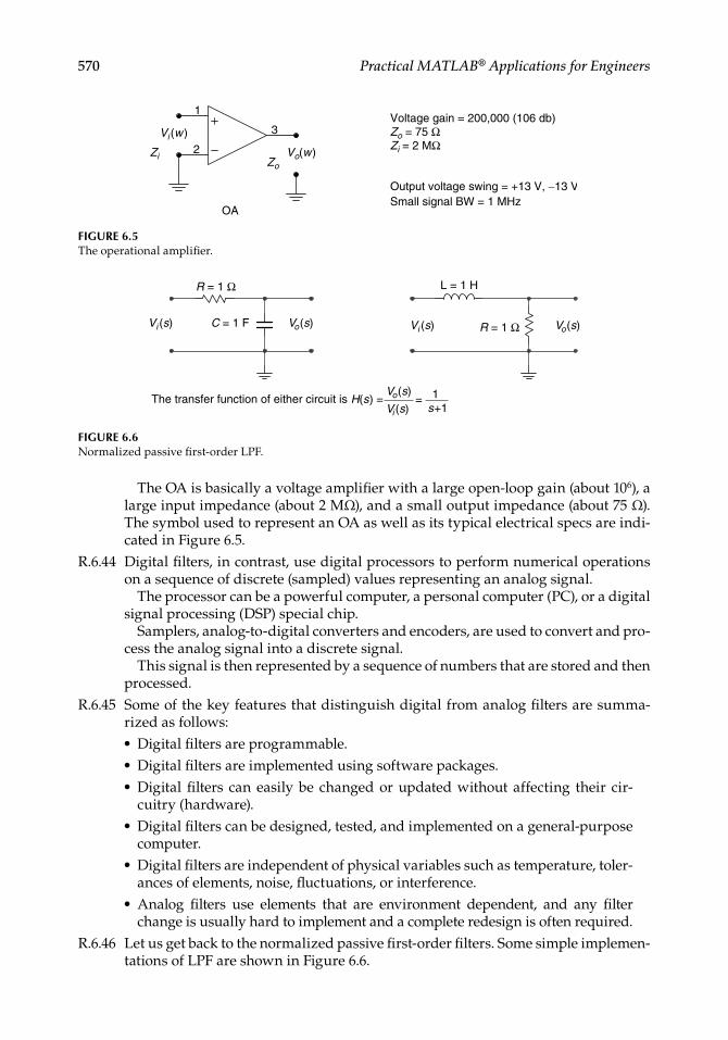
570 Practical MATLAB® Applications for Engineers
The OA is basically a voltage amplifi er with a large open-loop gain (about 106), a large input impedance (about 2 MΩ), and a small output impedance (about 75 Ω). The symbol used to represent an OA as well as its typical electrical specs are indi-cated in Figure 6.5.
R.6.44 Digital fi lters, in contrast, use digital processors to perform numerical operations on a sequence of discrete (sampled) values representing an analog signal.
The processor can be a powerful computer, a personal computer (PC), or a digital signal processing (DSP) special chip.
Samplers, analog-to-digital converters and encoders, are used to convert and pro-cess the analog signal into a discrete signal.
This signal is then represented by a sequence of numbers that are stored and then processed.
R.6.45 Some of the key features that distinguish digital from analog fi lters are summa-rized as follows:
Digital fi lters are programmable. Digital fi lters are implemented using software packages.Digital fi lters can easily be changed or updated without affecting their cir-cuitry (hardware).Digital fi lters can be designed, tested, and implemented on a general-purpose computer.Digital fi lters are independent of physical variables such as temperature, toler-ances of elements, noise, fl uctuations, or interference. Analog fi lters use elements that are environment dependent, and any fi lter change is usually hard to implement and a complete redesign is often required.
R.6.46 Let us get back to the normalized passive fi rst-order fi lters. Some simple implemen-tations of LPF are shown in Figure 6.6.
•••
•
•
•
FIGURE 6.5The operational amplifi er.
1
2
3Vi (w )
Vo(w)Zo
Zi
OA
Voltage gain = 200,000 (106 db)Zo = 75 ΩZi = 2 MΩ
Output voltage swing = +13 V, −13 VSmall signal BW = 1 MHz
FIGURE 6.6Normalized passive fi rst-order LPF.
R = 1 Ω
R = 1 ΩC = 1 F
L = 1 H
Vi (s) Vi (s)Vo(s) Vo(s)
H(s) = Vo(s)
Vi (s)= 1
s+1The transfer function of either circuit is
CRC_47760_CH006.indd 570CRC_47760_CH006.indd 570 7/23/2008 2:26:32 PM7/23/2008 2:26:32 PM

Analog and Digital Filters 571
Observe that the effect of the inductor in an LPF can be replaced by a capacitor. R.6.47 Examples of normalized passive fi rst-order HPFs are illustrated in Figure 6.7.
Observe again that the effect of the inductor in the HPF can be replaced by employ-ing a capacitor.
R.6.48 The preceding simple prototype fi lter types (LP and HP) are typically implemented as segments (eliminating the resistors), and are referred to as T and π sections, dis-cussed in R.6.49.
R.6.49 Typical T and π LPF prototype segments, also referred to as sections or blocks, are illustrated in Figure 6.8.
An all-pole prototype LPF can be realized by connecting T sections as illustrated in Figure 6.9. The order of the fi lter is then given by the total number of indepen-dent capacitors and inductors. For the network shown in Figure 6.9, the order n of the LPF is given by n = 2m.
R.6.50 Typical HP T and π sections are illustrated in Figure 6.10, and are obtained by replacing the inductors by capacitors and capacitors by inductors of the LP sections shown in Figure 6.8.
FIGURE 6.7Normalized passive fi rst-order HPF.
R = 1 Ω
R = 1 ΩC = 1 F
L = 1 HVi (s) Vi (s)Vo(s) Vo(s)
H(s) = Vo(s)
Vi (s)= s
s+1The transfer function of either network is given by
FIGURE 6.8T and π LPF prototype segments.
L /2 L /2 L
C C C
FIGURE 6.9All-pole prototype LPF.
L1 L2 Lm − 1 LmC1 C 2 Cm − 1 Cm R
FIGURE 6.10T and π HPF prototype segments.
C CL
CL L
CRC_47760_CH006.indd 571CRC_47760_CH006.indd 571 7/23/2008 2:26:32 PM7/23/2008 2:26:32 PM

572 Practical MATLAB® Applications for Engineers
FIGURE 6.11Typical active fi lter structures and its respective transfer functions.
R1
R1
R2
R2
R1
R1
R 2
R 2
C 2
C 1
C 1
C 2
C 2
C 1
1
23
Vi
Vi
Vi
Vi
Vo
Vo
Vo
Vo
1
2
3
a1 =
Hlp (s )=
Hhp (s ) =
1
23
1
23
Hbr (s) =
Hbp (s) =
A =
(R1*C1) (R2*C2)a2 =
1 1
1
,
A s + a2
R1*C 21
R2R1 s + a1
s
s + a1
s + a2C2C 1
(s + a2)(s + a1)A
R.6.51 Let us turn our attention to the most common active fi lter structures. Confi gura-tions as well as the respective transfer functions are indicated in Figure 6.11.
R.6.52 The loading effects associated with passive fi lters are overcome by using OA. Many complex fi lter realizations can then be implemented by connecting prototypes result-ing into products or sum structures of simple (fi rst- or second-order) fi lter types.
R.6.53 Figure 6.12 illustrates a second-order BRF employing simple fi rst-order fi lters (LP and HP, with w2 > w1). Observe that by changing the summation by a product (by cascading an LP with an HP, with w1 > w2), a BPF may be implemented.
CRC_47760_CH006.indd 572CRC_47760_CH006.indd 572 7/23/2008 2:26:33 PM7/23/2008 2:26:33 PM

Analog and Digital Filters 573
R.6.54 Practical fi lters often used in applications (appliances) are named after the research-ers, often mathematicians who studied the polynomials that make up the transfer function that best matches the ideal fi lter characteristics.
The most common practical fi lters are referred to asa. Butterworthb. Chebyshevc. Cauer (elliptic) d. Bessel
These fi lters return characteristics based on the facts that the system transfer function presents regions with smooth or ripple (oscillations) behavior.
R.6.55 The Butterworth fi lter is probably the most popular practical fi lter. The fi lter char-acteristics consist of maximum fl at response in the pass-band region, with no rip-ples either in the pass band or stop band.
The basic design approach consists of choosing an appropriate model of the transfer function H(jw). From this transfer function, the complex conjugate H(−jw) is then obtained, and from the product H(jw) * H(−jw) = H(jw)2 the poles of the transfer function can be evaluated.
The Butterworth magnitude-squared response of an n-order LPF is given by the following equation:
H(jw) * H( jw) H (jw)a
2 1
1
2wwp
n
(The subindex a in H stands for analog.)The normalized Butterworth magnitude is given by
FIGURE 6.12Second-order BRF employing simple fi rst-order LP and HP fi lters.
HLP(w)
HHP(w)
HBR(w )
Vi
Vo
w1
w2w
w
∑
CRC_47760_CH006.indd 573CRC_47760_CH006.indd 573 7/23/2008 2:26:33 PM7/23/2008 2:26:33 PM

574 Practical MATLAB® Applications for Engineers
H (jw)a
1
1
2 1 2
wwp
n
/
Table 6.3 provides the transfer function H(jw) for the case of LP normalized fi lters of the order n = 1, 2, 3, 4, and 5.
The denominators of H(jw) are commonly referred to as the Butterworth polyno-mial of order n. Figure 6.13 illustrates the magnitude response of the normalized Butterworth LPFs for the following orders n = 1, 2, 3, 4 and 10.
Observe that as the order increases (n), the pass-band region becomes fl atter and the transition region narrows.
Observe also that the maximum fl atness occurs at low frequencies (the limiting case is w = 0).
TABLE 6.3
Butterworth Polynomials
n H(jw)
1 [jw + 1]−1
2 [( jw)2 + 1.41( jw) + 1]−1
3 [( jw)3 + 2( jw)2 + 2( jw) + 1]−1
4 [( jw)4 + 2.613( jw)3 + 3.414( jw)2 + 2.613( jw) + 1]−1
5 [( jw)5 + 3.236( jw)4 + 5.236( jw)3 + 5.2361( jw)2 + 3.2361( jw) + 1]−1
FIGURE 6.13Magnitude plots of normalized Butterworth LPFs of orders n = 1, 2, 3, 4, and 10.
0 1 2 3 4 5 6
0
0.1
0.2
0.3
0.4
0.5
0.6
0.7
0.8
0.9
1
Normalized frequency
Gai
n
Butterworth LPF/order n = 1, 2, 3, 4, 10
n = 3
n = 1
n = 10
n = 4
n = 2
CRC_47760_CH006.indd 574CRC_47760_CH006.indd 574 7/23/2008 2:26:33 PM7/23/2008 2:26:33 PM

Analog and Digital Filters 575
R.6.56 Observe also that the two parameters that completely specify the Butterworth fi lter are
The 3 dB cutoff frequency wp
The order nThe Butterworth fi lter uses the Taylor series approximation to model the ideal
LPF prototypes for the two key frequencies: w = 0 and w = ∞ (for any order n).R.6.57 Analog-Chebyshev fi lters trade off fl atness in the pass band for a shorter transi-
tion band. The main objective of this fi lter is to minimize the design error, where the error is defi ned as the difference between the ideal LPF (brick wall) fi lter and the implementation of the actual response of the fi lter over a prescribed band of frequencies.
The magnitude is either given by an equiripple gain in the pass band and a monotic behavior in the stop band or a monotonic behavior in the pass band and equiripple in the stop band, depending on the fi lter type.
Chebyshev fi lters are classifi ed according to their ripple and monotonicity asType 1Type 2
R.6.58 The type-1 Chebyshev transfer function minimizes the difference between the ideal (brick wall) and the actual frequency response over the entire pass band by returning equal magnitude ripple in the pass band and a smooth decrease with maximum fl atness gain in the stop band (see Figure 6.14).
R.6.59 The type-2 Chebyshev fi lter transfer function, also referred to as the inverse Cheby-shev transfer function fi lter minimizes the difference between the ideal (brick wall) and the actual frequency response over the entire stop band by returning an equal
••
••
FIGURE 6.14(See color insert following page 374.) Magnitude plots of normalized analog Chebyshev type-1 LPFs of orders n = 1, 2, 3, 4, and 10.
0 0.5 1 1.5 2 2.5 3 3.5 40
0.2
0.4
0.6
0.8
1
Normalized frequency
Gai
n
Chebyshev type-1 LPF/order n = 1, 2, 3, 4, 10
n = 1
n = 3n = 4n = 10
n = 2
CRC_47760_CH006.indd 575CRC_47760_CH006.indd 575 7/23/2008 2:26:34 PM7/23/2008 2:26:34 PM

576 Practical MATLAB® Applications for Engineers
ripple in the stop band and a smooth gain with maximum fl atness in the pass band (see Figure 6.15).
The stop band does not approach zero as fast as type 1. The ripple effect becomes more evident as the order of the fi lter increases.R.6.60 The magnitude square of the transfer function H(jw) of a Chebyshev type-1 fi lter is
given by
H w
C w wan p
( )( )
2
2 2
11
where Cn(x) is referred to as the Chebyshev polynomial of order n, in the region defi ned by
1
11
2
2 0 5 H w w wa p( )
( ) .
for
where ε denotes the maximum stop band deviation.The Chebyshev polynomial coeffi cients Cn(x) of order n are defi ned by
C x
n x x
n x xn( )cos( cos ( ))cos( cosh ( ))
1
1
0 11
forfor
FIGURE 6.15(See color insert following page 374.) Magnitude plots of normalized analog Chebyshev type-2 LPFs of orders n = 1, 2, 3, 4, and 10.
0 1 2 3 4 5 6
0
0.2
0.4
0.6
0.8
1
Normalized frequency
Gai
nChebyshev type-2 LPF/order n = 1, 2, 3, 4, 10
n = 1
n = 3
n = 4n = 2
n = 10
CRC_47760_CH006.indd 576CRC_47760_CH006.indd 576 7/23/2008 2:26:34 PM7/23/2008 2:26:34 PM

Analog and Digital Filters 577
The Chebyshev polynomial coeffi cients Cn(x) oscillate between –1 and 1, and can be generated by using the recursion equation given as follows:
Cn+1(x) = 2Cn(x) − Cn−1(x)
with C0(x) = 1 and C1(x) = x.Table 6.4 shows the Chebyshev polynomials for n = 1, 2, 3, and 4.Figure 6.14 displays the magnitude responses of an analog Chebyshev type-1 LPF
for n = 1, 2, 3, 4, and 10.
R.6.61 The Chebyshev type-2 fi lter is the complement of the Chebyshev type-1 fi lter, in the sense that the magnitude response is smooth in the pass band and presents equal ripple in the stop band.
Unlike the type-1 fi lter, which consists only of poles, the type-2 fi lters consist of both poles and zeros.
The magnitude square of the response is given by
H jwC w w
C w w
C w w
an s
n s p
n s
( )( )( )
( )
2 2
2
2
1
where ∈ defi nes the maximum stop-band deviation, wp denotes the pass-band cutoff frequency, ws denotes the stop-band cutoff frequency, and Cn(x) are the Chebyshev polynomials (defi ned in Table 6.4).
Figure 6.15 shows the magnitude responses of an analog Chebyshev type-2 fi lters for n = 1, 2, 3, 4, and 10.
R.6.62 Elliptic fi lters, also known as Cauer fi lters, present ripples in the pass as well as in the stop-band regions. The main characteristic of the elliptic fi lter is that the transi-tion band is the narrowest with respect to the other two fi lter types, the Butterworth and Chebyshev fi lters.
The square of the magnitude of the transfer function of the Cauer fi lters is given by
H jw
J w han
( )( , )
2
2 21
1
where ε is the pass-band deviation, Jn(w, h) is the n-order Jacobian, and h indicates the ripple’s height (in the pass- and stop-band regions).
Figure 6.16 shows the magnitude response of an elliptic fi lter for n = 1, 2, 3, 4, and 10.
R.6.63 Butterworth, Chebyshev (types 1 and 2), and elliptic fi lters deal basically with the magnitude response, with little concern about their phase response.
TABLE 6.4
Chebyshev Polynomials
n Cn(w)
1 w2 2w2 − 13 4w3 − 3w4 8w4 − 8w2 + 1
CRC_47760_CH006.indd 577CRC_47760_CH006.indd 577 7/23/2008 2:26:34 PM7/23/2008 2:26:34 PM

578 Practical MATLAB® Applications for Engineers
R.6.64 Bessel fi lters, also known as linear-phase fi lters, present a linear-phase response in the pass band, in addition they try to approximate the magnitude response in the pass-band region satisfying the desired specs.
The system transfer function of an nth-order Bessel fi lter is given by the transfer function shown as follows:
H jw
nn B jwa n
n
( )( )!! ( )
2
2
where Bn(jw) is the n-order Bessel polynomial defi ned by
B jw
n jwl nn
l
nl
n
( )( )!( )
!( )!
2 12 11
0∑
Figure 6.17 shows the magnitude response and Figure 6.18 shows the phase response of the Bessel fi lters for orders n = 1, 2, 3, 4, and 10.
R.6.65 It is obvious that the mathematics involved in either the analysis or synthesis of any type of fi lter is generally a complicated and complex proposition, which is dif-fi cult and labor intensive. This book attempts to defi ne the fi lter types often used in real application and provides an overview of the fi lter theory and a simple and user friendly approach to the analysis and synthesis process. The mathematical complexities of the power of fi lter theory, in either the synthesis or analysis pro-cesses, can be avoided by using MATLAB.
FIGURE 6.16(See color insert following page 374.) Magnitude plots of normalized analog elliptic LPFs of orders n = 1, 2, 3, 4, and 10.
0 1 2 3 4 5 60
0.2
0.4
0.6
0.8
1
Normalized frequency
Gai
n
Elliptic LPF/order n = 1, 2, 3, 4, 10
n = 1
n = 4, 10
n = 2
n = 3
CRC_47760_CH006.indd 578CRC_47760_CH006.indd 578 7/23/2008 2:26:35 PM7/23/2008 2:26:35 PM

Analog and Digital Filters 579
FIGURE 6.17(See color insert following page 374.) Magnitude plots of normalized analog Bessel LPFs of orders n = 1, 2, 3, 4, and 10.
0 2 4 60
0.2
0.4
0.6
0.8
1
n = 1
n = 3n = 10
n = 4
Bessel magnitude LPF/order n = 1 , 2, 3, 4, 10
Normalized frequency
Gai
n
n = 2
FIGURE 6.18(See color insert following page 374.) Phase plots of normalized analog Bessel LPFs of orders n = 1, 2, 3, 4, and 10.
0 0.5 1
−3
−2
−1
0
1
2
3
Normalized frequency
Pha
se in
rad
ian
Bessel phase LPF/order n = 1, 2, 3, 4, 10
n = 3
n = 2
n = 1
n = 10
n = 4
CRC_47760_CH006.indd 579CRC_47760_CH006.indd 579 7/23/2008 2:26:35 PM7/23/2008 2:26:35 PM

580 Practical MATLAB® Applications for Engineers
MATLAB offers a number of functions that can be used in the analysis and syn-thesis of almost any fi lter type. The corresponding MATLAB function fi les are pre-sented and discussed in R.6.66 through R.6.72.
R.6.66 The following function fi les can be used in the analysis and synthesis of analog Butterworth fi lters:a. [z, p, k] = buttap(n) returns the zeros (z), poles (p), and gain factor (k) of the normal-
ized analog Butterworth LPF transfer function of order n (with a cutoff frequency given by wp = 1 rad/s).
b. [num, den] = butter(n, wn, ‘s’) returns the numerator and denominator polynomial coeffi cients as row vectors in descending powers of s, of an n-order transfer func-tion of an LPF with a cutoff frequency at wn rad/s. If wn consists of a two-element vector [wl, wu], where wl < wu, the function returns a second-order band-pass transfer function with drops at the wl and wu edges, and a BW given by wu − wl.
c. [num, den] = butter(n, wn, ‘fi ltertype’, ‘s’) returns an n-order HP or band-stop (BS) fi lter of order 2n, where ‘fi ltertype’ is specifi ed as ‘high’ for an HPF, or ‘stop’ for a BSF with the (3 dB) stop-band edges given by wn = [wl, wu], where wl < wu.
d. [n, wn] = buttord(wp, ws, Rp, Rs, ‘s’) returns the lowest-order Butterworth fi lter (n) given by the fi lter parameters defi ned bywp = Pass-band edge (rad/s) ws = Stop-band edge (rad/s)Rp = Maximum pass-band attenuation (dB)Rs = Minimum stop-band attenuation (dB)n = Order of the fi lterwn = Cutoff frequency (rad/s)
R.6.67 The MATLAB function [num, den] = maxfl at (a, b, wp ) returns a Butterworth-type fi lter with the transfer function having two orders given by a and b, where a defi nes the degree of the num (numerator) and b the den (denominator) of the fi lter’s transfer function instead of just using one order, and where wp is the pass-band edge that takes a value over the range 0–1.
When the orders of the num and den are the same (a = b), the functions maxfl at and butter return the same fi lter results.
R.6.68 For example, verify that the maxfl at and butter MATLAB functions return the same fi lter specs for the case when a = b = 4 and wp = 0.3.
MATLAB Solution>> [num,den] = maxflat (4,4,0.3)
num = 0.0186 0.0743 0.1114 0.0743 0.0186 den = 1.0000 -1.5704 1.2756 -0.4844 0.0762
>> [num,den] = butter(4,0.3)
num = 0.0186 0.0743 0.1114 0.0743 0.0186 den = 1.0000 -1.5704 1.2756 -0.4844 0.0762
CRC_47760_CH006.indd 580CRC_47760_CH006.indd 580 7/23/2008 2:26:35 PM7/23/2008 2:26:35 PM

Analog and Digital Filters 581
R.6.69 The following example illustrates the case where the desired transfer function of an LP Butterworth fi lter is given by a denominator polynomial of order 6, whereas the numerator polynomial is of order 4, and wp = 0.3.
MATLAB Solution>> [num,den] = maxflat (4,6,0.3)
num = 0.0086 0.0344 0.0515 0.0344 0.0086 den = 1.0000 -2.4633 3.0480 -2.1861 0.9427 -0.2278 0.0239
R.6.70 Once the poles, zeros, and gain of the desired fi lter transfer function are known (indi-cated by the variables p, z, and k), the numerator and denominator polynomial coef-fi cients of the transfer function can be obtained by using the MATLAB function
[num, den] zp2tf(z, p,k)
R.6.71 The following function fi les can be used in the analysis and synthesis of analog Chebyshev type-1 fi lters:a. [z, p, k] = cheblap(n, Rp ) returns the zeros (z), poles (p), and gain factor (k) of the
normalized analog type-1 Chebyshev LPF transfer function of order n with a pass-band ripple Rp expressed in decibels.
b. [num, den] = cheby1(n, Rp, wn, ‘s’) returns the num and den of the LPF transfer function of order n (numerator and denominator) as vectors consisting of the polynomial coeffi cients of the transfer function in descending powers of s, given Rp (pass-band ripple in decibel) and wn (pass-band edge in radians/second).
If wn is specifi ed as a two-element vector such as wn = [wl, wu], where wl < wu, the function returns the transfer function of a second-order BPF with pass-band edges given by wl and wu.
c. [num, den] = cheb1(n, Rp, wn, ‘fi ltertype’, ‘s’) returns the num and den of the transfer function of order n (numerator and denominator) as vectors consisting of the polynomial coeffi cients arranged in descending powers of s. When ‘fi ltertype’ is specifi ed as ‘high’ for an HPF, or ‘stop’ for a BSF, then wn = [wu, wl] is given by two values, for wu > wl, given the band-pass ripple Rp (in decibels).
d. [n, wn] = cheb1ord(wp, ws, Rp, Rs, ‘s’) returns the lowest LPF order (n) of the Chebyshev type-1 analog fi lter, where wn indicates the cutoff frequency (radians per second), given the following input variables:wp = Pass-band edge (rad/s) ws = Stop-band edge (rad/s)Rp = Maximum pass-band attenuation (dB)Rs = Minimum stop-band attenuation (dB)
R.6.72 The function fi les used for the analysis and synthesis of analog type-2 Chebyshev fi lters are summarized as follows:a. [z, p, k] = cheb2ap (n, Rs)
b. [num, den] = cheby2 (n, Rs, wn, ‘s’)
c. [num, den] = cheby2 (n, Rs, ‘fi ltertype’, ‘s’)
d. [n, wn] = cheb2ord (wp, ws, Rp, Rs, ‘s’)
CRC_47760_CH006.indd 581CRC_47760_CH006.indd 581 7/23/2008 2:26:36 PM7/23/2008 2:26:36 PM

582 Practical MATLAB® Applications for Engineers
The variables used in the preceding function fi les are defi ned as follows:z = Zeros of the transfer functionp = Poles of the transfer functionk = Gain of the transfer functionnum = Numerator coeffi cients of the transfer function given as vectors in descend-
ing powers of sden = Denominator coeffi cients of the transfer function given as vectors in descend-
ing powers of sn = Order of fi lterRs = Minimum stop-band ripple attenuation (dB)wn = Pass-band edge (rad/s)Rp = Maximum pass-band ripple attenuation (dB)wp = Pass-band edge (rad/s)‘fi ltertype’ = High or stop (for either HP or BP)
The type-2 Chebyshev fi lter functions are self-explanatory since they are similar in syntax and content to the function defi ned in R.6.71 for the Chebyshev type-1 fi lter.
R.6.73 The following function fi les can be used in the analysis and synthesis of the analog elliptic fi lters:a. [z, p, k] = elliap (n, Rs)b. [num, den] = ellip (n, Rs, wn, ‘s’)c. [num, den] = ellip (n, Rs, ‘fi ltertype’, ‘s’)d. [n, wn] = ellipord (wp, ws, Rp, Rs, ‘s’)
Note that the elliptic fi lter functions follow the syntax and content similar tothe function fi les defi ned for the Butterworth and Chebyshev fi lters, and no further function description is given. The workout examples provide insight of the specifi c function and applications.
R.6.74 The function fi les used in the analysis and synthesis of the Bessel fi lters are defi ned as follows:a. [z, p, k] = besselap (n)b. [num, den] = besself (n, wn)c. [num, den] = besself (n, wn, ‘fi ltertype’)
The functions and variables used in the Bessel functions are self-explanatory and in case of doubt refer to the Chebyshev and elliptic fi lter function descriptions (R.6.71).
R.6.75 In most fi lter problems, the MATLAB functions that return the zeros, poles, and gain forms provide a more accurate response than the ones using the transfer function.
For fi lters of order 15 or less, the function fi les that return the num (numerator) and den (denominator) of the transfer function can safely be used, but for fi lters of orders greater than 15, the zeros, poles, and gain returns a more reliable version.
R.6.76 Some important observations of the different fi lter’s phase prototypes are summa-rized as follows: a. Butterworth and Chebyshev fi lters present a linear-phase response over a good
portion of the pass-band region.b. Bessel fi lters are generally used when the desired phase response is linear over
a larger portion of the pass band.
CRC_47760_CH006.indd 582CRC_47760_CH006.indd 582 7/23/2008 2:26:36 PM7/23/2008 2:26:36 PM

Analog and Digital Filters 583
R.6.77 The MATLAB function [numL, demL] = lp2lp (numN, denN, wc) is used to transform a normalized LPF prototype given by the transfer function H(s) = numN(s)/denN(s) into a denormalized LPF with a numerator numL, denominator denL, and cutoff fre-quency wc. This function fi le returns the coeffi cients of the polynomials numL and denL as a row vector arranged in descending powers of s.
R.6.78 Similarly, the MATLAB function [numH, denH] = lp2hp (numN, denN, wc) is used to transform a low-pass normalized fi lter into a denormalized HPF with the pass band given by wc.
R.6.79 The function fi le [numbp, denbp] = lp2bp (numN, denN, wo, BW) transforms an LP nor-malized fi lter into a BPF or BSF (lp2bs), where wo is its center frequency with BW.
R.6.80 Some practical observations of the resulting fi lter complexity and their associated costs are summarized as follows:
a. The complexity of a fi lter is generally given by its order n. The higher the order, the greater the complexity and cost in term of elements.
b. Generally, for a particular set of fi lter specs, the elliptic fi lter implementation is less complex than the equivalent Chebyshev (type 1 or 2).
c. The Chebyshev (type 1 or 2) cost is considerably less than its Butterworth equiv-alent counterpart.
d. An estimate of the fi lter complexity is given by the following example: an elliptic fi lter of order 6 requires an equivalent Chebyshev fi lter (type 1 or 2) of order 10 and a Butterworth equivalent implementation of order 29.
R.6.81 Recall that digital fi lters as well as analog fi lters have as their primary objective to fi lter, meaning to pass or reject, certain band of frequencies. Analog fi lters are expressed as functions of w (radians per second), whereas digital fi lters are func-tions of W = w * T called the scaled or digital frequency, where T is the sampling period (sometimes indicated by Ts).
R.6.82 Recall that by using the digital frequency W (some textbooks use Ω), the frequency response of the digital fi lter is always periodic with period 2π.
R.6.83 Digital fi lters can be classifi ed based on their impulse response length as follows:
a. FIR b. IIR
R.6.84 An FIR fi lter returns an impulse response with an amplitude that decays to zero in a fi nite number of steps (samples) or duration.
R.6.85 An IIR fi lter returns an impulse response that has, in theory, an infi nite duration or continues forever because of its recursive nature (feedback).
This defi nition is not accurate because the impulse response of any system including IIR fi lters in real life eventually decay to zero in a fi nite time, which may be long.
R.6.86 IIR fi lters are used to closely approximate the gain and phase response of analog fi lters and the specs are usually given in terms of analog variables such as BW, minimum pass-band ripple (Rp ), and maximum stop-band ripple (Rs). These types of fi lters can substitute analog fi lters.
R.6.87 The approach followed in the design of IIR fi lters are as follows:a. Design an analog prototype with the desired frequency response (transfer func-
tion) given by its transfer function H(s).
CRC_47760_CH006.indd 583CRC_47760_CH006.indd 583 7/23/2008 2:26:36 PM7/23/2008 2:26:36 PM

584 Practical MATLAB® Applications for Engineers
b. Transform the analog fi lter into its digital version by obtaining the discrete fi lter transfer function H(z) or its impulse response h(n).
R.6.88 One fundamental difference exists between H(s) and its discrete mapping H(z). Since the phase function of the digital prototype is given by
∠H(z) = tan−1 [Imag(H(z)/Real(H(z)] + /2(1 + sign(Real(H(z)))
where z = jW.Then the gain presents a periodic behavior (with period 2π), then the principal
value is limited over the digital frequencies over the range −π ≤ W ≤ +π.R.6.89 The steps involved in the design of IIR fi lters using MATLAB are summarized as
follows:1. Design an analog LP normalized prototype fi lter2. Use frequency transformation to transform the LP analog prototype into the
desired fi lter type: LP, HP, BP, or BS fi lter depending on the requirements of the design (using the MATLAB functions: lp2lp, lp2hp, etc.)
3. Transform the analog fi lter into its digital version bya. Bilinear transformationb. Impulse invariant method c. Yule–Walker algorithm
These techniques are presented and discussed in the following.R.6.90 The bilinear transformation is a one-to-one mapping of the complex analog fre-
quency s(s = σ + jw) of the transfer function H(s) (s-plane) into the complex digital frequency z(z = esT) (z-plane).
R.6.91 Mathematically, the mapping s (analog) → z (digital) or z → s is accomplished by the following substitution:
s → A
zz
12
or
z → A s
A s
where A = 2/T, in which T is the sampling period.The objective of the mapping is to move the poles and zeros of the desired analog
transfer function H(s) from the s-plane into the z-plane.R.6.92 The effect of the bilinear transformation results in moving the poles and zeros from
the left half of the s-plane into the unit circle in the z-plane, where the imaginary axis in the s-plane is mapped into the outside of the unit circle of the z-plane and the right half of the s-plane is mapped into the outside of the unit circle of the z-plane guaranteeing stability in this way.
Therefore, a stable analog fi lter H(s) results in a stable digital fi lter H(z).Recall that to analyze the stability of a digital fi lter it is suffi cient to compute the
magnitude of the poles, and if they are smaller in magnitude than 1 (inside the unit circle), then the system is stable otherwise the system is unstable.
R.6.93 Since the analog frequency w (radians per second) is related to the digital frequency W (radians) by the relation W = wT, the infi nite range of w(−∞ to +∞) in the s-plane is compressed into the range −π ≤ W ≤ π (referred to as frequency wrapping).
CRC_47760_CH006.indd 584CRC_47760_CH006.indd 584 7/23/2008 2:26:36 PM7/23/2008 2:26:36 PM

Analog and Digital Filters 585
R.6.94 The resulting relation between the analog frequency w and the discrete frequency W is given by
W (2 T) tan(W/2) * (a nonlinear frequency transformation)
or
W 2 arctan(w T/2) * *
R.6.95 The MATLAB function unwrap(phase) unwraps the phase angle (in radians) and lim-its the phase over the range of interest given by −π ≤ W ≤ +π.
R.6.96 The other transformations used in the design of LP, HP, BP, or BS fi lters from the analog prototypes into the digital ones are given as follows: a. LP: s = (2/T) * [(z − 1)/(z + 1)], w = (2/T) * tan(W/2)b. HP: s = (2/T) * [(z + 1)/(z − 1)], w = −(2/T) * cot(W/2)c. BP: s = (2/T) * [(z2 − 2 * c * z + 1)/(z2 − 1)], w = (2/T) * [(c − cos(W))/(sin(W))]d. BS: s = (2/T) * [(z2 − 1)/(z2 − 2 * c * z + 1)], w = (2/T) * [(c − cos(W))/(sin(W))]−1
R.6.97 An example of a bilinear transformation is provided as follows: Let us transform the fi rst-order analog (RC) LPF illustrated by the circuit diagram of Figure 6.6 into a digital fi lter. Recall that the fi lter transfer function is given by
H wV jwV jw
jwC
jwCR
R C
j wR C
o
i
( )( )( )
*
**
1
1
1
1
without any loss of generality let R = C = 1 and s = jw, then
H s
V sV s s
o
i
( )( )( )
11
Assuming that the sampling period is T = 2 and applying the corresponding bilinear transformation defi ned in R.6.96 yields
H szz z
z
11
111
1
then the discrete transform becomes
H(z) z 0.5 0.5 * 1
Note that in this simple example the resulting digital fi lter is an FIR. A more complex analog fi lter transformation could result in an IIR fi lter. Hand computa-tions can be avoided by using MATLAB as indicated in R.6.98.
R.6.98 The MATLAB function [numz, denz] = bilinear (numa, dena, 1/Ts ) returns the dis-crete polynomial coeffi cients numz and denz (numerator and denominator of H(z)) arranged in descending powers of z, where numa and dena are the analog numera-tor and denominator of H(s), where Ts indicates its sampling rate.
CRC_47760_CH006.indd 585CRC_47760_CH006.indd 585 7/23/2008 2:26:37 PM7/23/2008 2:26:37 PM

586 Practical MATLAB® Applications for Engineers
R.6.99 The function [pz, zz, kz] = bilinear (pa, za, ka, fs, fc) returns the digital poles, zeros, and gain given by pz, zz, and kz of its discrete transfer function H(z), where pa, za, and ka are the analog poles, zeros, and gain of H(s), where fs = 1/Ts and fc = 1/(2π).
The bilinear transformation with the optional frequency prewarping is given by [pz, zz, kz] = bilinear (pa, za, ka, fs) returns the s-domain analog transfer function specifi ed by pa, za, ka, fs into the z discrete equivalent transfer function given by the following substitutions:
H z H s
s fszz
( ) ( ) ( )( )
2
11
∗
where the column vectors za and pa are the analog zeros and poles of H(s), and fs represents its sample frequency in hertz.
R.6.100 The impulse invariant response method converts the impulse response of the desired analog fi lter h(t) into an equivalent digital FIR h(n), by properly sampling h(t), with the hope that the analog response would closely follow its digital response. Hence, the digital fi lter preserves the impulse response of the original analog fi lter.
R.6.101 Observe that the bilinear transformation is a process done entirely in the frequency domain, whereas the impulse response method is done in the time domain.
R.6.102 The impulse invariant IIR fi lter is realized by the following steps:a. h(t) = £−1 [H(s)]
b. Substitute t by nT
c. Obtain the digital transfer function H(z) = Z[h(nT)] * TObserve that the analog fi lter impulse response would then have the same val-
ues as the sample digital fi lter impulse response at the sampling instances nT.Recall that when the inverse Laplace transform of H(s) cannot be obtained
directly, then a partial fraction expansion of H(s) may be required for obtaining in this way a parallel structure implementation.
R.6.103 The impulse invariant method suffers from aliasing, and this is the main reason that it is not widely used. The bilinear transformation does not suffer from alias-ing and is by far more popular than the impulse invariance method.
R.6.104 The step invariant technique is an alternate way in the implementation of an IIR fi lter by working with the step response instead of the impulse response. The step response of the analog fi lter would then have the same values at the sampling instances as the digital fi lter step response.
R.6.105 Mathematically, the impulse invariance response transforms H(s) into H(z) [H(s) → H(z)] by making the following substitution:
1 11 1s a z e aT
⇒
(transformation used for simple poles of H(s)).
s as as a b
z e bTz e bT z e
aT
aT aT
2 2 2
1
1 2 221
1 2⇒ cos( )
cos( )
bs as a b
z e bTz e bT z e
aT
aT aT2 2 2
1
1 2 221
1 2
⇒ sin( )
cos( )
CRC_47760_CH006.indd 586CRC_47760_CH006.indd 586 7/23/2008 2:26:37 PM7/23/2008 2:26:37 PM

Analog and Digital Filters 587
(transformations used for the case of complex poles of H(s)).R.6.106 For example, let the analog transfer function of a second-order Butterworth low
pass-band fi lter be given by
H s
s s( )
.
10014 14 1002
Use the impulse invariant method to transform the analog fi lter into a digital one if the sampling rate is given by T = 0.0314 s.
ANALYTICAL Solution
Rearranging the terms of H(s) into the format given in R.6.105 results in
H s
s s( )
( . ) ( . ) ( . )
1002 14 14 2 14 14 2 100 14 14 22 2 2
H s
s s( )
( . ) ( . ) ( . )
1002 14 14 2 7 07 100 7 072 2 2
H s
s s( ) *
( . ) ( ) ( )
2 502 14 14 2 50 100 502
H s
s s( ) * ( ) ( )
( . ) ( ) ( )
2 50 502 14 14 2 50 50
1 2 1 2
2
H s
s s( ) * ( )
( )( . ) ( . ) ( . )
2 5050
2 14 14 2 7 07 7 071 2
1 2
2 2 2
H s
s s( ) * ( )
.( . ) ( . ) ( . )
2 507 07
2 14 14 2 7 07 7 071 2
2 2 2
Then, let a = 7.07, b = 7.070, and T = 0.0314, and using the substitutions of R.6.105 H(s) → H(z) the following discrete system is obtained: The numerator of [H(z)] = [2 * (50)1/2]) * [z–1e−(7.07)*(0.0314) * sin(7.07 * 0.0314)] and the denominator of [H(z)] = [1 − 2z−1e−(7.07)*(0.0314) * cos(7.07 * 0.0314) + z−2e−2 * 7.07 * 0.0314].
Then, after performing the corresponding algebraic manipulations the follow-ing simplifi ed expression is obtained:
H z
Y zX z
zz z
( )( )( )
.. .
2 50
0 08821 1 5626 0 6414
1
1 2*
As a consequence of the sampling process (Nyquist theorem), the fi lter mag-nitude is multiplied by 1/T. Therefore, after the transformation process from the
CRC_47760_CH006.indd 587CRC_47760_CH006.indd 587 7/23/2008 2:26:37 PM7/23/2008 2:26:37 PM

588 Practical MATLAB® Applications for Engineers
continuous to the discrete domain is done, the fi lter transfer function has to be compensated by multiplying the response by T.
For this example, the fi nal transfer function would then be the preceding expres-sion for H(z) multiplied by T = 0.0314.
The reader can appreciate that the substitution and algebraic manipulations involved in the transformation process just presented is labor-intensive.
This computational effort can be avoided by using the power of MATLAB as illustrated in the following points.
R.6.107 The MATLAB function [numz, denz] = impinvar (nums, dens, fs) maps the analog transfer function H(s) into the discrete transfer function H(z) using the substitu-tions presented in R.6.105 and returns the numerator and denominator of H(z) = numz/denz, given the numerator and denominator of H(s) = num(s)/den(s), with a sampling frequency given by fs. The function impinvar used without specifying fs takes the default value of fs = 1 Hz.
R.6.108 The MATLAB function [numz, denz] = yulewalk (n, f, mag) returns the numerator numz and denominator denz, where H(z) = numz(z)/denz(z) as the polynomial coef-fi cients that best fi t the points defi ned by the vectors f and mag, where n denotes the fi lter order. f is a normalized vector specifying the set of key frequencies start-ing at 0 and ending at 1 and mag is the corresponding vector with the desired magnitude at the frequencies defi ned by f.
R.6.109 Unlike the transform of the analog prototype method, the yulewalk algorithm is a direct method to design a digital fi lter based on specs in the discrete domain with no constrains imposed by the standard fi lter prototypes. The digital fi lter coeffi cients are evaluated by obtaining the inverse fft of the desired, ideal power spectrum and then by solving the modifi ed Yule–Walker equations.
R.6.110 The FIR equivalent of this function is the MATLAB command fi r2, which also returns a fi lter based on a linear piecewise magnitude approximation.
R.6.111 MATLAB’s signal processing toolbox includes a number of functions that can directly be used in the analysis and synthesis of IIR fi lters based on the bilinear transformation.
The bilinear transformation functions based on the standard prototype fi lters are listed as follows:a. [numz, denz] = butter(n, wn )
b. [z, p, k] = butter(n, wn )
c. [numz, denz] = cheby1(n, Rp, wn )
d. [z, p, k] = cheby1(n, Rp, wn )
e. [numz, denz] = cheby2(n, Rs, wn )
f. [z, p, k] = cheby2(n, Rs, wn )
g. [numz, denz] = ellip(n, Rp, Rs, wn )
h. [z, p, k] = ellip(n, Rp, Rs, wn )
where numz and denz denote the numerator and denominator coeffi cients of H(z), Rp and Rs denote the pass- and stop-band ripples, n is the order of the fi lter, wn is the pass-band edge; a number between 0 and 1, z denotes discrete zeros, p denotes discrete poles, and k is the gain factor of the discrete transfer function while the sampling frequency is assumed to be 2 Hz or a sampling rate of T = 0.5 s.
CRC_47760_CH006.indd 588CRC_47760_CH006.indd 588 7/23/2008 2:26:38 PM7/23/2008 2:26:38 PM

Analog and Digital Filters 589
R.6.112 Recall that an IIR fi lter can be defi ned in the time domain by a difference equation. For example, let the system differential equation be given by
y(n) − 0.02y(n − 1) + 0.009y(n − 2) = 0.1x(n) + 0.2x(n − 1) + 0.3x(n − 2)
where x represents the input sequence and y is its output sequence.Observe that the output sequence y(n) is a function of the input sequence x(n) as
well as the previous (delayed) output sequences. R.6.113 An FIR fi lter can be defi ned by a difference equation with a fi nite input sequence x.
For example, let the system differential equation be given by
y(n) = 0.036x(n) − 0.02x(n − 1) + x(n − 2)
Observe that the output sequence y(n) is a function of its input sequence x(n) (scaled and delayed).
R.6.114 Some practical IIR design considerations and observations are summarized as follows:a. There is a ripple problem to consider.b. There is no guarantee that the design leads to a stable implementation.c. There is a stability problem to consider.d. Differences may exist among the different types of IIR fi lters.e. When the magnitude response is the main concern IIR is generally a good
choice.f. IIR fi lters require 5–10 times less coeffi cients than the equivalent FIR
implementation.R.6.115 An FIR fi lter is a fi lter that has a fi nite response for n < N and a linear phase, where
N is the length of the fi lter response. Such fi lters generally require N constant multipliers, N − 1 two port input adders and N stages of delays resulting in shift register–type structure.
R.6.116 All FIR fi lters present linear phase and an impulse response with some sort of symmetry that satisfi es the general relation given by
h(n) = ±h(N − n)
This sequence (h(n)) presents an even symmetry sequence for the positive case and an odd symmetry for the negative case, assuming the sequence h(n) consists of real coeffi cients.
R.6.117 The symmetry condition for the impulse response is a necessary condition for the linear phase.
R.6.118 The symmetry condition depends on the length of h(n) and whether N is odd or even.
R.6.119 Four types of symmetry conditions for FIR fi lters with real coeffi cients andlengths N result. They are summarized as follows:a. Type 1. Symmetric impulse response with N = odd.b. Type 2. Symmetric impulse response with N = even.
c. Type 3. Asymmetric impulse response with N = odd.
d. Type 4. Asymmetric impulse response with N = even.
CRC_47760_CH006.indd 589CRC_47760_CH006.indd 589 7/23/2008 2:26:38 PM7/23/2008 2:26:38 PM

590 Practical MATLAB® Applications for Engineers
R.6.120 Type-1 FIR fi lter is defi ned by the following relation:
h(n) = h(N − n) for 0 ≤ n ≤ N − 1, with N = odd.
Then the amplitude response is given by
H (W) a (n)cos(W )n1 1
e jNW
n
N2
0
2
∑
where a1(0) = h(N/2) is the mid-point and a1(n) = 2h((N/2) − n) for 1 ≤ n ≤ N/2.Type-1 FIR fi lters can be used to design any fi lter type. The following sequence
illustrates a type-1 FIR fi lter:
h(n) (n) (n ) (n ) (n 3) ( 0.09 0.30 0.3593 2 0.30 0.09 1 nn ) 4
R.6.121 The type-2 FIR fi lter is defi ned by
h(n) = h(N − n) for 0 ≤ n ≤ N − 1, with N = even
then
H (W) a (n)cos W(n )2 2 1 2
e jNW
n
N2
0
1 2
[ ]( )
∑
where
a n h
Nn n N2( ) ( )
2
12
1 2 1 2
=for , , …
Since the response is defi ned for −π ≤ W ≤ π, then
H (W )2 0
Therefore, type-2 FIR fi lters cannot be used to implement an HP or a BP fi lter.The following sequence illustrates a type-2 FIR fi lter:
h(n) = −0.09δ(n) + 0.30δ(n − 1) + 0.3593δ(n − 2) + 0.3593δ(n − 3)
+ 0.30δ(n − 4) −0.09δ(n − 5)
R.6.122 The type-3 FIR fi lter is defi ned by
h(n) = −h(N − n) for 0 ≤ n ≤ N, with N = odd
H (W) [a (n)sin(Wn)]3 3
e ejNW j
n
N2 2
1
2 ∑
where a3(n) = 2h [ N __ 2 − n] for n = 1, 2, … N/2)
CRC_47760_CH006.indd 590CRC_47760_CH006.indd 590 7/23/2008 2:26:38 PM7/23/2008 2:26:38 PM

Analog and Digital Filters 591
Observe that at W = 0.H3(W = 0) = 0. Therefore, this function cannot be used to implement an LPF (H3
(W = π) = 0). As a result, this function can be used to implement either a BS or an HP fi lter.
The following sequence illustrates a type-3 FIR fi lter:
h(n) (n) (n ) (n )
(n )
0.019 0.3593 1 0.023 20.3593 3 0.01
99 4(n )
R.6.123 The type-4 FIR fi lter is defi ned by
h(n) = −h (N − n) for 1 ≤ n ≤ N, with N = even
Then
H(W) a (n)sin[W(n 1/2)]
e ejNW j
n
N2 2
1
2
4
∑
where
a (n) h n 4 2 for 1, 2,
Nn
N12
12
…
Observe that at W = 0, H(W = 0) = 0; therefore, this transfer function cannot be used to implement an LPF.
The following sequence illustrates a type-4 FIR fi lter:
h(n) = −0.019(n) + 0.3593(n − 1) − 0.3593(n − 3) + 0.019(n − 3)
Analytical examples of each FIR fi lter type are presented in the following points.R.6.124 For example, analyze by hand a type-1 FIR fi lter with N = 5.
ANALYTICAL Solution
Then
H(z) = h(0) + h(1)z−1 + h(2)z−2 + h(3)z−3 + h(4)z−4
Note that h(0) = h(4) and h(1) = h(3).
Then
H(z) = [h(0) + h(4)z−4] + [h(1)z−1 + h(3)z−3] + h(2)z−2
H(z) = h(0)z−2 (z2 + z−2) + h(1)z−2 [z1 + z−1] + h(2)z−2
substituting z by ejW(z → ejW)
H(ejW) = h(0)e−2jW(ejW2 + e−jW2) + h(1)e−jW2(e−jW + ejW) + h(2)e−2jW
CRC_47760_CH006.indd 591CRC_47760_CH006.indd 591 7/23/2008 2:26:39 PM7/23/2008 2:26:39 PM

592 Practical MATLAB® Applications for Engineers
H(ejW) = h(0)e−2jW2cos(2W) + h(1)e−jW22cos(W) + h(2)e−2jW
H(ejW) = e−2jW[h(0)2cos(2W) + 2h(1)cos(W) + h(2)]
H(ejW) = 2h(0)cos(2W) + 2h(1)cos(W) + h(2) for 0 ≤ n ≤ 4
then
∠H(ejW) = −2W
Observe that the magnitude of H(e−jW) is a real function of W, whereas the phase is a linear function of W over the range of −π ≤ W ≤ +π.
R.6.125 Now consider the sequence
h(n) = −0.09(n) + 0.29(n − 1) + 0.53(n − 2) + 0.29(n − 3) − 0.09(n − 4)
which represents the impulse response of a type-1 FIR fi lter with N = 5.
ANALYTICAL Solution
The magnitude and phase response is then given by (using R.6.124)
H(ejW) = 2(−0.09)cos(2W) + 2 * (0.29)cos(W) + (0.53)
for n = 0, 1, 2, 3, 4 and ∠H(ejW) = −2W
R.6.126 The example below illustrates the analysis of a transfer function of an FIR type-2 fi lter with N = 8.
ANALYTICAL Solution
H(z) = h(0) + h(1)z−1 + h(2)z−2 + h(3)z−3 + h(4)z−4 + h(5)z−5 + h(6)z−6 + h(7)z−7
Then applying symmetry conditions, the following relations hold:
h(0) = h(7)
h(1) = h(6)
h(2) = h(5)
h(3) = h(4)
Then, its spectrum is given by
H(ejW) = [2h(0)cos(7W/2) + 2h(1)cos(5W/2) + 2h(2)cos(3W/2)
+ 2h(3)cos(W/2)]e−jW7/2
Clearly, the (phase) ∠H(ejW) = −(7/2)W and the quantity inside the brackets represents its magnitude spectrum.
R.6.127 Let us analyze an FIR type-3 fi lter with N = 9 given by
H(z) = h(0) + h(1)z−1 + h(2)z−2 + h(3)z−3 + h(4)z−4 + h(5)z−5
+ h(6)z−6 + h(7)z−7 + h(8)z−8
CRC_47760_CH006.indd 592CRC_47760_CH006.indd 592 7/23/2008 2:26:39 PM7/23/2008 2:26:39 PM

Analog and Digital Filters 593
ANALYTICAL Solution
Then using the symmetry conditions and the fact that h(4) must be zero the following frequency spectrum is obtained:
H(ejW) = j[2h(0)sin(4W) + 2h(1)sin(3W) + 2h(2)sin(2W) + 2h(3)sin(W)]e−j4W
Clearly, ∠H(ejW) = −4W and the quantity inside the brackets represents its mag-nitude spectrum.
R.6.128 Let us consider the frequency response of an FIR type-4 fi lter with N = 8, given as follows:
H(ejW) = j[2h(0)sin(7W/2) + 2h(1)sin(5W/2) + 2h(2)sin(3W/2)
+ 2h(3)sin(W/2)]e−jW7/2
Then ∠H(ejW) = −(7/2)W and the quantity inside the brackets represents the magnitude spectrum.
R.6.129 The zeros on the z-plane of an FIR fi lter having real impulse response coeffi cients occur in (complex conjugate) pairs. Applying symmetry and some mathematical considerations, that are left as an exercise, the following general observations can be stated about the locations of the fi lter’s zeros: a. Type-1 fi lter, zeros occur anywhere (inside, on, and outside the unit circle)b. Type-2 fi lter, one zero occurs at z = −1 and the remaining zeros anywherec. Type-3 fi lter, one zero occurs at z = 1 and one at z = −1 and the remaining zeros
occur anywhered. Type-4 fi lter, one zero occurs at z = 1, and the remaining zeros anywhere
R.6.130 FIR fi lters can be designed by choosing an ideal frequency select fi lter with an IIR, and then limiting or truncating its impulse response.
R.6.131 Recall that the process of truncating or limiting a sequence is referred to as win-dowing. A number of window models are accepted standards currently used by engineers. Recall also that the standard windows were introduced and discussed in Chapter 1.
R.6.132 FIR fi lters are characterized by having a fi nite number of coeffi cients in its impulse response that affect the output of the fi lter in the following way:a. By increasing the number of coeffi cients, the transition region decreases and
the fi lter approaches ideal brickwall conditions, introducing discontinuities in the transition band (region between the pass and stop bands).
b. Any discontinuity when approximated by a Fourier series expansion shows the Gibb’s effect in the form of oscillations. This effect can be reduced by using windows, in which case the transition region becomes smoother (see Chapter 1).
c. The use of windows generally causes a reduction of the ripple magnitude, but also causes an increase of the transition band.
d. There are other ways to reduce the Gibb’s effects, but the simplest, easiest, cost-effective, and the one generally preferred by engineers is the windowing method.
CRC_47760_CH006.indd 593CRC_47760_CH006.indd 593 7/23/2008 2:26:40 PM7/23/2008 2:26:40 PM

594 Practical MATLAB® Applications for Engineers
R.6.133 The window effect in the time domain is translated in limiting the number of terms of the impulse response of a fi lter.
R.6.134 The infi nite sequence response hIIR(n) can be truncated in the time domain by lim-iting the sequence by an appropriate window function labeled win(n).This fact translates into a fi nite response sequence hFIR(n).
Therefore, analytically
hFIR(n) = hIIR(n) * win(n)
R.6.135 Recall that the product of two sequences in the time domain such as hIIR(n) times win(n) translates in a convolution of their respective transform of each of the sequences in the frequency domain (Chapter 5).
R.6.136 The following family of MATLAB functions:
hn = fi r1 (L, Wn)
hn = fi r1 (L, Wn, ‘fi ltertype’)
hn = fi r1 (L, Wn, window)
hn = fi r1 (L, Wn, ‘fi ltertype’, window)
are multipurpose functions used in the design of LP, HP, BP, and BS FIR fi lters employing the Fourier series approach.
The fi r1 command returns the impulse response coeffi cients hn with length N = L + 1.
LPF are designed with a normalized cutoff frequency over the range 0 ≤ Wn ≤ 1.The function hn = fi r1 (L, Wn), for example, can be used to design a BPF by
defi ning Wn as a row vector consisting of two elements, Wn = [Wl Wu], where Wl represents the low-frequency edge, whereas Wu is its high-frequency edge.
The MATLAB function hn = fi r1 (L, Wn, ‘high’) returns the HPF impulse response of length L (where L is an even integer).
The same function can be used to design an SBF by replacing ‘high’ by ‘stop’, where Wn is a two-element row vector.
If no window is specifi ed, the Hamming window is the default option. If the fi lter-type is not specifi ed an LPF is the default option.
R.6.137 The MATLAB functions:
hn = fi r2(L, f, mag)
hn = fi r2(L, f, mag, window)
are used in the design of the magnitude response of arbitrary-shaped LPF, where L is the fi lter order with the magnitude specifi ed by the vector mag at the frequen-cies given by the vector f.
The output of the vector hn is of length N = L + 1 and the coeffi cients are arranged in descending order of z. Obviously, the length ( f ) must agree with the length (mag) and f must have as its fi rst element a 0 and a 1 as the last.
A jump condition at fx is indicated by two samples, both with the same fre-quency fx but with different magnitudes.
CRC_47760_CH006.indd 594CRC_47760_CH006.indd 594 7/23/2008 2:26:40 PM7/23/2008 2:26:40 PM

Analog and Digital Filters 595
Any window model can be used as long as its length is L + 1. The MATLAB default window is the Hamming window.
R.6.138 The Parks–McClellan algorithm is a popular alternative to the windowing syn-thesis algorithms followed for the FIR fi lter case. The process is based on the Chebyshev polynomials and its implementation resulting in a highly effi cient iterative procedure called the remez exchange algorithm developed during the 1970s. MATLAB implements the remez algorithm by calling one of the remez family of functions indicated as follows:
hn = remez (L, f, mag)
hn = remez (L, f, mag, wei)
hn = remez (L, f, mag, ‘fi ltertype’)
hn = remez (L, f, mag, wet, ‘fi ltertype’)
R.6.139 The Parks–McClellan algorithm is frequently used in the design of FIR multiband linear-phase fi lters. The output is the impulse response coeffi cients of length N = L + 1 in descending powers of z.
The vector f specifi es the frequencies, over the range 0 ≤ f ≤ 1, with a sampling frequency of 2 Hz, where f must be specifi ed as an increasing sequence (over the range of frequencies), whereas the corresponding magnitudes are given by mag, and where the frequency spacing of f must be at least 0.1.
Recall that the vector mag corresponds to the magnitudes at the frequencies specifi ed by the vector f (also defi ned over the range 0 ≤ mag ≤ 1) and can be fur-ther controlled by an additional weighted vector wei.
R.6.140 Observe that the remez functions use no window since recursive optimization techniques are used in the algorithm and the windowing technique would undo the optimization process.
R.6.141 For example, a normalized multilevel fi lter spec is shown by the sketch in Fig-ure 6.19. This fi lter spec is implemented below by the remez function defi ned by the row vectors f and mag given by
f = [0 .3 .5 .7 .9 1]
mag = [.4 .7 .5 0 .8 .8]
Observe that the range 0 ≤ f ≤ 0.3 is specifi ed by the elements f(1) and f(2) result-ing in a magnitude of 0.4 specifi ed by the fi rst element of mag.
When a band of frequencies is irrelevant, the magnitude in that band constitutes a don’t care condition. The simplest and effi cient way to implement a don’t care is by repeating the previous magnitude entry in the vector mag.
For example, let us assume that the range 0.5 < f < 0.7 constitutes a don’t care in the frequency sketch of Figure 6.19. Then this condition can be implemented by substituting the value of mag(2) (0.7 instead of 0.5) for the entry mag(3).
R.6.142 Some practical observations and a summary for the two discrete types of fi lters IIR and FIR are given as follows:a. FIR fi lters have no feedback loops and therefore are always stable, easy to design,
usually requiring a large number of components; in the order of 5–10 times more
CRC_47760_CH006.indd 595CRC_47760_CH006.indd 595 7/23/2008 2:26:40 PM7/23/2008 2:26:40 PM

596 Practical MATLAB® Applications for Engineers
than the equivalent IIR such as adders, multipliers, and delay elements; and is the preferred fi lter choice when the required phase response is linear.
b. IIR fi lters are recursive in nature, employing feedback loops, which makes them highly effi cient in terms of components, but may create unstable conditions that may result in outputs that may grow without bound (independent of its inputs).
c. Butterworth/IIR fi lters present no in-band ripple and they are the closest to the FIR fi lters in terms of stability and phase response, with no sharp cutoff characteristic.
d. Chebyshev/FIR fi lters present ripple either in the pass- or stop band depending on the type (1 or 2), and generally the fi lter’s Chebyshev order is less than the equivalent Butterworth/FIR fi lters.
e. Elliptic/FIR fi lters present ripples in the pass band as well as in the stop band and their order is the lowest with respect to the Chebyshev and Butterworth fi lter implementation.
R.6.143 Once the desirable transfer function is obtained, the next step in the design pro-cess is to implement the fi lter in terms of circuit elements. Recall that this process is referred to as synthesis. Recall that synthesis is the inverse of analysis.
R.6.144 For example, let us synthesize the following analog transfer function:
H s
s ss s
( )
4 66 9
2
2 (6.1)
The steps followed in the process of synthesis is illustrated below:Let us assume that the desired structure for H(s) is indicated in Figure 6.20.
Then
H s
Z sZ s Z s
( )( )
( ) ( )
2
1 2
and
H s Z sZ s
( ) ( )( )
1
11
2 (6.2)
FIGURE 6.19Normalized multilevel fi lter characteristics of R.14.141.
mag
.8
.7
.5
.4
f0 .3 .5 .7 .9 1
CRC_47760_CH006.indd 596CRC_47760_CH006.indd 596 7/23/2008 2:26:40 PM7/23/2008 2:26:40 PM

Analog and Digital Filters 597
and the resulting network structure is illustrated in Figure 6.21.Let us equate Equation 6.1 with Equation 6.2 resulting in the following:
H ss ss s
s ss s
s ss s
( )
16 94 6
14 64 6
2 34 6
2
2
2
2
2
2
H ss ss s
s ss s
( )
16 94 6
1
12 34 6
2
2
2
2+
Let
Z
s ss s
2 34 6
2
2, note that
( )( )
1
2
ZZ sZ s
FIGURE 6.20Structure for H(s) of R.14.144.
Z1(s)
Z2(s) Vo(s)Vi(s)
FIGURE 6.21Reduction of H(s) of Figure 6.20.
Z1(s)
Z2(s)
Vi (s) Vo(s)1 Ω
CRC_47760_CH006.indd 597CRC_47760_CH006.indd 597 7/23/2008 2:26:41 PM7/23/2008 2:26:41 PM

598 Practical MATLAB® Applications for Engineers
where
Z
ss s
ss s
24 6
34 6
2
2 2
Let
Za
ss s
24 6
2
2
and
Zb
ss s
34 62
where Z = Za + Zb.Clearly, Za and Zb are impedances in series. Its admittances are
Ya
s ss
ss
ss s
4 62
42
62
232
2
2
2 2
and
Yas
Za s 2113
12
13
or
The impedance Za is implemented in terms of simple electrical elements in Fig ure 6.22.
The admittance
Yb
s ss
ss
ss
s
4 6
343
63
43
22 2
or
Zb
1( 4 3 )
12
implemented in terms of electricals
elements in Figure 6.23.
FIGURE 6.22Synthesis of Za.
R1 = 1/2 L1 = 1/3Za
CRC_47760_CH006.indd 598CRC_47760_CH006.indd 598 7/23/2008 2:26:41 PM7/23/2008 2:26:41 PM

Analog and Digital Filters 599
Then, H(s) = 4s2 + 6s ________ 6s2 + 9s
is synthesized into the network shown in Figure 6.24.R.6.145 The synthesis process for digital fi lters is simpler compared to the analog case.
Once the transfer function H(z) is known, the difference equation can be obtained and an implementation can be realized (see Chapter 5 for details).
6.4 Examples
Example 6.1
Given the fi rst-order analog LPF shown in the circuit diagram of Figure 6.25, evaluate by hand the following:
a. The transfer function H(w) = Vo(w)/Vi(w) b. Obtain expressions for H(w) and ∠ H(w)
Create the script fi le LP_fi lter_analysis that returns the following plots:
c. H(f) versus f and ∠H(f) versus f using the MATLAB function freqs d. H(f)dB versus f and ∠H(f) versus f using a semilog scale and the MATLAB function
freqs e. Bode plots of H(w) and ∠H(w) over the range −5 * (1/(R * C)) ≤ w ≤ 5 * (1/(R * C)) f. Bode plots of H(w) and ∠H(w) with no argument (w)
FIGURE 6.23Synthesis of Zb.
R2 = 1/2 C1 = 4/3Zb
FIGURE 6.24Synthesis of H(s) = 4s2 + 6s ________
6s2 + 9s of R.6.144.
L1 = 1/3 C1 = 4/3
R1 = 1/2 R2 = 1/2
1Vi (s) Vo(s)
CRC_47760_CH006.indd 599CRC_47760_CH006.indd 599 7/23/2008 2:26:42 PM7/23/2008 2:26:42 PM

600 Practical MATLAB® Applications for Engineers
g. Repeat H(f) versus f ∠H(w) versus f H(f)dB versus f (semilog scale) ∠H(f ) versus f (semilog scale)
using standard circuit techniques.
ANALYTICAL Solution
Part (a)
H wV wV w
jwC
jwCR
R C
j wR C
o
i
( )( )( )
*
* *
1
1
1
1
Part (b)
H w R C
wR C
( )
1
122
*
*
∠H(w) = tan−1(w * R * C)
MATLAB Solution% Script File: LP _ filter _ analysisR=1e3/(2*pi);C=.1e-6;a=1/(R*C);w =-5*a:10000:5*a;num=a;den=[1 a];Hlp = freqs(num,den,w);
figure(1);subplot(2,1,1);plot(w/(2*pi),abs(Hlp));xlabel (‘frequency in Hrz’);ylabel (‘magnitude’);title(‘Magnitude of H(f) vs. frequency’);
FIGURE 6.25Circuit diagram of Example 6.1.
R = 1/(2*π) KΩ
C = 1 µFVi (w ) Vo(w )
CRC_47760_CH006.indd 600CRC_47760_CH006.indd 600 7/23/2008 2:26:42 PM7/23/2008 2:26:42 PM

Analog and Digital Filters 601
axis ([-5e4 5e4 0 1.1])subplot (2,1,2);plot (w/(2*pi),angle(Hlp)*180/pi);xlabel (‘frequency in Hrz’);ylabel (‘phase in degrees’);title(‘Phase of H(f) vs. frequency’);
figure(2)db = 20.*log(abs(Hlp));subplot(2,1,1);semilogx(w/(2*pi),db);ylabel(‘mag.in dbs’);title(‘ magnitude (dbs) vs. freqs.’);axis([1e3 1e5 -40 5]);grid on;subplot(2,1,2);semilogx(w/(2*pi),angle(Hlp)*180/pi);title(‘phase ang. vs. freqs.’);ylabel(‘phase in degrees’);xlabel(‘frequency, in Hrz’);axis([1e3 1e5 -80 0]);grid on;
figure(3);bode(num,den,w)title(‘Bode plots with argument w’);
figure(4);bode(num,den)title(‘Bode plots with no w’);figure(5)% using standard circuit approach (complex algebra)XC = 1./(w.*C);Z = sqrt(R^2+XC. 2);magHele = abs(XC./Z); phaseHele =-atan(R./XC);subplot(2,2,1)plot(w./(2*pi),magHele);title(‘mag.vs. freq.’);ylabel(‘magnitude’)axis([-5e4 5e4 0 1.1]); grid on;subplot(2,2,2)plot(w./(2*pi),phaseHele*180/pi);title(‘phase vs. freq.’);ylabel(‘phase (in degrees)’);grid on;subplot(2,2,3);dbele = 20.*log10(magHele);semilogx(w./(2*pi),dbele);title(‘mag.(in db) vs. freq. ‘)ylabel(‘magnitude(db)’);xlabel(‘frequency in Hrz’);axis([1e3 1e6 -15 1.0]);grid on;subplot(2,2,4);semilogx(w./(2*pi),phaseHele*180/pi);title(‘phase vs. freq. ‘)xlabel(‘frequency in Hrz’);ylabel(‘phase(degrees)’); grid on;
Back in the command window, the script fi le LP_fi lter_analysis is executed and the results are as follows (Figures 6.26 through 6.30):
>> LP _ filter _ analysis
CRC_47760_CH006.indd 601CRC_47760_CH006.indd 601 7/23/2008 2:26:43 PM7/23/2008 2:26:43 PM

602 Practical MATLAB® Applications for Engineers
FIGURE 6.26Plots of H(f) using freqs of Example 6.1.
1
0.8
0.6
0.4
0.2
05 4 3 2
104
104
1 0
magnitude of H (f ) versus frequency
frequency in Hrz
mag
nitu
de
1 2 3 4 5
100
50
0
50
1005 0
phase of H (f ) versus frequency
frequency in Hrzphas
e (in
deg
rees
)
5
FIGURE 6.27Plots of H(f)dB and ∠H(f ) using a semilog scale of Example 6.1.
0
103 104 10540
30
20
10
magnitude (dbs) versus freqs
mag
in d
B
0
103 104 10580
40
60
20
frequency in Hrz
phase ang. versus freqs
phas
e (in
deg
rees
)
CRC_47760_CH006.indd 602CRC_47760_CH006.indd 602 7/23/2008 2:26:43 PM7/23/2008 2:26:43 PM

Analog and Digital Filters 603
FIGURE 6.28Bode plots of H(w) and ∠H(w) over the range −5 * (1/(R * C)) ≤ w ≤ 5 * (1/(R * C)) of Example 6.1.
Bode plots with argument w
104
Pha
se (
in d
egre
es)
Mag
nitu
de (
dB)
90
60
30
015
10
5
0
105
Frequency (rad/s)
FIGURE 6.29Bode plots of H(w) and ∠H(w) with no argument (w) of Example 6.1.
Bode plots with no w
104 105
Pha
se (
in d
egre
es)
Mag
nitu
de (
dB)
90
45
0
15
25
10
20
5
0
106
Frequency (rad/s)
CRC_47760_CH006.indd 603CRC_47760_CH006.indd 603 7/23/2008 2:26:43 PM7/23/2008 2:26:43 PM

604 Practical MATLAB® Applications for Engineers
Example 6.2
Given the fi rst-order analog HPF shown in the circuit diagram of Figure 6.31, evaluate by hand the following:
a. The transfer function H(w) = Vo(w)/Vi(w) b. Obtain expressions for H(w) and ∠H(w)
Create the script fi le HP_fi lter_analysis that returns the following plots:
c. H(f) versus f and ∠H(f ) versus f using the MATLAB function freqs d. H(f)dB versus f and ∠H(f) versus f using a semilog scale and the MATLAB function
freqs e. Bode of H(w) and ∠H(w) over the range −5 * (1/(R * C)) ≤ w ≤ 5 * (1/(R * C)) f. Bode of H(w) and ∠H(w) with no argument (w) g. H(f) versus f
∠H(w) versus f H(f)dB versus f (semilog scale) ∠H(f) versus f (semilog scale)
using standard circuit techniques.
FIGURE 6.30Plots of H(f), ∠H(f), H(f)dB, and ∠H(f ) using standard circuit techniques of Example 6.1.
0
mag. versus freq.
mag. (in db) versus freq.
phase versus freq.
phase versus freq.
frequency in Hrz frequency in Hrz
0
0.2
mag
nitu
dem
agni
tude
(db
)
0.4
0.6
0.8
1
55 55
15
10
5
0
phas
e (in
deg
rees
)ph
ase
(in d
egre
es)
80
60
40
20
0
100
50
0
50
100
0
104
104 104
106 104102 106
CRC_47760_CH006.indd 604CRC_47760_CH006.indd 604 7/23/2008 2:26:44 PM7/23/2008 2:26:44 PM

Analog and Digital Filters 605
ANALYTICAL Solution
Part (a)
H wV wV w
R
jwCR
j w
j wR C
o
i
( )( )( )
*
* *
1 1
Part (b)
H ww
wR C
( )
*
221
∠H w 2 tan w R C( ) * * 1 ( ) ( )
MATLAB Solution% Script File: HP _ filter _ analysis% RC-High Pass Filter AnalysisR=1e3/(2*pi);C=.1e-6;a = 1/(R*C);w = -5*a:10000:5*a;num = [1 0];den = [1 a];Hhp = freqs(num,den,w);
figure(1);subplot(2,1,1);plot(w/(2*pi),abs(Hhp));ylabel(‘magnitude’);xlabel(‘frequency in Hrz’);title(‘Magnitude of H(f) vs. frequency’);subplot(2,1,2);plot(w/(2*pi),angle(Hhp)*180/pi);xlabel(‘frequency in Hrz’);ylabel(‘phase in degrees’);title(‘Phase of H(f) vs. frequency’);
figure(2)db=20.*log(abs(Hhp));
FIGURE 6.31Circuit diagram of Example 6.2.
R
C
Vi(w ) Vo(w )
CRC_47760_CH006.indd 605CRC_47760_CH006.indd 605 7/23/2008 2:26:44 PM7/23/2008 2:26:44 PM

606 Practical MATLAB® Applications for Engineers
subplot(2,1,1);semilogx(w/(2*pi),db);ylabel(‘magnitude in dbs’);title(‘magnitude vs. freqs.’);axis([1.9e2 1.4e4 -50 2]);grid on;subplot(2,1,2);semilogx(w/(2*pi),angle(Hhp)*180/pi);title(‘phase ang. vs. freqs.’);ylabel(‘phase in degrees’);xlabel(‘frequency in Hrz’);axis([1.9e3 1.4e4 0 90]);grid on;
figure(3);bode(num,den,w)title(‘Bode plots with argument w’);axis([5e3 2e5 0 100])
figure(4);bode(num,den)title(‘Bode plots with no w’);
figure(5)% using standard circuit approach (complex algebra)XC=1./(w.*C);Z=sqrt(R^2+XC. 2);magHele=(R./Z);phaseHele=(atan(XC./R)).*180./pi;subplot(2,2,1)plot(w./(2*pi),magHele);title(‘magnitude vs. freq.’);ylabel(‘magnitude’)grid on;subplot(2,2,2)plot(w./(2*pi),phaseHele);title(‘phase vs. freq.’);ylabel(‘phase in degrees’);grid on;subplot(2,2,3);dbele=20.*log10(magHele);semilogx(w./(2*pi),dbele);title(‘ magnitude vs. freq.’)ylabel(‘magnitude(db)’);xlabel(‘frequency in Hrz’);grid on;subplot(2,2,4);semilogx(w./(2*pi),phaseHele);title(‘ phase vs. freq.’)xlabel(‘frequency in Hrz’);ylabel(‘phase(degrees)’);grid on;
Back in the command window, the script fi le HP_fi lter_analysis is executed and the results are shown as follows (Figures 6.32 through 6.36):
>> HP _ filter _ analysis
CRC_47760_CH006.indd 606CRC_47760_CH006.indd 606 7/23/2008 2:26:44 PM7/23/2008 2:26:44 PM

Analog and Digital Filters 607
FIGURE 6.32Plots of H(f) of Example 6.2.
1
0.8
0.6m
agni
tude
Magnitude of H(f) versus frequency
frequency in Hrz
0.4
0.2
5 0 5
104
104
0
100
50
phas
e in
deg
rees
Phase of H(f) versus frequency
frequency in Hrz
0
50
1005 0 5
FIGURE 6.33Plots of H(f)dB and ∠H(f) using a semilog scale of Example 6.2.
50
40
30
20
10
0
mag
nitu
de in
dbs
103
magnitude versus freqs.
104
0
20
40
60
80
phas
e in
deg
rees
104
phase ang. versus freqs.
frequency in Hrz
CRC_47760_CH006.indd 607CRC_47760_CH006.indd 607 7/23/2008 2:26:44 PM7/23/2008 2:26:44 PM

608 Practical MATLAB® Applications for Engineers
FIGURE 6.34Bode plots of H(w) and ∠H(w) over the range −5 * (1/(R * C)) ≤ w ≤ 5 * (1/(R * C)) of Example 6.2.
0Bode plots with argument w
Frequency (rad/s)
104 105 106
5
10
2090
45
Pha
se (
in d
egre
es)
Mag
nitu
de (
dB)
0
15
FIGURE 6.35Bode plots of H(w) and ∠H(w) with no argument (w) of Example 6.2.
0Bode plots with no w
Frequency (rad/s)
104 105 106
5
10
2090
45
Pha
se (
in d
egre
es)
Mag
nitu
de (
dB)
0
15
CRC_47760_CH006.indd 608CRC_47760_CH006.indd 608 7/23/2008 2:26:45 PM7/23/2008 2:26:45 PM

Analog and Digital Filters 609
Example 6.3
Given the second-order fi lter shown in Figure 6.37.
a. Determine by hand the transfer function H(s) = Vo(s)/Vi(s). b. Verify using MATLAB that the circuit of Figure 6.37 corresponds to a normalized
LPF by obtaining the magnitude and phase plots of H(w). c. Make the following substitutions corresponding to the frequency shifting prop-
erty: R = RN, L = LN/2, and C = CN/2 and obtain its transfer function H(s), its magni-tude and phase plots, and its numerator and denominator polynomial coeffi cients.
d. Using the transformations of part (c), obtain magnitude and phase plots of the nonnormalized fi lter H(w) corresponding to an LPF and verify that the fi lter’scutoff frequency is wc = 2 rad/s.
e. Use the MATLAB function lp2lp on the fi lter transfer function of part (b) to shift the cutoff frequency to wc = 2 rad/s. Obtain the system transfer function H(s), its magni-tude and phase plots, and its numerator and denominator polynomial coeffi cients.
f. Implement the fi lter specs of part (b) using a Butterworth, second-order normal-ized LPF. Obtain its transfer function H(s), its magnitude and phase plots, and its numerator and denominator polynomial coeffi cients.
g. Using the MATLAB function lp2lp transform the normalized LPF of part (f) into a denormalized LPF with cutoff frequency of wc = 2 rad/s. Obtain its transfer func-tion H(s), its magnitude and phase plots, and its numerator and denominator poly-nomial coeffi cients.
h. Implement the normalized Butterworth LPF of part (f) using electrical elements. i. Implement the denormilized Butterworth LPF of part (g) using electrical elements
(RLC).
FIGURE 6.36Plots of H(f), ∠H(f), H(f)dB, and ∠H(f) using standard circuit techniques of Example 6.2.
0
magnitude versus freq.
magnitude versus freq.
phase versus freq.
phase versus freq.
frequency in Hrz frequency in Hrz
0
0.2
mag
nitu
dem
agni
tude
(dB
)
0.4
0.6
0.8
1
55 55
15
20
25
10
5
0
phas
e (d
egre
es)
phas
e in
deg
rees
80
60
40
20
0
100
100
50
0
50
100
0
104102
104 104
106 104102 106
CRC_47760_CH006.indd 609CRC_47760_CH006.indd 609 7/23/2008 2:26:45 PM7/23/2008 2:26:45 PM

610 Practical MATLAB® Applications for Engineers
FIGURE 6.37Circuit diagram of Example 6.3.
Vi(s) Vo(s)C = 1F
L = 1H
R = 1 Ω
The solutions of Example 6.3 are given by the script fi le shifting_LPF as follows:
ANALYTICAL Solution
H s
RsC
RsC
sLR
sC
RsC
( )
1
1
1
1
H sV sV s
RsC
RsC
s LRsC
o
i
( )( )( )
1
H sV sV s
RsC
sRLRsC
LC
o
i
( )( )( )
H sV sV s
R
sC sRLRsC
LC
o
i
( )( )( )
H s
V sV s
Rs RLC Ls R
o
i
( )( )( )
2
for 1R C L
H s
V sV s s s
o
i
( )( )( )
112
MATLAB Solution% Script file: shifting _ LPF% part(b), LPF with wn =1,R=L=C=1num1=1;den1= [1 1 1];w = [0:.2:4];H1 = freqs(num1,den1,w);
CRC_47760_CH006.indd 610CRC_47760_CH006.indd 610 7/23/2008 2:26:45 PM7/23/2008 2:26:45 PM

Analog and Digital Filters 611
mag1= abs(H1);phase1=angle(H1);
figure(1)subplot(1,2,1)plot(w,mag1)xlabel(‘frequency in rad/sec’);ylabel(‘Magnitude’);title(‘Magnitude of H(w) vs. w [for R=L=C=1]’);subplot(1,2,2)plot(w,phase1*180/pi)xlabel(‘frequency in rad/sec.’);ylabel(‘Angle in degrees’);title(‘Phase of H(w) vs. w [for R=L=C=1]’)
% part(c) L=1/2;C=1/2; R=1; a=R*L*C;num2 = R;den2 = [a L R];H2 = freqs(num2,den2,w);mag2 = abs(H2);phase2 = angle(H2);
figure(2)subplot(1,2,1)plot(w,mag2)xlabel(‘frequency in rad/sec.’);ylabel(‘Magnitude’);title(‘Magnitude of H(w) vs. w [for L=C=1/2,R=1]’);subplot(1,2,2)plot(w,phase2*180/pi)xlabel(‘frequency in rad/sec’);ylabel(‘Angle in degrees’);title(‘Phase of H(w) vs. w [for L=C=1/2,R=1]’)disp(‘**************************************************’)disp(‘******* M A T L A B ***** R E S U L T ************’)disp(‘**************************************************’)disp(‘Solution to part (c) ‘)disp(‘Coefficients of numerator of trans. function [LPF/ with L=C=1/2,R=1]’)disp(num2)disp(‘Coefficients of denominator of trans. function [LPF/lp2lp/wc=2]’)disp(den2)tf(num2,den2)disp(‘**************************************************’)
figure(3)[P,Q]=lp2lp(num1,den1,2);Hlp2lp=freqs(P,Q,w);mag3=abs(Hlp2lp);phase3=angle(Hlp2lp);subplot(1,2,1)plot(w,mag3)xlabel(‘frequency in rad/sec.’);
CRC_47760_CH006.indd 611CRC_47760_CH006.indd 611 7/23/2008 2:26:46 PM7/23/2008 2:26:46 PM

612 Practical MATLAB® Applications for Engineers
ylabel(‘Magnitude’);title(‘Magnitude of H(w) vs. w [using lp2lp]’);subplot(1,2,2)plot(w,phase3*180/pi)xlabel(‘frequency in rad/sec’);ylabel(‘Angle in degrees’);title(‘Phase of H(w) vs. w [using lp2lp]’)disp(‘**************************************************’)disp(‘Solution to part (e) ‘)disp(‘Coefficients of the numerator of the trans. function [wc=2]’)disp(P)disp(‘Coefficients of the denominator of the trans. function [wc=2]’)disp(Q)tf(P,Q)disp(‘**************************************************’)
%part(f),solution using Butter/norm.LPF[z,p,k] = buttap(2);[Pn,Qn] = zp2tf(z,p,k);disp(‘**************************************************’)disp(‘Solution to part (f) ‘)disp(‘Coefficients of the numerator of the trans. function [butter/LPF/wc=1]’)disp(Pn)disp(‘Coefficients of the denominator of the trans. function [butter/LPF/wc=1]’)disp(Qn)tf(Pn,Qn)disp(‘**************************************************’)
figure(4)w=0:.1:3;Hbut=freqs(Pn,Qn,w);mag4 = abs(Hbut);phase4 = angle(Hbut);subplot(1,2,1)plot(w,mag4)xlabel(‘frequency in rad/sec.’);ylabel(‘Magnitude’);title(‘Magnitude of H(w) vs. w [Butter/wc=1]’);subplot(1,2,2)plot(w,phase4*180/pi)xlabel(‘frequency in rad/sec’);ylabel(‘Angle in degrees’);title(‘Phase of H(w) vs. w [Butter/wc=1]’)
% part(g),transforming the butter/LPF using lp2lp% with cut off frequency,wc=2 rad/sec[Pl,Ql] = lp2lp(Pn,Qn,2);disp(‘***************************************************’)disp(‘Solution to part (g) ‘)disp(‘Coefficients of the numerator of the transf. function [butter/wc=2rad/sec]’)disp(Pl)
CRC_47760_CH006.indd 612CRC_47760_CH006.indd 612 7/23/2008 2:26:46 PM7/23/2008 2:26:46 PM

Analog and Digital Filters 613
disp(‘Coefficients of the denominator of the transf. function [butter/wc=2rad/sec]’)disp(Ql)tf(Pl,Ql)disp(‘**************************************************’)
figure(5)w =0:.1:5;Hl =freqs(Pl,Ql,w);mag5=abs(Hl);phase5=angle(Hl);subplot(1,2,1)plot(w,mag5)xlabel(‘frequency in rad/sec’);ylabel(‘Magnitude’);title(‘Magnitude of H(w) vs. w [Butter/wc=2]’);subplot(1,2,2)plot(w,phase5*180/pi)xlabel(‘frequency in rad/sec’);ylabel(‘Angle in degrees’);title(‘Phase of H(w) vs. w [Butter/wc=2]’)
Back in the command window, the script fi le shifting_LPF is executed and the results are shown as follows (Figures 6.38 through 6.42):
>> shifting _ LPF********************************************************* M A T L A B ***** R E S U L T **************************************************************
Solution to part (c) Coefficients of numerator of trans. function [LPF/ with L=C=1/2,R=1] 1Coefficients of denominator of trans. function [LPF/lp2lp/wc=2] 0.2500 0.5000 1.0000
Transfer function: 1--------------------0.25 s^2 + 0.5 s + 1
****************************************************************************************************Solution to part (e) Coefficients of the numerator of the trans. function [wc=1] 4
Coefficients of the denominator of the trans. function [wc=1] 1.0000 2.0000 4.0000Transfer function: 4-------------s^2 + 2 s + 4**************************************************
CRC_47760_CH006.indd 613CRC_47760_CH006.indd 613 7/23/2008 2:26:46 PM7/23/2008 2:26:46 PM

614 Practical MATLAB® Applications for Engineers
**************************************************Solution to part (f) Coefficients of the numerator of the trans. function [butter/LPF/wc=1] 0 0 1Coefficients of the denominator of the trans. function [butter/LPF/wc=1] 1.0000 1.4142 1.0000Transfer function: 1-----------------s^2 + 1.414 s + 1*****************************************************************************************************Solution to part (g) Coefficients of the numerator of the transf. function [butter/wc=2rad/sec] 4Coefficients of the denominator of the transf. function [butter/wc=2rad/sec] 1.0000 2.8284 4.0000
Transfer function: 4-----------------s^2 + 2.828 s + 4**************************************************
FIGURE 6.38Plots of H(w) of Example 6.3 with R = L = C = 1.
1.4 0
20
40
60
80
100
120
140
160
180
1.2
0.8
Mag
nitu
de
Ang
le in
deg
rees
0.6
0.4
0.2
00 1 2
frequency in rad/sec
3 4 0 1 2
frequency in rad/sec
Phase of H(w) versus w[for RLC1]
Magnitude of H(w) versus w[or RLC1]
3 4
1
CRC_47760_CH006.indd 614CRC_47760_CH006.indd 614 7/23/2008 2:26:46 PM7/23/2008 2:26:46 PM

Analog and Digital Filters 615
FIGURE 6.39Plots of H(w) of Example 6.3 with R = 1 and L = C = 1/2.
1.2 0
50
100
150
1.1
0.8
0.9
Mag
nitu
de
Ang
le in
deg
rees
0.6
0.7
0.4
0.5
0.3
0.20 1 2
frequency in rad/sec
3 4 0 1 2
frequency in rad/sec
Phase of H(w) versus w[for LC1/2, R1]
Magnitude of H(w) versus w[for LC1/2, R1]
3 4
1
FIGURE 6.40Plots of H(w) using lp2lp of Example 6.3.
1.2 0
50
100
150
1.1
0.8
0.9
Mag
nitu
de
Ang
le in
deg
rees
0.6
0.7
0.4
0.5
0.3
0.20 1 2
frequency in rad/sec
3 4 0 1 2
frequency in rad/sec
Phase of H(w) versus w[using |p2|p]
Magnitude of H(w) versus w[using |p2|p]
3 4
1
CRC_47760_CH006.indd 615CRC_47760_CH006.indd 615 7/23/2008 2:26:47 PM7/23/2008 2:26:47 PM

616 Practical MATLAB® Applications for Engineers
FIGURE 6.41Normalized LP Butterworth fi lter plots of H(w) of Example 6.3.
Phase of H(w) versus w(Butter/wc 1)
0
20
40
80
Ang
le in
deg
rees 60
100
120
140
1600 1 2 3
frequency in rad/sec
Magnitude of H(w) versus w(Butter/wc 1)
1
0.8
0.9
0.7
0.6
0.5
0.4
0.3
0.2
0.10 1 2 3
frequency in rad/sec
Mag
nitu
de
FIGURE 6.42LP Butterworth fi lter plots of H(w) with wc = 2 rad/s of Example 6.3.
Phase of H(w) versus w[Butter/wc2]
50
0
Ang
le in
deg
rees
100
1500 62 4
frequency in rad/sec
Magnitude of H(w) versus w[Butter/wc2]
1
0.8
0.9
0.7
0.6
0.5
0.4
0.3
0.2
0.10 42 6
frequency in rad/sec
Mag
nitu
de
CRC_47760_CH006.indd 616CRC_47760_CH006.indd 616 7/23/2008 2:26:47 PM7/23/2008 2:26:47 PM

Analog and Digital Filters 617
The implementation of a Butterworth normalized (wc = 1 rad/s) LPF prototype using electrical components is illustrated below, obtained by equating the coeffi cients of the obtained transfer function with the second-order Butterworth polynomial as indicated in the following (the solution in term of electrical components is shown in Figure 6.43).
R = 1 Ω, RLC = 1 and L = 1.412 H
then
C = 1/(R * C)= 1/1.41 F
The implementation of a Butterworth denormalized (wc = 2 rad/s) LPF prototype in terms of electrical components is illustrated in Figure 6.44, where R = 1 Ω, L = 2.8284 H, then C = 1/(R * C) = 1/(4 * 2.8284) F.
FIGURE 6.43Synthesis of Butterworth normalized (wc = 1 rad/s) LPF prototype of Example 6.3.
1/1.41 FVi (s) Vo(s)
C
1.41 HL
1 ΩR
FIGURE 6.44Synthesis of Butterworth denormalized (wc = 2 rad/s) LPF prototype of Example 6.3.
C
L = 2.8284 H
R = 1ΩVi (s) Vo(s)= 1
11.3136F
Example 6.4
Test the performance of the LPF and HPF of Examples 6.1 and 6.2 by applying the fol-lowing input: x(t) = 5 * cos(2 * pi * 1000 * t) + 12.5 * sin(2 * pi * 35000 * t) to each fi lter and by obtaining and observing the resulting plots of their respective outputs. Discuss the results.
The solution of Example 6.4 is given by the script fi le test_fi lter as follows:
MATLAB Solution% Script File: test _ filter% testing LPF & HPFR = 1e3/(2*pi); % electrical elementsC =.1e-6;a = 1/(R*C);
CRC_47760_CH006.indd 617CRC_47760_CH006.indd 617 7/23/2008 2:26:48 PM7/23/2008 2:26:48 PM

618 Practical MATLAB® Applications for Engineers
w =-5*a:10000:5*a;t =linspace(0,2e-3,1000);f0 = 1000; % input frequenciesf1 = 35000;input0 =5.*cos(2*pi*f0.*t);input1=12.5*sin(2*pi*f1.*t);input = input0+input1; % input signalH0lp = a./(j*2*pi*f0+a); % mag of LPF at f = f0H1lp = a./(j*2*pi*f1+a); % mag of LPF at f = f1resp0lp = abs(H0lp).*(cos((2*pi*f0.*t)+angle(H0lp)));resp1lp = abs(H1lp).*(sin((2*pi*f1.*t)+angle(H0lp)));outputlp = resp0lp+resp1lp; % output of LPFH0hp = j*2*pi*f0./(j*2*pi*f0+a); % mag of HPF at f = f0H1hp = j*2*pi*f1./(j*2*pi*f1+a); % mag of HPF at f = f1resp0hp = abs(H0hp).*(cos((2*pi*f0.*t)+angle(H0hp)));resp1hp = abs(H1hp).*(sin((2*pi*f1.*t)+angle(H0hp)));outputhp = resp0hp+resp1hp; % output of HPF
figure(1)subplot(3,1,1)plot(t,input);axis([0 2e-3 -18 18]);ylabel(‘Input Amplitude’);subplot(3,1,2)plot(t,outputlp);ylabel(‘Output Amplitude’);axis([0 2e-3 -1.5 1.5]);subplot(3,1,3)plot(t,input0);axis([0 2e-3 -6.5 6.5]);ylabel(‘Amplitude’);xlabel(‘time in sec’)
figure(2)subplot(3,1,1)plot(t,input);axis([0 2e-3 -18 18]);ylabel(‘Input Amplitude’);subplot(3,1,2)plot(t,outputhp);ylabel(‘Output Amplitude’);axis([0 .1e-3 -1.2 1.2]);subplot(3,1,3)plot(t,input1);axis([0 .1e-3 -12.5 12.5]);ylabel(‘Amplitude’);xlabel(‘time in sec’)
Back in the command window, the script fi le test_fi lter is executed and the fi lters’ out-puts are shown in Figures 6.45 and 6.46.
Note that the LPF output consists of a 1000 Hz sinusoidal wave plus a small high- frequency 35 kHz ripple. The HPF passes the 35 kHz frequency, while completely removing the low-frequency component of 1000 Hz.
CRC_47760_CH006.indd 618CRC_47760_CH006.indd 618 7/23/2008 2:26:48 PM7/23/2008 2:26:48 PM

Analog and Digital Filters 619
FIGURE 6.45Input and output plots of the LPF of Example 6.4.
5
5
0
frequency1000 Hertz
Am
plitu
de
0 0.2 0.4 0.6 0.8time in sec
1 1.2 1.4 1.6 1.8 2
1 Output LPF versus t
0
Out
put A
mpl
itude
1
0 0.2 0.4 0.6 0.8 1 1.2 1.4 1.6 1.8 2
10Input signal versus t
Inpu
t Am
plitu
de
0
0.2 0.40 0.6 0.8 1 1.2 1.4 1.6 1.8 2
10
10−3
10−3
10−3
FIGURE 6.46Input and output plots of the HPF of Example 6.4.
10
10
0
0 0.1 0.2 0.3 0.4 0.5 0.6 0.7 0.8 0.9 1
104
104
103
time in sec
Am
plitu
de
frequency35 K Hrz
10
Input signal versus t
10
0
Inpu
t Am
plitu
de
0 0.2 0.4 0.6 0.8 1 1.2 1.4 1.6 1.8 2
1
Out
put A
mpl
itude
0.1 0.2 0.3 0.4 0.5 0.6 0.7 0.8 0.9 1
1
0
0
output HPF versus t
CRC_47760_CH006.indd 619CRC_47760_CH006.indd 619 7/23/2008 2:26:48 PM7/23/2008 2:26:48 PM

620 Practical MATLAB® Applications for Engineers
Example 6.5
Let H sV sV s
a sa s
o
i
( )( )( )
2
2
11
be the transfer function of the active fi lter shown in Figure 6.47,
where s = jw, with the following time constants a2 = R2 * C2 = 5 * 10−2 s and a1 = R1 * C1 = 3 * 10−4s.Create the script fi le active_fi lter that returns the following plots:
a. H(w) (in decibels) versus w b. ∠H(w) (in degrees) versus w c. Bode plots of H(w) (magnitude and phase) d. Evaluation and plot the zero–pole of the transfer function H(w)
MATLAB Solution% Script file: active _ filtera1 = 3e-4;a2 = 5e-2;w = 1e1:1e3:1e8;num = [a2 1];den = [a1 1];H = freqs(num,den,w);mag = 20*log10(abs(H));
figure(1)subplot(2,1,1)plot(w,mag);axis([1e2 1e4 0 50]);ylabel(‘Magnitude’);xlabel(‘w in rad/sec’);title(‘ Magnitude of H(w) vs. w’)subplot(2,1,2);phase=angle(H)*180/pi;plot(w,phase);ylabel(‘Angle in degrees’);axis([1e2 1e4 0 90]);xlabel(‘w in rad/sec’)
FIGURE 6.47Circuit diagram of Example 6.5.
C2
C1Vi (s)
Vo(s)
R1
R2
+
−
CRC_47760_CH006.indd 620CRC_47760_CH006.indd 620 7/23/2008 2:26:49 PM7/23/2008 2:26:49 PM
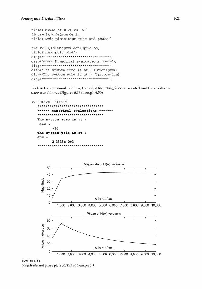
Analog and Digital Filters 621
title(‘Phase of H(w) vs. w’)figure(2);bode(num,den);title(‘Bode plots:magnitude and phase’)
figure(3);zplane(num,den);grid on;title(‘zero-pole plot’)disp(‘*********************************’);disp(‘***** Numerical evaluations *****’);disp(‘*********************************’);disp(‘The system zero is at :’);roots(num)disp(‘The system pole is at : ‘);roots(den)disp(‘*********************************’);
Back in the command window, the script fi le active_fi lter is executed and the results are shown as follows (Figures 6.48 through 6.50):
>> active _ filter*************************************** Numerical evaluations ****************************************The system zero is at : ans = -20The system pole is at : ans = -3.3333e+003*********************************
FIGURE 6.48Magnitude and phase plots of H(w) of Example 6.5.
40
30
50
01,000 2,000 3,000 4,000 5,000
Magnitude of H(w) versus w
6,000 7,000 8,000 9,000 10,000
1,000 2,000 3,000 4,000 5,000 6,000 7,000 8,000 9,000 10,000
w in rad/sec
Mag
nitu
de
20
10
60
40
20
80
0
Ang
le in
deg
rees
w in rad/sec
Phase of H(w) versus w
CRC_47760_CH006.indd 621CRC_47760_CH006.indd 621 7/23/2008 2:26:50 PM7/23/2008 2:26:50 PM

622 Practical MATLAB® Applications for Engineers
Example 6.6
Create the script fi le butt_chev that returns the magnitude and phase plots of the follow-ing analog LPFs:
a. Butterworth b. Chebyshev/type 1 c. Chebyshev/type 2
with the following fi lter’s specs:
1. The fi lter’s order of N = 5 2. Pass-band edge at Wp = 1 rad/s 3. Pass-band ripple of Rp = 1 dB 4. Stop-band ripple of Rs = 1 dB
FIGURE 6.49Bode plots of H(w) of Example 6.5.
Frequency (rad/s)
Pha
se (
in d
egre
e) T
o: Y
(1)
Bode plots:magnitude and phase
0
10
20
30
40
50From: U(1)
104103102101100 1050
20
40
60
80
100
Mag
nitu
de (
dB)
FIGURE 6.50Zero/pole plots of H(w) of Example 6.5.
−3500 −3000 −2500 −2000 −1500 −1000 −500 0
−1000
−500
0
500
1000
Real part
Imag
inar
y pa
rt
zero-pole plot
CRC_47760_CH006.indd 622CRC_47760_CH006.indd 622 7/23/2008 2:26:50 PM7/23/2008 2:26:50 PM

Analog and Digital Filters 623
MATLAB Solution% Script file: butt _ chevRp = 1 ; % in db (passband ripple)Rs = 1 ; % in db (stopband ripple)Wp = 1 ; % pass band edge % Butterworth LPF.
n = 5; % order% transfer function, But. LPF.[num1, den1] = butter (n, Wp, ‘s’);% plot the frequency response Butterworth. LPFw = [0:.1: 5];h1 = freqs (num1, den1, w);gain1 = 20 * log10 (abs (h1));
figure(1);subplot(1,3,1);plot(w,gain1);axis([0 5 -80 20]);title (‘Butterworth LPF, N = 5’) xlabel (‘ frequency w (rad/sec)’)ylabel (‘gain, db’) % Chebyshev LPF, type 1
[num2, den2] = Cheby1 ( n, Rp, Wp, ‘s’);% plot the frequency response, Chebyshev 1 LPFh2 = freqs (num2,den2,w);gain2 = 20 * log10 (abs(h2));subplot (1, 3, 2);plot (w, gain2);title (‘ Chebyshev 1 LPF, N=5’); axis([0 5 -100 20]);xlabel (‘frequency w (rad/sec)’); ylabel (‘gain, db’) % Chebyshev LPF, type 2.
Wn = 1;% cut off norm. freq.[num3, den3] = Cheby2 (n, Rs, Wn, ‘s’);h3 = freqs (num3, den3, w);gain3 = 20 * log10 (abs(h3));subplot (1, 3, 3);plot (w, gain3);title (‘Chebyshev 2 LPF, N=5’);axis([0 2 -50 10]);xlabel (‘ frequency w (rad/sec)’); ylabel (‘gain, db’)
figure(2) % Butterworth phasephase1=angle(h1);subplot(1,3,1);plot(w,phase1);axis([0 3 -4 4]);xlabel (‘freq w(rad/sec)’);ylabel(‘phase in rad’);title(‘Butterworth, phase plot’) % Chebyshev1 phasephase2=angle(h2);subplot(1,3,2)plot(w,phase2);axis([0 2 -4 4]);xlabel(‘freq w(rad/sec)’);ylabel(‘phase in rad’);title(‘Chebyshev 1, phase plot ‘) % Chebyshev2 phase
CRC_47760_CH006.indd 623CRC_47760_CH006.indd 623 7/23/2008 2:26:51 PM7/23/2008 2:26:51 PM

624 Practical MATLAB® Applications for Engineers
phase3=angle(h3);subplot(1,3,3);plot(w,phase3);axis([0 3 -2 2]);xlabel(‘freq w(rad/sec)’);ylabel(‘phase in rad’);title(‘Chebyshev 2, phase plot’)
Back in the command window, the script fi le butt_chev is executed and the magnitude and phase plots are shown in Figures 6.51 and 6.52.
FIGURE 6.51Magnitude plots of the analog LP Butterworth, Chebyshev/type-1, and Chebyshev/type-2 fi lters of Example 6.6.
20Butterworth LPF, N 5
10
10
20
30
40
50
60
70
800 5
frequency w (rad/s)
0
gain
, db
0 5frequency w (rad/s)
20Chebyshev 1 LPF, N 5
20
40
60
80
100
0
gain
, db
0 1 2frequency w (rad/s)
Chebyshev 2 LPF, N 510
10
20
30
40
50
0
gain
, db
FIGURE 6.52Phase plots of the analog LP Butterworth, Chebyshev/type-1, and Chebyshev/type-2 fi lters of Example 6.6.
Butterworth, phase plot4
3
2
1
phas
e in
rad
0
1
2
3
410 2 3
freq w (rad/s)
Chebyshev 1, phase plot4
3
2
1
phas
e in
rad
0
1
2
3
40 1 2
freq w (rad/s)
Chebyshev 2, phase plot2
1.5
1
0.5
0
1
2
phas
e in
rad
0 31 2
freq w (rad/s)
0.5
1.5
CRC_47760_CH006.indd 624CRC_47760_CH006.indd 624 7/23/2008 2:26:51 PM7/23/2008 2:26:51 PM

Analog and Digital Filters 625
Example 6.7
Create the script fi le analog_digital that returns the following:
a. The third-order normalized analog low-pass Butterworth fi lter’s magnitude and phase plots of H(w).
b. Use lp2lp to transform the normalized fi lter of part (a) to an analog LPF with wc = 3 rad/s, and obtain the magnitude and phase plots of H(w).
c. With a sampling rate of T = 0.3 obtain the numerator and denominator coeffi cients of the discrete IIR transfer function H(z) fi lter for wc = 3 rad/s of part (b).
d. Obtain its zero/pole plot of H(z) of part (c) and verify that the system implementa-tion is stable.
e. Obtain its zero/pole plot of H(s) of part (b) and verify that the system is stable and the three analog poles map into the three discrete poles of H(z).
f. Obtain the magnitude and phase plots of the discrete transfer function H(z).
MATLAB Solution% Script file: analog _ digital[z,p,k] = buttap(3); % create an analog normalized filter [Pn,Qn]= zp2tf (z,p,k); % analog normalized transfer functionT=.3;Wc=3;[Pa,Qa]=lp2lp(Pn,Qn,Wc);w =-5:.1:5;h = freqs(Pn,Qn,w);
figure(1)subplot (1,2,1) % plot of normalized butt. LPFplot (w, abs(h));axis([-5 5 0 1.2]);title (‘ Mag.analog norm. LPF’)xlabel (‘w in rad/sec’)ylabel (‘Magnitude’)subplot (1,2,2)plot(w,angle(h))xlabel (‘w in rad/sec’)ylabel (‘angle’)title(‘Phase analog norm LPF’)
figure(2)subplot (1,2,1) % plot of LPF, wc =3h2 = freqs(Pa,Qa,w);plot (w, abs(h2));title (‘ Mag. of LPF with wc=3’)xlabel (‘w in rad/sec’)ylabel (‘magnitude ‘); axis([-5 5 0.2 1.1]);subplot (1,2,2)
CRC_47760_CH006.indd 625CRC_47760_CH006.indd 625 7/23/2008 2:26:52 PM7/23/2008 2:26:52 PM

626 Practical MATLAB® Applications for Engineers
phase2=angle(h2)*180/pi;plot (w, phase2)title (‘Phase of LPF with wc=3’)xlabel (‘w in rad/sec’)ylabel (‘degrees’)[Pz,Qz]=bilinear (Pa,Qa,1/T); % discrete transfer function disp(‘******************************************’)disp(‘**************RESULTS******************* ‘) disp(‘*******************************************’) disp(‘Digital filter /numerator coefficients of the transfer function :’)disp(Pz)disp(‘ Digital filter / denominator coefficients of the transfer func-tion :’)disp(Qz)disp(‘*******************************************’)
figure(3); zplane (Pz,Qz)title (‘zero-pole plot of H(z)’)
figure(4);pzmap(Pa,Qa)title (‘zero-pole plot of H(s)’)
figure(5)[magz, phasez] = freqz (Pz, Qz, w*T/pi);subplot (1,2,1) % digital filterplot (w*T, magz)xlabel (‘W in rad’); title(‘Mag.of digital filter H(Z)’)ylabel (‘magnitude’);axis([-2 2 0.4 1.1]);subplot(1,2,2)plot(w*T,phasez*180/pi)xlabel(‘W in rad’); ylabel(‘degrees’);title(‘Phase of digital filter H(z)’)
Back in the command window, the script fi le analog_digital is executed and the results are shown as follows (Figures 6.53 through 6.57):
>> analog _ digital********************************************************RESULTS*************************************************************Digital filter /numerator coefficients of the transfer function : 0.0380 0.1141 0.1141 0.0380Digital filter / denominator coefficients of the transfer function : 1.0000 -1.3445 0.8215 -0.1727*******************************************
CRC_47760_CH006.indd 626CRC_47760_CH006.indd 626 7/23/2008 2:26:52 PM7/23/2008 2:26:52 PM
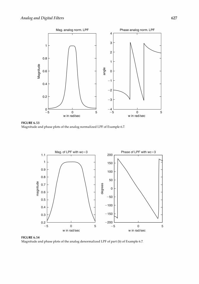
Analog and Digital Filters 627
FIGURE 6.54Magnitude and phase plots of the analog denormalized LPF of part (b) of Example 6.7.
1.1Mag. of LPF with wc3
1
0.9
0.8
0.7
0.4
0.3
0w in rad/sec
550.2
mag
nitu
de
0.6
0.5
w in rad/sec
200
150
100
50
0
50
100
150
200Phase of LPF with wc3
degr
ees
0 55
FIGURE 6.53Magnitude and phase plots of the analog normalized LPF of Example 6.7.
1
Mag. analog norm. LPF
0 5w in rad/sec
5
0.6
0.8
0.4
0.2
0
Mag
nitu
de
4
3
2
1
0
1
2
3
4
Phase analog norm. LPF
w in rad/sec0 55
angl
e
CRC_47760_CH006.indd 627CRC_47760_CH006.indd 627 7/23/2008 2:26:52 PM7/23/2008 2:26:52 PM

628 Practical MATLAB® Applications for Engineers
FIGURE 6.55Zero/pole plot of the discrete IIR transfer function H(z) for wc = 3 rad/s of part (b) of Example 6.7.
1
zero-pole plot of H(z)
0.8
0.6
0.4
0.2
3
0.2
0.4
0.6
0.8
1
1 0.5 0 0.5 1Real part
0
Imag
inar
y pa
rt
FIGURE 6.56Zero/pole plot of the analog transfer function H(s) for wc = 3 rad/s of part (b) of Example 6.7.
3zero-pole plot of H(s)
2
1
0
1
2
33 2.5 2 1.5 1 0.5 0
Real axis
Imag
inar
y ax
is
CRC_47760_CH006.indd 628CRC_47760_CH006.indd 628 7/23/2008 2:26:53 PM7/23/2008 2:26:53 PM

Analog and Digital Filters 629
Example 6.8
Create the script fi le direc_butt_disig that solves Example 6.7 by directly obtaining the magnitude and phase plots of the discrete transfer function H(z) (LPF third order, with T = 0.3 and a cutoff frequency of wc = 3 rad/s).
% Script file : direc _ butt _ disign =3;T=.03;wc=3;w =-5:.1:5;wz = w*T;[Pz,Qz] = butter(n,wc*T/pi);[magz,phasez]=freqz(Pz,Qz,wz/pi);subplot(1,2,1)plot(wz,magz);title(‘Mag. of digital LPF’);axis([-5 5 0.4 1.1]);xlabel(‘w in rad’)ylabel(‘magnitude’)subplot(1,2,2)plot(wz,phasez*180/pi);title(‘Phase of digital LPF vs w’)xlabel(‘w in rad’)ylabel(‘phase in degrees’)
Back in the command window, the script fi le direc_butt_disig is executed and the results are shown as follows (Figure 6.58):
>> direc _ butt _ disig
FIGURE 6.57Magnitude and phase plots of H(z) of Example 6.7.
Mag. of digital filter H(z)
1
0.9
0.8
0.7mag
nitu
de
0.6
0.5
1.1
0.42 1 0 1 2
W in rad
Phase of digital filter H(z)30
20
10
10
20
302 1 0 1 2
W in rad
0
degr
ees
CRC_47760_CH006.indd 629CRC_47760_CH006.indd 629 7/23/2008 2:26:53 PM7/23/2008 2:26:53 PM
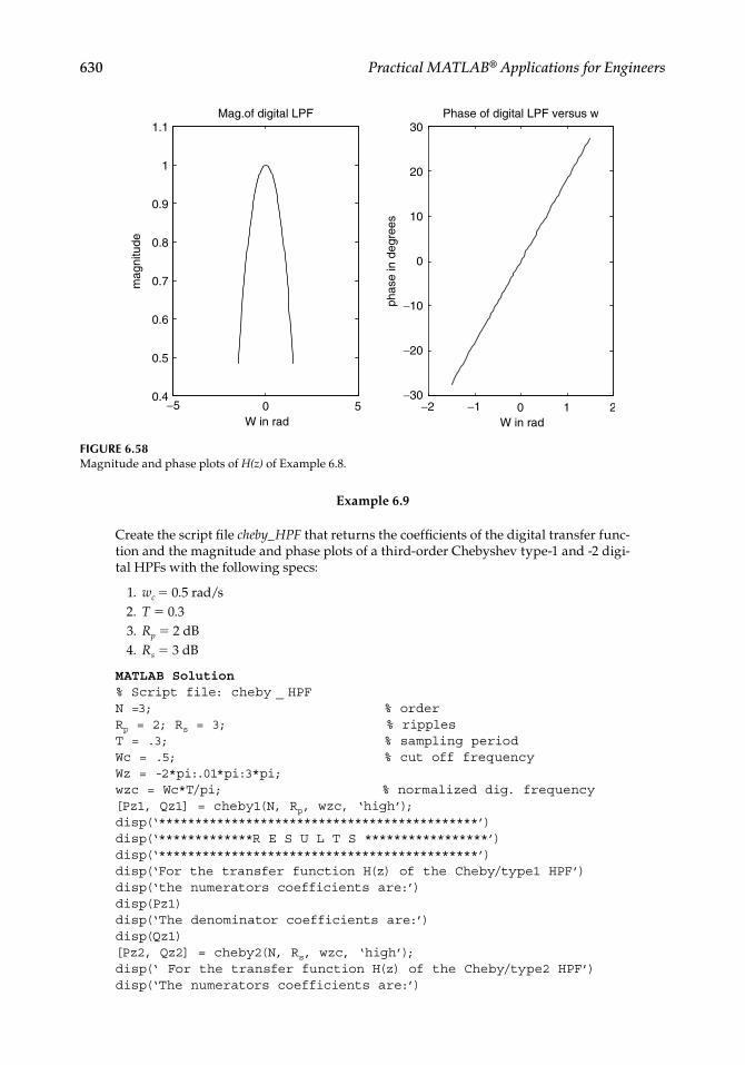
630 Practical MATLAB® Applications for Engineers
Example 6.9
Create the script fi le cheby_HPF that returns the coeffi cients of the digital transfer func-tion and the magnitude and phase plots of a third-order Chebyshev type-1 and -2 digi-tal HPFs with the following specs:
1. wc = 0.5 rad/s 2. T = 0.3 3. Rp = 2 dB 4. Rs = 3 dB
MATLAB Solution% Script file: cheby _ HPFN =3; % orderRp = 2; Rs = 3; % ripplesT = .3; % sampling periodWc = .5; % cut off frequencyWz = -2*pi:.01*pi:3*pi;wzc = Wc*T/pi; % normalized dig. frequency[Pz1, Qz1] = cheby1(N, Rp, wzc, ‘high’);disp(‘********************************************’)disp(‘*************R E S U L T S *****************’)disp(‘********************************************’)disp(‘For the transfer function H(z) of the Cheby/type1 HPF’)disp(‘the numerators coefficients are:’)disp(Pz1)disp(‘The denominator coefficients are:’)disp(Qz1)[Pz2, Qz2] = cheby2(N, Rs, wzc, ‘high’); disp(‘ For the transfer function H(z) of the Cheby/type2 HPF’)disp(‘The numerators coefficients are:’)
FIGURE 6.58Magnitude and phase plots of H(z) of Example 6.8.
−5 0 50.4
0.5
0.6
0.7
0.8
0.9
1
1.1Mag.of digital LPF
mag
nitu
de
−2 −1 0 1 2−30
−20
−10
0
10
20
30Phase of digital LPF versus w
W in radW in rad
phas
e in
deg
rees
CRC_47760_CH006.indd 630CRC_47760_CH006.indd 630 7/23/2008 2:26:53 PM7/23/2008 2:26:53 PM

Analog and Digital Filters 631
disp(Pz2)disp(‘The denominator coefficients are:’); disp(Qz2)disp(‘********************************************’)[mag1, phase1] = freqz (Pz1,Qz1,Wz);[mag2, phase2] = freqz (Pz2,Qz2,Wz);subplot (2,2,1)plot (Wz, mag1)title (‘Mag of Cheby. type/1, HPF’);axis([0 5 0 1.1]);xlabel (‘ W in rad’)ylabel (‘Magnitude’)subplot (2,2,2)plot (Wz, phase1* 180/pi)title (‘Phase of Cheby. type/1,HPF ‘)ylabel (‘Angle in degrees’)xlabel (‘ W in rad’)subplot (2,2,3)plot (Wz, mag2)title (‘Mag.of Cheby. type/2, HPF’); axis([0 1 0 1.5]); xlabel (‘W in rad’); ylabel (‘Magnitude’)subplot (2,2,4)plot (Wz, phase2 * 180/ pi); xlabel (‘W in rad’)ylabel (‘Angle in degrees’)title(‘Phase. of Cheby. type/2, HPF’)disp(‘****** FILTERS TRANSFER FUNCTIONS*******’) disp(‘********************************************’)disp(‘Chebyshev type 1’)tf(Pz2,Qz2,T)disp(‘ ^^^^^^^^^^^^^^^^^ ’)disp(‘Chebyshev type 2’)tf(Pz1,Qz1,T)disp(‘****************************************************’)
The script fi le cheby_HPF is executed and the results are shown as follows (Figure 6.59):
>> cheby _ HPF
********************************************************* R E S U L T S ***********************************************************For the transfer function H(z) of the Cheby/type1 HPFthe numerators coefficients are: 0.8006 -2.4019 2.4019 -0.8006
The denominator coefficients are: 1.0000 -2.5767 2.2067 -0.6217
For the transfer function H(z) of the Cheby/type2 HPFThe numerators coefficients are: 0.9564 -2.8530 2.8530 -0.9564
The denominator coefficients are: 1.0000 -2.8943 2.8098 -0.9147
CRC_47760_CH006.indd 631CRC_47760_CH006.indd 631 7/23/2008 2:26:54 PM7/23/2008 2:26:54 PM

632 Practical MATLAB® Applications for Engineers
*************************************************FILTERS TRANSFER FUNCTIONS ******************************************************Chebyshev type 1
Transfer function:0.8006 z^3 - 2.402 z^2 + 2.402 z - 0.8006----------------------------------------- z^3 - 2.577 z^2 + 2.207 z - 0.6217
Sampling time: 0.3^^^^^^^^^^^^^^^^^^^Chebyshev type 2
Transfer function:0.9564 z^3 - 2.853 z^2 + 2.853 z - 0.9564----------------------------------------- z^3 - 2.894 z^2 + 2.81 z - 0.9147
Sampling time: 0.3****************************************************
FIGURE 6.59Magnitude and phase plots of Chebyshev type-1 and -2 digital HPFs of Example 6.9.
1
Mag. of Cheby. type/1, HPF
0.8
0.6
W in rad
0.4Mag
nitu
de
0.2
00 1 2 3 4 5
Phase of Cheby. type/1, HPF600
400
200
0
Ang
le in
deg
rees
0 5 10
W in rad
200
40010 5
Phase of Cheby. type/2, HPF600
400
200
0
200
40010 5 0 5 10
Ang
le in
deg
rees
W in rad
Mag. of Cheby. type/2, HPF1.5
1
0.5
00 0.5 1
W in rad
Mag
nitu
de
CRC_47760_CH006.indd 632CRC_47760_CH006.indd 632 7/23/2008 2:26:54 PM7/23/2008 2:26:54 PM

Analog and Digital Filters 633
Example 6.10
Test the Butterworth LP digital fi lter of Example 6.7 by applying as an input the signal x(t) = 2 + cos(0.2 * t) + cos(4 * t ) sampled every T = 0.3 s.
Create the script fi le inp_out that returns the following plots:
a. x(t) versus t b. y(t) versus t c. x(nT) versus nT d. y(nT) versus nT
where y denotes the fi lter’s output.
MATLAB Solution% Script file: inp _ outPz = [0.0380 0.1141 0.1141 0.0380];Qz = [1.0000 -1.3445 0.8215 -0.172];n = 0:1:100; %Discrete time sequenceT = 0.3;input = 2 + cos(0.2*T.*n)+cos(4*T.*n);output= filter(Pz,Qz,input);t = 0:.05:8; % time rangeinputa = 2 + cos(0.2.*t) + cos(4.*t);subplot(2,2,1)plot(t,inputa)xlabel(‘t in sec’)ylabel(‘Amplitude’)title(‘[x(t) = 2 + cos(0.2.*t) + cos (4.*t)] vs. t’)axis([0 5 0 5])subplot(2,2,2)plot(n*T,output)xlabel(‘t in sec’)ylabel(‘Amplitude’)title(‘y(t) vs. t’);axis([0 8 0 4])subplot(2,2,3)stem(n*T,input)xlabel(‘time index nT’)ylabel(‘Amplitude’)title(‘x(nT) vs. nT’);axis([0 5 0 5])subplot(2,2,4)stem(n*T,output)xlabel(‘time index nT’)ylabel(‘Amplitude’)title(‘y(nT) vs. nT’);axis([0 8 0 4])
The script fi le inp_out is executed and the results are shown in Figure 6.60.
>> inp _ out
Note that the fi lter’s output presents a high DC component plus the low frequency of the input with some traces of the high frequency.
CRC_47760_CH006.indd 633CRC_47760_CH006.indd 633 7/23/2008 2:26:54 PM7/23/2008 2:26:54 PM

634 Practical MATLAB® Applications for Engineers
Example 6.11
Create the script fi le Cheby_1_2 that tests the design of the Chebyshev/types 1 and 2 HO digital fi lter of Example 6.9 and returns their outputs by applying as input the signal x(t) = 2 + cos(0.2 * t) + cos(0.5 * t) sampled at the rate T = 0.3.
a. Obtain plots of each component of x(t). b. Obtain plots of the discrete input signal and the corresponding fi lter’s outputs. c. Analyze and discuss each fi lter’s output and state which of the two has a better
performance.
MATLAB Solution% Script file: Cheby _ 1 _ 2,Pz1 = [0.8006 -2.4019 2.4019 -0.8006]; % num. and den. of digital filter type 1Qz1 = [1.0000 -2.5767 2.2067 -0.6217];Pz2 = [0.9564 -2.8530 2.8530 -0.9564]; % num. and den. of digital filter type 2Qz2 = [1.0000 -2.8943 2.8098 -0.9147];n = 0:1:300; % discrete time sequenceT = 0.3;Dc = 2.*ones(1,301);f1 = 2*cos(.2*T.*n);f2 = cos(.5*T.*n);figure(1)subplot(3,1,1)plot(n*T,dc);
FIGURE 6.60Analog and discrete fi lter’s input and output of Example 6.10.
5[x(t) 2 cos (0.2.*t ) cos (4. *t )] versus t
4
3
2
1
0 1 2 3 4 5
t in sec
Am
plitu
de
0
Am
plitu
de
4
3
2
1
00 2 4 6 8
t in sec
y(t) versus t
00
1
2
3
4
5x(nT) versus nT
Am
plitu
de
1 2 3time index nT
4 5
y(nT) versus nT
time index nT0 2 4 6 8
4
3
2
1
0
Am
plitu
de
CRC_47760_CH006.indd 634CRC_47760_CH006.indd 634 7/23/2008 2:26:54 PM7/23/2008 2:26:54 PM

Analog and Digital Filters 635
ylabel(‘Input:DC component’);subplot(3,1,2)plot(n*T,f1);ylabel(‘Input:2cos(0.2 t)’);subplot(3,1,3)plot(n*T,f2);ylabel(‘Input:cos(0.5t)’);xlabel(‘time’)figure(2)input = 2.*ones(1,301) + 2*cos(.2*T.*n) + cos(.5*T.*n);output1 = filter(Pz1,Qz1,input);output2 = filter(Pz2,Qz2,input);subplot(3,1,1)plot(n*T,input), hold on; stem(n*T,input)ylabel(‘Input sequence’)subplot(3,1,2);plot(n*T,output1); hold on; stem(n*T,output1);ylabel(‘Outputs Chev 1’)subplot(3,1,3);plot(n*T,output2);hold on;stem(n*T,output2)ylabel(‘Outputs Chev 2’)xlabel(‘nT’);
The script fi le Cheby_1_2 is executed and the results are shown in Figures 6.61 and 6.62.
FIGURE 6.61Component plots of the input of x(t) of Example 6.11.
2
1
Inpu
t: D
C c
ompo
nent 3
0 10 20 4030 50 60 70 80 90
Inpu
t: co
s(0
.5t)
10 10 20 30 40 50
time
60 70 80 90
0
1
Inpu
t: 2c
os(0
.2t) 2
20 10 20 30 40 50 60 70 80 90
0
CRC_47760_CH006.indd 635CRC_47760_CH006.indd 635 7/23/2008 2:26:55 PM7/23/2008 2:26:55 PM

636 Practical MATLAB® Applications for Engineers
Note that the output of the Cheby type-1 fi lter is truly an HPF (only the frequency w = 0.5 is present), whereas the output of the Cheby type-2 fi lter is similar to the compos-ite input signal in which the two input frequencies are present.
Example 6.12
Example 6.12 involves an FIR fi lter, type 1 with symmetry, and length N = odd. Obtain by hand expressions of the amplitude and phase of H(ejW), verifying that the phase is linear if the impulse response sequence is given by
h(n) = [.5 1 .5] for n = 0, 1, and 2
ANALYTICAL Solution
H e h n z e ejW
n
nn jW j W( ) ( ) . .
0
220 5 1 0 5∑
H e e e ejW jW jW jW( ) [ . . ] 0 5 0 5
H e W ejW jW( ) [ cos ] 1
H e W WjW( ) cos 1 for
∠H e WjW( ) for
FIGURE 6.62Plots of the discrete input and the fi lter’s outputs of Example 6.11.
5
5
0In
put s
eque
nce
0 10 20 30 40 50 60 70 80 90
5
5
0
Out
put C
hev
1
0 10 20 30 40 50 60 70 80 90
5
5
0
Out
put C
hev
2
nT0 10 20 30 40 50 60 70 80 90
CRC_47760_CH006.indd 636CRC_47760_CH006.indd 636 7/23/2008 2:26:55 PM7/23/2008 2:26:55 PM

Analog and Digital Filters 637
Example 6.13
Given the following impulse response sequence: hn = [−5 2 3 4 2 −1 3 −1 2 4 3 2 −5] that corresponds to a digital fi lter.
Determine the following:
a. The type of fi lter b. By hand calculate its frequency response c. Create the script fi le Fir_typ1_1 that returns the following plots:
i. h(n) versus n ii. The fi rst seven a(n)’s terms of H(W), in a tablelike format, and verify the results
obtained in part (b) iii. H(W) versus W iv. Zero–pole
ANALYTICAL Solution
Clearly, h(n) = h(N − 1 − n) is a symmetric sequence with N = odd (13), then the fi lter is an FIR type 1. Then from R.6.120
H W a n nW
n1 1
0
6
( ) ( )cos( )
∑
where
a1(0) = h(6) = 3
a1(1) = 2h(6 − 1) + 2h(5) = 2(−1) = −2
a1(2) = 2h(6 − 2) = 2h(4) = 2(2) = 4
a1(3) = 2h(6 − 3) = 2h(3) = 2(4) = 8
a1(4) = 2h(6 − 4) = 2h(2) = 2(3) = 6
a1(5) = 2h(6 − 5) = 2h(1) = 2(2) = 4
a1(6) = 2h(6 − 6) = 2h(0) = 2(−5)
a1(6) = −10
Then
H1(w) = a1(0) + a1(1) cos(W) + a1(2) cos(2W) + a1(3)cos(3W)
+ a1(4)cos(4W) + a1(5)cos(5W) + a1(6)cos(6W)
H1(ω) = 3 − 2cos(W) + 4cos(2W) + 8cos(3W) + 6cos(4W) + 4cos(5W) − 10cos(6W)
MATLAB Solution% Script file : Fir _ typ1 _ 1h = [-5 2 3 4 2 -1 3 -1 2 4 3 2 -5];N = length(h);n = 0:N-1;mid = (N-1)/2;disp(‘****coeff. of H1(w)****’)disp(‘index n coeff. a(n)‘)a = [h(mid+1) 2*h(mid:-1:1)]; % generates the a’s coeff.nn = (0:6)’;
CRC_47760_CH006.indd 637CRC_47760_CH006.indd 637 7/23/2008 2:26:55 PM7/23/2008 2:26:55 PM

638 Practical MATLAB® Applications for Engineers
aa = a(1:7)’;[nn aa]disp(‘*********************’)m = 0:1:mid;w = -pi:.01*pi:pi;subplot(2,2,1)stem(n,h)axis([0 15 -6 5])xlabel(‘time index n’)ylabel(‘Amplitude ‘)title(‘[Impulse sequence h(n)] vs. n’)subplot(2,2,2)stem(0:mid,a)xlabel(‘ index n’)ylabel(‘Amplitude’)title(‘[coeff. a1(n)] vs. n’)H1 = a(1)+a(2)*cos(w)+a(3)*cos(2*w)+a(4)*cos(3*w)+a(5)*cos(4*w);H2 = a(6)*cos(5*w)+a(7)*cos(6*w);H = H1+H2;subplot(2,2,3)plot(w,H)xlabel(‘W‘);ylabel(‘Amplitude’)title(‘H1(W) vs. W’)subplot(2,2,4)zplane(h,1)title(‘zero-pole plot’)
The script fi le Fir_typ1_1 is executed and the results are shown as follows:
>> Fir _ typ1 _ 1
****coeff. of H1(w)**** index n coeff. a(n) ans = 0 3 1 -2 2 4 3 8 4 6 5 4 6 -10**********************
Example 6.14
Create the script fi le fi lter_wind that returns the normalized LP-FIR fi lters using the command fi r1 in conjunction with the following windows:
a. Kaiser (β = 3.5) b. Hanning c. Blackman d. Hamming e. Triangular f. Bartlett
The fi lter’s specs are N = 64 and Rp = 1.4 dB.
CRC_47760_CH006.indd 638CRC_47760_CH006.indd 638 7/23/2008 2:26:56 PM7/23/2008 2:26:56 PM

Analog and Digital Filters 639
MATLAB Solution% Script file: filter _ windformat longhnk = fir1(64,.4,kaiser(65,3.5));[h1,w1] = freqz(hnk,1,256);magk = 20*log10(abs(h1));subplot(3,2,1)plot(w1,magk)title(‘Filter using kaiser win.’)ylabel(‘gain in db’)subplot(3,2,2)hnhan = fir1(64,.4,hanning(65));[h2,w2] = freqz(hnhan,1,256);maghan = 20*log10(abs(h2));plot(w2,maghan)title(‘Filter using hanning win.’)ylabel(‘gain in db’)subplot(3,2,3)hnbla = fir1(64,.4,blackman(65));[h3,w3] = freqz(hnbla,1,256);magblac=20*log10(abs(h3));plot(w3,magblac)title(‘Filter using blackman win.’)ylabel(‘gain in db’)subplot(3,2,4)% hamming window is the default
FIGURE 6.63Filter’s plots of Example 6.13.
4
[Impulse sequence h(n)] versus n
2
0
0 5 10
time n n
15
Am
plitu
de
2
4
6
[coeff. a1(n)] versus n10
5
0
20 4 6
Am
plitu
de
5
10
0 1
12
Real part
Imag
inar
y pa
rt
zero-pole plot1
0.5
0.5
1
1
0
20
10
0
10
20
304 2 0 2 4
W
H1(W) versus W
Am
plitu
de
time index n Index n
CRC_47760_CH006.indd 639CRC_47760_CH006.indd 639 7/23/2008 2:26:56 PM7/23/2008 2:26:56 PM

640 Practical MATLAB® Applications for Engineers
hnham = fir1(64,.4);[h4,w4] = freqz(hnham,1,256);magham = 20*log10(abs(h4));plot(w4,magham)title(‘Filter using hamming win.’)ylabel(‘gain in db’)subplot(3,2,5)hntri = fir1(64,.4,triang(65));[h5,w5] = freqz(hntri,1,256);magtri = 20*log10(abs(h5));plot(w5,magtri)title(‘Filter using triang. win.’)xlabel(‘frequency in rad.’)ylabel(‘gain in db’)axis([0 3 -60 10])subplot(3,2,6)hnbar = fir1(64,.4,bartlett(65));[h6,w6] = freqz(hnbar,1,256);magbar = 20*log10(abs(h6));plot(w6,magbar)title(‘Filter using bartlett win.’)xlabel(‘frequency in rad.’)ylabel(‘gain in db’)axis([0 3 -60 10])
The script fi le fi lter_wind is executed and the results are shown in Figure 6.64.
FIGURE 6.64Normalized LP FIR fi lters’ plots using fi r1 with the window arguments of Example 6.14.
100
200
100
0
0
gain
in d
b
1 2 3 4
Filter using blackman win.
frequency in rad
gain
in d
b
100
200
100
0
0 1 2 3 4
Filter using hamming win.
frequency in rad
Filter using bartlett win.
gain
in d
b
40
60
0
20
0 1 2 3
frequency in rad
gain
in d
b
100
100
2000
0
1 2
Filter using hanning win.
3 4
frequency in rad
100
100
2000
0
gain
in d
b
1 2
Filter using kaiser win.
3 4
frequency in rad
40
60
0
20
gain
in d
b
0 1 2 3
Filter using triang. win.
frequency in rad
CRC_47760_CH006.indd 640CRC_47760_CH006.indd 640 7/23/2008 2:26:56 PM7/23/2008 2:26:56 PM

Analog and Digital Filters 641
Example 6.15
Create the script fi le multiban that returns the realization of a digital multiband nor-malized fi lter with the specs indicated by the sketch shown in Figure 6.65, using the following functions:
a. fi r2 of order 50, with a Bartlett window (FIR) b. remez (FIR) of order 50 c. yulewalk digital IIR of order 15
MATLAB Solution% Script File: multibanw = [0 .1 .2 .3 .4 .5 .6 .7 .8 1];mag = [0 0 1 1 0 0 1 1 0 0];hnfir = fir2(50,w,mag,bartlett(51));[h1, w1] = freqz(hnfir,1,256);subplot (3,1,1)plot (w1/pi, abs(h1))ylabel (‘gain‘)title (‘Multiban filter using fir2 (with bartlett window)’)xlabel(‘frequency W (in rad)’)subplot (3,1,2)hnrem = remez(50,w,mag);[h2, w2] = freqz (hnrem,1,256);plot (w2/pi, abs(h2))ylabel (‘gain‘)title (‘Multiban filter using remez’)xlabel(‘frequency W (in rad)’)subplot(3,1,3)[num,den] = yulewalk(15,w,mag);[hiir,w] = freqz(num,den,256);plot(w/(pi),abs(hiir))ylabel (‘gain’)title (‘Multiban filter using yulewalk’)xlabel(‘frequency W (in rad)’)
The script fi le multiban is executed and the results are as follows (Figure 6.66):
>> multiban
FIGURE 6.65Filter’s specs of Example 6.15.
H(W )
0
W (rad.)
1
.2 .4 .6 .8 1.0
CRC_47760_CH006.indd 641CRC_47760_CH006.indd 641 7/23/2008 2:26:57 PM7/23/2008 2:26:57 PM
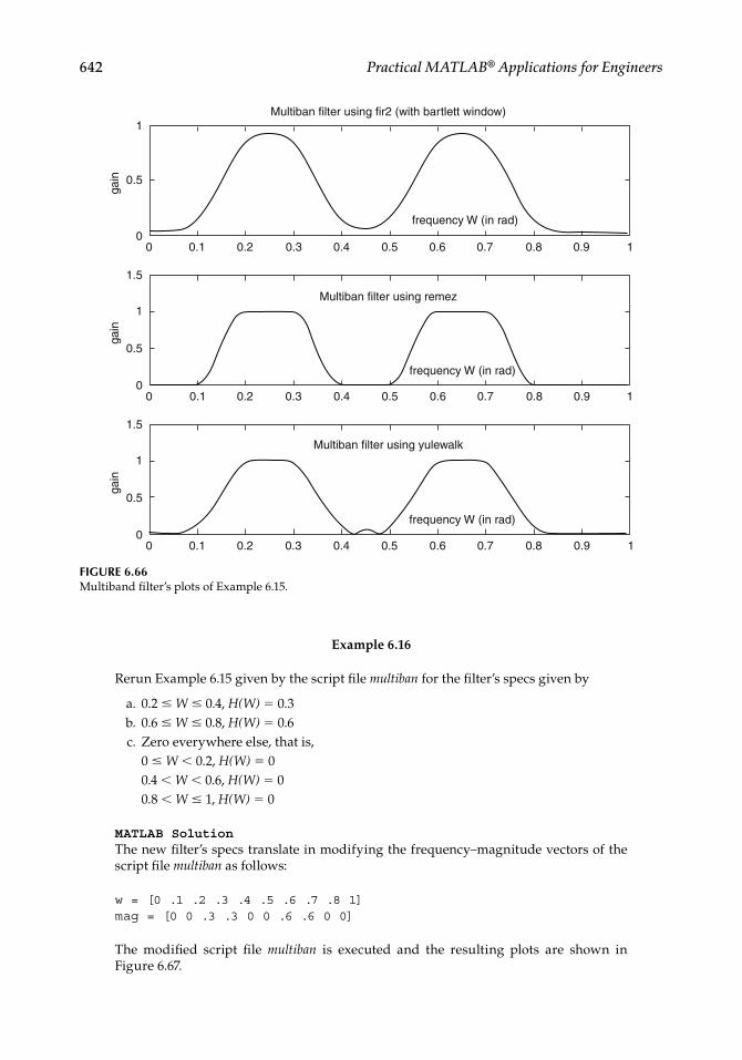
642 Practical MATLAB® Applications for Engineers
Example 6.16
Rerun Example 6.15 given by the script fi le multiban for the fi lter’s specs given by
a. 0.2 ≤ W ≤ 0.4, H(W) = 0.3 b. 0.6 ≤ W ≤ 0.8, H(W) = 0.6 c. Zero everywhere else, that is, 0 ≤ W < 0.2, H(W) = 0 0.4 < W < 0.6, H(W) = 0 0.8 < W ≤ 1, H(W) = 0
MATLAB SolutionThe new fi lter’s specs translate in modifying the frequency–magnitude vectors of the script fi le multiban as follows:
w = [0 .1 .2 .3 .4 .5 .6 .7 .8 1]mag = [0 0 .3 .3 0 0 .6 .6 0 0]
The modifi ed script fi le multiban is executed and the resulting plots are shown in Figure 6.67.
FIGURE 6.66Multiband fi lter’s plots of Example 6.15.
00 0.1 0.2 0.3 0.4 0.5 0.6
Multiban filter using fir2 (with bartlett window)
Multiban filter using remez
Multiban filter using yulewalk
frequency W (in rad)
frequency W (in rad)
frequency W (in rad)
0.7 0.8 0.9 1
0.5
gain
gain
gain
1
00 0.1 0.2 0.3 0.4 0.5 0.6 0.7 0.8 0.9 1
1
0.5
1.5
0
1
0.5
1.5
0 0.1 0.2 0.3 0.4 0.5 0.6 0.7 0.8 0.9 1
CRC_47760_CH006.indd 642CRC_47760_CH006.indd 642 7/23/2008 2:26:57 PM7/23/2008 2:26:57 PM

Analog and Digital Filters 643
Example 6.17
Create the script fi le butt_implem that returns a third-order analog Butterworth LPF, at the component level, with wc = 104 rad/s and a load impedance of 100 Ω.
a. Start the design with a third-order normalized prototype LPF and obtain the cor-responding magnitude and phase plots.
b. Obtain the corresponding transfer function coeffi cients and the system poles (check for stability).
c. Obtain the normalized fi lter’s transfer function. d. Use frequency and magnitude scaling to obtain the desired fi lter transfer function.
ANALYTICAL Solution
The structure chosen for the desired LP normalized, third-order fi lter prototype (see R.6.49) is the π section shown in Figure 6.68.
The transfer function is indicated as follows:
H s
L L C s L C s L L sN ( )( ) ( ) ( )
111 2
31
21 2
(6.3)
FIGURE 6.67Multiband fi lter’s plots of Example 6.16.
1
0.5
00 0.1
gain
0.2 0.3 0.4 0.5
Multiban filter using fir2 (with bartlett window)
Multiban filter using remez
Multiban filter using yulewalk
frequency W (in rad)
frequency W (in rad)
frequency W (in rad)
0.6 0.7 0.8 10.9
1
0.5
00 0.1
gain
0.2 0.3 0.4 0.5 0.6 0.7 0.8 10.9
1
0.5
00 0.1
gain
0.2 0.3 0.4 0.5 0.6 0.7 0.8 10.9
CRC_47760_CH006.indd 643CRC_47760_CH006.indd 643 7/23/2008 2:26:57 PM7/23/2008 2:26:57 PM

644 Practical MATLAB® Applications for Engineers
MATLAB Solution% Script file : butt _ implem [z,p,k] = buttap(3);disp(‘ ******* R E S U L T S ********’)disp(‘**********************************’)disp(‘the poles are :’);disp(p);[Pn,Qn] = zp2tf(z,p,k); % returns the transf. functiondisp(‘The coefficients of the numerator of Hn(s) are: ‘); disp(Pn);
disp(‘The coefficients of the denominator of Hn(s) are: ‘); disp(Qn);system = tf(Pn,Qn);systemdisp(‘**********************************’)w =-3:.1:3;hn = freqs(Pn,Qn,w);gain=20*log10(abs(hn));subplot(1,2,1)plot(w,gain)xlabel(‘w in rad/sec’)ylabel(‘gain in db’)title(‘Normalize filter/magnitude’)subplot(1,2,2)plot(w,angle(hn)*180/pi);xlabel(‘w in rad/sec’);ylabel(‘Phase in degrees’)title(‘Normalize filter/phase’)
Back in the command window the script fi le butt_implem is executed and the results are shown as follows (Figure 6.69):
>> butt _ implem
******* R E S U L T S ******** **********************************the poles are : -0.5000 + 0.8660i -0.5000 - 0.8660i -1.0000 The coefficients of the numerator of Hn(s) are: 0 0 0 1.0000The coefficients of the denominator of Hn(s) are: 1.0000 2.0000 2.0000 1.0000 Transfer function: 1---------------------s^3 + 2 s^2 + 2 s + 1*********************************************
FIGURE 6.68Filter’s structure of Example 6.17.
1 ΩC
Vo(s)Vi(s)
L1 L2
CRC_47760_CH006.indd 644CRC_47760_CH006.indd 644 7/23/2008 2:26:58 PM7/23/2008 2:26:58 PM

Analog and Digital Filters 645
The transfer function is given by
H(s)
12 2 13 2s s s
(6.4)
Equating the coeffi cients of Equation 6.3 with the coeffi cients of Equation 6.4 the follow-ing relations are obtained:
L1L2C = 1
L1C = 2
L1 + L2 = 2
Then solving for L1, L2, and C the following is obtained:
L1 = 3/2 H, L2 = 1/2 H, and C = 4/3 F
Then the normalized LPF at the component level is shown in Figure 6.70.Frequency and magnitude scaling results in
new-R0 = R * R0 = 1 * 100 = 100 Ω
L
L R01
1 04 4
2
103 1002 10
3 102
15 * *
** mH
L
L R02
2 04 4
2
10100
2 100 5 10 5 *
**. mH
C
Cw Rc
00
4 264
31
10 1043
10 1 33
**
** . F
FIGURE 6.69Normalized fi lter’s plot of Example 6.17.
0 200
150
100
50
50
100
150
2004 2 0 2 4
0
5
10
gain
in d
b
Pha
se in
deg
rees
w in rad/sec w in rad/sec
Normalize filter/magnitude Normalize filter/phase
15
20
25
304 2 2 40
CRC_47760_CH006.indd 645CRC_47760_CH006.indd 645 7/23/2008 2:26:58 PM7/23/2008 2:26:58 PM
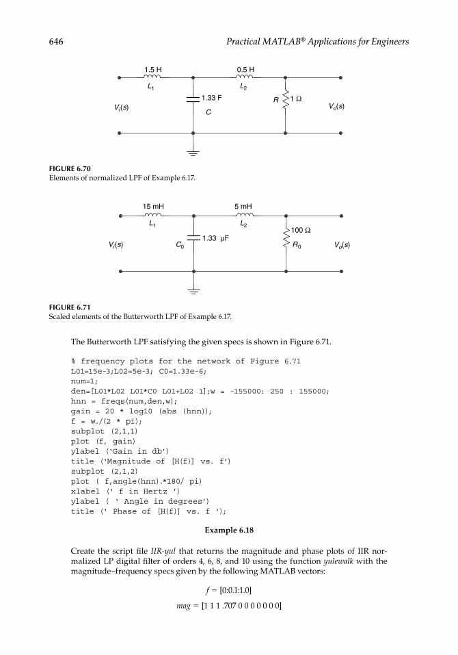
646 Practical MATLAB® Applications for Engineers
The Butterworth LPF satisfying the given specs is shown in Figure 6.71.
% frequency plots for the network of Figure 6.71L01=15e-3;L02=5e-3; C0=1.33e-6;num=1;den=[L01*L02 L01*C0 L01+L02 1];w = -155000: 250 : 155000;hnn = freqs(num,den,w);gain = 20 * log10 (abs (hnn));f = w./(2 * pi);subplot (2,1,1)plot (f, gain)ylabel (‘Gain in db’)title (‘Magnitude of [H(f)] vs. f’)subplot (2,1,2)plot ( f,angle(hnn).*180/ pi)xlabel (‘ f in Hertz ’)ylabel ( ‘ Angle in degrees’)title (‘ Phase of [H(f)] vs. f ’);
Example 6.18
Create the script fi le IIR-yul that returns the magnitude and phase plots of IIR nor-malized LP digital fi lter of orders 4, 6, 8, and 10 using the function yulewalk with the magnitude–frequency specs given by the following MATLAB vectors:
f = [0:0.1:1.0]
mag = [1 1 1 .707 0 0 0 0 0 0 0]
FIGURE 6.70Elements of normalized LPF of Example 6.17.
1.5 H
1.33 F
0.5 H
1 ΩVo(s)Vi(s)
L1
C
L2
R
FIGURE 6.71Scaled elements of the Butterworth LPF of Example 6.17.
15 mH
1.33 µF
5 mH
100 Ω
Vi(s) Vo(s)
L1
C0
L2
R0
CRC_47760_CH006.indd 646CRC_47760_CH006.indd 646 7/23/2008 2:26:59 PM7/23/2008 2:26:59 PM

Analog and Digital Filters 647
MATLAB Solution% Script file: IIR-yul% IIR/YULE-WALKER% for N = 4, 6, 8, and 10f = [0:.1:1.0];omega = 0:1/512:511/512;mag = [1 1 1 .707 zeros(1,7)];[num4,den4] = yulewalk(4,f,mag);[num6,den6] = yulewalk(6,f,mag);[num8,den8] = yulewalk(8,f,mag);[num10,den10] = yulewalk(10,f,mag);h4 = freqz(num4,den4);h6 = freqz(num6,den6);h8 = freqz(num8,den8);h10 = freqz(num10,den10);
figure(1)subplot(2,2,1)plot(f,mag,’o’,omega,abs(h4))ylabel(‘Magnitude(H)’)title(‘Order=4’)subplot(2,2,2)plot(f,mag,’o’,omega,abs(h6))ylabel(‘Magnitude(H)’)title(‘Order=6’)subplot(2,2,3)plot(f,mag,’o’,omega,abs(h8))
FIGURE 6.72Gain and phase plots of the transfer function of the fi lter of Example 6.17.
0G
ain
in d
b
50
100
150
200
2502.5 1.5 0.5 0.5 1.5 2.5
104
104
1 0
Magnitude of [H(f)] versus f
Phase of [H(f)] versus f
f in Hertz
f in Hertz
1 22
100
50
50
100
0
Ang
le in
deg
rees
2.5 1.5 0.5 0.5 1.5 2.51 0 1 22
See Figure 6.72.
CRC_47760_CH006.indd 647CRC_47760_CH006.indd 647 7/23/2008 2:26:59 PM7/23/2008 2:26:59 PM

648 Practical MATLAB® Applications for Engineers
title(‘Order=8’)ylabel(‘Magnitude(H)’);xlabel(‘W in rad’)subplot(2,2,4)plot(f,mag,’o’,omega,abs(h10))title(‘Order=10’)ylabel(‘Magnitude(H)’);xlabel(‘W in rad’)
figure(2)subplot(2,2,1)plot(omega,angle(h4)),title(‘Order=4’);ylabel(‘Angle’)subplot(2,2,2)plot(omega,angle(h6));title(‘Order=6’);ylabel(‘Angle’)subplot(2,2,3)plot(omega,angle(h8))title(‘Order=8’);xlabel(‘W in rad’);ylabel(‘Angle’)subplot(2,2,4)plot(omega,angle(h10));title(‘Order=10’)xlabel(‘W in rad’);ylabel(‘Angle’)
Back in the command window, the script fi le IIR-yul is executed and the results are shown as follows (Figures 6.73 and 6.74):
>> IIR-yul
FIGURE 6.73Magnitude plots of IIR normalized LP digital fi lter of order: 4, 6, 8, and 10 using the function yulewalk of Example 6.18.
0
1.5
0.5
Mag
nitu
de (
H)
1
010.5
Order4
0
1.5
0.5
Mag
nitu
de (
H)
1
010.5
Order6
0
1.5
0.5
Mag
nitu
de (
H)
1
010.5
Order8
W in rad W in rad0
1.5
0.5
Mag
nitu
de (
H)
1
010.5
Order10
CRC_47760_CH006.indd 648CRC_47760_CH006.indd 648 7/23/2008 2:26:59 PM7/23/2008 2:26:59 PM
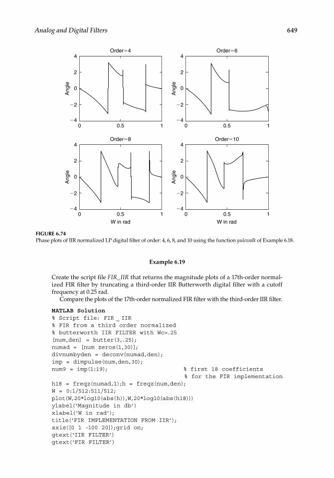
Analog and Digital Filters 649
Example 6.19
Create the script fi le FIR_IIR that returns the magnitude plots of a 17th-order normal-ized FIR fi lter by truncating a third-order IIR Butterworth digital fi lter with a cutoff frequency at 0.25 rad.
Compare the plots of the 17th-order normalized FIR fi lter with the third-order IIR fi lter.
MATLAB Solution% Script file: FIR _ IIR% FIR from a third order normalized% butterworth IIR FILTER with Wc=.25[num,den] = butter(3,.25);numad = [num zeros(1,30)]; divnumbyden = deconv(numad,den);imp = dimpulse(num,den,30);num9 = imp(1:19); % first 18 coefficients % for the FIR implementationh18 = freqz(numad,1);h = freqz(num,den);W = 0:1/512:511/512;plot(W,20*log10(abs(h)),W,20*log10(abs(h18)))ylabel(‘Magnitude in db’)xlabel(‘W in rad’);title(‘FIR IMPLEMENTATION FROM IIR’);axis([0 1 -100 20]);grid on;gtext(‘IIR FILTER’)gtext(‘FIR FILTER’)
FIGURE 6.74Phase plots of IIR normalized LP digital fi lter of order: 4, 6, 8, and 10 using the function yulewalk of Exa mple 6.18.
4
2
0
Ang
le
0 10.5
Order4
2
4
4
2
0
Ang
le
0 10.5
Order6
2
4
4
2
0
Ang
le
0 10.5
Order8
W in rad W in rad
2
4
4
2
0A
ngle
0 10.5
Order10
2
4
CRC_47760_CH006.indd 649CRC_47760_CH006.indd 649 7/23/2008 2:27:00 PM7/23/2008 2:27:00 PM

650 Practical MATLAB® Applications for Engineers
Back in the command window, the script fi le FIR_IIR is executed and the result is shown in Figure 6.75.
Example 6.20
Design the following digital fi lters:
a. An 18th-order normalized LPF with a cutoff frequency at 0.3 rad using the function fi r1, truncated by a Hamming window.
b. An 8th-order normalized BPF with a pass band between 0.3 and 0.6 rad using the function fi r1.
c. Repeat part (b) using the remez exchange algorithm that employs the Park–McClellan approach.
For each one of the preceding fi lters, return the coeffi cients of the polynomials that make up the transfer function, their transfer functions, and their respective magnitude and phase plots.
The solution is given by the script fi le designs as follows:
MATLAB Solution% Script file : designs % FIR/LPF design using fir1/part (a)coeflp = fir1(18,.3); % 18 th..order FIR filter with cutoff of .3Hlp = freqz(coeflp,1); % coef. of FIR filter
figure(1)w1= 0:1/512:511/512 ;subplot(1,2,1)plot(w1,abs(Hlp));grid on;xlabel(‘ frequency W in rad.’)
FIGURE 6.75IIR and FIR fi lter’s plots of Example 6.19.
20FIR IMPLEMENTATION FROM IIR
0
20
40
60
80
1000 0.1 0.2 0.3 0.4 0.5
W in rad0.6 0.7 0.8 0.9 1
Mag
nitu
de in
db
IIR FILTER
FIR FILTER
CRC_47760_CH006.indd 650CRC_47760_CH006.indd 650 7/23/2008 2:27:00 PM7/23/2008 2:27:00 PM

Analog and Digital Filters 651
ylabel(‘Magnitude’)title(‘Mag. of LPF using fir1/order=18’)subplot(1,2,2)plot(w1,angle(Hlp)*180/pi);grid on;xlabel(‘frequency W in rad.’)ylabel(‘Angle in degrees’)title(‘Phase of LPF using fir1/order=18’)% FIR/BPF using fir1/part(b)f = [.3 .6]; % passband regioncoefbp = fir1(8,f,’noscale’) ; % noscale, BP 8th. order filterHbp=freqz(coefbp,1);
figure(2)subplot(1,2,1)plot(w1,abs(Hbp));grid on;xlabel(‘ frequency W in rad.’)ylabel(‘Magnitude’)title(‘Mag. of BPF using fir1/order=8’)subplot(1,2,2)plot(w1,angle(Hbp)*180/pi);grid on;xlabel(‘ frequency W in rad.’)ylabel(‘Angle in degrees’)title(‘Phase of BPF using fir1/order=8’)%***********************************%FIR/BPF using remezfreq = [0 .25 .3 .6 .65 1.0]; % specifies normalized freqs.mag = [0 0 1 1 0 0];error = [2.0 1.5 2.0]; % error weights per bandnum = remez(8,freq,mag,error) ; % 8th. order BPFHrem=freqz(num,1);
figure(3)subplot(1,2,1)plot(w1,abs(Hrem));grid on;xlabel(‘frequency W in rad.’)ylabel(‘Magnitude’)title(‘Mag. of BPF using remez/order=8’)subplot(1,2,2)plot(w1,angle(Hrem)*180/pi);grid on;xlabel(‘frequency W in rad.’)ylabel(‘Angle in degrees’)title(‘Phase of BPF using remez/order=8’);den=1;disp(‘***********************************************’)disp(‘ * * * * R E S U L T S * * * * ‘)disp(‘***********************************************’) disp(‘***********************************************’) disp(‘ The coefficients of the FIR/LPF using fir1 are:’)disp(coeflp)tf(coeflp,1,-1)disp(‘***********************************************’)disp(‘ The coefficients of the FIR/BPF using fir1 are:’)disp(coefbp)
CRC_47760_CH006.indd 651CRC_47760_CH006.indd 651 7/23/2008 2:27:00 PM7/23/2008 2:27:00 PM

652 Practical MATLAB® Applications for Engineers
tf(coefbp,1,-1)disp(‘***********************************************’)disp(‘ The coefficients of the FIR/BPF using remez are:’)disp(num)tf(num,den,-1)disp(‘***********************************************’)
Back in the command window, the script fi le designs is executed, and the results are indicated as follows (Figures 6.76 through 6.78):
>> designs
*********************************************** * * * * R E S U L T S * * * * ********************************************************************************************** The coefficients of the FIR/LPF using fir1 are: Columns 1 through 8 0.0023 0.0041 0.0026 -0.0096 -0.0292 -0.0289 0.0252 0.1346 Columns 9 through 16 0.2495 0.2990 0.2495 0.1346 0.0252 -0.0289 -0.0292 -0.0096 Columns 17 through 19 0.0026 0.0041 0.0023
Transfer function: 0.002281 z^18 + 0.004063 z^17 + 0.002627 z^16 - 0.009633 z^15 - 0.02919 z^14 - 0.02889 z^13 + 0.02516 z^12 + 0.1346 z^11 + 0.2495 z^10 + 0.299 z^9 + 0.2495 z^8 + 0.1346 z^7 + 0.02516 z^6 - 0.02889 z^5
- 0.02919 z 4 - 0.009633 z^3 + 0.002627 z^2 + 0.004063 z + 0.002281
Sampling time: unspecified*********************************************** The coefficients of the FIR/BPF using fir1 are: Columns 1 through 8 0.0098 -0.0204 -0.1323 0.0391 0.3000 0.0391 -0.1323 -0.0204 Column 9 0.0098
Transfer function:0.009797 z^8 - 0.02043 z^7 - 0.1323 z 6 + 0.03912 z^5 + 0.3 z 4 + 0.03912 z^3 - 0.1323 z^2 - 0.02043 z + 0.009797
Sampling time: unspecified*********************************************** The coefficients of the FIR/BPF using remez are: Columns 1 through 8 0.1603 -0.1661 -0.3275 0.0244 0.3346 0.0244 -0.3275 -0.1661 Column 9 0.1603
Transfer function:0.1603 z^8 - 0.1661 z^7 - 0.3275 z 6 + 0.02438 z^5 + 0.3346 z 4 + 0.02438 z^3 - 0.3275 z^2 - 0.1661 z + 0.1603
Sampling time: unspecified***********************************************
CRC_47760_CH006.indd 652CRC_47760_CH006.indd 652 7/23/2008 2:27:00 PM7/23/2008 2:27:00 PM
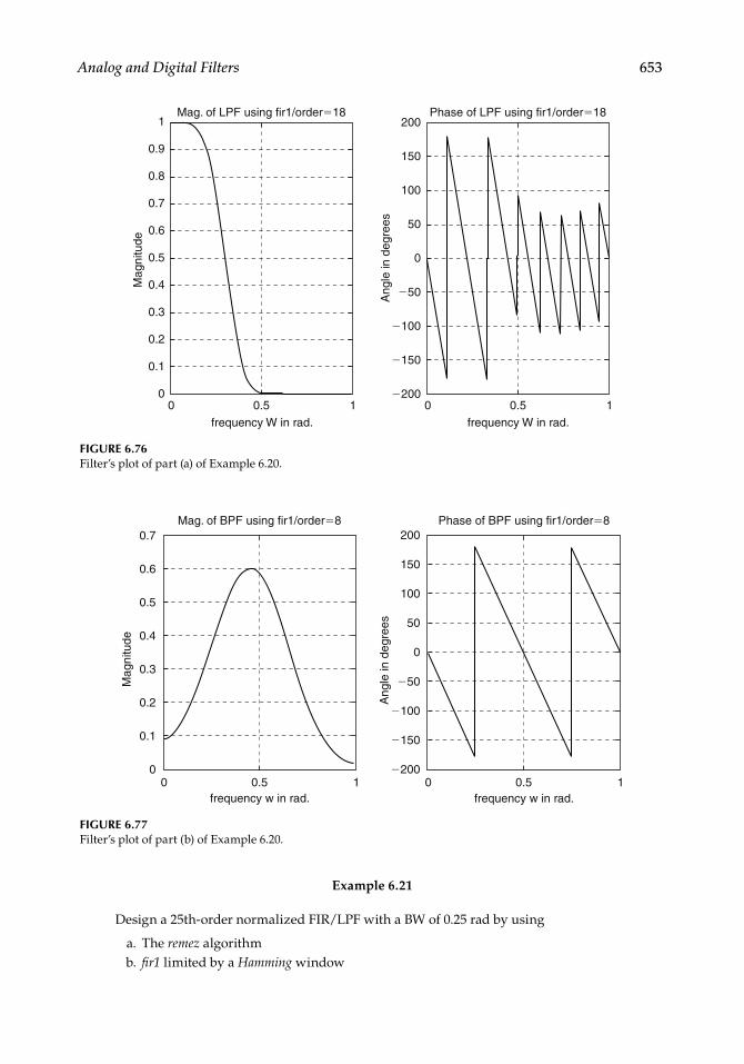
Analog and Digital Filters 653
FIGURE 6.76Filter’s plot of part (a) of Example 6.20.
200
150
100
50
50
0
100
150
200
1
0.8
Mag
nitu
de
Ang
le in
deg
rees
0.6
0.7
0.5
0.4
0.2
0.3
0.1
00 0.5
frequency W in rad.
Mag. of LPF using fir1/order18 Phase of LPF using fir1/order18
1 0 0.5
frequency W in rad.
1
0.9
FIGURE 6.77Filter’s plot of part (b) of Example 6.20.
0.7 200
150
100
50
50
100
150
200
0
0.6
0.4
Mag
nitu
de
Ang
le in
deg
rees
0.3
0.2
0.1
00 0.5
frequency w in rad.
Mag. of BPF using fir1/order8 Phase of BPF using fir1/order8
1 0 0.5frequency w in rad.
1
0.5
Example 6.21
Design a 25th-order normalized FIR/LPF with a BW of 0.25 rad by using
a. The remez algorithm b. fi r1 limited by a Hamming window
CRC_47760_CH006.indd 653CRC_47760_CH006.indd 653 7/23/2008 2:27:01 PM7/23/2008 2:27:01 PM

654 Practical MATLAB® Applications for Engineers
FIGURE 6.78Filter’s plot of part (c) of Example 6.20.
1.4 200
150
100
50
50
100
150
200
0
1.2
0.8
Mag
nitu
de
Ang
le in
deg
rees
0.6
0.4
0.2
00 0.5
frequency W in rad
Mag. of BPF using remez/order8 Phase of BPF using remez/order8
1 0 0.5frequency W in rad
1
1
For each of the fi lters obtain the magnitude and phase plots.The solution is given by the script fi le review_FIR_LPF as follows:
MATLAB Solution% Script file : review _ FIR _ LPF% Design of FIR using remezf = linspace(0,1,10);mag = [ones(1,3) .707 zeros(1,6)];Pz = remez(25,f,mag);Qz =1;Hremez = freqz(Pz,Qz);omega = 0:1/512:511/512;
figure(1)subplot(2,1,1)plot(omega,abs(Hremez))xlabel(‘frequency in rad’)ylabel(‘magnitude’)title(‘Mag./FIR using remez’)grid on;subplot(2,1,2)plot(omega,unwrap(angle(Hremez)))xlabel(‘frequency in rad’)ylabel(‘phase’)title(‘Phase/FIR using remez’)grid on;% Design of FIR using fir1/Hamming windowPz1 = fir1(25,0.3);win = hamming(26);Pz1= Pz1.*win’;Hfir1= freqz(Pz1,1);
CRC_47760_CH006.indd 654CRC_47760_CH006.indd 654 7/23/2008 2:27:01 PM7/23/2008 2:27:01 PM

Analog and Digital Filters 655
figure(2)subplot(2,1,1)plot(omega,abs(Hfir1))xlabel(‘frequency in rad’)ylabel(‘magnitude’)title(‘Mag./FIR using fir1’)grid on;subplot(2,1,2)plot(omega,unwrap(angle(Hfir1)))xlabel(‘frequency in rad’)ylabel(‘phase’); title(‘Phase/FIR using fir1’);grid on;Back in the command window, the script fi le review_FIR_LPF is executed and the results are as follows (Figures 6.79 and 6.80):>> review _ FIR _ LPF
Example 6.22
Create the script fi le revisit_analog_fi lters that returns the following fi lter imp lementations:
a. A four-pole analog Butterworth and Chebyshev/type-1 normalized fi lters with a pass-band ripple of Rp= 2 dB.
b. Transform the LPF of part (a) to an LPF with a BW of 2 rad/s using the function lp2lp.
c. Convert the Butterworth LPF of part (a) to an HPF with a cutoff frequency of 2 rad/s.
d. Convert the Butterworth LPF of part (a) to a BPF with a center frequency at 2 rad/s and a BW of 1 rad/s.
e. Convert the Butterworth and Chebyshev LPFs of part (a) to BSFs with a center fre-quency at 2 rad/s and a BW of 1 rad/s (from w = 1.5 rad/s to w = 2.5 rad/s).
FIGURE 6.79Twenty-fi fth-order normalized FIR/LPF using the remez algorithm of Example 6.21.
00
1
0.5
mag
nitu
de
1.5
0.1 0.2 0.3 0.4 0.5
Mag./FIR using remez
frequency in rad
0.6 0.7 0.8 0.9 1
020
15
10
5
0
phas
e in
rad
.
0.1 0.2 0.3 0.4 0.5
Phase/FIR using remez
frequency in rad
0.6 0.7 0.8 0.9 1
CRC_47760_CH006.indd 655CRC_47760_CH006.indd 655 7/23/2008 2:27:01 PM7/23/2008 2:27:01 PM

656 Practical MATLAB® Applications for Engineers
FIGURE 6.80Twenty-fi fth-order normalized FIR/LPF using the MATLAB fi r1 function of Example 6.21.
00
1
0.5mag
nitu
de
1.5
0.1 0.2 0.3 0.4 0.5
Mag./FIR using fir1
frequency in rad
0.6 0.7 0.8 0.9 1
025
20
15
10
5
0
phas
e in
rad
.
0.1 0.2 0.3 0.4 0.5
Phase/FIR using fir1
frequency in rad
0.6 0.7 0.8 0.9 1
MATLAB Solution % Script file: revisit _ analog _ filters % part (a) % normalize low pass filters: Butt. and Cheby.[z1,p1,k1] = buttap (4);[num1,den1] = zp2tf(z1,p1,k1);w =0:.01:6;
figure(1)subplot(2,2,1);H1= freqs(num1,den1,w);plot(w,abs(H1));ylabel(‘magnitude’)title(‘Butt. norm. LPF’)subplot(2,2,2);plot(w,angle(H1)*180/pi)ylabel(‘phase (deg)’)title(‘Butt. LPF’)[z2,p2,k2] = cheb1ap(4,2); % type 1,with 2 db passband[num2,den2] = zp2tf(z2,p2,k2);H2 = freqs(num2,den2,w);subplot(2,2,3);plot(w,abs(H2))ylabel(‘magnitude’)title(‘Cheb. norm. LPF’)xlabel(‘frequency (rad/sec)’)subplot(2,2,4);plot(w,angle(H2)*180/pi)ylabel(‘phase (deg)’)title(‘Cheb. LPF’)xlabel(‘frequency (rad/sec)’)
CRC_47760_CH006.indd 656CRC_47760_CH006.indd 656 7/23/2008 2:27:02 PM7/23/2008 2:27:02 PM

Analog and Digital Filters 657
figure(2)[num3,den3] = lp2lp(num1,den1,2); %. transf function /ButtH3 = freqs(num3,den3,w);subplot(2,2,1)plot(w,abs(H3));ylabel(‘magnitude’)title(‘Butt. LPF ,wp=2’)subplot(2,2,2);plot(w,angle(H3)*180/pi)ylabel(‘phase (deg)’)title(‘Butt. LPF’) [num4,den4] = lp2lp(num2,den2,2); % transf. function/ChebyH4 = freqs(num4,den4,w);subplot(2,2,3)plot(w,abs(H4));ylabel(‘magnitude’)xlabel(‘frequency(rad/sec)’)title(‘Cheb. LPF ,wp=2’)subplot(2,2,4);plot(w,angle(H4)*180/pi)ylabel(‘phase (deg)’)xlabel(‘frequency (rad/sec)’)title(‘Cheb. LPF’)
figure(3)[num5,den5] = lp2hp(num1,den1,2); %. transf. function /ButtH5 = freqs(num5,den5,w);subplot(2,2,1)plot(w,abs(H5));ylabel(‘magnitude’)title(‘Butt. HPF ,wp=2’)subplot(2,2,2);plot(w,angle(H5)*180/pi)ylabel(‘phase (deg)’)title(‘Butt. HPF’)[num6,den6] = lp2bp(num1,den1,2,1); % transf function/Butt. cen-
ter freq of 1.5 and Bw =1H6 = freqs(num6,den6,w);subplot(2,2,3)plot(w,abs(H6));ylabel(‘magnitude’)xlabel(‘frequency(rad/sec)’)title(‘But.BPF ,cent freq=2,BW=1’)subplot(2,2,4);plot(w,angle(H6)*180/pi)ylabel(‘phase (deg)’)xlabel(‘frequency (rad/sec)’)title(‘Butt. BPF’)% part(e)
figure(4)[num7,den7] = lp2bs(num1,den1,2,1); % trasf. function/Butt.center freq at 1.5 and stop Bw =1H7 = freqs(num7,den7,w);subplot(2,2,1)
CRC_47760_CH006.indd 657CRC_47760_CH006.indd 657 7/23/2008 2:27:02 PM7/23/2008 2:27:02 PM

658 Practical MATLAB® Applications for Engineers
plot(w,abs(H7));axis([0 4 -.5 1.5]);ylabel(‘magnitude’)title(‘Butt. BS,center freq,=2,stopband=1Butt.’)subplot(2,2,2);plot(w,angle(H7)*180/pi)ylabel(‘phase (deg)’)title(‘Butt.BSF’)[num8,den8] = lp2bs(num2,den2,2,1);H8 = freqs(num8,den8,w);subplot(2,2,3)plot(w,abs(H8));axis([0 6 -.5 1.5]);ylabel(‘magnitude’)xlabel(‘frequency(rad/sec)’)title(‘Cheb.BS ,cent freq=2,BW stopband=1’)subplot(2,2,4);plot(w,angle(H8)*180/pi)ylabel(‘phase (deg)’)xlabel(‘frequency (rad/sec)’)title(‘Cheb. BSF’)
Back in the command window, the script fi le revisit_analog_fi lters is executed and the results are as follows (Figures 6.81 through 6.84):
>> revisit _ analog _ filters
Example 6.23
Indicate the steps and compute by hand the discrete IIR fi lter’s transfer function from the analog RC-LPF of Example 6.1 (R = 1Ω and C = 1 F) by employing a sampling period of T = 0.01 s.
ANALYTICAL Solution
The solution follows the steps indicated:
1. Determine the analog fi lter’s transfer function H(s). 2. From the transfer function H(s), obtain the system impulse response h(t) = £−1[H(s)].
FIGURE 6.81Four-pole analog Butterworth and Chebyshev/type-1 normalized LPFs of Example 6.22.
0 2 4 6
Butt. norm. LPF
0 2 4 6−200
−100
0
0
100
200
phas
e (d
eg)
−200
−100
100
200
phas
e (d
eg)
Butt. LPF
0 2 4 60
0.2
0.4
0.6
0.8
1
mag
nitu
de
0
0.2
0.4
0.6
0.8
1
mag
nitu
de
Cheb. norm. LPF
frequency (rad/sec)0 2 4 6
frequency (rad/sec)
Cheb. LPF
CRC_47760_CH006.indd 658CRC_47760_CH006.indd 658 7/23/2008 2:27:02 PM7/23/2008 2:27:02 PM

Analog and Digital Filters 659
FIGURE 6.83Plots of Butterworth denormalized HP and BP fi lters of Example 6.22.
Butt. HPF, wp=2
Butt. BPF, cent freq=2, BW=1
Butt. HPF
0
0.5
1
1.5
mag
nitu
de
Butt. BPF
0 2 4 6 0
0
2 4 6
0 2 4 60 2 4 6
−200
−100
0
100
200
phas
e (d
eg)
−200
−100
100
200
phas
e (d
eg)
0
0.2
0.4
0.6
0.8
1
mag
nitu
de
frequency (rad/sec)frequency (rad/sec)
FIGURE 6.82Four-pole analog Butterworth and Chebyshev/type-1 denormalized fi lters with wc = 2 rad/s of Example 6.22.
0 2 4 6
Butt. LPF, wp=2
0 2 4 6−200
−100
0
0
100
200
phas
e (d
eg)
−200
−100
100
200
phas
e (d
eg)
Butt. LPF
Cheb. LPF
0 2 4 60
0.2
0.4
0.6
0.8
1
mag
nitu
de
0
0.2
0.4
0.6
0.8
1
mag
nitu
de
Cheb. LPF, wp=2
frequency (rad/sec)0 2 4 6
frequency (rad/sec)
3. Replace t by the discrete time nT in the impulse system response h(t). 4. Take the z transform of h(nT) times T given by Z[h(n)] * T.
a. The analog transfer function of the RC-LPF of Example 6.1 is given by
H s jw
s( )
11
CRC_47760_CH006.indd 659CRC_47760_CH006.indd 659 7/23/2008 2:27:02 PM7/23/2008 2:27:02 PM

660 Practical MATLAB® Applications for Engineers
FIGURE 6.84Plots of Butterworth and Chebyshev BSFs of Example 6.22.
0 1 2 3 4
0
−0.5
0
0.5
1
1.5
mag
nitu
de
−0.5
0
0.5
1
1.5
mag
nitu
de
Butt. BS,center freq=2,stopband=1Butt. Butt.BSF
Cheb.BS ,cent freq=2,BW stopband=1 Cheb. BSF
0 2 4 6
0 2 4 6
−200
−100
100
200
phas
e (d
eg)
0
−200
−100
100
200
phas
e (d
eg)
frequency (rad/sec)0 2 4 6
frequency (rad/sec)
b. Then h ts
( )
£ 1 11
h(t) = e−t for t > 0 and
c. h(nT) = e−nT for t > 0 b. H(z) = Ze−nT * T
H(z) = Ze−n(0.01) * 0.01
H(z) = Ze−(0.01)n * 0.01
H z
zz e
( )
( . ) *.
0 010 01
6.5 Application Problems
P.6.1 Verify that the transfer function given by
H jw
ajw a
a( )
for 0
is of an LPF, and evaluate by hand the followinga. The gain at H(w = 0) and H(w = ∞)
b. The cutoff frequency wc
c. The gain at H(w = wc) and phase at H(w = wc)
d. The fi lter’s BW
CRC_47760_CH006.indd 660CRC_47760_CH006.indd 660 7/23/2008 2:27:03 PM7/23/2008 2:27:03 PM

Analog and Digital Filters 661
P.6.2 Given the following fi lter’s transfer functions:
a. H jwjw
jw aa( )
for 0
b. H jwjw w
jw b jw wb( )
( )( )
( )
20
2
20
20for notch filter
Evaluate by hand:a. The fi lter typeb. The gain at H(w = 0) and H(w = ∞)
c. The cutoff frequency wc
d. The gain at |H(w = wc)| and phase at H(w = wc)
e. The fi lter’s BWP.6.3 Obtain the magnitude and phase plots for the transfer functions of P.6.1 for the fol-
lowing cases: a = 2, 6, and 10, and discuss the effect of a.
P.6.4 Obtain the magnitude and phase plots of the transfer functions of P.6.2 for the fol-lowing cases:a. a = 2, b = 2b. a = 2, b = 5, and wo = 15
P.6.5 Verify that the circuit shown in Figure 6.85 is of a normalized LPF, where all the corresponding element values are in ohms, henries, and farads.
P.6.6 Transform the LPF of P.6.5 (Figure 6.85) into an LPF with a cutoff frequency at 5 kHz, and a load impedance of R = 600 Ω connected at its output terminals.
P.6.7 Transform the LPF of Figure 6.85 into a normalized HPF (wc = 1 and a load imped-ance of R = 1 Ω).
P.6.8 Analyze the circuits shown in Figure 6.86 anda. Verify the given expressions of H(w) = Vo(w)/Vi(w). b. Obtain analytical expressions of the magnitudes [H(w)] and phases of H(w).
c. Let the values of the electrical elements be R1 = 1 Ω, R2 = 2 Ω, R3 = 3 Ω, C1 = 1 F, and C2 = 2 F.
Then create the script fi le plots that returns the plots of magnitude [H(w)] versus w and phase [H(w)] versus w.
d. For each circuit evaluate or determine the following: i. The BW ii. The type of fi lter
FIGURE 6.85Circuit diagram of P.6.5.
R = 1Ro = 1
C1 = 1 C2 = 1
L = 2
Vo(w)Vi(w)
CRC_47760_CH006.indd 661CRC_47760_CH006.indd 661 7/23/2008 2:27:04 PM7/23/2008 2:27:04 PM

662 Practical MATLAB® Applications for Engineers
iii. Regions of attenuation iv. Regions of distortionP.6.9 Design, at the circuit level, a Chebyshev type-1 and -2 BPF with wp = 2000 Hz con-
nected to a load of R = 600 Ω. The schematic diagram is shown in Figure 6.87 and verify that its transfer function is given by
H s LC
ss
CR LC
( )
1
12
P.6.10 Obtain expressions of the 10th-order polynomials of the analog, Butterworth and Chebyshev (types 1 and 2) LPFs with a cutoff frequency at 4 kHz.
P.6.11 Analyze the circuit diagram shown in Figure 6.88 anda. Obtain the system transfer function.b. Obtain plots of magnitude and phase of its transfer function for L = 1, and
C = 1/2.
FIGURE 6.86Circuit diagrams of P.6.8 (where s = jw).
R1
R2
C1
Vi(w)
Vi(w)
Vo(w)
Vo(w)
Vi(w) Vo(w)
Vi(w) Vo(w)
Vo(w )/Vi(w) = [1 + sa]/ [1 + sb]where a = R2C1 b = (R1 + R2)C1
R1
R2 Vo(w )/Vi (w ) = k[1 + sa]/ [1 + sb]where a = R1C1, b = [R1R 2/(R1 + R 2] K = R2/(R1 + R 2)
C1
R1
R2
C2
R1
R2
Vo(w)/Vi(w) = (1 + sa)(1 + sb)/ [1 + (a + b + c )s + (a b )s^2]where a = R 1C1; b = R 2C 2, and c = R1C 2
C1
C1
C2
R3
Vo(w)/Vi(w) = (1 + sa)(1 + sb)/ 1 + (a + b + c + d )s+[(a b)+(a d )]s^2where a = R1C1 b = R 2C 2, c = R1C2, and d = R 3C 2
CRC_47760_CH006.indd 662CRC_47760_CH006.indd 662 7/23/2008 2:27:04 PM7/23/2008 2:27:04 PM

Analog and Digital Filters 663
c. Transform the circuit into a PBF, where the pass-band region is between 2000 and 4000 Hz.
d. Repeat part (c) for the case of a BSF.P.6.12 The circuit diagram shown in Figure 6.89 is called a notch fi lter tuned at 2 rad/s.
a. Verify the preceding statement by obtaining plots of H(w) = Vo(w)/Vi(w).
b. Modify the circuit to a notch fi lter tuned at 10 rad/s.
P.6.13 Determine the lowest order of the analog transfer function of an LPF with the fol-lowing specs: −2 dB at 2000 Hz, a minimum attenuation of 30 dB at 7000 Hz, for the following fi lters types:a. Butterworthb. Chebyshev (types 1 and 2)c. Elliptic d. Bessel
P.6.14 Obtain the transfer function coeffi cients and the frequency response plots of a 10th-order maximally fl at analog LPF with a 3 dB cutoff angular frequency at 1 rad/s.
P.6.15 State and discuss the order of the analog fi lter obtained as a result of the LP-to-LP fi lter transformation. Illustrate your conclusion with a 9th-order LP Butterworth normalized fi lter with a cutoff frequency of wc = 0.35 rad/s that is transformed to an equivalent LPF with wc = 3 rad/s.
P.6.16 State and discuss the order of the analog fi lter obtained as a result of the LP-to-HP fi lter transformation. Illustrate your conclusion with a 9th-order LP Butterworth normalized fi lter with a cutoff frequency wc = 0.4 rad/s that is transformed to an equivalent HPF with wc= 4 rad/s.
P.6.17 State and discuss the order of the analog fi lter obtained as a result of the LP-to-BP fi lter transformation. Illustrate your conclusion with a 10th-order low-pass Butterworth normalized fi lter with a cutoff frequency wc = 0.45 rad/s that is transformed to an equivalent BPF with wc = 10 rad/s and BW of 2 rad/s.
P.6.18 Repeat problem P.6.17 for the case of a BPF with a stop-band range given by 9 rad/s < w < 11 rad/s.
FIGURE 6.88Circuit diagrams of P.6.11.
RL = 1 ΩL
CVi (w ) Vo(w)
FIGURE 6.87Circuit diagrams of P.6.9.
L
C RVi (s)Vo(s)
CRC_47760_CH006.indd 663CRC_47760_CH006.indd 663 7/23/2008 2:27:06 PM7/23/2008 2:27:06 PM

664 Practical MATLAB® Applications for Engineers
FIGURE 6.89Circuit diagrams of P.6.12.
L1 = 1 H 0.2 Ω
5 Ω
0.5 F0.5 FVi (w ) Vo(w )
P.6.19 Design, using the zero–pole–gain command, an analog normalized LPF of order 5 for the following fi lter types:a. Butterworthb. Chebyshev (types 1 and 2)c. Ellipticd. Bessel
with the following fi lter’s specs: wc = 0.3 rad/sRp = 0.5 dBRs = Minimum attenuation of −30 dB
P.6.20 Repeat P.6.19 using the transfer function approach.P.6.21 Verify the following statement by means of an example plot: an elliptic fi lter of
order 6 is equivalent to a Chebyshev fi lter (type 1 or 2) of order 10 and a Butter-worth fi lter of order 29.
P.6.22 Design an analog elliptic fi lter of minimum order that satisfi es the following specs:Pass band: 0–1 rad/s and 7–10 rad/sStop band: 3–6 rad/s with maximum gain of 0.1 dB
Obtain the fi lter coeffi cients as well as the gain and phase plots.P.6.23 Determine the minimum length of an FIR fi lter with the following specs:
fc = 200 Hz (pass-band edge)fs = 300 Hz (stop-band edge)Rp = 0.01 dBRs = 0.02 dB
P.6.24 Determine and plot the transfer function (gain and phase) as well as the impulse response of a linear FIR BPF with the following specs:1. Order 302. Pass band: from 0.4 to 0.63. Stop band: from 0.2 to 0.3 and from 0.8 to 0.9
••
CRC_47760_CH006.indd 664CRC_47760_CH006.indd 664 7/23/2008 2:27:07 PM7/23/2008 2:27:07 PM

Analog and Digital Filters 665
4. Desire pass-band magnitude: 15. Desire stop-band magnitude: 0
P.6.25 Design an FIR LPF and obtain magnitude and phase plots of the transfer function using the following window types:
Kaiser (β = 3.3)HanningBlackmanHammingTriangularBartlett
with the following fi lter’s specs:1. wp = 0.2π2. ws = 0.5π3. wc = 0.35π, [where (wp + ws)/2 = wc]4. Rs = 60 dB
P.6.26 Transform the analog fi lters shown in Figure 6.86 into digital fi lters using the impulse invariance method with Ts = 0.5 s.
Note: A convenient way to perform the transformation is to decompose the gain function into fi rst-order partial fraction expansion blocks.
Obtain plots of the gain response and pole/zero of the resultant digital fi lter and discuss its stability.
P.6.27 Determine the transfer function and obtain plots of the gain (magnitude and phase) and the pole–zero of an FIR BPF of order 35 with pass band from 0.4 to 0.6 rad and a stop band from 0 to 0.2 and from 0.8 to 1.0 rad. Use the remez function (Parks–McClellan Algorithm) and represent the stop- and pass band with 1 and 0, respectively.
••••••
CRC_47760_CH006.indd 665CRC_47760_CH006.indd 665 7/23/2008 2:27:08 PM7/23/2008 2:27:08 PM

CRC_47760_CH006.indd 666CRC_47760_CH006.indd 666 7/23/2008 2:27:08 PM7/23/2008 2:27:08 PM

667
Bibliography
Adamson, T., Structured Basic, 2nd Edition, Merrill Publishing Co., New York, 1993.Ana, B., The state of the research isn’t all that grand, The New York Times, September 3, 2006.Attia, J.O., Electronics and Circuits, Analysis Using Matlab, CRC Press, Boca Raton FL, 1999.Austin, M. and Chancogne, D., Engineering Programming C, Matlab, Java, Wiley, New York, 1999.Ayres, A., Theory and Problems of Differential Equations, Schaum’s Outlines Series, McGraw-Hill,
New York, 1952.Balador, A., Algebra, Deama Octava Re-impression, Publications Cultural, Mexico, 2000.Biran, A. and Breiner, M., Matlab for Engineers, Cambridge, Great Britain, 1995.Bogard, T.F., Beasley, J.S., and Rico, G., Electronic Devices and Circuits, 5th Edition, Prentice-Hall,
New York, 1997.Borse, G.J., Numerical Methods with Matlab, P.W.S. Publishing Co., Boston, 1997.Brooks, D., The populist myths on income inequality, The New York Times, September 7, 2006.Buck, J., Daniel, M., and Singer, A., Computer Explorations in Signals and Systems Using Matlab, 2nd
Edition, Prentice-Hall, Upper Saddle River, NJ, 2002.Caputo, D.A., The world’s best education; remade in America, The New York Times, A29, December 6,
2006.Carlson, A.B., Circuits, Brooks/Cole, Pacifi c Grove, CA, 2000.Cartinhour, J., Digital Signal Processing, Prentice-Hall, New York, 2000.Chapman, S., Matlab for Engineers, Brooks/Cole, Pacifi c Grove, CA, 2000.Clawson, C.C., Mathematical Mysteries, Perseus Books, Cambridge, MA, 1996.Connor, F.R., Circuits, Calabria, Barcelona, Spain, 1976.Cyganski, D., Orr, J.A., and Vaz, R.F., Information Technology Inside and Outside, Prentice-Hall,
New York, 2001.Deziel, P.J., Applied Digital Signal Processing, Prentice-Hall, New York, 2001.Dwyer, D. and Gruenwald, M., Precalculus, Thomson-Brookes/Cole, Pacifi c Grove, CA, 2004.Edminister, J., Theory and Problems of Electric Circuits, Schaum’s Outlines Series, McGraw-Hill,
New York, 1965.Etter, D.M., Introduction to Matlab for Engineers and Scientist, Prentice-Hall, Upper Saddle River,
NJ, 1996.Etter, D.M. and Kuncicky, D.C., Introduction to Matlab, Prentice-Hall, New York, 1999.Exxon Mobil, Multiplier effects, The New York Times, A33, December 19, 2006.Friedman, T.L., Learning to keep learning, The New York Times, A33, December 13, 2006.Gabel, R. and Roberts, R., Signals and Linear Systems, Wiley, New York, 1973.Gawell, K., report available at http:/www.geo-energy.org/publications/reports.asp. 2007.Grover, D. and Deller, J.R., Digital Signal Processing and the Microcontroller, Prentice-Hall, New York,
1999.Grunwald, M., The Clean Energy Scan, Time Magazine, 2008.Gustafsson, F. and Bergman, N., Matlab for Engineers Explained, The Cromwell Press, Springer- Verlag,
London, U.K., 2004.Hanselman, D. and Littlefi eld, D., The Student Edition of Matlab, Version 5, User’s Guide, Prentice-
Hall, Upper Saddle River, NJ, 1997.Hanselman, D. and Littlefi eld, D., Mastering Matlab 7, Prentice-Hall, Upper Saddle River, NJ, 2005.Harman, T.L., Dabney, J., and Richer, N., Advanced Engineering Mathematics Using Matlab, Brooks/
Cole, Pacifi c Grove, CA, 2000.Hayt, W. and Kemmerly, J.E., Engineering Circuit Analysis, McGraw-Hill, New York, 1962.Hill, D. and David, E.Z., Linear Algebra Labs with Matlab, Second Edition, Prentice-Hall, Upper Saddle
River, NJ, 1996.Hodge, N., Solar energy stock, Wealth Daily, Anger Publishing LLC, 2007.
CRC_47760_biblio.indd 667CRC_47760_biblio.indd 667 7/2/2008 8:57:08 AM7/2/2008 8:57:08 AM

668 Bibliography
Hsu, H.P., Analysis De Fourier, Fondo Education Interamericano, S.A., Bogata, Colombia, 1973.Ingle, V. and Proakis, J., Digital Signal Processing, Brooks/Cole, Pacifi c Grove, CA, 2000a.Ingle, V. and Proakis, J., Digital Signal Processing Using Matlab, Brooks/Cole, Pacifi c Grove, CA, 2000b.Jack, K., Engineering Circuit Analysis, McGraw-Hill, New York, 1962.Jairam, A., Companion in Alternating Current Technology, Prentice-Hall, Upper Saddle River, NJ, 1999.Jairam, A., Companion in Direct Current Technology, Prentice-Hall, Upper Saddle River, NJ, 2000.Jensen, G., Using Matlab in Calculus, Prentice-Hall, Upper Saddle River, NJ, 2000.Joseph, J.D. III, Allen, R.S., and Ivan, J.W., Feedback and Control Systems, Schaum Publishing Co.,
New York, 1967.Judith, M. and Muschle, G.R., The Math Teacher’s Book of Lists, Prentice-Hall, Upper Saddle River,
NJ, 1995.Kamen, E.W. and Heck, B.S., Fundamentals and Systems Using the Web and Matlab, 2nd Edition, Prentice-
Hall, Upper Saddle River, NJ, 2000.Kay, D.A., Trigonometry, Cliffs Quick Review, First Edition, Cliffs Notes, Lincoln, NE, 1994.Keedy, M., Bittinger, M.L., and Rudolph, W.B., Essential Mathematics for Long Island University,
Brooklyn Campus, Pearson-Addison-Wesley, Custom Publishing, Boston, 1992.Keedy, M., Griswold, A., Schacht, J., and Mamary, A., Algebra and Trigonometry, Holt, Rinehart and
Winston Inc., New York, 1967.Krauss, C., Move over, Oil. There’s Money in Texas Wind, The New York Times (pp. A1, A15), February
23, 2008.Kurtz, M., Engineering Economics for Professional Engineer’s Examinations, Third Edition, McGraw-Hill,
New York, 1985.Lathi, B.P., Modern Digital and Analog Communication Systems, 3rd Edition, Oxford University Press,
New York, 1998.Leon, S., Eugene, H., and Richard, F., ATLAST, Computer Exercises for Linear Algebra, Prentice-Hall,
Upper Saddle River, NJ, 1996.Linderburg, M., Engineer in Training Review, 6th Edition, Belmont, CA, 1982.Lindfi eld, G. and Penny, J., Numerical Methods Using Matlab, Prentice-Hall, Upper Saddle River,
NJ, 2000.Lipschutz, S., Theory and Problems of Linear Algebra, Schaum’s Outlines Series, McGraw-Hill,
New York, 1968.Lutovac, M.D., Tosic, D.V., and Evans, B.L., Filter Design for Signal Processing (Using Matlab and Math-
ematics), Prentice-Hall, Upper Saddle River, NJ, 2001.Lynch, W.A. and Truxal, J.G., Signals and Systems in Electrical Engineering, McGraw-Hill, The Maple
Press Company, York, PA, 1962.Magrad, E.B., Azarm, S., Balachandran, B., Duncan, J.H., Herold, K.E., Walsh, G., An Engineer’s Guide
to Matlab, Prentice-Hall, Upper Saddle River, NJ, 2000.Maloney, T.J., Electric Circuits: Principles and Adaption, Prentice-Hall, Upper Saddle River, NJ, 1984.Markoff, J., Smaller than a pushpin, more power than a PC, The New York Times, C3, February 7, 2005.Markoff, J., A chip that can move data at the speed of laser light, The New York Times, C1,
September 18, 2006.Markoff, J., Intel prototype may herald a new age of processing, The New York Times, C9, February 12,
2007.Matt, R., Start up fever shift to energy in Silicon Valley, The New York Times, A1/C4, March 14, 2007.McClellan, J.H., Schafer, R.W., and Yoder, M.A., DSP First: A Multimedia Approach, Prentice-Hall,
Upper Saddle River, NJ, 1998.McMenamin, S.M. and John, F.P., Essentials Systems Analysis, Yourdon Press Computing Series,
Prentice-Hall, Englewood Cliffs, NJ, 1984.Meador, D., Analog Signal Processing with Laplace Transforms and Active Filter Design, Belmont, CA,
2002.Miller, M.L., Introduction to Digital and Data Communications, West Publishing Company, St. Paul,
MN, 1992.Minister, J.A., Electric Circuits, Schaum Publishing Co., New York, 1965.
CRC_47760_biblio.indd 668CRC_47760_biblio.indd 668 7/2/2008 8:57:09 AM7/2/2008 8:57:09 AM

Bibliography 669
Miroslav, D., Tosic, D., and Evan, B., Filtering Design for Signal Processing, Prentice-Hall, Upper Saddle River, NJ, 2001.
Mitra, S.K., Digital Signal Processing Laboratory Using Matlab, McGraw-Hill, New York, 1999.Mitra, S.K., Digital Signal Processing, McGraw-Hill, New York, 2001.Nashelsky, L. and Boylestad, R.L., Basic Applied to Circuit Analysis, Merrill Publishing Co., Columbus,
OH, 1984.Navarro, H., Instrumentacion Electronica Moderna, Univsidad Central de Venezuela, 1995.New York City Board of Education, Sequential Mathematics, 1989 (Revision).Newman, J., The World of Mathematics, Volumes 1, 2, 3 and 4, Simon and Schuster, New York, 1956
(commentaries).Novelli, A., Lecciones De Analisis I, Impresiones Avellaneda, Buenos Aires, Argentina, 1998.Novelli, A., Algebra Lineal Y Geometria, 2nd Edition, Impresiones Avellaneda, Buenos Aires,
Argentina, 2004a.Novelli, A., Lecciones De Analisis II, Impresiones Avellaneda, Buenos Aires, Argentina, 2004b.O’Brien, M.J. and Larry, S., Profi t from Experience, Bard & Stephen, Austin, TX, 1995.Oppenheim, A.V., Schafer, R.W., and Buck, J.R., Discrete-Time Signal Processing, 2nd Edition, Prentice-
Hall, Upper Saddle River, NJ, 1999.Oppenheim, A., Willsky, A., and Young, I., Signals and Systems, Prentice-Hall, Upper Saddle River,
NJ, 1983.Palm, W.J., III, Introduction to Matlab for Engineers, McGraw-Hill, Natick, MA, 1998.Parson, J.J. and Oja, D., Computer Concepts, Thomson Publishing Company, 1996.Patrick, D.R. and Fardo, S.W., Electricity and Electronics: A Survey, 4th Edition, Prentice-Hall, Upper
Saddle River, NJ, 1999.Petr, B., A History of TT, St. Martin’s Press (Golem), New York, 1971.Petruzella, F., Essentials of Electronics, 2nd Edition, McGraw-Hill, New York, 2001.Polking, J. and Arnold, D., Ordinary Differential Equations Using Matlab, 3rd Edition, Prentice-Hall/
Pearson, Upper Saddle River, NJ, 2004.Pratap, R., Getting Started with Matlab, Saunders College Publishing, Orlando, FL, 1996.Proakis, J. and Salekis, M., Contemporary Communication Systems Using Matlab, PWS Publishing Co.,
Boston, 1998.Randall, S., It’s not who you know. It’s where you are, The New York Times, B3, December 22, 2006.Recktenwald, G., Numerical Methods with Matlab, Prentice-Hall, Upper Saddle River, NJ, 2000.Rich, B., Elementary Algebra, Schaum’s Outline Series, McGraw-Hill, New York, 1960.Rich, B., Modern Elementary Algebra, Schaum’s Outline Series, McGraw-Hill, New York, 1973.Robert, J.P., Introduction to Engineering Technology, Third Edition, Prentice-Hall, Englewood Cliffs,
NJ, 1996.Robinson, D., Fundamentals of Structured Program Design, Prentice-Hall, Upper Saddle River, NJ,
2000.Russel, M.M. and Mark, J.T.S., Digital Filtering: A Computer Laboratory Textbook, John Wiley, New York,
1994.Ruston, H. and Bordogna, J., Electric Networks: Functions, Filters Analysis, McGraw-Hill, New York, 1966.Sarachik, P., Principles of Linear Systems, Cambridge University Press, New York, 1997.Schilling, R. and Harris, S., Applied Numerical Methods for Engineers, Using Matlab and C, Brooks/Cole,
Pacifi c Grove, CA, 2000.Schuller, C.A., Electronics Principles and Applications, McGraw-Hill, New York, 1989.Shenoi, K., Digital Signal Processing in Telecommunications, Prentice-Hall, Upper Saddle River, NJ, 1995.Sherrick, J.D., Concepts in Systems and Signals, Prentice-Hall, Upper Saddle River, NJ, 2001.Silverman, G. and Tukiew, D.B., Computers and Computer Languages, McGraw-Hill, New York, 1988.Smith, D.M., Engineering Computation with Matlab, Pearson, Boston, 2008.Smith, M.J.T. and Mersereau, R.M., Introduction to Digital Signal Processing, Wiley, New York, 1992.Spasov, P., Programming for Technology Students Using Visual Basic, 2nd Edition, Prentice-Hall, Upper
Saddle River, NJ, 2002.Spiegel, M.R., Laplace Transforms, Schaum’s Outline Series, McGraw-Hill, New York, 1965.
CRC_47760_biblio.indd 669CRC_47760_biblio.indd 669 7/2/2008 8:57:09 AM7/2/2008 8:57:09 AM

670 Bibliography
Sprankle, M., Problem Solving and Programming Concepts, 5th Edition, Prentice-Hall, Upper Saddle River, NJ, 2001.
Sprankle, M., Problem Solving for Information Processing, Prentice-Hall, Upper Saddle River, NJ, 2002.Stanley, W.D., Network Analysis with Applications, 4th Edition, Prentice-Hall, Upper Saddle River,
NJ, 2003.Stanley, W.D., Technical Analysis and Applications With Matlab, Thomson V Delmar Learning,
New York, 2005.Stearns, S. and David, R., Signal Processing Algorithms in Matlab, Prentice-Hall, Upper Saddle River,
NJ, 1996.Stein, E.I., Fundamentals of Mathematics, Modern Edition, Allyn and Bacon Inc., Boston, 1964.Steve, L., Parsing the truths about visas for tech workers, The New York Times, April 15, 2007.Sticklen, J. and Taner, E.M., An Introduction to Technical Problem Solving with Matlab, Volume 7, Second
Edition, Great Lakes Press Inc., Wildwood, MO, 2006.Strum, R. and Kirk, D., Contemporary Linear Systems Using Matlab, Brooks/Cole, Pacifi c Grove, CA,
2000.Tagliabue, J., The eastern bloc of outsourcing, The New York Times, C1/5, April 19, 2007.Tahan, M., EL Hombre the Calculaba Segunola, Edition Ampliaoa, Buenos Aires, Argentina (Traduudo
por Mario Cappetti), 1938.The Math Work Inc, The Student Edition of Matlab, Version 4, User’s Guide, Prentice-Hall, Englewood
Cliffs, NJ, 1995.Theodore, F.B., Basic Programs for Electrical Circuit Analysis, Reston Publishing Company, Inc., Reston,
VA, 1985.Van de Vegte, J., Fundamentals of Digital Signal Processing, Prentice-Hall, Upper Saddle River, NJ,
2002.Van Valkenbung, M.E., Network Analysis, Third Edition, Prentice-Hall, Englewood Cliffs, NJ, 1974.Von Seggern, D., Standard Curves and Surfaces, CRC Press, Boca Raton, FL, 1993.White, S., Digital Signal Processing, Thomson Learning, Albany, NY, 2000.Young, P.H., Electronic Communication Techniques, 4th Edition, Prentice-Hall, Upper Saddle River, NJ,
1999.Zabinski, M.P., Introduction to TRS-80 Level II Basic, Prentice-Hall, Upper Saddle River, NJ, 1980.
CRC_47760_biblio.indd 670CRC_47760_biblio.indd 670 7/2/2008 8:57:09 AM7/2/2008 8:57:09 AM
671
Index
A
AC (alternating current). See Alternating current (AC) analysis
Acceleration, 105Active fi lter
features of, 563, 569transfer function, 573, 620–622
Active power, 242–244Admittance G, 235Algorithms
Cooley-Tukey, 498fft, 498Goertzel, 499Parks-McClellan, 595prime factor, 498remez exchange, 595Yule-Walker, 584
Aliasing, 586All-pole-prototype LPF, 571Alternating current (AC) analysis
application problems, 310–317balance system, 263–264circuits, types of, 234–246, 252–254, 256connections, 260defi ned, 102DC circuits and, 224examples, 267–309frequency, 245–246generators, 261–267loop equations, 248–250measurements, 230mesh equation, 248–250node equation, 251–252power, 231–232, 242–244, 259–260resistors, 230–231sinusoid function, 224, 230source transformation, 253–255superposition principle, 257–259terminology, 223–224types of signals, 226–228wave model, 224
Alternating waveforms, 223AM signals
bandwidth, 22features of, 21time domain representations, 22
AM spectrum, 443–447
Ammeter, 106Ampere, Andres Maria, 101Ampere units, as unit measure, 101, 106Amplifi cation, 569Amplitude
even function, 75–76fi lter transfer function, 590Fourier transform, 321implications of, 5, 563, 583 impulse function, 71Laplace transform, 338odd function, 75–76 scaled step sequence, 11shifting, continuous time signal, 25spectrum, 327 step function, 71transformation, 23
Amplitude shift keying (ASK) signals, 21, 87–88
Amps, as unit measure, 102Analog fi lters
digital computers distinguished from, 570features of, 569–570, 586frequencies, 583–585low-pass, 622–624LP normalized prototype, 584 RC-LPF, 658–660stable, 584synthesis process, 599transfer function, 586, 596transformation, complex, 585see also Active fi lters; Passive fi lters
Analog FT, 457Analog function
defi ned, 16impulse, 68pulse, 12
Analog signalsconversion to discrete, 3defi ned, 2–3examples of, 9exponential, 14, 64reconstruction from discrete sequence, 44
Analog step function, 12, 68Analog-to-digital converters/encoders, 3, 570Analog unit
parabolic function, 14ramp function, 12–13
CRC_47760_Index.indd 671CRC_47760_Index.indd 671 7/18/2008 3:10:47 PM7/18/2008 3:10:47 PM

672 Index
Ancient history of electricityChina, 101Greece, 101, 104
Angle modulation, 22, 443–447Angular frequency, 16–17Animation, 56Apparent power, 225, 232, 242–244Approximations, 6, 170–171, 223, 326, 338, 588ASCII, 9Asymmetric function, 22Atoms, 104Attenuation, 21, 23, 561, 563, 565, 568, 581Attraction force, 105Autocorrelations, 336, 502–504Average power, 225, 231, 245, 324–325, 491–492
B
Balanced load, 225Balance system
polyphase network, 265three-phase generator system, 263
Band-pass fi lter (BPF), 565–566, 572, 590Band-reject fi lter (BRF), 565–566, 573Band-stop fi lter (BSF), 565Bandwidth (BW)
AM signals, 22angle modulation, 22implications of, 225, 329, 562, 565, 567, 583low-pass fi lters and, 583parallel RLC, 246–247series RLC, 245–246
Bank reject fi lter, 562Bartlett(N) function, 48Bartlett window, 48, 52, 93Base band signal, 21Batteries, 102Bell, Alexander Graham, 102Bessel fi lters, 562, 573, 578–579, 582Bessel functions
besselap, 582besself ,582impact of, 47
bilinear function, 585–586Bilinear transformation, 584–586, 588Binary codes, 9Binary signal, 9Blackman window, 47–50Block box system
examples, 412–414representations, 338transformation, 337
Bode, Hendrik Wade, 339n
Bode plots, 339–340, 603, 608, 620, 622Bounded input-bounded output (BIBO)
system, 458, 460boxcar(N) function, 48Boxcar window, 48, 93Branch currents, 111, 116–117Brickwall conditions, 593buttap functions, 580butter functions, 580, 588Butterworth fi lters
IIR, 596, 649–650analog, 658–660features of, 562, 573–575, 577, 580, 596low-pass fi lter (LPF), 580, 646 LP digital fi lter, 633–634 LPF transfer function, 580second-order low pass-band fi lter, 587
buttord functions, 580
C
Capacitance, equivalent, 114Capacitative reactive power, 232, 234Capacitors
features of, 103–104, 108, 110, 114, 130, 136, 569
ideal, 115impedance, 235LP normalized fi lter, 568parallel RLC, 247pure, 116storing energy elements, 127
Capacitor C, 355Carbon, 109Carrier analog high-frequency, 22
defi ned, 21high-frequency, 21signal, 334
Cascade, 110Cauchy’s residue theorem, 483Cauchy window, 48Cauer fi lter, 562, 573, 577–578Causal sequence, 22Causal systems
characteristics of, 346, 349–350discrete, 458discrete-time invariance linear system
(LTI), 462–463Change, creation of, 105Charges, 110cheb1 function, 581cheblap function, 581
CRC_47760_Index.indd 672CRC_47760_Index.indd 672 7/18/2008 3:10:49 PM7/18/2008 3:10:49 PM

Index 673
cheb1ord, 581cheb2ap function, 581cheb2ord function, 581cheby1 function, 581, 588cheby2 function, 581, 588Chebyshev fi lters
analog, type 1/type 2, 575–577, 581features of, 562, 573, 596function fi les, 582 type-1, 45, 581, 634–636, 658–660 type-2 fi lter, 634–636
Chebyshev FPF transfer function, 581Circuit analysis, 17, 320Circuit diagrams
characteristics of, 122–123LC parallel, 239LC series, 238–239loop equation, 248power triangle, 244RC connection, 237–238RC parallel, 237 RL, 234, 236RL parallel, 237source transformation, 122–123, 253–255Thevenin’s equivalent circuit, 254Thevenin’s model, 253RLC parallel, 242, 246RLC series, 245
Circuit laws, 102Circuit techniques, standard, 604Circuit theorems, DC, 225Circular convolution, 493–495, 497–498Circular shift, 493Close loop system, 108Closed system, 108Coherent relations, 374Colormap, 55Commands
Blackman(N), 47del1(matrix_A), 56fft, 459, 490–491, 495–496, 499–500, 502, 555–556 fftn(f), 500fftn(F), 500fftshift(F), 500fi lter, 489fi r1, 594, 653–655fi r2, 588, 594–595Frms, 326fourier(f,x), 342 gensig, 38–39 getframe, 56–57gradianr(matrix_A), 56Hanning(N), 47ifftshift(F), 500
ilaplace, 320 image(matrix_A), 55impulse(P, Q, t), 40impz, 489iztrans(Fz), 488 k = nextpower2(N), 499Kaiser(N), 47laplace, 320movie(M), 57nyquist, 339plot, 27sawtooth(t, b), 33–35square(t), 32 step(P, Q, t), 40wavplay(y, Fs), 54 wavread, 55wavrecord(N, Fs), 54wavwrite, 55zplane, 489zp2tf(zeros, poles k), 489ztrans(f), 484–485
Communication systemanalog, 86–88analysis, 335broadcasting, 22
Communication theory, 334Complex circuits, 127Complex conjugate, 242Complex frequencies
implications of, 133, 197, 201natural, 131network, 134
Complex power, 232Complex sequences, continuous time signals,
25–26Complex wave, 17Composite function, 14Compression, 23–25, 569Computer chips, 570Computer software programs, digital fi lters, 570Conductance, 109Conductors, 105–106, 109Conjugates
complex roots, 131ZT, 475–476
Conservation of energy, 107–108Continuous and discrete signals, time domain
representationapplication problems, 93–100examples, 58–93expression evaluation, 29–31types of signals and sequences,
overview, 1–27windows, 47–52
CRC_47760_Index.indd 673CRC_47760_Index.indd 673 7/18/2008 3:10:49 PM7/18/2008 3:10:49 PM

674 Index
Continuous timefunction ( f(t)), 4, 322, 499, 538–541time signals, 23–24time systems, 3
Convergence, 477–479Conversion tables, transform, 320, 347, 483Convolution integral, 335–336Convolution process
characteristics of, 337, 493, 502discrete systems, 465–468in frequency, 471time functions, 335, 348, 471ZT, 476
Cooley-Tukey algorithms, 498Copper, 105, 109, 261Correlation function, 502Cosine functions, 47, 226, 252, 321, 491Cosine-sine series, 322Coulomb, Charles, 101Coulomb units, 101, 106Coulomb’s law, 103, 105cps, 226Crest factor, 230Critical damped system
characteristics of, 131examples of, 199–200, 203–204parallel, 133series, 135
Cross-correlations, 335–336, 503–504Current
circuit elements, 103defi ned, 102divider network, 112divider rule, 111, 136–138, 225fl ow, 106Norton short-circuit, 119–120sources, 119, 122–123
Cutoff frequencyButterworth fi lters, 580fi lters and, 565implications of, 4, 44–45, 582parallel RLC, 246series RLC, 245stop-band, 577
Cycles per second, 16
D
Damping coeffi cient, 14, 131Damping constant, 14Daulity, 334DC (direct current)
component, 323
current source, 102defi ned, 102electrical systems, components of, 102 linear network, 118–119Fourier transform, 393production of, 102 shifting, 23theorem, 225transient analysis, see Direct current (DC)
transient analysistransient response, 103voltage sources, 102
Decaying exponentials, 131–132Decay time exponentials, 127Decibels, 107, 565decimate function, 44Decimation process, 44–45, 83–86Decomposition, 329De Forest, Lee, 102Delay
distortion, 321impact of, 337propagation, 564time, 338unit, 458
Delta function, 5Democritus, 104denz function, 585Derivatives
higher-order, 348sinusoid, 225
Deterministic signals, 2, 45Dielectric constant, 110Difference equations, 458, 461, 463–464, 552–555Differential equations (DEs), 3, 15, 320, 361, 589Differentiation, 348Digital fi lters
characteristics of, 569–570design examples, 650–653frequencies, 583multiband normalized, 641–642stable, 584 synthesis process, 599see also Finite impulse response (FIR) fi lters;
Infi nite impulse response (IIR) fi ltersDigital-fi lter theory, 457Digital frequency, 583–585Digital information transmission, 21Digital signals
features of, 9processing (DSP) special chip, 570
Digital-to-analog (D/A) converter, 9dimpulse function, 40, 70–71Dirac function, 5–6
CRC_47760_Index.indd 674CRC_47760_Index.indd 674 7/18/2008 3:10:50 PM7/18/2008 3:10:50 PM

Index 675
Dirac(t) function, 30Direct current (DC) transient analysis
application problems, 208–222examples of, 138–208overview of circuits, 104–138response to, 127–138
Direct equation, 321, 330Dirichlet’s conditions, 323, 331Discontinuity, 14, 326Discrete equivalent transfer function, 586Discrete fi lter transfer function, 584Discrete Fourier transform (DFT)
average power, 491–492convolution, 493–499, 502–503, 534–538correlation functions, 502–503discrete sequences, 499–500evaluation of f(n), 495–496examples, 515–556features of, 457, 459frequencies, 489, 499, 530–534inverse (IDFT), 468–469, 490length sequences, 489periodic functions, 500power spectrum, 492–493properties of, 493relationship with DTFT and ZT, 490sequences, 499–502
Discrete mapping 584Discrete sequence
components of, 43, 76exponential, 16pulse, 12ramp, 13reverse time, 24sinusoidal, 16step, 12time, 17, 457
Discrete shifted impulse function, 9–10Discrete signals
defi ned, 2–3time, 9, 44
Discrete spectrum, 327 Discrete-step function, 480–481Discrete systems
analysis synthesis, 458application problems, 556–560block diagram, 463–464bounded input-bounded output (BIBO)
system, 457, 460causality, 460, 462–463complex, 462 components of, 458–459continuous, 475convolution, 465–468
difference equations, 552–553input sequence, 459, 543–544invariance, time- or shift, 460linearity, 459linear and time invariant (LTI), 461–463,
467–468, 541–545, 556memoryless, 464passive, 460output sequence, 459, 489signals, 459single-input, single-output (SISO) systems,
457–458, 460stability, 460transfer function, 458, 475, 548–555
Discrete-time Fourier transform (DTFT)characteristics of, 457, 459, 468–469comparison with Fourier transform (FT), 472continuous functions, 472convergence, 470, 473examples, 505–556frequency domains, 470length sequences, 489–491magnitude, 469periodic function, 470, 472transfer function, 472–473transform pairs, 470
Discrete timesignals, 9, 44transfer function, 472
Discrete transfer function, 588Discrete unit
parabolic function, 14step function, 11
Distortionfi lters and, 563impact of, 563process, 338sources of, 330types of, 321
Distortionlesstime-frequency relation, 337transmission, 337
Distributional calculus, 10Distribution functions, 5Don’t care condition, 595Down-sampling, 44–45dstep function, 42
E
Edison, Thomas, 102Effective power, 225Effective value, 225
CRC_47760_Index.indd 675CRC_47760_Index.indd 675 7/18/2008 3:10:50 PM7/18/2008 3:10:50 PM

676 Index
Effi cient system, components of, 116Electrical energy, transformation of, 107Electrical networks, 17, 116, 118Electrical symbols, 108Electrical waveforms, 323Electric circuit
components of, 102–103 conservation of energy, 108diagram, see Circuit diagrampassive, 103theory, 14
Electric fi eldcharacteristics of 110, 115radial, 105
Electricityelectric units, 101–102historical perspectives, 101
Electric power, 107Electrodes, 110Electromagnetic theory, 102Electromagnetic waves, 102Electrons
characteristics of, 102, 106, 138discovery of, 104electric charge and, 106 fl ow of, 105–106free, 105
Element transformation, 567–568ellip function, 588Elliptic fi lter
characteristics of, 562, 573, 577–578, 596implementation of, 583transfer function, 582
Empedocles, 104Energy
circuit elements, 103signal, 2, 26–27
Enhancement devices, 569Equalizer
circuit, 321components of, 338, 569
Equivalent circuitcharacteristics of, 239–240DC, 145model, 355–356Norton’s, 104, 120–121, 125–126, 252, 256Thevenin’s, 104, 120, 125–126, 169, 252, 254,
256–257Equivalent digital FIR, 586Equivalent resistance, 113, 126Euler’s equalities, 15Euler’s identities, 16, 73, 226–227, 323Even function
algebraic rules, 23
analog and discrete cases, 22energy analysis, 75–76Fourier transform, 329, 336, 470symmetric, 23
Even signals, 2Expansion
continuous time signal, 25devices, 569Fourier transform, 323–324, 326, 329–330, 332
Expected value, 45Exponential
coeffi cient, 127 complex, 73functions, 15–16sequence, 15signals, 14
ezplot, 31–32
F
Faraday, Michael, 102Faradays, 108Fast Fourier transform (FFT), 457–459, 499Feedback, 569Feedback loops, 595–596fft algorithms, 498Fidelity, angle modulation, 22fi lter function, 43Filtering process, 56Filters
application problems, 660–665characteristics of, 40 classifi cation of, 561complexity, 583 design specs, 568–569examples, 599–660frequency-magnitude vectors, 642–643,
646–649ideal, 561–563 implementation examples, 655–658impulse response, 594in frequency domain, 563 order, 568–569performance test example, 617–620prototypes, 562–563, 566–567, 569, 588theory, 561, 578
Final value theorem, 321, 349Finite discrete sequence, 26Finite energy, 26, 331Finite impulse response (FIR) fi lters
characteristics 45, of, 595–596multiband, 595symmetry conditions, 592–593, 636
CRC_47760_Index.indd 676CRC_47760_Index.indd 676 7/18/2008 3:10:50 PM7/18/2008 3:10:50 PM

Index 677
transfer functions, 563, 569, 583, 585, 589Type-1, 590–592, 636–638Type-2, 590–592Type-3, 590, 592–593
Finite length sequence, 43First-order circuit, 116n First-order equations
linear, 129ordinary, 127
First-order fi lterscharacteristics of, 572defi ned, 569examples, 599–609types of, 573
First-to-order analog (RC) LPF, 585FM signals
bandwidth, 22features of, 21–22time domain representations, 22
FM spectrum, 443–447f(n) function, 495–497Force fi eld, 105Forcing function, 248Form factor, 230Fourier, Jean Baptiste Joseph, 319Fourier analysis, 326. See also Fourier seriesFourier coeffi cients, 322, 324Fourier series (FS)
application problems, 447–451approximation, 170–171, 223, 326characteristics of, 468examples, 376–397expansion, 323–324, 326, 329–330, 332, 593trigonometric, 322–324, 396–400
Fourier transform (FT)analog signal, 469characteristics of, 468 direct, 330–331examples, 400–413, 443–447inverse, 344–345inverse equation (IFT), 321–322, 330modulation, 330 notation, 331pair time/frequency, 333series, 319–320 time functions, 342–344value theorem, 321
Franklin, Benjamin, 101Free space, 105Frequency
differentiation, 334–335, 470, 476domain, see Frequency domainequivalent circuits, 252FM signal, 21
generator, 261harmonic-related, 319 integration, 335linear phase shift, 334 prewarping, 586response, 583scaling transformation, 567–568 shifting, 470, 476shift keying (FSK) signal, 21, 87–88sinusoid derivatives, 225 value, initial, 471wrapping, 584
Frequency domaindiscrete systems, 468, 545DTFT, 472 domain, in discrete system, 458equation, 320 fi lter transfer function, 586implications of, 324–325, 354nonperiodic signal, 321periodic signal, 321time-domain compared with, 321
freqz function, 472–473Friedrichs, K. O., 5F(s) function, 346f(t). See Fourier transform (FT); Laplace
transform (LT)Function fi les, Impfun, 27Fundamental frequency, 17, 323
G
Gain, fi lter transfer function, 581–582, 586Gain function, 337–339, 561, 564–565Gallium arsenate (GaAs), 106Gauss, Carl Friedrich, 458Gaussian noise, 52Gaussian signal, 17Gaussian window, 48General analog ramp function, 13Generalized calculus, 10Generalized functions, 5Generators
functions of, 102monophase, 261polyphase system, 263–264single-phase, 261–262 three-phase system, 261–266two-phase, 261–262
gensig function, 38Geometric mean, 246Germanium (Ge), 106Gibbs, Josiah Willard, 326, 381
CRC_47760_Index.indd 677CRC_47760_Index.indd 677 7/18/2008 3:10:50 PM7/18/2008 3:10:50 PM
678 Index
Gibb’s effect, 46, 593Gibb’s phenomenon, 46, 326, 381Gilbert, William, 101Goertzel algorithm, 499Gravity, 105Growing exponentials, 131–132Growth time exponentials, 127
H
Half wave symmetry, 329Hamming(N) function, 47Hamming window, 47–50, 397, 594, 653Hanning window, 47–50Harmonic distortion, 321, 326Harmonic frequencies, 17, 323, 326, 381–386,
388–394 Heaviside, Oliver, 320Heaviside function, 29–30Henries, as unit measure, 108Hermitian orthonormal signal family, 17–18Hermitian polynomials, 18 Hertz, Heinrich Rudolph, 102Hertz, as unit measure, 4, 16, 44, 102, 226, 586High-pass fi lter (HPF)
features of, 565–566, 590prototypes, 571–572
Higher-order fi lters, 569h(n), 497–498, 547Hydraulic energy, 107
I
ifourier(F) function, 344ilaplace(F) function, 364Image processing techniques, 56Impedance
construction of, 248equivalent, 240implications of, 224, 233, 235, 240in complex networks, 372–373, 375parallel, 254polyphase generator system, 265 scaling transformation, 567 series RLC circuit, 245Thevenin’s, 252–253, 259three-phase generator system, 266
Impedance Z, 354, 598–599impinvar function, 588Impulse
family, 7function, see Impulse function
invariant method, 584, 587invariance response transforms, 586 response, see Impulse response, 461
impulse function, 367Impulse function
characteristics of, 5, 7, 10, 30, 68discrete, 70–71
Impulse responsedigital fi lter, 586discrete systems, 463–464fi lter transfer function, 593impact of, 336–337, 489, 583–584 symmetric, 589–590
Independent variable, continuous time signal, 23–25
Inductive reactive power, 232–233, 245Inductor
effects of, 569equivalent, 114–115features of, 104, 108, 130, 136functions of, 103, 128ideal, 115 impedance, 235LP normalized fi lter, 568parallel RLC, 247pure, 116storing energy elements, 127
Infi nite impulse response (IIR) fi ltersbilinear, 588Butterworth, 596, 649–650characteristics of, 596Chebyshev, 596digital, 563, 569, 583, 585, 646–649discrete, examples of, 658–660Elliptic, 596ideal frequency, 593time domain, 589
Infi nite length sequence, 43Information processing signals, 21–22Initial value theorem, 321, 349In phase, 233Input
discrete systems, 459, 543–544power, 107signal, 40sinusoidal, 563–564
Instantaneous power, 231Instrumentation
ammeter, 106voltmeter, 106, 227
Insulators, 105–106, 109Integrals
convolution, 335–336differential, 321
CRC_47760_Index.indd 678CRC_47760_Index.indd 678 7/18/2008 3:10:50 PM7/18/2008 3:10:50 PM

Index 679
Integrodifferential equations, 359Interest, time interval, 40interp function, 44Inverse discrete–time Fourier transform
(IDFT), 468–469, 490, 500, 515, 547–548Inverse fft function, 588Inverse Laplace transform (ILT). See Laplace
transform, inverseInversion
continuous time signal, 25inverse transformations, 320, 346, 484–485returns, 23
J
j operator, 225Joule, as unit of measure, 26, 106, 107nJump conditions, 594Jump value, 46
K
Kaiser window, 45, 47, 50–51, 93Kirchhoff, Gustav Robert, 102Kirchhoff’s current law (KCL), 104, 110, 117,
132, 267Kirchhoff’s voltage law (KVL), 104, 110–111,
116, 127–128, 135, 149, 204, 358Kronecker, Leopold, 9Kronecker delta sequence, 9
L
Lagging, 225Laguerre orthonormal signal family, 19Laplace, Pierre Simon de, 319laplace(f) function, 363–364Laplace technique, 354Laplace transform (LT)
advantages of, 376application problems, 452–456causal system, 349–350differential equations (DEs), 361–363direct, 352–354examples, 420–423 fi lter transfer function, 586impedance, 354–355, 372–373implications of, 319–320integrodifferential system, 359–360inverse (ILT), 346, 351–354, 359, 365, 367noncausal system, 349–350
partial fraction expansion (PFE), 351–352, 360, 363
periodic/nonperiodic functions, 367–368power spectrum density, 369, 371–372real signal/function of, 345, 351–352switch, examples of, 423–426, 428–443time-dependent functions, 364time-frequency domain, 346, 354–358, 367unilateral, 346–347value theorems, 349, 436–439
Laplace variable, 40Laurent series, 473LC parallel, 239Leading, 225Left-sided sequence, 22Lerch’s theorem, 346Leyden jar, 101Limiting process, 46Linear controls, components of, 335Linear convolution, 493–499Linear DC network, 118Linear discrete system, 458Linearity
DFT, 524–530signifi cance of, 347, 470ZT, 474–475
Linear modulation. See AM signals; Modulation
Linear phasefeatures of, 337–338response, 582shift, 337–338
Linear piecewise magnitude approximation, 588
Linear spectral distribution, 321Linear system
defi ned, 17time invariant, 336
Linear time invariant (LTI) system, 351, 461–463, 467–468, 541–546
Line spectrum, 327–328Loop
analysis, 116closed electric, 110current path, 106equations, see Loop equationsfeedback, 595–596
Loop equationsapplications, 117, 121, 135–136, 320, 359construction of, 248–249parallel RLC, 247polyphase generator system, 263–264superposition principal, 259
Loss function, 565
CRC_47760_Index.indd 679CRC_47760_Index.indd 679 7/18/2008 3:10:51 PM7/18/2008 3:10:51 PM

680 Index
Low-pass fi lters (LPF)Butterworth, 574, 616features of, 4, 44–45, 330, 562, 564–566, 570FIR, implementation of, 591 ideal (brick wall), 575normalized, third-order fi lter prototype,
643–646prototypes, 583, 585
LP-to-HP transformation, 568LP-to-LP transformation, 567
M
Magnetic fi eld, 108, 233Magnetism, electricity and, 101–102Magnitude spectrum, 327–328, 469, 588, 592–593Mag vector, 595Mapping, 584, 588Mass, as unit of measure, 105Mathematical models, 330MATLAB statements, 27, 52Matrices, types of, 56maxfl at functions, 580–581Maxima, 26, 323, 331Maximum power
theorems, 126, 225transfer, 259–260
Maxwell, James Clark, 102, 116Mean, 45Mean square error (MSE), 330Mechanical energy, 107Mechanical waveforms, 323Memoryless systems, 464Mesh analysis
defi ned, 118example of, 160–161parallel RLC, 247
Mesh equations, 248Metals, 105. See also Copper; SilverMeters, 109Minima, 26, 323, 331Modems, 21Modern fi lter theory, 561Modifi ed Yule-Walker equations, 588Modulating signal, 21, 334. See also ModulationModulation
analog signals, 33angle, 22, 443–447implications of, 330, 338theorem, 334, 470
Modulator-demodulator. See ModemsMovie frames, 57Moving averages, 76, 79–80
Multidimensional signals, 2Multiple-band regions, 565Multiplexing, 21, 45, 88–90Multiplier, 458Musschenbrock, Pieter van, 101
N
Neper frequency, 132, 134, 197, 201Neperian constant, 14Network
current laws, 102power triangle, 225, 242time constant, 127
Neutral displacement voltage, 263Neutron, discovery of, 104Newtons, 105Node analysis, 117–118Node equation
applications, 135, 251–252, 320, 359polyphase generator system, 263–264solution, 122technique, 250–252
Noise-reducing devices, 569Noise signal, 76–80Noncausal sequence, 22Noncausal system, 350Nondecaying oscillations, 349Nonorthogonal signals, 2Nonperiodic function
implications of, 330, 339frequency domain, 336Laplace transform (LT), 367–368
Nonperiodic signals, time, 2, 26, 321Nonplanar networks, 118Nonrandom signals, 45Normalized analog LPFs
analog Chebyshev, 575–576analog elliptic, 578Bessel, 579
Normalized frequencies, discrete system, 459Normalized LP fi lters
Butterworth fi lter, 616characteristics of, 566–567LP-FIR fi lters, examples, 638–641transformation, 568
Normalized multilevel fi lter, 595Normalized passive fi rst-order fi lters
HPF, 571LPF, 570–571
Norton’s theorem, 119–120, 225, 252, 254–255Nuclear energy, 107numz function, 585
CRC_47760_Index.indd 680CRC_47760_Index.indd 680 7/18/2008 3:10:51 PM7/18/2008 3:10:51 PM

Index 681
Nyquist, Harry, 339nNyquist plots, 339–340Nyquist rate, 499Nyquist/Shannon
sampling rate, 44theorem, 4
Nyquist theorem, 587
O
Odd functionalgebraic rules, 23analog and discrete cases, 22energy analysis, 75–76implications of, 328, 336, 470symmetric, 23
Odd signals, 2Ohm, as unit of measure, 102, 108Ohm, George, 102Ohm’s law, 104, 233, 265, 354One-dimensional (1-D) signals, 21p2bp function fi les, 5831p2hp function fi les, 583–5841p2p function fi les, 583–584On-off keying (OOK), 21Open circuit
defi ned, 110voltage, 119
Operational amplifi ers (OA), 569–570, 572Operational calculus, 320Optimization process, 595Orthogonal families, 17, 72–73Orthogonal signals, 2Orthonormal families, 17Oscillations, 15, 46, 131, 330, 349, 573Output
defi ned, 2power, 107signal, 40
Overdamped systemexamples of, 199–200, 203–204features of, 131parallel, 133series, 135
Overlap-add method, 496–497Overlap-save method, 496–497
P
Parabolic function, 14Parabolic window, 48Parallel connection, 111, 113–115, 140
Parallel RLC (L circuit), 133Parks-McClellan algorithm, 595Parseval’s theorem, 321, 324–325, 339, 471Partial-fraction expansion, 322, 351–352, 483, 488Parzen window, 48Pass band
characteristics of, 563–565cutoff frequency, 577fi lters, 561–563ripples, 565, 588
Passive analog electrical fi lters, 569Passive discrete system, 458Passive fi lters, 563Passive systems, 338Percentage of total harmonic distortion
(PTHD), 326Periodic function
defi ned, 322 DTFT, 470implications of, 323–324, 332, 348, 500Laplace transform (LT), 367–368time domain, 336
Periodic sequences, 69–70Periodic signals, continuous time, 2, 26–27,
61–62, 321Periodic wave, 325Personal computer applications, 570Phase angle, 226, 245Phase distortion, 564phase function, 584–585Phase response, type-2 FIR fi lters, 592Phase shift, 233, 338, 564Phase shift keying (PSK) signals, 22, 87–88Phase spectrum, 321, 327–328, 470Phasor currents, 230, 248–249Phasor diagram
LC parallel, 239–240power analysis, 244–245RLC, 235, 240–242RL connection, 236two-phase generator system, 262
Phasor network, 225, 249Phasor representation, 224–225, 251Physics, principles of, 105Planar networks, 118PM signals
bandwidth, 22features of, 21–22time domain representations, 22
PM spectrum, 443–447Point-to-point communication systems, 22Polarity, 106, 109, 118Poles, fi lter transfer function, 581–582, 584, 586–587Poles, Laplace transform, 349–350
CRC_47760_Index.indd 681CRC_47760_Index.indd 681 7/18/2008 3:10:51 PM7/18/2008 3:10:51 PM

682 Index
Pole-zero cancellations, 338Polynomials
Bessel, 578 Butterworth, 574Chebyshev, 576–577 function fi les, 583Hermitian, 18implications of, 339, 351, 488–489, 563Laguerre’s, 19transfer functions, 585vector, 40
Polyphase systems, 261Positive charge, 106Pound-force, 108Power
analysis, 242–243circuit elements, 103distribution, 261factor, 225real, 231relations, see Active power; Apparent
power; Reactive powersignals, 2, 27, 331spectral distribution, 321spectrum, 327–328, 492, 588 supplies, 102 triangle, 243–244
Power spectrum density (PSD)characteristics of, 492–493examples of, 427–428Laplace transform (LT), 369, 371–372
Prime factor algorithms, 498Probabilistic signals, 2, 45Programmable fi lters. See Digital fi ltersPropagation delay, 564Protons, 104Prototypes, types of, 562–563, 565–567, 569,
571–572, 583–585, 588, 643–646psd function, 369, 371–373pulstran function, 38pzmap function, 350
Q
Quality factorparallel RLC, 246–247series RLC, 245–246
R
Radian, as unit measure, 16, 469Radio broadcasting, 22
Random signals, 45, 69–70Rational numbers, 17RC circuit
analysis, see RC circuit analysisfeatures of, 108, 129series, 128–130, 238–239
RC circuit analysiscomponents of, 356–358examples, 415–416
RCL circuitparallel circuit, 196–200series, source-free, 200–204source connected to, 194–196 source-free parallel, 132source-free series, 134
Reactive power, types of, 225, 232–233, 242–245
Real function/sequence, expression of, 23Real power, 231Rectangular fi lters, 44Rectangular window, 46, 48, 52rectpuls function, 36Recursive optimization techniques, 595Reference node, 117, 122Refl ection returns, 23Region of convergence (ROC), 346, 349–350,
478–484, 548Remez exchange algorithm, 595remez functions, 595, 653–655Repulsion force, 105resample function, 45Resampling rate, 44–45Resistance
equivalent, 113, 126impact of, 109internal, 247Thevenin, 119values, 139–140
Resistive circuit, 146–147, 233Resistive DC, 247–248, 250Resistive/reactive (RLC) system
AC, 225power analysis, 245
Resistivity factor, 109Resistor, functions of, 103, 108Resistor capacitor (RC), 10, 131. See also RC
circuit; RC circuit analysisResistor capacitor network (RLC)
characteristics of, 104, 563circuit analysis, see RLC circuit analysisexamples, 416–420, 423–426parallel, 242, 246–247series, 240–241, 245, 423–426
Resistor color bands, 139–141, 144
CRC_47760_Index.indd 682CRC_47760_Index.indd 682 7/18/2008 3:10:51 PM7/18/2008 3:10:51 PM

Index 683
Resistor inductor network (RL), 10, 131. See also RL circuit
Resonant circuitsconstruction of, 247 quality factor, 225
Resonant frequency, 132, 134, 197, 201, 245–247Reversal returns, 23Reverse-wrap-around, 491Right-sided sequence, 22Ripple, fi lter transfer function, 562, 565, 573,
575, 581, 583, 588–589, 593RL circuit
analysis, 358–359features of, 108, 178–180parallel, 236–237series, 128, 236
Root-mean-square (RMS), 225, 228, 230, 326Rotational symmetry, 329
S
Samplingfrequency, 4, 55, 459, 588interval, 3–4period, 3–4, 583–585process, 8, 338, 587rate, 3, 44, 499, 585rules, 458theorem, 4, 44
Sawtooth waves, 223, 321, 381–388Scaled frequency, 583Scanning parameter, 502Script fi les
audio, 54–55compare_win, 49–50disc_imp, 41–42disc_step, 42–43exponentials, 15–16F_f, 367–369Hermite, 18–19Kaisers, 50–51Laguerre, 19–20map_pz, 350–351nyquist_bode, 339, 341–342plot_ramp, 31–32rect_pulses, 37–38sample_cos, 492sequence_impulse, 27signal_noise, 53sinc_n, 20sincs, 34–36solve_DE, 365–367specgrph, 372
specpsd, 369–370specpsol, 370–371squares, 32–33step_imp, 554sym_z_plots, 486–487triang, 36–37 triangles, 34triang-pulses, 39–40 window, 48win_tri_rect_bar, 51–52
s-domainfi lter transfer function, 586time signals model, 320–321, 436–437
Searching parameter, 502Second-order fi lters
defi ned, 569examples, 609–617types of, 572–573
Second-orderlinear, homogeneous differential
equation, 134loop differential equation, 194–195system, 131–132
Semiconductors, 105–106Semilog phase, 339Series approximation, 326Series connection, 110–112, 114, 139Series equivalent resistor, 113Shifted impulse, 6, 476Shifted sequences, 471Shifted step sequence, 11Shifting operations, 493Short circuit, 125Siemen, 235sign(t) function, 29–30Signals, classifi cation of, 2signum(t), 29Silicon (Si), 106Silver, 105Simple-system structures, 478Sinc family, 20sinc function, 20, 34Sine function, 226, 252, 321, 491Single input-single output (SISO) systems,
457–458, 460Single signals, 2Single source networks, 119, 124Singular functions, 10Sinusoid AC voltage, 226Sinusoid sequence, exponential discrete
modulated, 21Sinusoidal frequency, 323Sinusoidal function, 16–17, 73, 131–132, 223, 248,
320, 370
CRC_47760_Index.indd 683CRC_47760_Index.indd 683 7/18/2008 3:10:51 PM7/18/2008 3:10:51 PM

684 Index
Sinusoidal input, fi lters and, 563–564Sinusoidal signals, 14, 21, 492Sinusoidal waves, 17, 223, 225–227, 233Slope, 33–34Sound fi les, types of, 54Sound waves, 54Source network
Norton’s, 125Thevenin’s, 124
Source transformationAC circuit, 253characteristics of, 118–119, 254, 355theorem, 225Thevenin’s, 121voltage, 122–123
specplot function, 372specpsd function, 369, 371Spectra analysis, 321Spectral distribution, 321Spectrogram, 369Spectrum
AM, 443–447amplitude, 327analyzer, 320 phase, 321, 327–328, 470PM, 443–447power, 327–328, 492, 588two-sided, 327
spectrum function, 371Speech fi le, types of, 54–55, 369–370s-plane, 584Square waves, 223, 321s-Shifting, 347Stable discrete system, 458Standard deviation, 45Star, defi ned, 261Steady-state conditions
examples of, 127, 200–204impact of, 187, 190
Steady-state response, 102–103, 116, 127, 129Steady-steady
current, 116voltage, 115
stem function, 27stepfun(n, no) function, 28Step functions
characteristics of, 12, 14, 472discrete, 70–71in time domain, 357
Step invariant technique, 586Step response, digital fi lter, 586Stochastic signals, 45Stop band
characteristics of, 563–565
fi lters, 561–562, 577frequency, 565ripple, 565, 583, 588
Superconductors, 105–106Superposition principles, 257–258, 330Superposition solution, 119–120Superposition theorem, 118–119, 225Switching, 127Switch in Laplace transform system, examples
of, 423–426, 428–443Symbolic solver, 204–208Symmetric functions, 22–23Symmetric signals, 2Symmetry, 327, 329, 334, 589Synthesis, defi ned, 596System analysis, 17System function, 564System transfer function, 337, 561
T
Taylor’s expansion series, 226Telecommunication signals
analog, 88characterized, 21discrete, 88–90
Thales, 101Theorems
Cauchy’s residue, 483circuit, 225direct current (DC), 225Lerch’s, 346maximum power, 126, 225modulation, 334, 470Norton’s, 119–120, 225, 252, 254–255Nyquist, 587Nyquist/Shannon, 4Parseval’s, 321, 324–325, 339, 471sampling, 4, 44source transformation, 225superposition, 118–119, 225Thevenin’s, 119–120, 124, 127, 169, 225,
252–254value, 321, 349, 436–439
Thermal energy, 107Thevenin’s theorem, 119–120, 124, 127, 169, 225,
252–254Thevenin’s voltage VTH, 252Third-order fi lters
Butterworth IIR fi lters, 596, 649–650Butterworth LPF, 643–646examples of, 625–632
Thomason, J. J., 104
CRC_47760_Index.indd 684CRC_47760_Index.indd 684 7/18/2008 3:10:51 PM7/18/2008 3:10:51 PM

Index 685
3-D matrix, 55Three-dimensional (3-D) signals, 2Three-phase system, 223, 225Time complex frequency, 376Time constant, 127, 129Time continuous signal, 44Time delays, 338Time differentiation, 334Time domain
block box system diagram, 336–337 in discrete system, 458DTFT, 472Fourier transform, 324–325frequency-domain compared with, 321ZT, 476
Time frequencydomain, 354–356Laplace transform (LT), 346transformations, 333
Time function, obtaining, 346Time integration, 335Time invariance, 458Time invariant linear systems, 461 Time-limited signal, 26Time reversal, 25, 336, 470, 475Time scaling, 23, 333–334, 347Time shifting, 23, 25, 334, 347, 470, 474–475, 493Time transformation, 23Time value, initial, 471Total distortion, 321Total energy, 108Transfer function
analog, 68application problems, 451–452Bessel fi lter, 578Butterworth fi lters, 580characteristics of, 40, 338–339, 349, 564, 583discrete, 70–71linear time invariant (LTI) system, 351,
461–463, 467–468, 541–546normalized, third-order fi lter prototype,
643–646Transform equation pair, 336Transform pairs, 333–334, 347, 470–471Transform theory, 56Transient analysis, 127, 135Transient electrical network, 135Transient response, types of
RC, 131RL, 131RLC, 131
Transient solutionexamples, 193–194types of, 127
Transition bands, 562, 565Transition response, 130Transmission lines, 261Transmission signals, 21Triangle, symmetric, 36triang(N) function, 47–48Triangular waves, 33, 223Triangular window, 47, 52, 93Trigonometric identity, 231tripuls function, 36Truncation process, 46, 330, 499, 593TV broadcasting, 222-D matrices, 54–56Two-dimensional (2-D) signals, 2Two-sided sequence, 22Type-1 fi lters
Chebyshev transfer function, 575FIR fi lters, 590–592overview, 577, 590
Type-2 fi ltersChebyshev transfer function, 575FIR fi lters, 590–592overview, 577, 590
Type-3 FIR fi lters, 590, 592–593Type-4 FIR fi lter
characteristics of, 591frequency response, 593
U
Unbalanced load, 225Underdamped system
characteristics of, 131examples of, 199–200, 203–204parallel, 133series, 135
un = dstep function, 42Unilateral LT, 346–347Unit conversions, 107–108Unit delay, 458Unit discrete step sequence, 11Unit doublet, 6–7Unit impulse, 5, 7, 27Unit measures, 4, 16, 44, 101–102, 235Unit ramp function, 12–14Unit shift, 458Unit step function
analog, 10right–shifted, 11
Unit step sequence, 28unwrap(phase) function, 585Up-sampling, 44Utility companies, 107, 223
CRC_47760_Index.indd 685CRC_47760_Index.indd 685 7/18/2008 3:10:52 PM7/18/2008 3:10:52 PM

686 Index
V
Vacuum, 110Value theorems, 321, 349Van Hann window, 47Vector
frequency, 339frequency magnitude, 642–643, 646–649mag, 5951-D, 54polynomials, 40
Video signals, 2, 56Volta, Count Alexander, 102Voltage
circuit elements, 103constant, 115defi ned, 102divider rule, 112, 136–137, 225impact of, 106laws, 102multiple-phase generator system, 261nodal, 117open circuit, 252parallel RLC, 248polyphase generator system, 263–264, 267sinusoidal, 261source, 119, 355, 357Thevenin, 119three-phase generator system, 262–263
Voltaic cell, 102Voltmeter, 106, 227Volts, 102, 106. See also Voltage
W
Watt, as unit of measure, 107Waveforms
distortion, 338features of, 323symmetry, 321
Weighted time-shifted impulse samples, 43
Window function, 47, 91–93, 321, 330, 563
Window models, 46, 48, 593–595Windowing process, 397–398, 499Windowing technique, 595
Y
Y-∆ structure, 260–261ynoise function, 369, 372–374Yule-Walker algorithm, 584yulewalk function, 588, 646–649
Z
Zero-padding, 491Zeros
fi lter transfer function, 581–582, 584, 586, 593
Laplace transform, 349–350z-plane, 584, 593Z-transform (ZT)
causal exponential function, 479–480convergence, 477–484convolution, 474, 476defi ned, 457–458, 461discrete-time system analysis, 477evaluation of, 485–486inverse, 483–484length sequences, 489power of, 473–477properties of, 474–476system transfer function, 482time domain, 478–479, 482transformation from time to frequency
domain, 477–478transformation pairs, 483
CRC_47760_Index.indd 686CRC_47760_Index.indd 686 7/18/2008 3:10:52 PM7/18/2008 3:10:52 PM

First five members of the Hermite family4
3
2
1
0
−1
−2
−3
−4−5 −4 −3 −2 −1 0 1 2 3 4 5
time
Her 0Her 1Her 2Her 3Her 4
Am
plitu
de
COLOR FIGURE 1.18Plots of the Hermite family of R.1.49.
First four members of the Laguerre family2
1.5
1
0.5
0
−0.5
−1
−1.5
−20 5 10 15
time
Am
plitu
de
Lag 0
Lag 1Lag 2Lag 3
COLOR FIGURE 1.19Plots of the Laguerre family of R.1.51.
CRC_47760_COLPLA.indd 1CRC_47760_COLPLA.indd 1 7/18/2008 5:34:17 PM7/18/2008 5:34:17 PM

0.35
0.3
0.25
0.2
0.15
0.1
0.05
−0.05
−0.1
0
Am
plitu
de
−20 −15 −10 −5 0 5 10 15 20
time
sinc 0sinc 1sinc 2sinc 3
First four members of the sinc family
COLOR FIGURE 1.20Plots of the sinc family of R.1.53.
Image of the magic (10) matrix
1
2
3
4
5
6
7
8
9
10
1 2 3 4 5 6 7 8 9 10
COLOR FIGURE 1.46Color plot of the magic matrix of R.1.169.
CRC_47760_COLPLA.indd 2CRC_47760_COLPLA.indd 2 7/18/2008 5:34:19 PM7/18/2008 5:34:19 PM

gradient of magic (10)
1
2
3
4
5
6
7
8
9
10
1 2 3 4 5 6 7 8 9 10
COLOR FIGURE 1.47First color derivative plot of the magic matrix of R.1.169.
second derivative (deI2) of magic(10)
1
2
3
4
5
6
7
8
9
10
1 2 3 4 5 6 7 8 9 10
COLOR FIGURE 1.48Second color derivative plot of the magic matrix of R.1.169.
CRC_47760_COLPLA.indd 3CRC_47760_COLPLA.indd 3 7/18/2008 5:34:21 PM7/18/2008 5:34:21 PM

Spectrogram of the speech file mtlb1
0.8
0.6
0.4
0.2
00
Fre
quen
cy
500 1000 1500Time
Specgram of sinusoid + noise1
0.8
0.6
0.4
0.2
0
Fre
quen
cy
0 500 1000 1500
Time
Power spec. den. of mtlb
Frequency
Power spec. den. of sinus. + noise
20
−20
−40
−60
0
0 0.5 1Pow
er s
pect
rum
mag
nitu
de (
dB)
30
20
10
0
0 0.5 1−10
Frequency
Pow
er s
pect
rum
mag
nitu
de (
dB)
COLOR FIGURE 4.21Plots of parts 5, 6, 7, and 8 of R.4.125.
0.8
0.6
0.4
0.2
0
−0.2
−0.4
−0.6
−0.80 0.5 1 1.5 2 2.5 3 3.5 4
time (sec)
fundamental frequency
harmonic frequencies
Am
plitu
de
Harmonic components of the square wave
COLOR FIGURE 4.29Plots of part b of Example 4.1.
CRC_47760_COLPLA.indd 4CRC_47760_COLPLA.indd 4 7/18/2008 5:34:23 PM7/18/2008 5:34:23 PM

Plots of square wave approximations using harmonics0.8
0.6
0.2
0
−0.2
−0.4
−0.6
−0.8
0.4
Am
plitu
de
0 0.5 1 1.5 2 2.5 3 3.5 4time (in sec)
COLOR FIGURE 4.31Plots of part d of Example 4.1.
Harmonic components of a sawtooth wave0.4
0.3
0.2
0.1
−0.1
−0.2
−0.3
−0.4
0
Am
plitu
de
0 0.5 1 2 2.5 3 3.5 41.5
time (in sec)
COLOR FIGURE 4.34Plots of part b of Example 4.2.
CRC_47760_COLPLA.indd 5CRC_47760_COLPLA.indd 5 7/18/2008 5:34:24 PM7/18/2008 5:34:24 PM

Approximations of the sawtooth wave by sum of harmonics0.6
0.4
0.2
−0.2
−0.4
−0.6
−0.8
0
Am
plitu
de
0 0.5 1 1.5 2 2.5 3 3.5 4
time (in sec)
COLOR FIGURE 4.36Plots of part d of Example 4.2.
Harmonic frequencies of f(t)
firstsecondthirdfourthfifth
0.8
0.6
0.2
−0.2
−0.4
−0.6
−0.8
0
0.4
Am
plitu
de
−2 −1.5 −1 −0.5 0 0.5 1 1.5 2
time (in sec)
COLOR FIGURE 4.41Plots of part b of Example 4.4.
CRC_47760_COLPLA.indd 6CRC_47760_COLPLA.indd 6 7/18/2008 5:34:24 PM7/18/2008 5:34:24 PM

20
10
−10
−20
0
0 0.5 1 2 2.51.5 3 3.5 4 54.5
0
0
5
10
−10
−5
0.5 1 2 2.51.5 3 3.5 4 54.5time (sec)
Am
plitu
de (
amps
/vol
ts)
Am
plitu
de (
amps
/vol
ts)
Plots of: i(t) versus t, vr(t) versus t, vl(t) versus t, and vc(t) versus t
[vr(t)+vl(t)+vc(t)] versus t (verifies KVL)
i(t)vr(t)
vc(t)vl(t)
COLOR FIGURE 4.72Plots of i(t), vl(t), vr(t), and vc(t) on the same plot (top), and verifi cation of KVL (bottom) of Example 4.16.
−15−40 −30 −20 −10 0 10 20 30 40
−10
−5
0
Am
plitu
de
5
10
15
20Auto-correlation plots
R11R22R1
COLOR FIGURE 5.49Autocorrelation plots of part c of Example 5.11.
CRC_47760_COLPLA.indd 7CRC_47760_COLPLA.indd 7 7/18/2008 5:34:24 PM7/18/2008 5:34:24 PM

0 0.5 1 1.5 2 2.5 3 3.5 40
0.2
0.4
0.6
0.8
1
Normalized frequency
Gai
nChebyshev type-1 LPF/order n = 1, 2, 3, 4, 10
n = 1
n = 3n = 4n = 10
n = 2
COLOR FIGURE 6.14Magnitude plots of normalized analog Chebyshev type-1 LPFs of orders n = 1, 2, 3, 4, and 10.
0 1 2 3 4 5 6
0
0.2
0.4
0.6
0.8
1
Normalized frequency
Gai
n
Chebyshev type-2 LPF/order n = 1, 2, 3, 4, 10
n = 1
n = 3
n = 4n = 2
n = 10
COLOR FIGURE 6.15Magnitude plots of normalized analog Chebyshev type-2 LPFs of orders n = 1, 2, 3, 4, and 10.
CRC_47760_COLPLA.indd 8CRC_47760_COLPLA.indd 8 7/18/2008 5:34:25 PM7/18/2008 5:34:25 PM

0 1 2 3 4 5 60
0.2
0.4
0.6
0.8
1
Normalized frequency
Gai
n
Elliptic LPF/order n = 1, 2, 3, 4, 10
n = 1
n = 4, 10
n = 2
n = 3
COLOR FIGURE 6.16Magnitude plots of normalized analog elliptic LPFs of orders n = 1, 2, 3, 4, and 10.
0 2 4 60
0.2
0.4
0.6
0.8
1
n = 1
n = 3n = 10
n = 4
Bessel magnitude LPF/order n = 1 , 2, 3, 4, 10
Normalized frequency
Gai
n
n = 2
COLOR FIGURE 6.17Magnitude plots of normalized analog Bessel LPFs of orders n = 1, 2, 3, 4, and 10.
CRC_47760_COLPLA.indd 9CRC_47760_COLPLA.indd 9 7/18/2008 5:34:25 PM7/18/2008 5:34:25 PM

0 0.5 1
−3
−2
−1
0
1
2
3
Normalized frequency
Pha
se in
rad
ian
Bessel phase LPF/order n = 1, 2, 3, 4, 10
n = 3
n = 2
n = 1
n = 10
n = 4
COLOR FIGURE 6.18Phase plots of normalized analog Bessel LPFs of orders n = 1, 2, 3, 4, and 10.
CRC_47760_COLPLA.indd 10CRC_47760_COLPLA.indd 10 7/18/2008 5:34:25 PM7/18/2008 5:34:25 PM


