PRACTICAL MATHEMATICAL OPTIMIZATION

An Introduction to Basic Optimization Theory and Classical and New Gradient-Based Algorithms

Applied Optimization

VOLUME 97

Series Editors:

Panos M. Pardalos University of Florida, U.S.A.

Donald W. Heam University of Florida, U.S.A.

PRACTICAL MATHEMATICAL OPTIMIZATION

An Introduction to Basic Optimization Theory and Classical and New Gradient-Based Algorithms

By

JAN A. SNYMAN University of Pretoria, Pretoria, South Africa

^ Spri ringer

Library of Congress Cataloging-in-Publication Data

A C.I.P. record for this book is available from the Library of Congress.

AMS Subject Classifications: 65K05, 90C30, 90-00

ISBN 0-387-24348-8 e-ISBN 0-387-24349-6 Printed on acid-free paper.

© 2005 Springer Science+Business Media, Inc.

All rights reserved. This work may not be translated or copied in whole or in part without the written permission of the publisher (Springer Science+Business Media, Inc., 233 Spring Street, New York, NY 10013, USA), except for brief excerpts in connection with reviews or scholarly analysis. Use in connection with any form of information storage and retrieval, electronic adaptation, computer software, or by similar or dissimilar methodology now know or hereafter developed is forbidden.

The use in this publication of trade names, trademarks, service marks and similar terms, even if the are not identified as such, is not to be taken as an expression of opinion as to whether or not they are subject to proprietary rights.

Printed in the United States of America.

9 8 7 6 5 4 3 2 1 SPIN 11161813

springeronline.com

To Alta

my wife and friend

Contents

PREFACE XV

TABLE OF NOTATION xix

1 INTRODUCTION 1

1.1 What is mathematical optimization? 1

1.2 Objective and constraint functions 4

1.3 Basic optimization concepts 6

1.3.1 Simplest class of problems: Unconstrained one-dimensional minimization . . . 6

1.3.2 Contour representation of a function of two vari­ables (n = 2) 7

1.3.3 Contour representation of constraint functions . . 10

1.3.4 Contour representations of constrained optimiza­tion problems 11

1.3.5 Simple example illustrating the formulation and solution of an optimization problem 12

1.3.6 Maximization 14

1.3.7 The special case of Linear Programming 14

viii CONTENTS

1.3.8 Scahng of design variables 15

1.4 Further mathematical prerequisites 16

1.4.1 Convexity 16

1.4.2 Gradient vector of / (x) 18

1.4.3 Hessian matrix of / (x) 20

1.4.4 The quadratic function in R^ 20

1.4.5 The directional derivative of / (x) in the direction u 21

1.5 Unconstrained minimization 21

1.5.1 Global and local minima; saddle points 23

1.5.2 Local characterization of the behaviour of a multi-variable function 24

1.5.3 Necessary and sufficient conditions for a strong local minimum at x* 26

1.5.4 General indirect method for computing x* 28

1.6 Exercises 31

2 LINE SEARCH DESCENT METHODS FOR UNCON­STRAINED MINIMIZATION 33

2.1 General line search descent algorithm for unconstrained minimization 33

2.1.1 General structure of a line search descent method . 34

2.2 One-dimensional line search 35

2.2.1 Golden section method 36

2.2.2 Powell's quadratic interpolation algorithm 38

2.2.3 Exercises 39

CONTENTS ix

2.3 First order line search descent methods 40

2.3.1 The method of steepest descent 40

2.3.2 Conjugate gradient methods 43

2.4 Second order line search descent methods 49

2.4.1 Modified Newton's method 50

2.4.2 Quasi-Newton methods 51

2.5 Zero order methods and computer optimization subroutines 52

2.6 Test functions 53

3 STANDARD METHODS FOR CONSTRAINED OPTI­MIZATION 57

3.1 Penalty function methods for constrained minimization . . 57

3.1.1 The penalty function formulation 58

3.1.2 Illustrative examples 58

3.1.3 Sequential unconstrained minimization technique (SUMT) 59

3.1.4 Simple example 60

3.2 Classical methods for constrained optimization problems 62

3.2.1 Equality constrained problems and the La-grangian function 62

3.2.2 Classical approach to optimization with inequality constraints: the KKT conditions 70

3.3 Saddle point theory and duahty 73

3.3.1 Saddle point theorem 73

X CONTENTS

3.3.2 Duality 74

3.3.3 Duality theorem 74

3.4 Quadratic programming 77

3.4.1 Active set of constraints 78

3.4.2 The method of Theil and Van de Panne 78

3.5 Modern methods for constrained optimization 81

3.5.1 The gradient projection method 81

3.5.2 Multiplier methods 89

3.5.3 Sequential quadratic programming (SQP) 93

4 N E W GRADIENT-BASED TRAJECTORY A N D AP­PROXIMATION METHODS 97

4.1 Introduction 97

4.1.1 Why new algorithms? 97

4.1.2 Research at the University of Pretoria 98

4.2 The dynamic trajectory optimization

method 100

4.2.1 Basic dynamic model 100

4.2.2 Basic algorithm for unconstrained problems (LFOP)lOl

4.2.3 Modification for constrained problems (LFOPC) . 101

4.3 The spherical quadratic steepest descent method 105

4.3.1 Introduction 105

4.3.2 Classical steepest descent method revisited . . . . 106

4.3.3 The SQSD algorithm 107

CONTENTS xi

4.3.4 Convergence of the SQSD method 108

4.3.5 Numerical results and conclusion 113

4.3.6 Test functions used for SQSD 117

4.4 The Dynamic-Q optimization algorithm 119

4.4.1 Introduction 119

4.4.2 The Dynamic-Q method 119

4.4.3 Numerical results and conclusion 123

4.5 A gradient-only line search method for conjugate gradient methods 126

4.5.1 Introduction 126

4.5.2 Formulation of optimization problem 127

4.5.3 Gradient-only line search 128

4.5.4 Conjugate gradient search directions and SUMT . 133

4.5.5 Numerical results 135

4.5.6 Conclusion 139

4.6 Global optimization using dynamic search trajectories . . 139

4.6.1 Introduction 139

4.6.2 The Snyman-Fatti trajectory method 141

4.6.3 The modified bouncing ball trajectory method . . 143

4.6.4 Global stopping criterion 145

4.6.5 Numerical results 148

5 EXAMPLE PROBLEMS 151

5.1 Introductory examples 151

xii CONTENTS

5.2 Line search descent methods 157

5.3 Standard methods for constrained

optimization 170

5.3.1 Penalty function problems 170

5.3.2 The Lagrangian method applied to equality constrained problems 172

5.3.3 Solution of inequality constrained problems via auxiliary variables 181

5.3.4 Solution of inequality constrained problems via the Karush-Kuhn-Tucker conditions 184

5.3.5 Solution of constrained problems via

the dual problem formulation 191

5.3.6 Quadratic programming problems 194

5.3.7 Application of the gradient projection method . .199

5.3.8 Application of the augmented Lagrangian method 202

5.3.9 Application of the sequential quadratic program­ming method 203

6 SOME THEOREMS 207

6.1 Characterization of functions and minima 207

6.2 Equality constrained problem 211

6.3 Karush-Kuhn-Tucker theory 215

6.4 Saddle point conditions 218

6.5 Conjugate gradient methods 223

6.6 DFP method 227

CONTENTS xiii

A THE SIMPLEX METHOD FOR LINEAR PROGRAM­MING PROBLEMS 233

A.l Introduction 233

A.2 Pivoting for increase in objective function 235

A.3 Example 236

A.4 The auxiliary problem for problem with infeasible origin . 238

A.5 Example of auxiliary problem solution 239

A.6 Degeneracy . 241

A.7 The revised simplex method 242

A.8 An iteration of the RSM 244

Preface

It is intended that this book be used in senior- to graduate-level semester courses in optimization, as offered in mathematics, engineering, com­puter science and operations research departments. Hopefully this book will also be useful to practising professionals in the workplace.

The contents of the book represent the fundamental optimization mate­rial collected and used by the author, over a period of more than twenty years, in teaching Practical Mathematical Optimization to undergradu­ate as well as graduate engineering and science students at the University of Pretoria. The principal motivation for writing this work has not been the teaching of mathematics per se, but to equip students with the nec­essary fundamental optimization theory and algorithms, so as to enable them to solve practical problems in their own particular principal fields of interest, be it physics, chemistry, engineering design or business eco­nomics. The particular approach adopted here follows from the author's own personal experiences in doing research in solid-state physics and in mechanical engineering design, where he was constantly confronted by problems that can most easily and directly be solved via the judicious use of mathematical optimization techniques. This book is, however, not a collection of case studies restricted to the above-mentioned specialized research areas, but is intended to convey the basic optimization princi­ples and algorithms to a general audience in such a way that, hopefully, the application to their own practical areas of interest will be relatively simple and straightforward.

Many excellent and more comprehensive texts on practical mathematical optimization have of course been written in the past, and I am much indebted to many of these authors for the direct and indirect influence

PREFACE

their work has had in the writing of this monograph. In the text I have tried as far as possible to give due recognition to their contributions. Here, however, I wish to single out the excellent and possibly under­rated book of D. A. Wismer and R. Chattergy (1978), which served to introduce the topic of nonlinear optimization to me many years ago, and which has more than casually influenced this work.

With so many excellent texts on the topic of mathematical optimization available, the question can justifiably be posed: Why another book and what is different here? Here I believe, for the first time in a relatively brief and introductory work, due attention is paid to certain inhibiting difficulties that can occur when fundamental and classical gradient-based algorithms are applied to real-world problems. Often students, after hav­ing mastered the basic theory and algorithms, are disappointed to find that due to real-world complications (such as the presence of noise and discontinuities in the functions, the expense of function evaluations and an excessive large number of variables), the basic algorithms they have been taught are of little value. They then discard, for example, gradient-based algorithms and resort to alternative non-fundamental methods. Here, in Chapter 4 on new gradient-based methods, developed by the author and his co-workers, the above mentioned inhibiting real-world difficulties are discussed, and it is shown how these optimization dif­ficulties may be overcome without totally discarding the fundamental gradient-based approach.

The reader may also find the organisation of the material in this book somewhat novel. The first three chapters present the basic theory, and classical unconstrained and constrained algorithms, in a straightforward manner with almost no formal statement of theorems and presentation of proofs. Theorems are of course of importance, not only for the more mathematically inclined students, but also for practical people inter­ested in constructing and developing new algorithms. Therefore some of the more important fundamental theorems and proofs are presented separately in Chapter 6. Where relevant, these theorems are referred to in the first three chapters. Also, in order to prevent cluttering, the presentation of the basic material in Chapters 1 to 3 is interspersed with very few worked out examples. Instead, a generous number of worked out example problems are presented separately in Chapter 5, in more or less the same order as the presentation of the corresponding theory

PREFACE

given in Chapters 1 to 3. The separate presentation of the example problems may also be convenient for students who have to prepare for the inevitable tests and examinations. The instructor may also use these examples as models to easily formulate similar problems as additional exercises for the students, and for test purposes.

Although the emphasis of this work is intentionally almost exclusively on gradient-based methods for non-linear problems, the book will not be complete if only casual reference is made to the simplex method for solving Linear Programming (LP) problems (where of course use is also made of gradient information in the manipulation of the gradient vector c of the objective function, and the gradient vectors of the constraint functions contained in the matrix A). It was therefore decided to in­clude, as Appendix A, a short introduction to the simplex method for LP problems. This appendix introduces the simplex method along the lines given by Chvatel (1983) in his excellent treatment of the subject.

The author gratefully acknowledges the input and constructive com­ments of the following colleagues to different parts of this work: Nielen Stander, Albert Groenwold, Ken Craig and Danie de Kock. A special word of thanks goes to Alex Hay. Not only did he significantly contribute to the contents of Chapter 4, but he also helped with the production of most of the figures, and in the final editing of the manuscript. Thanks also to Craig Long who assisted with final corrections and to Alna van der Merwe who typed the first I^T^X draft.

J a n Snyman

Pretoria

Table of notation

R"' n-dimensional Euchdean (real) space ^ (superscript only) transpose of a vector or matrix X column vector of variables, a point in W^

€

/ ( x ) , / X*

/(x*) 9j{^),9j g(x) hj{x),hj h(x) c i C2

min, min

xV\...

dxi dh

dxi dg

dxi V

V / ( x ) = g(x)

X = [xi,X2,...,a:n T

element in the set objective function local optimizer optimum function value j inequality constraint function vector of inequality constraint functions j equality constraint function vector of equahty constraint functions set of continuous differentiable functions set of continuous and twice continuous differen­tiable functions minimize w.r.t. x

vectors corresponding to points 0,1, . . . set of elements x such that . . .

first partial derivative w.r.t. xi

dh\ 9/i2 dhr.T dxi' dxi' * ' dxi

_ rdgi^ dg2 dgrnvr dxi' dxi' * *' dxi

first derivative operator

gradient vector = \df . . df . . df . .] T

(here g not to be confused with the inequality con­straint function vector)

XX TABLE OF NOTATION

second derivative operator (elements Ö2

dxidxn H(x) — V / (x) Hessian matrix (second derivative matrix) # ( x )

d\

(a,b) I

A 3

y[x]

C (a) 9h

ox Si

s D

lim z—)-oo

directional derivative at x in the direction u

subset of absolute value Euclidean norm of vector approximately equal line search function first order divided difference second order divided difference scalar product of vector a and vector b identity matrix j ^ ^ auxiliary variable Lagrangian function j ^ ^ Lagrange multiplier vector of Lagrange multipliers exists implies set set of constraints violated at x empty set augmented Lagrange function maximum of a and zero

n y^ r Jacobian matrix = [V/ii, V/i2, • • •, V/i^]

n X m Jacobian matrix = [V^i, V^25 • • •, ^9m]

slack variable vector of slack variables determinant of matrix A of interest in Ax = b determinant of matrix A with j ^ ^ column replaced b y b limit as i tends to infinity

Chapter 1

INTRODUCTION

1.1 What is mathematical optimization?

Formally, Mathematical Optimization is the process of

(i) the formulation and

(ii) the solution of a constrained optimization problem of the general mathematical form:

minimize/(x), x == [xi,X2, •.. ,2;^] G R"" w.r.t. X

subject to the constraints:

gj{x) < 0, j = 1, 2, . . . , m hj{x) = 0, i = : l , 2, . . . , r

(1.1)

where / (x ) , ^j(x) and hj{x.) are scalar functions of the real column vector X.

The continuous components x of x = [2:1, X2,... ^Xn{^ are called the (design) variables, / (x ) is the objective function, gj('x) denotes the re­spective inequality constraint functions Siud hj('K) the equality constraint functions.

CHAPTER L

The optimum vector x that solves problem (1.1) is denoted by x* with corresponding optimum function value /(x*). If no constraints are spec­ified, the problem is called an unconstrained minimization problem.

Mathematical Optimization is often also called Nonlinear Programming, Mathematical Programming or Numerical Optimization. In more general terms Mathematical Optimization may be described as the science of de­termining the best solutions to mathematically defined problems, which may be models of physical reality or of manufacturing and management systems. In the first case solutions are sought that often correspond to minimum energy configurations of general structures, from molecules to suspension bridges, and are therefore of interest to Science and En­gineering. In the second case commercial and financial considerations of economic importance to Society and Industry come into play, and it is required to make decisions that will ensure, for example, maximum profit or minimum cost.

The history of the Mathematical Optimization, where functions of many variables are considered, is relatively short, spanning roughly only 55 years. At the end of the 1940s the very important simplex method for solving the special class of linear programming problems was devel­oped. Since then numerous methods for solving the general optimization problem (1.1) have been developed, tested, and successfully applied to many important problems of scientific and economic interest. There is no doubt that the advent of the computer was essential for the development of these optimization methods. However, in spite of the proliferation of optimization methods, there is no universal method for solving all opti­mization problems. According to Nocedal and Wright (1999): ". . . there are numerous algorithms, each of which is tailored to a particular type of optimization problem. It is often the user's responsibility to choose an algorithm that is appropriate for the specific apphcation. This choice is an important one; it may determine whether the problem is solved rapidly or slowly and, indeed, whether the solution is found at all." In a similar vein Vanderplaats (1998) states that "The author of each algo­rithm usually has numerical examples which demonstrate the efficiency and accuracy of the method, and the unsuspecting practitioner will of­ten invest a great deal of time and effort in programming an algorithm, only to find that it will not in fact solve the particular problem being attempted. This often leads to disenchantment with these techniques

INTRODUCTION

that can be avoided if the user is knowledgeable in the basic concepts of numerical optimization." With these representative and authoritative opinions in mind, and also taking into account the present author's per­sonal experiences in developing algorithms and applying them to design problems in mechanics, this text has been written to provide a brief but unified introduction to optimization concepts and methods. In addition, an overview of a set of novel algorithms, developed by the author and his students at the University of Pretoria over the past twenty years, is also given.

The emphasis of this book is almost exclusively on gradient-based meth­ods. This is for two reasons, (i) The author believes that the introduc­tion to the topic of mathematical optimization is best done via the clas­sical gradient-based approach and (ii), contrary to the current popular trend of using non-gradient methods, such as genetic algorithms (GA's), simulated annealing, particle swarm optimization and other evolutionary methods, the author is of the opinion that these search methods are, in many cases, computationally too expensive to be viable. The argument that the presence of numerical noise and multiple minima disqualify the use of gradient-based methods, and that the only way out in such cases is the use of the above mentioned non-gradient search techniques, is not necessarily true. It is the experience of the author that, through the judicious use of gradient-based methods, problems with numerical noise and multiple minima may be solved, and at a fraction of the compu­tational cost of search techniques such as genetic algorithms. In this context Chapter 4, dealing with the new gradient-based methods devel­oped by the author, is especially important. The presentation of the material is not overly rigorous, but hopefully correct, and should pro­vide the necessary information to allow scientists and engineers to select appropriate optimization algorithms and to apply them successfully to their respective fields of interest.

Many excellent and more comprehensive texts on practical optimization can be found in the literature. In particular the author wishes to ac­knowledge the works of Wismer and Chattergy (1978), Chvatel (1983), Fletcher (1987), Bazaraa et al. (1993), Arora (1989), Haftka and Gündel (1992), Rao (1996), Vanderplaats (1998), Nocedal and Wright (1999) and Papalambros and Wilde (2000).

4 CHAPTER L

1.2 Objective and constraint functions

The values of the functions / (x ) , ö'j(x) and ^j(x) at any point x = [xi, X2,. . . , Xr^^ may in practice be obtained in different ways:

(i) from analytically known formulae^ e.g. / (x) = x\-\- 2^2 + sinxs;

(ii) as the outcome of some complicated computational process^ e.g. ^i(x) = a(x) — amax5 where a(x) is the stress, computed by means of a finite element analysis, at some point in a structure, the design of which is specified by x; or

(iii) from measurements taken oia. physical process^ e.g. hi{x) = T(x.) — To, where T(x) is the temperature measured at some specified point in a reactor, and x is the vector of operational settings.

The first two ways of function evaluation are by far the most common. The optimization principles that apply in these cases, where computed function values are used, may be carried over directly to also be applica­ble to the case where the function values are obtained through physical measurements.

Much progress has been made with respect to methods for solving differ­ent classes of the general problem (1.1). Sometimes the solution may be obtained analytically^ i.e. a closed-form solution in terms of a formula is obtained.

In general, especially for n > 2, solutions are usually obtained numeri­cally by means of suitable algorithms (computational recipes);

Expertise in the formulation of appropriate optimization problems of the form (1.1), through which an optimum decision can be made, is gained from experience. This exercise also forms part of what is gener­ally known as the mathematical modelling process. In brief, attempting to solve real-world problems via mathematical modelling requires the cyclic performance of the four steps depicted in Figure 1.1. The main steps are: 1) the observation and study of the real-world situation as­sociated with a practical problem, 2) the abstraction of the problem by the construction of a mathematical model, that is described in terms

INTRODUCTION

®

®

Real-world practical problem

Practical implication and evaluation of x*(p): Adjustment of p? Refinement of model?

Coustruction/refineuieut of mathematical model: fixed parameters - vector p (design) variables - vector x

Mathematical solution to model:

X*(P)

1 r I I

A L

1 T I I

J L Optimization algorithms Mathematical methods and computer programs

Figure 1.1: The mathematical modelling process

of preliminary fixed model parameters p, and variables x, the latter to be determined such that model performs in an acceptable manner, 3) the solution of a resulting purely mathematical problem, that requires an analytical or numerical parameter dependent solution x*(p), and 4) the evaluation of the solution x*(p) and its practical implications. Af­ter step 4) it may be necessary to adjust the parameters and refine the model, which will result in a new mathematical problem to be solved and evaluated. It may be required to perform the modelling cycle a number of times, before an acceptable solution is obtained. More often than not, the mathematical problem to be solved in 3) is a mathematical optimization problem^ requiring a numerical solution. The formulation of an appropriate and consistent optimization problem (or model) is probably the most important, but unfortunately, also the most neglected part of Practical Mathematical Optimization.

This book gives a very brief introduction to the formulation of opti­mization problems, and deals with different optimization algorithms in greater depth. Since no algorithm is generally applicable to all classes of problems, the emphasis is on providing sufficient information to al­low for the selection of appropriate algorithms or methods for different specific problems.

CHAPTER 1.

f(A

Figure 1.2: Function of single variable with optimum at x*

1.3 Basic optimization concepts

1.3.1 Simplest class of problems: Unconstra ined one-dimensional minimizat ion

Consider the minimization of a smooth, i.e. continuous and twice con­tinuously differentiable (C^) function of a single real variable, i.e. the problem:

minimize/(x), x G R, / G C^ (1.2) w.r.t.a:

With reference to Figure 1.2, for a strong local minimum, it is required to determine a x* such that /(x*) < f{x) for all x.

Clearly x* occurs where the slope is zero, i.e. where

which corresponds to the first order necessary condition. In addition non-negative curvature is necessary at x*, i.e. it is required that the second order condition

fix) = > 0

must hold at x* for a strong local minimum.

A simple special case is where f{x) has the simple quadratic form:

fix) = ox^ + bx + c. (1.3)

INTRODUCTION

Since the minimum occurs where f\x) = 0, it follows that the closed-form solution is given by

x* = - —, provided / ' (x*) = a > 0. (1.4)

If f{x) has a more general form^ then a closed-form solution is in general not possible. In this case, the solution may be obtained numerically via the Newton-Raphson algorithm:

Given an approximation x^, iteratively compute:

^ ^ ^ ^ = ^ ^ - ^ ; ^ = 0. 1. 2, . . . (1.5)

Hopefully lim x = x*, i.e. the iterations converge, in which case a

sufficiently accurate numerical solution is obtained after a finite number of iterations.

1.3.2 Contour representat ion of a function of two vari­ables (n = 2)

Consider a function / (x) of two variables, x = [xi,X2]'^. The locus of all points satisfying / (x) = c = constant, forms a contour in the xi — X2 plane. For each value of c there is a corresponding different contour.

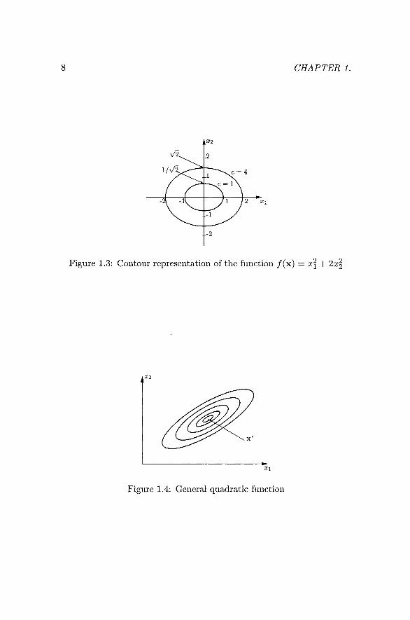
Figure 1.3 depicts the contour representation for the example / (x ) =

In three dimensions (n = 3), the contours are surfaces of constant func­tion value. In more than three dimensions (n > 3) the contours are, of course, impossible to visualize. Nevertheless, the contour representation in two-dimensional space will he used throughout the discussion of opti­mization techniques to help visualize the various optimization concepts.

Other examples of 2-dimensional objective function contours are shown in Figures 1.4 to 1.6.

CHAPTER 1.

Figure 1.3: Contour representation of the function / (x) = x\-\- 2x2

Figure 1.4: General quadratic function

INTRODUCTION

-2 -1.5 -1 -0.5 0 0.5 1 1.5 2

Figure 1.5: The 'banana' function / (x) = 10(a:2 - Xif + (1 — xi)

10 12 14

Figure 1.6: Potential energy function of a spring-force system (Vander-plaats, 1998)

10 CHAPTER 1.

15 10 5 9M = 0 -5 -10 -15

Boundary of feasible region

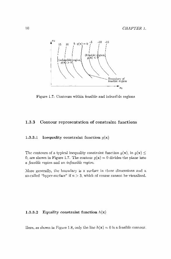
Figure 1.7: Contours within feasible and infeasible regions

1.3.3 Contour representat ion of constraint functions

1.3.3.1 Inequality constraint function ^(x)

The contours of a typical inequality constraint function g{'x.)^ in ^(x) < 0, are shown in Figure 1.7. The contour ^(x) = 0 divides the plane into a feasible region and an infeasible region.

More generally, the boundary is a surface in three dimensions and a so-called "hyper-surface" if n > 3, which of course cannot be visualised.

1.3.3.2 Equality constraint function /i(x)

Here, as shown in Figure 1.8, only the hne ^(x) = 0 is a feasible contour.

INTRODUCTION 11

15 10 5 ^(x) = 0 -5 -10 -15

Feasible contour (more generally a feasible surface)

XI

Figure 1.8: Feasible contour of equality constraint

/ = 2g ^(x) = 0

unconstrained minimum

x * ; / ( x * ) = 12 (constrained minimum)

^ ö ( x ) < 0 y ^ (feasible region)

^ (x ) > 0 (infeasible region)

Figure 1.9: Contour representation of inequality constrained problem

1.3.4 Contour representations of constrained optimiza­tion problems

1.3.4.1 Representation of inequality constrained problem

Figure 1.9 graphically depicts the inequality constrained problem:

min/(x)

such that ^(x) < 0.

12 CHAPTER 1.

/ = 20

unconstrained minimum

(feasible line (surface)) /i(x) = 0

x * ; / ( x * ) = 12 (constrained minimum)

A(x) < 0 (infeasible region)

( x ) > 0 (infeasible region)

Figure 1.10: Contour representation of equality constrained problem

T l-x

0 V

Figure 1.11: Wire divided into two pieces with xi = x and X2 = 1 — x

1.3.4.2 Representation of equality constrained problem

Figure 1.10 graphically depicts the equality constrained problem:

min/(x)

such that h{x.) — 0.

1.3.5 Simple example illustrating the formulation and so­lution of an optimization problem

Problem: A length of wire 1 meter long is to be divided into two pieces, one in a circular shape and the other into a square as shown in Figure 1.11. What must the individual lengths be so that the total area is a

mmimum (

Formulation 1

INTRODUCTION 13

Set length of first piece = x, then the area is given by f{x) — Trr -f 6 . Since r = ^ and b = ^ ^ it follows that

/W-^h-^ x'\ (1 - x)

47rV 16 '

The problem therefore reduces to an unconstrained minimization prob­lem:

minimize/(x) = 0.1421x^ - 0.125a; + 0.0625.

Solution of Formulation 1

The function f{x) is quadratic, therefore an analytical solution is given h_

2a

-0.125 0.4398 m,

by the formula ^* = —^ (a > 0):

2(0.1421)

and 1-x* = 0.5602 m with /(x*) = 0.0350 m^

Formulation 2

Divide the wire into respective lengths xi and X2 {xi -i- X2 = 1). The area is now given by

/ (x) =7rr^ + b'^ = 7T (-^^ + ( ^ ) ^ = 0.0796X? + 0.0625^2.

Here the problem reduces to an equality constrained problem:

minimize / (x) = 0.0796a;? + 0.0625a;^

such that /i(x) = xi + a;2 — 1 = 0.

Solution of Formulation 2

This constrained formulated problem is more difficult to solve. The closed-form analytical solution is not obvious and special constrained optimization techniques, such as the method of Lagrange multipliers to be discussed later, must be apphed to solve the constrained problem analytically. The graphical solution is sketched in Figure 1.12.

14 CHAPTER 1.

= (0.4398,0.5602)

1 + X2 = 1

,/ = 0.0350

Figure 1.12: Graphical solution of Formulation 2

1.3.6 Maximizat ion

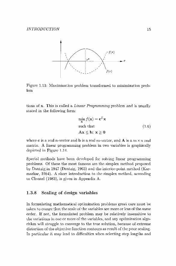
The maximization problem: max/(x) can be cast in the standard form X

(1.1) by observing that max/(x) = — mini—/(x)} as shown in Figure X X

1.13. Therefore in applying a minimization algorithm set F{x.) = —/(x).

Also if the inequality constraints are given in the non-standard form: 5'j(x) > 0, then set ^j(x) = —gj{x.). In standard form the problem then becomes:

minimize F(x) such that ^^(x) < 0.

Once the minimizer x* is obtained, the maximum value of the original maximization problem is given by — F(x*).

1.3.7 The special case of Linear Programming

A very important special class of the general optimization problem arises when both the objective function and all the constraints are linear func-

INTRODUCTION 15

i I

^^-~ .- ^ /w

Figure 1.13: Maximization problem transformed to minimization prob­lem

tions of X. This is called a Linear Programming problem and is usually stated in the following form:

min/(x) = c X

such that

Ax < b; X > 0

(1.6)

where c is a real n-vector and b is a real m-vector, and A is a m x n real matrix. A linear programming problem in two variables is graphically depicted in Figure 1.14.

Special methods have been developed for solving linear programming problems. Of these the most famous are the simplex method proposed by Dantzig in 1947 (Dantzig, 1963) and the interior-point method (Kar-markar, 1984). A short introduction to the simplex method, according to Chvatel (1983), is given in Appendix A.

1.3.8 Scaling of design variables

In formulating mathematical optimization problems great care must be taken to ensure that the scale of the variables are more or less of the same order. If not, the formulated problem may be relatively insensitive to the variations in one or more of the variables, and any optimization algo­rithm will struggle to converge to the true solution, because of extreme distortion of the objective function contours as result of the poor scaling. In particular it may lead to difficulties when selecting step lengths and

16 CHAPTER 1.

X2

y^ \ feasible region

\ \

direction of \ increase in ' y

\ \ y ^

\ \ \ J^C*

/ \

\

linear coi

Figure 1.14: Graphical representation of a two-dimensional linear pro­gramming problem

calculating numerical gradients. Scahng difficulties often occur where the variables are of different dimension and expressed in different units. Hence it is good practice, if the variable ranges are very large, to scale the variables so that all the variables will be dimensionless and vary between 0 and 1 approximately. For scaling the variables, it is necessary to establish an approximate range for each of the variables. For this, take some estimates (based on judgement and experience) for the lower and upper limits. The values of the bounds are not critical. Another related matter is the scaling or normalization of constraint functions. This becomes necessary whenever the values of the constraint functions differ by large magnitudes.

1.4 Further mathematical prerequisites

1.4.1 Convexity

A line through the points x^ and x^ in M^ is the set

L = {xlx = x^ + A(x2 - x^), for all A G (1.7)

INTRODUCTION 17

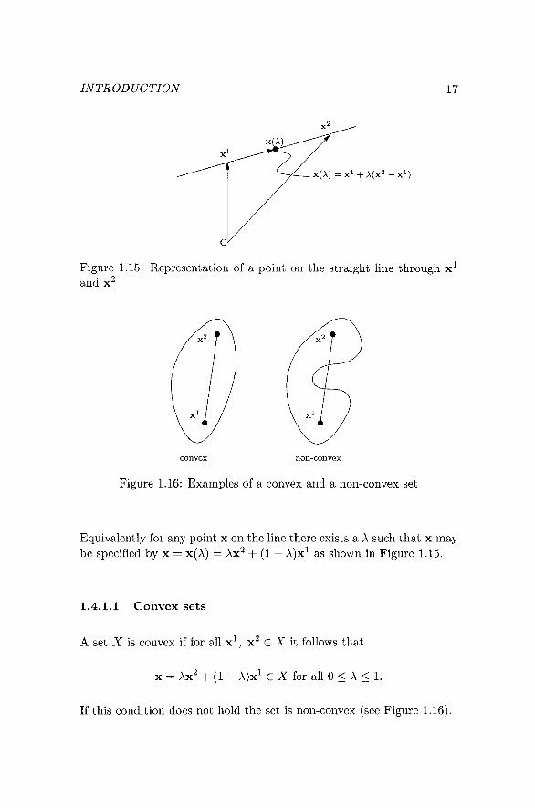
Figure 1.15: Representation of a point on the straight Hne through x- and x^

non-convex

Figure 1.16: Examples of a convex and a non-convex set

Equivalently for any point x on the line there exists a A such that x may be specified by x = x(A) = Ax^ + (1 ~ ^)^^ ^s shown in Figure 1.15.

1.4.1.1 Convex sets

A set X is convex if for all x \ x ^ G X it follows that

X = Ax^ -f- (1 - A)x^ G X for all 0 < A < 1.

If this condition does not hold the set is non-convex (see Figure 1.16).

18 CHAPTER 1.

1.4.1.2 Convex functions

Given two points x^ and x^ in R' , then any point x on the straight line connecting them (see Figure 1.15) is given by

X = x(A) = x^ + A(x2 - x^), 0 < A < 1. (1.8)

A function / (x) is a convex function over a convex set X if for all x^, x^ \nX and for all A G [0,1]:

/(Ax2 + (1 - A)xi) < A/(x2) + (1 - A)/(xi). (1.9)

The function is strictly convex if < applies. Concave functions are sim­ilarly defined.

Consider again the line connecting X"* and x^. Along this line, the func­tion / (x) is a function of the single variable A:

F(A) ^ /(x(A)) = /(x^ + A(x2 - x^)). (1.10)

This is equivalent to F(A) = /(Ax^ + (1 - A)x^), with F(0) = /(x^) and F( l ) = / (x^). Therefore (1.9) may be written as

F{\) < XF{1) + (1 - A)F(O) = Fint

where Fint is the linearly interpolated value of F at A as shown in Figure 1.17.

Graphically / (x) is convex over the convex set X if F(A) has the convex form shown in Figure 1.17 for any two points x^ and x^ in X.

1.4.2 Gradient vector of /(x)

For a function / (x) G C^ there exists, at any point x a vector of first order partial derivatives, or gradient vector:

ox I

V/(x) = 3X2

(^)

OXn

g(x). (1.11)

INTRODUCTION 19

Figure 1.17: Convex form of F{X)

Figure 1.18: Directions of the gradient vector

It can easily be shown that if the function / (x) is smooth, then at the point x the gradient vector V / ( x ) (also often denoted by g(x)) is always perpendicular to the contours (or surfaces of constant function value) and is in the direction of maximum increase of / (x ) , as depicted in Figure 1.18.

20 CHAPTER L

1.4.3 Hess ian matrix of / ( x )

If / (x) is twice continuously differentiable then at the point x there exists a matrix of second order partial derivatives or Hessian matrix:

H(x) \ dxidxj J dxidxj

(x) j> = VV(x

(x)

(x)

(x)

9x19x2 (x)

9xri9xi

Clearly H(x) is a n x n symmetrical matrix.

(1.12)

1.4.3.1 Test for convexity of / (x)

If / (x ) G C^ is defined over a convex set X, then it can be shown (see Theorem 6.1.3 in Chapter 6) that if H(x) is positive-definite for all X G X, then / (x) is strictly convex over X.

To test for convexity, i.e. to determine whether H(x) is positive-definite or not, apply Sylvester's Theorem or any other suitable numerical method (Fletcher, 1987).

1.4.4 T h e quadratic function in

The quadratic function in n variables may be written as

/ (x) = ^x^Ax + b^x + c (1.13)

where c G R, b is a real n-vector and A is a n x n real matrix that can be chosen in a non-unique manner. It is usually chosen symmetrical in which case it follows that

V / ( x ) = Ax + b; H ( x ) - A . (1.14)

INTRODUCTION 21

The function / (x) is called positive-definite if A is positive-definite since, by the test in 1.4.3.1, a function / (x) is convex if H(x) is positive-definite.

1.4.5 The directional derivative of / ( x ) in the direct ion u

It is usually assumed that ||u|| — 1. Consider the diff'erential:

df = ^dxi + . . . + ^dxn = V^/ (x)dx . (1.15)

A point X on the line through x' in the direction u is given by x = x(A) = x' + Au, and for a small change dA in A, dx = udA. Along this line F{X) — / ( x ' + Au) and the differential at any point x on the given line in the direction u is therefore given by dF = df = V^/(x)udA. It follows that the directional derivative at x in the direction u is

dF{X) df{K)

dX dX V V ( x ) u . (1.16)

1.5 Unconstrained minimization

In considering the unconstrained problem: min/ (x) , x G X C R^, the X

following questions arise:

(i) what are the conditions for a minimum to exist,

(ii) is the minimum unique,

(iii) are there any relative minima?

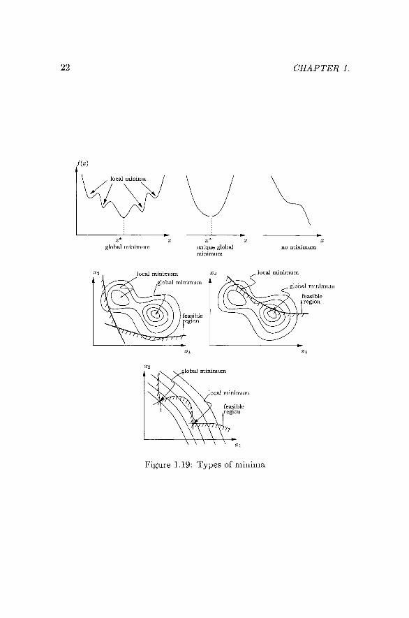
Figure 1.19 (after Farkas and Jarmai, 1997) depicts different types of minima that may arise for functions of a single variable, and for functions of two variables in the presence of equality constraints. Intuitively, with reference to Figure 1.19, one feels that a general function may have a single unique global minimum, or it may have more than one local minimum. The function may indeed have no local minimum at all, and in two dimensions the possibihty of saddle points also comes to mind.

22 CHAPTER 1.

fix)

global minimum unique global minimum

no m m i m u m

local min imum

global min imum

Figure 1.19: Types of minima

INTRODUCTION 23

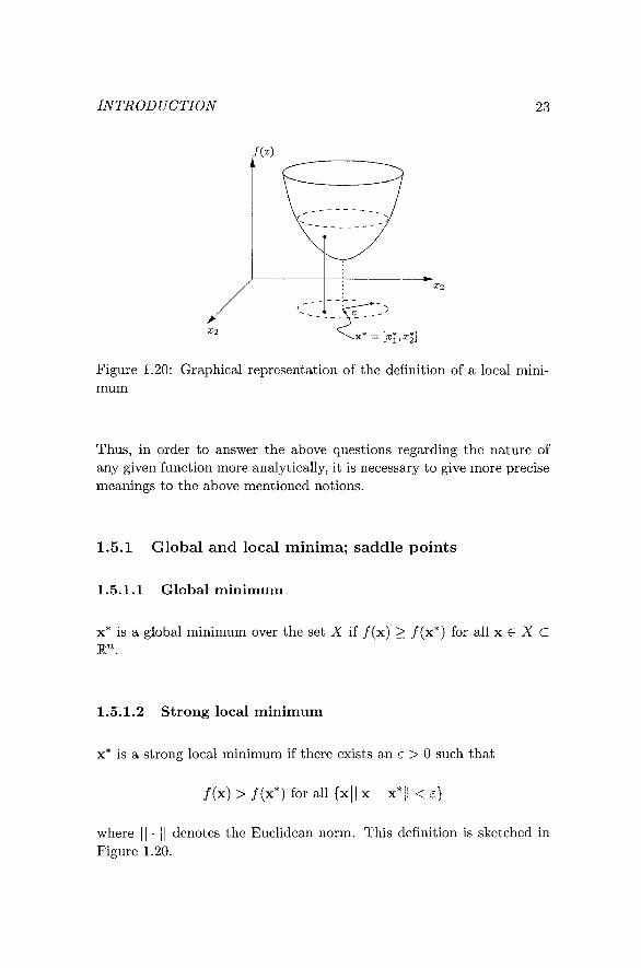
Figure 1.20: Graphical representation of the definition of a local mini­mum

Thus, in order to answer the above questions regarding the nature of any given function more analytically, it is necessary to give more precise meanings to the above mentioned notions.

1.5.1 Global and local minima; saddle points

1.5.1.1 Global minimum

X* is a global minimum over the set X if / (x) > /(x*) for all x G X C

1.5.1.2 Strong local minimum

X* is a strong local minimum if there exists an ^ > 0 such that

where || Figure 1.20.

/ ( x ) > / ( x * ) f o r a l l { x | | | x - x * | | < e }

denotes the Euclidean norm. This definition is sketched in

24 CHAPTER 1.

1.5.1.3 Test for unique local global minimum

It can be shown (see Theorems 6.1.4 and 6.1.5 in Chapter 6) that if / (x) is strictly convex over X, then a strong local minimum is also the global minimum.

The global minimizer can be difficult to find since the knowledge of / (x ) is usually only local. Most minimization methods seek only a local min­imum. An approximation to the global minimum is obtained in practice by the multi-start application of a local minimizer from randomly se­lected different starting points in X. The lowest value obtained after a sufficient number of trials is then taken as a good approximation to the global solution (see Snyman and Fatti, 1987; Groenwold and Snyman, 2002). If, however, it is known that the function is strictly convex over X, then only one trial is sufficient since only one local minimum, the global minimum, exists.

1.5.1.4 Saddle points

/ (x) has a saddle point at x — if there exists an £ > 0 such that

for all X, ||x - xO|| < s and all y, ||y - yO|| < e: / (x .y») < /(xO.yO) < /(xO,y).

A contour representation of a saddle point in two dimensions is given in Figure 1.21.

1.5.2 Local characterization of the behaviour of a multi-variable function

It is assumed here that / (x) is a smooth function, i.e., that it is a twice continuously differentiable function (/(x) G C^). Consider again the hne x = x(A) = x' + Au through the point x' in the direction u.

Along this hne a single variable function F{\) may be defined:

F(A) = /(x(A)) = / ( x ' + Au).

INTRODUCTION 25

Figure 1.21: Contour representation of saddle point

It follows from (1.16) that

dF{X) ^/(x(A))

dX dX = V^/(x(A))u = ^(x(A)) = G(A)

which is also a single variable function of A along the line x = x(A) x' + Au.

Thus similarly it follows that

d^F{X) dG{X) dg{x{X)) dA2 dX dX

= V^5(x(A))u

= V ^ (V^/(x(A))u) u

= u^H(x(A))u.

Summarising: the first and second order derivatives of -F'(A) with respect to A at any point x = x(A) on any line (any u) through x' is given by

dFjX)

dX

d^FjX) dX^

= V^/(x(A))u,

u^H(x(A))u

(1.17)

(1.18)

26 CHAPTER 1.

where x(A) - x' + Au and F{X) = /(x(A)) = / ( x ' + Au).

These results may be used to obtain Taylor's expansion for a multi-variable function. Consider again the single variable function F{X) de­fined on the fine through x' in the direction u by F{X) = / ( x ' + Au). It is known that the Taylor expansion of F{X) about 0 is given by

F(A) = F(0) + AF'(O) + IX^F'^Q) + . . . (1.19)

With F(0) = / (x ' ) , and substituting expressions (1.17) and (1.18) for respectively F'(A) and F''{X) at A = 0 into (1.19) gives

F(A) - / ( x ' + Au) = /(xO + V ^ / ( X O A U + iAu^H(xOAu - } - . . .

Setting J = Au in the above gives the expansion:

/ ( x ' + S) = /(x') + V^fiK')6 + lS^H{x')S +... (1.20)

Since the above applies for any line (any u) through x', it represents the general Taylor expansion for a multi-variable function about x'. If / (x) is fully continuously diff'erentiable in the neighbourhood of x ' it can be shown that the truncated second order Taylor expansion for a multi-variable function is given by

/ ( x ' + (5) = / (x ' ) + V^/(x')(5 + ^5^H(x' + OS)S (1.21)

for some 6 G [0,1]. This expression is important in the analysis of the behaviour of a multi-variable function at any given point x'.

1.5.3 Necessary and sufficient conditions for a s trong lo­cal minimum at x*

In particular, consider x' = x* a strong local minimizer. Then for any line (any u) through x' the behaviour of F{X) in a neighbourhood of x* is as shown in Figure 1.22, with minimum at at A == 0.

Clearly, a necessary first order condition that must apply at x* (corre­sponding to A = 0) is that

dF{0) _ ^T dX

V V ( x * ) u = 0, f o r a l l u / 0 . (1.22)

INTRODUCTION 27

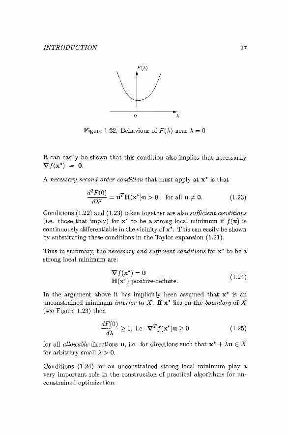
F(A)

Figure 1.22: Behaviour of F{X) near A = 0

It can easily be shown that this condition also implies that necessarily V/(x*) = 0.

A necessary second order condition that must apply at x* is that

^2^(0)

d\^ = u ' H(x*)u > 0, for all u 7 0. (1.23)

Conditions (1.22) and (1.23) taken together are also sufficient conditions (i.e. those that imply) for x* to be a strong local minimum if / (x ) is continuously differentiable in the vicinity of x*. This can easily be shown by substituting these conditions in the Taylor expansion (1.21).

Thus in summary, the necessary and sufficient conditions for x* to be a strong local minimum are:

V/(x*) = 0 H(x*) positive-definite.

In the argument above it has implicitly been assumed that x* is an unconstrained minimum interior to X. If x* lies on the boundary of X (see Figure 1.23) then

^ > 0 , i.e. V ^ / ( x > > 0 (1.25)

for all allowable directions u, i.e. for directions such that x* + Au G X for arbitrary small A > 0.

Conditions (1.24) for an unconstrained strong local minimum play a very important role in the construction of practical algorithms for un­constrained optimization.

28 CHAPTER 1.

Fix)

Figure 1.23: Behaviour of F{X) for all allowable directions of u

1.5.3.1 Application to the quadratic function

Consider the quadratic function:

/ (x) - i x ^ A x + b^x + c.

In this case the first order necessary condition for a minimum implies that

V / ( x ) = Ax + b = 0.

Therefore a candidate solution point is

X* = - A - ^ b . (1.26)

If the second order necessary condition also apphes, i.e. if A is positive-definite, then X* is a unique minimizer.

1.5.4 General indirect m e t h o d for comput ing x*

The general indirect method for determining x* is to solve the system of equations V / ( x ) = 0 (corresponding to the first order necessary condition in(1.24)) by some numerical method, to yield all stationary points. An obvious method for doing this is Newton's method. Since in general the system will be non-hnear, multiple stationary points are possible. These stationary points must then be further analysed in order to determine whether or not they are local minima.

INTRODUCTION 29

1.5.4.1 Solution by Newton's method

Assume x* is a local minimum and x* an approximate solution, with associated unknown error ö such that x* — -x} -\- 8. Then by applying Taylor's theorem and the first order necessary condition for a minimum at X* it follows that

0 = V/(x*) - V/(x^ + 5) - V/(x^) + H(x^)(5 + 0\\ö\\\

If x^ is a good approximation then J = A, the solution of the linear system H(x*)A + V/(x*) = 0, obtained by ignoring the second order term in 6 above. A better approximation is therefore expected to be x^+^ = X* + A which leads to the Newton iterative scheme: Given an initial approximation x^, compute

x^+i :=: x^ _ H-Hx^)V/(x^) (1.27)

for i = 0, 1, 2, . . . Hopefully lim x = x*.

1.5.4.2 Example of Newton's method applied to a quadratic problem

Consider the unconstrained problem:

minimize / (x) — ^x"^ Ax + b"^x + c.

In this case the first iteration in (1.27) yields

x^ = x° - A-i (Axö + b) = x^ - x^ - A-^b - - A - ^ b

i.e. x^ = X* = —A~- b in a single step (see (1.26)). This is to be expected since in this case no approximation is involved and thus A — 5.

1.5.4.3 Difficulties with Newton's method

Unfortunately, in spite of the attractive features of the Newton method, such as being quadratically convergent near the solution, the basic New­ton method as described above does not always perform satisfactorily. The main difficulties are:

30 CHAPTER 1.

y = <t>{x)

0 X* x^ X 0 X* x^ X

Figure 1.24: Graphical representation of Newton's iterative scheme for a single variable

(i) the method is not always convergent, even if x^ is close to x*, and

(ii) the method requires the computation of the Hessian matrix at each iteration.

The first of these difficulties may be illustrated by considering Newton's method applied to the one-dimensional problem: solve f\x) = 0. In this case the iterative scheme is

x^+i =x'- 4 Ö = (t>{x'), for z = 0, 1, 2, nx^)

(1.28)

and the solution corresponds to the fixed point x* where x* = 0(x*). Unfortunately in some cases, unless x^ is chosen to be exactly equal to X*, convergence will not necessarily occur. In fact, convergence is de­pendent on the nature of the fixed point function (/)(a;) in the vicinity of X , as shown for two different 0 functions in Figure 1.24. With ref­erence to the graphs Newton's method is: y = </>(a;*), x " ^ = y'^ for 2 = 0, 1, 2, Clearly in the one case where |0'(x)| < 1 convergence occurs, but in the other case where |0'(x)| > 1 the scheme diverges.

In more dimensions the situation may be even more complicated. In addition, for a large number of variables, difficulty (ii) mentioned above becomes serious in that the computation of the Hessian matrix repre­sents a major task. If the Hessian is not available in analytical form, use can be made of automatic differentiation techniques to compute it,

INTRODUCTION 31

or it can be estimated by means of finite differences. It should also be noted that in computing the Newton step in (1.27) a n x n linear system must be solved. This represents further computational effort. There­fore in practice the simple basic Newton method is not recommended. To avoid the convergence difficulty use is made of a modified Newton method, in which a more direct search procedure is employed in the direction of the Newton step, so as to ensure descent to the minimum X*. The difficulty associated with the computation of the Hessian is addressed in practice through the systematic update, from iteration to iteration, of an approximation to the Hessian matrix. These improve­ments to the basic Newton method are dealt with in greater detail in the next chapter.

1.6 Exercises

1.6.1 Sketch the graphical solution to the following problem:

minx/(x) = ( x i - 2 ) 2 + (x2-2)2

such that xi + 2x2 = 4; xi > 0; X2 > 0.

In particular indicate the feasible region: F = {{xi,X2)\xi -{-2x2 = 4;

xi > 0;X2 > 0} and the solution point x*.

1.6.2 Show that x^ is a convex function.

1.6.3 Show that the sum of convex functions is also convex.

1.6.4 Determine the gradient vector and Hessian of the Rosenbrock func­tion:

/(X) = 100(x2-x2)2 + ( l _ x i ) 2 .

1.6.5 Write the quadratic function / (x) = x^ -f 2xiX2 + Sx^ in the stan­dard matrix-vector notation. Is / (x) positive-definite?

1.6.6 Write each of the following objective functions in standard form:

/ (x) = ^x^Ax + b^x + c.

(i) / (x ) = x?4-2xiX24-4xiX3+3x2+2x2X3+5x3+4xi-2x2+3x3.

32 CHAPTER 1.

(ii) / (x ) = 5x^ + 12x1X2 - 16x1X3 + 10x| - 26x2x3 + 17x| - 2xi -4x2 - 62:3.

(iii) / (x ) = x\ — 4xiX2 -f 6x1X3 4- 5x1 — IOX2X3 + 8x3.

1.6.7 Determine the definiteness of the following quadratic form: /(x) = x\ — 4xiX2 -f 6x1X3 + 5X2 - 10X2X3 + 8X3.

Chapter 2

LINE SEARCH DESCENT METHODS FOR UNCONSTRAINED MINIMIZATION

2.1 General line search descent algorithm for unconstrained minimization

Over the last 40 years many powerful direct search algorithms have been developed for the unconstrained minimization of general functions. These algorithms require an initial estimate to the optimum point, de­noted by x^. With this estimate as starting point, the algorithm gen­erates a sequence of estimates x^, x^, x^, . . . , by successively searching directly from each point in a direction of descent to determine the next point. The process is terminated if either no further progress is made, or if a point x^ is reached (for smooth functions) at which the first necessary condition in (1.24), i.e. V / ( x ) = 0 is sufficiently accurately satisfied, in which case x* = x^. It is usually, although not always, required that the function value at the new iterate x*" ^ be lower than that at x \

34 CHAPTER 2.

An important sub-class of direct search methods, specifically suitable for smooth functions, are the so-called line search descent methods. Basic to these methods is the selection of a descent direction u*" ^ at each iterate X* that ensures descent at x* in the direction u^+^, i.e. it is required that the directional derivative in the direction u*" ^ be negative:

d/(x^) VV(x')u^ '^ ' < 0 . (2.1)

d\

The general structure of such descent methods is given below.

2.1.1 General s tructure of a line search descent m e t h o d

1. Given starting point x^ and positive tolerances £i, £2 and £3, set i = 1.

2. Select a descent direction u^ (see descent condition (2.1).

3. Perform a one-dimensional line search in direction u^: i.e.

minF(A) = min/(x^-^ + Au^)

to give minimizer A .

4. Set x^ = x^-^ + A^u^

5. Test for convergence:

if ||x^ - x^-i|| < £1, or II V/(xO| | < ^2, or |/(xO - /(x^"^)! < ^3, then STOP and x* ^ xS

else go to Step 6.

6. Set i = i + 1 and go to Step 2.

In testing for termination in step 5, a combination of the stated termi­nation criteria may be used, i.e. instead of or, and may be specified. The structure of the above descent algorithm is depicted in Figure 2.1.

Different descent methods, within the above sub-class, differ according to the way in which the descent directions u^ are chosen. Another impor­tant consideration is the method by means of which the one-dimensional line search is performed.

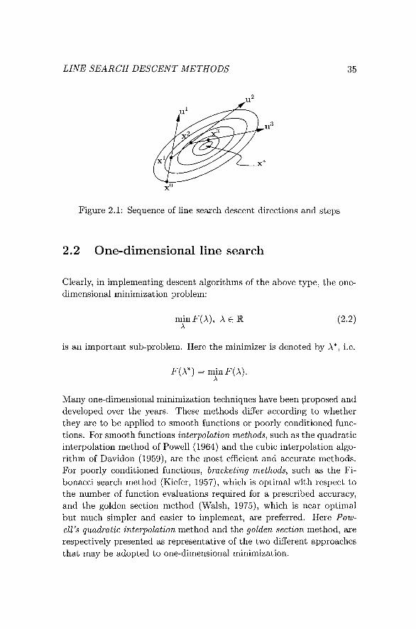
LINE SEARCH DESCENT METHODS 35

Figure 2.1: Sequence of line search descent directions and steps

2.2 One-dimensional line search

Clearly, in implementing descent algorithms of the above type, the one-dimensional minimization problem:

minF(A), A G R (2.2)

is an important sub-problem. Here the minimizer is denoted by A*, i.e.

F(A*)=:minF(A). A

Many one-dimensional minimization techniques have been proposed and developed over the years. These methods differ according to whether they are to be applied to smooth functions or poorly conditioned func­tions. For smooth functions interpolation methods, such as the quadratic interpolation method of Powell (1964) and the cubic interpolation algo­rithm of Davidon (1959), are the most efficient and accurate methods. For poorly conditioned functions, bracketing methods, such as the Fi­bonacci search method (Kiefer, 1957), which is optimal with respect to the number of function evaluations required for a prescribed accuracy, and the golden section method (Walsh, 1975), which is near optimal but much simpler and easier to implement, are preferred. Here Pow­ell's quadratic interpolation method and the golden section method, are respectively presented as representative of the two different approaches that may be adopted to one-dimensional minimization.

36 CHAPTER 2.

a Al A* A2 h

Figure 2.2: Unimodal function F[\) over interval [a, h]

2.2.1 Golden sect ion m e t h o d

It is assumed that F{\) is unimodal ower the interval [a, 6], i.e. that it has a minimum A* within the interval and that F{\) is strictly descending for A < A* and strictly ascending for A > A*, as shown in Figure 2.2.

Note that if F{\) is unimodal over [a, h] with A* in [a, 6], then to deter­mine a sub-unimodal interval, at least two evaluations of F{\) in [a, h] must be made as indicated in Figure 2.2.

If F(A2) > i^(Ai) =^ new unimodal interval == [a, A2], and set 6 = A2 and select new A2; otherwise new unimodal interval = [Ai,6] and set a = \i and select new Ai.

Thus, the unimodal interval may successively be reduced by inspecting values of F{Xi) and F{X2) at interior points Ai and A2.

The question arises: How can Ai and A2 be chosen in the most eco­nomic manner, i.e. such that a least number of function evaluations are required for a prescribed accuracy (i.e. for a specified uncertainty inter­val)? The most economic method is the Fibonacci search method. It is however a complicated method. A near optimum and more straightfor­ward method is the golden section method. This method is a limiting form of the Fibonacci search method. Use is made of the golden ratio r when selecting the values for Ai and A2 within the unimodal interval. The value of r corresponds to the positive root of the quadratic equation:

1 = 0, thus r = ^%^ - 0.618034. r'^ ^-r

LINE SEARCH DESCENT METHODS 37

Al — a + r^I/o A2 = a + TLQ

rLo r^Lo

Figure 2.3: Selection of interior points Ai and A2 for golden section search

The details of the selection procedure are as follows. Given initial uni-modal interval [a, &] of length LQ, then choose interior points Ai and A2 as shown in Figure 2.3.

Then, if F(Ai) > F(A2) =^ new [a,b] = [Ai,6] with new interval length Li = rl/o, and

if F{X2) > F{Xi) => new [a, b] = [a, A2] also with Li = rLo-

The detailed formal algorithm is stated below.

2.2.1.1 Basic golden section algorithm

Given interval [a, b] and prescribed accuracy e; then set i = 0; LQ = b—a, and perform the following steps:

1. Set Al = a + r^Lo; A2 = a -f TLQ.

2. Compute F{\i) and -F(A2); set i = i -f 1.

3. / /F(Ai) >F(A2) then

set a = Ai; Ai = A2; Li = {b — a); and A2 = a + rLi^

else

set b = A2; A2 = Ai; Li = {b — a); and Xi = a + r^Li.

4. If Li < e then

set A = —-—; compute F(A*) and STOP,

else go to Step 2.

38 CHAPTER 2.

P2(A) F{X)

A0A1A2 \m A*

Figure 2.4: Approximate minimum Am via quadratic interpolation

2.2.2 Powell 's quadratic interpolat ion algori thm

In Powell's method successive quadratic interpolation curves are fitted to function data giving a sequence of approximations to the minimum point A*.

With reference to Figure 2.4, the basic idea is the following. Given three data points {(A^,F(Ai)), i = 1,2,3}, then the interpolating quadratic polynomial through these points P2W is given by

P2(A) = F(Ao) + F[Ao, Ai](A - AQ) + F[Ao, Ai, Aa^A - Ao)(A - Ai) (2.3)

where F[ , ] and F[ , , ] respectively denote the first order and second order divided differences.

The turning point of p2(A) occurs where the slope is zero, i.e. where

^ = F[Ao, Al] + 2AF[Ao, Ai, A2] - F[Ao, Ai, A2](Ao -f Ai) = 0

which gives the turning point Xm as

F[Ao,Ai,A2](Ao + Ai)-i^[Ao,Ai] Xr]

2F[Ao,Ai,A2] ^A* (2.4)

with the further condition that for a minimum the second derivative must be non-negative, i.e. F[Ao,Ai,A2] > 0.

The detailed formal algorithm is as follows.

LINE SEARCH DESCENT METHODS 39

2.2.2.1 Powell's interpolation algorithm

Given starting point AQ, stepsize /i, tolerance e and maximum stepsize H\ perform following steps:

1. Compute F(Ao) and F(Ao + h).

2. IfF{Xo) < F{Xo + h) evaluate F(Ao - h),

else evaluate F(Ao + 2/i). (The three initial values of A so chosen constitute the initial set (Ao,Ai,A2) with corresponding function values F{Xi), 2 = 0,1,2.)

3. Compute turning point Xm by formula (2.4) and test for minimum or maximum.

4. If Xm a minimum point and \Xm — Xn\ > H^ where A^ is the nearest point to Xm, then discard the point furthest from Xm and take a step of size H from the point with lowest value in direction of descent, and go to Step 3;

^/Am a maximum point, then discard point nearest A^ and take a step of size H from the point with lowest value in the direction of descent and go to Step 3;

else continue.

5. If\Xm -Xn\<e then F(A*) ^ min[F(A^),F(An)] and STOP,

else continue.

6. Discard point with highest F value and replace it by A T ; go to Step 3

Note: It is always safer to compute the next turning point by interpola­tion rather than by extrapolation. Therefore in Step 6: if the maximum value of F corresponds to a point which lies alone on one side of Xm, then rather discard the point with highest value on the other side of A,^.

2.2.3 Exercises

Apply the golden section method and Powell's method to the problems below. Compare their respective performances with regard to the num-

40 CHAPTER 2.

her of function evaluation required to attain the prescribed accuracies.

(i) minimize F(A) = A + 2e"'^ over [0,2] with e = 0.01.

(ii) maximize F{X) = A cos A over [0,7r/2] with s — 0.001.

(iii) minimize F(A) = 4 ( A - 7 ) / ( A 2 + A - 2 ) over [-1.9; 0.9] by performing only 10 function evaluations.

(iv) minimize F(A) = A - 20A^ + 0.1 A over [0; 20] with e - 10"^.

2.3 First order line search descent methods

Line search descent methods (see Section 2.1.1), that use the gradient vector V / ( x ) to determine the search direction for each iteration, are called first order methods because they employ first order partial deriva­tives of / (x ) to compute the search direction at the current iterate. The simplest and most famous of these methods is the method of steepest descent, first proposed by Cauchy in 1847.

2.3.1 The method of steepest descent

In this method the direction of steepest descent is used as the search direction in the line search descent algorithm given in section 2.1.1. The expression for the direction of steepest descent is derived below.

2.3.1.1 The direction of steepest descent

At x' we seek the unit vector u such that for F{X) — / ( x ' + Au), the directional derivative

df{^') dX

dF{0) _ ^r dX

V ^ / ( x ' ) u

assumes a minimum value with respect to all possible choices for the unit vector u at x' (see Figure 2.5).

LINE SEARCH DESCENT METHODS 41

Figure 2.5: Search direction u relative to gradient vector at x '

By Schwartz's inequality:

V^ / (xOu > - | |V/(x ') l i | |u | | - - | | V / ( x ' ) | | - least value.

-V/(xO Clearly for the particular choice u — the directional derivative

at x' is given by

Thus this particular choice for the unit vector corresponds to the direc­tion of steepest descent.

The search direction

is called the normalized steepest descent direction at x.

2.3.1.2 Steepest descent algori thm

Given x°, do for iteration i = 1, 2 , . . . until convergence:

• _ - V / ( x ^ - ^ )

' • ' ' ' ^ - | | V / ( x ^ - i ) | |

2. set x^ = x*~- + A u* where A is such that

F{Xi) - /(x^-^ + Xiu') = min/(x^-i + Au ) (line search). A

42 CHAPTER 2.

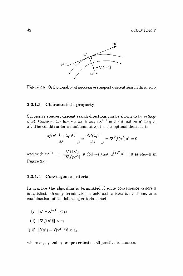
Figure 2.6: Orthogonality of successive steepest descent search directions

2.3.1.3 Characteristic property

Successive steepest descent search directions can be shown to be orthog­onal Consider the line search through x^~^ in the direction u* to give x \ The condition for a minimum at A , i.e. for optimal descent, is

4f (x^-i + A u ) d\

dF{Xi)

dX V^/(x^)u^ = 0

u

V f fxM T and with u " ^ = — , ,^ ^, .,,, it follows that u*" ^ u* = 0 as shown in l|V/(xO|| Figure 2.6.

2.3.1.4 Convergence criteria

In practice the algorithm is terminated if some convergence criterion is satisfied. Usually termination is enforced at iteration i if one, or a combination, of the following criteria is met:

(i) | | x ^ - x ^ - i | | < £ i

(ii) | |V / (xO | |<52

(iii) | / ( X 0 - / ( X - I ) | < e 3 .

where si , £2 and £3 are prescribed small positive tolerances.

LINE SEARCH DESCENT METHODS 43

10- 10- 10-

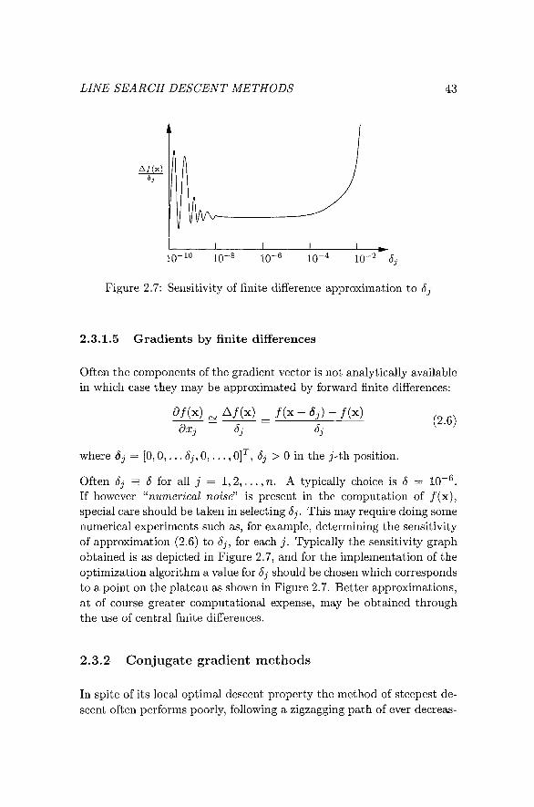
Figure 2.7: Sensitivity of finite difference approximation to 5j

2.3.1.5 Gradients by finite differences

Often the components of the gradient vector is not analytically available in which case they may be approximated by forward finite differences:

ö/(x) ^ A/(x) _ / ( x + g , ) - / (x ) dxj Sj

(2.6)

where Sj = [0, 0 , . . . 5j, 0 , . . . , 0]-^, 6j > 0 in the j-th position.

Often Sj = S for all j = 1,2, . . . , n . A typically choice is J = 10~^. If however '^numerical noise^^ is present in the computation of / (x ) , special care should be taken in selecting öj. This may require doing some numerical experiments such as, for example, determining the sensitivity of approximation (2.6) to Jj, for each j . Typically the sensitivity graph obtained is as depicted in Figure 2.7, and for the implementation of the optimization algorithm a value for 5j should be chosen which corresponds to a point on the plateau as shown in Figure 2.7. Better approximations, at of course greater computational expense, may be obtained through the use of central finite differences.

2.3.2 Conjugate gradient m e t h o d s

In spite of its local optimal descent property the method of steepest de­scent often performs poorly, following a zigzagging path of ever decreas-

44 CHAPTER 2.

Figure 2.8: Orthogonal zigzagging behaviour of the steepest descent method

ing steps. This results in slow convergence and becomes extreme when the problem is poorly scaled, i.e. when the contours are extremely elon­gated. This poor performance is mainly due to the fact that the method enforces successive orthogonal search directions (see Section 2.3.1.3) as shown in Figure 2.8. Although, from a theoretical point of view, the method can be proved to be convergent, in practice the method may not effectively converge within a finite number of steps. Depending on the starting point this poor convergence also occurs when applying the method to positive-definite quadratic functions.

There is, however, a class of first order fine search descent methods, known as conjugate gradient methods^ for which it can be proved that whatever the scaling, a method from this class will converge exactly in a finite number of iterations when applied to a positive-definite quadratic function, i.e. to a function of the form

/ (x) = ^x^Ax + b^x + c (2.7)

where c G M, b is a real n-vector and A is a positive-definite n x n real symmetric matrix. Methods that have this property of quadratic termination are highly rated, because they are expected to also perform well on other non-quadratic functions in the neighbourhood of a local minimum. This is so, because by the Taylor expansion (1.21), it can be seen that many general differentiable functions approximate the form (2.7) near a local minimum.

LINE SEARCH DESCENT METHODS 45

2.3.2.1 Mutually conjugate directions

Two vectors u, v ^ 0 are defined to be orthogonal if the scalar product u-^v = (u, v) = 0. The concept of mutual conjugacy may be defined in a similar manner. Two vectors u, v ^ 0, are defined to be mutually conjugate with respect to the matrix A in (2.7) if u-^Av = (u, Av) = 0. Note that A is a positive definite symmetric matrix.

It can also be shown (see Theorem 6.5.1 in Chapter 6) that if the set of vectors u ^ z = l , 2 , . . . , n are mutually conjugate^ then they form a basis in R"", i.e. any x G M"' may be expressed as

= ^ W (2.8)

where

X

i=l

^^-(uSAuO* ^ ^ ^

2.3.2.2 Convergence theorem for mutually conjugate direc­tions

Suppose u% i = 1,2, . . . ,n are mutually conjugate with respect to positive-definite A, then the optimal line search descent method in Sec­tion 2.1.1, using u^ as search directions, converges to the unique mini­mum x* of / (x ) = ^x-^Ax + b^x + c in less than or equal to n steps.

Proof:

If x^ the starting point, then after i iterations:

x^ = x^-i + A u = x'-'^-{-Xi_iu'-^ + Xiu' = . . . i

= x° + 5]Afeu\ (2.10) k=l

The condition for optimal descent at iteration i is

dF{Xi) rf/(x^-i + Aiu') dX dX

= K,v/(x^-i + W ) ] = 0

= [u',V/(x^)] = 0

46 CHAPTER 2.

i.e.

0 = (u',Ax' + b)

= U \ A f x ' ' + ^ A f c u M + b j = K,AxO + b) + Ai(u',Au')

because u' , i = l , 2 , . . . , n are mutually conjugate, and thus

\i = -{u\ Ax° + b ) / ( u \ Au ' ) . (2.11)

Substituting (2.11) into (2.10) above gives

u%AxO)u^ ^ (uSA(A-ib))u^ ;: (u%Au^) ^ (u%Au^)

Now by utilizing (2.8) and (2.9) it follows that

x^ - x^ - x° - A-^b = - A - ^ b = X*.

The implication of the above theorem for the case n — 2 and where mutually conjugate line search directions u^ and u^ are used, is depicted in Figure 2.9.

2.3.2.3 Determination of mutually conjugate directions

How can mutually conjugate search directions be found? One way is to determine all the eigenvectors u \ i = 1,2,... ,n of A. For A positive-definite, all the eigenvectors are mutually orthogonal and since Au^ = jj^iU^ where ßi is the associated eigenvalue, it follows directly that for all i ^ j that (u \ Au-^) = (u\/XjU-^) = /ij(u^,u-^) = 0, i.e. the eigenvectors are mutually conjugate with respect to A. It is, however, not very practical to determine mutually conjugate directions by finding all the eigenvectors of A, since the latter task in itself represents a com­putational problem of magnitude equal to that of solving the original unconstrained optimization problem via any other numerical algorithm. An easier method for obtaining mutually conjugate directions, is by means of the Fletcher-Reeves formulae (Fletcher and Reeves, 1964).

LINE SEARCH DESCENT METHODS 47

Figure 2.9: Quadratic termination of the conjugate gradient method in two steps for the case n = 2

2.3.2.4 The Fletcher-Reeves directions

The Fletcher-Reeves directions u \ z = 1,2,... ,n, that are listed below, can be shown (see Theorem 6.5.3 in Chapter 6) to be mutually conjugate with respect to the matrix A in the expression for the quadratic function in (2.7) (for which V / ( x ) = Ax + b). The explicit directions are:

ui = -V/ (xO)

and for i = 1,2,. . . , n — 1

„i+i ^ - v / ( x ' ) + ßiu' (2.12)

where x* = x^ ^ + AiU% and A corresponds to the optimal descent step in iteration i, and

i|V/(xO|P Ä = (2.13)

| |V / (x - i ) | | 2 -

The Polak-Ribiere directions are obtained if, instead of using (2.13), ßi is computed using

ßi = (V/(x') - V/(x-^))^ V/(x»)

| |V/ (x- i ) i-l\\\2 (2.14)

I f / (x) is quadratic it can be shown (Fletcher, 1987) that (2.14) is equiv­alent to (2.13).

48 CHAPTER 2.

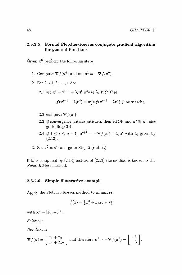
2.3.2.5 Formal Fletcher-Reeves conjugate gradient algorithm for general functions

Given x^ perform the following steps:

1. Compute V/ (x° ) and set u^ = -Vf{-xP).

2. For 2 = 1,2,... ,n do:

2.1 set X* = x*~- + A u* where A such that

/(x^-^ + XiM') = min/(x^-^ + Au ) (line search), A

2.2 compute V/ (xO,

2.3 i/convergence criteria satisfied, then STOP and x* ~ x \ else go to Step 2.4.

2Ä if 1 < i < n - 1, u^+i - - V / ( x O -f ßiu' with ßi given by (2.13).

3. Set x° = x^ and go to Step 2 (restart).

If ßi is computed by (2.14) instead of (2.13) the method is known as the Polak-Ribiere method.

2.3.2.6 Simple illustrative example

Apply the Fletcher-Reeves method to minimize

/ (x) = ^Xi + xia;2 + xl

withxö = [10,-5]^.

Solution:

Iteration 1:

V/(x) = Xi +X2 Xi + 2^2

and therefore u^ = —^/{x.^) = - 5

0

LINE SEARCH DESCENT METHODS 49

x = x° + Au 1 _ 10-5A - 5

and

F{\) = /(xO + Aui) = i(10 - 5A)2 + (10 - 5A)(-5) + 25.

For optimal descent

d\ v >' ~ d\

This gives Ai = 1, x^ =

Iteration 2:

U2 = - V / ( x l )

5(10 - 5A) + 25 = 0 (line search).

and V / ( x i ) = 5 - 5

0 - 5

. l |V/(xi ||V/(xO

= 5 "

- 5 + A

= -

• - 5 •

5

1 ^

=

1 25 " 25

5(1-- 5 ( 1 -

" - 5 0

- A ) ] - A ) J

==

and

" - 5 " 5 _

x^ = x^ + Au^ =

F(A) = /(x^ + Au2) = i[25(l - \f - 50(1 - A) + 50(1 - A)^].

Again for optimal descent

f (^) = I L = -25(1 - A) = 0 (line search).

This gives A2 = 1, x^ = 2 _ and V/(x^) = 2>i - . Therefore STOP.

The two iteration steps are shown in Figure 2.10.

2.4 Second order Une search descent methods

These methods are based on Newton's method (see Section 1.5.4.1) for solving V / ( x ) = 0 iteratively: Given x^, then

x^ = x^-^ - H- i (x^- i )V/ (x^- i ) , 2 = 1,2,... (2.15)

As stated in Chapter 1, the main characteristics of this method are:

1. In the neighbourhood of the solution it may converge very fast, in

50 CHAPTER 2.

i

X2

i

X 2 . = X*

.-5

.5

\ x i V«

, 10^.

*

Xi

Figure 2.10: Convergence of Fletcher-Reeves method for illustrative ex­ample

fact it has the very desirous property of being quadratically conver­gent if it converges. Unfortunately convergence is not guaranteed and it may sometimes diverge, even from close to the solution.

The implementation of the method requires that H(x) be evalu­ated at each step.

To obtain the Newton step, A = x^ — x ""- it is also necessary to solve a n X n linear system H(x)A == —V/(x) at each iteration. This is computationally very expensive for large n, since an or­der n^ multiplication operations are required to solve the system numerically.

2.4.1 Modified N e w t o n ' s m e t h o d

To avoid the problem of convergence (point 1. above), the computed Newton step A is rather used as a search direction in the general line search descent algorithm given in Section 2.1.1. Thus at iteration i: select u* = A = —H~^(x*~-^)V/(x^~^), and minimize in that direction to obtain a A such that

/(x^-^ + Xiu') = min/(x^-i + Au ) A

and then set x* = x "- + Aiu\

LINE SEARCH DESCENT METHODS 51

2.4.2 Quas i -Newton m e t h o d s

To avoid the above mentioned computational problems (2. and 3.), methods have been developed in which approximations to H~^ are ap­plied at each iteration. Starting with an approximation Go to H"-^ for the first iteration, the approximation is updated after each line search. An example of such a method is the Davidon-Fletcher-Powell (DFP) method.

2.4.2.1 D F P quasi-Nev^ton method

The structure of this (rank-1 update) method (Fletcher, 1987) is as follows.

1. Choose x^ and set Go = I.

2. Do for iteration i == 1, 2 , . . . , n:

2.1 set x ' ^ x'"^ -f A^u', where u ' = -G^_i V/ (x ' "^ ) and A is such that /(x^-^ + A^u^ = min/(x^"^ + Au^), A > 0 (line

search),

2.2 if stopping criteria satisfied then STOP, x* = x^

2.3 set V* = A u* and

set y^ = V/ (xO - V/(x^- i ) ,

2.4 set Gi = G^_i + Ai + Bi (rank 1-update) (2.16)

^ ^ vV^^ ^ - G , - i y ^ ( G , - i y O ^ where A^ = -77^-^, B^ = ^^r- .

3. Set x° = x^; Go = G^ (or Go = I), and go to Step 2 (restart).

2.4.2.2 Characteristics of DFP method

1. The method does not require the evaluation of H or the explicit solution of a linear system.

52 CHAPTER 2.

2. If Gi-i is positive-definite then so is G^ (see Theorem 6.6.1).

3. If G^ is positive-definite then descent is ensured at x* because

dX .n,J+l

= -V^ / (x^)GiV/ (x^) < 0, for all V / ( x ) ^ 0.

4. The directions u^ i = 1,2, . . . , n are mutually conjugate for a quadratic function with A positive-definite (see Theorem 6.6.2). The method therefore possesses the desirable property of quadratic termination (see Section 2.3.2).

5. For quadratic functions: G^ = A~^ (see again Theorem 6.6.2).

2.4.2.3 The BFGS method

The state-of-the-art quasi-Newton method is the Broyden-Fletcher-Gold-far b-Shanno (BFGS) method developed during the early 1970s (see Fletcher, 1987). This method uses a more complicated rank-2 update formula for H~^. For this method the update formula to be used in Step 2.4 of the algorithm given in Section 2.4.2.1 becomes

G^ — Gi-i -f 1 + •y-^V^ 1

-yll yZ

vV'^ Gi-i + Gi_ iyV iT

^11 •y'^

(2.17)

2.5 Zero order methods and computer optimization subroutines

This chapter would not be complete without mentioning something about the large number of so-called zero order methods that have been developed. These methods are called such because they do not use ei­ther first order or second order derivative information, but only function values, i.e. only zero order derivative information.

LINE SEARCH DESCENT METHODS 53

Zero order methods are of the earliest methods and many of them are based on rough and ready ideas without very much theoretical back­ground. Although these ad hoc methods are, as one may expect, much slower and computationally much more expensive than the higher order methods, they are usually reliable and easy to program. One of the most successful of these methods is the simplex method of Neider and Mead (1965). This method should not be confused with the simplex method for linear programming. Another very powerful and popular method that only uses function values is the multi-variable method of Powell (1964). This method generates mutually conjugate directions by performing sequences of line searches in which only function evaluations are used. For this method Theorem 2.3.2.2 applies and the method therefore possesses the property if quadratic termination.

Amongst the more recently proposed and modern zero order methods, the method of simulated annealing and the so-called genetic algorithms (GAs) are the most prominent (see for example, Haftka and Gündel, 1992).

Computer programs are commercially available for all the unconstrained optimization methods presented in this chapter. Most of the algorithms may, for example, be found in the Matlab Optimization Toolbox and in the IMSL and NAG mathematical subroutine libraries.

2.6 Test functions

The efficiency of an algorithm is studied using standard functions with standard starting points x^. The total number of functions evaluations required to find x* is usually taken as a measure of the efficiency of the algorithm. Some classical test functions (Rao, 1996) are listed below.

1. Rosenbrock's parabolic valley:

" -1.2 fix) = 100(0:2 - X?)2 + (1 - Xi)2; x^ =

2. Quadratic function:

/ (x) = (xi + 2X2 - 7)2 + (2X1 ^X2- 5)2; x°

1.0

X =

54 CHAPTER 2.

3. Powell's quartic function:

/ (x ) = {xi + 10a;2)^ + 5(X3 - X4f + {x2 - 2x3)^ + 10(xi - 0:4)^

x« = [3,-1,0,1]^; X* - [0,0,0, o f .

4. Fletcher and Powell's helical valley:

/ (x ) = 100((a:3-10ö(a:i,X2))^

+ Uxl + xi - 1 j j +xi;

{ Xo arctan — if xi > 0

^1 X2 TT + arctan — if xi < 0

X l

x« = [-1,0, of ; X* = [1,0, o f .

5. A non-linear function of three variables:

' Xl + X3

x° = [0, l ,2f; X* = [1,1, i f .

6. Freudenstein and Roth function:

/ (x) - (_ i3 + xi + ( (5-X2)x2-2)x2)2

+ ( - 2 9 + Xl -f- ((x2 + l)x2 - 14)x2)^;

xO = [0.5,-2f; X* - [5,4p; x f , , , ! - [11 .41 . . . , -0 .8968 . . . ] ^ .

7. Powell's badly scaled function:

/ (x ) = (10000x1X2 - 1)^ + (exp(-xi) + exp(-X2) - 1.0001)^

x^ = [0,1]^; X* = [1.098-•• X 10-^ 9.106...]^.

8. Brown's badly scaled function:

/ (X) - ( X i - 1 0 ^ ) 2 + ( X 2 - 2 X 10-^)2 + ( x i X 2 - 2)2;

x^ =. [ l , l f ; X* = [ 1 0 ^ 2 x l O T .

LINE SEARCH DESCENT METHODS 55

9. Beale's function:

/ (x ) = ( 1 . 5 - x i ( l - X 2 ) ) 2 + ( 2 . 2 5 - x i ( l - x i ) ) 2

+ ( 2 . 6 2 5 - x i ( l - x i ) ) ^

X« = [1,1]^; X* = [3,0.5]^.

10. Wood's function:

/ (x ) = 100(x2-x?)2 + ( l - x i ) 2 + 90(x4-x i )2 + ( l - x 3 ) 2

+ 10(X2 + X4 - 2)2 + 0.1(X2 - Xif

xO = [ - 3 , - 1 , - 3 , - i f ; X* = [1,1,1, i f .