The Gaussian Approximation to Multiple-Access Interference ...

Practical interference management strategies
in Gaussian networks
by
Seyed Ali Hesammohseni
A thesis
presented to the University of Waterloo
in fulfillment of the
thesis requirement for the degree of
Doctor of Philosophy
in
Electrical and Computer Engineering
Waterloo, Ontario, Canada, 2016
c©Seyed Ali Hesammohseni 2016

Author’s Declaration
I hereby declare that I am the sole author of this thesis. This is a true copy of the thesis,
including any required final revisions, as accepted by my examiners.
I understand that my thesis may be made electronically available to the public.
ii

Abstract
Increasing demand for bandwidth intensive activities on high-penetration wireless hand-held
personal devices, combined with their processing power and advanced radio features, has
necessitated a new look at the problems of resource provisioning and distributed manage-
ment of coexistence in wireless networks. Information theory, as the science of studying
the ultimate limits of communication efficiency, plays an important role in outlining guiding
principles in the design and analysis of such communication schemes. Network informa-
tion theory, the branch of information theory that investigates problems of multiuser and
distributed nature in information transmission is ideally poised to answer questions about
the design and analysis of multiuser communication systems. In the past few years, there
have been major advances in network information theory, in particular in the generalized
degrees of freedom framework for asymptotic analysis and interference alignment which have
led to constant gap to capacity results for Gaussian interference channels. Unfortunately,
practical adoption of these results has been slowed by their reliance on unrealistic assump-
tions like perfect channel state information at the transmitter and intricate constructions
based on alignment over transcendental dimensions of real numbers. It is therefore neces-
sary to devise transmission methods and coexistence schemes that fall under the umbrella of
existing interference management and cognitive radio toolbox and deliver close to optimal
performance.
In this thesis we work on the theme of designing and characterizing the performance of
conceptually simple transmission schemes that are robust and achieve performance that is
close to optimal. In particular, our work is broadly divided into two parts. In the first part,
looking at cognitive radio networks, we seek to relax the assumption of non-causal knowledge
of primary user’s message at the secondary user’s transmitter. We study a cognitive channel
iii

model based on Gaussian interference channel that does not assume anything about users
other than primary user’s priority over secondary user in reaching its desired quality of
service. We characterize this quality of service requirement as a minimum rate that the
primary user should be able to achieve. Studying the achievable performance of simple
encoding and decoding schemes in this scenario, we propose a few different simple encoding
schemes and explore different decoder designs. We show that surprisingly, all these schemes
achieve the same rate region. Next, we study the problem of rate maximization faced by
the secondary user subject to primary’s QoS constraint. We show that this problem is not
convex or smooth in general. We then use the symmetry properties of the problem to reduce
its solution to a feasibly implementable line search. We also provide numerical results to
demonstrate the performance of the scheme.
Continuing on the theme of simple yet well-performing schemes for wireless networks, in
the second part of the thesis, we direct our attention from two-user cognitive networks to
the problem of smart interference management in large wireless networks. Here, we study
the problem of interference-aware wireless link scheduling. Link scheduling is the problem of
allocating a set of transmission requests into as small a set of time slots as possible such that
all transmissions satisfy some condition of feasibility. The feasibility criterion has tradition-
ally been lack of pair of links that interfere too much. This makes the problem amenable to
solution using graph theoretical tools. Inspired by the recent results that the simple approach
of treating interference as noise achieves maximal Generalized Degrees of Freedom (which is
a measure that roughly captures how many equivalent single-user channels are contained in
a given multi-user channel) and the generalization that it can attain rates within a constant
gap of the capacity for a large class of Gaussian interference networks, we study the problem
of scheduling links under a set Signal to Interference plus Noise Ratio (SINR) constraint.
We show that for nodes distributed in a metric space and obeying path loss channel model, a
refined framework based on combining geometric and graph theoretic results can be devised
to analyze the problem of finding the feasible sets of transmissions for a given level of desired
SINR. We use this general framework to give a link scheduling algorithm that is provably
within a logarithmic factor of the best possible schedule. Numerical simulations confirm
that this approach outperforms other recently proposed SINR-based approaches. Finally, we
iv

conclude by identifying open problems and possible directions for extending these results.
v

Acknowledgments
I would like to thank all members of my PhD committee for taking time out of their busy
schedules to be part of the committee and to give their comments. Their suggestions have
been extremely valuable. Special thanks goes to Professor Catherine Rosenberg for very
fruitful discussions and her crucial guidance on formulating the mixed integer program for
link scheduling and in generously giving me permission to use her group’s server to perform
numerical simulations. Professors Stephen Smith and Wei Yu immensely helped with their
suggestions about clarifying the description of the algorithm and expanding the discussion
on the complexity of the scheduling problem in Chapter 4. Remarks by professors Richard
Trefler and Stephen Smith helped me in clarifying some aspects of the presentation of channel
models in chapters 2 and 3 that were unclear.
Doing a PhD is a long and arduous undertaking that is impossible without the help and
support of many people.
First and foremost, I have to thank my supervisors professors Catherine C. Gebotys and
Mohamed O. Damen. Professor Damen has always been there to offer technical insights,
pointers to the relevant literature and has overall been an excellent listener and outstanding
technical critique. Professor Gebotys has been nothing but helpful in in all matters whether
scientific, navigating departmental paperwork or general life advice. I also acknowledge the
opportunity to work with Professor Amir K. Khandani in coding and signal transmission
laboratory and especially of collaborating with Dr. Kamyar Moshksar.
I would also like to thank my parents and my sister for their support. They have always
believed in my potential and been supporting of my varied endeavours. Words are not able
to express the debt of gratitude I owe my parents, Forouzandeh and Jafar, for instilling
in me the qualities that shape my personality to this day. My sister, Maryam, has always
been a constant source of moral support, an excellent conversational companion over matters
mundane or profound and over distances long or short, and an overall great source of and
hope and energy when goings got tough.
Finally, I have been blessed to have experienced the great friendship of many people with
whom I have spent great moments during my time Waterloo. I like to thank, in no particular
order Reza, Daniel, Sina, Ershad, Sandy, Mina, Soroosh, Sarah, Nasser, Patty, Behnoush,
vi

Mahyar, Tirdad, Sepideh and many others that I have undoubtedly inadvertently forgot.
vii

Dedication
Dedicated to my family, with love and admiration.
viii

Table of Contents
List of Figures xi
List of Symbols xiv
1 Introduction 1
2 Background and preliminaries 9
2.1 Network information theory . . . . . . . . . . . . . . . . . . . . . . . . . . . 10
2.1.1 An information-theoretic view of cognitive radio and cooperative com-
munications . . . . . . . . . . . . . . . . . . . . . . . . . . . . . . . . 14
2.2 Wireless link scheduling . . . . . . . . . . . . . . . . . . . . . . . . . . . . . 19
2.3 Review of results on interference channel . . . . . . . . . . . . . . . . . . . . 25
2.3.1 Formal definition of discrete memoryless single user and interference
channel and their associated capacity regions . . . . . . . . . . . . . . 25
2.3.2 Formal definition of the Gaussian interference channel . . . . . . . . . 28
2.3.3 Capacity region of the Gaussian interference channel . . . . . . . . . 31
2.3.4 Achievability schemes for the interference channel . . . . . . . . . . . 34
2.3.5 Generalized Degrees of Freedom (GDoF) . . . . . . . . . . . . . . . . 36
2.4 Interference alignment . . . . . . . . . . . . . . . . . . . . . . . . . . . . . . 38
2.5 Optimality of Treating Interference as Noise (TIN) . . . . . . . . . . . . . . 39
3 Two-user cognitive GIC 41
3.1 The model and problem . . . . . . . . . . . . . . . . . . . . . . . . . . . . . 42
3.1.1 The channel model . . . . . . . . . . . . . . . . . . . . . . . . . . . . 42
ix

3.1.2 The problem statement . . . . . . . . . . . . . . . . . . . . . . . . . . 43
3.1.3 Example of a practical application . . . . . . . . . . . . . . . . . . . . 43
3.2 The achievable rate region R . . . . . . . . . . . . . . . . . . . . . . . . . . . 44
3.3 Remarks on encoder and decoder structure . . . . . . . . . . . . . . . . . . . 46
3.3.1 Non-unique joint typicality decoding . . . . . . . . . . . . . . . . . . 46
3.3.2 Multi-layer encoding and successive cancellation . . . . . . . . . . . . 48
3.4 Analysis of the rate-optimization problem . . . . . . . . . . . . . . . . . . . 51
3.5 Relative magnitude of f and g . . . . . . . . . . . . . . . . . . . . . . . . . . 53
3.5.1 Characterizing the boundaries of D1, D2 and D3 . . . . . . . . . . . . 54
3.6 Possible extreme cases of the problem . . . . . . . . . . . . . . . . . . . . . . 57
3.6.1 Wc = 0 . . . . . . . . . . . . . . . . . . . . . . . . . . . . . . . . . . . 57
3.6.2 Wc = W0 . . . . . . . . . . . . . . . . . . . . . . . . . . . . . . . . . . 57
3.7 Numerical Examples . . . . . . . . . . . . . . . . . . . . . . . . . . . . . . . 57
3.7.1 Maximum can be attained in different parts of the boundary . . . . . 59
3.7.2 Sensitivity of achievable rates to changes in parameter values . . . . . 61
3.8 Shape of the rate curve . . . . . . . . . . . . . . . . . . . . . . . . . . . . . 61
3.9 Conclusion . . . . . . . . . . . . . . . . . . . . . . . . . . . . . . . . . . . . . 62
4 Approximate link scheduling in large networks 65
4.1 Model and assumptions . . . . . . . . . . . . . . . . . . . . . . . . . . . . . . 67
4.2 Formal definition of scheduling problem . . . . . . . . . . . . . . . . . . . . . 69
4.2.1 Example of a practical application scenario . . . . . . . . . . . . . . . 71
4.2.2 Complexity of exact scheduling . . . . . . . . . . . . . . . . . . . . . 72
4.3 Mixed integer programming formulation . . . . . . . . . . . . . . . . . . . . 73
4.3.1 First approach . . . . . . . . . . . . . . . . . . . . . . . . . . . . . . 76
4.3.2 Adding ordering constraints to reduce symmetry . . . . . . . . . . . . 79
4.4 Proposed approximate algorithm . . . . . . . . . . . . . . . . . . . . . . . . 81
4.4.1 Notation and preliminaries . . . . . . . . . . . . . . . . . . . . . . . . 81
4.4.2 Description of the algorithm, its correctness and performance . . . . . 85
4.5 Simulations and conclusion . . . . . . . . . . . . . . . . . . . . . . . . . . . . 96
x

4.5.1 Setup and choice of parameters . . . . . . . . . . . . . . . . . . . . . 96
4.5.2 Comparison with exact solution algorithms . . . . . . . . . . . . . . . 97
4.5.3 Throughput performance in large-network scenario . . . . . . . . . . 99
5 Summary of contributions and future work 103
5.1 Summary of contributions . . . . . . . . . . . . . . . . . . . . . . . . . . . . 103
5.2 Limitations . . . . . . . . . . . . . . . . . . . . . . . . . . . . . . . . . . . . 104
5.3 Comparison . . . . . . . . . . . . . . . . . . . . . . . . . . . . . . . . . . . . 104
5.4 Future Work . . . . . . . . . . . . . . . . . . . . . . . . . . . . . . . . . . . . 105
Bibliography 106
Appendix A Proofs from chapter 3 121
A.1 Proof of Claim 3.1 . . . . . . . . . . . . . . . . . . . . . . . . . . . . . . . . 121
A.2 Proof of Claim 3.2 . . . . . . . . . . . . . . . . . . . . . . . . . . . . . . . . 123
A.3 Proof of Lemma 3.1 . . . . . . . . . . . . . . . . . . . . . . . . . . . . . . . . 124
A.4 Proof of claim 3.3 . . . . . . . . . . . . . . . . . . . . . . . . . . . . . . . . . 125
A.5 Proof of Claim 3.4 . . . . . . . . . . . . . . . . . . . . . . . . . . . . . . . . 126
A.6 Proof of Lemma 3.2 . . . . . . . . . . . . . . . . . . . . . . . . . . . . . . . . 126
A.7 Proof of proposition 3.1 . . . . . . . . . . . . . . . . . . . . . . . . . . . . . 128
Appendix B Proofs from chapter 4 129
B.1 Proof of Lemma 4.1 . . . . . . . . . . . . . . . . . . . . . . . . . . . . . . . . 129
B.2 Proof of Lemma 4.2 . . . . . . . . . . . . . . . . . . . . . . . . . . . . . . . . 132
B.3 Proof of Lemma 4.3 . . . . . . . . . . . . . . . . . . . . . . . . . . . . . . . . 134
B.4 Proof of Lemma 4.4 . . . . . . . . . . . . . . . . . . . . . . . . . . . . . . . . 135
B.5 Proof of Theorem 4.1 . . . . . . . . . . . . . . . . . . . . . . . . . . . . . . . 136
B.6 Proof of Theorem 4.2 . . . . . . . . . . . . . . . . . . . . . . . . . . . . . . . 137
xi


List of Figures
2.1 Two-user multiple-access channel . . . . . . . . . . . . . . . . . . . . . . . . 10
2.2 Two-user broadcast channel . . . . . . . . . . . . . . . . . . . . . . . . . . . 11
2.3 Relay channel . . . . . . . . . . . . . . . . . . . . . . . . . . . . . . . . . . . 12
2.4 Interference channel when used n times with encoders and decoders . . . . . 13
2.5 Two-user discrete memoryless interference channel . . . . . . . . . . . . . . . 26
2.6 Coding and decoding setup for the two-user discrete memoryless interference
channel . . . . . . . . . . . . . . . . . . . . . . . . . . . . . . . . . . . . . . 27
2.7 Gaussian Interference Channel (GIC) . . . . . . . . . . . . . . . . . . . . . . 28
2.8 Band-limited Gaussian interference channel . . . . . . . . . . . . . . . . . . . 30
3.1 Band-limited Gaussian interference channel, BL(W1,W2) denotes the class of
signals limited to the (W1,W2) band and Sz(f) is the spectral density of noise 42
3.2 The chimney rate region R described in 3.7. . . . . . . . . . . . . . . . . . . 46
3.3 The region D1. . . . . . . . . . . . . . . . . . . . . . . . . . . . . . . . . . . 58
3.4 The region D2. . . . . . . . . . . . . . . . . . . . . . . . . . . . . . . . . . . 59
3.5 Plot of s2 in terms ofWc on the part of ∂rmD1 represented byQ = min{f(Wc), g(Wc)}.
59
3.6 Plot of s2 in terms of Q on the part of ∂rmD1 that is a vertical line segment 60
3.7 Plot of r2 + s1 −Rth in terms of Wc on ∂rmD2 represented by Q = g(Wc). . 60
3.8 Plot of maximum achievable R2 as a function of changing R∗. . . . . . . . . 61
3.9 Plot of maximum achievable R2 as a function of changing a12. . . . . . . . . 62
3.10 Achievable rate region for some specific parameter values . . . . . . . . . . . 63
3.11 Achievable rate region for some specific parameter values . . . . . . . . . . . 64
xiii

4.1 Flowchart for Algorithm 1. . . . . . . . . . . . . . . . . . . . . . . . . . . . . 87
4.2 Flowchart for Algorithm 3. . . . . . . . . . . . . . . . . . . . . . . . . . . . . 90
4.3 Output schedule length of proposed algorithm compared to the bounds ob-
tained by mixed integer programming . . . . . . . . . . . . . . . . . . . . . . 99
4.4 Sum-rate comparison of our algorithm with FlashLinQ, ITLinQ and no schedul-
ing . . . . . . . . . . . . . . . . . . . . . . . . . . . . . . . . . . . . . . . . . 101
xiv

List of Symbols
α Path loss exponent
β SINR threshold
χ(G) Chromatic number of graph G
∆ Maximum to minimum link length in network
`l, D(l, l′) Length of link l, distance of origin of l to destination of l′
[N ] The set {1, ..., N}
1A Indicator function of the set A
R Rate regions
X ,Y ,Z Channel input and output alphabets
C(x) 12
log(1 + x), capacity of a Gaussian channel with signal power to noise variance ratio
of x
F (P,N) 12
log(1 + P
N
)i, j,m, n Integers
IA(B) Normalized ISR (affectance) of set of links B on set of links A
l Network link
o(l), d(l) Origin and destination of link l
xv

P,Q Transmit power values
r, s, t Rate expressions (with appropriate subscripts)
Ri Achievable rate for user i
s Scheduling-independent set or ISet
x(t), f, g Real-valued functions of a real variable
X, Y, Z Random Variables
xvi

Chapter 1
Introduction
Cognitive radio, as first proposed by Mitola [1] is an important research direction in en-
gineering next generation wireless systems [2, 3]. The premise of cognitive radio is based
on the observations by regulatory authorities in many countries that despite the heavy in-
crease in demand for wireless spectrum, most traditional band licensees are not using their
allocated spectrum efficiently at all. In particular, there exists a hierarchy of legacy radio
users who often use decades old technology and vintage band licenses and whose efficiency of
spectrum use is far from optimal, and another class of highly agile and capable radios that
can potentially tap into the unused portion of these users’ spectrum at the same time as
being cognizant of the very strict quality of service requirements that these incumbent users
demand. In effect, a cognitive radio is any radio system that is simultaneously configurable
in its parameters and aware of the wireless environment it is operating in. Using this knowl-
edge, the cognitive radio tries to opportunistically adapt its transmission parameters in such
a way as to maximize its resource usage efficiency and minimize undesirable interference on
the user that has the primary priority to the spectrum it is using.
Also, despite the fact that having a network of extremely capable and context-aware
but non-cooperating cognitive radios is a huge improvement over the current architecture,
there are potential performance gains to be made by making these intelligent nodes able to
1

Chapter 1. Introduction
cooperate with one another. Research into the gains from cooperation is mostly inspired
by the very promising theoretical results on the gains to diversity and multiplexing possi-
ble through the use of multiple-antenna systems and generalized beam-forming, and their
successful implementation in such standards as IEEE 802.11n WiFi [4].
The so called cooperative cognitive radio schemes have attracted interest for the design
of next generation wireless systems. These systems try to replicate the gains obtained from
multiple antenna transmit and receive strategies using a heterogeneous and distributed net-
work of (possibly single-antenna) transmitters and receivers. This is done through forming a
distributed virtual antenna array across multiple nodes. It is obvious that when no central-
ized coordination is involved, some overhead and therefore loss of efficiency is to be expected
but the hope is that in cases of interest, this loss of efficiency is more than compensated by
the gains achieved through these distributed beam-forming schemes.
These developments, against the backdrop of the huge increase in the number of wireless-
capable personal mobile devices over the past few years, have rekindled research interest into
the use of ever-more complex and adaptive transmit and receive strategies that exploit the
specific properties of these types of decentralized heterogeneous networks at the same time as
being aware of the very real limitations in channel quality, delay tolerance, transmit power
and channel estimation accuracy that these platforms inherently suffer from. Communi-
cation over wireless radio channels has to contend with many problems that are not of a
serious concern for guided media like wire-line and fibre optics. The most challenging among
these problems is the fact that the free space is a shared resource and that radio channels,
by virtue of the flexibility of their setup, often present much less favourable conditions for
transmitting data than their wire-line counterparts and suffer from the effects of multi-path
fading and time-dependent shadowing. Also, the interactive nature of some of the commu-
nication services offered by these devices often means that delay constraints are very strict,
whereas for some other usage scenarios, long delays can be tolerated. Until very recently,
information-theoretic results had almost no bearing on engineering approaches to the design
2

of these systems in the real world [5, 6, 7]. As a result of this, there was often a lack of deep
knowledge of the effects of these non-idealities and limitations and perhaps opportunities
and advantages offered by them and as such, there was an unfulfilled demand for a much
deeper understanding of the fundamental trade-offs underlying communication in the pres-
ence of a wide range of interferers and uncertainty in the specification of the transmission
medium. This has spurred interest in new research directions and design paradigms that
try to incorporate the specific properties and challenges that are faced by the designer of
a decentralized wireless ad-hoc network and in particular to propose new classes of system
designs that are specifically tailored to such limitations [8, 9].
This requires gaining a broad insight into the applicability of any proposed scheme along
these ideas, and a thorough understanding of the theoretical possibilities and limitations of
communication over radio networks. This type of analysis, of what is fundamentally achiev-
able and what is not, becomes especially important when trying to decide on a benchmark
or figure of merit against which to evaluate the performance of different classes of real-world
systems. This is because such ultimate performance limits can never be achieved by any real
world system but can typically be approached very closely by highly optimized and clever
designs. Therefore, they serve as a single point of reference against which different systems
with different underlying architectures can be compared without any bias toward any partic-
ular approach to the problem. This is where the role of network information theory becomes
apparent. Since the seminal work of Shannon [10], the probabilistic framework offered by
information theory has shown to be an invaluable tool in analyzing the ultimate limits on the
transmission of information under various adverse scenarios and in evaluating the improve-
ment headroom available to any real-world communication system. Network information
theory is a natural extension of this point-to-point formalism that tries to quantify and
study the effects of competition, cooperation and distributed operation on the fundamental
possibilities in transfer of information and hence is naturally suited as a firm theoretical
ground for analyzing and gaining deep insights into the broad design problems facing the
3

Chapter 1. Introduction
next generation’s network engineers.
Therefore, it seems important to propose and analyze idealized models of communication
scenarios that might arise in the context of such channel-aware, heterogeneously capable and
multi-tiered communication systems as proposed under the banner of cognitive, cooperative
and device-to-device communications and to use the tools of multi-user information theory
to study and analyze these problems.
In the first part of this thesis, we propose one such model of a cognitive channel in
a two-user setting. The main characteristic of our problem setup is that the users are
not symmetric in their priority of access to the channel and in their capability to adapt
themselves to its particular realization. Specifically, we have a primary or legacy user, who
is not expected to accommodate the bandwidth needs of the other user, nor is it expected
to use advanced detection and interference management techniques in decoding its desired
signal. The secondary user on the other hand, should guarantee that its presence in the band
does not cause the attainable rate of the first user to fall below a certain threshold. It has a
range of adaptive tools and strategies at its disposal to asses and minimize its effect on the
primary user’s quality of service and to squeeze the maximum possible performance out of
the available spectral resources for transferring its own data. We characterize an achievable
rate region for primary and secondary user of the channel. We then show that a number
of alternate encoder and decoder architectures give rise to the same rate region as achieved
by our first encoding scheme. We also derive a weak converse result, showing that our rate
region cannot be improved by adding multilayer random coding to the cognitive transmitter’s
codeword. Because our problem setup involves a rate-optimizing cognitive secondary user,
we next state and analyze the optimization problem that this secondary user has to solve in
order to attain maximum transmission rate. We use the properties of the rate-expressions
involved and the symmetries of the problem to reduce this rate-optimization problem to a
number of simpler constituent problems. We also analyze and derive sufficient conditions
on the channel coefficients under which some of these subproblems will dominate the others.
4

Next, to gain insights into the performance of the proposed transmission schemes and our
decomposition of the rate-optimization problem, we provide illustrative numerical examples
and simulations and interpret the plotted results.
The second part of the thesis concerns the problem of link scheduling in larger wireless
networks. Link scheduling in a broadcast propagation medium is the problem of partition-
ing a set of network transfer requests across the smallest possible set of timeslots. There
is a trade-off between utilization of the common medium and quality of individual links in
broadcast networks and too many simultaneously transferring links leads to transmission
failures. As such, some metric of link quality should be maintained while trying to satisfy
different requests simultaneously. Traditionally, in designing algorithms for dynamic link
scheduling, interference is looked at as an all or nothing phenomenon. In this view, each
pair of links either conflict or not. This has the advantage of making the problem simpler
to conceptualize and gives rise to notions such as radius of interference and guard intervals
around transmitting nodes that preclude other transmissions. Although it leads to straight-
forward scheduling methods, the pairwise conflict model of transmission feasibility can be
very far from a realistic representation with respect to the underlying physical layer. The
failure or success of network links at clearing transmission demands directly depends on
their rate which itself depends on the signal to interference and noise ratio (SINR) seen at
the receivers. As will be discussed next, signal to interference and noise ratio has also been
shown to be fundamental to characterizing channel capacity for large networks.
The connection between SINR and channel capacity is established using degrees of free-
dom analysis [11]. The framework of Degrees-of-Freedom (DoF) has emerged over the past
decade as a powerful tool in analyzing and understanding the asymptotic behaviour of wire-
less channel capacity in the limit of high SNR. Degrees-of-Freedom (DoF) of a multiple-input
multiple-output channel is the multiple of the capacity of a single-input single-output channel
it is capable of transferring at high SNR values. A channel with degree of freedom N behaves
like N parallel SISO channels at high SNR values. Each of these equivalent SISO channels is
5

Chapter 1. Introduction
known as one degree of freedom of the larger channel. The adoption of DoF framework has
also paved the way for the introduction of interference alignment. It was through the use
of interference alignment that the N/2 degrees of freedom of an N -user interference channel
was established. This showed that in many cases, judicious design of signals at the transmit
side and simple treating of interference as noise at the receive-side can achieve rates within a
constant gap to the capacity. Unfortunately, interference alignment results are not thought
to be robust enough to be applicable in many real-world scenarios [12, 13], but they point
towards the power of simple schemes in interference management. More recently, it has been
shown that simply treating interference as noise, even without alignment at the transmitters,
can achieve the same performance for large classes of interference channel1.
This opens up the potential for scheduling algorithms that directly target Signal to In-
terference and Noise Ratio (SINR) constraints, as it is a metric that captures the achievable
rate under these conditions. This is the problem we tackle in the second part of this thesis.
Specifically, we look at an ad-hoc network of wireless nodes and adopt a path loss model of
channel coefficients. We show that unlike the previous approaches that mostly looked at the
problem of link scheduling in terms of pairwise conflicts between different links, which are
straightforwardly modeled by a conflict graph, additional subtleties are involved when the
problem is studied under signal plus interference and noise ratio constraints. In particular,
because of the accumulative nature of interference on the noise floor, it seems hard to pick
up feasible subsets of links without incurring the costs of a combinatorial search. We show
that under quite general assumptions on the distribution of nodes, a pairwise relaxation
of the notion of SINR-feasibility can be obtained. This approach allows us to still use the
graph-based model for link scheduling, while remaining faithful to the SINR model of radio
operation. In particular, we use this refined graph-based analysis of the scheduling conflict
to derive an algorithm for SINR-feasible link scheduling that has provable approximation
1The next chapter, after going over the required background, gives a comprehensive review of Degrees-of-Freedom framework and its generalization in Generalized Degrees-of-Freedom analysis for multi-user channelsand how they have paved the way for most of the recent advances in network information theory
6

guarantees. Moreover, we use simulations to show that this algorithm compares favourably
with state of the art scheduling algorithms that have been proposed for scenarios similar to
ours.
The rest of this document is organized as follows: Chapter 2 gives a background of a
few of the canonical problems in network information theory, presenting a brief review of
information-theoretic work done on analyzing cognitive radio and cooperative communica-
tions. We then review the problem of link scheduling in wireless networks and discuss the
prior work that mostly concerns pairwise notions of scheduling conflict. Finally, we go into
depth on the formal definition of interference channel upon which our models are based and
a selection of results on capacity, achievable rates and outer bounds are reviewed. This
includes a look at the generalized degrees of freedom work and results on the optimality of
treating interference as noise. Chapter 3 contains the first part of the thesis. In this part
we analyze a model of cognitive Gaussian interference channels that does not presume non-
causal knowledge of primary user’s message by the secondary user. After formally defining
the model, we analyze several transmission strategies and derive their achievable regions.
We also show that our achievable rates cannot be improved upon by random multi-layer
coding of the type used in the vast majority of achievability results in network information
theory. Having characterized an achievable region for this channel, we formulate the rate
optimization problem for our setup and use the structure of this optimization problem to
simplify and categorize its different working regimes. This results in a breakdown of the
problem into a family of one-dimensional optimization problems with solutions correspond-
ing to these different regimes. Next, we give a number of demonstrative numerical examples
to gain insight into the available performance.
Chapter 4 contains the second part of the thesis where we define the scheduling problem
that we are trying to solve and argue its importance. We then formally establish our model
and assumptions. We show that this problem can be exactly solved by formulating as a
mixed integer program, but exact solution is not tractable for larger networks. Then, after
7

Chapter 1. Introduction
defining relevant notation and terminology, we show that the SINR-feasibility criterion can
be cast into the language of graph-theoretic independent set scheduling. We do this through
a pairwise relaxation of the notion of SINR-feasibility that allows for a graph-theoretical
analysis facilitating the use of existing graph-theoretic tools to bear on the problem, but
is still refined enough to be related to the optimal solution with a provable approximation
ratio. We then state the algorithm and its approximation ratio. Numerical results about its
performance are also provided. Finally, the last chapter discusses some possible directions
for extending the model and some related problems for future work.
8

Chapter 2
Background and preliminaries
In this chapter, we start by giving a background of some of the canonical problems of
network information theory and the state of their resolution in various special cases and their
variations and generalizations. We then briefly review the literature on information-theoretic
approaches to cognitive radio networks and in particular review a few works whose model is
similar to our model of the cognitive channel. We then review the problem of link scheduling
in large wireless networks and review the existing work in this area. This will serve as a brief
overview on the state of progress, both in the broader field of information theory and in the
special case of information-theoretic investigations of cognitive communication problems and
network link scheduling. Next, we will have a whirlwind tour of the interference channel,
arguably the most important channel model in multi-user information theory, as this is the
model that underlies the work of this thesis. We then review both classic and very recent
results on the capacity of interference channels. This includes a review of the celebrated
work on interference alignment for interference channels with N users where N > 2, and
the more recent results on the optimality of treating interference as noise for large classes of
interference channels.
9

Chapter 2. Background and preliminaries
2.1 Network information theory
Network information theory owes its starting to the work of Shannon on two-way channels
[14]. This was the first time that Shannon’s own approach to the mathematical theory
of information transmission [10] from a decade earlier was extended to a communication
scenario in which more than a one transmitter-receiver pair are involved and there is a
trade-off between the users’ utilization of the channel. Perhaps not coincidentally, this is
also the first time that a skeleton of a model that would later become the interference
channel was discussed in the literature. Shannon only succeeded in proving a capacity result
for the special Gaussian case of the two-way Channel. In all other cases, problem has proven
difficult to solve. This demonstrates that there are subtleties involved in solving the problem
of reliable communications when more than one user and terminal is involved and that these
difficulties are substantially different from those faced in single-user information theory.
Figure 2.1: Two-user multiple-access channel
During the couple of decades after this paper a multitude of different multi-user com-
munication channels were introduced. Here, we will briefly go over a few of the canonical
channel models in network information theory.
10

2.1. Network information theory
The two-user Multiple Access Channel (MAC) shown in figure 2.1, was introduced and
solved simultaneously by Ahlswede [15] and Liao [16, 17]. It is intended to model the case
where a single receiver tries to decode two messages sent simultaneously and independently
by two separate transmitters, as for example might be faced by the BTS1 in the up-link of a
cellular network. Among others, this model can be trivially extended to the N -user case and
also the case where synchronization between the transmitters and the receiver is not perfect.
This problem is to date, the only one of the canonical problems in information theory to
solved satisfactorily in the general case.
Figure 2.2: Two-user broadcast channel
The two-user Broadcast Channel, introduced by Cover [18] and shown in figure 2.2, at-
tempts to model an operational dual to the Multiple-access channel by modeling the scenario
in which a single transmitter is trying to send two separate messages to two independent
receivers, as for example would be the case in the down-link of a cellular network. Some of
the ways in which this model can be generalized are by extending to N receivers and to the
case in which there is a common message as well as each receiver’s private message in which
all receivers are interested. In the special case of degraded broadcast channel, in which one
1Base transceiver station.
11

Chapter 2. Background and preliminaries
of the receivers has a degraded version of the signal from the other receiver, namely that
its signal is independent of the transmitted signal given what the superior receiver has re-
ceived, Cover conjectured in [18] and Bergmans obtained in [19], using what was termed
superposition coding, an achievable rate region. Proof of the converse coding theorem for
this region was given by Gallager and Bergmans [20, 21]. Fortunately, in the Gaussian case
of the two-user broadcast channel this condition always holds, that is the receiver with the
lower SNR receives a stochastically degraded version of the signal from the receiver with the
higher SNR. Otherwise, for most other scenarios, the calculation of the capacity region2 of
the broadcast channel remains an open problem. More recently, using ideas from dirty-paper
coding [22] and Gel’fand-Pinsker problem[23], the capacity region of the MIMO3 Gaussian
version of the broadcast channel was derived by Shamai and Caire [24] and almost concur-
rently by a few other groups [25, 26, 27]. Other than these classes and some other special
cases the problem of characterization of the capacity region of the broadcast channel remains
open.
Relay
Figure 2.3: Relay channel
2The capacity region of a channel, which will be formally defined in the sequel, denotes the set of transferrates (or rate tuples for multi-user channels) which can be supported with asymptotically vanishing errorprobability on that channel.
3Multiple-input Multiple Output.
12

2.1. Network information theory
In the Relay Channel, first proposed by van der Muelen [28, 29, 30] and shown in figure
2.3, a transmitter-receiver pair are trying to communicate a message with the help of a
third node, a so called relay, that perhaps has a better line of sight to the transmitter. The
relay can listen to what is transmitted by the transmitter (represented by Y1) and uses these
observations causally to help the receiver in decoding the codeword by sending the input X1
over the network. Variations of this problem exist in which there is more than one relay node,
connected either serially in a multi-hop topology or in a single-hop parallel topology (the
so called diamond relay network). Cover and El-Gamal [31] proposed two different coding
schemes for the classical relay channel, namely decode-forward and compress-forward. They
also derived the cut-set outer bound on relay channel capacity. Using these inner and outer
bounds they proved the capacity for the two special cases of degraded and reversely degraded
relay channels. In both these cases, the cut-set bound coincided with the achievable rate but
otherwise no converse proof for the capacity of general relay channels is known.
Encoder 1
Encoder 2
Decoder 1
Decoder 2
Figure 2.4: Interference channel when used n times with encoders and decoders
The Interference Channel (IC) (figure 2.4) was introduced by Shannon [14] and expounded
on by Ahlswede [32]. In this channel two sender transmitter pairs are trying to exchange
messages through some shared information transfer medium. One important point about
13

Chapter 2. Background and preliminaries
the interference channel is that its definition subsumes multiple-access and broadcast chan-
nels as special cases (by setting the outputs or inputs to be probabilistically equivalent).
The determination of the exact capacity region of the interference channel has remained an
open problem for nearly four decades and is probably the most challenging of the canoni-
cal problems of network information theory. The original inspiration for this model was to
analyze the effect of crosstalk on the performance of communication systems using adjacent
twisted copper wire pairs. With the advent of ubiquitous wireless terminals and the inherent
broadcast nature of wireless networks, namely that every receiver in the range can hear every
transmission whether intended for it or not, this problem has gained new-found importance
as a model central to the characterization of wireless network performance limits. Since
the model of interference channel is central to our work its formal definition and a thorough
review of relevant results on its capacity and achievable rate regions under different scenarios
will be given in the sequel.
2.1.1 An information-theoretic view of cognitive radio and coop-
erative communications
As we saw previously, cognitive radio and cooperative communication are believed by many
to be an important research direction in the field of wireless communications and as such they
are subject to heavy research activity focused on proposing, analyzing and implementing
practical and theoretical systems and protocols in order to identify the most promising
approaches and the possible gains from using these technologies.
An important facet of this research effort is building measures for quantifying the perfor-
mance of any given scheme. The performance offered by an idealized version of the problem
we are trying to solve in which computational and delay constraints are done away with,
is a good benchmark to compare practical approaches against, since it is a fundamental
limit of the problem unaffected by and not favouring any specific implementation choice,
and it cannot be surpassed by any realizable system. It is here that network information
14

2.1. Network information theory
theory has proven to be the tool of choice when theoretical analysis of the performance lim-
its of a network of interconnected nodes is concerned. Even though many of the canonical
problems of network information theory have not yet been solved in their full generality,
an information-theoretic analysis of a communication problem can often shed light on the
fundamental trade-offs that are involved and the nature and magnitude of improvements one
can expect.
Most information theoretical treatments of cognitive radio and cooperative communica-
tions, hereafter shortened to cognitive radio for brevity, have divided their setup into three
broad families: overlay, underlay and interweave [33]. The difference between these classes of
cognitive models relates to how the primary user and secondary users interact and is briefly
reviewed here.
In the overlay setup, the cognitive users in the network have access to not only the
channel parameters that they have estimated from the RF environment, but also to the
codebooks and messages of the primary users as well and as such can actively aid the primary
users by using a portion of their power to relaying their signal. They can also help their
own intended receivers by treating the known message of the primary as a channel state
parameter and using techniques like dirty paper coding to mitigate the effect of interference
from the primary on their intended receiver. Using this knowledge, they can basically use
the channel in a completely unobtrusive manner by compensating for any signal to noise
ratio degradation they have caused on the primary’s link with an equal amount of signal
to noise ratio improvement through proper division of their power between relaying for the
primary user and sending to the secondary receiver. The idealized assumption of access to
the messages and codebooks of the primary user is justified in practical terms based on the
fact that many higher-level network protocols use relatively static-in-time codebooks and
modulation schemes in their physical layer and that the built-in automatic repeat request4
mechanism for retransmission and acknowledgment of messages means that if the cognitive
4ARQ
15
Chapter 2. Background and preliminaries
transmitter happens to be strategically located in a way that it gets better reception of
primary’s signals than the primary receiver, it will have access to primary’s message just
in time to help it relay the message to the secondary at the same time as using part of
the band for its own message transmission. The authors in [34] investigate a model where
this kind of non-causal message information from the primary transmitter is available to the
secondary transmitter. They derive an achievable region for this channel based on time-
sharing between selfish dirty paper coding of secondary user and relaying the first user’s
message with part of the secondary transmitter power. They also try to relax the non-causal
message knowledge condition and consider the case where the secondary has to wait a fraction
of the codeword length of the primary before it gains access to the message and then begin
cooperating with primary. In [35], a similar model is studied whereby the extra so called
coexistence conditions which prohibit the secondary from changing the effective signal-to-
noise ratio of the primary receiver and the receiver not tailoring its coding and decoding
scheme to the presence of the secondary are added. With these additional constraints, the
authors derive the capacity region of their model and prove that a combination of relaying
the primary’s message and compensating for its known interference at the secondary receiver
is optimal. Their assumptions limit their result to case where interference is weak, that is the
channel coefficient between each transmitter and its corresponding receiver is higher than the
channel coefficient between that transmitter and the other receiver. The same observations
were made in [36] for weak interference that considered this problem as a special case of the
problem of interference channels with degraded message sets. The problem of interference
channel with degraded message sets was studied in [37, 38] in the case of strong interference.
In the underlay setup, the secondary has information about the channel coefficients of its
own and primary’s channel, but not its message or codebook, yet it wants to multiplex its own
signal into the same band without causing any undue loss of quality of service for the primary.
In this situation, what the secondary can do is to tailor its transmit power and direction in
a way that it achieves the maximum possible performance for its own transmission at the
16

2.1. Network information theory
same time as keeping the primary’s link within the acceptable quality of service envelope.
This model has the advantage that it does not rely on the strong assumption of prior non-
causal knowledge of primary’s message. It is typically much easier to use electromagnetic
reciprocity to estimate channel coefficients from one’s own transmitter to other network
terminals and as for channel coefficients between other pairs of users, carefully listening to
the primary users’ communications when they are first setting up a transmission session and
doing power adjustment and channel learning, it is possible to get a good estimate of their
channel coefficients. Also, if the primary users are in geographically fixed locations, as is the
case for many legacy users such as television repeaters, a location-aware secondary user can
conceivably model the channel quality between other pairs of users.
The interweave setup, which is perhaps more true to the original conception of cognitive
radio networks, is where the secondary transmitter opportunistically tries to find holes in the
spectral usage of the primary user and fill these holes with its own data. The main challenge
in this arrangement is robust and efficient detection of the presence of absence of primary user
activity at any given time, frequency and place. This poses a signal processing challenge for
the secondary user since its non-obtrusive use of the channel directly depends on how likely
it’s whitespace-detection procedure is to make false positive and false negative detections of
the primary user activity. This is where an information-theoretic analysis may come into
play that tries to characterize the limitations of any estimation procedure subject to random
disturbances and how, if at all, can cooperation between geographically separate nodes help
in resolving false positives and false negatives when detecting primary user activity.
The first problem that we consider has elements of both underlay and interweave setups,
since it both opportunistically senses white-spaces in primary user’s band usage and at the
same time, to achieve higher rates, underlays part of its signal into the same band as the
primary user without unduly affecting its utilization of its bandwidth under use and tries
to opportunistically either cancel or treat as noise the interference coming from the primary
user without relying on any cooperation from it. A number of works in the literature have
17

Chapter 2. Background and preliminaries
studied similar models which are reviewed here.
The authors in [39] consider a fading interference channel shared between a non-CSI5
aware primary user and a cognitive secondary user. The primary user is using a constant-
power and constant-rate coding approach and the quality of service metric being imposed on
the secondary user is on primary user’s outage probability6 for its chosen transmission rate
not going above some ε. They derive the optimum power allocation strategy for the cases
where the secondary user has either a peak or an average power constraint and is trying to
maximize either its own ergodic capacity 7 or its outage capacity8 for some ε′. The difference
with our model is in the fading channel setup and the quality of service metric used.
In the paper [40], a model is considered in which a number of users are trying to share
a number of sub-bands in a multi-carrier communication system. They propose an iterative
setup where the users try to update their power allocation over the spectrum by adopting, at
each stage, the power allocation strategy that maximizes their rate given the interference that
they see at that stage. The receivers act opportunistically and try to use multi-user detection
whenever possible to maximize their achievable rates. They propose coding schemes based
on joint and separate coding over sub-carriers and solve the maximization problem of each
user at each iterative step for these coding schemes. The model in this work is quite similar
to our setup except that it is solving a distributed spectrum sharing problem in which all the
users are trying to cooperatively converge to a stationary point of their stepwise objective
functions and no user is given any quality of service guarantee. In our work there is a
hierarchy of priority in access to the channel and the primary user is guaranteed a minimum
transmission rate without having to cooperate with the secondary.
In [41], the authors study a fading network of one primary and many secondary cognitive
users that are aware of the number of other secondary users. In this work, the quality of
5Channel State Information.6The probability over all fading states that the instantaneous maximum achievable rate on the link falls
below the user’s chosen transmission rate.7the expectation of maximum achievable instantaneous rate under the fading distribution.8The maximum rate that can be achieved in with probability greater than 1− ε over all fading states.
18

2.2. Wireless link scheduling
service metric for the primary user is the attainability of a certain fraction ν of the outage
capacity of its interference-free link for some outage probability ε even in the presence of
secondary users. The secondary users have the option of canceling interference from the
primary user or treating it as noise but treat interference from their peers as noise. A
number of approaches are considered in this work. These include the secondary users having
a so-called activity factor which denotes the probability of them turning on their transmitters
in each time slot and of which they try to maximize the expected value, also the strategy
of users continuously modulating their transmit power up and down so as to maximize their
expected transmission rate is used. They also offer a combination of these methods and
compare the performance of all three approaches numerically. The difference with our model
again is in the fading model and the quality of service metric adopted.
2.2 Wireless link scheduling
In this section we give a background of relevant work on the problem wireless link scheduling,
which is the subject of the second part of thesis.
As described in the introduction, typically, wireless scheduling is approached through
declaring conflicts between pairs of links that are in some sense “too close” to transmit si-
multaneously. Concretely, this approach maps the problem to a graph-based one where links
form the vertices of the graph and there is an edge between every pair of vertices if the cor-
responding pair of links are not able to be active simultaneously. This is called the conflict
graph of the link-set. The problem of link scheduling in this setting reduces to a colouring
of this conflict graph. These algorithms are generally named independent-set scheduling
algorithms as each monochromatic set of vertices is an independent set of the conflict graph.
Wireless networks are dynamic entities where transmission demands are best represented by
stochastic arrival processes and tools like queuing theory can be used to characterize the
dynamic stability conditions of the network, namely conditions under which queue lengths
19

Chapter 2.
remain finite at all nodes. In a ground breaking work, the authors in [42] showed that the
dynamics of a network under such a model can be stabilized by any scheduling algorithm
that selects an independent set9 that has the maximum aggregated queue length at each
time instant. They called these algorithms maximum weight independent set scheduling
algorithms. This work established the connection between the dynamic problem of network
stability (congestion-avoidance) and the static problem of finding maximal independent sets
in the conflict graph. Subsequent work ([43, 44, 45, 46]) has generalized this dynamic to
static framework by adopting more fine-grained criteria than stability such as total utility
maximization and delay minimization for both general and special (1-hop, 2-hop or disk
graph) conflict graphs and in particular, by establishing ([47]) the connection between mini-
mizing routing delay and graph colouring10 through relating achievable average delay to the
chromatic number11 of the conflict graph. Unfortunately, as noticed in these works, graph
colouring and maximum independent set finding are NP-complete problems in the general
case. The hope is that the straightforward mapping of the geometric arrangement of links to
connectivity properties of vertices in the graph can be used to ensure that the derived conflict
graph belongs to a family that is amenable to more efficient colouring and independent set
finding. Even setting aside the issue of algorithmic efficiency, since the actual radio interfer-
ence is not modeled well by any pairwise representable notion of conflict, namely because of
the accumulative property of interference, it is tricky to tune these algorithms to real-world
deployments without sacrificing either efficiency or reliability. Devising algorithms that di-
rectly tackle the broadcast nature of the medium therefore becomes necessary, which requires
looking at the wireless network as large interference channel and trying to adapt techniques
that have worked in achieving higher rates in that context to this problem. Getting a more
faithful model of the physical channel requires studying the problem of scheduling according
9An independent set of graph is a set of vertices no two of which are connected by an edge.10A vertex colouring of a graph is an assignment of colours to its vertices such that each monochromatic
set is also an independent set.11Chromatic number of a graph is the minimum number of colours for which a vertex colouring of the
graph exists.
20

2.2. Wireless link scheduling
to observed SNR at the receiver, namely the received Signal to Interference and Noise Ratio
(SINR). In fact, in one of the first works considering scaling laws of large wireless networks
[48], the authors had studied a “physical” SINR model in addition to their main guard-disk
based “protocol model” and had shown that for large wireless networks throughput scales
like 1√n
on average with increasing network size in a given fixed area. Later, The authors
in [49] considered solving the joint scheduling and power control under SINR constraints for
a given instance of the network and conjectured it to require exponential enumeration of
active subsets in the general case. They provided a simplex-like basis exchange algorithm
to solve this problem and discussed some relaxations. In [50], the authors conjectured the
same exponential complexity even under a geometric path loss model, where the network
nodes have the extra structure of being distributed in a metric space and having the channel
coefficients obeying a path loss formula. They also showed that any scheduling method that
only uses local information could be worse than optimum by an order of log ∆ where ∆ is
the largest to smallest link length ratio. They therefore focused on the case where links
don’t vary lengthwise by more than a constant factor. Later, the authors of [51] showed
that this problem is indeed NP-complete to solve optimally and obtained an approximation
algorithm when nodes are located in the Euclidean plane R2 that uses the 4-colourability of
planar graphs as an ingredient. Briefly, they partition the set of links into different classes
based on length such that the link length within any single class vary by at most a factor
of two. For any of these classes, they divide the Euclidean plane into square cells (with side
lengths related to link length scale of the class) and 4-colour the adjacency graph of this cell
decomposition. Their algorithm assigns different time-slots to different colour classes and
to links of differing lengths. Later results ([52, 53, 54, 55]) also looked at the complexity of
exact and approximate method for this algorithm and its variations for the related problem
of one-shot scheduling (selecting a maximal SINR-feasible set). In [56], a review of these
works has been given which along more recent work [57] come to the conclusion that large
constant factors might hinder the practicality of these family of methods.
21
Chapter 2.
Our method is most similar to that used by these works, in particular in that we try to
adapt graph colouring to SINR-based scheduling. An important difference is that, following
the observation of [50], we adopt a power control scheme based on link lengths which has
important theoretical advantages. Also, to make sure that the constant factors do not hinder
the practical applicability of our algorithm, we refrain from doing a cell-based decomposition
of the plane of nodes as performed in [51] and follow-up works. Instead, we go to great lengths
to devise an alternate graphic representation for the set of links that, despite representing
a binary vertex connectivity criterion, is close enough to the set-based SINR constraint of
transmission feasibility to be gainfully used in producing an efficient link schedule. We also
have to show that this graph, while not being a planar or disk graph, is still efficiently
colourable. Our approach also requires the use of an elaborate set of techniques to carefully
bound interference powers in each slot of the resulting schedule in order to show correctness
and asymptotically good approximation factors without sacrificing constant factors. As a
result, our method does not suffer from drawbacks pointed to by [57].
On the practical side, the next generation cellular network standards (5G) currently
under development call for inclusion of Device-to-Device (D2D) modes of operation ([58, 59]).
This is in addition to coordinated multi-point, already part of the standard, that enables
distributed processing of signals to and from users near the border of cell coverage areas
across network-operator controlled base-stations. The new recommendations, rather also
call for a two-tier mode of operation involving UE’s12 communicating directly without any
base station involvement. This will alter the design space of feasible signaling methods and
network management schemes as the performance of current approaches will be limited by the
validity of assumptions they implicitly make. In particular, assumptions about the existence
of a hierarchical structure in the network and relative homogeneity of nodes power and
performance characteristics for traditional cellular and ad-hoc networks respectively, might
prove to be inadequate in dealing with D2D networks. In addition, the advent of Internet of
12User Equipment is cellular technology parlance for mobile handsets.
22

2.2. Wireless link scheduling
Things (IoT) enabled devices and networks of autonomous vehicles and drones, where direct
Machine-To-Machine (M2M) communication without any human involvement is envisioned
to be much more common, presents new challenges as it increases the number of nodes
deployed in a small local area from tens to hundreds and perhaps even thousands. This puts
a strain on the scalability properties of current scheduling algorithms and requires approaches
that are more attuned to the nature of the wireless medium and do not catastrophically fail
under larger density and number of nodes.
For tackling the scheduling challenges in these large networks, a group of scheduling al-
gorithms has been proposed in the literature that does not target schedule length optimality,
but rather try to perform SINR-based link scheduling in a way that achieves reasonably high
throughput with low time-complexity. In [60], the FlashLinQ algorithm has been proposed
through collaboration between an academic group and an industrial team within Qualcomm.
The authors use the multi-tone structure of 802.11 spectrum access and dedicate a certain
fraction of tones to control signaling and users contend by showing their interest in trans-
mission using these control tones and continue in rounds until all requisite SNR conditions
are met. In each round, links are assigned a priority order that changes pseudo-randomly
over different timeslots to respect fairness between the links. The algorithm has two global
parameters γtx and γrx. Each intended receiver sends pilot tones which allows its correspond-
ing transmitter to estimate the channel by electromagnetic reciprocity. During each round,
the highest priority link is set to be active and other links are investigated in the order of
priority. They are activated for this round only if they cause less than γtx Interference to
Signal Ratio (ISR) on receive less than γrx ISR from all, necessarily higher priority, links
that have earlier been declared active. Fairness is achieved by pseudo-randomly cycling link
priorities.
ITlinQ [61], is another algorithm that uses results from the work of the same authors
in [62]. That work shows that treating interference as noise achieves optimum Generalized
Degrees of Freedom (GDoF) under certain conditions on the coefficients of the channel. The
23

Chapter 2.
main idea is splitting the set of links into subsets for which treating interference as noise is
optimal under their condition. Straightforward implementation of this set partitioning is a
hard combinatorial problem. A pairwise-testable simplified version of this TIN-optimality
condition is therefore used to have a tractable algorithm. Links are given a priority or-
dering similar to FlashLinQ above, and a link i is only added if INRij <√SNRi and
INRji <√SNRi hold for all links j previously activated. By a pseudo-random cycling
of link priorities, fairness can be guaranteed and all links eventually scheduled. Enforcing
this condition does not necessarily lead to a short schedule as the constraint of achieving
GDoF on active links at each timeslot is too stringent. Nevertheless, they show that if the
nodes are generated from a random process in such that a very specific scaling relationship
holds between the statistics of the distance from a transmitter to its designated receiver
and the statistics of the distance between unrelated receivers-transmitter pairs, their sched-
ules are only logarithmically longer than optimal. They also simulate their algorithm and
show it compares favourably with FlashLinQ. We will briefly mention ITLinQ again when
we have reviewed the basics of interference channel and GDoF analysis and put the paper
[62], on which it is based, into context. In Chapter 4, we show that our algorithm compares
favourably with both these algorithms in achieving high throughputs in large networks.
Since our models are based on the two-user and K-user Gaussian interference channel,
we next give a brief introduction to the interference channel, its formal definition and to
various results derived in the literature for its capacity in special cases, and for bounds on
its rate region in more generalized scenarios. We also briefly review the Generalized Degrees
of Freedom (GDoF) framework and Interference Alignment (IA) which have aided in the
understanding of the limits to interference management in large wireless network. This will
set the stage for a discussion of our work in the rest of the thesis.
24

2.3. Review of results on interference channel
2.3 Review of results on interference channel
This section tries to give the formal mathematical definitions of the concepts involved in the
problem of Gaussian interference channel and a brief review of the relevant results from the
literature. Definitions given here are for the most part standard and can be found in any
textbook on information theory. Results are stated as theorems but the proofs have been
omitted for brevity.
2.3.1 Formal definition of discrete memoryless single user and in-
terference channel and their associated capacity regions
The classical work of Shannon on determining the capacity of single-user channels, intro-
duces the discrete memoryless channel as a probabilistic system specifying the conditional
probability PY |X(y|x) of receiving any letter of the finite output alphabet set Y given that
any letter of the finite input alphabet set X has been sent. A code of rate R and length
n is an encoder-decoder function pair (E,D) such that the transmitter of the channel uses
E :M→ X n to map any message from a message set M of cardinality d2nRe to the n-fold
Cartesian product of X with itself and to use n transmissions to send them over the chan-
nel. The receiver in turn, uses D : Yn → M to map any received n-sequence of channel
output symbols to its estimate of the sent message. The probability of error for such a code
assuming an equiprobable distribution over the set of input messages is defined as:
λne =1
|M|
|M|∑i=1
P (D(yn) 6= mi|E(mi) was sent and yn received). (2.1)
The capacity of the channel, C is then defined as the supremum of the rates R so defined
for which there exists a sequence of codes of rate R for all n such that the sequence of error
probabilities of these codes converges to zero. In a less formal way, the supremum of the
rates for which reliable transmission (with zero asymptotic probability of error) is possible.
The discrete memoryless interference channel, as we saw previously and as shown in
25

Chapter 2.
Figure 2.5: Two-user discrete memoryless interference channel
figure 2.5, is characterized by the presence of two pairs of transmitters and receivers using
a shared medium to exchange messages. The formal probabilistic set-up of the discrete
memoryless interference channel problem is very similar to the single-user channel except
that we now have to account for more users and more rates. Formally, an Interference
channel is characterized by two pairs of finite input and output alphabets (X1,Y1) and
(X2,Y2) and the conditional probability specification PY1,Y2|X1,X2(y1, y2|x1, x2) that specifies
the probability of receiving any pair of letters from the two output alphabets given that
any pair of letters from the two input alphabets are sent. This generally non-factorizable
specification is meant to model the cross-channel effects of the two users of the channel
having to share the communication resources. A code with rate pair (R1, R2) for the discrete
memoryless interference channel is a pair of message setsM1,M2 of cardinality d2nR1e and
d2nR2e respectively and two encoder-decoder function pairs (E1, D1) and (E2, D2) where
E1 : M1 :→ X n1 and E2 : M2 :→ X n
2 are the encoders that map the message of each user
to a length-n sequence of the letters in the input alphabet of the corresponding user. On
the receive side, each receiver uses the corresponding decoder function D1 : Yn1 →M1 and
D2 : Yn2 → M2 that estimate the message from their corresponding transmitter based on
26

2.3. Review of results on interference channel
Encoder 1
Encoder 2
Decoder 1
Decoder 2
Figure 2.6: Coding and decoding setup for the two-user discrete memoryless interferencechannel
what they have received on their output for n channel use intervals. Each user’s probability
of error in such a coding scheme is defined as shown in Figure 2.6 by
λ(n)1,e =
1
|M1|×|M2|
|M1|∑i=1
|M2|∑j=1
P (D1(yn1,1) 6= mi|E(mi) and E(mj) were sent and yn1 , y
n2 received)
(2.2)
λ(n)2,e =
1
|M1|×|M2|
|M1|∑i=1
|M2|∑j=1
P (D2(yn2,1) 6= mj|E(mi) and E(mj) were sent and yn1 , y
n2 received)
(2.3)
λ(n)e = max(λ(n)1,e , λ
(n)2,e ). (2.4)
A rate pair (R1, R2) is said to be achievable for the discrete memoryless interference
channel if there exists a sequence of codes of rate (R1, R2), one for each n, such that the se-
quence {λ(n)e } converges to zero. The capacity region of the discrete memoryless interference
channel is defined as the closure of the set of rate tuples (R1, R2) for which there exists a
sequence of codes such that (M1,M2) = (2dnR1e, 2dnR2e) for the n’th code in the sequence
27

Chapter 2.
and that the associated sequence {λ(n)e } converges to zero.
2.3.2 Formal definition of the Gaussian interference channel
Figure 2.7: Gaussian Interference Channel (GIC)
The discrete-time Gaussian Interference Channel (GIC), shown in figure 2.7, is charac-
terized by real-valued input and output alphabets and the relationship between inputs and
outputs is given by
Y1[n] = a11X1[n] + a21X2[n] + Z1[n] (2.5)
Y2[n] = a12X1[n] + a22X2[n] + Z2[n], (2.6)
where Z1[n] and Z2[n] are stationary zero-mean i.i.d Gaussian random processes independent
of each other with sample variance of N1 and N2 (sometimes termed noise power) respectively
and for any code of length n we have
1
n
∑i=1
n|X1[i]|2≤ P1 (2.7)
1
n
∑i=1
n|X2[i]|2≤ P2, (2.8)
28

2.3. Review of results on interference channel
where P1 and P2 are the power constraints of user 1 and 2.
This channel can be normalized so that the direct gains a11 and a22 and noise powers N1
and N2 become equal to 1. This is done by rescaling inputs and outputs as
X′
1 =a11√N1
X1, Y′
1 =1√N1
Y1, Z′
1 =1√N1
Z1 (2.9)
X′
2 =a22√N2
X2, Y′
2 =1√N2
Y2, Z′
2 =1√N2
Z2, (2.10)
and changing the power constraints to
P′
1 =a211N1
P1, P′
2 =a222N2
P2, (2.11)
whereby the cross-channel gains become√a′12 and
√a′21 defined as:
a′
12 =a212N1
a222N2
(2.12)
a′
21 =a221N2
a211N1
. (2.13)
We will assume that all two-user interference channels are normalized from now on and the
cross gains are represented in square root notation.
The definition of a coding scheme for the discrete-time Gaussian interference Channel is
similar to the discrete memoryless case. A very important difference is that the preceding
definitions of discrete memoryless channels concern only the case where the channels is
discrete in time and the input and output alphabets are finite. The generalization from this
setup to the setup of continuous-alphabet channel where both time and signal amplitudes
are continuous requires generalizing all the definitions involved in the problem set-up to the
continuous-alphabet case and is basically a continuity argument. In short, in this argument
a sequence of ever finer quantizations of the input and output alphabet spaces is considered
and it is shown via a sequential completeness argument on the space of such quantizations
29

Chapter 2.
that the limit of such increasingly accurate models of the underlying continuous-alphabet
channel exists and that indeed the problem of coding for the underlying channel is well-
defined. Of note is that for continuous alphabet channels, a restriction of the power of input
signals, or equivalently the variance of input random variables is necessary because otherwise
the capacity of the channel would be infinite. Most direct and converse coding arguments
carry through without change for this continuous alphabet setting by appropriate inclusion of
the power constraint and therefore many results for discrete channels have almost analogous
counterparts for the continuous-alphabet case. The rigorous details of this argument for
extension to continuous alphabets can be found in more mathematically-oriented books on
information theory (c.f. [63]).
Figure 2.8: Band-limited Gaussian interference channel
The definition of discrete-time Gaussian interference channel sets the stage for the defi-
nition of continuous-time Gaussian interference channel that is shown in figure 2.8. in this
channel, the signals and noises involved are in general continuous random processes in time
and are limited to be in the class of band-limited random processes of bandwidth W (re-
ferred to as BL(−W2, W
2) in the figure). The spectral density of the noise, denoted by Sz(f)
is assumed to be flat and normalized to 1 over the bandwidth. The same power constraints
30

2.3. Review of results on interference channel
as the discrete-time case apply here with the suitable redefinition of signal powers. Again,
using Shannon-Nyquist sampling theorem in this case, the problem of continuous-time chan-
nels can be reduced to a discrete-time continuous vector analogue where the components of
the vectors are given by the 2W samples per second required per Shannon sampling theory.
The power constraint now becomes a trace constraint on the covariance matrix of the in-
put random vectors of this equivalent channel and, for the case of AWGN13 channels, using
Hadamard inequality for the maximum determinant of a matrix with a trace condition it is
shown that this vector channel is equivalent to 2WT separate discrete-time channels over
which the total energy constraint of the signal is equally divided. This argument is also
standard (c.f. [64, 65]) and will not concern us anymore here.
2.3.3 Capacity region of the Gaussian interference channel
In general, the problem of calculating the capacity of the Gaussian interference channel is
still open. There are a few special cases where the capacity has been found which we will
review in this section. The next section is concerned with the other cases and reviews the
major inner bounds (achievability schemes) that have been discussed in the literature.
Channel without interference
If both cross-gains are zero in an interference channel it is easy to see how the channel can
be decomposed to two parallel point-to-point AWGN channels for each of which the capacity
is known.
Very strong interference
This is the first major result on interference channels and seems counterintuitive since it
shows that having very strong interference is as good as having no interference at all. The
intuitive reason for this is that interference, unlike noise, is structured and hence if it is
13Additive White Gaussian Noise
31

Chapter 2.
strong enough it can be decoded and compensated for. This result is from Carleial [66] and
his coding theorems state:
Theorem 2.1. In a discrete memoryless channel for which both of the inequalities below hold
for any separable joint probability distribution on channel inputs, p(x1, x2) ∼ p(x1)p(x2),
I(X1;Y1|X2) ≤ I(X1;Y2) (2.14)
I(X2;Y2|X1) ≤ I(X2;Y1), (2.15)
the following rate region is achievable
R1 ≤ I(X1;Y1|X2) (2.16)
R2 ≤ I(X2;Y2|X1). (2.17)
For the Gaussian continuous-alphabet discrete-time channel, the following equivalent
theorem holds.
Theorem 2.2. If the power constraints and cross coefficients of a Gaussian interference
channel satisfy
1 + P1 < a2,1 (2.18)
1 + P2 < a1,2, (2.19)
the capacity region of the channel is attained for Gaussian input distributions and is given
by
R1 ≤1
2log(1 + P1) (2.20)
R2 ≤1
2log(1 + P2). (2.21)
Intuitively, in the very strong interference case, the cross-receiver’s reception of the signal,
32

2.3. Review of results on interference channel
even considering interference from its own transmitter is better than the intended receiver.
This means that under any feasible rate pair, the cross receivers can completely eliminate
the effect of crosstalk and decode their intended signals as if there was no interference.
Strong interference
The case of very strong interference that we saw previously can be considered a special case
of strong interference, to be defined here. In this case, the cross paths have a better reception
than the direct path, but only if they can eliminate the effect of their intended signal. In
this case, the interference channel can be decomposed into two multiple-access channels and
the capacity region is shown to be the intersection of these capacity regions. In this case we
have the following coding theorem which is due to Costa and El-Gamal ([67]):
Theorem 2.3. In a discrete memoryless channel, if, for any separable probability distribution
on channel inputs p(x1, x2) ∼ p(x1)p(x2), the inequalities
I(X1;Y1|X2) ≤ I(X1;Y2|X2) (2.22)
I(X2;Y2|X1) ≤ I(X2;Y1|X1), (2.23)
hold, then the capacity region of the channel is given by
R1 ≤ I(X1;Y1|X2, Q) (2.24)
R2 ≤ I(X2;Y2|X1, Q) (2.25)
R1 +R2 ≤ min{I(X1, X2;Y1|Q), I(X1, X2;Y1|Q)}, (2.26)
for every time sharing random variable Q such that the probability distribution PQX1X2 fac-
torizes as p(q)p(x1|q)p(x2|q).
33

Chapter 2.
The conditions of this theorem for the Gaussian case imply that
1 < a2,1 (2.27)
1 < a1,2, (2.28)
and the capacity region reduces to
R1 ≤1
2log2(1 +
P1
N1
) (2.29)
R2 ≤1
2log2(1 +
P2
N2
) (2.30)
R1 +R2 ≤ min{1
2log2(1 +
P1 + a21P2
N1
),1
2log2(1 +
P2 + a12P2
N2
)}. (2.31)
Except for these two cases, the capacity of the interference channel in mixed and weak
interference regime is only known for special cases and restricted ranges of parameters. This
has motivated the introduction of inner bounds that characterize the achievable rates and
outer bounds that characterize the maximal rates that could possibly, but not necessarily be
achieved. We will review these bounds in the upcoming sections.
2.3.4 Achievability schemes for the interference channel
Han-Kobayashi Method
The intuitive idea of the Han-Kobayashi scheme [68] is for each transmitter to divide its
message into a public and a private part and use superposition coding to send them together.
The public parts of the messages are decoded by both receivers, but each user only decodes
its own private part and treats private part of the message of the other user as noise.
Formally, for every distribution PQU1V1U2V2X1X2Y1Y2 that can be factorized as
PQPU1|QPV1|QPX1|U1,V1PU2|QPV2|QPX2|U2,V2PY1,Y2|X1,X2 , (2.32)
34

2.3. Review of results on interference channel
where the PY1,Y2|X1,X2 term denotes the transition probabilities that characterize the channel
and Ui and Vi, i ∈ {1, 2}, are auxiliary random variables representing the public and private
parts of the message respectively. Then, any rate pair (R1, R2) such that R1 and R2 can be
decomposed as R1v + R1u and R2v + R2u respectively that satisfy the following conditions,
both in their original form and with indices 1 and 2 swapped, is achievable. The conditions
are:
R1v ≤ I(V1;Y1|U1, U2, Q) (2.33)
R1u ≤ I(U1;Y1|V1, U2, Q) (2.34)
R2u ≤ I(U2;Y1|V1, U1, Q) (2.35)
R1v +R1u ≤ I(V1, U1;Y1|U2, Q) (2.36)
R1v +R2u ≤ I(V1, U2;Y1|U1, Q) (2.37)
R1u +R2u ≤ I(U1, U2;Y1|V1, Q) (2.38)
R1v +R1u +R2u ≤ I(V1, U1, U2;Y1|Q). (2.39)
Here, Riv and Riu, i ∈ {1, 2} denote the private and public message rates respectively. A
much simpler set of inequalities describing this rate region that was provided by Chong et. al
in [69] is that for any PQU1X1U2X2Y1Y2 that can be factorized as PQPU1|QPU2|QPX1|U1PX2|U2PY1,Y2|X1,X2 ,
35

Chapter 2.
the rates
R1 ≤ I(X1;Y1|U2, Q) (2.40)
R1 +R2 ≤ I(X1;Y1|U1, U2, Q) + I(X2, U1;Y2|Q) (2.41)
2R1 +R2 ≤ I(X1;Y1|U1, U2, Q) + I(X1, U2;Y1|Q) + I(X2, U1;Y2|U2, Q) (2.42)
R2 ≤ I(X2;Y2|U1, Q) (2.43)
R1 +R2 ≤ I(X2;Y2|U1, U2, Q) + I(X1, U2;Y1|Q) (2.44)
R1 + 2R2 ≤ I(X2;Y2|U1, U2, Q) + I(X2, U1;Y2|Q) + I(X1, U2;Y1|U1, Q) (2.45)
R1 +R2 ≤ I(X1, U2;Y1|U1, Q) + I(X2, U1;Y2|U2, Q), (2.46)
are achievable. As can be seen, this formulation removes the need for splitting rates into
their public and private parts and also the auxiliary random variables V1 and V2 are not
needed.
The Han-Kobayashi rate region is to date the most comprehensive achievability scheme
proposed for the interference channel, as it subsumes many other achievability schemes as
special cases. But despite conceptual simplicity, calculating and optimizing over the auxiliary
variables to arrive at the entire achievable rate region is a notoriously difficult and non-convex
optimization problem.
2.3.5 Generalized Degrees of Freedom (GDoF)
This section gives an overview of the degrees of freedom and generalized degrees of freedom
notions and their role in clarifying the effects of moderate and weak interference on inter-
ference channel capacity. An attempt at deriving limiting expressions for capacity region is
another alternative to inner and outer bounds that is used to tackle the complexity of exact
characterization of capacity for interference channels and can aid understanding the role of
structured interference as opposed to structureless noise. One way to accomplish this is by
36
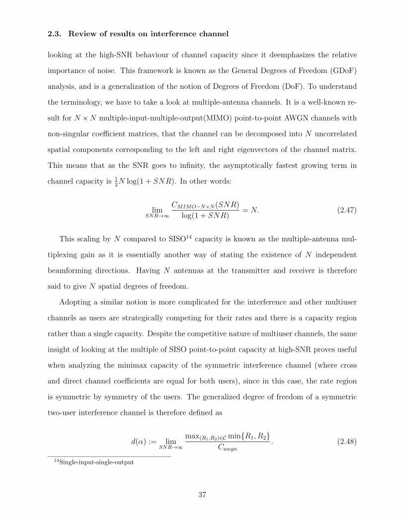
2.3. Review of results on interference channel
looking at the high-SNR behaviour of channel capacity since it deemphasizes the relative
importance of noise. This framework is known as the General Degrees of Freedom (GDoF)
analysis, and is a generalization of the notion of Degrees of Freedom (DoF). To understand
the terminology, we have to take a look at multiple-antenna channels. It is a well-known re-
sult for N ×N multiple-input-multiple-output(MIMO) point-to-point AWGN channels with
non-singular coefficient matrices, that the channel can be decomposed into N uncorrelated
spatial components corresponding to the left and right eigenvectors of the channel matrix.
This means that as the SNR goes to infinity, the asymptotically fastest growing term in
channel capacity is 12N log(1 + SNR). In other words:
limSNR→∞
CMIMO−N×N(SNR)
log(1 + SNR)= N. (2.47)
This scaling by N compared to SISO14 capacity is known as the multiple-antenna mul-
tiplexing gain as it is essentially another way of stating the existence of N independent
beamforming directions. Having N antennas at the transmitter and receiver is therefore
said to give N spatial degrees of freedom.
Adopting a similar notion is more complicated for the interference and other multiuser
channels as users are strategically competing for their rates and there is a capacity region
rather than a single capacity. Despite the competitive nature of multiuser channels, the same
insight of looking at the multiple of SISO point-to-point capacity at high-SNR proves useful
when analyzing the minimax capacity of the symmetric interference channel (where cross
and direct channel coefficients are equal for both users), since in this case, the rate region
is symmetric by symmetry of the users. The generalized degree of freedom of a symmetric
two-user interference channel is therefore defined as
d(α) := limSNR→∞
max(R1,R2)∈Cmin{R1, R2}Cawgn
. (2.48)
14Single-input-single-output
37

Chapter 2.
Here, Cawgn is the point to point capacity of the equivalent SISO channel. In this formulation,
DoF is characterized by an interference strength parameter α that defines the INR-SNR
scaling at high SNR’s, namely α := log INRlogSNR
, where α > 1 corresponds to strong and very
strong interference regimes and α < 1 represents weak interference. Generalized Degrees of
Freedom (GDoF) refers to this curve of d(α) showing the change in DoF of the channel as a
function of interference level. The work of Etkin, Tse and Wang [70] was the first to define
GDoF and obtain the now famous “W” shape of d(α) curve. Their work showed that for
values of α ∈ [0, 1/2] treating interference as noise is DoF-optimal. This was an observation
that was also made almost simultaneously by [71, 72, 73]. These results went against the
conventional view from the strong and very strong interference case that information-bearing
interference signals should not be discarded as noise. This was a crucial observation and one
that played a role in the application of interference alignment to interference channel which
we review in the next section.
2.4 Interference alignment
As we discussed in the previous section, the GDoF framework led to the observation that
for some operating regimes, not decoding interference might not be suboptimal. At the
same time a generalization of this analysis to K-user channels was done in [74]. For MIMO
and time-varying channels, where many independent dimensions are available, attention was
turned towards encoding schemes that try to concentrate interference terms and desired sig-
nal into disjoint subspaces. This is the essential idea of interference alignment and was first
used for capacity characterization in multiple-antenna X-channels (where each transmitter
has messages for each receiver) in [75]. In [11], Cadambe and Jafar show that fully con-
nected K-user interference channel with time-varying or frequency-selective coefficients can
effectively have 1/2 degrees of freedom per user for a total of K/2 as opposed to the 1/K
previously thought for a total of 1. This was a major result that has led a large number
38

2.5. Optimality of Treating Interference as Noise (TIN)
of follow-up publications investigating the applicability of interference alignment to other
channel models and also finding other methods of performing interference alignment. These
results include ergodic interference alignment [76], that can be applied to any channel at
finite SNR where coefficients are time varying and ergodic-in-time with a symmetric around
zero probability distribution, and real interference alignment [77] that uses the vector space
dimensions of real numbers over rationals and their number-theoretic properties to provide
dimensions over which to align signal and interference. The book [78] and survey article
[79] offer a more complete exposition of the main ideas behind and variations of interference
alignment. One common trait of these different variations is their perceived lack of practical
relevance. Some of this perception stems from the GDoF framework itself, where it has
been shown that the GDoF is an almost-everywhere discontinuous function of the channel
coefficients [80] and that the GDoF of interference channels collapses when channel state
information has finite precision [81], but also from the delay-rate trade-off of interference
alignment [82, 83], to the required feedback and synchronization overhead and finite-SNR
sub-optimality that results from ill-conditioned or incompletely specified channel matrices
[8].
2.5 Optimality of Treating Interference as Noise (TIN)
In an even more promising direction, recently the authors in [62] have shown that for a large
class of interference networks, treating interference as noise is GDoF optimal. This is done
by removing the power control variables from the formulation of the GDoF region. Using
the potential theory of network flow problems, they show that a polyhedral inner bound is
obtained by a certain relaxation of this problem and that it matches an outer bound based on
repeated application of the cyclic interference channel outer bounds of [84]. A more refined
analysis then shows that the total gap to sum capacity is in fact constant. This work has
been extended by [85, 86] both to gain insights into the relationship between combinatorial
39

Chapter 2.
problems and optimality of TIN and to extend it to other channel models. As mentioned,
this surprising result has already been used in [61] as the basis of a link scheduling algorithm
called ITLinQ which uses time sharing among subsets of links that satisfy the criteria of [62]
to service all links in a network.
The next two chapters concern the problems addressed in this thesis. Chapter 3 analyzes
a two-user cognitive channel and derives rate regions, decoder designs and rate optimization
strategies of the cognitive user. In Chapter 4, we study a large network link scheduling
problem and provide and analyze a scheduling method that has provable performance char-
acteristics with respect to the globally optimum schedule.
40

Chapter 3
Two-user cognitive GIC without
non-causal message information
In this chapter, we set up the model of Gaussian Interference Channel (GIC) with one cogni-
tive user that is the subject of our analysis. We then make the key observation that since the
legacy user cannot be realistically assumed to cooperate with the secondary user, a number
of techniques including time-sharing will not be available and therefore, the achievable rate
regions will be in general non-convex. This leads to a complicated rate optimization prob-
lems for the secondary (cognitive) user. Several rate-equivalent coding schemes are proposed
for this setup. The secondary rate-optimization problem is analyzed and its behaviour under
various regimes on parameter values classified. Part of the work in this chapter has been
previously presented in the paper [87].
The model that we have proposed here has elements of both underlay and interweave
setups. The secondary user both opportunistically senses whitespace in primary user’s band
and at the same time underlays part of its signal into the portion of the spectrum already
under use by this user. The secondary user must guarantee that the quality of service of the
primary does not fall below a certain threshold. The secondary receiver has the option to
apply joint decoding or treat interference as noise without relying on any cooperation from
41

Chapter 3. Two-user cognitive GIC
Figure 3.1: Band-limited Gaussian interference channel, BL(W1,W2) denotes the class ofsignals limited to the (W1,W2) band and Sz(f) is the spectral density of noise
the primary user. The problem that we solve on this model is determining the bandwidth
usage and power division strategy of the secondary user so that its rate is maximized subject
to the constraint on the rate of primary user.
3.1 The model and problem
In this section, the channel model and the problem we are trying to solved are described.
3.1.1 The channel model
The network topology in our model is the same as a Gaussian interference channel (shown
in Fig. 3.1, see also [65] and references therein). The total bandwidth is W and the static
and non-frequency selective channel coefficient from transmitter i to receiver j is denoted
by√aij. We assume the usual normalization convention discussed in Chapter 2, so we have
a11 = a22 = 1 without loss of generality. The noise is white, which means it has a flat spectral
42

3.1. The model and problem
density which is assumed equal to 1 by the same normalization convention. Transmitter i
is limited to a total power of Pi. User 1 is the primary (non-cognitive) user which has the
license to use the entire band. User 1 is unaware of the presence of user 2 which is the
cognitive or secondary user. Moreover, there is no cooperation among the users. Based on
its rate demand, user 1 only occupies a portion W0 of the whole bandwidth W .
3.1.2 The problem statement
With the channel model as above, user 2 is seeking to multiplex its data on the band W . It
occupies the whitespace W2 = W−W0 and to increase its transmission rate, it also underlays
part of its power over a portion Wc of the band W0 which is in use by user 1. This underlaying
is constrained by the quality of service condition R1 > Rth where Ri is the transmission rate
of user i and Rth is a fixed threshold on R1. The average transmission power of user 2 over
the bands Wc and W2 is Q and P2 −Q, respectively. Now the problem that user 2 is trying
to solve is that of maximizing its achievable rate without violating user 1’s rate constraint.
The optimization problem is formulated as
supWc,Q:Wc≤W0,Q≤P2
sup(R1,R2)∈R,R1>Rth
R2, (3.1)
where sup denotes the supremum (least upper bound) operation. R denotes the achievable
rate region for the two users where user 1 is using a legacy single-user encoder/decoder. In
other words, we are seeking a characterization of R and the maximum transmission rate
that user 2 can achieve when user 1 is achieving at least a rate Rth using simple single-layer
encoder/decoder architecture.
3.1.3 Example of a practical application
This problem is intended to model the scenario where a primary user with legacy equipment,
such as a VHF over-the-air TV broadcaster with licenses to a large number of analog VHF
43

Chapter 3.
channels, wants to coexist with an agile user that tries to use the bandwidth whitespace
for its own data transmission. Since the broadcaster may be in the process of phasing out
analog TV and some TV channels do not have constantly running programming, at any given
instance only a fraction of the assigned bandwidth is carrying data. To maximally assist
the secondary user in utilizing bandwidth the primary can announce its minimum requisite
quality of service which is modeled here by a rate constraint. To incentivize the primary user
to take part in sharing its bandwidth, the goal is to not impose any extra capital expenditure
requirements on it. Therefore, it is not required to upgrade its analog and near end-of-life
infrastructure to add the capability to dynamically announce which parts of the spectrum
are in use, for example by simultaneous out-of-band signaling. The burden of whitespace
detection, therefore falls on the cognitive user which is better-equipped to do it. The problem
facing the secondary user, after detecting the unused band, will be to divide its transmission
power over the empty and occupied parts of band in a way that maximizes its own rate
without violating QoS specification of the primary user. The primary user is not required
to change its equipment and transmission scheme, and is therefore has a higher incentive to
accept new uses for its band.
3.2 The achievable rate region R
Let both users utilize Gaussian codebooks. User 2 does not split its transmission rate
by separate coding over the private and common parts of the spectrum, i.e., the signals
transmitted over W2 and Wc belong to a codeword in a codebook of rate R2. At the receiver
side, user 2 has the option to apply simultaneous decoding or treat interference as Gaussian
noise, while user 1 only treats interference as Gaussian noise. Let us define
r1 := (W0 −Wc)C
(a1,2P1
W0
)+WcC
(Wca1,2P1
W0(Wc +Q)
), (3.2)
44

3.2. The achievable rate region R
s1 := W0C
(a1,2P1
W0
), (3.3)
r2 := (W −W0)C
(P2 −QW −W0
)+WcC
(W0Q
Wc(W0 + a1,2P1)
), (3.4)
s2 := (W −W0)C
(P2 −QW −W0
)+WcC
(Q
Wc
)(3.5)
and
t := (W0 −Wc)C
(P1
W0
)+WcC
(WcP1
W0(Wc + a2,1Q)
), (3.6)
where C(x) := log(1 + x). Then the rate region R is given by
R := {(R1, R2) : 0 < R1 < t}⋂({(R1, R2) : 0 < R1 < s1, 0 < R2 < s2, R1 +R2 < s1 + r2}⋃
{(R1, R2) : 0 < R2 < r2}). (3.7)
Fig. 3.2 shows the outline of R which is non-convex and resembles a chimney.
As an alternative coding scheme, user 2 can employ separate Gaussian codebooks over
the private and common parts of the spectrum, i.e., user 2 splits its rate R2 among two
independent codebooks transmitted over W2 and Wc separately. As before, user 2 has the
option to apply simultaneous decoding or treat interference as noise over the band Wc.
Denoting the achievable rate region under this alternative coding scheme by RRS, where
RS stands for rate-splitting, the following claim shows that RRS is the same as R given in
Equation 3.7.
Claim 3.1. Rate splitting gives the same region as joint coding, or RRS = R.
Proof can be found in Appendix A.
45

Chapter 3.
Figure 3.2: The chimney rate region R described in 3.7.
3.3 Remarks on encoder and decoder structure
In this section we describe two alternate achievable schemes that do not enlarge the rate
region calculated in the previous section, but are of independent interest as they provide
different encoder and decoder structures that achieve different trade-offs between simplicity
of the decoding rule and memory requirements of their implementation.
3.3.1 Non-unique joint typicality decoding
In the previous schemes discussed, user 2 has to adaptively choose between treating interfer-
ence as noise and simultaneous decoding. The authors of [69] and [88] have independently
proposed an alternative decoder structure which is applicable to our scenario as well. To de-
scribe this decoder, we have to describe joint typicality and its use in information-theoretic
46

3.3. Remarks on encoder and decoder structure
decoders. A deterministic n-sequence is called typical for probability distribution PX of
random variable X if the probability of it being observed in n independent draws of X is
between 2−(nH(X)−ε) and 2−(nH(X)+ε), for a small positive ε, where H(X) is the entropy of
X. Intuitively, this means that the empirical frequency distribution of letters in the se-
quence is very close to PX , so the the sequence is typical of what is seen in draws from
X. This definition straightforwardly extends to joint typicality for two or more sequences
with respect to a joint probability distribution, say PX,Y , and is called joint typicality. This
means that the empirical joint frequency distribution of the letters from these sequences is
close to that joint distribution. Almost all achievability results in information theory rely
on joint typicality decoding which means that the decoder tests all codewords for joint typ-
icality with the observed channel output with respect to the input-output joint probability
distribution. It declares success if and only if there is exactly one codeword jointly typical
with the output and declares the index of that codeword as the message sent. When jointly
decoding two codewords from a single channel output, the joint typicality of three sequences
(two codewords and one channel output) has to be considered and a decoding error is raised
even if the failure of unique joint typicality occurs for a message that is not intended for
our receiver. The decoder proposed by [69] and [88], relaxes this by implementing the rule
of joint typicality decoding with non-unique decoding for undesired message codewords1. It
turns out that using this so-called indirect decoder in our setup will achieve the same rate
region as derived before.
Claim 3.2. Replacing the decoder of Section 3.2 with a non-unique joint typicality decoder
will result in the same achievable region
Proof can be found in Appendix A.
So, as we saw, replacing the rather complex decoder structure of the previous section
achieves the same rates with considerably more elegance and operational simplicity, though
1This means that an error is not declared even if more than one codeword is jointly typical with thechannel output if they all agree on the desired message index.
47

Chapter 3.
at the expense of higher space (memory) complexity at the decoder. It is operationally
simpler because it achieves the same rate region with a unified one-step joint-typicality
decoder. This is in contrast with the decoder structure of the previous section that involves
implementing two joint-typicality decoders and selecting the output of the one giving the best
rate. This simplicity comes at a price though, since in a simple lookup table implementation,
this single joint-typicality joint decoder requires one lookup table of size 2R1+R2 , rather than
two successive lookup tables of size 2R1 and 2R2 respectively2.
3.3.2 Multi-layer encoding and successive cancellation
It is well-known that the corner points of the capacity region of a Multiple-access channel
can be achieved without resorting to simultaneous decoding. This is done by successive
interference cancellation (first used for decoding superposition codes in the paper by Cover
that introduced the broadcast channel [18]), where the message of one user is first decoded
and its effect subtracted from the channel output before decoding the message of the other
user. Normally, all other points on the boundary of the capacity region will be achieved
by time-sharing between these corner points. Unfortunately our setup does not allow for
time-sharing. Thus, it may seem that simultaneous decoding is inevitable in our scheme for
achieving points other than the corner points. This is not true however, since as it turns
out, with appropriate rate-splitting at the transmitter of user 2, successive cancellation of
interference can achieve all the boundary points. Our construction follows that of [89], the
details of which follow.
In the rate region achievable at receiver 2 in the previously discussed schemes, for the
points on the line R1 + R2 = s1 + r2 that are not corner points, it is implicitly assumed in
most practical designs that time-sharing between corner points can be used to achieve these
points using a simple interference cancellation scheme instead of the more computationally
demanding joint decoding at receiver 2. We recall that the specific setup of our problem
2This distinction might not be practically relevant since in both cases exponentially large lookup tablesare required.
48

3.3. Remarks on encoder and decoder structure
that precludes the cooperation by the primary, explicitly rules out this kind of time-sharing
cooperation and that this is indeed the reason that our rate region is non-convex. But,
while lack of cooperation leads to non-convexity of the achievable rate region it does not
mean joint decoding is the only way to achieve the non-corner points on the boundary of
the achievable region. Rimoldi et al. in [89] show that any point on the so-called dominant
face of the capacity region of a multiple-access channel (which in the case of the two-user
channel is exactly the set of rate pairs which attain the maximum sum-rate) can be achieved
by a computationally simple successive interference cancellation scheme. If we define the
function F (p, n) as
F (P, n) := log
(1 +
P
n
), (3.8)
which gives the twice the capacity of a discrete-time AWGN3 channel with power constraint
P and noise variance n, the function F satisfies
F (P1, n+ P2) + F (P2, n) = F (P1 + P2, n). (3.9)
A consequence of this identity is that , for a point-to-point Gaussian channel, any division
of rate by dividing the total power P1 + P2 between two superimposed codebooks with
powers P1, P2, when combined with a successive decoding scheme does not incur any rate
penalty or advantage. Likewise, in our own problem, if we focus on the two-user MAC
seen by user 2 over the band Wc, which has power constraints Wc
W0P1 and Q and gains
√a1,2 and 1 for users 1 and 2 respectively, then for any rate pair (R1, R2) on the sum-
rate boundary R1 + R2 = WcF(a1,2
Wc
W0P1 +Q,Wc
), user 2 can divide its power into Q1
and Q2 = Q − Q1 where Q1 is the unique non-negative number smaller than Q such that
R1 = WcF(a1,2
Wc
W0P1,Wc +Q1
)and generate a codebook C2,1 with rate R2,1 = WcF (Q2,Wc)
with power Q2 and another codebook C2,2 with rate R2,2 = WcF(Q2,WC + a1,2
Wc
W0P1 +Q1
)3Additive white Gaussian noise
49

Chapter 3.
and power Q2. We have that
F (Q2,Wc) + F
(a1,2
Wc
W0
P1,Wc +Q1
)+F
(Q2 ,Wc + a1,2
Wc
W0
P1 +Q1
)= F
(Q1 + a1,2
Wc
W0
P1 +Q2,Wc
)= F (a1,2
Wc
W0
P1 +Q,Wc).
(3.10)
Since the term on the right side of (3.10) is the sum-rate of the channel divided by Wc, we
can achieve this arbitrary rate pair by a two-layer encoding on the transmit side. On the
receive side, we recover the messages in a three-step process. We first decode C2,2, treating
the power contributed by C1 and C2,1 as noise. After that the message from C1 can be decoded
treating the power contributed by C2,1 as noise. Finally, we decode C2,1 and reconstruct user
2’s message (So the decoding order is C2,2 → C1 → C2,1).
The coding approach referred to in the previous section leads to another result and that
is a converse that multilayer random coding will not enlarge the rate region achievable by
our scheme.
We begin with a lemma that generalizes Equation 3.9.
Lemma 3.1. For the AWGN capacity function F defined by Equation 3.8, we have
n∑i=1
F (Pi, n+i−1∑j=1
Pi) = F (n∑i=1
Pi, n). (3.11)
Proof is by induction and can be found in Appendix A.
Claim 3.3. Multilayer random coding at user 2’s transmitter cannot enlarge the rate region
calculated in Section 3.2.
Proof can be found in Appendix A.
50
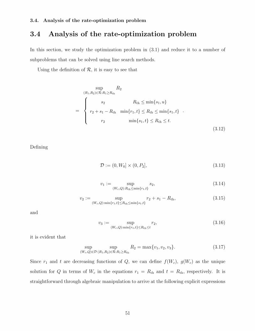
3.4. Analysis of the rate-optimization problem
3.4 Analysis of the rate-optimization problem
In this section, we study the optimization problem in (3.1) and reduce it to a number of
subproblems that can be solved using line search methods.
Using the definition of R, it is easy to see that
sup(R1,R2)∈R:R1≥Rth
R2
=
s2 Rth ≤ min{s1, u}
r2 + s1 −Rth min{r1, t} ≤ Rth ≤ min{s1, t}
r2 min{s1, t} ≤ Rth ≤ t.
.
(3.12)
Defining
D := (0,W0]× (0, P2], (3.13)
v1 := sup(Wc,Q):Rth≤min{r1,t}
s2, (3.14)
v2 := sup(Wc,Q):min{r1,t}≤Rth≤min{s1,t}
r2 + s1 −Rth, (3.15)
and
v3 := sup(Wc,Q):min{r1,t}≤Rth≤t
r2, (3.16)
it is evident that
sup(Wc,Q)∈D
sup(R1,R2)∈R:R1≥Rth
R2 = max{v1, v2, v3}. (3.17)
Since r1 and t are decreasing functions of Q, we can define f(Wc), g(Wc) as the unique
solution for Q in terms of Wc in the equations r1 = Rth and t = Rth, respectively. It is
straightforward through algebraic manipulation to arrive at the following explicit expressions
51

Chapter 3.
for f and g:
f(Wc) =
∞ Wc ≤W0
(1− Rth
s1
)+Wc
(2s1W0 −1
2s1W0 2
Rth−s1Wc −1
− 1
)+
Wc > W0
(1− Rth
s1
)+,
(3.18)
and
g(Wc) =
∞ Wc ≤W0
(1− Rth
R∗
)+Wca2,1
(2R∗W0 −1
2R∗W0 2
Rth−R∗Wc −1
− 1
)+
Wc > W0
(1− Rth
R∗
)+,
(3.19)
where x+ := max{x, 0} and R∗ := W0C(P1
W0
)is the maximum achievable rate for user 1 in
the absence of user 2. Noting that s1 is a constant, the conditions on Rth are seen to be
equivalent to
Rth ≤ min{r1, γ} ⇐⇒ Q ≤ min{f(Wc), g(Wc)}, (3.20)
min{r1, t} ≤ Rth ≤ min{s1, t} ⇐⇒
min{f(Wc), g(Wc)} ≤ Q ≤ g(Wc)1Rth≤s1 ,(3.21)
and
min{s1, t} ≤ Rth ≤ t ⇐⇒ g(Wc)1Rth≤s1 ≤ Q ≤ g(Wc), (3.22)
where 1{·} denotes the indicator function of a set.
Since r2, s2 and r2 + s1 − Rth are increasing functions of Wc, the optimizers in (3.14),
(3.15) and (3.16) are achieved on the boundary, i.e.
v1 = sup(Wc,Q)∈∂rmD1
s2,
D1 := {(Wc, Q) ∈ D : Q ≤ min{f(Wc), g(Wc)}} ,(3.23)
v2 := sup(Wc,Q)∈∂rmD2
r2 + s1 −Rth,
D2 := {(Wc, Q) ∈ D : min{f(Wc), g(Wc)} ≤ Q ≤
g(Wc)1Rth≤s1} ,
(3.24)
52

3.5. Relative magnitude of f and g
and
v3 = sup(Wc,Q)∈∂rmD3
r2,
D3 := {(Wc, Q) ∈ D : g(Wc)1Rth≤s1 ≤ Q ≤ g(Wc)} ,(3.25)
where for any region C in the x-y plane with boundary ∂C, ∂rmC denotes the “rightmost”
boundary of C defined by
∂rmC := {(x, y) ∈ ∂C : (x, y′) /∈ ∂C, ∀ y′ > y} . (3.26)
Next, we discuss some properties of the functions f and g that will help us in solving the
subproblems (3.23), (3.24) and (3.25).
3.5 Relative magnitude of f and g
The boundaries of D1 and D2 depend on the relative magnitudes of f and g. If f and g
intersect, the boundaries ∂rmD1 and ∂rmD2 may not be smooth curves. In the cases of weak
and strong interference, one of f and g dominates the other.
Claim 3.4. For the case of weak interference a1,2, a2,1 < 1, g(Wc) > f(Wc) for all Wc ∈
[0,W0]. For the case of strong interference a1,2, a2,1 > 1, g(Wc) < f(Wc) for all Wc ∈ [0,W0].
Proof can be found in Appendix A.
When interference is mixed, i.e., a1,2 > 1, a2,1 < 1 or a1,2 < 1, a2,1 > 1, f and g can
potentially intersect. It is easy to see that the equation f(Wc) = g(Wc) can be simplified as
(1− a2,1)2R∗+s1W0 2(2Rth−R∗−s1)Tc
+2R∗W0 (a2,12
β1W0 − 1)2(Rth−R∗)Tc
+2s1W0 (a2,1 − 2
R∗W0 )2(Rth−s1)Tc + 2
R∗W0 − a2,12
β1W0 = 0,
(3.27)
53

Chapter 3.
where Tc := 1Wc
. Descartes rule of signs [90] is useful for getting bounds on the number of
roots of a polynomial equation by counting sign changes in its sequence of coefficients. The
following lemma generalize Descartes rule of signs from polynomials to functions that are a
linear combination of exponential terms:
Lemma 3.2. The number of solutions of the equation a1eb1x + a2e
b2x + · · · + anebnx = 0 in
the real variable x where b1 < b2 < · · · < bn is at most the number of sign changes in the
sequence of coefficients (a1, a2, . . . , an) and has the same even-odd parity. In particular, any
such equation cannot have more than n− 1 solutions.
Proof runs along the same line as the proof of Descartes rule of signs and can be found
in Appendix A.
Using this Lemma, (3.27) can at most have three solutions in the real variable Tc. Note
that Tc = 0 is always a solution, however, this corresponds to Wc =∞ which is not accept-
able. As such, if the number of sign changes in the (properly sorted) sequence of coefficients
in equation (3.27) is two, there is exactly one finite value of Wc such that f(Wc) = g(Wc).
However, if the number of sign changes is three, the number of finite values Wc satisfying
f(Wc) = g(Wc) is either zero or two.
3.5.1 Characterizing the boundaries of D1, D2 and D3
We saw that the properties of the rate expressions characterizing our rate region are such
that the extreme value is taken on the boundaries where different rate expressions dominate.
These boundaries are given in terms of the functions f and g as defined above. In this
section, we characterize these boundaries.
Note that s1 is not dependent on the design parameters Wc and Q. If Rth > s1, then
Rth > min{r1, t} due to the fact that r1 ≤ s1. Hence, D1 is empty by (3.20) and (3.23). Also,
D2 is empty by (3.24). As such, one only needs to compute v3. If Rth ≤ s1, one needs to
find all v1, v2 and v3. In what follows, we discuss the cases Rth > s1 and Rth ≤ s1 separately
under various interference regimes:
54

3.5. Relative magnitude of f and g
Weak Interference (a12, a21 < 1)
• Rth > s1: In this case, only the rightmost boundary of D3 is of interest. This boundary
is comprised of the curve Q = g(Wc) : Wc ∈ [0,W0] and the vertical line segment
{W0} × [0, g(W0)].
• Rth ≤ s1: In this case, the rightmost boundaries of all D1, D2 and D3 are of interest.
Since g > f , ∂rmD1 consists of the curve Q = f(Wc) : Wc ∈ [0,W0] and the vertical
line segment {W0} × [0, f(W0)], ∂rmD2 consists of the curve Q = g(Wc),Wc ∈ [0,W0]
and the vertical line segment {W0} × [f(W0), g(W0)] and ∂rmD3 consists of the curve
Q = g(Wc) : Wc ∈ [0,W0]. Therefore, ∂rmD3 ⊂ ∂rmD2. Since Rth ≤ s1, we have
r2 + s1 − Rth ≤ r2 for given Q and Wc. Hence, v3 ≤ v2 and computing v3 is not
necessary.
Strong Interference (a12, a21 > 1)
• Rth > s1: In this case, only the rightmost boundary of D3 is of interest. This boundary
is comprised of the curve Q = g(Wc) : Wc ∈ [0,W0] and the vertical line segment
{W0} × [0, g(W0)].
• Rth ≤ s1: In this case, the rightmost boundaries of all D1, D2 and D3 are of interest.
Since f > g, ∂rmD1 consists of the curve Q = g(Wc) : Wc ∈ [0,W0] and the vertical line
segment {W0} × [0, g(W0)] and ∂rmD2 and ∂rmD3 coincide and are represented by the
curve Q = g(Wc),Wc ∈ [0,W0]. Since Rth ≤ s1, we have r2 + s1−Rth ≤ r2 for given Q
and Wc. Hence, v3 ≤ v2 and computing v3 is not necessary. Note that ∂rmD2 ⊂ ∂rmD1,
however, r2 + s1 −Rth = s2 + r1 −Rth may be smaller or larger than s2. As such, one
is required to compute both v1 and v2.
55
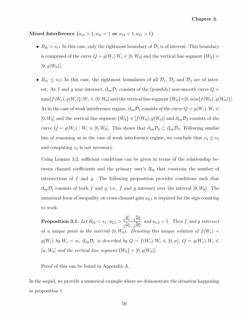
Chapter 3.
Mixed Interference (a12 > 1, a21 < 1 or a12 < 1, a21 > 1)
• Rth > s1: In this case, only the rightmost boundary of D3 is of interest. This boundary
is comprised of the curve Q = g(Wc)Wc ∈ [0,W0] and the vertical line segment {W0}×
[0, g(W0)].
• Rth ≤ s1: In this case, the rightmost boundaries of all D1, D2 and D3 are of inter-
est. As f and g may intersect, ∂rmD1 consists of the (possibly) non-smooth curve Q =
min{f(Wc), g(Wc)},Wc ∈ (0,W0] and the vertical line segment {W0}×[0,min{f(W0), g(W0)}].
As in the case of weak interference regime, ∂rmD2 consists of the curve Q = g(Wc),Wc ∈
[0,W0] and the vertical line segment {W0} × [f(W0), g(W0)] and ∂rmD3 consists of the
curve Q = g(Wc) : Wc ∈ [0,W0]. This shows that ∂rmD3 ⊂ ∂rmD2. Following similar
line of reasoning as in the case of weak interference regime, we conclude that v3 ≤ v2
and computing v3 is not necessary.
Using Lemma 3.2, sufficient conditions can be given in terms of the relationship be-
tween channel coefficients and the primary user’s Rth that constrain the number of
intersections of f and g. The following proposition provides conditions such that
∂rmD1 consists of both f and g, i.e., f and g intersect over the interval [0,W0]. The
unnatural form of inequality on cross-channel gain a2,1 is required for the sign-counting
to work.
Proposition 3.1. Let Rth < s1, a2,1 >2R∗W0 −2
RthW0
2s1W0 −2
RthW0
and a1,2 < 1. Then f and g intersect
at a unique point in the interval (0,W0). Denoting this unique solution of f(Wc) =
g(Wc) by Wc = w, ∂rmD1 is described by Q = f(Wc),Wc ∈ [0, w], Q = g(Wc),Wc ∈
[w,W0] and the vertical line segment {W0} × [0, g(W0)].
Proof of this can be found in Appendix A.
In the sequel, we provide a numerical example where we demonstrate the situation happening
in proposition 1.
56

3.6. Possible extreme cases of the problem
3.6 Possible extreme cases of the problem
We have analyzed and broken down the rate optimization problem into its constituent sub-
problems. In this section we discuss under which conditions the optimum Wc obtained will
be equal to W0 and 0 respectively. as these two cases correspond to when it’s optimal to
share the entire primary user’s band and sharing exactly nothing
3.6.1 Wc = 0
In our formulation of the problem, if Rth > s1, the optimal power-bandwidth relationship is
given by g, likewise if Rth < s1, it is given by min{f, g}. Now, the functions f and g have
both vertical asymptotes at a positive non-zero Wc at and to the left of which they both
go to infinity. Since practically, Q is also limited by user 2’s available power P2, this means
that for values of Wc smaller than the asymptote, including zero, the optimal Q equals P2.
On the other hand, for a fixed power budget clipped at P2, rate is monotone increasing in
Wc, hence Wc = 0 could not be optimal.
3.6.2 Wc = W0
This case, that corresponds to the total band of primary user being shared can actually
happen. One numerical example that this case is indeed possible is W = 3,W0 = 2, P1 =
P2 = 100, a12 = 0.1, a2,1 = 2.2, Rth = s15
where the optimal Wc equals W0 and gives R2 ≈
7.336.
3.7 Numerical Examples
To give a better insight into the performance of the proposed scheme, this section provides
a number of numerical examples.
First, we consider a scenario where W = 8 Hz, W0 = 6 Hz, P1 = 7 dB, P2 = 9 dB,
57

Chapter 3.
0 1 2 3 4 5 60
1
2
3
4
5
6
7
8
The region D1
Wc (Hz)
Q(W
atts)
Figure 3.3: The region D1.
a1,2 = 67
and a2,1 = 52. In this case, R∗ = 5.6141 bits/sec/Hz and s1 = 4.6742 bits/sec/Hz.
Assume Rth < β1, say, Rth = 3.5057 bits/sec/Hz.4 As discussed in the previous section,
we only need to compute v1 and v2. The regions D1 and D2 are shown in Fig. 3.3 and
Fig. (3.4), respectively. Note that the region D2 is the union of the shaded region and
the tail-like curve extending from Wc = 2.62 Hz to Wc = 6 Hz. Note that ∂rmD1 has a
breaking point at (Wc, Q) = (2.62, 4.601). It turns out that Wc = 2.62 Hz is the solution
for f(Wc) = g(Wc). In fact, the part of ∂rmD1 extending from Wc = 2 Hz to Wc = 2.62 Hz
is the curve Q = f(Wc) and the part extending from Wc = 2.62 Hz to Wc = 6 Hz is the
curve Q = g(Wc). This observation is consistent with the result of proposition 1. In fact,
2R∗W0 −2
RthW0
2β1W0 −2
RthW0
= 1.5238. Since a2,1 > 1.5238, Rth < s1 and a1,2 < 1, the point Wc = 2.62 Hz5
in fact the unique solution w to f(Wc) = g(Wc) as verified by proposition 1. Fig. 3.5, Fig.
3.6 and Fig. 3.7 demonstrate the values of objective functions ∂rmD1 and ∂rmD2. It is seen
that the optimum tuple (Wc, Q) is given by (Wc, Q) = (5.36, 6.05) which occurs on the part
of ∂rmD1 represented by Q = min{f(Wc), g(Wc)}.4We have Rth
R∗ = 0.6244.5While the frequencies used here are too small to be practically relevant, we note that this is an artifact
of the chosen input parameters W and W0 being small. As is customary in information theory literature,small parameter values are selected so that performance parameters can be demonstrated with relativelysmall numbers. Similar analysis carries over for multi-megahertz bandwidths as well.
58

3.7. Numerical Examples
1.5 2 2.5 3 3.5 4 4.5 5 5.5 61
2
3
4
5
6
7
8
The region D2
Wc (Hz)
Q(W
atts)
Figure 3.4: The region D2.
0 1 2 3 4 5 60
0.5
1
1.5
2
2.5
3
3.5
Wc (Hz)
β2(bits/sec)
Figure 3.5: Plot of s2 in terms of Wc on the part of ∂rmD1 represented by Q =min{f(Wc), g(Wc)}.
3.7.1 Maximum can be attained in different parts of the boundary
In this section, we provide a few concrete numerical examples to show how the point that
achieves the maximum rate can be moved to different parts of the boundary by changes in
value of the problem parameters. We assume that W = 3 Hz, W0 = 2 Hz, P1 = P2 = 20 dB,
a12 = 0.1 and a21 = 2.2. Now we can see that if we set Rth = 1.5 bits/s, then the maximum
will be taken on the rightmost boundary of the region of definition of v2 and in particular the
59

Chapter 3.
0 0.2 0.4 0.6 0.8 1 1.2 1.4 1.6 1.82.3
2.4
2.5
2.6
2.7
2.8
2.9
3
3.1
3.2
Q (Watts)
β2(bits/sec)
Figure 3.6: Plot of s2 in terms of Q on the part of ∂rmD1 that is a vertical line segment
1.5 2 2.5 3 3.5 4 4.5 5 5.5 62.2
2.4
2.6
2.8
3
3.2
3.4
3.6
3.8
Wc (Hz)
α2+
β1−
Rth
(bits/sec)
Figure 3.7: Plot of r2 + s1 −Rth in terms of Wc on ∂rmD2 represented by Q = g(Wc).
Wc = 2 Hz and Q = 63.33 Watts. For the same problem, if we set Rth = 2.02 bits/s, then the
maximum will be taken on the topmost boundary of the region of v2 for Wc = 1.91 Hz and
Q = 57.76 Watts. More interestingly for Rth = 1.63 bits/s the maximums at the topmost
and rightmost boundaries coincide at Wc = 2 and Q ≈ 59.03 Watts.
60

3.8. Shape of the rate curve
3.7.2 Sensitivity of achievable rates to changes in parameter val-
ues
To see how the behaviour of the maximum achievable rate changes with changes to parameter
values, we demonstrate here how changes in a12 and Rth affect the achievable rates, holding
all other parameters constant. For W = 1Hz, W0 = 0.7Hz, P1 = P2 = 100, a12 = 0.6 and
a21 = 26, Fig. 3.8 shows the effect of changing Rth on the maximum achievable R2. Similarly
for W = 1Hz, W0 = 0.7Hz, P1 = P2 = 100 and a21 = 2, Fig 3.9 shows the effect of changing
a12 on the maximum achievable R2 for the case that Rth is chosen to be 0.33s1.
0.1 0.2 0.3 0.4 0.5 0.6 0.7 0.8 0.9 1 1.12.6
2.7
2.8
2.9
3
3.1
3.2
3.3
3.4
3.5
Rth
Rmax
2
Figure 3.8: Plot of maximum achievable R2 as a function of changing R∗.
3.8 Shape of the rate curve
To complete our numerical examples, in this section, we also provide examples of the overall
shape of the rate region. In figure 3.10 you can see the maximum value of R2 attainable by
this scheme for W = 5, W0 = 2, a1,2 = 0.5, a2,1 = 5 and P1 = P2 = 10dB as a function of
R1 = Rth. The rate region is also calculated for W = 5, W0 = 2, a1,2 = 0.2, a2,1 = 0.2 and
6As discussed previously, small round numbers are used for input parameters, as is customary in informa-tion theory literature, to be able to demonstrate the example without having to deal with many significantdigits.
61

Chapter 3.
0 0.5 1 1.5 2 2.5 32.8
2.85
2.9
2.95
3
3.05
3.1
3.15
3.2
3.25
3.3
a12
Rmax
2
Figure 3.9: Plot of maximum achievable R2 as a function of changing a12.
P1 = 17dB P2 = 13dB as is shown in figure 3.11. As can be seen, this region is not in general
convex.
3.9 Conclusion
Thus far, we proposed and analyzed the interference channel with one cognitive user. We
proposed a series of achievability schemes for this channel that all achieve the same rate
region, but do so by emphasizing different components of the trade-off between conceptual
and computational simplicity of coding and decoding schemes. We then analyzed the rate
optimization problem that the cognitive secondary user faces and noted its non-convexity.
The structure of this problem was exploited to reduce its solution to a number of subproblems
of smaller dimension. Rigorous results were obtained on the structure and interrelationship
of these subproblems in different interference strength regimes. Numerical examples were
provided to supplement these results and shed light on the behaviour of our problem and
give an idea of its performance for some ranges of parameters.
62

3.9. Conclusion
0.5 1 1.5 2 2.5 3 3.5 4 4.5 5 5.50
1
2
3
4
5
6
7
8
P1=10dB, P
2=10dB, g
12=0.5, g
21=5, W=5, W
0=2
R2
R1*
Achievable rate region (R2 as a function of R
1* )
Figure 3.10: Achievable rate region for W = 5, W0 = 2, a12 = 0.5, a21 = 5 and P1 = P2 =10dB
63

Chapter 3.
1 2 3 4 5 6 70
1
2
3
4
5
6
7
8
9
R1*
R2
Achievable rate region (R2 as a function of R
1* )
P1=17dB, P
2=13dB, g
12=0.2, g
21=0.2, W=5, W
0=2
Figure 3.11: Achievable rate region for W = 5, W0 = 2, a1,2 = 0.2, a2,1 = 0.2 and P1 = 17dBP2 = 13dB
64

Chapter 4
Approximate link scheduling in large
networks
This chapter concerns the second part of the thesis that deals with the problem of SINR-
feasible link scheduling in large wireless networks. Contrasting the approach taken in the
previous chapter, we turn our attention from the two-user networks to the issue of interfer-
ence management in the presence of large number of interfering users. The scale of these
networks makes complex encoding and decoding schemes impractical and leaves only the
simplest transmitter and receiver design strategies like treating interference from structured
messages of other users as added noise. These simplified approaches are not without theoret-
ical basis. As noted previously, the importance of interference management and interference
control has been put on theoretically firm ground by the advent of degrees-of-freedom (DOF)
analysis and interference alignment (IA) that put the burden of interference management on
the transmitter and treat whatever remains at the receiver as noise. But these approaches,
based mostly on channel-state dependent transmitter-side constellation designs, have offered
limited prospects for large-scale practical applications due to excessive complexity of channel-
code design and encoding operations[12, 13, 82]. Recently, a series of results have emerged
that show near-optimality of treating-interference-as-noise (TIN) without any transmitter
65

Chapter 4. Approximate link scheduling in large networks
side signal shaping for large classes of interference networks [62, 85]. This has paved the
way towards providing a more direct mapping from theory to practice in interference man-
agement, and suggests an approach that is particularly suited to scenarios encountered in
emerging large Machine-to-Machine (M2M) and Device-to-Device (D2D) networks. These
developments stress the importance of treating Signal to Interference as Noise Ratio (SINR)
itself as a key metric to optimize for attaining the best achievable rates in large networks, in-
stead of seeing it just as an approximation to the true capacity metric whose only advantage
is simplicity of analysis. Inspired by these results, new heuristic SINR-aware wireless schedul-
ing algorithms have appeared in the literature including the previously reviewed FlashLinQ
[60] and ITLinQ [61] that aim at producing higher-throughput link schedules that target
SINR levels and are not computationally expensive. As discussed previously, this combina-
tion of theoretical and practical developments means that investigating approaches to link
scheduling that are simple, scalable and have theoretically provable performance guarantees
is an important research direction. This chapter, after defining a network model and stating
the scheduling problem formally, describes an approximate scheduling algorithm that has
provable performance guarantees and show that it performs well in practice, specially as the
size of the network grows.
The outline of the rest of the chapter is as follows. Section 4.1 describes the model.
Section 4.2 gives a formal definition of the minimum length scheduling problem. In sec-
tion 4.3 the problem of finding the minimum-length schedule is formulated as a mixed in-
teger program. Using this framework, mathematical programs are given that are amenable
to solution using optimization tools such as CPLEX[91] and Gurobi[92]. Mixed integer
programming gives exact solutions but the time and memory requirements grow very fast
with the instance size, therefore an alternate formulation is given that can be repeatedly
solved to obtain successively refined lower bounds1 and feasible solutions and which provides
an interval containing the exact minimum length and accommodates larger instance sizes.
1A lower bound is inferred when the MIP solver declares that the instance has no feasible integer solutionwith the given schedule length.
66

4.1. Model and assumptions
Next, an approximation algorithm for the solution of the link scheduling problem based on
graph-theoretical ideas is proposed. This algorithm takes advantage of the geometric struc-
ture imposed by the metric space of the link endpoints to decompose the links into subsets
having specific properties and uses a specialized scheduling algorithm as a subroutine to
separately schedule subsets of the resulting decomposition. The proposed algorithm finally
composes these sub-schedules into an approximate schedule for the general-form input in-
stance. Section 4.4.1 defines the criteria based on which this decomposition process takes
place. This section also gives notation and definitions for other properties that are used
to further describe the scheduling algorithm and specify its approximation ratio. This al-
gorithm and its building blocks are introduced in Section 4.4.2. This includes a flow-chart
of the top-level method as well as the special-case approximate scheduling algorithm that
is used as a subroutine. The description of the steps these algorithms take is accompanied
with a series of lemmas establishing their correctness and approximation ratio. Proofs of
these lemmas are outlined but the details are relegated to Appendix B. Finally, we report on
numerical experiments and conclude this chapter in Section 4.5. Part of the work described
in this chapter has been previously presented in the paper [93].
4.1 Model and assumptions
This section describes the underlying model of the wireless network. Our model considers a
set of {1, ..., L} links. Each link l ∈ L is characterized by the tuple (o(l), d(l), p(l), G(l)).
The points o(l), d(l) are the origin and destination points of link l. These points are
only constrained to be in a doubling metric space M2. The use of doubling metric space
assumption is technical as we make use of triangle inequality and doubling constraint in
proving some lemmas. To make this technical assumption more intuitive, the reader can
2A doubling metric space is a metric space for which there are constants C and m such that every ball
B(p, r) of radius r can contain at most C(
r′
r
)mdisjoint balls of radius r′. The number m is called the
doubling dimension of the metric space.
67
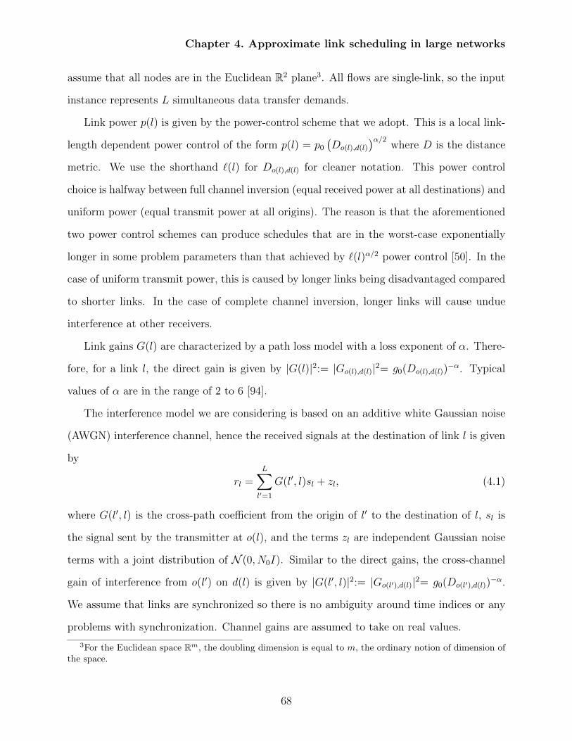
Chapter 4. Approximate link scheduling in large networks
assume that all nodes are in the Euclidean R2 plane3. All flows are single-link, so the input
instance represents L simultaneous data transfer demands.
Link power p(l) is given by the power-control scheme that we adopt. This is a local link-
length dependent power control of the form p(l) = p0(Do(l),d(l)
)α/2where D is the distance
metric. We use the shorthand `(l) for Do(l),d(l) for cleaner notation. This power control
choice is halfway between full channel inversion (equal received power at all destinations) and
uniform power (equal transmit power at all origins). The reason is that the aforementioned
two power control schemes can produce schedules that are in the worst-case exponentially
longer in some problem parameters than that achieved by `(l)α/2 power control [50]. In the
case of uniform transmit power, this is caused by longer links being disadvantaged compared
to shorter links. In the case of complete channel inversion, longer links will cause undue
interference at other receivers.
Link gains G(l) are characterized by a path loss model with a loss exponent of α. There-
fore, for a link l, the direct gain is given by |G(l)|2:= |Go(l),d(l)|2= g0(Do(l),d(l))−α. Typical
values of α are in the range of 2 to 6 [94].
The interference model we are considering is based on an additive white Gaussian noise
(AWGN) interference channel, hence the received signals at the destination of link l is given
by
rl =L∑l′=1
G(l′, l)sl + zl, (4.1)
where G(l′, l) is the cross-path coefficient from the origin of l′ to the destination of l, sl is
the signal sent by the transmitter at o(l), and the terms zl are independent Gaussian noise
terms with a joint distribution of N (0, N0I). Similar to the direct gains, the cross-channel
gain of interference from o(l′) on d(l) is given by |G(l′, l)|2:= |Go(l′),d(l)|2= g0(Do(l′),d(l))−α.
We assume that links are synchronized so there is no ambiguity around time indices or any
problems with synchronization. Channel gains are assumed to take on real values.
3For the Euclidean space Rm, the doubling dimension is equal to m, the ordinary notion of dimension ofthe space.
68

4.2. Formal definition of scheduling problem
We make the major simplifying assumption that the links are single-rate, so we impose
the uniform SNR threshold of β. We require that
γl =p(l)G(l)
N0 +∑l′ 6=l
l′ active with l
P (l′)Gl′l
≥ β,
for link l to do a successful transfer. In practice, β as a parameter is a function of physical
layer technology, RF chain sensitivity and the desired bit-error-rate.
With the elements of the network model described, the next section defines the problem
that we are trying to solve.
4.2 Formal definition of scheduling problem
The model of the network was defined in the previous section. We are now ready to give a
formal definition of the scheduling problem. The problem input instance is a set of network
links {1, ..., L}. Also, two sets of parameters are used to characterize the exact conditions
under which the network operates. The first set of parameters is a function of the ambient
space that our link endpoints operate in (which is itself assumed to be a metric space M
with doubling dimension m and distance measure D). They are the path loss exponent α,
noise spectral density N0 and the normalized unit distance gain g0. The second set consists
of parameters characterizing the radio hardware at the link endpoints and consists of the
normalized transmit power p0 and receiver SNR threshold β. Each link in the input instance
is characterized by the tuple (o(l), d(l), p(l), G(l)) where o(l), d(l) are the free parameters
characterizing the link’s origin and destination. They fully characterize the other two com-
ponents of the tuple as p(l) := p0Dα/2o(l),d(l) and |G(l)|2:= g0D
−αo(l),d(l). As noted before, the
shorthand notation `(l) := DO(l),d(l) is used for the length of link l. Using this shorthand,
link transmit power and gain can be written as p(l) = p0`(l)α/2 and |G(l)|2= g0`(l)
−α, respec-
tively. As shown by equation 4.1, the effect of interference is modeled by an additive channel
69

Chapter 4.
with cross-gains of |G(l′, l)|2= g0D−αo(l′),d(l) from link l′ on link l. As described previously, all
gains are real-valued and the noise is white, Gaussian-distributed and additive.
The output corresponding to an input instance, the optimum schedule, consists of a
partition of {1, ..., L} into subsets {s1, ..., sS}, such that each l is in exactly one st, or
t, t′ ∈ {1, ..., S}, t′ 6= t⇒ St ∩ St′ = ∅ (4.2)
S⋃t=1
st = {1, ..., L}, (4.3)
(4.4)
and for each st, all links l ∈ st satisfy
∀st,∀l ∈ st γl :=p(l)G(l)
N0 +∑
l′ 6=l∈st P (l′)Gl′l≥ β. (4.5)
Also, and crucial to optimality, the cardinality S of the partitioning {s1, ..., sS} is minimum
among all such partitions satisfying the above criteria.
It is clear that having such optimum {s1, ..., sS}, we can associate each st to a different
time instant such that all transfer requests are satisfied and this is the shortest length of
timeslots in which this can happen. This justifies the name minimum-length schedule.
The sets si satisfying the above criteria are called, in analogy to vertex-independent sets
of a graph, scheduling-independent sets or ISets for short. With this terminology, optimum
scheduling is the problem of partitioning the set {1, ..., L} into the minimum number of ISets.
Formally, the parameters, input and output of the optimum link scheduling problem are:
Parameters: path loss exponent α, metric M , dimension m and associated distance
measure D, Noise spectral density N0, normalized gain g0 and power p0 and SNR threshold
β.
Input: a set of links {1, · · · , L} with each link l associated to the tuple (o(l), d(l), p(l), G(l))
of which o(l), d(l) determine the other two components based on the parameters. Similarly
70

4.2. Formal definition of scheduling problem
the cross gains G(l, l′) are defined by the path loss formula as described before.
Output: a number S and sets s1, s2, . . . , sS such that:
1. st’s are disjoint and cover all of {1, ..., L}.
2. st’s are scheduling ISets as defined previously.
3. Their cardinality, S is minimum among all partitions satisfying the previous two con-
ditions.
It is obvious that this problem has a well-defined, computable solution. In particular,
the cardinality S of the partitioning is at least 1 and at most L and there is only finitely
many partitions of {1, ..., L} to examine and find the smallest consisting only of ISets.
If the problem output specification above is relaxed to finding, instead of the exact
minimum partition, a partition whose length is approximately close to minimum, we will
have the problem of approximate link scheduling. For a positive non-decreasing function h
of instance size and parameters, an algorithm for the approximate link scheduling problem
is said to O(h)-approximate link scheduling if the ratio of the length of its output schedule
to the minimum-length output schedule asymptotically grows like O(h).
4.2.1 Example of a practical application scenario
A scenario where solving this problem is useful is for a large-scale network of autonomous
radio devices arranged in peer-to-peer setup. An example of this is a large scale device-to-
device network of autonomous vehicles or drones. The network will operate over consecutive
rounds where a static set of demands declared at the start of the round are serviced in a
finite number of transmission timeslots before the start of the next round. In order to max-
imize utilization of the network, we want to conclude each round in as small a number of
transmission slots as possible. A scheduling algorithm decides on the number of timeslots
and the links transmitting in each timeslot of the round. Therefore, an exact or approximate
71

Chapter 4.
solution to finding the minimum number of timeslots required to schedule a set of transmis-
sion requests allows achieving the highest possible link utilization and minimizes the time
between successive rounds. Having a scalable algorithm is important if the size of network
is large or if limited computational resources are available at each node.
4.2.2 Complexity of exact scheduling
As discussed previously, the scheduling problem can in principle be solved by exhaustively
examining all partitions of the set {1, ..., L} and producing the one that has the smallest
cardinality (length) and consists only of β-SINR feasible ISets. This brute force approach
does not exploit any structure present in the problem instance and takes exponential time
in L. Therefore, solving the SINR-based minimum-length with more clever algorithms and
characterizing its worst-case performance is an important problem. Since many simpler
versions of link scheduling, for instance graph-based independent set scheduling discussed
previously are equivalent to NP-complete problems (such as producing vertex colourings of
general graphs), it might seem reasonable to assume that the problem defined above is NP-
complete as well. This is not a rigorous argument as there might be a smart way of exploiting
the structure inherent in the problem to drastically cut down on the time required to solve
it. In contrast, formally showing that this problem is NP-hard, involves finding a way of
reducing general instances of an already known NP-complete problem to it. This section
reviews the literature on the complexity of link scheduling problem.
Apart from results on graph vertex colouring, Turong et al. in [95] were the first to
look at the complexity of wireless link scheduling. They consider an interference model
where the two-hop neighbourhood of any two transmitting nodes should be disjoint and
show that obtaining the optimal schedule in this setting is NP-complete. Borbash et al. in
[96] consider the problem of SINR-based scheduling without geometric constraint on channel
gains and show a reduction to it from a generalized graph-matching problem which they
hypothesize to be NP-complete. Later, Behzad et al. in [97] gave a linear programming
72

4.3. Mixed integer programming formulation
formulation of the minimum-length scheduling with a SINR metric that is of exponential
size in problem parameters. They also proved, by a reduction from instances of graph edge-
colouring problem to their formulation, that SINR-based scheduling with general channel
coefficients is NP-Complete. Both of these reductions lead to arbitrary matrix of channel
gains without any geometric structure. Of more interest to our case, Goussevskaia et al. in
[51] showed that even instances of minimum-length SINR-based scheduling where channel
gains are constrained to be related to link lengths by a path loss formula are still expressive
enough to represent general instances of NP-complete problems. In particular, they show
through a reduction from general instances of set-partitioning problem to geometric instances
of SINR-based scheduling, that even in this restricted setting, scheduling is NP-complete.
This result definitively establishes that the problem we are trying to solve is NP-complete.
This makes it imperative to look at approximate solutions for larger instances. The next
section shows that scheduling can be formulated as a mixed integer program in a format
that is suitable for mathematical programming software and that these software tools can
be used to find exact solutions for intermediate-sized instances.
4.3 Exact solution of scheduling using a mixed integer
program
Having formally defined the problem of finding exact minimum-length SINR-feasible sched-
ule and looked at its complexity, this section formulates this problem as an instance of
Mixed Integer Programming (MIP). This allows us to enlist the well-developed MIP-solving
capabilities of general-purpose optimization software for its solution. The standard MIP for-
mulation also serves as a concise alternative formal definition of the problem. Before that,
we briefly discuss the subject of mixed integer programming.
A mixed integer program is an optimization problem (mathematical program) in which
the objective function and constraints are linear functions of the variables and with the
73

Chapter 4.
added constraint that some variables only take on integer values. The addition of integrality
constraints distinguishes these problems from linear programs (LP) and gives them extra
expressive power. This expressiveness comes with the disadvantage that standard simplex
and interior point methods are not adequate for solving MIP instances. In the worst case,
solving MIP’s requires solving an exponentially large number of LP instances corresponding
to fixed choices for the values of discrete variables. Still, there is a group of well-developed
techniques for pruning this search tree of discrete choices which, together with heuristics for
ordering these choices, makes many mixed integer programs of interest effectively solvable.
For general MIP problems, these techniques include the branch and bound [98] and branch
and cut [99] methods. Both of these methods require many calls to LP solvers on intermediate
instances obtained by relaxations of the original program and use the results to further
prune the set of remaining tree nodes they have to examine. This reliance on search tree
pruning in general MIP solving strategies has consequences both in formulating combinatorial
optimization problems as MIP instances and in the choice of successive relaxations that
solvers internally make. One example is that in formulating a problem as a mixed integer
program, there is often a trade-off between the work done per node of the search tree and the
number of nodes that need to be examined on average. A formulation with more constraints,
which leads to an increase in the size of intermediate LP instances, can prune the search tree
nodes more effectively on average and therefore be more efficient overall. A formulation with
less constraints, on the other hand, solves smaller intermediate LP instances but might need
to look at a larger fraction of the search tree nodes. In any case, the framework of general
mixed integer programs is so expressive that it can represent every NP-complete problem,
so there is good reason to believe that this exponential search tree complexity might be
inherent.
The problem we are trying to solve is a general set partitioning problem with extra
constraints, where these constraints needs to only hold between elements that are inside the
same subset of the partition (namely, the SINR feasibility constraint of link has to hold only
74

4.3. Mixed integer programming formulation
relative to links in the same partition as itself). One way to formulate this problem is to use
binary indicator variables indexed by both link and ISet indices to signify when a link belongs
to a certain ISet. The SINR feasibility constraint on a link when receiving interference from
all links in some ISet, then, will only need to hold if the indicator variable of the link in that
ISet is 1. It seems hard at first to express this logical constraint activation without using
multiplication and when confining ourselves to linear expressions in the indicator variables.
The big-M trick [100] is a method in mathematical programming that can be used, among
other things, to formulate these logical constraints that are not strictly linear, as linear
constraints of a specialized form. As mentioned, the SINR constraint is of this logical
type as its incorporation is predicated on the link belonging to a certain ISet. Using the
big-M trick, a constraint activation condition such as our SINR feasibility criterion will be
incorporated by subtracting from the right hand side of the unconditional constraint written
as a ≥ inequality, a large number M4 times the indicator variable of interest. With this extra
term, whenever the indicator variable is 1, the inequality is vacuously satisfied and does not
further constrain other variables involved.
With this primer, two formulations are presented next. The first formulation uses a
smaller number of constraints and is symmetric under renaming ISet indices. It has many
feasible solutions corresponding to what is qualitatively the same scheduling solution and as a
result can require a larger branch and bound tree. The second formulation, on the other hand
tries to order the ISet indices by their cardinality and breaking ties lexicographically. This is
done in order to make the correspondence between MIP and original problem solutions one-
to-one and the search tree smaller. This comes at the cost of extra constraints to enforce
this ISet ordering, which increase the size of relaxed instances that need to be solved at
intermediate nodes of the branch and bound tree.
4Hence the name big-M.
75

Chapter 4.
4.3.1 First approach
Similar to what we did for links in the general formulation, we equate the ISets Ss with
their index s, so that both links and ISets are identified with integers. This helps make the
mathematical programs that follow cleaner. With this convention, the lowercase l is used to
index the set of links and lowercase s the set of ISets. Using indicator variables xls to denote
link l belonging to set s, the problem of minimizing the schedule length can be formulated
as the mathematical program below (with the use of shorthand notation [N ] for the set
{1, ...N}):
minS,{xls}
S
s.t. xls ∈ {0, 1} S ∈ N,∀l ∈ [L],∀s ∈ [S]S∑s=1
xls = 1 ∀l ∈ {1, .., L}
xlsG(l)p(l) ≥ xlsβN0 +∑l′ 6=ll′∈s
xl′sp(l′)G(l′, l)−M(1− xls) ∀l ∈ {1, .., L},∀s ∈ {1, ..., S}.
(4.6)
As can be seen, The first constraint signifies that xls is the binary indicator of whether or
not link l is put into partition s. The second constraint states that the schedule should be
valid, that is every link should be scheduled exactly once. The last constraint uses the big-M
trick to enforce the SINR constraint only when a link belongs to an ISet.
This formulation is a straightforward translation of the problem. Unfortunately, since the
range of indices for variables xls depends on another program variable S, this formulation
does not strictly conform to the definition of MIP. This can be overcome as will be discussed
shortly, but a variation of this formulation, as a mixed integer feasibility problem5 can be
used as a decision procedure to determine whether a certain number of ISets suffices for a
given set of links. As such, repeatedly solving of this variation can give successively tighter
5In an MIP feasibility problem, the goal is to only determine whether the feasible region of a set of MIPconstraints is nonempty.
76

4.3. Mixed integer programming formulation
feasible solutions and infeasible schedule lengths which act as upper and lower bounds for
the exact solution. When these bounds meet, we know that we have that exact solution.
Conversion to this feasibility problem works by replacing the range of s in xls with the
constant s0 for which we want to check if there is a solution with that many ISets. This will
lead to the following program:
min{xls}
2
s.t. xls ∈ {0, 1} ∀l ∈ [L], ∀s ≤ s0s0∑s=1
xls = 1 ∀l ∈ {1, .., L}
xlsG(l)p(l) ≥ xlsβN0 +∑l′ 6=ll′∈s
xl′sp(l′)G(l′, l)−M(1− xls) ∀l ∈ {1, .., L},∀s ∈ {1, ..., s0},
(4.7)
which has the constant 2 as the dummy objective to show that it is only the feasibility of
constraints that are important. For any given s0, the above problem is feasible if and only
if s0 is equal to or greater than the minimum schedule length for that instance. This is a
proper MIP feasibility problem. The difference between Programs 4.6 and 4.7 can be seen
by way of an example:
Assuming that we have a set of L = 100 links represented as L = {1, ..., 100} and we like
to determine an interval containing the optimum schedule length. It is very unlikely that
all links are simultaneously feasible, and it is also unlikely that 100 individual timeslots are
required. Therefore a reasonable first guess might put the optimum value in the range of 15
77

Chapter 4.
to 35 ISets. If the program
min{xls}
2
s.t. xls ∈ {0, 1} ∀` ∈ L,∀s ∈ {1, ..., 35}35∑s=1
xls = 1 ∀l ∈ L
xlsG(l)p(l) ≥ xlsβN0 +∑l′ 6=ll′∈s
xl′sp(l′)G(l′, l)−M(1− xls) ∀j ∈ N,
(4.8)
is feasible and replacing 35 by 15 makes it infeasible, our initial guess of [15, 35] is validated
and we can tighten the range to, say [20, 30]. Otherwise, depending on the solution of the
two programs, the range should be enlarged from one end until it contains the exact solution.
By successively tightening the upper and lower ends of the range, the exact optimum s can
be found. An advantage of this formulation is that the gradual refinement of the interval
means that we have an upper and lower bound to the exact answer even computation is
stopped before the exact solution is pinpointed.
Program 4.6 can be converted to a proper MIP by noting that S is at most L (the
ISets are singleton sets in the worst case). The range of indices for xls can now be changed
accordingly. To accommodate the new possibility that some of the L ISet indices may not
be used, a new set of indicator variables ys can be added that indicates whether the s’th
78

4.3. Mixed integer programming formulation
ISet is empty or not. With these changes, the program below results:
minS,{xls},ys
S
s.t. xls ∈ {0, 1} ∀l, s ∈ {1, ..., L}L∑s=1
xls = 1 ∀l, s ∈ {1, ..., L}
ys ∈ {0, 1} ∀s ∈ {1, ..., L}
ys ≥ xls ∀l, s ∈ {1, ..., L}
ys ≤L∑l=1
xls ∀s ∈ {1, ..., L}
L∑s=1
ys = S
xlsG(l)p(l) ≥ xlsβN0 +∑l′ 6=ll′∈s
xl′sp(l′)G(l′, l)−M(1− xls) ∀j ∈ N.
(4.9)
The added constraints on the ys’s enforce that ys represents the non-emptiness of ISet s and
that their sum is equal to the variable S which is also the program objective.
As pointed to previously, this mixed integer program has many solutions corresponding
to any distinct solution of the original problem, all of which are equivalent up to a relabel-
ing of the ISet indices s. In practice, a general-purpose branch and bound solver without
information about this symmetry might need to look at a much larger number of search
tree nodes than absolutely required to conclude that it has exhausted all possibly better
solutions.
4.3.2 Adding ordering constraints to reduce symmetry
The formulation in the previous section was a straightforward translation of problem objec-
tive and constraints. It had the disadvantage that each qualitatively distinct solution of the
original problem was equivalent to large number of MIP solutions by relabeling of the in-
dices s. The formulation presented here tries to alleviate this blowup using extra constraints
79

Chapter 4.
that favour smaller indices s for the larger ISets and break ties by lexicographic ordering of
the elements of [L]. Using similar notation and indicator variables names, xls, ys as in the
previous section, this formulation adds two extra constraints as presented below:
minS,{xls},ys
S
s.t. xls ∈ {0, 1} ∀l, s ∈ {1, ..., L}L∑s=1
xls = 1 ∀l, s ∈ {1, ..., L}
ys ∈ {0, 1} ∀s ∈ {1, ..., L}
ys ≥ xls ∀l, s ∈ {1, ..., L}
ys ≤L∑l=1
xls ∀s ∈ {1, ..., L}
ys+1 ≤ ysL∑s=1
ys = S
xlsG(l)p(l) ≥ xlsβN0 +∑l′ 6=ll′∈s
xl′sp(l′)G(l′, l)−M(1− xls) ∀j ∈ N
L∑l=1
xls ≥L∑l=1
xl,s+1 ∀s ∈ {1, ..., L− 1}
L∑l=1
lxls ≥L∑l=1
lxl,s+1 −M ′(L∑l=1
xls −L∑l=1
xl,s+1) ∀s ∈ {1, ..., L− 1}.
(4.10)
The last constraint uses a big M’ value to enforce ordering by cardinality (the other parts of
the constraint enforce lexicographic ordering when cardinalities are equal). The second to last
constraint requires smaller s indices to be used for nonempty ISets first before using larger
s values. The SINR criterion with the big-M trick is the same as the previous formulation,
as are the constraints used to enforce xls and ys representing a proper partitioning of [L].
These mixed integer programs can be solved using standard mathematical programming
software such as CPLEX [91] and Gurobi [92] to obtain the exact solution. As it will be
discussed in Section 4.5, programs 4.9 and 4.10 become prohibitive for instances of larger
80

4.4. Proposed approximate algorithm
than about 50 and 30 links respectively. As such, in that section, we use the bounding
approach along with program 4.7 to compare the proposed algorithm with the interval bounds
containing the exact solution, for medium-sized instances of up to 250 links. With the MIP
formulations of the exact problem provided, the next section turns attention to the proposed
approximate scheduling algorithm, where its operation is described and correctness and
approximation ratio are established.
4.4 The proposed algorithm for approximating the op-
timum schedule
This section defines the scheduling algorithm of our schemes and provides an analytical
treatment of its performance. We first give a preliminary account of the top-level organization
of this algorithm together with required definitions in Section 4.4.1. Detailed discussion of the
algorithm and lemmas and theorems characterizing its performance are given in Section 4.4.2.
4.4.1 Notation and preliminaries
We defined the notation used for the links and described what an ISet is while formally
defining the minimum-length scheduling problem. This section is both a recap of those and
also defines new terms that are used in describing our approximate scheduling algorithm.
The set of intended transmit-receive pairs is denoted by set {1, 2, . . . , L} of links as before,
where each link l represents a transmitter located at o(l) and a receiver at d(l). The distance
metric between two points p1 and p2 is being denoted by D(p1, p2) := Dp1,p2 and we use the
shorthand Dl,l′ = Do(l),d(l′). As previously noted, `(l) := Do(l),d(l) denotes the length of link
l.
We use the notation [L] for the set {1, ..., L}, and more generally [N ] for a set {1, ..., N}
of numbers from 1 to N , in subscripts and in other places when it causes less clutter. Also, to
harmonize our notation with what is customary for representing instance sizes in discussion
81

Chapter 4.
of algorithmic complexity, we denote the size of [L], which is the number L as n. Using this
notation, we define ∆, the ratio of longest to shortest link as: ∆ :=maxl∈[L] `(l)
minl∈[L] `(l).
Length class: a length class or an almost equilength class is a set of links the lengths
of which do not vary by more than a factor of two. As we will see, it is sometimes easier to
divide a set of links into a number of length-classes and treat each class separately.
Normalized ISR and affectance: we first note that the Interference-to-Signal ratio
(ISR) between a two links is
I ′l′(l) =p(l′)/D(l′, l)α
p(l)/`(l)α.
This can be generalized to ISR of a set S on a link defined as
I ′S(l) =
∑(l′ 6=l)∈S p(l
′)/D(l′, l)α
p(l)/`(l)α.
Similarly for total ISR sent from a link to links on a set S, we have
I ′l(S) =∑
(l′ 6=l)∈S
p(l)/`(l)α
p(l′)/`(l′)α.
The definition of I ′S1(S2) is analogous. An advantage of this notion is additivity, that is
I ′S1∪S2(l) = I ′S1
(l) + I ′S2(l) for disjoint S1 and S2.
In order to normalize this metric with respect to β, we use the notion of affectance. This
variation of ISR, first introduced in [52] and refined in [54] and [55] is defined as
Il′(l) := min
(1, gl
p(l′)/D(l′, l)α
p(l)/`(l)α
)= min
(1, gl
p(l′)
p(l)·(
`(l)
D(l′, l)
)α),
where the factor gl := β/(1 − βN0`(l)α/p(l)) depends only on properties of the link l and
problem parameters. This can be analogously extended to affectance to and from sets as
Il(S) :=∑
l′∈S Il(l′), IS(l) :=
∑l′∈S Il′(l), and IS(T ) :=
∑l′∈S Il′(T ) for sets S and T . It is
82

4.4. Proposed approximate algorithm
easy to see that a set S being an ISet is equivalent to IS(l) < 1 for each l ∈ S.
As a first step in the scheduling algorithm, we pass from the geometric arrangement of
nodes in a metric space to an abstract graph. The vertices of this graph correspond to
network links and vertex connectivity is based on geometry of the network in a way that
helps us build the approximation to the optimum link schedule. In order to go from the
notion of an SINR-feasible ISet which defines a hypergraph on vertices representing links to
a binary edge-connectivity relation between link pairs, we use a pairwise relaxation of the
SINR feasibility of an ISet. What we mean by a relaxation is that if a subset of links forms
an ISet, then all of its pairs of links will be disconnected in this relaxed notion. The reverse
relationship, of a subset that is vertex-independent according to this binary relation being
SINR-feasible and therefore an ISet, does not necessarily hold. This has the advantage of
enabling us to use the conceptual simplicity of graph theory while still remaining close to
the SINR formulation. We will see that the conflict graph built on this notion provides lower
bounds on length of any SINR-feasible schedule. More importantly, the relaxed notion is still
strong enough that it can be used advantageously in the design of our scheduling method
and yet the conflict graphs built on it are structured enough to be efficiently colourable.
This is the notion of q-independence defined next.
q-independence: parameterized by a number q, q-independence is a pairwise relaxation
of the notion of SINR-feasibility. Formally, two links l′ and l are q-independent if they satisfy
D(l′, l) ·D(l, l′) ≥ q2 · `(l)`(l′). This is equivalent to Il(l′) · Il′(l) ≤ glgl′
q2α, independent of the
power scheme used. If two links are not q-independent, they are called q-dependent or q-
adjacent since they are adjacent in the graphic representation of this relation. Likewise, a
set of links is called q-independent if all pairs of its links are q-independent and its called
q-dependent otherwise.
The q-dependence graph is defined by having a vertex for each link and having an edge
between two vertices whenever they are q-dependent.
From the above definition, it is easy to see that if two links are q-dependent they cannot
83

Chapter 4.
be simultaneously active in a qαβ-SINR feasible ISet (that is an ISet that satisfies the more
stringent qαβ SINR criterion), but the reverse will not necessarily be true as interference
power is accumulative.
The q-dependence graph of [L] is represented by Gq([L]). Recall that this graph has
vertices corresponding to all links in [L] and an edge between two vertices whenever their
respective links are q-dependent.
The top level of the proceeds by first colouring Gq([L]). This is done by a greedy subrou-
tine which takes linear time in the number of edges and vertices of the graph. It produces a
vertex-colouring that, using a special property of Gq([L]), is shown to use at most a constant
factor more colours than the its chromatic number, which is by definition, the minimum
number of colours required for a vertex colouring of this graph.
Since q-independence is, as noted, a relaxation of the notion of SINR-feasibility of ISets,
this colouring can serve as a rough first step in putting links whose simultaneous transmission
directly leads to SINR conflicts into different ISets.
The next step considers each monochromatic set, which is by definition a q-independent
subset of [L], separately when allocating ISets to avoid obvious pairwise conflicts between
q-dependent links. In order to build an ISet partition for each such q-independent monochro-
matic subset, we will have to define a few more refined properties that allow bounding of
sum-interference from other links when putting a link into a tentative ISet. The next few
definitions explicitly define these properties between pairs or subsets of links. The roles these
conditions play and the way they are satisfied at various stages of the algorithm is clarified
in the next section. To motivate the definitions though, they are accompanied by a short
description of how they help in different stages of the scheduling.
τ-interfering links: two links l, l′ are said to be τ -interfering if max{Il(l′), Il′(l)} > τ ,
that is at least one is causing a normalized ISR of more than τ on the other. Later, when
we try to assign links to different ISets (timeslots) using a greedy binning approach, we use
properties of this definition with an appropriately defined value of τ to show that the chosen
84

4.4. Proposed approximate algorithm
number of bins is enough.
Lengthwise well-separated link set: a set of links is lengthwise well-separated if for
every link l, and all longer links l′, we either have that `(l′) < 2`(l) or `(l′) > 2.(4n)2α `(l).
Informally, what this says of a set is that the length relationship between any pair of links in
it is such that they are either almost equilength or else have widely differing lengths. Noting
that the length ratio in the second case is a growing function of instance size n, this notion
helps in making an argument based on pigeonhole principle that the total interference from
certain types of links on others is bounded.
p-greedily binnable link-set: parameterized by a natural number p, a subset A ⊆ [L]
is said to be p-greedily binnable if for every link in [L], there are at most p-links in the
set that are both 2.(4n)2α -times longer than it and 1
2n-interfering with it. This is where the
τ -interfering property mentioned earlier is used. When a group of subsets have this property,
their links can be aggregated in p+1 bins corresponding to different ISets in a greedy manner
while assuring that the total interference any link receives in its assigned ISet is bounded.
4.4.2 Description of the algorithm, its correctness and perfor-
mance
In this section, using the definitions just provided, we state our algorithm and characterize its
correctness and approximation ratio using a series of lemmas. During its operation, the top-
level algorithm invokes a greedy graph colouring algorithm and a special-case link scheduling
algorithm (which requires its input instance to satisfy certain conditions) as subroutines.
When discussing each of these algorithms, a compact description the steps of the algorithm
is given first, then the operation of the algorithm is discussed step-by-step together with
lemmas that show correctness and bounds on the approximation ratio. For each lemma, a
high-level overview of why it holds and the role it plays in showing the overall correctness
and performance of the algorithm is given, but longer derivations and proofs are relegated
to Appendix B. As stated previously, the power control scheme assigns power proportional
85

Chapter 4.
to `(l)α/2 due to the advantages this choice offers compared to both uniform power and
complete channel inversion. Nevertheless, in one particular stage of the algorithm, when
considering links within a length class (where, as we saw, lengths differ within a factor of at
most 2), we will state and use a lemma about uniform transmission powers and use the fact
that since the lengths do not differ by a factor more than 2, uniform and `(l)α/2-power are
in a certain sense, very similar.
As one last note, the ultimate goal of this algorithm is to partition a set of transmission
requests into a set of ISets feasible with SINR β so that members of different ISets can be
active over successive timeslots. At the same time, we are trying to make the cardinality of
this partition as close to the minimum cardinality as possible. In what follows, therefore,
we use the terms timeslots and ISets interchangeably. In principle, different ISets could
be assigned to different frequency bands, which would make the objective equivalent to
minimizing the number of frequency channels, but this is not relevant to the structure of the
problem.
Algorithm 1 is the top-level algorithm that we use for scheduling a set of links:
Algorithm 1 Scheduling arbitrary sets of links.
1. Construct the q-dependence graph for q = 3, G3([L]) on the set of links [L].
• We have the graph G3([L]) at this stage.
2. Colour G3([L]) using Hochbaum’s greedy colouring algorithm.
• After this step, we have [L] split into 3-independent subsets L1, L2, . . . , Lk wherek is at most cχ(G3([L]) by Theorem 4.1.
3. For i = 1, 2, . . . , k apply Algorithm 3 to the set Li.
• After this step, we get for each i, a partition of Li into a collection of ISetsΣi = {S1
i , S2i , . . . , S
kii }, where ki is the cardinality of the collection.
4. The output schedule is the set of all ISets in collections calculated for different Li’s:∪iΣi
The flowchart of this algorithm is shown in Figure 4.4.2. The algorithm starts by con-
86

4.4. Proposed approximate algorithm
Yes
Star
t Ev
ent
Form
the
adja
cenc
y m
atrix
on
q-d
epen
denc
e gr
aph
of th
e lin
ks,
Initi
aliz
e an
em
pty
stac
k fo
r ver
tex
orde
ring
In o
rder
, fro
m to
p to
bot
tom
of t
he
vert
ex s
tack
, ass
ign
to e
ach
vert
ex
the
smal
lest
col
our i
ndex
not
use
d by
its
pre
viou
sly
colo
ured
nei
ghbo
urs,
ca
ll th
e re
sulti
ng m
onoc
hrom
atic
cl
asse
s K
j
Each
Kj is
a le
ngth
cl
ass
and
q in
depe
nden
t so
it pr
ovab
ly is
fe
asib
le w
ith S
INR
~(
q/4)
α β w
hen
pow
er c
ontr
ol is
un
iform
Any
ver
tices
left
Rem
ove
min
imum
deg
ree
vert
ex
from
the
grap
h an
d pu
sh it
to th
e st
ack
It ca
n be
con
verte
d to
a S
ched
ule
of
cons
tant
leng
th a
nd
SIN
R β
2α/2
+1fe
asib
le
call
this
sch
edul
e S j
Switc
hing
from
un
iform
to s
quar
e ro
ot p
ower
con
trol
mak
es it
at w
orst
SI
NR
2 fe
asib
le
(ISR
½)
Switc
hing
from
un
iform
to s
quar
e ro
ot p
ower
con
trol
mak
es S
j at w
orst
SI
NR
2β
feas
ible
(N
orm
aliz
ed IS
R ½
)
Now
eac
h B i
is q
-in
depe
nden
t and
th
eref
ore
prov
ably
(lo
g(lo
g(∆)
)+1)
-gr
eedi
ly b
inna
ble
If q>
3
Firs
t Sor
t lin
ks in
des
cend
ing
orde
r and
put
them
in th
e fir
st ti
mes
lot w
here
the
sum
ISR
from
alre
ady-
put (
long
er)
links
is le
ss th
an th
e ne
w S
INR
, the
n in
eac
h tim
eslo
t bin
go
thro
ugh
links
in a
scen
ding
leng
th o
rder
and
sub
divi
de
into
new
tim
eslo
t bin
s su
ch th
at s
um IS
R fr
om a
lread
y-pu
t (s
horte
r) lin
ks is
sm
alle
r tha
n de
sire
d
A se
t is
p-gr
eedi
ly b
inna
ble
if at
mos
t p li
nks
exis
t th
at a
re b
oth
long
er th
an it
s lin
ks b
y a
fact
or 2
(4n)
2/α
and
are
mor
e th
an 1
/(2n)
-inte
rferin
g
(log(
log(∆)
)+1)
-bin
nabi
lity
mea
ns
that
1st ,2
nd …
slo
ts o
f Sj‘s
for
diffe
rent
j ca
n be
gre
edily
spr
ead
into
log(
log(∆)
)+2
slot
s by
pi
geon
hole
prin
cipl
e w
ith a
t mos
t
1/2n
ISR
on
each
link
from
link
s in
ot
her S
j‘s
Putti
ng a
ll st
eps
toge
ther
, eac
h B i
is
sche
dule
d in
to lo
g(lo
g(∆)
)+2
slot
s, e
ach
mon
ochr
omat
ic s
et o
f the
q-in
depe
nden
ce
grap
h ha
s cl
og(n
) Bi’s
and
the
grap
h is
co
lour
ed w
ith ‘cχ’
diff
eren
t col
ours
Putti
ng th
e sc
hedu
les
of d
iffer
ent B
i’s a
fter
one
anot
her t
hus
give
s us
our
sch
edul
e of
le
ngth
cχl
og(n
)log(
log(∆)
) jj
nj
ij
iK
QB
¥ =ú úù
ê êé ++
¥ ==
=1
)4
log
21.(
1U
Ua
{[
] }m
inm
in1
2,2
)(
ll
li
ii
ll
Q-
Î=
Figure 4.1: Flowchart for Algorithm 1.
87

Chapter 4.
structing the q-independence graph. As can be seen, q = 3 is chosen in step 1 above. This
choice is justified by the fact that it leads to subsets that satisfy the input conditions of
Algorithm 3 invocation in step 3 as will be discussed later. This step has worst case time
complexity O(n2) which is the maximum number of edges of the graph.
Step 2 uses a greedy algorithm to vertex-colour G3([L]). The greedy colouring algorithm
used is due to Hochbaum [101]. There, it is shown to have a complexity of O(|V |+|E|) on a
graph with vertex set V and edge set E, which corresponds to a worst-case time complexity of
O(n2) in our notation. This is Algorithm 2, called greedy Min-Degree-Last and the following
lemma characterizes its performance for q-independence graphs.
Algorithm 2 Greedy Min-Degree-Last vertex colouring
input : Graph G.Output : A vertex colouring of graph G, with colours indexed by integers 1 and above.
1. Obtain the total order Min-degree-last on graph G as follows:
(a) Initialize an empty stack for the vertices.
(b) Select v a vertex of minimum degree in G.
(c) Remove v and its incident edges from G, push v onto the stack.
(d) Go to step (b) and continue removing until all vertices are removed.
(e) After the above steps are finished, the top-to-bottom order of vertices on thestack is the desired total order, inductively defined such that each vertex is hasthe minimum degree in the graph induced by itself and vertices coming before itin the order.
2. Go through vertices in Min-degree-last ordering (so the last vertex remaining in theprevious step comes first here) and colour each vertex with the smallest colour notused by any of its adjacent predecessors.
Lemma 4.1. Algorithm 2 is a greedy colouring algorithm that colours any q-independence
graph Gq using cχ(Gq) colours for c a constant.
Proof: The proof is based on showing that the neighbourhood of each vertex in Gq
has a bounded maximum independent set size. To show this, the geometric structure of the
connectivity in Gq is used. The details are in Appendix B.
88

4.4. Proposed approximate algorithm
Step 3 of the Algorithm 1 relies on Algorithm 3. Invocation of this Algorithm is where
most of the scheduling work happens. We defined the notion of p-greedily-binnable subsets
previously and briefly discussed how this property is useful by allowing greedy aggregation of
links from different p-greedily-binnable subsets into a set of p+ 1 separate bins. Algorithm 3
requires the set of links at its input be q-independent and p-greedily binnable. Under these
conditions, the output of this algorithm will be a collection of ISets of cardinality O(p log n).
Algorithm 3 Scheduling q-independent and p-greedily binnable sets of links.
Input : A q-independent p-greedily binnable set Q, for some p > 0 and q ≥ 1.Output : A partition of Q into O(p log(n)) ISets.
1. Let Q = ∪iQi, where Qi = {l ∈ Q|`(l) ∈ [2i−1`min, 2i`min)}, for i = 1, 2, . . . , imax ≤
dlog(∆)e.
2. Assign Bi = ∪iQi+j·(1+d 2αlog 4ne), for 1 ≤ i < 1 + d 2
αlog 4n)e.
3. Schedule each Bi = ∪jKj, where Kj := Qk+j·(1+d 2αlog 4n)e, using the steps that follow:
(a) Using the SINR-strengthening lemma from Theorem 4.3 transform each Kj into
an e-SINR feasible partition of ISets: Σj = {Ssj}kjs=1 under uniform power with
e = 2α/2+1β.
• After this step we have a collection of subsets of Kj, each of which is an ISetfeasible with SINR 2α/2+1β under uniform power. Since, maximal pairwiselength ratio is 2, changing power control from uniform to `(l)α/2 means thateach ISet is at the worst 2β-SINR feasible.
(b) s← 1.
(c) Assign S ← ∪jSsj : if for some j, kj < s, then we take Ssj = ∅.(d) Sort S in the non-increasing order of link lengths: `1 ≥ `2 ≥ . . . `|S|.
(e) T rs ← ∅, r = 1, 2, . . . , p+ 1.
(f) For k = 1, 2, . . . , |S| do: find a T rs not containing links u with `u > 2.(4n)2α `k
which are 1/(2n)-interfering with k, and assign T rs ← T rs ∪ {k}.(g) s ← s + 1: if s ≤ max kj, then go to step 3.(c), otherwise the schedule for Bi is{T rs |T rs 6= ∅}.
4. Output the union of the schedules of all Bi.
The flowchart of Algorithm 3 is shown in Figure 4.4.2. Step 1 of this algorithm decom-
poses the input set of links into a series length classes, sets where maximum link length ratio
89

Chapter 4.
Divi
de th
e lin
ks in
to
max
imal
leng
th cl
ass s
ets
(l max
/l min≤2
), th
e Q
j’s
Gath
er u
p Q j
’s w
here
link
le
ngth
s diff
er b
y at
leas
t 2(
4n)2/
α toge
ther
into
wel
l-se
para
ted
sets
Bi
Expa
nd e
ach
of th
e Q j
’s fro
m a
s ~(q
/4)α β
-un
iform
-feas
ible
into
a 2
α/2+
1 β-u
nifo
rm-
feas
ible
par
titio
n se
quen
ce {S
j} (a
nd n
ote
that
sinc
e le
ngth
ratio
is ≤
2 th
ey
are
2β-fe
asib
le in
(ℓ)α/
2 -pow
er)
For e
ach
B i, e
ach
Qj in
it, e
ach
times
lot i
n th
e 2β
-feas
ible
pa
rtiti
on {S
j} as
socia
ted
to th
is Q j
, Allo
cate
log(
log(∆)
)+3
empt
y IS
et b
ins:
Go th
roug
h lin
ks, l
ong
to sh
ort,
and
put e
ach
link
in th
e fir
st
slot f
or w
hich
it re
ceiv
es ≤
1/(2
n) IS
R fro
m li
nks i
n di
ffere
nt Q
j‘s
Outp
ut: S
ets Q
jOu
tput
: c.lo
g(n)
sets
Bi
Each
Gat
herin
g Se
ts Q
j of
wid
ely
diffe
ring
leng
ths
Outp
ut: 2
β-fe
asib
le
part
ition
sequ
ence
s {S
j} co
rres
pond
ing
to
each
Qj
Outp
ut: l
og(lo
g(∆)
)+3
new
Iset
s per
ea
ch Is
et in
dex o
f all
part
ition
s {S j}
m
ade
from
eac
h Q j
that
bel
ongs
to th
e sa
me
B i
Glue
all
the
sche
dule
s cor
resp
ondi
ng to
eac
h di
ffere
nt ti
mes
lots
inde
x ins
ide
each
Bi
Outp
ut: a
sche
dule
of c
.(log
(log(∆)
)+3)
tim
eslo
ts fo
r eac
h B i
Conc
aten
ate
sche
dule
s cor
resp
ondi
ng to
diff
eren
t B’
s
Outp
ut: a
sche
dule
of
c.(lo
g(lo
g(∆)
)+3)
.log(
n) ti
mes
lots
for t
he
set Q
Inpu
t: a
set Q
pr
oduc
ed b
y al
gorit
hm 2
Figure 4.2: Flowchart for Algorithm 3.
90

4.4. Proposed approximate algorithm
is at most 2, namely the Qi’s. Step 2 then takes the union of Qi’s whose indices differ by
an integer multiple of 1 +⌈log(
(4n)2α
)⌉into the maximal well-separated sets Bi. Recall
that a well-separated set is a set of links where for every pair the length ratio is either less
than 2 or more than 2.(4n)2α , so step 2 forms the maximal well-separated subsets of Q in
the most straightforward way. It is also simple to see that exactly 1 +⌈log(
(4n)2α
)⌉sets
Bi are formed at the end of this step containing all the links in Q. When discussing the
operations of step 3, it is useful to denote the j’th subset in the union defining Bi, that is
the set Qi+j.(1+dlog((4n)
2α )e)
by Kj, with its dependence on i being implicit.
Step 3.(a) refines each set Kj := Qi+j.
(1+⌈log((4n)
2α
)⌉) into a collection of its subsets that
are SINR feasible ISets for SINR level 2α/2+1β. The correctness of this step relies on two
lemmas.
The first lemma and the only place that we rely on uniform power in this derivation is
a result that shows the one-way implication from SINR-feasibility to q-Independence, which
results from the latter being a relaxation of the former, has a restricted converse. More
precisely, if a set of links is a length class, has maximal pairwise link length ratio at most
2, and all pairs of links are q-independent, It will be SINR-feasible for a certain SINR level
kβ (k > 1) with uniform power control. The sets Kj are by definition q-independent and
length class subsets and satisfy this condition. The following lemma states this restricted
equivalence between SINR-feasibility and q-independence.
Lemma 4.2. Any almost equilength class of links in a doubling metric space that is q-
independent is also SINR feasible under uniform power assignment.
Proof: To bound the total interference to a given receiver, this proof accounts for the
interference from transmitters of other links located inside different concentric rings around
this receiver separately. An argument based on the geometric definition of q-independence,
together with all pairs of links being almost equilength, puts an upper bound on the number
of transmitters in each ring using the doubling property of the metric. This leads to a bound
on total interference from transmitters in k’th concentric ring for each integer k. Summing
91

Chapter 4.
over all k gives a desired bound on total interference that implies the link SINR criterion is
met. The full details are in Appendix B
The next ingredient in showing the correctness of step 3.(a) is noticing that different SINR
levels are interchangeable in the sense that an ISet that is feasible for a certain SINR level
can be refined into a collection of a constant number of its subsets, each of which are feasible
for a given higher target SINR level. This is shown by the following SINR-strengthening
result:
Lemma 4.3. [SINR strengthening] Any collection of S-SINR feasible ISets can be refined
into a collection S ′-SINR feasible subsets (S ′ > S), increasing the cardinality of the collection
by at most⌈(
2S′
S
)⌉2.
Proof: The proof is rather simple and proceeds by judiciously dividing each ISet of the
original collection into a number of ISets in a two-step greedy process, such that the new
ISets are feasible for the higher SINR level. The complete proof can be found in Appendix B.
Application of the previous lemma in step 3.(a) decomposes each Kj into a constant
number of its subsets Ssj ’s, each of which is an ISet with SINR level 2α/2+1β under uniform
power. Since the pairwise link length ratios in these ISets is upper-bounded by 2, changing
power control from uniform to `(l)α/2 makes the ISets Ssj feasible for SINR 2β in the worst
case.
Steps 3.(b) to 3.(g) depend on the assumption that the input set of links is p-greedily
binnable. The following lemma states that if q ≥ 3, this property holds for inputs given to
Algorithm 3 by the top-level Algorithm 1. This is where the arbitrary-seeming value of 3
comes from in step 1 of that algorithm.
Lemma 4.4. Any q-independent set of links for q ≥ 3 is O(log log ∆)-greedily binnable.
Proof: At a high level, this proof uses the geometric definition of q-independence and
the triangle inequality in the metric space of nodes to establish a lower bound on the length
ratio of two-links that are both at least 2.(4n)2α times longer than a given link l, mutually
92

4.4. Proposed approximate algorithm
q-independent with each other, and more than 12n
-interfering with l. This bound implies a
doubly exponential growth rate on the lengths of successively longer links of this type which
is then used to upper bound their total number. Full details are in Appendix B.
For a given Bi of fixed index i, these steps (3.(b) to 3.(g)) take all links in the first ISet
(or first timeslot), S1j , produced in step 3.(a) for Kj’s with different j’s (note that Kj’s and
therefore Ssj ’s implicitly depend on i which is omitted here to avoid clutter). These links
in⋃j S
1j are put greedily in descending length order into the first one of the p + 1 initially
empty ISet bins where they receive less than 12n
normalized ISR from links already scheduled
in that bin. The same process is repeated again for the second ISets (or second timeslots),
S2j , of all Kj’s with p + 1 new ISet bins and so on until the links corresponding to the
highest partition index, kmax := maxj kj, have been binned. Since by definition links from
different Kj’s for the same Bi are well-separated, when binning there are at most p links that
are longer by more than 2.(4n)2α and at least 1
2n-interfering by the definition of p-greedily
binnable property that the input set of links has to satisfy. This means that the greedy bin
selection process always succeeds. Moreover, after all links are assigned to bins, each link is
receiving at most 12β
total ISR from links in the same Sj (because Sj was a feasible ISet for
SINR 2β). But it also receives at most 12n
normalized ISR from each link that is longer or
shorter by more than a 2.(4n)2α factor. To see why this is true, note that by construction,
the shorter of two links is added to their common bin only if both the ISR it receives from
or puts on the other link is bounded above by 12n
. This crucially depends on the presence
of max in the definition of τ -interfering property. It also deserves noting that in the worst
case, finding a suitable bin in this step may add a total of O(n2) time steps to the algorithm
runtime since each link might need checking against O(n) other links until a suitable bin is
found.
The previous discussion, combined with Lemma 4.2 and Lemma 4.3 as summarized by
the following theorem, establish that Algorithm 3 works according to its input-output spec-
ification and schedules a p-greedily-binnable and q-independent set in O(p log(n)) steps.
93

Chapter 4.
Theorem 4.1. Algorithm 3 schedules any p-greedily binnable set of links in O(p log n) slots
Proof: The proof follows from the operation of steps 2 and 3.(a) to 3.(g) of the algorithm
together with the aforementioned lemmas establishing correctness conditions at various steps.
Appendix B contains the complete proof.
Combining this with Lemma 4.4 means that steps 3 of the top-level Algorithm 1 partitions
each monochromatic, and therefore 3-independent, component ofG3([L]) intoO(log(n) log(log(∆)))
ISets. By Theorem 4.1, step 2 of this algorithm outputs at most cχ(G3([L])) of these q-
independent sets. Therefore, Algorithm 1 produces a O(log(n) log(log(∆))χ(G3([L])))-ISet
partitioning of [L].
To show the approximation ratio of the algorithm, the O(log(n) log(log(∆))χ(G3([L])
output length should be connected with the minimum β-SINR schedule length. To do this,
we first note that since feasibility for 3αβ-SINR is by definition a stronger condition that
3-independence, any partition into ISets with 3αβ-SINR level is at least as large as the
minimal vertex colouring of the graph G3([L]). This means χ(G3([L])) is a lower bound
on the minimum-length schedule with 3αβ SINR level. Lemma 4.3 means that this sched-
ule is itself within a constant factor of length from the minimal β-SINR feasible schedule
(the latter schedule can be converted to an at most constant-factor longer 3αβ-schedule
which is by definition longer than the minimum-length 3αβ-SINR schedule). These two facts
together mean that the best β-SINR schedule is within a constant factor of χ(G3([L])).
Therefore, the O(log(n) log(log(∆))χ(G3([L])))-long schedule output by Algorithm 1 is an
O(log(n) log(log(∆)))-factor approximation for the minimum-length scheduling problem.
Theorem 4.2. Using Algorithm 1 gives O(log n log log ∆)-factor approximation to the prob-
lem of link-scheduling with `α/2 power control.
Proof: The proof follows from the previous discussion using Theorem 4.1 together with
Lemma 4.4. A concise writeup is given in Appendix B.
This establishes the correctness of Algorithm 1 and its approximation ratio. As discussed
previously in Chapter 2, the reduction of SINR-based scheduling to a graph-theoretical model
94

4.4. Proposed approximate algorithm
used in our algorithm has major differences from approaches previously used in the litera-
ture. Having described the operation of the algorithm and its correctness and approximation
ratio, we are in a position here to elaborate in greater on the differences of our approach
from the existing graph-based methods for SINR-feasible scheduling and the significance of
the choices we made in its design. In particular, we describe how our algorithm trades con-
ceptually simple operation and a geometrically more faithful graph model for a more refined
network graph with more involved algorithmic and analysis steps but better performance and
reference lemmas that highlight what has to be done differently in our algorithm and how
our choices confer desirable performance properties. The graph representation that we build,
while defined using pairwise geometric distances between network links, is abstracted away
from the global geometric structure imposed by the underlying metric space in that it is not
necessarily a geometric graph embeddable in this metric space. This contrasts with previous
work (for example the work of [51]) where the deployment area is divided into varying-sized
square cells and only links that are close in length and whose cells are coloured differently
can be simultaneously active. Our graph Gq([L]), has network links rather than square cells
of the plane as vertices. Its vertex connectivity relation does not admit a simple geometric
notion such as a disk radius in a disk graph or cell adjacency in a plane cell-decomposition
graph. This means that we cannot use the planar graph colourability results to show that
colouring our graph is easy. Instead, we have to painstakingly show that this graph still has
enough structure to allow efficient and near-optimal colouring by a simple greedy algorithm
(as is shown in Lemma 4.1). In return for this extra complexity, the connectivity relation of
our graph relates to SINR-feasibility much more closely than simpler geometric notions (as
shown by Lemma 4.2). Concretely, this means that our algorithm does not a priori exclude
links from being scheduled together only because they have differing lengths or that they are
physically close to one another. The price that we pay for this is the added complexity of an-
alyzing efficient colourability. Also, the sequence of algorithmic steps we use for building up
the link schedule from the colouring is slightly more complicated than previous approaches.
95

Chapter 4.
The upshot is that this algorithm has more of a global outlook on the set of links and does
not suffer from the unnecessary slack that results from a priori separating spatially close or
lengthwise far links from each other and that manifests itself in large constant factors that
has made previous graph-theoretic SINR-based scheduling algorithms impractical [57]. In
the next section, we report on numerical experiments of the performance of our algorithm.
4.5 Simulations and conclusion
In this section, we perform numerical performance experiments to observe how the proposed
algorithm compares with the alternatives. First, the methodology and parameters of the
simulations are briefly discussed. Next, the feasibility-problem variation of the MIP formu-
lation is used as a benchmark to see how far from optimum the algorithm is for intermediate
problem sizes. The section after that will compare the throughput performance of the al-
gorithm in the large-network regime, where exact algorithms will be intractable, with the
iterative algorithms FlashLinQ and ITLinQ
4.5.1 Setup and choice of parameters
Before discussing the numerical results, the setup and choice of parameters for simulations
is discussed. The parameters chosen are similar to that used in [60, 61] for FlashLinQ and
ITLinQ algorithms and represent typical radio equipment and propagation characteristics of
an outdoor environment. We assume our transmitters and receivers operate in the 2.4 Ghz
ISM6 band. The receiver front-end is assumed to have a noise figure of 7 dB7. This is
consistent with the characteristics of 2.4 Ghz band transceivers [102, 103] where the low-
6Industrial, scientific, medical bands are a set of radio frequency bands set aside for unlicensed operationby International Telecommunication union (ITU).
7Noise figure of a receiver is the ratio of SNR in its output to SNR in its input. It quantifies the amountof extra thermal noise added by receiver’s internal circuitry compared to the noise that is received at theantenna input (which is typically attributed to cosmic microwave background and transmitter noise). Whenexpressed in decibels, noise figure values should be subtracted from receiver input SNR before calculatingbit error rate and other receiver characteristics.
96

4.5. Simulations and conclusion
noise amplifier (LNA) has a typical noise figure of around 4.5 dB and the whole chain of
LNA, down-converter and demodulator have a total noise figure of around 6.5 to 7.5 dB.
Also, we assume transmitter power to be 20 dBm for a 1 metre link and that antenna gain
relative to isotropic transmission be 2.5 dBi8. A dipole antenna has a gain of 2.15 dBi and
patch antennas may reach up to 3.5 dBi [104], so 2.5 dBi is a good middle of the range value.
To model the path loss parameters of the propagation environment, we use the model from
ITU-T recommendation 1411 [105], which is compendium of experimentally validated radio
channel models for the 900 Mhz-100 Ghz frequency range. We use the line of sight model
and use 1.5 metres as both user equipment and base station antenna height since the model
is intended for a peer-to-peer setup. What this amounts to in our setup at 2.5 Ghz centre
frequency is a path loss exponent of 3 together with a path loss of 68 dB at a distance of
72 metres. We assume a channel bandwidth of 5 Mhz which together with the noise spectral
density of -184 dBm/Hz gives a noise variance of around -115 dBm. We use a SINR threshold,
β, of 15 dB that is typical for bit error rate (BER) performance of 10−4 in a bandwidth-
efficient modulation scheme such as 64QAM [106]. We disperse random transmitters in a
square area of 1000 metre× 1000 metre size and the receivers are put in a random direction
at a uniformly random distance between 2 and 74 metres from their designated transmitter.
4.5.2 Comparison with exact solution algorithms
In section 4.3 the exact scheduling problem was formulated as a mixed integer program in
two slightly different ways. In experimenting numerically, it was discovered that for the MIP
formulation in Equation 4.9, with instance sizes of more than about 50 links and for the MIP
formulation in Equation 4.10, with instance sizes of more than about 30 links, they will take
extremely long to produce a solution9. In Section 4.3.1, the feasibility-problem formulation
8The gain of an antenna is used to quantify how much better it is in directing electromagnetic energythan an isotropic radiator. It is a measure of antenna directivity and is typically measured in dBi or decibelsrelative to isotropic.
9Not converging to a solution using CPLEX after around 5 × 10⁸ branch and bound iterations whichcorrespond to runtime of 5-6 days using about 20% of the cores of a 48-core Intel Xeon server with 256GB
97

Chapter 4.
of Equation 4.7 was given to iteratively refine bounds around the exact minimal schedule
length. Further experimentation with this latter formulation showed that for medium-sized
networks of up to around 250 links, it can be used to efficiently confine the exact solution
to a relatively small interval. This formulation suffers from an increase in runtime for larger
instances as well, but this is typically observed when the endpoints of the interval are pushed
closer together (and thereby to the exact solution). We use this program, reproduced below,
in this section to compare the schedule length produced by our algorithm:
min{xls}
2
s.t. xls ∈ {0, 1} ∀l ∈ [L], ∀s ≤ s0s0∑s=1
xls = 1 ∀l ∈ {1, .., L}
xlsG(l)p(l) ≥ xlsβN0 +∑l′ 6=ll′∈s
xl′sp(l′)G(l′, l)−M(1− xls) ∀l ∈ {1, .., L},∀s ∈ {1, ..., s0}.
Simulations were performed for 100, 150, 200 and 250 links. For each data-point, 5 random
realizations of the networks were generated as discussed (with transmitters in a 1000 Metre×
1000 Metre square and receivers distanced randomly from 4 to 72 metres from their desig-
nated transmitter) to average out the variation due to randomness. Transmitter, receiver
and channel parameters were selected as discussed above. Repeated iterations of the above
feasibility problem were performed until tightening the upper and lower range would increase
the runtime by a factor of more than 1000. The simulations were performed using approx-
imately 20% of the cores of an Intel Xeon server with 48 cores and 256 GB of RAM. The
aggregate time taken by all simulations was about 25 days with individual instances running
for around two days at the most. As is expected from our approximate scheduling algorithm
being suboptimal, it produces an output that in the case of 100 links is completely outside
the interval produced by the MIP. For other values, the output is within the interval con-
taining the exact solution but still not optimal. The graph also shows the beginning of the
of RAM.
98

4.5. Simulations and conclusion
trend toward better approximating the optimal schedule as the number of links increases.
100 150 200 25010
20
30
40
50
60
70
80
90
n (number of links)
s (
nu
mb
er
of
tim
eslo
ts)
MIP upper bound
MIP lower bound
Proposed algorithm
Figure 4.3: Output schedule length of proposed algorithm compared to the bounds obtainedby mixed integer programming
4.5.3 Throughput performance in large-network scenario
This section compares the throughput performance of the algorithm with two heuristic link
scheduling methods proposed in the literature for large networks. The algorithms are Flash-
LinQ and ITLinQ. These were discussed earlier and represent the state of the art for device-
to-device network approximate scheduling. Both of these algorithms have worst-case time-
complexity of O(n2) similar to our algorithm as they also might have to check O(n2) link
pairs against each other in the worst case. The main difference between the three algorithms
is in the pairwise criteria used to allow a link to be added to a tentative Iset of the sched-
ule. The algorithm proposed here is the only one that rigorously relates its performance to
the shortest possible schedule in the general case. ITLinQ has the property that treating
interference as noise is GDoF optimal for its chosen Isets which under restricted conditions
99

Chapter 4.
can be related to it giving an approximation to the optimum schedule. FlashLinQ does not
give any theoretical guarantees but it is an end-to-end system implemented on top of 802.11
OFDMA10 physical layer and therefore much more complicated to analytically study.
For 10 iterations, n transmitters were randomly dispersed in a 1 Km×1 Km area with the
corresponding receiver placed randomly between 2 and 74 metres away in a uniformly random
direction. Transmitter, receiver and channel parameters were selected as discussed above.
Figure 4.4 shows the total achievable sum rate of ITLinQ, FlashLinQ, no scheduling and our
scheme as a function of n. The algorithms were run side by side on an Apple Macbook pro
laptop with an Intel Ivy-bridge core i7 CPU and 16 GB of RAM. The simulations took an
aggregate time of about 30 minutes to complete. Individually our algorithm runs at about the
same speed as ITLinQ and about 4 times slower than FlashLinQ. The data corresponding to
no-scheduling shows the collapse in throughput as interference increases. The results seem to
confirm the theoretical advantages of the proposed method compared to other approximation
schemes as instance sizes increase. It is easy to see that asymptotically, the algorithm
proposed here compares very well in the achieved sum-rate with both FlashLinQ and ITLinQ,
specially as the size of the network increases. As discussed in the beginning of the chapter
and background part of the thesis, we think that with the advent of very large-scale M2M
and D2D deployments, these large network scenarios will become increasingly relevant and
it is therefore important to investigate link scheduling methods that offer provable scaling
characteristics for large number of users.
10Orthogonal Frequency Division Multiple-Access.
100

4.5. Simulations and conclusion
1000 2000 3000 4000 5000 6000 7000 8000 9000
Number of links (n)
0
200
400
600
800
1000
1200
1400
Ave
rag
e a
ch
ieva
ble
su
m-r
ate
(B
its/S
ec/H
z)
ITLinQFlashLinQOur MethodNo Scheduling
Figure 4.4: Sum-rate comparison of our algorithm with FlashLinQ, ITLinQ and no schedul-ing
101


Chapter 5
Summary of contributions and future
work
In this chapter, we first provide a summary of the work described in this thesis. We then
discusses some of the limitations od our models and approaches to the problems discussed
and compare and contrast our work with similar work and state of the art. We then explicitly
go over our contributions and finally conclude by discussing future directions.
5.1 Summary of contributions
The contributions of this thesis can be summarized into two parts, corresponding to the
two-user channel model and many-user interference networks.
In Chapter 3, a two-user cognitive channel model based on Gaussian interference channel
was proposed. The best achievable rate regions via single and multi-layer coding for this
channel were characterized through various alternative decoder and encoder designs. The
secondary user’s rate optimization problem was analyzed and characterized through case by
case analysis of the relevant rate expressions. Numerical examples were also provided.
In Chapter 4, an approximate SINR-based wireless scheduling algorithm for large net-
works was proposed. The essence of the algorithm was based on a graph-based representation
103

Chapter 5. Summary of contributions and future work
simplifying the SINR-feasibility criterion. Correctness and approximation ratio of this algo-
rithm was analytically established and its performance simulated.
5.2 Limitations
For the model of Chapter 3, to the best of our knowledge, this is the first time this or a
similar model has been studied. One limitation with our approach is that the problem setup
restricts us to rather simple encoding and decoding schemes due to lack of collaboration
from the primary user.
For the model of chapter 4, our model assumes a single SINR threshold to be maintained
for all nodes whereas it might be reasonable to consider different SINR requirements for
different types of RF front-end equipment.
5.3 Comparison
Our work in Chapter 4, compared to FlashlinQ, which is based on the multi-tone structure
of IEEE 802.11 OFDMA physical layer, we study an abstract single-channel model. This
simplified setup captures the problem and allows us to prove formal guarantees about the
performance of our method, but is limited in scope compared to their work which included
hardware implementation and field tests. Compared to ITlinQ, we have a more structured
metric assumption on node placement and propagation environment in our model and also a
proscribed SINR to be maintained at all links. Their method works by assigning time-slots to
subsets of links that are GDoF-optimal under treating-interference-as-noise. Our algorithm
does not guarantee GDoF-optimality in each timeslot but we build our schedule in a way
that can be shown to be close to the best schedule achieving a given SINR.
Compared to exact formulation of scheduling based on mixed integer programming, our
algorithm is suboptimal as it only produces an approximation to the shortest schedule. On
the other hand, it can scale to networks of up to thousands of nodes while mixed integer
104

5.4. Future Work
programming becomes intractable for more than a few hundred links.
5.4 Future Work
One way to extend the model in Chapter 3 is to look at the problem in a cooperative context
where one user has much lower data rate compared to the other (for example control data
compared to payload data) and relate it to the corner point problem of Gaussian interference
channel. This is the maximum rate of the secondary where the required back-off from the
optimum point to point rate of the primary user is exactly zero. What we are after therefore
is the supremum of rates Rε where the secondary user can send Rε bits per channel use
without affecting the primary at all. Namely
inf(C1−δ(Rε),Rε)∈CGIC,P1,P2,√a12,√a21
δ(Rε)
This corner point problem has a long history. It was first studied by [107] by Costa, where
he proved rate expressions for the corner points of Gaussian interference channel under some
conditions on channel coefficients. Later, Sason in [108] found an error in the proof of [107]
but conjectured the expressions to be correct. This led to naming these as the “Missing corner
points” ([109, 110, 111]). Sason has recently also studied the achievable rates in the high SNR
limit in [112]. Even more recently, Costa and Rioul [113, 114] have shown the equivalence
between correctness of the conjectured corner points and a conjectured differential entropy
inequality between what they define as “Almost-Gaussian” random variables where certain
Markov relationships between them are “Almost lossless”.
For the model of Chapter 4, one direction for future work is adding different SINR thresh-
olds for different nodes in the network, perhaps by generalizing our relaxation to take account
of different SINRs. This can be useful to model different sensitivity characteristics of radio
hardware on different nodes. Another direction is adding fading to model signal strength
variations. It has been shown in the literature [115, 116] that a closed form expression for
105

Chapter 5. Summary of contributions and future work
the cumulative distribution function of SINR can be given for Rayleigh fading. This can be
used to generalize our scheduling method to a probabilistic one with precise performance
bounds.
106

Bibliography
[1] J. Mitola, Cognitive radio: An integrated agent architecture for software defined radio.
PhD thesis, Royal Institute of Technology (KTH), Stockholm, Sweden, 2000.
[2] S. Haykin, “Cognitive radio: brain-empowered wireless communications,” IEEE Jour-
nal on Selected Areas in Communications, vol. 23, no. 2, pp. 201–220, 2005.
[3] I. F. Akyildiz, W.-Y. Lee, M. C. Vuran, and S. Mohanty, “Next generation/dynamic
spectrum access/cognitive radio wireless networks: a survey,” Computer networks,
vol. 50, no. 13, pp. 2127–2159, 2006.
[4] “IEEE Standard for Information technology– Local and metropolitan area networks–
Specific requirements– Part 11: Wireless LAN Medium Access Control (MAC)and
Physical Layer (PHY) Specifications Amendment 5: Enhancements for Higher
Throughput,” IEEE Std. 802.11n-2009, pp. 1 –565, 2009.
[5] C. Shepard, H. Yu, N. Anand, E. Li, T. Marzetta, R. Yang, and L. Zhong, “Argos:
Practical many-antenna base stations,” in Proceedings of the 18th annual international
conference on Mobile computing and networking, pp. 53–64, ACM, 2012.
[6] W. Lee, I. Lee, J. S. Kwak, B.-C. Ihm, and S. Han, “Multi-bs mimo cooperation:
challenges and practical solutions in 4g systems,” IEEE Wireless Communications,
vol. 19, no. 1, pp. 89–96, 2012.
107

Chapter Bibliography
[7] J. Thompson, X. Ge, H.-C. Wu, R. Irmer, H. Jiang, G. Fettweis, and S. Alamouti, “5g
wireless communication systems: prospects and challenges [guest editorial],” IEEE
Communications Magazine, vol. 52, no. 2, pp. 62–64, 2014.
[8] O. El Ayach, S. W. Peters, and R. Heath, “The practical challenges of interference
alignment,” IEEE Wireless Communications Journal, vol. 20, no. 1, pp. 35–42, 2013.
[9] B. C. Jung and W.-Y. Shin, “Opportunistic interference alignment for interference-
limited cellular tdd uplink,” IEEE Communications Letters, vol. 15, no. 2, pp. 148–150,
2011.
[10] C. E. Shannon, “A mathematical theory of communication,” Bell System Technical
Journal, vol. 27, no. 4, pp. 623–656, 1948.
[11] V. R. Cadambe and S. A. Jafar, “Interference alignment and degrees of freedom of
the k-user interference channel,” IEEE Transactions on Information Theory,, vol. 54,
no. 8, pp. 3425–3441, 2008.
[12] H. Huang and V. K. Lau, “Partial interference alignment for-user mimo interference
channels,” IEEE transactions on signal processing, vol. 59, no. 10, pp. 4900–4908, 2011.
[13] C. M. Yetis, T. Gou, S. A. Jafar, and A. H. Kayran, “On feasibility of interference
alignment in mimo interference networks,” IEEE Transactions on Signal Processing,
vol. 58, no. 9, pp. 4771–4782, 2010.
[14] C. E. Shannon, “Two-way communication channels,” in Proc. 4th Berkeley Symp.
Math. Stat. Prob, vol. 1, pp. 611–644, 1961.
[15] R. Ahlswede, Multi-way communication channels, pp. 23–51. Second International
Symposium on Information Theory: Tsahkadsor, Armenia, USSR, Sept. 2 - 8, 1971,
Akademiai Kiado, 1973.
[16] H. H.-J. Liao, Multiple Access Channels. PhD thesis, 1972.
108

Bibliography
[17] H. Liao, “A coding theorem for multiple access communications,” in International
Symposium on Information Theory, Asilomar CA, 1972.
[18] T. Cover, “Broadcast channels,” IEEE Transactions on Information Theory, vol. 18,
no. 1, pp. 2–14, 1972.
[19] P. Bergmans, “Random coding theorem for broadcast channels with degraded compo-
nents,” IEEE Transactions on Information Theory, vol. 19, no. 2, pp. 197–207, 1973.
[20] R. G. Gallager, “Capacity and coding for degraded broadcast channels,” Problemy
Peredachi Informatsii, vol. 10, no. 3, pp. 3–14, 1974.
[21] P. Bergmans, “A simple converse for broadcast channels with additive white gaussian
noise (corresp.),” IEEE Transactions on Information Theory, vol. 20, no. 2, pp. 279–
280, 1974.
[22] M. Costa, “Writing on dirty paper (corresp.),” IEEE Transactions on Information
Theory, vol. 29, no. 3, pp. 439–441, 1983.
[23] S. Gel, M. S. Pinsker, et al., “Coding for channel with random parameters,” Problems
in Control and Information Theory, vol. 9, no. 1, pp. 19–31, 1980.
[24] G. Caire and S. Shamai, “On the achievable throughput of a multiantenna gaus-
sian broadcast channel,” IEEE Transactions on Information Theory, vol. 49, no. 7,
pp. 1691–1706, 2003.
[25] S. Vishwanath, N. Jindal, and A. Goldsmith, “On the capacity of multiple input mul-
tiple output broadcast channels,” in IEEE International Conference on Communica-
tions, 2002. ICC 2002., vol. 3, pp. 1444–1450, IEEE, 2002.
[26] P. Viswanath and D. N. C. Tse, “Sum capacity of the vector gaussian broadcast channel
and uplink-downlink duality,” IEEE Transactions on Information Theory, vol. 49,
no. 8, pp. 1912–1921, 2003.
109

Chapter Bibliography
[27] W. Yu and J. M. Cioffi, “Sum capacity of gaussian vector broadcast channels,” IEEE
Transactions on Information Theory, vol. 50, no. 9, pp. 1875–1892, 2004.
[28] E. C. van der Meulen, “Three-terminal communication channels,” Adv. Appl. Probab.,
vol. 3, pp. 120–154, 1971.
[29] E. van der Meulen, Transmission of Information in a T-terminal Discrete Memoryless
Channel. PhD thesis, Stanford University, 1968.
[30] E. Van Der Meulen, “A survey of multi-way channels in information theory: 1961-
1976,” IEEE Transactions on Information Theory, vol. 23, no. 1, pp. 1–37, 1977.
[31] T. Cover and A. El-Gamal, “Capacity theorems for the relay channel,” IEEE Trans-
actions on Information Theory, vol. 25, no. 5, pp. 572–584, 1979.
[32] R. Ahlswede, “The capacity region of a channel with two senders and two receivers,”
The Annals of Probability, pp. 805–814, 1974.
[33] A. Goldsmith, S. A. Jafar, I. Maric, and S. Srinivasa, “Breaking spectrum gridlock
with cognitive radios: An information theoretic perspective,” Proceedings of the IEEE,
vol. 97, no. 5, pp. 894–914, 2009.
[34] N. Devroye, P. Mitran, and V. Tarokh, “Achievable rates in cognitive radio channels,”
IEEE Transactions on Information Theory, vol. 52, no. 5, pp. 1813–1827, 2006.
[35] A. Jovicic and P. Viswanath, “Cognitive radio: An information-theoretic perspective,”
in 2006 IEEE International Symposium on Information Theory, pp. 2413–2417, 2006.
[36] W. Wu, S. Vishwanath, and A. Arapostathis, “Capacity of a class of cognitive radio
channels: Interference channels with degraded message sets,” IEEE Transactions on
Information Theory, vol. 53, no. 11, pp. 4391–4399, 2007.
110

Bibliography
[37] I. Maric, R. D. Yates, and G. Kramer, “Capacity of interference channels with partial
transmitter cooperation,” IEEE Transactions on Information Theory, vol. 53, no. 10,
pp. 3536–3548, 2007.
[38] J. Jiang and Y. Xin, “On the achievable rate regions for interference channels with
degraded message sets,” IEEE Transactions on Information Theory, vol. 54, no. 10,
pp. 4707–4712, 2008.
[39] X. Kang, R. Zhang, Y.-C. Liang, and H. K. Garg, “Optimal power allocation strategies
for fading cognitive radio channels with primary user outage constraint,” IEEE Journal
on Selected Areas in Communications, vol. 29, no. 2, pp. 374–383, 2011.
[40] R. Zhang and J. M. Cioffi, “Iterative spectrum shaping with opportunistic multiuser
detection,” IEEE Transactions on Communications, vol. 60, no. 6, pp. 1680–1691,
2012.
[41] K. Moshksar and A. Khandani, “Randomized masking in cognitive radio networks,”
IEEE Transactions on Communications, vol. 61, no. 7, pp. 2635–2647, 2013.
[42] L. Tassiulas and A. Ephremides, “Stability properties of constrained queueing systems
and scheduling policies for maximum throughput in multihop radio networks,” IEEE
Transactions on Automatic Control, vol. 37, no. 12, pp. 1936–1948, 1992.
[43] P. Chaporkar, K. Kar, X. Luo, and S. Sarkar, “Throughput and fairness guarantees
through maximal scheduling in wireless networks,” Information Theory, IEEE Trans-
actions on, vol. 54, no. 2, pp. 572–594, 2008.
[44] X. Lin and N. B. Shroff, “The impact of imperfect scheduling on cross-layer rate control
in wireless networks,” in Proceedings of the 24th Annual Joint Conference of the IEEE
Computer and Communications societies (INFOCOM), 2005, vol. 3, pp. 1804–1814,
IEEE, 2005.
111

Chapter Bibliography
[45] G. Sharma, N. B. Shroff, and R. R. Mazumdar, “Maximum weighted matching with
interference constraints,” in proceedings of Fourth Annual IEEE International Con-
ference on Pervasive Computing and Communications Workshops, (PerCom), 2006.,
IEEE, 2006.
[46] G. Sharma, N. Shroff, and R. Mazumdar, “Maximum weighted matching with inter-
ference constraints,” in Fourth Annual IEEE International Conference on Pervasive
Computing and Communications Workshops, 2006., pp. 5 pp.–74, March 2006.
[47] K. Kar, S. Sarkar, A. Ghavami, and X. Luo, “Delay guarantees for throughput-optimal
wireless link scheduling,” IEEE Transactions on Automatic Control, vol. 57, no. 11,
pp. 2906–2911, 2012.
[48] P. Gupta and P. R. Kumar, “The capacity of wireless networks,” IEEE Transactions
on Information Theory, vol. 46, no. 2, pp. 388–404, 2000.
[49] S. Kompella, J. E. Wieselthier, and A. Ephremides, “Revisiting the optimal schedul-
ing problem,” in CISS 2008. 42nd Annual Conference on Information Sciences and
Systems, 2008., pp. 492–497, IEEE, 2008.
[50] T. Moscibroda and R. Wattenhofer, “The Complexity of Connectivity in Wireless Net-
works,” in 25th Annual Joint Conference of the IEEE Computer and Communications
Societies (INFOCOM), Barcelona, Spain, April 2006.
[51] O. Goussevskaia, Y. A. Oswald, and R. Wattenhofer, “Complexity in geometric sinr,”
in Proceedings of the 8th ACM international symposium on Mobile ad hoc networking
and computing, pp. 100–109, ACM, 2007.
[52] O. Goussevskaia, R. Wattenhofer, M. M. Halldorsson, and E. Welzl, “Capacity of
arbitrary wireless networks,” in INFOCOM 2009, IEEE, pp. 1872–1880, IEEE, 2009.
112

Bibliography
[53] M. M. Halldorsson, “Wireless scheduling with power control,” ACM Transactions on
Algorithms (TALG), vol. 9, no. 1, p. 7, 2012.
[54] M. M. Halldorsson and R. Wattenhofer, “Wireless communication is in apx,” in Au-
tomata, Languages and Programming, pp. 525–536, Springer, 2009.
[55] T. Kesselheim and B. Vocking, “Distributed contention resolution in wireless net-
works,” in Distributed Computing, pp. 163–178, Springer, 2010.
[56] O. Goussevskaia, Y.-A. Pignolet, and R. Wattenhofer, Efficiency of wireless networks:
Approximation algorithms for the physical interference model. Now Publishers Inc,
2010.
[57] X. Che, H. Zhang, and X. Ju, “The case for addressing the ordering effect in
interference-limited wireless scheduling,” IEEE Transactions on Wireless Communi-
cations, vol. 9, no. 13, pp. 5028–5042, 2014.
[58] G. Fodor, E. Dahlman, G. Mildh, S. Parkvall, N. Reider, G. Miklos, and Z. Turanyi,
“Design aspects of network assisted device-to-device communications,” IEEE Commu-
nications Magazine, vol. 50, no. 3, pp. 170–177, 2012.
[59] L. Lei, Z. Zhong, C. Lin, and X. Shen, “Operator controlled device-to-device commu-
nications in lte-advanced networks,” IEEE Wireless Communications, vol. 19, no. 3,
p. 96, 2012.
[60] X. Wu, S. Tavildar, S. Shakkottai, T. Richardson, J. Li, R. Laroia, and A. Jovicic,
“Flashlinq: A synchronous distributed scheduler for peer-to-peer ad hoc networks,”
IEEE/ACM Transactions on Networking (TON), vol. 21, no. 4, pp. 1215–1228, 2013.
[61] N. Naderializadeh and A. S. Avestimehr, “Itlinq: A new approach for spectrum sharing
in device-to-device communication systems,” Selected Areas in Communications, IEEE
Journal on, vol. 32, no. 6, pp. 1139–1151, 2014.
113

Chapter Bibliography
[62] C. Geng, N. Naderializadeh, A. S. Avestimehr, S. Jafar, et al., “On the optimality
of treating interference as noise,” IEEE Transactions on Information Theory, vol. 61,
no. 4, pp. 1753–1767, 2015.
[63] R. Ash, Information Theory. Dover Books on Mathematics Series, Dover Publications,
1990.
[64] T. M. Cover and J. A. Thomas, Elements of information theory. John Wiley & Sons,
2012.
[65] A. El Gamal and Y.-H. Kim, Network information theory. Cambridge University Press,
2011.
[66] A. Carleial, “A Case Where Interference Does Not Reduce Capacity (Corresp.),” IEEE
Transactions on Information Theory, vol. 21, no. 5, pp. 569–570, 1975.
[67] M. H. Costa and A. El-Gamal, “The capacity region of the discrete memoryless inter-
ference channel with strong interference.,” IEEE Transactions on Information Theory,
vol. 33, no. 5, pp. 710–711, 1987.
[68] T. Han and K. Kobayashi, “A new achievable rate region for the interference channel,”
IEEE Transactions on Information Theory, vol. 27, no. 1, pp. 49–60, 1981.
[69] H.-F. Chong, M. Motani, H. K. Garg, and H. El Gamal, “On the han–kobayashi region
for theinterference channel,” IEEE Transactions on Information Theory, vol. 54, no. 7,
pp. 3188–3195, 2008.
[70] R. H. Etkin, D. N. Tse, and H. Wang, “Gaussian interference channel capacity to within
one bit,” IEEE Transactions on Information Theory, vol. 54, no. 12, pp. 5534–5562,
2008.
114
Bibliography
[71] V. S. Annapureddy and V. V. Veeravalli, “Gaussian interference networks: Sum ca-
pacity in the low-interference regime and new outer bounds on the capacity region,”
IEEE Transactions on Information Theory, vol. 55, no. 7, pp. 3032–3050, 2009.
[72] A. S. Motahari and A. K. Khandani, “Capacity bounds for the gaussian interference
channel,” IEEE Transactions on Information Theory, vol. 55, no. 2, pp. 620–643, 2009.
[73] X. Shang, G. Kramer, and B. Chen, “A new outer bound and the noisy-interference
sum–rate capacity for gaussian interference channels,” IEEE Transactions on Infor-
mation Theory, vol. 55, no. 2, pp. 689–699, 2009.
[74] S. A. Jafar and S. Vishwanath, “Generalized degrees of freedom of the symmetric gaus-
sian user interference channel,” IEEE Transactions on Information Theory, vol. 56,
no. 7, pp. 3297–3303, 2010.
[75] M. A. Maddah-Ali, A. S. Motahari, and A. K. Khandani, “Communication over mimo
x channels: Interference alignment, decomposition, and performance analysis,” IEEE
Transactions on Information Theory, vol. 54, no. 8, pp. 3457–3470, 2008.
[76] B. Nazer, M. Gastpar, S. A. Jafar, and S. Vishwanath, “Ergodic interference align-
ment,” IEEE Transactions on Information Theory, vol. 58, no. 10, pp. 6355–6371,
2012.
[77] A. S. Motahari, S. Oveis-Gharan, M.-A. Maddah-Ali, and A. K. Khandani, “Real in-
terference alignment: Exploiting the potential of single antenna systems,” Information
Theory, IEEE Transactions on, vol. 60, no. 8, pp. 4799–4810, 2014.
[78] S. A. Jafar, Interference alignment: A new look at signal dimensions in a communica-
tion network. Now Publishers Inc, 2011.
[79] S.-W. Jeon and M. Gastpar, “A survey on interference networks: Interference align-
ment and neutralization,” Entropy, vol. 14, pp. 1842–1863, 2012.
115
Chapter Bibliography
[80] R. H. Etkin and E. Ordentlich, “The degrees-of-freedom of the-user gaussian inter-
ference channel is discontinuous at rational channel coefficients,” Information Theory,
IEEE Transactions on, vol. 55, no. 11, pp. 4932–4946, 2009.
[81] A. G. Davoodi and S. A. Jafar, “Settling conjectures on the collapse of degrees of
freedom under finite precision csit,” in Global Communications Conference (GLOBE-
COM), 2014 IEEE, pp. 1667–1672, IEEE, 2014.
[82] J. C. Koo, W. Wu, and J. T. Gill III, “Delay-rate tradeoff for ergodic interference align-
ment in the gaussian case,” in Communication, Control, and Computing (Allerton),
2010 48th Annual Allerton Conference on, pp. 1069–1075, IEEE, 2010.
[83] O. Johnson, M. Aldridge, and R. Piechocki, “Delay-rate tradeoff in ergodic interfer-
ence alignment,” in Information Theory Proceedings (ISIT), 2012 IEEE International
Symposium on, pp. 2626–2630, IEEE, 2012.
[84] L. Zhou and W. Yu, “On the capacity of the k-user cyclic gaussian interference chan-
nel,” Information Theory, IEEE Transactions on, vol. 59, no. 1, pp. 154–165, 2013.
[85] X. Yi and G. Caire, “On the optimality of treating interference as noise: A combina-
torial optimization perspective,” arXiv preprint arXiv:1504.00041, 2015.
[86] C. Geng and S. A. Jafar, “On the optimality of treating interference as noise for
k-user compound interference channels,” in 2015 IEEE International Symposium on
Information Theory (ISIT), pp. 1706–1710, IEEE, 2015.
[87] S. A. Hesammohseni, K. Moshksar, and A. K. Khandani, “A combined underlay and
interweave strategy for cognitive radios,” in 2014 IEEE International Symposium on
Information Theory, pp. 1396–1400, IEEE, 2014.
116

Bibliography
[88] C. Nair and A. El Gamal, “The capacity region of a class of three-receiver broadcast
channels with degraded message sets,” IEEE Transactions on Information Theory,
vol. 55, no. 10, pp. 4479–4493, 2009.
[89] B. Rimoldi and R. Urbanke, “A rate-splitting approach to the gaussian multiple-access
channel,” IEEE Transactions on Information Theory, vol. 42, no. 2, pp. 364–375, 1996.
[90] R. Descartes, The Geometry of Ren Descartes: with a Facsimile of the First Edition.
Dover Publications, Inc., 1954.
[91] I. I. CPLEX, “V12. 1: Users manual for cplex,” International Business Machines
Corporation, vol. 46, no. 53, p. 157, 2009.
[92] G. Inc., “Gurobi optimizer reference manual,” Available at http://www.gurobi.com,
2014.
[93] S. A. Hesammohseni and M. O. Damen, “Provably near optimal link scheduling and
power control for wireless device-to-device networks,” in 2016 Australian Communica-
tions Theory Workshop (AusCTW), pp. 47–52, IEEE, 2016.
[94] V. Erceg, L. J. Greenstein, S. Y. Tjandra, S. R. Parkoff, A. Gupta, B. Kulic, A. A.
Julius, and R. Bianchi, “An empirically based path loss model for wireless channels in
suburban environments,” IEEE Journal on selected areas in communications, vol. 17,
no. 7, pp. 1205–1211, 1999.
[95] A. Ephremides and T. V. Truong, “Scheduling broadcasts in multihop radio networks,”
IEEE Transactions on communications, vol. 38, no. 4, pp. 456–460, 1990.
[96] S. A. Borbash and A. Ephremides, “Wireless link scheduling with power control and
sinr constraints,” IEEE Transactions on Information Theory, vol. 52, no. 11, pp. 5106–
5111, 2006.
117

Chapter Bibliography
[97] A. Behzad and I. Rubin, “Optimum integrated link scheduling and power control for
multihop wireless networks,” IEEE Transactions on Vehicular Technology, vol. 56,
no. 1, pp. 194–205, 2007.
[98] J. Clausen, “Branch and bound algorithms-principles and examples,” Department of
Computer Science, University of Copenhagen, pp. 1–30, 1999.
[99] G. Cornuejols, “Valid inequalities for mixed integer linear programs,” Mathematical
Programming, vol. 112, no. 1, pp. 3–44, 2008.
[100] I. Griva, S. G. Nash, and A. Sofer, Linear and nonlinear optimization. Siam, 2009.
[101] D. S. Hochbaum, “Efficient bounds for the stable set, vertex cover and set packing
problems,” Discrete Applied Mathematics, vol. 6, no. 3, pp. 243–254, 1983.
[102] F. Qazi, Q.-T. Duong, and J. J. Dabrowski, “Wideband RF frontend design for flexible
radio receivers,” pp. 220–223, IEEE, 2011.
[103] Mobile Satellite Services (MSS), COM-4102 2.4 GHz TRANSCEIVER Datasheet, 3
2003.
[104] V. R. Gupta and N. Gupta, “Gain and bandwidth enhancement in compact microstrip
antenna,” International Union of Radio Science, Proceedings, 2005.
[105] P. Series, “Propagation data and prediction methods for the planning of indoor radio-
communication systems and radio local area networks in the frequency range 900 mhz
to 100 ghz,” ITU-R Recommendation, 2012.
[106] L.-L. Yang and L. Hanzo, “A recursive algorithm for the error probability evaluation
of m-qam,” IEEE Communications Letters, vol. 4, no. 10, pp. 304–306, 2000.
[107] M. H. M. Costa, “On the gaussian interference channel,” IEEE Transactions on In-
formation Theory, vol. 31, no. 5, pp. 607–615, 1985.
118

Bibliography
[108] I. Sason, “On achievable rate regions for the gaussian interference channel,” Informa-
tion Theory, IEEE Transactions on, vol. 50, no. 6, pp. 1345–1356, 2004.
[109] Y. Weng and D. Tuninetti, “On gaussian interference channels with mixed interfer-
ence,” in Proc. Information Theory and Applications Workshop, 2008.
[110] Y. Polyanskiy and Y. Wu, “Wasserstein continuity of entropy and outer bounds for
interference channels,” arXiv preprint arXiv:1504.04419, 2015.
[111] R. Bustin, H. V. Poor, and S. Shamai, “The effect of maximal rate codes on the inter-
fering message rate,” in 2014 IEEE International Symposium on Information Theory
(ISIT), pp. 91–95, IEEE, 2014.
[112] I. Sason, “On the corner points of the capacity region of a two-user gaussian interference
channel,” IEEE Transactions on Information Theory, vol. 61, no. 7, pp. 3682–3697,
2015.
[113] M. H. Costa and O. Rioul, “From almost gaussian to gaussian,” in BAYESIAN INFER-
ENCE AND MAXIMUM ENTROPY METHODS IN SCIENCE AND ENGINEER-
ING (MAXENT 2014), vol. 1641, pp. 67–73, AIP Publishing, 2015.
[114] O. Rioul and M. H. Costa, “Almost there corner points of gaussian interference chan-
nels,” in Information Theory and Applications Workshop (ITA), 2015, pp. 32–35,
IEEE, 2015.
[115] S. Kandukuri and S. Boyd, “Optimal power control in interference-limited fading wire-
less channels with outage-probability specifications,” IEEE Transactions on Wireless
Communications, vol. 1, no. 1, pp. 46–55, 2002.
[116] X. Liu and M. Haenggi, “Throughput analysis of fading sensor networks with reg-
ular and random topologies,” EURASIP Journal on Wireless Communications and
Networking, vol. 2005, no. 4, pp. 554–564, 2005.
119

Chapter Bibliography
[117] G. B. Dantzig and B. C. Eaves, “Fourier-motzkin elimination and its dual,” Journal
of Combinatorial Theory, Series A, vol. 14, no. 3, pp. 288–297, 1973.
120

Appendix A
Proofs from chapter 3
A.1 Proof of Claim 3.1
Claim 3.1. Rate splitting gives the same region as joint coding, or RRS = R.
Proof: Let us separate R2 as:
R2 = R2,p +R2,c. (A.1)
where R2,p is the rate of the codebook used by user 2 on its private band and R2,c is the rate
of the codebook used by user 2 on the common band. Then, if R1 < γ, user 1’s receiver will
be able to decode its message. Furthermore, if we define the region RRS2 as
RRS2 :=
{R1 < W0C
(a1,2P1
W0
), R2 < WcC
(Q
Wc
),
R1 +R2 < WcC
(a1,2P1
W0
+Q
Wc
)+ (W0 −Wc)C
(a1,2P1
W0
)},(A.2)
user 2’s receiver will be able to decode its desired message if
((R1, R2,c) ∈ RRS
2 or R2,c < WcC
(W0Q
Wc(W0 + a12P1)
))and R2,p < (W −W0)C
(P2 −QW −W0
).
(A.3)
121

Chapter A. Proofs from chapter 3
Using Fourier-Motzkin elimination[117] to eliminate R2,p, R2,c, we see that:
R = RRSMUD ∪RRS
TIN , (A.4)
where RRSMUD (MUD stands for Multi-user decoding) is the set of (R1, R2) that satisfy the
following inequalities:
R1 ≤ min
{W0C
(a12P1
W0
), (W0 −Wc)C
(P1
W0
)+WcC
(WcP1
W0(Wc + a21Q)
)}(A.5)
R2 ≤ WcC
(Q
W2
)+ (W −W0)C
(P2 −QW −W0
)(A.6)
R1 +R2 ≤ WcC
(a12P1
W0
+Q
Wc
)+ (W0 −Wc)C
(a12P1
W0
)+ (W −W0)C
(P2 −QW −W0
),
(A.7)
and RRSTIN (where TIN stands for treating interference as noise) is the set of rates (R1, R2)
that satisfy
R1 ≤ (W0 −Wc)C
(P1
W0
)+WcC
(WcP1
W0(Wc + a21Q2)
)(A.8)
R2 ≤ WcC
(W0Q
Wc(W0 + a12P1)
)+ (W −W0)C
(P2 −QW −W0
), (A.9)
or in an equivalent way that better shows the chimney structure of this region
RRS = RRS1 ∩RRS
2 , (A.10)
where RRS1 denotes the region achievable by receiver 1
R1 ≤ (W0 −Wc)C
(P1
W0
)+WcC
(WcP1
W0(Wc + a21Q2)
), (A.11)
122

A.2. Proof of Claim 3.2
and RRS2 denotes the chimney region achievable by receiver 2
R2 = RRS2,T IN ∪RRS
2,MUD, (A.12)
where R2,T IN is the region given by
R2 ≤ WcC
(W0Q2
Wc(W0 + a12P1)
)+ (W −W0)C
(P2 −Q2
W −W0
), (A.13)
and R2,MUD is the region given by
R1 ≤ W0C
(a12P1
W0
)(A.14)
R2 ≤ WcC
(Q2
W2
)+ (W −W0)C
(P2 −Q2
W −W0
)(A.15)
R1 +R2 ≤ WcC
(a12P1
W0
+Q2
Wc
)+ (W0 −Wc)C
(a12P1
W0
)+ (W −W0)C
(P2 −Q2
W −W0
),
(A.16)
which by inspection of the inequalities, shows that the regions obtainable by rate-splitting
and joint coding are the same.
A.2 Proof of Claim 3.2
Claim 3.2. Replacing the decoder of Section 3.2 with a non-unique joint typicality decoder
will result in the same achievable region
Proof: Assume that we have replaced the rate-maximizing decoder of Section 3.2 with
an indirect decoder. If the rates of the transmitted messages are in the portion of R that cor-
responds to decoding interference from user 1’s transmitter at user 2’s receiver, there should
have been one unique pair of messages M1,M2 such that the tuple (XN1 (M1), X
N2 (M2), Y
N2 )
is jointly typical. Therefore, the relaxed decoding condition of indirect decoder (that the
undesired messages need not necessarily be unique) does not come into play.
123

Chapter A.
On the other hand, if the rate pair (R1, R2) is in the portion of the rate region that
treating interference from user 1’s transmitter at user 2’s receiver as noise is rate-optimal,
it is in the vertical strip of the chimney region. In this part of the rate region, the rate of
the message transmitted by user 1 is above what can be reliably decoded by receiver 2. This
means that there will be more than one tuple (XN1 (M1), X
N2 (M2), Y
N2 ) of channel inputs
and output that are jointly typical with high probability for any given message index. All
such tuples should have the same message index M2 in the second component though, as
otherwise the treat-as-noise decoder would not be able to reliably decode the message either.
Therefore, indirect decoding can achieve the same rate pair in this case as well.
This decoder does not enlarge the rate region, since for any rate pair outside this region,
unique joint typicality decoding will fail with probability approaching 1, similarly to the case
for conventional joint typicality decoders.
A.3 Proof of Lemma 3.1
Lemma 3.1. For the AWGN capacity function F defined by Equation 3.8, we have
n∑i=1
F (Pi, n+i−1∑j=1
Pi) = F (n∑i=1
Pi, n). (3.11)
Proof: Proof is by induction:
Base case: for n = 2, the statement of the lemma is equivalent to (3.9).
Inductive step: Assuming the statement of the lemma holds for n− 1 we show that it
124

A.4. Proof of claim 3.3
holds for n as well:
F (n∑i=1
Pi, N) = F (n−1∑i=1
Pi, N) + F (Pn, N +n−1∑i=1
Pi) = (A.17)
=n−1∑i=1
F (Pi, N +i−1∑j=1
Pj) + F (Pn, N +n−1∑i=1
Pi) (A.18)
=n∑i=1
F (Pi, N +i−1∑j=1
Pj) (A.19)
Where the equality in (A.17) holds by the base case and the equality in (A.18) holds because
of the assumption that the equality holds for n− 1.
A.4 Proof of claim 3.3
Claim 3.3. Multilayer random coding at user 2’s transmitter cannot enlarge the rate region
calculated in Section 3.2.
Proof: Take some arbitrary n-layer codebook C2,1, · · · , C2,n+1 with codeword powers
P2,1, · · ·P2,m. Assume that decoding interference from user 1 is done before layer m. So the
order of decoding is C2,1 → · · · C2,m−1 → C1 → C2,m → · · · C2,n. Using the Lemma 3.1 we can
see that the sum rate achievable by this method is:
m−1∑i=1
F (P2,i, N +i−1∑j=1
P2,j) + F (P1, N +m−1∑i=1
P2,i) +n∑
i=m
F
(P2,i, (N +
m−1∑i=1
P2,j + P1) +i−1∑j=m
P2,j
)(A.20)
= F (m−1∑i=1
P2,i) + F (P1, N +m−1∑i=1
P2,i) + F (n∑
k=m
P2,k, N +m−1∑j=1
P2,j + P1) (A.21)
Which is equivalent to the sum rate of a two-layer coding scheme where the total power of
user 2 is divided between the two layers as∑m−1
i=1 P2,i and∑n
i=m P2,i respectively. Therefore,
the achievable maximum sum rate of n-layer coding cannot be higher than 2-layer coding.
125

Chapter A.
A.5 Proof of Claim 3.4
Claim 3.4. For the case of weak interference a1,2, a2,1 < 1, g(Wc) > f(Wc) for all Wc ∈
[0,W0]. For the case of strong interference a1,2, a2,1 > 1, g(Wc) < f(Wc) for all Wc ∈ [0,W0].
Proof: We only prove the first part of the claim as proof of the second part is similar
with the direction of inequalities changed. We only need to show the proposition thatg(Wc) >
f(Wc) for all Wc ∈ [0,W0] for the values of Wc in the interval of interest at which f and g
take finite values, that is from the vertical asymptote of either function that is farthest away
from the origin to W0. In this case it is g’s vertical asymptote. This is because we have
R∗ > s1 due to weak interference, hence RthR∗
< Rths1
and 1− RthR∗
> 1− Rths1
. To prove g > f ,
we do a change of variable from Wc to k where the two variables are related by Wc = W0
k.
So, for the portion of Wc axis where f and g are both finite they are given by the following
two expressions:
f =W0
k
(2s1W0 − 1
2(1−k)s1W0 2
kRthW0 − 1
− 1
)(A.22)
And:
g =1
a2,1× W0
k
(2R∗W0 − 1
2(1−k)R∗W0 2
kRthW0 − 1
− 1
)(A.23)
Disregarding the common W0
kfactor and noting that k ranges in the interval
[1, 1
1−RthR∗
], it is
easy to see that 1a21
> 1, 2R∗W0 − 1 > 2
s1W0 − 1 and 2
(1−k)R∗W0 2
kRthW0 − 1 < 2
(1−k)s1W0 2
kRthW0 − 1 where
the last identity holds because k > 1, hence g > f for the Wc’s of interest.
A.6 Proof of Lemma 3.2
Lemma 3.2. The number of solutions of the equation a1eb1x + a2e
b2x + · · · + anebnx = 0 in
the real variable x where b1 < b2 < · · · < bn is at most the number of sign changes in the
sequence of coefficients (a1, a2, . . . , an) and has the same even-odd parity. In particular, any
such equation cannot have more than n− 1 solutions.
126

A.6. Proof of Lemma 3.2
Proof:
This lemma generalizes Descartes rule of signs, which relates the number of sign changes
in the coefficient sequence of a polynomial to its number of zeros, too transcendental functions
expressible as a sum of exponentials. The proof therefore, follows along the same lines as
the proof of Descartes rule of signs. First, we claim that the number of sign changes in the
sequence (a1, . . . , an) and the number of zeros have the same even-odd parity. To see why, we
note that for x→ −∞ the function is dominated by the term a1eb1x, likewise for x→ +∞ it
is dominated by the term anebnx. So, if a1, an have the same sign, the function has an even
number of zeros and if they differ in sign, the function has an odd number of zeros. The
parity of the number of sign changes in the sequence (a1, . . . , an) determines whether or not
a1, an have the same sign. So the parity of the sign changes in (a1, . . . an) and the number
of zeros is the same. We prove that the number of zeros is strictly less than the number
of sign changes by induction on the latter. Denote by #SC the number of sign changes in
the coefficients of the above equation. It is easy to see that the claim holds for #SC = 0.
Now assume that the claim hold for any function with #SC = k − 1 sign changes in the
ascending sequence of coefficients. To show that it holds for k changes, consider the function
h(x) = a1eb1x + · · · anebnx that has k sign changes in the sequence (a1, . . . , an) and assume
one of these changes occurs for index m ∈ {1, . . . , n − 1}, that is sgn(amam+1) = −1, now
choose some b ∈ (bm, bm+1). It is not hard to see that ebx ddxe−bxh(x) =
∑nl=1 al(bl − b)eblx
has exactly m− 1 sign changes in its coefficients and therefore by the hypothesis of function
satisfies #Z ≤ #SC. Since the multiplicative exponential factor is always non-zero, it does
not change the number of zeros of the function and since by Rolle’s theorem, differentiating
a function reduces the number of zeros by at most 1, h(x) has at most one zero more than
ebx ddxe−bxh(x) and since it has exactly one more sign change in its sequence of coefficients,
we have that it also satisfies #Z ≤ #SC.
127

Chapter A.
A.7 Proof of proposition 3.1
Proposition 3.1. Let Rth < s1, a2,1 >2R∗W0 −2
RthW0
2s1W0 −2
RthW0
and a1,2 < 1. Then f and g intersect at
a unique point in the interval (0,W0). Denoting this unique solution of f(Wc) = g(Wc) by
Wc = w, ∂rmD1 is described by Q = f(Wc),Wc ∈ [0, w], Q = g(Wc),Wc ∈ [w,W0] and the
vertical line segment {W0} × [0, g(W0)].
Proof: Since a1,2 < 1, then s1 < R∗. This together with the assumption a2,1 >2R∗W0 −2
RthW0
2s1W0 −2
RthW0
implies that a2,1 > 1. The coefficients of variable Tc in the four exponents appearing in
(3.27) are ordered as 2Rth − R∗ − s1 < Rth − R∗ < Rth − s1 < 0. After sorting the
coefficients of the exponential terms in (3.27) according to Lemma 1, we obtain the sequence
(1 − a2,1)2R∗+s1W0 , 2
R∗W0 (a2,12
s1W0 − 1), 2
s1W0 (a2,1 − 2
R∗W0 ), 2
R∗W0 − a2,12
s1W0 . Since a2,1 > 1, the first
and second terms are negative and positive, respectively. The third term can be either
positive or negative. The forth term 2R∗W0 − a2,12
s1W0 can be easily seen to be negative due
to the assumption a2,1 >2R∗W0 −2
RthW0
2s1W0 −2
RthW0
. Hence, we obtain the sequence of signs as −,+, ∗,−
where ∗ stands for the sign of 2s1W0 (a2,1 − 2
R∗W0 ). Regardless of the status of ∗, the number
of sign changes in the sequence −,+, ∗,− is two. As such, f = g has exactly one solution
by Lemma 3.2 and the discussion appearing immediately after this Lemma. According to
(3.18) and (3.19), f is smaller that g for Wc sufficiently close to W0
(1− Rth
R∗
). The inequality
a2,1 >2R∗W0 −2
RthW0
2s1W0 −2
RthW0
is easily seen to be equivalent to f(W0) > g(W0) . This shows that f an
g must intersect in at least one point Wc = w where W0
(1− Rth
R∗
)< w < W0. However,
we showed that f = g has exactly one solution. As such, w must be the unique solution to
f = g.
128
Appendix B
Proofs from chapter 4
B.1 Proof of Lemma 4.1
Lemma 4.1. Algorithm 2 is a greedy colouring algorithm that colours any q-independence
graph Gq using cχ(Gq) colours for c a constant.
The colouring algorithm known as the Min-Degree-Last heuristic, first appeared in [101]
and therefore is known as Hochbaum’s greedy colouring algorithm. It was shown in [101]
that if we define δ := max{d| ∃G” ⊆ G∀v ∈ V (G′) dG′(v) ≥ d}, this algorithm takes δ + 1
colors to color G. This implies an upper bound on χ, the chromatic number of a graph, of
δ + 1.
For graph families on which Min-Degree-Last algorithm works within a constant factor
of χ, such as geometric and unit disk graphs, the standard way of showing this is using a
corresponding linear lower bound on χ in terms of δ and this is what we set out to prove.
Specifically assume that, for a graph family, we can show that there is a vertex v of degree
d such that the subgraph induced by the neighbourhood of v 1 has a bounded maximum
independent set size of k, then it is easy to see that χ > dk− 1 or d < kχ − k. This is a
lower bound on χ in terms of d. We say that a graph family has bounded neighbourhood
1The subgraph of a graph G containing V and vertices adjacent to v and edges between them.
129

Chapter B. Proofs from chapter 4
independence number if has the above property. To relate this bound on d to a bound on δ, it
suffices to have a stronger version of this property, which we term having hereditary bounded
neighbourhood independence number. What this property says is that there exists a vertex
v in every induced subgraph G′ of G from the family for which the bounded neighbourhood
independence number property holds uniformly. If a graph family has this latter property, by
applying the neighbourhood independence number bound to G” in the definition of δ above,
we obtain that δ < kχ−k and therefore Min-Degree-Last algorithm colours the graphs from
the family within a constant of the optimum.
The following shows, by selecting v to correspond to the shortest link, that the q-
independence graph has the hereditary bounded neighbourhood independence number prop-
erty
Theorem B.1. For q ≥ 2, the graph Gq([L]) has hereditary bounded neighbourhood inde-
pendence number.
Proof: Assume j to be the shortest link in the network, we want to show that there is
a constant upper bound on the size of the maximum independent set of the neighbourhood
N(j) of j in the q-dependence graph. As will be seen, this proof and that of Lemma 4.4
are similar except that here, the shortest link length is only guaranteed to be merely shorter
than other links, rather than shorter by a scaling factor depending on network size.
Denote by I ⊆ N(j) one such independent set of links. By the selection of j and I, we
have that for each i ∈ I, `i ≥ `j and:
min{Di,j, Dj,i} ≤ q√`j`i (B.1)
I is by definition a q-independent set, which we show combined with these inequalities,
upper bounds its size by a constant. To simplify discussion, we re-index the elements of I
as I = {1, 2, . . . , |I|} and j by 0. Since for each different i, k = 1, 2, . . . , |I|, i and k are
q-independent, then we have Di,k > q√`i`k and Dk,i > q
√`k`i. Let us assume that `i ≤ `k.
130

B.1. Proof of Lemma 4.1
Then using the triangle inequality we have D(sk, si) ≥ Dk,i − `i > q√`i`k − `i, and since
`i ≤ `k, we get
D(sk, si) > (q − 1)√`i`k. (B.2)
With a similar argument we get
D(rk, ri) > (q − 1)√`i`k. (B.3)
Now, from equation B.1, we have that for each k ∈ I, at least one of D0,k ≤ q√`0`k or
Dk,0 ≤ q√`0`k holds. Therefore, half or more of the links satisfy one of these inequalities.
Without loss of generality we consider the case where the first inequality holds for half or
more of links. We denote these links by I ′. Now, consider the sender of j := 0, s0 and the set
of receivers of links in I ′, R = {rt|t ∈ I ′} which is re-indexed again without loss of generality
to be I ′ = {1, . . . , t}. The argument is symmetric if half or more of the links satisfy the
second condition with senders and receivers swapped so we omit the analysis for that case.
We have that |R|≥ |I|/2, so any constant bound on |R| implies the same for |I|. We
have: √`0 ≤
√`m for m = 1, 2, . . . , t (B.4)
D(s0, rm) ≤ q√`0√`m for m = 1, 2, . . . , t (B.5)
D(rm, rn) > (q − 1)√`m√`n, for m,n = 1, 2, . . . , t,m 6= n, (B.6)
Where B.4 is true by definition of link 0, B.5 holds because all links in I ′ are adjacent to link
0 and B.6 is a restatement of B.3. From the triangle inequality, for m,n = 1, 2, . . . , t,m 6= n
we have
D(rm, rn) ≤ D(s0, rm) +D(s0, rn),
131

Chapter B.
so using B.5 for the left hand side and B.6 for the right hand side, we get
q√`0√`m + q
√`0√`n > (q − 1)
√`m√`n (B.7)
Suppose the smallest between `m and `n is `m. Then from (B.7) we get√`0 >
q − 1
2q
√`m,
thus we have that√`0 is more than
q − 1
2q
√`m for all but one of m > 0. If we suppose
without loss of generality these m’s are 1, 2, . . . , t− 1. Then we have that:
D(s0, rm) <2q2
q − 1
√`0
2and d(rm, rn) >
q − 1
q2
√`0
2
form,n = 1, 2, . . . , t−1,m 6= n. The last two inequalities imply that the ballsB(rm,q−1q2
√`0
2/2)
for different m’s don’t intersect and all of them are contained in the ball B(s0, (2q2/(q −
1) + q − 1/2q2)√`0
2). As the metric space has a doubling dimension m, we get t − 1 ≤
C(4q4
(q − 1)2+ 1)m. Therefore t ≤ C( 4q4
(q−1)2 + 1)m + 1 and |I|≤ 2C( 4q4
(q−1)2 + 1)m + 2 which is a
constant independent of network size.
B.2 Proof of Lemma 4.2
Lemma 4.2. Any almost equilength class of links in a doubling metric space that is q-
independent is also SINR feasible under uniform power assignment.
Proof: Let l, L be the shortest and longest link length in the set X. We first observe
that senders of links in X are of situated at least (q − 2)l apart. Otherwise, if D(su, sw) ≤
(q − 2)l, for some pair u,w, by triangle inequality we have Du,w ≤ D(su, sw) + `w + `v ≤ ql,
and similarly Dwu ≤ ql. Which means u,w are not q-independent, which contradicts our
assumption. Let X ′ be the set of senders of links in X. Let r = (q − 2)l/2. The previous
discussion implies that X ′ is an r-packing. The definition of a doubling metric implies the
132

B.2. Proof of Lemma 4.2
following about the packing density in this space:
P(B(x, tZ), Z) ≤ Ctm . (B.8)
Let n be a natural number and si be a sender in X ′ belonging to link i. Let Xn = {sj ∈
X ′|D(si, sj) < nr} be the set of senders that are less than nr apart from si, and define
Rn := Xn \Xn−1. By q-independence, we have that X2 = ∅. Each sender sj in Rn is at least
(n− 1)r far from si, so Dj,i ≥ (n− 1)r−L ≥ (n− 2)r if q ≥ 6. Since `x ≤ 2l, the affectance
of sj on ri is at most
Ij(i) =1/Dα
j,i
1/`αi≤(
2l
(n− 1)r
)α=
(4
(n− 2)(q − 2)
)α, ∀sy ∈ Tg.
Observe that
1
(n− 2)α− 1
(n− 1)α=
(n− 1)α − (n− 2)α
(n− 1)α(n− 2)α≤ α(n− 1)α−1
(n− 1)α(n− 2)α<
α
(n− 2)α+1.
Then,
IX(i) =∑n≥3
IRn(x)
≤∑n≥3
|Xn \Xn−1|·(
4
(n− 2)(q − 2)
)α=
(4
q − 2
)α∑n≥3
|Xn|(
1
(n− 2)α− 1
(n− 1)α
)≤(
4
q − 2
)α∑n≥3
|Xn|α
(n− 2)α+1. (B.9)
The balls of radius r centered at points in Xn are all contained within the ball B(i, (n+1)r).
For n ≥ 3, the packing bound (B.8) then implies that |Xn|≤ P(B(i, (n+1)r), r) ≤ C(n+1)m,
133

Chapter B.
and thus we have that
|Xn|(n− 2)α+1
≤ C(n+ 1)m
(n− 2)α+1≤ 4mC
(n− 2)α+1−m .
Continuing from (B.9),
IX(i) ≤(
4
q − 2
)αα ·4mC
∑x≥1
1
xα+1−m =
(4
q − 2
)αα ·4mC(ζ(α+ 1−m)) :=
(4
q − 2
)αC1 .
Where ζ is the Riemann zeta function. Thus, S is an SINR feasible with SINR s, where
s = 1C1
( q−24
)αβ.
B.3 Proof of Lemma 4.3
Lemma 4.3. [SINR strengthening] Any collection of S-SINR feasible ISets can be refined
into a collection S ′-SINR feasible subsets (S ′ > S), increasing the cardinality of the collection
by at most⌈(
2S′
S
)⌉2.
Proof: Without loss of generality, assume the S-SINR feasible schedule to consist
of one timeslot only. The procedure that follows works the same if applied individually
to every timeslot. First, sort all the links in ascending order of length, start with empty
slots S1, . . . , Sk. Going through the links according to order we put each l in first slot for
which ISi(l) < 1/2S ′. Since the original schedule was S-feasible, the number of sets will
be at most⌈2S′
S
⌉. Now, we sort the links in descending order of length. For each slot Si,
it is partitioned into slots S1i , . . . , S
mi where we go through the links in the new descending
length order and add the link l to the first Sji for which ISji(l) < 1/2S ′. Again, the length
of schedule is increased by at most a factor⌈2S′
S
⌉. Now, since each link is receiving at mos
1/2S’ Normalized ISR from shorter and the same amount from longer links in its slot, the
total ISR on each link, by the additivity property, is at most 1/S ′ for a total expansion factor
of⌈2S′
S
⌉2134

B.4. Proof of Lemma 4.4
B.4 Proof of Lemma 4.4
Lemma 4.4. Any q-independent set of links for q ≥ 3 is O(log log ∆)-greedily binnable.
Proof: Such a set S consists of two types of links: those that affect the link j /∈ S
by at least 12n
under `α/2 power assignment, and those that are affected by j by this much.
At least half of the links should belong to one of these classes. Without loss of generality
consider the first type to have more than half; the argument is nearly symmetrical for the
second type, and is omitted.
Consider a pair i, i′ in S that put normalized ISR on j of at least 1/2n, and suppose
without loss of generality that `i ≥ `i′ . The normalized ISR (affectance) condition of i on j
means that:√`j`i
α ≥ Dαij · 1/2n, or
Dij ≤√`j`i2n
1/α =
√`j`i(2n)
2α .
Similarly, Di′j ≤√`j`i′(2n)
2α . By triangle inequality it is the case that:
Di′i ≤ D(si′ , rj) +D(rj, si) +D(si, ri) ≤ `i +
√4.(2n)
2α `j`i < 3`i,
using the fact that `i ≥ 2.(4n)2α `j. Similarly, we have:
Dii′ ≤ Dij +Di′j + `i′ ≤ `i′ +
√4.(2n)
2α `j`i .
Multiplying these together, we get:
Di′i ·Dii′ ≤ 3`i′`i + 3
√4.(2n)
2α `j`i · `i .
By the assumption of q-independence for q ≥ 3 Di′i · Dii′ ≥ 9`i`i′ . By combining the last
135

Chapter B.
two inequalities and canceling a 6`i factor, we have that `i′ ≤√
(2n)2α `j`i, or
`i ≥`2i′
(2n)2α `j
. (B.10)
If we label the links in S as 1, 2, . . . , t in ascending length order, Equation (B.10) implies
that
`u+1
`u≥ `u
`j(2n)2α
≥ 2`u`1, (B.11)
for all u = 2, 3, . . . , t. Thus, if we denote λu := `u/`1, we get using (B.11) that λu+1 ≥ 2λ2u,
and by induction it’s not hard to see that λt ≥ 22t−1−1. Hence, |S|= t ≤ log log λt + 2 ≤
log log ∆ + 2, and the result therefore follows.
B.5 Proof of Theorem 4.1
Theorem 4.1. Algorithm 3 schedules any p-greedily binnable set of links in O(p log n) slots
Proof: It is easy to see that Bi’s are well-separated sets by definition. The number of
Bi’s is O(log n). It suffices to show that each Bi is scheduled into O(p) slots using the mean
power assignment. According to Theorem 4.2, each Qi is at least a kβ-SINR feasible set
(k > 1) using uniform power. This is because each Kj is a nearly equilength set of links that
is also q-independent. Using Theorem 4.3, Kj can be transformed into an e-SINR feasible
schedule with at most O((e/s)2) slots, where e = 2α/2+1β. Let Sj be some slot from the
resulting schedule of Kj. Let S = ∪jSj. For completing the proof it is enough to show that
S is binned into p + 1 SINR-feasible slots, since SINR strengthening generates at most a
constant number of slots.
For scheduling S the algorithm uses p+ 1 slots Ti for i = 1, 2, . . . , p+ 1. It assigns each
link v to a slot Tr, which does not contain links w, such that `w ≥ 2.(4n)2α `v and v and w
are 1/(2n)-interfering. Such a Tr exists because the set Q is p-greedily binnable. Consider a
link v ∈ Tr which we took from the slot Sk. The affectance on v by nearly equilength links
136

B.6. Proof of Theorem 4.2
(i.e. links from Sk ∩ Tr) is at most 1/e because of the e-feasibility property. Changing the
power assignment in the set Sk from uniform to mean power increases the affectance by at
most 2α/2, so overall the affectance by the links with nearly the same length as v is at most
2α/2/e = 1/2. The links from Tr \ Sk, each can affects v by less than 1/(2n) by definition,
and since their number is at most n, the total affectance by those links, according to the
additivity of affectance is at most 1/2. This shows that ITr(v) < 1, i.e. Tr is SINR-feasible,
which completes the proof.
B.6 Proof of Theorem 4.2
Theorem 4.2. Using Algorithm 1 gives O(log n log log ∆)-factor approximation to the prob-
lem of link-scheduling with `α/2 power control.
Proof: First, note that feasibility for 32αβ-SINR is by definition a stronger condition
that 3-independence. Therefore any partition into ISets with 32αβ-SINR level is at least as
large as the minimal vertex colouring of the graph G3([L]). So χ(G3([L])) gives a lower bound
on the minimum-length schedule with 3αβ SINR level. Lemma 4.3 means that this schedule
is itself within a constant factor of length from the minimal β-SINR feasible schedule. This
is because the latter schedule can be converted by Lemma 4.3 to an at most constant-factor
longer 3αβ-schedule. This latter schedule is by definition longer than the minimum-length
3αβ-SINR schedule. Together, these two observations mean that the best β-SINR schedule is
within a constant factor of χ(G3([L])). Therefore, the O(log(n) log(log(∆))χ(G3([L])))-long
schedule output by Algorithm 1 is an O(log(n) log(log(∆)))-factor approximation for the
minimum-length scheduling problem.
137