in cooperation with

Eskil Elgström

Department of Mechanical Engineering

Blekinge Institute of Technology

Karlskrona

Sweden

2014

Master of Science thesis in Mechanical Engineering

Practical implementation of hyperelastic material methods

in FEA models

2

3

Abstract

This thesis will be focusing on studies about the hyperelastic material method and how to best implement it in a FEA model. It will look more specific at the Mooney-Rivlin method, but also have a shorter explanation about the different methods. This is due to problems Roxtec has today about simulating rubber takes long time, are instable and unfortunately not completely trustworthy, therefore a deep study about the hyperelastic material method were chosen to try and address these issuers. The Mooney-Rivlin method (which is a part of the hyperelastic material method) is reliant on a few constant to represent the material, how to obtain these constants numerical and later implement these is suggested in this thesis as well. The results is the methodology needed to obtain constants for Mooney-Rivlin and later how to implement these in FEA software. In this thesis the material Roxylon has been studied and given suggestion on these constants as well as an implementation of the given material. Keywords: Hyperelastic materials method, FEA, FEM, Mooney-Rivlin, rubber, Roxtec International AB

4

Acknowledgements

This project is the result of a Master’s thesis conducted at the department of mechanical engineering at Blekinge Tekniska Högskola in Karlskrona. The project is made on the request of Roxtec International AB in Karlskrona during the period January to May 2014. I would like to thank Roxtec International AB for the chance to work with them, and get the support needed to edit and later solve the problem statement, depending on the situation. I am grateful for the support my mentor at Roxtec International Jörgen Landqvist has given me, both with suggestion and also understanding of my view of the problem. I also want to thank the entire Manager, Product and Development & engineering department for aiding me in my work on this thesis. Last I want to thank my mentor at Blekinge Tekniska Högskola Dr. Johan Wall that has helped me greatly and supported me since the beginning. With his help and guidance this thesis was an invaluable lesson.

Eskil Elgström

5

Table of Contents Abstract .......................................................................................... 3

Acknowledgements ........................................................................ 4

Notation .......................................................................................... 7

1 Introduction............................................................................. 8 1.1 Project background ........................................................................... 8 1.2 Objective ........................................................................................... 8

1.2.1 Original objective .............................................................................. 8 1.2.2 New objective ................................................................................... 8

1.2.2.1 Clarifying objectives ................................................................. 9 1.3 Roxtec International AB ................................................................. 10

2 Method ................................................................................... 15 2.1 Theory and model building ............................................................. 15 2.2 Target audience ............................................................................... 15 2.3 Moments in process ........................................................................ 15

2.3.1 Choice of method ............................................................................ 16 2.3.2 Methods for collecting data ............................................................ 16 2.3.3 Analysis and interpretation ............................................................. 17 2.3.4 Results ............................................................................................. 18 2.3.5 Presentation ..................................................................................... 18

2.4 Delimitation .................................................................................... 18

3 Experimental data ................................................................ 19

4 Hyperelastic material method ............................................. 21 4.1 Definition of a hyperelastic material ........... Ошибка! Закладка не

определена. 4.2 Background ..................................................................................... 22 4.3 Different methods ........................................................................... 22

4.3.1.1 Different methods ................................................................... 22 4.4 Mooney-Rivlin ................................................................................ 23 4.5 Constants ......................................................................................... 24

4.5.1 Different order of constants ............................................................ 24 4.5.2 Obtaining the five constants ............................................................ 27

4.6 Numerical estimation of the constant ............................................. 30 4.7 Potential warning ............................................................................ 31

5 Implementing in FEA ........................................................... 31 5.1 Autodesk Simulation Multiphysics ................................................. 31

6

5.2 Potential warning ............................................................................ 35 5.3 Verifying the results ........................................................................ 36

6 Results .................................................................................... 38

7 Summary and discussion...................................................... 40 7.1 Summary ......................................................................................... 40 7.2 Economic, social, ethical and ecological progress .......................... 40 7.3 Discussion ....................................................................................... 41 7.4 Continuation .................................................................................... 42

8 References .............................................................................. 43

9 Appendix ................................................................................ 45

7

Notation

A Cross-section area Estimated true cross-section area Describes the shear behavior of the material Introduces compressibility and is set equal to zero for fully

incompressible materials. F Force

The first and second invariants of the deviatoric strain J The Jacobean determinant

The elastic volume ratio Material constants

Height of the experimental piece Compression of the experimental piece

U The strain energy potential (or strain energy density) Strain The principal stretches

ν Poisson’s ratio Stress

Abbreviations

FEA Finite Element Analysis FEM Finite Element Method 2D two dimensional 3D three dimensional

8

1 Introduction

1.1 Project background

The process of simulating materials and its interaction has been more used due to the increased power and use of computers, therefore the calculating method Finite Element Method (from here and forth referred to FEM) has been more and more used. At Roxtec, a company that works with rubber has been noticing some problems with the FEA, especially when the rubber is in contact with a stiffer material for example steel. A final note in project background is that all strains that are mentioned in this thesis are compressed strain, this due to the products of Roxtec is compressed, and therefore it is compression that is the focus. 1.2 Objective

1.2.1 Original objective

First the objective was to look into the FEA simulation when the rubber is in contact with steel, and try to improve their models. This due to the problems Roxtec has with the simulations takes long time is instable and the results are rather unreliable. There were some ideas from Roxtec how to approach the problem, but due to the change of the objective these were never fully realized. To make clear, these objectives are not part of the solution and focus of this thesis, but these were the initial objectives and therefore should be presented in this thesis. 1.2.2 New objective

Early on there were problems even with simple models, after consulting with Roxtec both parts came to the conclusion that the method Roxtec has been using is insufficient to the simulations of the current rubber Roxtec is wanting to simulate. Therefore the objective changed to look at the hyper elastic material method and find how to describe the material Roxtec is using into the FEA programs.

9

After some initial literature studies and discussion with people at Roxtec an agreement that a study about hyperelastic material method were to be preferred, and later implemented.

1.2.2.1 Clarifying objectives

To get a clear view of the objectives they will be broken down into a list.

Look at the hyperelastic material methods Get an understanding about the different methods Choose and implement an appropriate method Understand the results of the implemented method.

10

1.3 Roxtec International AB

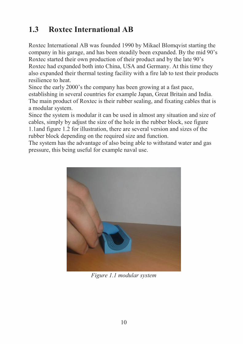
Roxtec International AB was founded 1990 by Mikael Blomqvist starting the company in his garage, and has been steadily been expanded. By the mid 90’s Roxtec started their own production of their product and by the late 90’s Roxtec had expanded both into China, USA and Germany. At this time they also expanded their thermal testing facility with a fire lab to test their products resilience to heat. Since the early 2000’s the company has been growing at a fast pace, establishing in several countries for example Japan, Great Britain and India. The main product of Roxtec is their rubber sealing, and fixating cables that is a modular system. Since the system is modular it can be used in almost any situation and size of cables, simply by adjust the size of the hole in the rubber block, see figure 1.1and figure 1.2 for illustration, there are several version and sizes of the rubber block depending on the required size and function. The system has the advantage of also being able to withstand water and gas pressure, this being useful for example naval use.

Figure 1.1 modular system

11

Figure 1.2 modular system

The product is installed in a socked and later pressed down to create a pressure and sealing the socked.

In figure 1.3an example of Roxtecs product modeled for practical use, in this case a steel frame (grey) with several rubber blocks (blue), although each individual block is not visible (the squares are the finite elements displaced). There is also another block (not focus of this thesis, therefore no details other than it applies the force needed) at the top, which with an internal contraption expands and is able to expand itself and put a force on the other blocks (in figure 1.3 represented by the arrows).

This force will compress the blocks and make the installation airtight, this is a typical product from Roxtec. There might be different shapes of the installation, but most builds on the same principle.

These are: A fixed frame (often made of steel), that are implemented in a wall or in the desired surface, using mortar or some other suitable method.

12

Placing the rubber blocks (for example 4x4 block in a square frame) in the frame, using a lube (usually grease) to minimize the friction between the blocks and the frame, after every two layer of rubber blocks it is recommended (if the frame allows) to have a steel plateau that stabilize the blocks and keep them from being pushed from the frame when the force is applied.

Inserting the special block that is able to expand and then apply the force, there are some models when the special block is circular and the blocks inserted in the middle to be able to be able to have the cable passing through the frame.

Apply the force, and wait for the grease to settle (usually 24 hours), after these hours the installation is ready to be used and withstand the internal/external pressure each model of the installation is made for.

Figure 1.3 several blocks in a frame with finite element generated

13

A finished installation might look like figure 1.4.

Figure 1.4 Installation with cables

To get a deeper understanding of the material that Roxtec is currently using, several tests are made, using a compressing machine seen in figure 1.5.

Test that yield experimental data for Roxtec, and data that is crucial for this thesis.

14

Figure 1.5 compressions test

15

2 Method

2.1 Theory and model building

This master thesis is focusing on improving the knowledge of hyperelastic material methods, and the implementations at Roxtec in Karlskrona. It started as a model development to find a method to simulate the contact between steel and rubber but changed into finding an appropriate way to simulate the rubber material Roxtec uses. 2.2 Target audience

This thesis will be published for the public to read, this due to only minor information of the material that Roxtec has provided. The target audience at Roxtec is the Product Development and Engineering department, who are more interested of knowing how to implement the hyperelastic material method, than to understand how it works. This leads to the formulas in this thesis will be generalized and not explaining in full detail how they works. 2.3 Moments in process

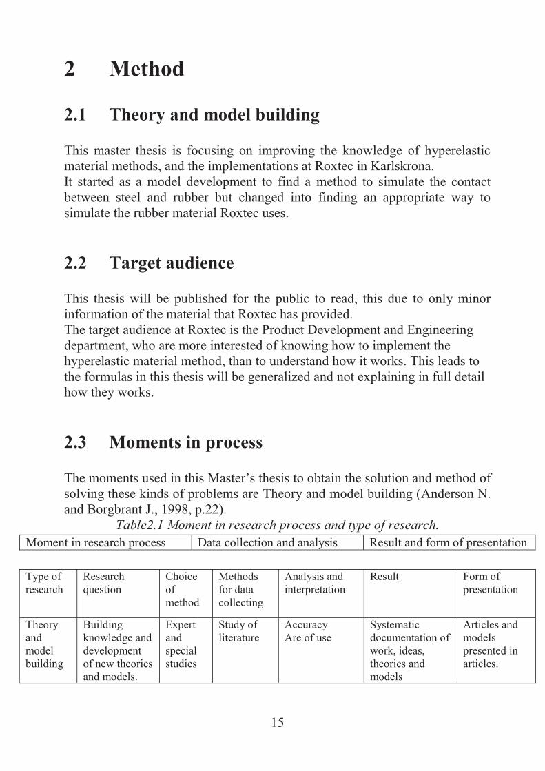
The moments used in this Master’s thesis to obtain the solution and method of solving these kinds of problems are Theory and model building (Anderson N. and Borgbrant J., 1998, p.22).

Table2.1 Moment in research process and type of research.

Moment in research process Data collection and analysis Result and form of presentation

Type of research

Research question

Choice of method

Methods for data collecting

Analysis and interpretation

Result Form of presentation

Theory and model building

Building knowledge and development of new theories and models.

Expert and special studies

Study of literature

Accuracy Are of use

Systematic documentation of work, ideas, theories and models

Articles and models presented in articles.

16

Their works were originally meant for the building industry, but can easily be used in other sectors as well, this due to the method of research they created. The table 2.1 explains the process of this thesis quite well and has been used during the process of obtaining and interprets the information. The work done on this thesis has been following the table accordantly: 2.3.1 Choice of method

After some meetings with Jörgen Landqvist and Dr. Johan Wall the choice was made. 2.3.2 Methods for collecting data

There were some extended studies of literature, this mostly due to being problematic to find good literature.

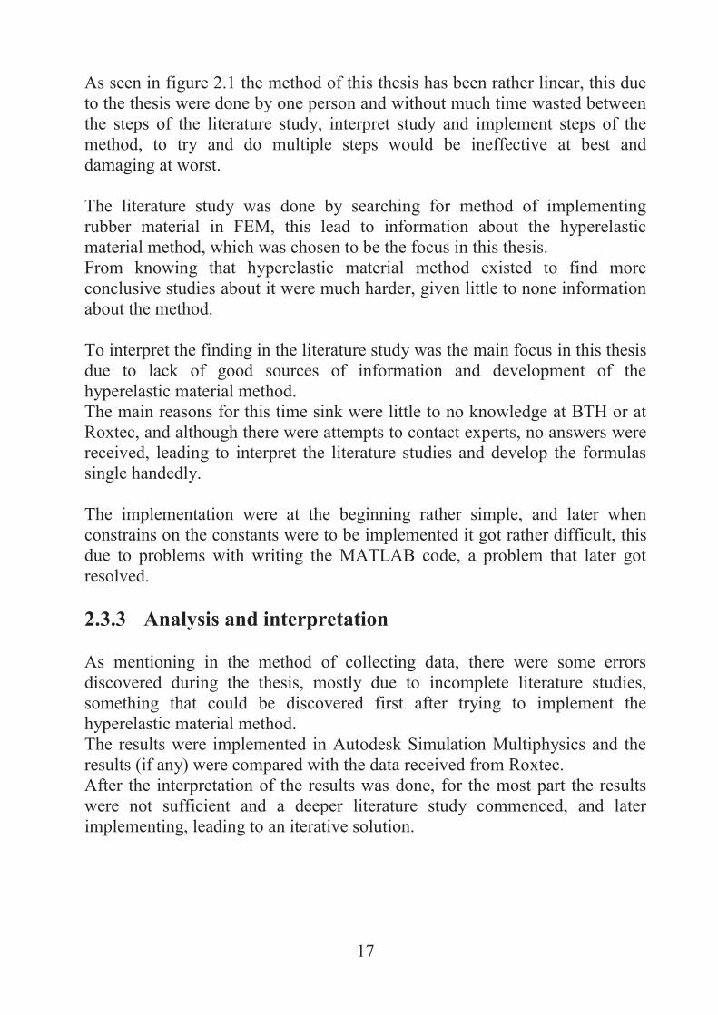
Figure 2.1 method and time spent

17

As seen in figure 2.1 the method of this thesis has been rather linear, this due to the thesis were done by one person and without much time wasted between the steps of the literature study, interpret study and implement steps of the method, to try and do multiple steps would be ineffective at best and damaging at worst. The literature study was done by searching for method of implementing rubber material in FEM, this lead to information about the hyperelastic material method, which was chosen to be the focus in this thesis. From knowing that hyperelastic material method existed to find more conclusive studies about it were much harder, given little to none information about the method. To interpret the finding in the literature study was the main focus in this thesis due to lack of good sources of information and development of the hyperelastic material method. The main reasons for this time sink were little to no knowledge at BTH or at Roxtec, and although there were attempts to contact experts, no answers were received, leading to interpret the literature studies and develop the formulas single handedly. The implementation were at the beginning rather simple, and later when constrains on the constants were to be implemented it got rather difficult, this due to problems with writing the MATLAB code, a problem that later got resolved.

2.3.3 Analysis and interpretation

As mentioning in the method of collecting data, there were some errors discovered during the thesis, mostly due to incomplete literature studies, something that could be discovered first after trying to implement the hyperelastic material method. The results were implemented in Autodesk Simulation Multiphysics and the results (if any) were compared with the data received from Roxtec. After the interpretation of the results was done, for the most part the results were not sufficient and a deeper literature study commenced, and later implementing, leading to an iterative solution.

18

2.3.4 Results

During the process of this entire thesis data and discoveries has been documented by hand, and later been documented and rewritten in this report. The result has also been verified by comparing the simulated result with the experimental data obtained from Roxtec. 2.3.5 Presentation

The results of this work are presented in this thesis as well as a presentation made in PowerPoint. Due to the implementation is important to Roxtec rather than the complete report, a scaled down version of the thesis for Roxtec, containing mostly just the theory, method and result. 2.4 Delimitation

Due to problems in finding information about the hyperelastic material method as well as the changing focus of the thesis leads to a thesis that only scratch the surface of the problem. There were tries to contact more experience people to ask about the different hyperelastic material models, but there were little to no response from this and therefore had to do most by myself. There were also little to no experience with the hyperelastic material method at Roxtec or at BTH according to Dr. Johan Wall at BTH and Jörgen Landqvist at Roxtec. Due to these problems the thesis can easily be continued and be the starting ground for another thesis in the future, due to the sheer volume of the problem. In this thesis only the hyperelastic material model called Mooney-Rivlin has been investigated, due to limitation in time. This material model is only one of several and the other can be investigated in future thesis, also implementation more than the most simple model has not been done, this also due to problems with the method as well as limited time. The material is also considered to be completely incompressible, this to simplify the expression in the hyperelastic material model. After talking to Jörgen Landqvist at Roxtec he confirmed that the material can be considered incompressible or near incompressible.

19

After discussions with Jörgen Landqvist at Roxtec, an approximation of the normal strain during real life situations is , and is the area that the thesis has been concentrated on mostly. Lastly there will be some censoring in the public version of this thesis, this due to it is necessary to use experimental data for the hyperelastic material methods. Experimental data that is important for Roxtec to protect.

3 Experimental data

To use the hyperelastic material method, experimental data is required to implement it properly (Tod Dalrymple, Jaehwan Choi, Kurt Miller, (2007), p6). The experimental data is obtained by a uniaxial test i.e. either an compression or an extension test, due to the characteristics Roxtecs products and installations an compression test is considered in this thesis, but an extension test is treated using the same methods. First, measurements on the testing piece needs to be done to determine the size and volume of the testing piece, important to know to later determine the strain, engineering stress and true stress, important components in the hyperelastic material method. Secondly the experiment is needed to be conducted, using in this case a compressing machine see figure 3.1. The machine is able to obtain the force it compress with, as well as the compression, this is also required to obtain strain, engineering stress and true stress.

20

Figure 3.1 compression test

To calculate the strain, engineering stress and true stress the following calculations has been made for the experimental data obtained from the machine i.e. the force and the displacement the force results in. The strain:

(3.1) The engineering stress:

(3.2) The true stress:

(3.3) In this thesis the area is assumed be constant in the tested part, this to simplify the calculations. Since the material is assumed to be incompressible the volume is not changing leading to the area is calculated as:

(3.4) (3.5)

Furthermore is to be assumed true stress unless other is stated.

21

4 Hyperelastic material method

4.1 Definition of a hyperelastic material

A hyperelastic materials different from other materials due to they are non-linearly elastic, isotropic and strain-rate independent (Autodesk section3 Module, 2011, p4). A hyperelastic material is also still elastic, meaning that it will return to its original form after the forces that is affecting the material is removed (Roland Jakel, (2010), p9). This is true even if the deformation is following the stress-strain curve in figure 4.1.

Figure 4.1 example of stress-strain curve.

A hyperelastic material is has little to no volume change during a deformation, this due to straightening the cross-linked molecular chains (Ansys, hyperelasticity, p3). A hyperelastic material can undergo and recover from large deformations on the order of 100-700% (Ansys, hyperelasticity, p3), it can be compared to the deformation of stainless steel is between 22-65% (Kim JR Rasmussen, Full-range Stress-strain Curves for Stainless Steel Alloys, p10) before breaking. As a final note: elastomers (like rubbers) are often modeled as hyperelastic materials (Roland Jakel, (2010), p10).

22

4.2 Background

The theory behind the hyperelastic material methods is based on a strain energy function U, which can be seen as a function based on the strain potential strain function. The elastic material properties are determent by the function U, which is the strain energy per volumes unit for any given materials (Per-Erik Austrell, 2001, p.15). This thesis and specially the theoretical part about hyperelastic material method led to an extensive literature study about the hyperelastic material method. This became an iterative process due to the curve-fit function in Autodesk Simulation Multiphysics are not working properly at all time, giving bad results as well as inconsistent values of the constants. For examples: they can give constants that cause the simulation to break after only a few iterations, extremely small or large deformations (compared to experimental data).

4.3 Different methods

In hyperelastic material methods there are several different methods to choose from, here will be a short description of the major methods. All information is gathered from A Review of Constitutive Models for Rubber-Like Materials by Aidy Ali, M. Hosseini and B.B. Sahari. 4.3.1 Different methods

Polynomial model This is usually used in modeling the stress-strain behavior of filled elastomers (rubber) (Per-Erik Austrell, (1997) , MODELING OF ELASTICITY AND DAMPING FOR FILLED ELASTOMERS, p1).

(4.1) Ogden

23

This is a standard method and one of the more commonly used hyperelastic material methods, and is used more than the Polynomial model and is also computationally more intensive, than the Polynomial model.

(4.2) Neo-Hookean This is a simpler version of the Ogden method and is also the simplest of the hyperelastic material methods, and is obtained by setting N=1 and =2 in the Ogden model.

(4.3) Yeoh This method is applicable for much wider range of deformation than most other hyperelastic methods, and is also able to predict behavior from data gained in uniaxial extension.

(4.4) Arruda and Boyce This model is applicable in the range of smaller strains, compare to the other methods.

(4.5) 4.4 Mooney-Rivlin

Mooney and Rivlin developed during the 1950’s the nonlinear elasticity theory for large deformation. Mooney developed a special material model which Rivlin later developed a general theory based on an expression based in strain energy. The Mooney-Rivlin model were chosen due to be the focus of this thesis partly due to it is together with Ogden the most common model (Aidy Ali, M. Hosseini and B.B. Sahari, A Review of Constitutive Models for Rubber-Like Materials,p235), partly due to an extensive literature study pointed to the Mooney-Rivlin method, for example the simulation of the deformation of a rubber O-ring (Autodesk, Section3 Module 3, Nonlinear analysis: hyperelastic material analysis, p26), a problem that is rather similar to the

24

products of Roxtec. A final reason that it were chosen were that lots of literature studies gave minor hints that Mooney-Rivlin were the preferred method, but none of these were clear enough to be presented. Since the main focus of the thesis is the method called Mooney-Rivlin this part will be more in detail then the other hyperelastic material models. 4.5 Constants

4.5.1 Different order of constants

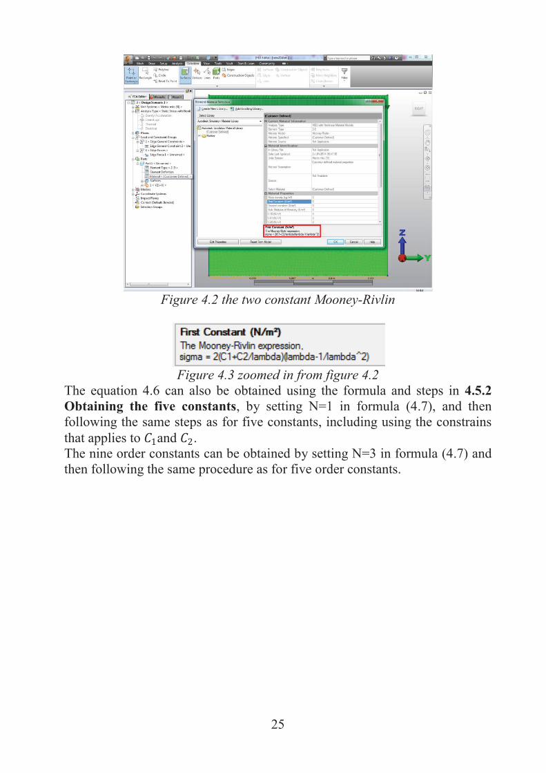
There are different orders of the Mooney-Rivlin method that can be implemented, all of these are different number of constants that are used to implement in a chosen software. The different orders are two, three, five and nine constant, the three constant orders are rarely used and are not possible to implement in Autodesk simulation Multiphysics, but there are other software programs that are supporting this. The higher order the more accurate stress-strain curve can be approximated, and therefore gives a better simulation. From figure 4.2, and showed in greater detail in figure 4.3 the equation is obtained:

(4.6)

25

Figure 4.2 the two constant Mooney-Rivlin

Figure 4.3 zoomed in from figure 4.2

The equation 4.6 can also be obtained using the formula and steps in 4.5.2 Obtaining the five constants, by setting N=1 in formula (4.7), and then following the same steps as for five constants, including using the constrains that applies to and . The nine order constants can be obtained by setting N=3 in formula (4.7) and then following the same procedure as for five order constants.

26

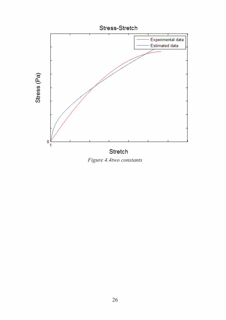
Figure 4.4two constants

27

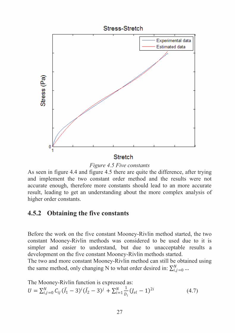
Figure 4.5 Five constants

As seen in figure 4.4 and figure 4.5 there are quite the difference, after trying and implement the two constant order method and the results were not accurate enough, therefore more constants should lead to an more accurate result, leading to get an understanding about the more complex analysis of higher order constants. 4.5.2 Obtaining the five constants

Before the work on the five constant Mooney-Rivlin method started, the two constant Mooney-Rivlin methods was considered to be used due to it is simpler and easier to understand, but due to unacceptable results a development on the five constant Mooney-Rivlin methods started. The two and more constant Mooney-Rivlin method can still be obtained using the same method, only changing N to what order desired in: The Mooney-Rivlin function is expressed as:

(4.7)

28

(Aidy Ali, M. Hosseini, B.B. Sahari, 2010, p.234) Trying to obtain the five Mooney-Rivlin methods, by setting N=2.

(4.8) Were =0 and due to incompressible material =1. Since it is the five constant Mooney-Rivlin that is interesting the function is:

(4.9) The three invariants have the following properties (Aidy Ali, M. Hosseini, B.B. Sahari, 2010, p.233):

(4.10) (4.11)

(4.12) Since the material is incompressible , this leads to (R. S. Rivlin, 1947, p.387)

(4.13) The invariants have now the following properties:

(4.14)

(4.15) To be able to obtain the constants that define our function a redefining of the function W is needed. Since , were i is the different axis (R. S. Rivlin, 1947, p.389).

(4.16)

(4.17) This due to , for it is a uniaxial test. To get the stress function a derivation is necessary, and since the invariant is still difficult to obtain, a multiplication with is necessary (R. S. Rivlin, 1947, p.389).

(4.18)

(4.19)

29

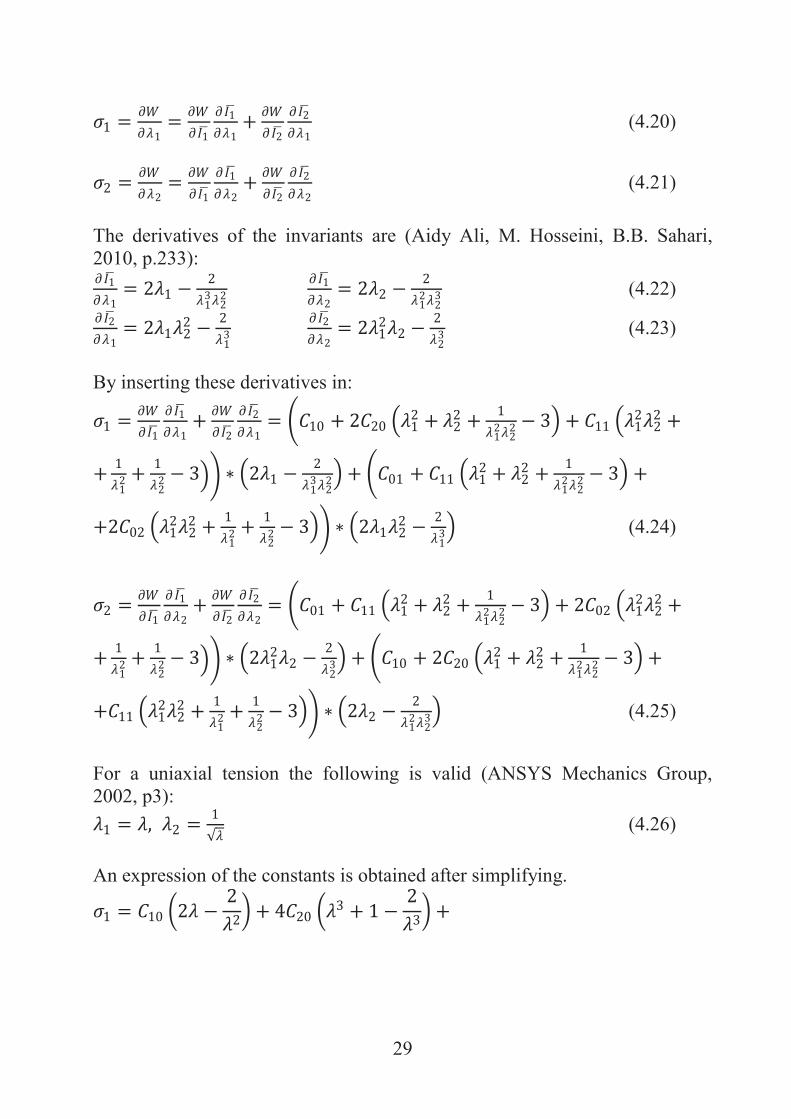
(4.20)

(4.21)

The derivatives of the invariants are (Aidy Ali, M. Hosseini, B.B. Sahari, 2010, p.233):

(4.22)

(4.23) By inserting these derivatives in:

(4.24)

(4.25)

For a uniaxial tension the following is valid (ANSYS Mechanics Group, 2002, p3):

(4.26) An expression of the constants is obtained after simplifying.

30

(4.27)

(4.28) Adding these two expressions to obtain the final expression of the constants needing to describe the material properties.

(4.29) To obtain the different constants, a curve fit of the expression against the experimental data is required. There is also some constrains needed to be accounting for when doing the curve fit (ANSYS INC, (2009), Theory Reference for the Mechanical APDL and -mechanical Applications) (G.I Barenblatt, D.D. Joseph, (1996), The Complete Bibliography of the publications of R.S. Rivlin vol I), they are:

(4.30) (4.31)

At last there is the bulk modulus to calculate, since its uniaxial data that is relevant only the first bulk modulus is of importance and can be calculated by.

(4.32) With data provided by Roxtec International AB the poisons ratio is estimated to be . 4.6 Numerical estimation of the constant

In this thesis the program MATLAB has been chosen to do the numerical estimation of the five constants. To be able to estimate the best constant that fits the curve-fit, a program were written, to insure that the results is as good as possible the program is created as an optimization solver. Where there are some inputs, the experimental data and the constrains, in order to estimate how close to the curve the estimated constants are an RMS (Root Mean Square) function were created, this to try and minimize the errors of the problem.

31

To obtain the Mooney-Rivlin constants, run the MATLAB code found in the appendix called Main, together with the two functions needed: calcRMS and mycon2. 4.7 Potential warning

There might be some problems with the constants when trying to implement the constants, for example an occurring problem was , which cause some problems in the implementation in Autodesk Simulation Multiphysics. In other words, when the constants are or almost are at the extreme boundaries. Another example is when , or the constants are almost at their recommended maximum/minimum values being as stated when trying to implement a constant with greater value in Autodesk Simulation Multiphysics. One possible way round this was to define and , using this has shown improvement in the simulation of FEM, instead of aborting the simulation, or get invalid results. Other smaller change to avoid the extreme case for example

might be necessary to be able to obtain good and valid constants. These smaller changes that needs to be done can differ in so many ways and can abort a simulation, and the solution is unique for every case, therefore only giving some examples and possible improvements. It is important to know that these things might be problematic if trying to obtain some material constants and should be acknowledged.

5 Implementing in FEA

The function and constants are not for much use if they are not implemented in a FEA program that knows how to handle the hyperelastic material method, since Roxtec uses Autodesk Simulation Multiphysics it is the main focus of implementation. 5.1 Autodesk Simulation Multiphysics

The implementation of the Mooney-Rivlin method in Autodesk Simulation Multiphysics is rather simple.

32

In this case a simple 2D model is chosen to simulate the Mooney-Rivlin method. First a model is created, in this case a rectangular shape, se figure 5.1. In case of a 2-D model the element type 2-D element is preferable (Autodesk, (2011), Nonlinear analysis: hyperelastic material analysis, p31) and in the case of a 3-D model brick element is preferable (Anders Pettersson, (2000), p29).

Figure 5.1 simple 2D models

There must be boundary conditions and a force in order to keep the equilibrium of this block that is created, during simulations during the work of this thesis there were very little difference in displacement if the block were fixated in both Y and Z axial, or just Z axial. To apply the force F it is simply to add it at the top of the block, if the block is fixated in both axial directions there should be a boundary condition that keeps the top part of the block to displace in Y direction as well. This to simulate a compression test, se figure 1.5, although not visible in that figure the block deforms and gets a rounded edge, as suspected if there would be boundary conditions preventing the top and bottom part to deform in Y direction.

33

Many FEA software's has the option of creating an automated mesh, were the two most important factors is Mesh Density, and Mesh Size, both is used to determine how fine or coarse the mesh is in the model se figure 5.2.

Figure 5.2 mesh

Since the Mooney-Rivlin is an energy based method, it is simply to define in the program that it is a hyperelastic material method, in this case Mooney-Rivlin, se figure 5.3.

34

Figure 5.3choices of material properties

After defining the hyperelastic material method, add the material constants

into the material section, se figure5.4 and figure 5.5.

Figure 5.4 the material constants

35

Figure 5.5 the material constants

5.2 Potential warning

There might be problem of simulating the model if there are too few time steps se figure 5.6, since hyperelastic materials are very nonlinear it is required to use small time steps (Autodesk, (2011), Nonlinear analysis: hyperelastic material analysis, p36), suggesting around 1 000 steps.

36

Figure 5.6 analysis parameter, the time step

There can also be problems if the mesh is not fine enough for the simulation, a finer mesh can solve this problem. Lastly, there might be certain times when the simulation aborts due to the system might be under defined. Adding additional boundary conditions might solve this issue. The method should also be applicable in more complex simulations, simply by defining each part of the models with the given constants. 5.3 Verifying the results

The results of the FEM is quite easy to verify this due to experimental data obtained from Roxtec, simply make the model either has an force that is similar to one that is in the experimental data and analyze the model, if the time steps has been chosen for example 1 000 steps, and the load is increasing linear (if not changed, which is not recommended) relative easy to know the load for each time step. The simulation shown in figure 5.7 is made with the force F=9kN, and has a displacement of 5.3mm. The choice of the force of F = 9kN were made due to

37

that the maximum measured force were equal to 9 454N. Rounded down to an "easy" number would be 9,5kN but this was considered too close to the highest measured value. When compare with the experimental data the displacement is 8.4mm, also shown in figure 5.8.

Figure 5.7 deformed block

38

Figure 5.8 experimental test force vs displacement curve

At first glance it might not seem as a good result, but at Roxtec the normal deformation is When the simulation has the deformation, for example when the force F=4.5kN has an displacement of 3.8mm, which if compared with the experimental data has an displacement of 3.64mm where the deformation is , this is for the upper part of the normal deformation. The reason the constants obtained were estimated with deformations not in the usual area of deformation for Roxtec were to try and make a general estimation, for a greater range than is necessary in case it is needed.

6 Results

The result is the steps needed to take to obtain the Mooney-Rivlin constants and later implement these in FEA software. First make obtain the experimental data needed, by performing an compression test or an extension test.

39

Convert the data into true stress/strain, and implement them in the numerical estimation, to obtain the constants. Finally an implementation of these constants in a FEA software is needed to simulate the given material. An example is given using the material known as Roxylon using experimental data acquired Roxtec. By using the data in the numerical solution (in this case MATLAB) the following constants were obtained:

By using these constants in a 2D model in the chosen FEA software (in this case Autodesk Simulation Multiphysics), the total displacement were 6.3mm for a force of 9kN for illustration se figure 6.1

Figure 6.1 displacement

40

7 Summary and discussion

7.1 Summary

There is problems trying to simulate rubber in FEA software partly due to the material properties of rubber is more complex than for example steel, due to the relative small portion of productive industry works with rubber, therefore leads to only small improvements over time. While this thesis has looked at the hyperelastic material method to make the simulations more reliable and more accurate than what Roxtec is currently using, the results show that at least with simple models there is clearly use for hyperelastic material method to try and implement the method in more complex problems. 7.2 Economic, social, ethical and ecological progress

The results of this thesis will hopefully mean that Roxtec can better simulate their materials and continue to develop their products. Increase accuracy in simulations will lead to a decrease in experimental testing, due to the cheaper and easier simulations of the given materials as well. It will also lead to more complex simulations being completed with greater chance of an accurate result, meaning that a deeper understanding about the material and its interactions will develop. A better simulation will also lead to a more secure environment in which the Roxtec install their product, such as gas or liquid heavy environment, meaning that it minimizing the risk (although small to begin with) for the people installing at. As mentioning earlier an increase in simulations leads to a decrease in experimental testing, and therefore minimizing the material used and later discarded. Even the simulation is depended on experimental data, this will lead to an initial experimental testing to receive the information needed for the simulation, therefore leading in the long run to a decrease in wasted material. This thesis is for the most part a theoretical thesis, having little to no impact directly on ethical aspects of Roxtec, in the long run it may reduce the need for wasted material, as mentioning above due to a reduction of experimental testing. A reduction that may lead to reduction in the necessary product needed to produce the rubber, for example oil and natural rubber.

41

A reduction of oil and natural rubber needed for the production of the different rubbers Roxtec is using, may lead to a more sustainable society and environment due to not being forced to expand plantations and oil production. 7.3 Discussion

This thesis has been a great learning experience and learned especially that if a problem seems easy it is rarely are. The struggle has been mostly trying to find sufficient literature to study and to interpret, due to the rather badly written sources that were found either assumed that the reader knew almost everything there is about the hyperelastic material method or it will not tech one anything. Great efforts were made trying to collect as much information about the Mooney-Rivlin method one could find and trying to put everything in one place, this thesis. There were studies of many different literatures all could be useful, but only a handful proved to be useful. Since there were only a few good literature studies available a lot of time has been spend on trying to understand and almost reinvent the method as well as implement the method in MATLAB, this was a large time sink. Since this is mostly a theoretical thesis and therefore has some problems meeting certain criteria that are necessary for a master thesis for example be able to develop products, processes and systems with respect to people’s backgrounds and need for an economic, social and ecologic sustainable development. Most of these difficult criteria’s has been discussed in section 7.2 economic, social, ethical and ecological progress, and might be seen out of place because of this.

In the end, the result presented is the tools needed to implement rubber materials in FEA software, but the time needed to “reinvent the wheel” can’t really be shown in the report therefore it became a rather short thesis.

42

7.4 Continuation

The thesis has big potential to have another thesis building upon this, for example look at other hyperelastic material models and how they will work with the material Roxtec is using. Another suggestion is to continue with the Mooney-Rivlin method and simulate more complex structures, and how it interacts with for example steel or friction. A third alternative could be to try and simulate other material with the hyperelastic material method to investigate if it can be useful in other areas other than some rubbers.

43

8 References

1. NicolasAnderson, Jan Borgbrant, (1998), Byggforskning – processer och vetenskaplighet, Institutionen för Väg och Vattenbyggnad, Luleå tekniska universitet.

2. Per-Erik Austrell, (2001), KONSTRUKTIONSBERÄKNINGAR FÖR GUMMIKOMPONENTER, Structural mechanics LTH.

3. Aidy Ali, M. Hosseini, B.B. Sahari, (2010),A Review of Constitutive Models for Rubber-Like Materials, Department of mechanical and manufacturing Engineering, Faculty of Engineering, University Putra Malaysia

4. R. S. Rivlin, (1947), LARGE ELASTIC DEFORMATION OF ISOTROPIC MATERIALS IV. FURTHER DEVELOPMENTS OF THE FENERAL THEORY, Philosophical Transactions of the Royal Society of London. Series A, Mathematical and Physical Sciences

5. Autodesk, (2011), Section3 Module 3, Nonlinear analysis: hyperelastic material analysis

http://webcache.googleusercontent.com/search?q=cache:jCgyp3q-ZysJ:studentsdownload.autodesk.com/ef/27288/cdcoll/downloads/CAEproject/CAEproject_Section3/CAEproject_Section3_Module3/Section3_Module3_Hyperelastic.pptx+&cd=1&hl=sv&ct=clnk&gl=se

6. Ansys, Module, Hyperelasticity

http://ansys.net/ansys/papers/nonlinear/conflong_hyperel.pdf

7. Dr.-Ing. Roland Jakel, (2010), Analysis of Hyperelastic Materials with MECHANICA – Theory and Application Examples –,Chemnitz University of Technology

8. Tore Dahlberg, (2010), Teknisk hållfastighetslära, Studentliteratur AB, Lund

9. Kim JR Rasmussen, (2001), Full-range Stress-strain Curves for Stainless Steel Alloys, The University of Sydney Department of Civil Engineering

10. Ansys Mechanics Group, (2002), ANSYS material modeling: Hyperelastic material characterization, ANSYS Inc

44

http://ansys.net/ansys/papers/nonlinear/hyper_elasticcity_curvefitting.pdf

11. Anders Pettersson, (2000), FINITE ELEMENT MODELLINGOF A RUBBER BLOCKEXPOSED TO SHOCK LOADING, Solid Mechanics & Structural Mechanics, LTH

12. Tod Dalrymple, Jaehwan Choi, Kurt Miller, (2007), ELASTOMER RATE-DEPENDENCE: A TESTING AND MATERIAL, MODELING METHODOLOGY, DASSAULT SYSTÈMES SIMULIA CORP

13. Per-Erik Austrell, (1997) , MODELING OF ELASTICITY AND DAMPING FOR FILLED ELASTOMERS, Lund institute of technology, Lund Universitet.

14. ANSYS INC, (2009), Theory Reference for the Mechanical APDL and -mechanical Applications, ANSYS INC.

http://orange.engr.ucdavis.edu/Documentation12.0/120/ans_thry.pd

15. G.I Barenblatt, D.D. Joseph, (1996), The Complete Bibligraphy of the publications of R.S. Rivlin vol I, University of Cambridge, University of Minnesota

45

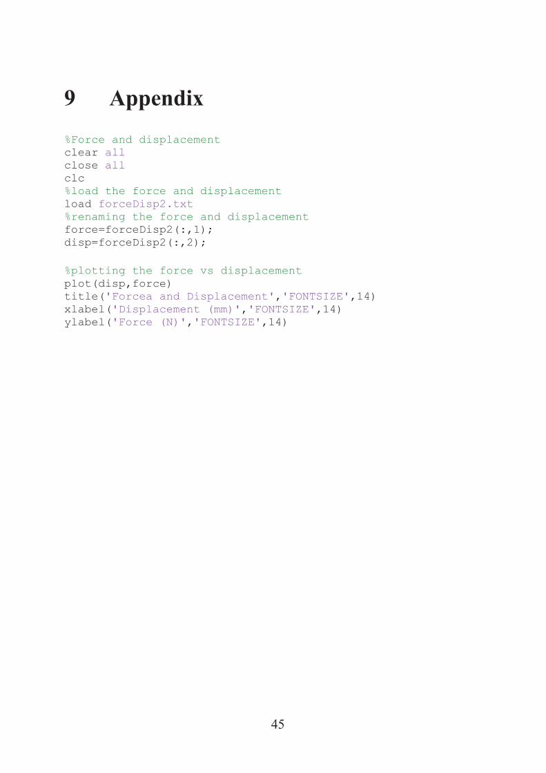
9 Appendix %Force and displacement clear all close all clc %load the force and displacement load forceDisp2.txt %renaming the force and displacement force=forceDisp2(:,1); disp=forceDisp2(:,2); %plotting the force vs displacement plot(disp,force) title('Forcea and Displacement','FONTSIZE',14) xlabel('Displacement (mm)','FONTSIZE',14) ylabel('Force (N)','FONTSIZE',14)

46

%Main clear all close all clc %loading all of the obtained test results. load test4.txt load engStress.txt load TrueStressStrain.txt %renaming the data eStress=engStress(:,1); %engineering stress Strain=test4(:,2); Stress=test4(:,3); Stress2=TrueStressStrain(:,1); Strain2=TrueStressStrain(:,2); Stretch=Strain2+1; %lambda %Defineing the maximum and minimum values of the constants, given by %Aurodesk (if the value is over 10^8, a warning appears) c10_min = -1*10^8; c10_max = 10^8; c01_min = -1*10^8; c01_max = 10^8; c20_min = -1*10^8; c20_max = 10^8; c11_min = -1*10^8; c11_max = 10^8; c02_min = -1*10^8; c02_max = 10^8; %starting guess, usally in the middle. x0 = [(c10_min+c10_max)/2 (c01_min+c01_max)/2 (c02_min+c02_max)/2 (c11_min+c11_max)/2 (c20_min+c20_max)/2]; lb_old=[c10_min c01_min c20_min c11_min c02_min]; ub_old=[c10_max c01_max c20_max c11_max c02_max]; %starting to find the five different constants. options = optimoptions(@fmincon,'Algorithm','interior-point' , 'display', 'iter', 'TolX',1E-99,'TolFun',1E-9,'DiffMinChange',1E-6); [x, fval, exitflag, output] = fmincon('calcRMS', x0', [], [], [], [], lb_old, ub_old, 'mycon2', options); x %displaying the results K=2*(x(1)+x(2))/(0.1) %plotting a smaller range of the calculated function and the experimental %values Stretch2=Stretch(1:269); plot(Stretch2, eStress(1:269)) hold on;

47

plot(Stretch2, (x(1)*(2*Stretch2-(2*Stretch2.^-2))+x(2)*(2-2*Stretch2.^-3)+x(3)*4*(Stretch2.^3+1-2*Stretch2.^-3)+x(4)*2*(3*Stretch2.^2-1+Stretch2.^-1-Stretch2.^-3-2*Stretch2.^-4)+x(5)*4*(2*Stretch2-Stretch2.^-2-Stretch2.^-5)),'r') title('Force and Displacement','FONTSIZE',14) xlabel('Displacement (mm)','FONTSIZE',14) ylabel('Force (N)','FONTSIZE',14) %plotting the calculated function and the measured values. figure; plot(Stretch, eStress) hold on; plot(Stretch,(x(1)*(2*Stretch-(2*Stretch.^-2))+x(2)*(2-2*Stretch.^-3)+x(3)*4*(Stretch.^3+1-2*Stretch.^-3)+x(4)*2*(3*Stretch.^2-1+Stretch.^-1-Stretch.^-3-2*Stretch.^-4)+x(5)*4*(2*Stretch-Stretch.^-2-Stretch.^-5)),'r') title('Force and Displacement','FONTSIZE',14) xlabel('Displacement (mm)','FONTSIZE',14) ylabel('Force (N)','FONTSIZE',14) %plotting from -1 to 2 to show how the calculated function looks like. figure; plot(Stretch, eStress) hold on; Stretch2=-1:3/1345:2; %setting the x-axis to a wider range to expand the view. plot(Stretch2,(x(1)*(2*Stretch2-(2*Stretch2.^-2))+x(2)*(2-2*Stretch2.^-3)+x(3)*4*(Stretch2.^3+1-2*Stretch2.^-3)+x(4)*2*(3*Stretch2.^2-1+Stretch2.^-1-Stretch2.^-3-2*Stretch2.^-4)+x(5)*4*(2*Stretch2-Stretch2.^-2-Stretch2.^-5)),'r') title('Force and Displacement','FONTSIZE',14) xlabel('Displacement (mm)','FONTSIZE',14) ylabel('Force (N)','FONTSIZE',14)

48

function [c,ceq] = mycon2(x) %in A[C10 C01 C20 C11 C02; C10 C01....] to set an constrain ex C10>0 % [-1 0 0 0 0] or C20+C11+C02>0 [0 0 -1 -1 -1], where an positive 1 is % equal or less than zero. A=[-1 -1 0 0 0; 0 0 -1 0 0; 0 0 0 0 1; 0 0 -1 -1 -1]; %During a case C10=-C01 I needed to set both C10 and C01 to be greater than %0 in addition to the other constrains. % A=[-1 -1 0 0 0; 0 0 -1 0 0; 0 0 0 0 1; 0 0 -1 -1 -1;-1 0 0 0 0;0 -1 0 0 0]; c=A*x; ceq=0;

49

function Diff = calcRMS(x) %UNTITLED4 Summary of this function goes here % Detailed explanation goes here load test4.txt load engStress.txt load TrueStressStrain.txt %renaming the data eStress=engStress(:,1); Strain=test4(:,2); Stress=test4(:,3); Stress2=TrueStressStrain(:,1); Strain2=TrueStressStrain(:,2); Stretch=Strain2+1; %lambda % % tried a smaller range of data to calculate the inital values. % Stress2=Stress2(1:900); % Stretch=Stretch(1:900); %calculate an approximative stress function. StressCalc=(x(1)*(2*Stretch-(2*Stretch.^-2))+x(2)*(2-2*Stretch.^-3)+x(3)*4*(Stretch.^3+1-2*Stretch.^-3)+x(4)*2*(3*Stretch.^2-1+Stretch.^-1-Stretch.^-3-2*Stretch.^-4)+x(5)*4*(2*Stretch-Stretch.^-2-Stretch.^-5)); %setting the first node to origo due to hard constrain that is always true. StressCalc(1,1)=0; plot(StressCalc) %It is this rms function that the loop is trying to minimize to get a good %approximation of the constants. Diff=rms(eStress-StressCalc); end