Practical Challenges in Reserve Risk - Actuaries
36
October 2016 Practical Challenges in Reserve Risk Kevin Chan FCAS FCIA [email protected] Michael Ramyar FIA [email protected] Abstract This document describes the challenges experienced in quantifying reserve risk with practical solutions suggested. It provides a pragmatic development towards advancing the assessment of reserve risk. It is aimed at general insurance actuaries who want an understanding of the challenges encountered in reserve risk without becoming too engaged in the technical details which can often be a distraction to the underlying issues. However, owing to the nature of the subject, technical content is unavoidable and can be found in the appendices. The first part of this document is a review of the fundamental concepts of reserve risk while the second part provides readers with a deeper understanding of the challenges faced within practical implementation of reserve risk. The authors hope that this publication will generate discussions in the general insurance actuarial community prompting the development of a common best practice approach to reserve risk As such it is recommended that this document to be circulated to all practitioners involved in reserving and reserve risk. Keywords: reserving, reserve risk, stochastic reserving, bootstrap, Mack’s model
Transcript of Practical Challenges in Reserve Risk - Actuaries

October 2016
Practical Challenges in Reserve Risk
Kevin Chan FCAS FCIA
Michael Ramyar FIA
Abstract
This document describes the challenges experienced in quantifying reserve risk with practical solutions
suggested. It provides a pragmatic development towards advancing the assessment of reserve risk. It
is aimed at general insurance actuaries who want an understanding of the challenges encountered in
reserve risk without becoming too engaged in the technical details which can often be a distraction to
the underlying issues. However, owing to the nature of the subject, technical content is unavoidable
and can be found in the appendices.
The first part of this document is a review of the fundamental concepts of reserve risk while the second
part provides readers with a deeper understanding of the challenges faced within practical
implementation of reserve risk. The authors hope that this publication will generate discussions in the
general insurance actuarial community prompting the development of a common best practice
approach to reserve risk As such it is recommended that this document to be circulated to all
practitioners involved in reserving and reserve risk.
Keywords: reserving, reserve risk, stochastic reserving, bootstrap, Mack’s model

Practical Challenges in Reserve Risk
SECTION 0
Notes on Reproduction of this Document
The motivation of this document is to educate and encourage improvement of practices across the
general insurance industry in the assessment of reserve risk. As such the authors encourage this
document to be distributed freely but in its full original form. All constructive comments are welcomed
via email as provided above.
About the Authors
This document shares the personal views of both authors, Kevin Chan and Michael Ramyar, reflecting
their knowledge and research gathered in the field of reserve risk.
Kevin Chan has been a Fellow of the Casualty Actuarial Society since 2004. He has been with XL
Group for over 10 years, leading the reserve risk work stream since 2012. He has prior experience in
Casualty reserving and pricing, as well as consulting from PriceWaterhouseCoopers Toronto.
Michael Ramyar has been a Fellow of the Institute of Actuaries since 2011. He is an independent
consultant with a variety of experience more recently focusing on capital and reserve risk. He supported
the XL Group reserve risk team in research, training, validation and peer review.
Both Kevin and Michael have extensive knowledge of reserve risk, not only have they participated in
the Institute and Faculty of Actuaries (IFoA) Working Party on Pragmatics Stochastic Reserving, they
have presented at various conferences including plenary session titles “Alleviating Reserving Stress” at
the 2015 General Insurance Research Organising Committee (GIRO) conference.
Acknowledgements
Thanks to XL Group – in particular Susan Cross (Global Chief Actuary), Jean-Luc Allard (Head of
Insurance Actuarial Financial Reporting and Group Reporting) and Adrian Amiri (Lead on Solvency II
Technical Provisions and Reserve Risk) – for the resource provided in allowing the authors to conduct
research in the topic of reserve risk.
Thanks also to James Orr (Chair of IFoA Working Party on Pragmatics Stochastic Reserving) and
colleagues in XL Group (Paul Goodenough, Nutan Rajguru, and Ashwani Arora) for their review and
valuable input.
A special thanks to Sonya Chana, Krishna Rajah and Sonal Shah for providing extensive editing on this
document.

Practical Challenges in Reserve Risk
CONTENTS
SECTION 1 – INTRODUCTION........................................................................................... 1
SECTION 2 – A BRIEF TUTORIAL OF RESERVE RISK ............................................... 2
2.1 BASIC CONCEPTS OF RESERVE RISK ............................................................................................. 2
2.1.1 What is Reserve Risk? ............................................................................................................ 2
2.1.2 Models .................................................................................................................................... 3
2.1.3 Sources of Reserve Risk ......................................................................................................... 3
2.2 HOW TO ESTIMATE PREDICTION ERROR ....................................................................................... 3
2.2.1 Analytical approach ............................................................................................................... 4
2.2.2 Empirical approach ............................................................................................................... 5
SECTION 3 – PRACTICAL CHALLENGES ...................................................................... 6
3.1 INCONSISTENCY BETWEEN RESERVING AND RESERVE RISK ........................................................ 6
3.1.1 Inconsistencies in Data .......................................................................................................... 6
3.1.2 Inconsistencies in Model ........................................................................................................ 7
3.1.3 Inconsistencies in Parameters ............................................................................................... 8
3.1.4 The Scaling Issue ................................................................................................................... 8
3.1.5 Summary ................................................................................................................................ 9
3.2 COMMON MISCONCEPTIONS ....................................................................................................... 10
3.2.1 “The bootstrap model doesn’t work. We need a better model.” .......................................... 10
3.2.2 “Paid triangle should be used to estimates the reserve volatility” ..................................... 10
3.2.3 “We had a good year so why has the CoV increased?” ..................................................... 11
3.2.4 Is the CoV an absolute risk measure? .................................................................................. 12
3.2.5 Using the CoV directly from bootstraping an industry triangle .......................................... 12
3.2.6 Every triangle is unique! ...................................................................................................... 13
3.2.7 Uncertainty in the estimation of reserve risk ....................................................................... 13
3.2.8 Is using an underwriting year triangle appropriate? .......................................................... 14
3.2.9 Comparisons between underwriting risk and reserve risk CoV ........................................... 15
3.2.10 Dependency between lines of business ............................................................................... 15
3.2.11 Summary ............................................................................................................................ 16
3.3 OTHER PRACTICAL CHALLENGES ............................................................................................... 16
3.3.1 Netting down an aggregate gross distribution ..................................................................... 16
3.3.2 How much data is required .................................................................................................. 16
3.3.3 High sensitivity to changes in assumptions .......................................................................... 17
3.3.4 One-year time horizon ......................................................................................................... 17
SECTION 4 – CONCLUSION ............................................................................................. 18
APPENDIX A – HOW WRONG IS THE ESTIMATION OF RESERVE RISK? ......... 19
APPENDIX B – DIVERSIFICATION ADJUSTMENT .................................................... 29
APPENDIX C – “NETTING DOWN” A GROSS AGGREGATE DISTRIBUTION ..... 30
REFERENCES ....................................................................................................................... 33

Practical Challenges in Reserve Risk
1
SECTION 1 – INTRODUCTION
The move towards a risk-based capital environment and the ever changing regulatory environment has
meant that the quantification of reserve risk has become vital for the wider general insurance sector. In
response to this, over the recent past a considerable amount of research and development has already
taken place to better quantify reserve risk.
The authors firmly believe that all existing practices and knowledge should be consolidated so that
common generally accepted market practice guidance can be created for the present and future reserving
and reserve risk practitioners. This paper attempts to address this by providing an overview of the
common practical challenges faced and proposing possible solutions. Ideally, if stochastic reserving
techniques were more embedded by the wider market into the reserving process, the derivation of the
reserve uncertainty will have less challenges. However, the highly technical nature of stochastic
reserving has in many instances created a barrier for reserving actuaries and practitioners. As a
consequence, this has led to one of the biggest practical challenges of evaluating reserve risk which will
be explored in this document.
The remainder of this document is structured as follows:
Section 2 provides a brief tutorial of what reserve risk is and how it can be estimated. Not
only does this section cover basic terminologies and fundamental concepts used throughout
the document, it also serves as an educational piece to the topic of reserve risk.
Section 3 is the core of this document detailing practical challenges experienced in reserve
risk. Building on the basic concepts of reserve risk provided in the previous section, the
reader will be able to understand why these challenges exist. A clear understanding of the
cause of these challenges will allow practitioners to develop high-level solutions.
The challenges are categorised into the following three sub-sections with cross-references
provided throughout the document since most of the challenges are interlinked:
o Inconsistency between reserving and reserve risk allowing the reader to fully
understand the source of the most problematic issue; namely “scaling” the reserve
distribution mean to the best estimates of reserve.
o Common misconceptions are another major challenge creating obstacles in the
advancement of reserve risk. Providing clarity on these concepts and offering
potential solutions is a step to eliminating these issues. This sub-section also leads
to a theoretical study on “How wrong is our estimate of reserve risk” which is
outlined in detail in Appendix A.
o Other practical challenges include other issues relating to reserve risk that are
worth highlighting. Some of these are covered extensively in other literature
including the authors’ previous work.
Section 4 provides the conclusion, which summarises the salient points of discussion in this
document.
Please note that all suggested approaches should not be interpreted as the only approach but are intended
to initiate discussion for further development of a common industry wide generally accepted market
practice. A list of references including suggested further readings are indicated in square brackets
throughout the document which corresponds to the list in the Reference section.

Practical Challenges in Reserve Risk
2
SECTION 2 – A BRIEF TUTORIAL OF RESERVE RISK
2.1 Basic Concepts of Reserve Risk
Across the general insurance actuarial community there are large variations in the fundamental
understanding of what reserve risk is and what it is estimating. This issue is the most fundamental
challenges in embracing and advancing reserve risk market practices. The remainder of this section
aims to address this challenge.
2.1.1 What is Reserve Risk?
It is important to establish conventional terminology in order to describe the basic concept of reserve
risk. The required reserve is the payment ultimately be paid to settle all incurred claims. This value
can take on a range of possible outcome and can only be known with certainty when all claims have
been finally settle in the future. The estimated reserve is a point estimate of the average required
reserve resulted from reserving methodologies using parameters derived from historical data.
Reserve risk is the uncertainty in the estimation of the required reserve. It is related to the difference
between the required reserve and the estimated reserve. In an ideal world, if the true mean of the
required reserve is known, the estimated reserve would be set as the true mean and the reserve risk
would simply be quantified by the variance of the distribution of required reserve R:
𝑉𝑎𝑟(𝑅) = 𝐸[(𝑅 − 𝐸(𝑅))2]
The variance measures the volatility of a random process by taking the average of the squared error
between all possible outcome and the true mean outcome. The standard deviation is the square root of
this quantity.
The term prediction error arises because within the well-known variance definition, the true mean
outcome, E(R) is actually unknown. In practice, E(R) is replaced by an estimate �̂�. Thus the result is a
mean square error of prediction (MSEP), not a variance, and the square root is not a standard deviation
but a prediction error. The definition is as follows:
𝑀𝑆𝐸𝑃(�̂�) = 𝐸[(𝑅 − �̂�)2| 𝐷] (2.1.1)
The MSEP is conditioned on data D because data is needed to derive parameters of a selected model
that in turn are used to calculate �̂�. The reader is encouraged to compare and contrast the similarities
and differences, term by term, of MSEP versus variance. Take careful note of the “hats”, these signify
a deterministic point estimate, rather than the random variable.
With some arithmetic work, the MSEP can be broken down into two components:
𝑀𝑆𝐸𝑃(�̂�) = 𝑉𝑎𝑟[𝑅|𝐷] + (�̂� − 𝐸(𝑅| 𝐷))2 (2.1.2)
The first term is related to the process risk, the uncertainty arises from the difference between all
possible required reserve and the true mean required reserve, and the second term is related to the
parameter error, the difference between the estimated reserve and the true mean required reserve.
These correspond to the two sources of reserve risk. Note that once an estimate �̂� is made, the second
term is a fixed constant hence termed “parameter error” instead of “parameter risk” for the rest of this
paper.
Practical Challenges in Reserve Risk
3
Now, the difference between the standard deviation and prediction error is clear. The prediction error
not only has captured the intrinsic uncertainty of a random process around the true mean, but also the
error in estimating the true mean. These sources of error are further discussed below.
2.1.2 Models
In order to quantify the prediction error of reserve, a model is specified. It is impossible for any
mathematical model to capture the full multitude of factors of the real underlying process. A model is
a simplification of reality whilst reflecting the significant dynamics. In reserving context, regardless of
how complex the reserving methodology is, it will not fully reflect the reality. In terms of reserve risk,
since the prediction error of reserve relates to both the required reserve (𝑅) and the estimated reserve
(�̂�), the error in model specification is not only related to how good the model reflects reality, but also
how consistent the model is with the reserving process. This point will be further examined in Section
3.1.4.
2.1.3 Sources of Reserve Risk
In summary, uncertainty in reserve can arise through the following three sources though the focus of
the prediction error is only on the latter two:
Model specification error – A model is a simplification of the real world. The difference between the
selected model and how reality behaves leads to model specification error. For reserve risk, this
includes the inconsistency between reserving and reserve risk. It is a key source of risk which will be
discussed in great detail in Section 3.1.
Process risk – This is the risk that the actual required reserve eventually ended up higher or lower than
the mean required reserve. Even if the true model and true parameters are known, this uncertainty
would still exist. Using the chain-ladder terminology, process error is the uncertainty around the
projected bottom claim triangle.
Parameter error – Once a model is selected, historical data can be used to estimate the parameters,
which are in turn used to project the future. Since historical data contains historical process error, the
parameters are only an estimate of the true parameters. Hence, even if there is no model specification
error, parameter error would still exist due to the noise embedded in past data. Using the chain-ladder
terminology, the parameters are the selected link ratios and since they are estimated using top claim
triangle, it leads to parameter error.
2.2 How to Estimate Prediction Error
It is very important to remember the actual prediction error, 𝑀𝑆𝐸𝑃(�̂�), is unknown, but, given historical
data, it can be estimated and is denoted by 𝑀𝑆𝐸𝑃(�̂�)̂ . In practice, this is often expressed as a percentage
of the estimate and is referred to as the coefficient of variation, CoV.
It is worth noting that in addition to the three sources of uncertainty mentioned in the previous section,
there is a further uncertainty often got overlooked. Since any estimate contains uncertainty, the
estimation of uncertainty in reserve must also contain uncertainty itself. This uncertainty in estimation
of reserve risk will be discussed in Section 3.2.7 with further details provided in Appendix A.
For now, two general approaches to derive prediction error are illustrated below:
1. Analytical approach
2. Empirical approach

Practical Challenges in Reserve Risk
4
2.2.1 Analytical approach
Perhaps the most well-known formula for reserve risk is from the Mack 1993 paper [9] where a
prediction error is derived for chain-ladder reserve estimates under Mack’s model. The formulae below
are for reference, and the detail is not important for this document.
Equation 2.2.1 - Mack's formulae for prediction error
The reader must note the following: firstly, the MSEP has a hat demonstrating that it is an estimate and
secondly, it gives only the prediction error and not the full predictive distribution.
The above formulae are occasionally incorrectly referred to as the “Mack’s Model”; in fact, Mack’s
model was assumed in order to derive the above formulae. For explicitness Mack’s model is:
Equation 2.2.2 - Mack’s model
Equation 2.2.1 is described as “distribution free” meaning that in the calculation of prediction error, no
assumption is made about the noise variable 𝜀𝑖,𝑗 beyond its first two moments. This is not to be
confused with “model free” since it assumes the cumulative claim amounts follow Mack’s model above.
Note that 𝜀𝑖,𝑗 is not completely without other constraints since 𝐶𝑖,𝑗+1 must remain positive.
Another commonly used model is the Over-dispersed Poisson known as the “ODP model” [13]. The
ODP and Mack’s models are commonly used since the mean reserve estimates produced from these
models are exactly the same as the chain-ladder reserve estimates and hence they are implemented in
popular reserving software. Note that no analytical formula exists for the ODP model.
There are non-chain-ladder based models explored in existing literature on reserve risk, for example,
both Alai, et al. [1] [2] and Mack [10] [11] provide a Bornhuetter-Ferguson-based model and England
and Verrall [7] consider a wide range of stochastic reserving models for general insurance including the
log-normal model. The important point is that a model is required when estimating prediction error,
either by using an analytical formula if it exists or by using an empirical approach, the latter of which
is covered next.
𝑓�̂� – Volume all-year weighted link ratio of development period j
𝐶𝑖,𝑗 – Cumulative claims at accident period i, development period j
𝜎�̂� – Estimate of volatility parameter of development period j
𝑪𝒊,𝒋+𝟏 = 𝒇𝒋𝑪𝒊,𝒋 + 𝝈𝒋√𝑪𝒊,𝒋𝜺𝒊,𝒋+𝟏
𝜀𝑖,𝑗 – Zero mean, unit variance, independent and identically distributed noise of origin period i, development period j
Practical Challenges in Reserve Risk
5
2.2.2 Empirical approach
Bootstrapping is a statistical technique for estimation; in particular, it can be used for estimating the
prediction error in reserving. It is a powerful technique because no analytical formula is needed to
obtain the prediction error. Thus, given a model, it avoids the challenge of deriving the formulae as in
the case for the Mack’s model, and that is a closed-form formula needs to exist in the first place.
In England & Verrall [5] and England [6], bootstrapping was applied to chain-ladder based models. The
mechanics of exactly how bootstrapping can be implemented is well documented and is a common
functionality found in many reserving software. A brief summary of the bootstrap technique is:
Assume a model for the data
Fit the data to the model to obtain a set of parameters
Derive the fitted data using these parameters
Subtract the fitted from actual to get a set of residuals
Create many sets of pseudo data using the residuals
Project every set of pseudo data to derive a range of possible outcomes
Not only does this method avoid the challenges in deriving a formula, it produces a full predictive
distribution. It is important to note that a bootstrap technique can be applied to any model with
appropriate data. It is common to hear references to the “bootstrap model”, however, there is no such
thing as a “bootstrap model”! A model is required before one can apply the bootstrap technique.
A common approach in estimating prediction error for reserve is often referred to as the “Mack
bootstrap”. This assumes the same Mack’s model in Equation 2.2.2 as described in the previous section
but is estimated using the bootstrap technique. An important link must be made, given that Mack’s
model formulae approach and Mack bootstrap approach are estimating the same quantity, if consistent
assumptions are used then the estimated prediction errors would be the same from both approaches
aside from simulation error. This fact allows one to validate the implementation of a bootstrap when
the prediction error formula is available. Recall that bootstrapping is simply a numerical technique and
it is the appropriateness of the model that is important when considering the validity of the results.
It is also important to note that the bootstrap technique is not the only possible empirical approach. In
principle one could take any model and directly parameterise it using the data but the difficulty is
ensuring both parameter and process error are incorporated when estimating the prediction error. For
example, if a Generalized Linear Model (GLM) is used to fit the data, the full prediction distribution
can be derived using the Markov Chain Monte Carlo (MCMC) simulation. Readers who are interested
in exploring this further can refer to Scollnik [14] and England and Verrall [8]. However, reserve risk
practitioners are advised that such sophisticated models may actually create further disconnect between
the reserving and reserve risk process as described the next section.

Practical Challenges in Reserve Risk
6
SECTION 3 – PRACTICAL CHALLENGES
From Section 2, it is clear that reserve risk should capture both the error in estimated reserve (parameter
risk) and the uncertainty in required reserve (process risk). In addition, a model is required in
quantifying reserve risk. Given these concepts and terminologies, the challenges and limitations faced
in quantifying reserve risk become clearer and are discussed below.
Note that for the rest of this document, the word “method” refers to deterministic reserving point
estimate approach, while “model” refers to stochastic approach which provides a distribution of reserve
estimates. Also, as this section focuses on the fundamental concepts in order to illustrate practical
challenges in reserve risk, readers are advised not to be distracted by the of time horizon of reserve risk
at this point, i.e. the ultimate-view versus the 1-year view. Section 3.3.4 contains a briefly discussion
on this topic with reference to other literature.
3.1 Inconsistency between Reserving and Reserve Risk
Since all established reserving methods are deterministic without considering the stochastic aspect of
reserve, the reserving process does not often have a view of the full reserve distribution before setting
the mean. It is only in the recent decades that the general insurance industry has developed an increasing
interest in the concept of reserving beyond a point estimate.
Consequently, instead of deriving the reserve distribution first and then using its mean to set the reserve,
practitioners are now encountering the task of deriving a reserve distribution and hoping that the
resulting mean would not deviate too much from the predetermined reserve amount set independently
by the reserving process. This leads to the common practice of scaling the reserve distribution so that
the mean is exactly equal to the predetermined reserve and it’s often described as the “scaling issue”.
Given that the actuarial profession now faces the challenge of deriving reserve distributions around a
well-embedded deterministic reserving process, to have meaningful reserve distributions and to reduce
the scaling issue, consistency between these two processes is crucial. The rest of this section addresses
why inconsistency exists in the first place. With an understanding these sources of inconsistency a more
sensible scaling approach can be selected. In this section, a typical reserving process is assumed
whereby reserve estimates are derived using various common chain-ladder based triangulation
methodologies and the reserve risk is based on Mack or OPD bootstrap.
3.1.1 Inconsistencies in Data
One would expect at the very least that the two processes would start off with the same data, but in
practice, one could face the following challenges:
Granularity of Data – As the reserve estimates are derived at a given granularity, it follows intuitively
that the reserve risk should be analysed at the same granularity in order to truly quantify the reserve
uncertainty. Unfortunately, the data volume at the reserving granularity level is often not sufficient for
estimating reserve risk. It is sometimes unavoidable that the reserve risk has to be performed at a less
granular level by grouping multiple reserving lines of business. This immediately creates an
inconsistency; specifically, the mean reserve from the reserve risk analysis will differ to the reserve set
by the reserving process. The reason is obvious since totalling the reserve estimates from chain-ladder
on many claim triangles will be significantly different than the reserve estimates from chain-ladder on
the aggregated claim triangle, differ both by accident year and in total. If the results were very similar,
then reserving would not need to be performed at a more granular level in the first place.
Practical Challenges in Reserve Risk
7
Claim Triangle Period – Similar to the granularity reason above, quarter-quarter triangles may be
more suitable to reserve for short-tail business but it could be too sparse for reserve risk analysis and
hence a year-year triangle is used. Again, chain-ladder analysis based on different triangle periods
could lead to significantly different reserve estimates between the reserving and reserve risk analysis.
Incurred or Paid Data – Even though incurred triangles may be used for reserving, some practitioners
still prefer using paid triangles for reserve risk in order to satisfy particular assumptions for certain
models; for instance, the restriction of positive incremental claims under the ODP or log-normal models.
Using different data leads to a complete disconnection between reserving and reserve risk. It should be
the data driving the choice of model rather than the model driving the choice of data.
Cut-Off Date – If the valuation date is at year-end, the obvious choice of data is a year-end triangle.
However, owing to reporting timelines, some companies perform reserving based on an earlier cut-off
date, e.g. Q3 triangle (9, 21, 33 months…), and roll-forward the results for year-end reserving. To be
consistent with reserving, a bootstrap on Q3 triangles seems appropriate. However, how to eliminate
the potential extra uncertainty arising from one additional quarter of unearned exposure is not obvious.
On the other hand, reflecting the reduction in reserve uncertainty from the roll-forward process is also
not intuitive.
Gross Versus Net Data – If reserving is done based on gross (of reinsurance recoveries) data before
“netting down”, then reserve risk should be done on a consistent manner by modelling gross data before
netting it down. Conversely, if the reserving is done by modelling the net data directly, then the reserve
risk should also be done on net data. Any other way leads to inconsistency between the two processes
and hence less meaningful results. More details of this can be found in Section 3.3.1.
3.1.2 Inconsistencies in Model
As mentioned in Section 2, a model is needed in order to derive reserve distributions and ideally a model
that is consistent with the deterministic reserving method. Perhaps the greatest practical issue that
practitioners currently face is that the reserving analysis often does not build around a model.
Method versus Model – The most popular stochastic reserving models are Mack’s model and the ODP
model since both are consistent with the chain-ladder method. As mentioned in Section 2.2.1, there are
also Bornhuetter-Ferguson method based models. However, these models require more assumptions
and are yet to be widely tested using actual claims experience in practice. As a result, the industry is
limited to using chain-ladder based models for reserve risk even for lines of business where reserving
is not based on the chain-ladder method.
Mix of Methods – It is common practice for reserving processes to use multiple methods, for example,
Bornhuetter-Ferguson to set the reserve for the most recent accident years while using chain-ladder for
more developed accident years.
Mixing multiple methods on the same triangle might be straightforward for deterministic reserving, but
when it comes to stochastic reserving, how can models be mixed such that some years it is Bornhuetter-
Ferguson based while some years are chain-ladder based? It is no longer just the mean that is in
question, but the noise component or in fact the distribution of each cell in a claim triangle that needs
to be considered.
For recent accident years where loss ratio reserving method is used, one common practice is to use
underwriting risk CoV, but this raises many technical questions such as how to aggregate the volatility

Practical Challenges in Reserve Risk
8
with other accident years or how suitable is this approach when underwriting risk and reserve risk are
fundamentally different quantities (see Section 3.2.9).
It is evident that the use of a single model on a stochastic basis for the reserve risk estimation while
multiple methods are used deterministically to estimate the underlying reserve are likely leads to an
inconsistent output. Therefore, ultimately the choice of model one should use is as much a reserving
question as it is a reserve risk question.
Non-Triangle Information – Since not all information is necessarily captured in a claim triangle, other
adjustments or non-triangulation methods are often incorporated in setting reserve. A simple example
is a line of business where separate reserve estimates are set for specific large claims or extra provisions
are included to the indicated reserve from the standard reserving methods. In such instances where the
reserve amounts do not come directly from triangulation methods, any triangle based model will not be
able to fully capture the reserve uncertainty.
Since there is not an existing model that can fully reflect the reserving process, a single model is often
assumed in reserve risk for the entire triangle, and most commonly it is the chain-ladder method that is
assumed. Although it may be seen as a simplistic approach, this in itself should not prompt practitioners
to seek a more complex model. Some practitioners have made minor tweaks to the bootstrap to include
calendar year correlations while others have moved towards a GLM framework. However,
fundamentally if the reserve estimates are not set using the same model, using a more sophisticated
model for reserve risk will create further inconsistencies which leads to less meaningful reserve risk
results.
3.1.3 Inconsistencies in Parameters
Even if the ideal case of both the data used and model selected are being consistent with reserving, the
underlying parameter selections could still differ. For example, the chain-ladder in reserving might
select a number of years in calculating loss development factors and the number of years selected can
differ for each development period while Mack’s model in reserve risk assumes all-year volume-
weighted averages. In addition, curve fitted or judgementally selected loss development factors used
within the reserving process would further complicate the issue. Even though some stochastic reserving
software can overcome some of these issues by allowing users to adjust loss development factor
methods, many inconsistencies still remain.
The inconsistency in parameters is further amplified by the inconsistency in data and model. For
example, if reserving is performed at a more granular level whereby one line of business uses an all-
year volume-weighted average while another line of business uses a 5-year volume-weighted average,
it is impossible to have a loss development factor method for the combined triangle that replicates the
reserve amount by accident year and in total.
3.1.4 The Scaling Issue
In an ideal world if reserving is done at the same level as the reserve risk using chain-ladder for all
accident years without any of the inconsistencies mentioned above, then the mean of the reserve
distribution from the Mack or ODP bootstrap will match the reserve estimate for every accident year
aside from simulation error. Unfortunately, this is often not the case in practice and hence scaling the
mean of the resulting reserve distributions to the estimated reserve is required.
The “scaling issue” should be seen as a form of model specification error. As mentioned in Section
2.1.2, since prediction error of reserve relates to both the required reserve and the estimated reserve, the

Practical Challenges in Reserve Risk
9
model specification error actually consists of two components – first component relates to how good
does the model reflects reality (i.e. the required reserve) and the second components related to how
consistent the model is in replicating the reserving process (i.e. estimate reserve). It should be clear by
now that the amount of scaling reflects the amount of the second component of the model specification
error.
Despite this scaling issue being an obvious indication that reserve risk is not modelling what it should
be modelled, the general approach in practice is to continue the process by scaling the distribution.
There are three common scaling approaches to calibrating the reserve distributions in order for the mean
to match the reserve estimate. These are as follows:
Multiplicative Scaling – For each accident year, multiply the reserve distribution by a constant
so that the mean ties with the estimated reserve of that accident year. This preserves the CoV
by accident year but not necessarily the total CoV. Another option would be to maintain the
CoV in total by multiplying the reserve distributions by the same constant for all accident years.
Additive Scaling – For each accident year, add a constant to the reserve distribution so that the
mean ties with the estimated reserve. This preserves the prediction error both by accident year
and also at the total level.
Mixed Scaling – A combination of additive and multiplicative scaling is applied to the reserve
distribution. This allows the user to target a CoV, for example, if underwriting risk CoV is used
for the recent accident years.
The common choice in practice is to use multiplicative scaling by keeping the same CoV. However,
this implies the prediction error of the reserve estimate varies in proportion to the amount of model
specification error which there is no reason to believe so. (Also, is CoV always an absolute risk
measure? Refer to Section 3.2.3) Therefore, before selecting any of the scaling methods, it is important
to understand the sources of inconsistency between reserving and the reserve risk process in order to
select a more suitable scaling method. For example, if in addition to the chain-ladder reserve, there are
additional reserve set for specific claims (e.g. a certain full limit loss pending to be settled), then it may
make sense to fix the prediction error by selecting additive scaling instead of increasing the prediction
error by using multiplicative scaling.
3.1.5 Summary
The main reason for a scaling issue to arise is the inconsistency between the reserving and reserve risk
process which highlight the existence of model specification error. Given this, there is often regular
discussion over which scaling method is more appropriate or more prudent. However, in the authors’
opinion, the “additive-versus-multiplicative arguments” are a distraction to the main problem of why
large scaling issues occur in the first place. Fundamentally all scaling methods are just a way to force
a consistent output from both processes retrospectively and are therefore far from the ideal.
Knowing that it would be an almost impossible task for most companies to drastically modify their
reserving process in the short run, the industry has to accept the scaling issue and practitioners have to
settle with one of the scaling approaches in the meantime. A good understanding of the components
of inconsistency between the reserving and reserve risk estimation processes should enable a more
sensible scaling approach to be selected. As usual, validation of the selected scaling approach is
imperative to ensure results are not unreasonable.

Practical Challenges in Reserve Risk
10
Ideally, to eliminate the scaling issue, there needs to be a complete consistency between reserving and
reserve risk. The authors’ suggestion for the industry is to incorporate stochastic reserving
methodologies into the reserving process, either on an aggregated level or at an individual claim level,
and eventually reserving and reserve risk would be a result of stochastic reserving. This is the only way
to eliminate the scaling issue and to reduce the model specification error in reserve risk in the long run.
3.2 Common Misconceptions
Even if one were to achieve consistency between the reserving and reserve risk process, there still
remains numerous challenges when it comes to the design and implementation of a reserve risk
framework. This is driven primarily by possible gaps in knowledge that leads to a disproportionate
amount of time and resource being spent tackling the wrong issues or seeking solutions to the wrong
questions.
It is the authors’ belief that a lack of commonality of understanding has led to many misconceptions
surrounding the implementation of a reserve risk estimation process. The remainder of this sub-section
seeks to address the common misconceptions.
3.2.1 “The bootstrap model doesn’t work. We need a better model.”
This misconception is already touched upon in the discussion of the “scaling issue”, but given that it
leads to one of the most common misconceptions in the industry, it is being discussed further below.
Firstly, as mentioned in Section 2.2.2, bootstrap is not a model but rather an estimation technique which
requires an underlying model. Secondly, if the method used for reserving are consistent with the model
used for reserve risk, then the mean of the reserve distribution will match the reserve aside from
simulation error. Hence, there is nothing wrong with bootstrapping, but instead, inconsistencies between
reserving and reserve risk exist in practice as discussed in Section 3.1 leads to the “scaling issue”.
Some practitioners in the market are spending a great deal of resources into researching and
implementing sophisticated models for reserve risk which will not resolve any of the fundamental issues
unless reserving is also applying the same model to set the reserve. The problem is not finding a better
models, but finding a model that is consistent with the reserving methods.
3.2.2 “Paid triangle should be used to estimates the reserve volatility”
Since incurred losses includes case reserves, a chain-ladder on incurred triangle will includes a
provision for incurred but not enough reported (IBNER) and a provision for incurred but not reported
(“pure IBNR”). This led some practitioners to believe estimating reserve volatility using incurred
triangle will capture the volatility from IBNER and “pure IBNR” but not volatility from case reserves,
and then expressing the CoV as a percentage of total reserve (where the denominator includes the case
reserves) would further understate the volatility. Moreover, many practitioners prefer paid triangle due
to the restriction of positive incremental claims under for ODP or log-normal models.
These four points should clarify this misconception:
Incurred triangle already contains volatility from case reserves (which could offset some
volatility of the paid movement) hence the resulting prediction error would reflect the volatility
embedded in the triangle. Instead, paid triangle does not contain case reserves; any projection
using paid will not contain any volatility from case reserves.
Practical Challenges in Reserve Risk
11
Reserve risk is fundamentally about the misestimation of reserve estimates. The resulting
distribution is only meaningful if it is derived using the same data used for reserving.
It should be the data driving the choice of model rather than the model driving the choice of
data. Practitioners should not use paid triangle for reserve risk solely because incurred triangle
is not suitable for a particular model.
How the volatility is being expressed, CoV as a percentage of total reserve in this case, is not
important as along as it will be consistently applied to get back the same prediction error (i.e.
the CoV will be multiply by total reserve that includes the case reserves)
In summary, if reserving is using paid triangle, the reserve distribution should be derived using paid
triangle; if reserving is using incurred triangle, the reserve distribution should also be derived using
incurred triangle.
3.2.3 “We had a good year so why has the CoV increased?”
It is not uncommon to hear a variation of the following reaction, “We had a good year so why has the
CoV increased?”
Practitioners often spend a significant amount of time analysing the details of the reserve risk estimation
mechanics to explain why the latest claims experience has not impacted the estimated reserve volatility
(measured by CoV) in the same way as they expected. Since there are many moving components, to
fully understand the change in volatility, it is advisable to focus on the movement of prediction error on
an accident year by accident year basis rather than a total CoV across all accident years.
Using Mack’s model as an example, the change in volatility from an addition diagonal of loss
development factors can be explained by considering the impact of each of the following factors
separately on the overall movement in prediction error:
Maturity – If the latest diagonal is exactly as expected, the prediction error would reduce since there
is one less future development period contributing to the prediction error. This is purely due to the
claims are being more mature.
Volume – Now replacing the expected diagonal by the actual diagonal but leaving the parameters (e.g.
f’s and σ’s) unchanged. If the actual diagonal is higher/lower than expected for the accident year, the
prediction error for all future development would increase/decrease for that accident year.
Parameter – Finally, update the parameters but including the actual diagonal in the volume-weighted
average. The impact to f’s are straightforward from the actual experience, but the impact to σ’s is less
obvious since too good an experience (much lower development than expected) can also increase the
σ’s. The movement of both parameters impact the prediction error in the same direction for all future
development for all accident years that relies on those development periods.
It should be clear by now that the combination of above impact is very complex and the direction of
movement will vary case by case let alone the additional accident year will also contribute to the overall
prediction error. Moreover, the change in reserve estimates from last year would have a direct impact
to the CoV as it impacts the denominator. Hence, practitioners should not infer the direction of CoV
movement purely from the experience. A full analysis of change should be conducted by breaking
down the prediction error movement into above components in order to fully understand the driver of
reserve volatility.
Refer to [3] for more detail of how the latest diagonal impacts the reserve volatility.

Practical Challenges in Reserve Risk
12
3.2.4 Is the CoV an absolute risk measure?
Often in academic literature, reserve risk is quantified as a prediction error, square root of MSEP, while
in practice the prediction error is expressed as a percentage of the reserve, the CoV. A misconception
is that the CoV is always the correct risk measure to use. As mentioned in the previous two
misconceptions and in the discussion on multiplicative scaling in Section 3.1.4, since CoV is a
percentage of reserve, sometimes it is difficult to get a sense of the absolute amount of risk without
discussing the prediction error. As another example; it is not uncommon to hear the question “Why is
net of reinsurance CoV greater than gross of reinsurance CoV?” since one would expect a reduction in
reserve volatility from its reinsurance program. Indeed, the net prediction error (the numerator) is lower.
However, since the net reserve (the denominator) is also lower; this can lead to a higher net CoV.
Basically, the reinsurance protection in place can lead to a proportionally higher reduction in reserve
than the prediction error.
In many situations, the absolute prediction error is a better risk measure, rather than being potentially
obscured as percentage. Other risk measures could include percentiles, or more specifically, the 99.5th
percentile minus the reserve as a proxy capital measure.
In conclusion as highlighted above, careful consideration must be given to determine whether the CoV
is the most appropriate risk measure for each situation. This highlights the point that CoV should not
be viewed in isolation in all situations as a risk measure. This is especially important when using a
CoV as a benchmark or making comparisons across lines of business and this leads to the next two
topics.
3.2.5 Using the CoV directly from bootstraping an industry triangle
When performing reserving analysis on a sparse claim triangle where the volume of claims is
insufficient, it is a standard practice to source loss development factors from an industry triangle of a
comparable line of business. This is a sensible approach due to the “law of large numbers”, where the
noise around the mean reduces as the volume increases hence an industry triangle will produce more
credible loss development factors than the ones from a sparse triangle.
However, some practitioners not only use the loss development factor from the industry triangle but
also the CoV as well. Again, also due to the law of large number, the industry triangle is more
diversified and hence less volatile than a sparse triangle, using the industry CoV directly will
underestimate the true volatility unless an adjustment is applied to remove the diversification effect.
Here are a few possible ways to adjust the CoV for diversification effect:
Use a generic diversification adjustment as outlined in Appendix B.
Based on industry data, use historical ultimate loss information from a selected set of
companies. Given a particular line of business, for each company, calculate the volatility using
historical ultimate movements and plot it against reserve amounts such that each point on the
graph corresponds to a company. A power curve, for example, can be fitted to derive the
relationship between size of reserve and its volatility. Once the parameter has been established,
it would be a simple calculation to adjust the CoV to any other size of reserve.

Practical Challenges in Reserve Risk
13
Adjust the diversification impact from the industry CoV by modifying the bootstrap mechanics
as outlined below:
i) Bootstrap the industry triangle without incorporating process risk. Hence, the set of
pseudo project bottom triangles reflects only the parameter error of the industry
triangle.
ii) For each of the pseudo project bottom triangle, load in the process risk using the
residuals of the underlying sparse triangle. In other words, the process risk will be
based on the sparse triangle itself.
This approach is consistent with the reserving process where the parameters of a sparse triangle
come from another source. The benefit is in reducing the uncertainty of the parameter
estimation while the volatility of the actual development should not be reduced because an
industry loss development factors have been used.
On the whole, regardless of what method is used to adjust an external CV, the authors strongly
encourage practitioners not to rely on CoV in isolation as it should always be considered in conjunction
with the volume.
3.2.6 Every triangle is unique!
Is using the CoV from a different source appropriate in the first place? Consideration must be given
when comparing CoVs because every triangle is unique. This point is one of the key observations from
the study outlined in Appendix A. Even when two companies write the same line of business with the
same volume, they will have different loss experiences resulting in different claim triangles which will
lead to different loss development factor selections. Hence they will have different reserve estimates
and it should not be a surprise that they will have different levels of reserve risk even though they wrote
the same line of business with the same volume.
In simple terms, a company that is unfortunate to have more extreme noises in its history will have more
uncertainty in the reserve estimate and therefore a higher CoV even though it may write the same
exposures as other companies. This illustrates the point that every triangle is unique! Hence, by using
a CoV from another source requires a leap of faith, whereby not only are you assuming they will
experience the same volatility in future claim payments (process risk), but also they have experienced
the same volatility in the past (parameter error).
3.2.7 Uncertainty in the estimation of reserve risk
Section 2.2 covered the general approach to estimate prediction error, and in particular the desirable
outcome that both Mack’s model and the ODP model produce the same reserve estimate as the
traditional deterministic chain-ladder method. Therefore, bootstraps based on these two models are
implemented in most popular reserving software and have become the standard approach to quantify
reserve risk.
These popular approaches may be robust in calculating an estimate of the MSEP or CoV, however some
practitioners may have placed an overreliance on these results and overlooked that since data is only
one realisation of all possible outcome, any quantity derived from it is only an estimate. Just like the
estimated reserve is only an estimate of the true mean required reserve (which exists although is
unobservable), the MSEP from any estimation method, is also only an estimate of the true MSEP (also
unobservable in practice).

Practical Challenges in Reserve Risk
14
While the reserving process estimates the mean and reserve risk estimates “how wrong” is the reserve
estimate, the authors decided to examine “how wrong” is the estimate of reserve risk. This is a study
on the uncertainty in the estimation of reserve risk based on Mack’s model and it is briefly outlined
here:
The study generates 1,000 triangles based on the Mack’s model with the same underlying
parameters.
Since the parameters are known, the True CoV for each generated triangle can be calculated
which in reality would be unknown. Then for each of these generated triangles, the Estimated
CoV is obtained by Mack bootstrap. (Mack bootstrap is chosen as the triangles were generated
using Mack’s model. This is to remove the impact of model specification risk focusing solely
on the parameter error and process risk.)
The objective is to compare the True CoV to the Estimated CoV for all 1,000 triangles. This
will demonstrate the potential magnitude of the uncertainty in reserve risk estimate.
One of the key observations from this analysis was that even in a short-tail stable line of business where
the model is known, the Estimated CoV can be significantly different to the True CoV. Note that the
study can be repeated for other parameters to reflect characteristics for different business (e.g. long-tail
volatile line of business). It can also be extended to other models.
Overall the aim of the study carried out by the authors was not to criticise any of the common models
used for reserve risk in the industry, but rather to draw attention to the uncertainty surrounding the
estimation of reserve risk itself. There may also be instances where some practitioners and regulators
react strongly to relatively small changes in CoV when in truth the movements might not be statistically
significant. In such cases, the focus may detract from more important issues underlying reserving and
reserve risk estimates. The key observations from this study, which can be found in Appendix A,
provide clarity to many misconceptions discussed in the rest of this section highlighting the importance
of validation and warning against spurious accuracy especially as model specification error could be as
material as the prediction error.
3.2.8 Is using an underwriting year triangle appropriate?
One of the assumptions for both Mack’s model and ODP model when applied to a claim triangle is that
the rows are independent. This assumption generally holds for an accident year triangle since each row
represents a completely different set of accidents. However, for an underwriting year triangle, a major
event can impact policies from successive underwriting years since one accident can trigger claims from
polices written in more than one underwriting year. This therefore results in the violation of the
independence assumption which has led some practitioners to strongly against using Mack’s or ODP
model on an underwriting year triangle.
Despite this, it is important to take a moment to think if violating an assumption within a model should
always result in the negation of the use of the model. In practice, if an assumption is slightly violated,
it may not necessarily mean that the result has no value at all. Also, it is possible to make appropriate
and reasonable adjustments to mitigate any know violations of assumption. For instance, claims in
multiple underwriting years related to the same major event could be removed and analysed separately.
This would reduce the dependency between rows in the triangle.
Even though appropriate allowance can be made to an underwriting year triangle, a more fundamental
obstacle still prevails. In particular, the CoV for recent underwriting years represent full underwriting
year reserve, not just earned reserve, therefore it includes the volatility of the unearned reserve. One

Practical Challenges in Reserve Risk
15
suggested approach to overcome this is to infer the volatility of the earned reserve. Since the volatility
of the full underwriting year reserve consists of the earned reserve and the unearned reserve, by
assuming a CoV for the unearned reserve (e.g. underwriting risk CoV with diversification adjustment
on the volume) and a correlation between earned and unearned, the CoV for the earned reserve can be
calculated.
Again, one should consider the fundamental which is to maintain consistency with the reserving
process. If the reserve is set using an underwriting year triangle, the prediction error of reserve should
also be derived using the same triangle though it might require pragmatic adjustments.
3.2.9 Comparisons between underwriting risk and reserve risk CoV
Some practitioners compare the underwriting risk CoV to the reserve risk CoV as a reasonability checks.
This practice raises more questions than answers.
Reserve should be viewed as a conditional expectation while reserve risk is a conditional variance (plus
parameter error) conditioning on a set of incurred claims. Underwriting risk is the variance of future
claim in respect of business earned over multiple future accident years. The point is that they are
fundamentally different quantities related to a different block of claims with different maturity.
Furthermore, comparing total reserve risk CoV across all-accident year basis is not meaningful since
underwriting risk CoV relates to only one underwriting year. However, it is reasonable to expect
similarity between an underwriting risk CoV and reserve risk CoV of the most recent accident years for
lines of business with a long reporting lags. Again, it is important to adjust the CoVs to a more
comparable volume, perhaps using the diversification adjustment described in Section 3.2.5.
3.2.10 Dependency between lines of business
Most practitioners will be aware of the challenges in quantifying the dependency between lines of
business. These challenges are well discussed elsewhere in existing market wide literature.
The important point on this topic is that the dependency of process risk and parameter error should be
considered separately. A typical approach in evaluating the dependency of process risk is to consider
the common drivers of future claims that could impact both lines. Since reserve is a conditional mean
given a set of already incurred claims, the common drivers that could impact the reserve outcome for
both lines must be a subset of the common drivers that impact the underwriting outcome for both lines
since the claims have already incurred. For example, a future catastrophic event could have a potential
of impacting multiple lines from an underwriting risk perspective, but it would be a known event for
reserve risk.
For dependency of parameter error, which often ignored in practice, it is important to consider what are
the common drivers in mis-estimating the parameters for both lines? Basically, if the loss development
factors were underestimated for a particular line of business, how likely would the loss development
factors be also underestimated for the other line of business? For example, if the reserve estimates are
derived by the same actuary, perhaps the same level of conservatism is embedded in the estimates. Or
if the case reserves for both lines were set by the same claims department, it might create the same bias
these lines of business.
As with many topics in reserve risk, it is vital to consider the parameter and process components
separately. With this in mind, it is not difficult to envisage two lines that have low underwriting risk
correlation but high reserve risk correlation, and vice versa. Moreover, if bringing model risk into the

Practical Challenges in Reserve Risk
16
picture, it would likely increase the dependency if the reserve estimates for the lines were derived using
the same methodologies.
3.2.11 Summary
The authors believe that these misconceptions created a major barrier in the advancement of reserve
risk. Although it is not a comprehensive list, each item has been discussed and expanded to cover
various related topics with potential remedial solutions. In addition, appendices and external references
are provided where applicable so that reserve risk practitioners can explore further when tackling these
issues.
3.3 Other Practical Challenges
The previous two sub-sections described in detail the main practical challenges in quantifying reserve
risk. In addition to these, there are other further challenges worth noting and are discussed briefly in
the remainder of this section.
3.3.1 Netting down an aggregate gross distribution
Given that the net (of reinsurance recoveries) results are the main focus for capital calculations, the
question is how to derive the net reserve distribution? For instance, should the modelling be done on
the net triangle or on the gross triangle before “netting down” the results? And how to net down a gross
aggregate distribution since many reinsurance arrangements are non-proportional and on a per claim
basis?
In order to address this challenge, the authors presented a “conditional ceded” approach which is a
practical approach to calculate the ceded distribution conditional on the gross distribution. Appendix
C provides a summary of this approach and refer to [4] for the presentation.
3.3.2 How much data is required
One of the most common questions asked is how many years of history is required for a claim triangle
to be credible for estimating the reserve volatility. Intuitively, the longer the development pattern the
more history is required to produce a credibility estimate of CoV. However, the underlying true
volatility of the triangle should have no impact on how credible the reserve volatility estimate is. A
more volatility triangle would have a higher CoV, but it does not mean it requires more history to
produce a credible estimate of the CoV.
Rather than judgementally deciding on a minimum number of years for a credible estimate, the study
described in Section 3.2.7 (which is further expanded in Appendix A) can infer a guideline of the
number of years required based on a selected confidence level and an acceptance tolerance. The study
uses Mack's model as an example, but it can be easily applied to other models. As outlined before, given
a development pattern, 1,000 triangles are generated for a fixed number of years. For each triangle, the
True CoV and the Estimate CoV are then computed. Finally, determine the percentage of triangles with
an Estimated CoV within a selected acceptance tolerance from the True CoV. By repeating this exercise
for a number of different number of years and different development patterns categorised into short,
medium and long tail durations, the minimum number of years in order for the Estimated CoV be within
an acceptance tolerance level of the True CoV can be determined given a selected confidence level.
Below table summarises the percentage of triangles with an Estimate CoV within +/- 10% of True CoV
based on three development patterns from the above study. For example, the medium tail line of
business used in the study has a duration of 3 years with a development length of 7 years. If the True

Practical Challenges in Reserve Risk
17
CoV of this triangle is 20%, then given 20 years of history, 61% of the time the Estimate CoV will be
between 18% to 20%.
% of triangles Development Pattern Examples
(duration in year; length in year)
Number of Years Short (2; 5) Medium (3; 8) Long (5; 11)
10 43% 41% 34%
11 44% 44% 45%
12 45% 47% 46%
13 50% 48% 49%
14 51% 50% 51%
15 52% 52% 55%
16 55% 56% 52%
17 55% 56% 57%
18 58% 58% 58%
19 60% 60% 60%
20 60% 60% 60%
Surprisingly, regardless of the develop payment pattern, it seems a triangle of more than 14 years would
be sufficient to produce an Estimate CoV within 10% of the True CoV more than half of the time. The
results provided a “rule of thumb” of the minimum number of historical years that is required.to
estimating reserve volatility.
3.3.3 High sensitivity to changes in assumptions
All reserve risk practitioners who have experience in estimating reserve risk know how sometimes a
small change in assumptions can lead to an unreasonable change in the results. For example, in the case
of Mack bootstrap, a change in the development pattern will change the “fitted triangle” and therefore
completely change the set of residuals. Sometimes the exclusion of just one development factor or a
different choice of tail fit can materially alter the results.
Similarly, with GLMs, often the parameters are derived based on the maximum likelihood, hence
altering one data point or changing the number of free parameters and can have a large impact on
parameters in all three dimensions. Does this mean a better model is needed to better explain the data?
As mentioned earlier, this is as much a reserving question as it is a reserve risk question.
3.3.4 One-year time horizon
The authors highlight this issue for completeness as it is a large topic in its own right. Most literatures
for quantifying prediction error focused on volatility on ultimate basis. However, for Solvency II,
Article 101 of the Solvency II Directive states:
"The Solvency Capital Requirement (SCR) shall correspond to the Value-at-Risk (VaR) of the basic own
funds of an insurance or reinsurance undertaking subject to a confidence level of 99.5% over a one-
year period."
This leads to development of “one-year” approaches such as the “Actuary-in-a-box” or Merz and
Wüthrich [12] along with other “time-scaling” method to convert the ultimate CoV to a one-year CoV
using emergence patterns. For an overview of this topic and various models, refer to the presentation
by White and Margetts [15].

Practical Challenges in Reserve Risk
18
SECTION 4 – CONCLUSION
This document has provided a detailed discussion on the key practical challenges encountered in
implementing a robust reserve risk estimation process. Specifically, the following key messages are
noteworthy:
Scaling Issue - Inconsistencies between reserving and reserve risk process which lead to the “scaling
issue” is a fundamental challenge. Fundamentally all scaling methods are just a way to force a
consistent output which is far from the ideal. This paper provided an insight to the scaling issue with a
detail description of each component of inconsistency between reserving and reserve risk process. The
inconsistencies can be viewed as a form of model specification error. Ultimately the author’s suggestion
for the industry is to incorporate stochastic reserving methodologies into the reserving process and
eventually reserving and reserve risk would be a result of stochastic reserving. This is the only way to
eliminate the scaling issue and to reduce the model specification error in reserve risk in the long run.
Other Practical Issues - The other practical challenge is the existence of many misconceptions among
practitioners. Misconceptions are a burden creating obstacles in advancing the topic of reserve risk. A
disproportionate amount of time and resource can be spent on tackling issues without addressing the
fundamental problems. Below are the key points clarifying the common misconceptions:
There is nothing wrong with the bootstrap technique; the challenge is due to inconsistency
between reserving and reserve risk.
Practitioner should use data (paid or incurred) that is consistent with the reserving.
Claims experience and reserve volatility does not need to move in the same direction.
The CoV is not an appropriate risk measure in all situations.
Using the industry CoV as a benchmark will underestimate the true CoV unless adjusted to
remove the diversification effect.
Even when two companies write the same business with the same volume, they should have
different volatilities in reserve since every triangle is unique!
Practitioners and regulators should not react strongly to relatively small changes in CoV when
in truth the movements may not be statistically significant.
Applying a Mack or ODP model on an underwriting year triangle can still be appropriate.
Underwriting risk and reserve risk are fundamentally different quantities.
Related to dependency assumption between lines of business, practitioners are encouraged to
consider the common drivers for both process risk and parameter error.
The aim of the document is to bring clarity, or maybe a new perspective, to each of the above challenges
with suggested solutions where applicable. It is acknowledged that some of the issues highlighted will
remain difficult to solve for some companies and some may never be entirely solved. As challenges
and limitations will always exist, the validation of results will become especially important.
The authors invite the readers to consider the contents of this paper and to contribute to the subject.
Hopefully this document will prompt the industry to develop a set of generally accepted principles and
approaches in tackling challenges in reserve risk. This is the only way the industry can strive towards
advancing the assessment of reserve risk.

Practical Challenges in Reserve Risk
19
APPENDIX A – How Wrong is the Estimation of Reserve Risk?
Background
Due to the heavy technical nature in many stochastic reserving literatures, one might easily overlook
the fact that both the analytical or empirical approach in calculating the Mean Squared Error of
Prediction (MSEP) is after all only an estimate even without error in model specification. This is an
analogy to the fact that reserve is only an estimate of the true mean required reserve, the MSEP from
any estimation method is also only an estimate of the true MSEP. So while reserving estimates the
mean and reserve risk estimates “how wrong” is the reserve, the authors decided to examine “how
wrong” is the estimation of reserve risk.
The most common measure used to assess the uncertainty in reserve is the Coefficient of Variation; the
square root of MSEP expressed as a percentage of the mean reserve and will be referred to as the CoV
in the rest of this appendix.
In the study described below, Mack‘s model was used for illustration purposes, however it could also
be replicated for other models. The study began with a set of the selected parameters, namely, the
development factors (𝑓) and the noise parameters (σ) for each period (consistent with the notations in
Mack’s paper [9]). Using Equation 2.2.2 with normally distributed error 𝜀𝑖,𝑗, 1,000 sample claim
triangles were generated. The values for the parameters were selected to represent a short-tail line of
business for the purpose of the study. Note that in practice there is only one observed claim triangle,
but in this study, 1,000 triangles were generated in order to address the topic in question.
Since the true parameters were known in this study, using Equation 2.1.1, the true MSEP was calculated
and hence the True CoV for each triangle was obtained by dividing by the estimated reserve of each
triangle. Moreover, the CoV for each triangle was estimated by bootstrapping using the Mack’s model
(or again by using Equation 2.1.1 but using estimated parameters instead). The Estimated CoV versus
the True CoV for each of the 1,000 sample triangles can now be compared and is displayed in Figure
A1.
Readers are advised to have a clear distinction between the True CoV and Estimated CoV before
proceeding. Given a triangle, the True CoV is the reserve uncertainty which is unknown in reality while
the Estimated CoV is the reserve uncertainty calculated from the triangle (using Mack formulae or Mack
bootstrap in this case).
Practical Challenges in Reserve Risk
20
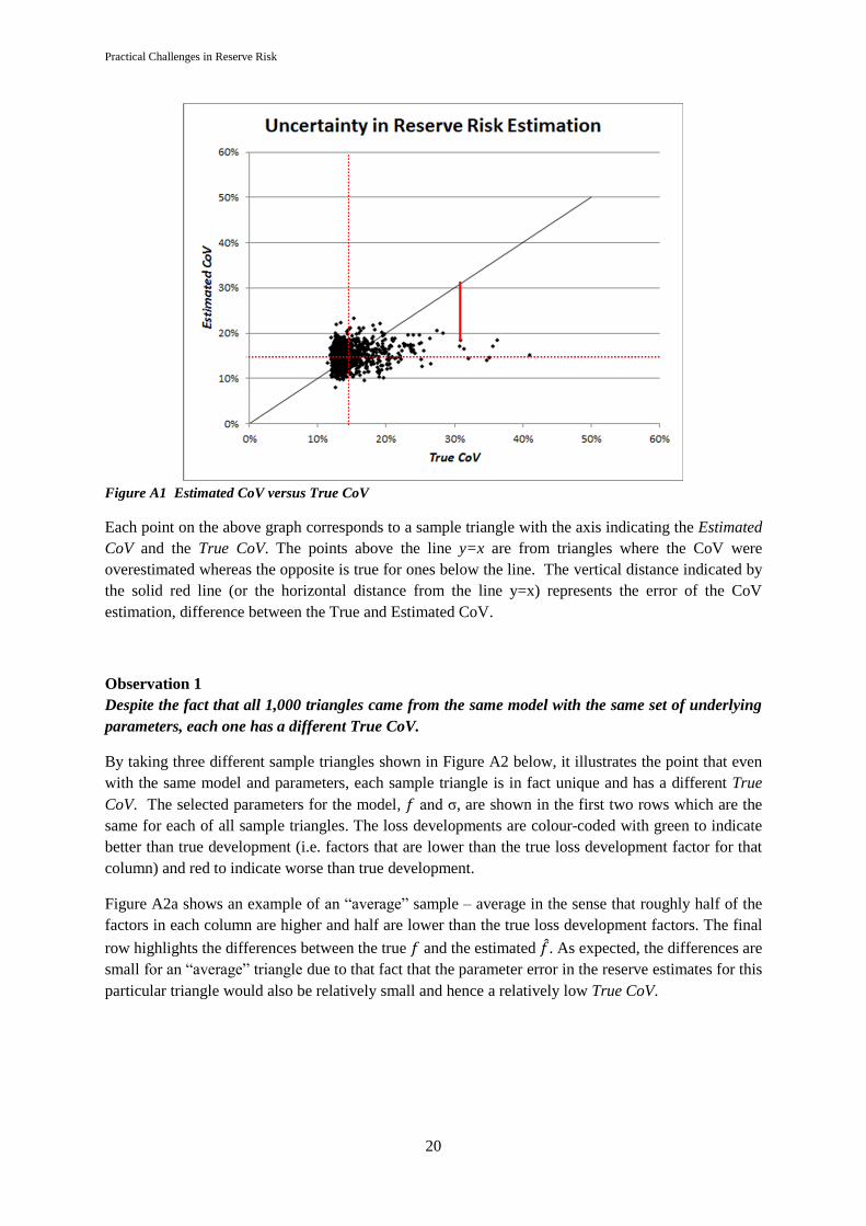
Figure A1 Estimated CoV versus True CoV
Each point on the above graph corresponds to a sample triangle with the axis indicating the Estimated
CoV and the True CoV. The points above the line y=x are from triangles where the CoV were
overestimated whereas the opposite is true for ones below the line. The vertical distance indicated by
the solid red line (or the horizontal distance from the line y=x) represents the error of the CoV
estimation, difference between the True and Estimated CoV.
Observation 1
Despite the fact that all 1,000 triangles came from the same model with the same set of underlying
parameters, each one has a different True CoV.
By taking three different sample triangles shown in Figure A2 below, it illustrates the point that even
with the same model and parameters, each sample triangle is in fact unique and has a different True
CoV. The selected parameters for the model, 𝑓 and σ, are shown in the first two rows which are the
same for each of all sample triangles. The loss developments are colour-coded with green to indicate
better than true development (i.e. factors that are lower than the true loss development factor for that
column) and red to indicate worse than true development.
Figure A2a shows an example of an “average” sample – average in the sense that roughly half of the
factors in each column are higher and half are lower than the true loss development factors. The final
row highlights the differences between the true 𝑓 and the estimated 𝑓. As expected, the differences are
small for an “average” triangle due to that fact that the parameter error in the reserve estimates for this
particular triangle would also be relatively small and hence a relatively low True CoV.

Practical Challenges in Reserve Risk
21
Figure A2a “Average” triangle
To further elaborate on this concept, Figure A2b and Figure A2c show two “extreme” sample triangles
but in opposite directions, i.e. an “extreme unfavourable” and an “extreme favourable”. By “extreme”,
it means most of the development in the triangle happens to lie on the same side from the true 𝑓’s. In
both cases, the volume-weighted average 𝑓’s provide a relatively poor estimate of the true 𝑓’s. Hence
the true parameter error in reserve estimates for these particular triangles would be relatively high and
so would the True CoV. Note that reserve risk is about mis-estimation in either direction, so regardless
of whether the triangle shows extremely favourable or unfavourable experience, both exhibit higher
parameter error relative to the “average” triangle in Figures A2a.
It should be very clear now that despite the triangles being generated from the same model with the
same set of underlying parameters, not only would each triangle has a different reserve estimate, but
would also have a different true uncertainty in the reserve estimates. Refer to Section 3.2.6 for further
discussion on the practical implications of this observation.
2/1 3/2 4/3 5/4 6/5 7/6 8/7 9/8 10/9
f 2.20 1.40 1.20 1.10 1.01 1.01 1.00 1.00 1.00
σ 300 100 100 100 50 20 5 0 0
Developmenti 1 2 3 4 5 6 7 8 9 10
1 1,000,000 2,391,911 3,506,223 4,239,223 4,566,354 4,634,674 4,701,945 4,797,599 4,797,599 4,797,599
2 1,000,000 2,107,052 3,087,878 3,678,489 4,265,311 4,205,696 4,398,225 4,374,044 4,374,044
3 1,000,000 2,341,249 3,129,773 3,700,816 4,267,585 4,285,892 4,245,529 4,340,855
4 1,000,000 2,010,549 2,840,260 3,522,843 3,803,993 3,832,101 4,037,680
5 1,000,000 1,888,299 2,468,546 2,866,506 3,545,037 4,003,298
6 1,000,000 1,750,916 2,553,273 2,965,042 3,042,827
7 1,000,000 2,411,699 3,327,589 4,077,663
8 1,000,000 2,559,981 3,713,097
9 1,000,000 1,970,140
10 1,000,000
Developmenti 2/1 3/2 4/3 5/4 6/5 7/6 8/7 9/8 10/9
1 2.39 1.47 1.21 1.08 1.01 1.01 1.02 1.00 1.00
2 2.11 1.47 1.19 1.16 0.99 1.05 0.99 1.00
3 2.34 1.34 1.18 1.15 1.00 0.99 1.02
4 2.01 1.41 1.24 1.08 1.01 1.05
5 1.89 1.31 1.16 1.24 1.13
6 1.75 1.46 1.16 1.03
7 2.41 1.38 1.23
8 2.56 1.45
9 1.97
2.16 1.41 1.20 1.12 1.03 1.03 1.01 1.00 1.00
-0.04 0.01 0.00 0.02 0.02 0.02 0.01 0.00 0.00
Year
Year
�̂�
�̂� − 𝒇

Practical Challenges in Reserve Risk
22
Figure A2b “Extreme unfavourable” triangle
Figure A2c “Extreme favourable” triangle
2/1 3/2 4/3 5/4 6/5 7/6 8/7 9/8 10/9
f 2.20 1.40 1.20 1.10 1.01 1.01 1.00 1.00 1.00
σ 300 100 100 100 50 20 5 0 0
Developmenti 2/1 3/2 4/3 5/4 6/5 7/6 8/7 9/8 10/9
1 2.36 1.45 1.24 1.05 1.04 1.02 1.00 1.00 1.00
2 2.75 1.33 1.25 1.21 0.81 1.01 1.00 1.00
3 2.51 1.45 1.19 1.13 1.02 1.00 1.00
4 2.46 1.34 1.20 1.06 1.00 1.01
5 1.90 1.40 1.26 1.14 0.97
6 2.28 1.57 1.28 1.03
7 2.31 1.51 1.11
8 2.35 1.42
9 2.05
2.33 1.43 1.22 1.10 0.96 1.01 1.00 1.00 1.00
0.13 0.03 0.02 0.00 -0.05 0.00 0.00 0.00 0.00
Year
�̂�
�̂� − 𝒇
2/1 3/2 4/3 5/4 6/5 7/6 8/7 9/8 10/9
f 2.20 1.40 1.20 1.10 1.01 1.01 1.00 1.00 1.00
σ 300 100 100 100 50 20 5 0 0
Developmenti 2/1 3/2 4/3 5/4 6/5 7/6 8/7 9/8 10/9
1 2.09 1.42 1.12 1.13 0.98 1.00 1.00 1.00 1.00
2 1.96 1.43 1.14 1.05 0.97 1.08 1.01 1.00
3 1.63 1.38 1.18 1.11 0.99 1.01 0.99
4 2.15 1.19 1.28 1.01 1.07 0.95
5 1.95 1.37 1.18 1.16 1.01
6 2.19 1.36 1.16 1.06
7 2.08 1.44 1.12
8 2.18 1.35
9 2.21
2.05 1.37 1.17 1.08 1.00 1.01 1.00 1.00 1.00
-0.15 -0.03 -0.03 -0.02 -0.01 0.00 0.00 0.00 0.00
Year
�̂�
�̂� − 𝒇

Practical Challenges in Reserve Risk
23
Observation 2
The True CoV has a wider range than the Estimated CoV.
As may be expected, “average” triangles like the one Figure A2a are typical triangles observed and the
Estimated CoV would be relatively close to the True CoV corresponding to the cluster of points around
y=x in Figure A1 whereby the Estimated CoV is closer to the True CoV. However why are there points
skewed to the right where the True CoV is much higher than the Estimated CoV?
The answer to this question will be more obvious by referring back to the “extremely unfavourable”
triangle in Figure A2b. As mentioned before, this triangle has a relatively high True CoV due to
relatively higher parameter error as indicated in the final row. Now imagine that the true 𝑓’s are
unknown as in reality without any indication of green or red, the CoV will have to be estimated based
on the triangle. Though this is an “extremely unfavourable” triangle, but in fact, it appears to be very
stable since most of the developments happen to be clustered on the same side from the true 𝑓’s (higher
in this case)! So in practice the Estimated CoV would be relativity lower than the True CoV.
What about the “extreme favourable” triangle in Figure A2c? This triangle also has a relatively high
True CoV for the same reasons above, but because most of the developments also happen to be clustered
on one side (lower in this case), the observed triangle looks relatively stable and hence would lead to a
relatively low Estimated CoV as well. It should be clear now why both “extreme unfavourable” and
“extreme favourable” triangles would lead to a significant underestimation of reserve uncertainty while
the “typical” triangles would cluster near y=x as indicated in Figure A1.
This observation clearly illustrates a limitation of the estimation process since the range of Estimated
CoV is narrower than the True CoV range indicating that in the extreme cases, the estimated reserve
uncertainty could be significantly underestimated.
Observation 3
The average Estimated CoV is approximately the same as the average True CoV across the 1,000
triangles. Moreover, majority of the time the CoV will be overestimated but in the extreme case, it
could be significantly underestimated.
It might sound concerning that triangles coming out from the same model with same set of parameters
could have a wide range of Estimated CoV and even a wider range of True CoV, but the good news is
that on average they are correct! The average True CoV across the 1,000 triangles matched closely to
the average Estimated CoV across the 1,000 triangles. The estimation process works, on average! In
other words, the difference between the true and estimated MSEP varies on different sample triangles
but on average it is close to zero1. The histogram below shows the skewness of the error distribution
of the 1,000 triangles. Note that for the majority of the time the CoVs were overestimated but in the
extreme case, it could be substantially underestimated.
1This difference can also be viewed as the parameter error in estimating MSEP since the Estimated CoV is calculated based
on data, one triangle in this case, and any estimate based on data contains parameter error.

Practical Challenges in Reserve Risk
24
Figure A3 Distribution of Error in CoV
Not only did this observation reassure that the implementation of this study was done correctly, but it
also demonstrated the remarkable fact that based on just one triangle, without knowing the true
parameters, the estimated reserve uncertainty is, in fact, correct on average2.
Observation 4
Given a triangle with an Estimated CoV, the range and distribution of the True CoV can vary
significantly.
Since the True CoV is not observable in reality, what most practitioners should be interested is the
horizontal cross-section distribution of Figure A1. In other words, given the value of Estimated CoV
what could be the range and distribution of the True CoV? This directly addresses the original question
of this study – while reserving estimates the mean and reserve risk estimates “how wrong” is the reserve,
this study examines “how wrong” is the estimation of reserve risk.
Below are two cuts of the cross-section of 1% of the width of the Estimated CoV centred at 13.5% and
at 18.5%. The thin black line indicates the average of True CoV while the red line indicates the
Estimated CoV. For the first case, Figure A4a, 75% of the time the True CoV is between 12% to 15%
and 5% of the time it is above 20%. So most of the time the Estimated CoV will be higher or within a
close range, but in the unfortunate case where the observed is an “extreme triangle” like ones in Figure
A2b and A2c, the CoV would be significantly underestimated, which leads to an underestimation on
average.
2A subtle point should be made is that the average Estimated CoV and the average True CoV will not match exactly. This is
due to the fact that, the Mack formulae in Equation 2.2.1 for the Estimated CoV is not an unbiased estimator of the True CoV.
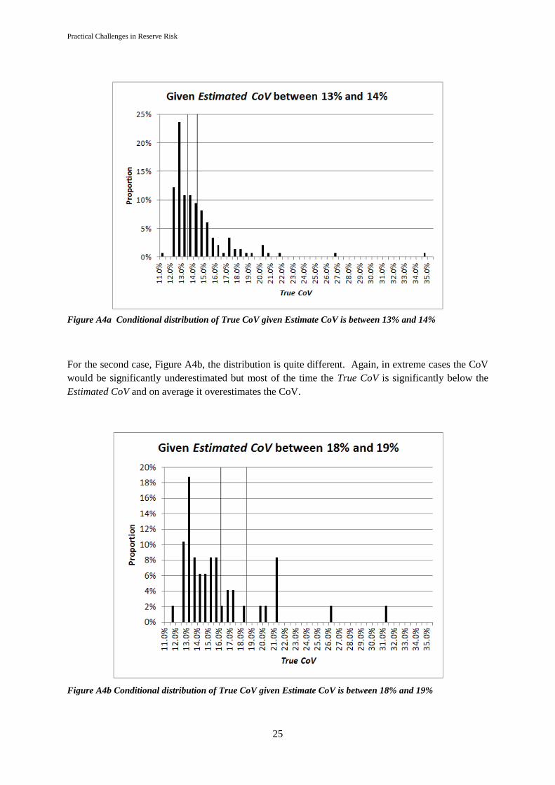
Practical Challenges in Reserve Risk
25
Figure A4a Conditional distribution of True CoV given Estimate CoV is between 13% and 14%
For the second case, Figure A4b, the distribution is quite different. Again, in extreme cases the CoV
would be significantly underestimated but most of the time the True CoV is significantly below the
Estimated CoV and on average it overestimates the CoV.
Figure A4b Conditional distribution of True CoV given Estimate CoV is between 18% and 19%
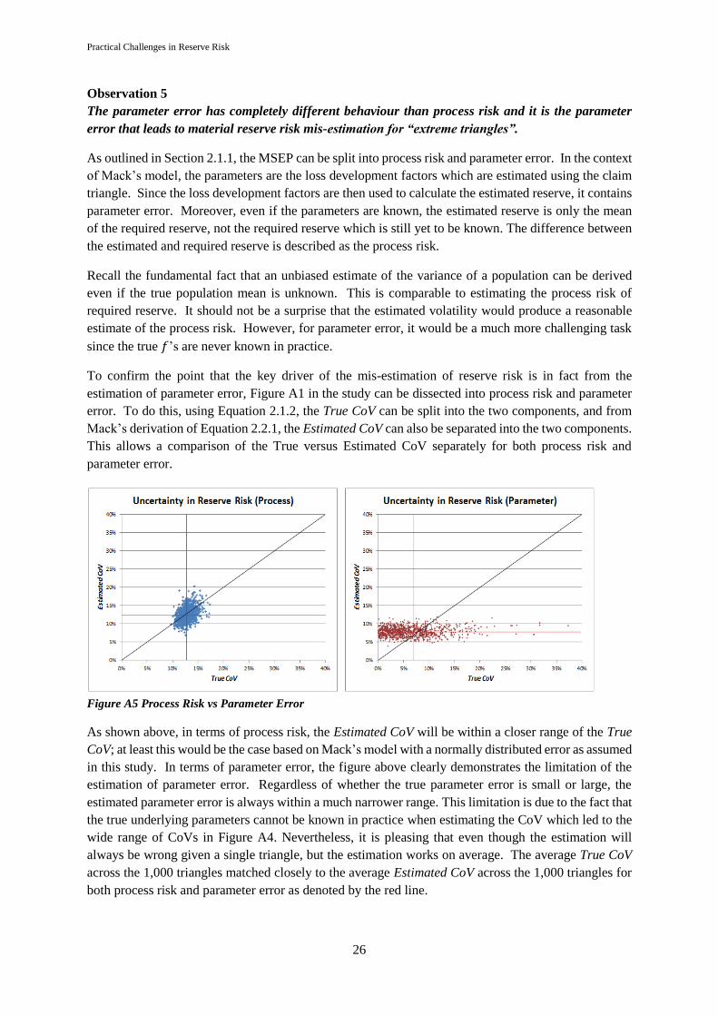
Practical Challenges in Reserve Risk
26
Observation 5
The parameter error has completely different behaviour than process risk and it is the parameter
error that leads to material reserve risk mis-estimation for “extreme triangles”.
As outlined in Section 2.1.1, the MSEP can be split into process risk and parameter error. In the context
of Mack’s model, the parameters are the loss development factors which are estimated using the claim
triangle. Since the loss development factors are then used to calculate the estimated reserve, it contains
parameter error. Moreover, even if the parameters are known, the estimated reserve is only the mean
of the required reserve, not the required reserve which is still yet to be known. The difference between
the estimated and required reserve is described as the process risk.
Recall the fundamental fact that an unbiased estimate of the variance of a population can be derived
even if the true population mean is unknown. This is comparable to estimating the process risk of
required reserve. It should not be a surprise that the estimated volatility would produce a reasonable
estimate of the process risk. However, for parameter error, it would be a much more challenging task
since the true 𝑓’s are never known in practice.
To confirm the point that the key driver of the mis-estimation of reserve risk is in fact from the
estimation of parameter error, Figure A1 in the study can be dissected into process risk and parameter
error. To do this, using Equation 2.1.2, the True CoV can be split into the two components, and from
Mack’s derivation of Equation 2.2.1, the Estimated CoV can also be separated into the two components.
This allows a comparison of the True versus Estimated CoV separately for both process risk and
parameter error.
Figure A5 Process Risk vs Parameter Error
As shown above, in terms of process risk, the Estimated CoV will be within a closer range of the True
CoV; at least this would be the case based on Mack’s model with a normally distributed error as assumed
in this study. In terms of parameter error, the figure above clearly demonstrates the limitation of the
estimation of parameter error. Regardless of whether the true parameter error is small or large, the
estimated parameter error is always within a much narrower range. This limitation is due to the fact that
the true underlying parameters cannot be known in practice when estimating the CoV which led to the
wide range of CoVs in Figure A4. Nevertheless, it is pleasing that even though the estimation will
always be wrong given a single triangle, but the estimation works on average. The average True CoV
across the 1,000 triangles matched closely to the average Estimated CoV across the 1,000 triangles for
both process risk and parameter error as denoted by the red line.

Practical Challenges in Reserve Risk
27
Observation 6
The uncertainty in the estimation of reserve risk behaves differently by accident year; both the
parameter error and process risk.
So far, the focus has been on the reserve risk for the total reserve of all accident years. It should not
be a surprise that the same graphs of Estimated CoV versus True CoV could vary significantly by
accident year. The reserve for less developed accident years are based on more loss development
factors, hence larger parameter error, and since those are the accident years where it takes more
development periods to reach ultimate, hence more process risk as well. The proportion of parameter
error and process risk could vary significantly between accident years.
To illustrate this point, Figure A6 display both the parameter error and process risk for the most recent
three accident years of the study: Year 8, 9, and 10. It is recommended to focus on the shape of the
distribution rather than the magnitude since the reserve amount, the denominator of CoV, differ by
accident years. For example, Year 8 is more developed and hence it consists of less process risk and
parameter error even though the graph might indicate otherwise due to a smaller reserve in the
denominator.
Note that as indicated by the red lines, the Estimated CoV is the very close to the True CoV for each
component and for each accident year on average across the 1,000 triangles. Again, it is evident that
the estimation process works, on average.
Conclusion
This appendix illustrated many interesting observations based on a simple question. It provided a
deeper understanding of what reserve risk is trying to quantify. From examining some sample triangles,
the concept of True CoV versus Estimate CoV becomes more apparent and the distinction between the
two sources of reserve risk becomes much more clear.
This study demonstrated the potential magnitude of uncertainty in the reserve risk estimate. Even in a
short-tail stable case assuming the model is known (i.e. no model specification error), the True CoV
could be significantly different from the Estimated CoV. It is not uncommon for some practitioners
and regulators to react strongly to relatively small changes in CoV when in truth the movement may
not be statistically significant as the estimate itself could contain large uncertainty. Such concerns
may detract from more important issues in the process.
As mentioned earlier, the objective is to draw attention to the uncertainty surrounding the estimation
of reserve risk and not to criticise one of the most common estimation methods of reserve risk in the
industry. The results highlighted the importance of validation and warn against a false sense of
accuracy especially the error in model specification could be as material, if not significantly more.
This study is an educational piece for practitioners as it provides a valuable insight in the topic of
estimation of reserve risk.
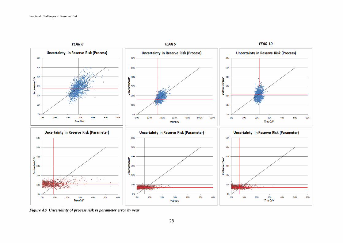
Practical Challenges in Reserve Risk
28
Figure A6 Uncertainty of process risk vs parameter error by year

Practical Challenges in Reserve Risk
29
APPENDIX B – Diversification Adjustment
As illustrated in section 3.2.4 to 3.2.6, using CoV as a risk measure is not ideal in all situations. The
CoV is the prediction error expressed as a percentage of reserve. Using CoV as a comparative measure
of reserve risk basically assumes prediction error would move by the same proportion as the reserve
moves. This appendix outlines a general approach to adjust for the non-linear relationship between
prediction error and reserve.
The rationale behind this is if the amount of business written has been doubled, with everything else
being equal, it would have doubled the number of claims resulting in a more stable triangle due to
diversification and hence the triangle would contain less process risk. Since the parameters are derived
from the triangle, it would also lead to less parameter error. This means before drawing comparison
between CoVs of two lines of business, they must be adjusted to the same volume. Here is a general
diversification adjustment approach.
Let Xi be a random variable with mean µ, standard deviation σ, and correlation coefficient between any
two Xi’s is ρ. Now, let Y be the sum of y Xi’s. The mean and variance of Y can be easily calculated:
𝐸[𝑌] = 𝑦µ and 𝑉𝑎𝑟(𝑌) = 𝑦σ2 + 𝑦(𝑦 − 1)ρσ2
So, 𝐶𝑜𝑉(𝑌) = σ√1 + ρ(𝑦 − 1) / √𝑦µ
Similar, let Z be the sum of z Xi’s, so 𝐶𝑜𝑉(𝑍) = σ√1 + ρ(𝑧 − 1) / √𝑧µ
The ratio of the two CoVs would be:
𝐶𝑜𝑉(𝑍)/ 𝐶𝑜𝑉(𝑌) = √𝑦√1 + ρ(𝑧 − 1) / √𝑧√1 + ρ(𝑦 − 1)
The above formula provides a practical and simple way to adjust for the diversification effect due to
volume for lines of business applicable for both underwriting and reserve risk. In practice, the
correlation between two incurred claims would be very low. For example, assuming 5% correlation
between any two claims (i.e. ρ = 0.05), if a line of business with a 100 claims (i.e. y = 100) has a CoV
of 10% doubled in volume (i.e. z = 200), the CoV would be 9.6%. In practice, if the number of claims
is not readily available, though not ideal, but the reserve amount could be used as a proxy for the claim
volume.
With this in mind and as concluded in Section 3.2.4, the CoV should not be used in isolation and must
be considered in conjunction with the volume. Either for the purpose of comparing CoV across different
lines of business or using CoV as a benchmark, the CoV must be adjusted with respect to the volume
accordingly.

Practical Challenges in Reserve Risk
30
APPENDIX C – “Netting Down” A Gross Aggregate Distribution
To generate a net (of reinsurance recoveries) reserve distribution, one approach is to directly model net
of reinsurance data without explicit consideration of the reinsurance program in place. While this
approach is practical to implement, it raises questions about the appropriateness. For example, any
method applied on a net triangle will not be able to distinguish if a low development is due to good
experience or due to bad experience but good reinsurance program. And, if a class had material recovery
with changing reinsurance program throughout its history, by applying bootstrapped where residuals
are resampled across different accident years will hardly give any meaningful result at all. Hence, a
more intuitive approach is to first analyse gross of reinsurance data to obtain the gross reserve
distribution before capturing the reinsurance impact. This is described as “netting down” in this
document.
Since gross reserve distribution is on an aggregated claim level, netting down is trivial for an aggregate
reinsurance program but the task becomes challenging for individual claim/occurrence based
reinsurance structure. Refer to [4] for a pragmatic netting down method, the “Conditional Ceded”
method, by incorporating individual excess of loss reinsurance programs which can then be extended
to other reinsurance programs. Below is a high level overview to briefly illustrate the framework.
Given an empirical gross distribution from say a gross bootstrap, this netting down method relies on
deriving the “ceded curve”, the expected ceded conditional on each gross amount (hence the name
“Conditional Ceded” method). This concept is easy to visualise in the following diagram and using
ultimate instead of reserve amount:
Where:
x-axis is gross ultimate loss
y-axis is gross ultimate loss but gross basis for the blue curve and ceded for the red curve
Blue curve represents gross distribution (line y=x)
Red curves represent three ceded distributions: Straight line represents quota share while the other two represent
two examples of excess of loss programs.
For the excess of loss ceded curve, it is initially flat and recoveries begins after a certain threshold of gross
amount
The average height across the ceded curve represents the mean and should tie back to ceded booked ultimate.
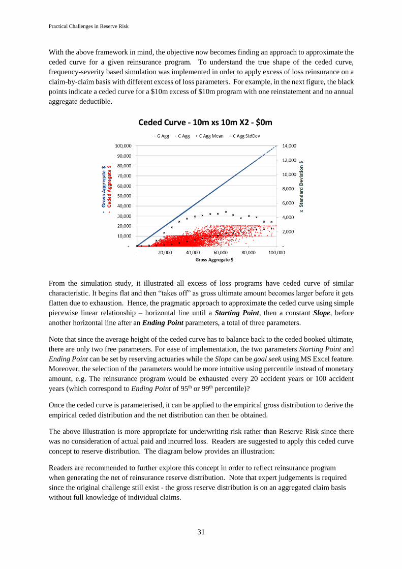
Practical Challenges in Reserve Risk
31
With the above framework in mind, the objective now becomes finding an approach to approximate the
ceded curve for a given reinsurance program. To understand the true shape of the ceded curve,
frequency-severity based simulation was implemented in order to apply excess of loss reinsurance on a
claim-by-claim basis with different excess of loss parameters. For example, in the next figure, the black
points indicate a ceded curve for a $10m excess of $10m program with one reinstatement and no annual
aggregate deductible.
From the simulation study, it illustrated all excess of loss programs have ceded curve of similar
characteristic. It begins flat and then “takes off” as gross ultimate amount becomes larger before it gets
flatten due to exhaustion. Hence, the pragmatic approach to approximate the ceded curve using simple
piecewise linear relationship – horizontal line until a Starting Point, then a constant Slope, before
another horizontal line after an Ending Point parameters, a total of three parameters.
Note that since the average height of the ceded curve has to balance back to the ceded booked ultimate,
there are only two free parameters. For ease of implementation, the two parameters Starting Point and
Ending Point can be set by reserving actuaries while the Slope can be goal seek using MS Excel feature.
Moreover, the selection of the parameters would be more intuitive using percentile instead of monetary
amount, e.g. The reinsurance program would be exhausted every 20 accident years or 100 accident
years (which correspond to Ending Point of 95th or 99th percentile)?
Once the ceded curve is parameterised, it can be applied to the empirical gross distribution to derive the
empirical ceded distribution and the net distribution can then be obtained.
The above illustration is more appropriate for underwriting risk rather than Reserve Risk since there
was no consideration of actual paid and incurred loss. Readers are suggested to apply this ceded curve
concept to reserve distribution. The diagram below provides an illustration:
Readers are recommended to further explore this concept in order to reflect reinsurance program
when generating the net of reinsurance reserve distribution. Note that expert judgements is required
since the original challenge still exist - the gross reserve distribution is on an aggregated claim basis
without full knowledge of individual claims.

Practical Challenges in Reserve Risk
32
Readers are recommended to further explore this concept in order to reflect underlying reinsurance
programs when deriving the net of reinsurance reserve distribution. Note that expert judgement is
required since the original challenge still exist - the gross reserve distribution is on an aggregated
claim basis without full knowledge of individual claims.

Practical Challenges in Reserve Risk
33
REFERENCES
[1] Alai, D. H., Merz, M., and Wuthrich, M.V. (2009). Mean square error of prediction in the Bornhutetter-
Ferguson claims reserving method. Annals of Actuarial Science 4, 7-31.
[2] Alai, D. H., Merz, M., and Wuthrich, M.V. (2010). Prediction Uncertainty in the Bornhuetter-Ferguson Claims
Reserving Method: Revisited. Annals of Actuarial Science 5, I, 7-17.
[3] Arora, A & Chan, K (2015). “We had a good year, but why has the CoV increased?” Institute and Faculty of
Actuaries. General Insurance Research Organising (GIRO) 2015 Conference Workshop D1
https://www.actuaries.org.uk/documents/d01-reserve-risk-we-had-good-year-why-has-cov-increased
[4] Chan, K & Ramyar, M (2014). “How to Net Down an Aggregate Gross Distribution?” Institute and Faculty
of Actuaries. General Insurance Research Organising (GIRO) 2014 Conference Workshop D3
http://www.actuaries.org.uk/research-and-resources/documents/d3-how-net-down-aggregate-gross-distribution-1
[5] England, P. D. & Verrall, R. J. (1999). Analytic and bootstrap estimates of prediction errors in claims
reserving. Insurance: Mathematics and Economics, 25, 281-293.
[6] England, P. D. (2001). Addendum to ‘Analytic and bootstrap estimates of prediction errors in claims
reserving’. Actuarial Research Paper No. 138, Department of Actuarial Science and Statistics, City University,
London, EC1V 0HB
[7] England, P. D. & Verrall, R. J. (2002).Stochastic Claims Reserving in General Insurance. British Actuarial
Journal, 8-3: 443-554.
[8] England, PD and Verrall, RJ (2006), Predictive distributions of outstanding claims in general insurance. Annals
of Actuarial Science 1, II, 221–270.
[9] Mack, T. (1993). Distribution-free calculation of the standard error of chain-ladder reserve estimates. ASTIN
Bulletin, 23, 213-225.
[10] Mack, T. (2006). Parameter Estimation for Bornhuetter-Ferguson. Casualty Actuarial Society Forum, Fall
2006: 141-157.
[11] Mack, T. (2008). The Prediction Error of Bornhueter-Ferguson. Casualty Actuarial Society E-Forum, Fall
2008: 222-240.
[12] Merz, M., Wüthrich, M.V., 2008. Modelling the Claims Development Result for Solvency Purposes. CAS
E-Forum, Fall 2008, 542-568.
[13] Renshaw, A. E. & Verrall, R. J. (1994). A stochastic model underlying the chain-ladder technique.
Proceedings XXV ASTIN Colloquium, Cannes.
[14] SCOLLNIK, D.P.M. (2001). Actuarial modelling with MCMC and BUGS. North American Actuarial
Journal, 5 (2), 96-125.
[15] White, S. & Margetts, S (2010) A link between the one-year and ultimate perspective on insurance risk.
Institute and Faculty of Actuaries. General Insurance Research Organising (GIRO) 2010 Conference Workshop
D3 http://www.actuaries.org.uk/system/files/documents/pdf/workshop-d03-stuart-white-simon-margetts.pdf