Practical 1 - Getting started with ArcGIS Key learning ... · Practical 1 - Getting started with...

of 18 (document version 1)

Practical 1 - Getting started with ArcGIS

Key learning outcomes:

Getting ArcGIS up and running

Setting map parameters

Adding raster data

Adding vector data

Joining data from a table

Creating a shapefile from a table

Exploring the map

(OPTIONAL: georectification)

1. Getting ArcGIS up and running

The practical element of this course will take the form of a case study of a small fictional region within the UK. A farmer local

to the village of Proudmoore has put in an application for planning permission to develop an area of land next to his farmyard

into a small theme park called “Agropolis - The Ancient Greek Farming Experience”. This will involve extensive building work

likely to disturb any archaeological material that might be hidden beneath the ground. As a caseworker in the office of the

Goldshire County Archaeologist, it is your job to determine what level of archaeological intervention should be recommended

as part of any planning conditions. You have already commissioned a geophysical survey and collated together all of the

available evidence. Now, you will use GIS to combine and analyse that evidence, to help you to reach the best possible

conclusion.

In order to complete this practical, you will need access to ArcGIS Desktop.1 You may be able to run it over your university

network or you may be able to obtain a copy for local installation: in the latter case, make sure you obtain as fully functional a

version as possible (i.e. including the ArcInfo workstation). When installing ArcGIS locally, make sure to follow the instructions

carefully (e.g. you may need to install the License Manager prior to installing the main software), and make sure you download

any relevant service packs from the ESRI website.2 If you have any problems with this, please consult with your university’s IT

services, or with your department.

Before we start working with ArcGIS, it is prudent to cover some areas of best practice:

File and directory names need to be kept simple: it is best to restrict yourself to 13 characters, to avoid using spaces, and

to only use letters, numbers and the underscore (i.e. _ ). Try to keep your directory structure simple and close to the root

of the drive, i.e. something along the lines of C:\Workspace\

1 Please note that these practicals have been tested under ArcGIS 9.1 and 9.2. Later versions of the software may contain some minor differences in wording, menus and icons. 2 See http://support.esri.com/index.cfm?fa=downloads.patchesServicePacks.gateway

http://support.esri.com/index.cfm?fa=downloads.patchesServicePacks.gateway


If running ArcGIS over a network, it is best to avoid using your network storage area to save your data. Ideally, save all of

your data to an external hard drive or other USB storage device. If you use any high resolution raster datasets, you will

need a lot of disk space.

Once you have set up a directory structure and copied over your data files, try to avoid moving them around, as the

software will easily get confused if things move unexpectedly.

Save regularly, as ArcGIS can be somewhat prone to crashes, and make sure you back up all of your data at least daily.

Use ArcCatalog if you want to delete or rename data files (see below).

If any of the buttons referred to below are not present in your version of ArcMap, go to the “View” menu, hover over

“Toolbars” and make sure that the following are both ticked: “Standard” “Tools”. Also make sure that “Status Bar” is ticked

on the “View” menu itself.

First obtain the zip file containing the data needed to complete these practicals. Extract the data files to a suitable directory in

your chosen workspace.

2. Setting map parameters

Now we are ready to get started. We shall be using primarily two pieces of software that form part of ArcGIS: ArcMap and

ArcCatalog. Start by loading up ArcMap. The software should start and normally you will be presented with a window as

follows:3

Make sure “A new empty map” is selected, then press “OK”. If this window does not

appear, it has simply been disabled by a previous user (by ticking the “Do not show

this dialog again” box), and you should just continue regardless.

You will now be presented with the main ArcMap interface, from which we will access

all of the tools and functions that we shall need to complete these three practicals.

Before we start to add data to our new map, we need to set several parameters.

3 Note that some of the screenshots included in these practicals may be slightly different from what you see on screen, depending on which version of ArcGIS you are using and where you have the toolbars placed.


Firstly, we shall save our new map. From the “File” menu, select “Save”, then save your new map to a suitable location

(ideally the same place to which you extracted the data files) using a suitable name. This new file will be an .mxd ArcMap

document. This is essentially a container document that includes the locations of any data layers and information on how they

should be displayed. Any data that you add to the map is not saved in the .mxd file, simply linked to by it.

Next, we want to set the file properties so that the saved file uses only the directory paths

relative to where you saved the map. The standard option

will remember the full paths for each data layer that you

add to the map: this becomes a problem if you decide to

move something around, or if the name of a directory or a

drive letter changes. As such, it is best to tell ArcMap only

to remember paths relative to where you just saved the

map document. This gives you a bit more flexibility in your

work methods. To do so, return to the “File” menu and

select “Document Properties” (“Map Properties” in ArcGIS

9.1). Then click on the “Data Source Options…” button in the lower right corner.


Select “Store relative path names”, then click on “OK” in both forms (In ArcGIS 9.2 and

later, you can tick the box if you wish to make this the default setting).

As we shall be using several different extensions to ArcGIS, we want to make sure that any

that we might need are available to us. These extensions contain various extra tools that

can be used to analyse our data, etc. (and would include most tools that you might download

from the internet). To do this, go to the “Tools” menu

and select “Extensions…”. Tick as many boxes as your

licences allow. Just click “OK” if you get any licence

warnings. That simply means that you will not be able

to use any tools associated with those particular

licences, which should not be a problem for the completion of these practicals. The most

important extensions in the list are the “Spatial Analyst” and “3D Analyst” extensions,

which contain the various tools used to deal with the creation and manipulation of raster

surfaces (more on which later). When you are done ticking boxes, click on “Close”.

Finally, we shall set the map projection that we wish to use for the project in hand. As we are

working with British data, we want to set the projection to the British National Grid. From the

bottom of the “View” menu, select “Data Frame Properties…”. You will see a form with a large

number of tabbed headings at the top. Click on the “Coordinate System” tab to go to that page.

In the bottom left quarter of the form, you should see

a directory list headed “Select a coordinate system”.

This contains all of the projection systems included

as standard in ArcGIS. As you will soon see, there

are a very large number of these. Open up the “Predefined” folder by clicking on

it, then “Projected Coordinate Systems”, then “National Grids”. Scroll down the

list until you find “British National Grid” and click on that one. You should see that

the projection details all appear in the upper window on the form. Click on the

“Add to Favorites” button. From now on, you will be able to select this coordinate

system from the “Favourites” folder without having to find it every single time.

Leave the form open for now.


Our study area for the case in hand is about three kilometres across east to west,

by two kilometres north to south. Therefore, the best map unit for exploring our

data would be metres. With the “Data Frame Properties” form still open, click on

the “General” tab to open up that particular form. Here we can set the preferred

map units. The units in which the map is structured are defined by the projection,

but we can change the display units, using the appropriate drop down box. Make

sure this is set to “Meters”, then click on “OK” to close the form. Make sure to

save your progress .

3. Adding raster data

Now we are finally ready to start adding some data to our map. Firstly, we shall add the DEM that provides us with information

about the background topography of our study region. We add data by clicking on the “Add Data” button on the main

toolbar. Click on the button. Before we add the data, we want to add a link to

the folder where it is stored. We do this by

clicking on the “Connect to Folder” button .

Navigate your way to the folder where you stored

the practical data in the window that pops up, click

on it so that its path appears in the box over the

folder list, then click “OK” . When we return to the

“Add Data” window, you should now be in the project folder and should be able to see all of the

various layers that we can add to the map. The icons next to each data layer show you what type of data they are constructed

from. We are currently interested in the raster layers, represented by a small grid icon . Click on the file called “dem_sp”,

then click “Add”.

The DEM should appear on your map, as a rectangular field coloured according to elevation. To the left of the map, you will

see a list of all of the layers added to the map. At the moment, this should just show the DEM layer, and it will describe to you

what the colours of the layer represent. We shall look in further detail at recolouring layers in the next

practical, but for now try setting the colour ramp used for the DEM to something else. To do so, double

click on the symbol in the layer list. A form will pop up from which you can select different colour ramps.

Choose something that you feel is appropriate for the display of elevation and click “OK”.

Next, we want to add a small satellite image of a field near to the development site to the map. Click again on the “Add Data”

button, then select the “satellite_rect.tif” layer, and click “Add”. The satellite image should appear on your map. This has


already been rectified (see Step 8 below if you need to learn how to do this). As a result, the image has been skewed slightly

and acquired an unsightly white band around the edges. We need to hide this band. To do so, double click on the layer name

in the layer list to the left of the map. This brings up

the “Layer Properties” form, which we will explore a

little more in the next practical. Make sure you are on

the “Symbology” tab. We wish to make white areas of

this layer invisible. To do this, look for the “Display

Background Value:” item. Next to this are three small

text boxes. These represent the colours red, green,

and blue. To set the background value to white, type

the number 255 into each of these boxes (the figure 2

may be hidden when you finish), as the colour white is

made up from maximum red, green, and blue on a

scale from 0 to 255 (black would be 0, 0, 0). Next to

these boxes, it will say “as” and then there is a small drop down box with which we can

set the colour we wish to display white as. In this instance, we wish to display it as “No

color”, so that it becomes invisible on the map. Click on the little arrow and make sure

that “No color” is selected. Finally, make sure that the tickbox to the left of “Display

Background Value:” is ticked. Then click on “OK” in the “Layer Properties” form. If you

look at the satellite image, you will see that the white areas become invisible.

Add the final raster layer that we need, the results of our geophysics survey of the development site. This layer is called

“geophys_rect.tif”. Just “OK” any projection warning box. Repeat the same procedure used with the satellite image to make

its white areas translucent: this time, however, you need to make the green areas translucent rather than the white. To do so,

instead of typing 255 into each box, only do so in the middle box (this being the green channel) and type 0 into the other two

boxes. This should then make the green areas of the geophysics layer invisible. Save your progress.

4. Adding vector data

Having added the raster layers to the map, we now want to add our vector layers. Fortunately, this is done in exactly the

same way. Click on the “Add Data” button again. You will see that the vector layers (which are called shapefiles) have three

different icons: one represents point data , one line data , and one polygon data . If you look at this directory using

Windows Explorer or an equivalent, you will see that each shapefile is actually made up of a number of different files with the

same name, but different extensions. Some of the raster data also uses more than one file, with the DEM actually using a

directory of its own. As a result, problems will arise if you try to rename or delete files in the conventional fashion: it is better to

use ArcCatalog for this, which we shall encounter later on.


Add the following layers to the map: “Buildings.shp” “Development.shp” “Divisions.shp” “Lakes.shp” “Rivers.shp” “Roads.shp”,

either one at a time or by holding down the Ctrl key and selecting all of them. You should see all of

these layers appear on your map and in the layer list to the left of the map (make sure you are on

the correct list by clicking on the “Display” tab at the base of the list). The order of layers in the list

is the same as the order in which they are drawn on the map, with the layer at the top being drawn

on top, and the layer at the bottom on the bottom of the stack. If you drag layers up and down using the mouse, you can

change the order in which they are drawn. Drag the layers into a sensible order, from top to bottom: “Development”

“Buildings” “Roads” “Divisions” “Lakes” “Rivers” “geophys_rect.tif” “Satellite_rect.tif” “dem_sp”. If you untick the box next to a

layer name in the list, that layer will be hidden on the map.

The “Development” layer shows the area subject to the planning

application. If you follow the ordering above, you will notice that it

obscures the area we are actually interested in. We can get around this

in one of two ways: by making the polygon hollow, or by making it

partially transparent. Double click on the layer name to open the “Layer

Properties” form for the

development layer.

Click on the “Display”

tab. Here, we can set

the transparency of this layer, by typing a percentage figure into the text box

next to the word “Transparent:”. Type in 60 (i.e. 60% transparency) and click

on “Apply”. Assuming that the form is not

hiding the layer, you will see that it is now

partly transparent on the map. However, it

has become quite hard to see, so let us

change the colour as well. Click on the “Symbology” tab in the same form. Here you will see

a box with the title “Symbol”, containing a big button coloured with the same colour as the

layer. Click on this big button and the symbol selection form will open up. On the right hand

side, find the “Fill Color” box, and click on the drop down arrow next to it. Choose a bright

red colour, then click “OK”, then “OK” again on the “Layer Properties” form. We have now

highlighted our development area in a suitable fashion.


To change the colour of the rivers and lakes to a more suitable tone, first

double click on the symbol under “Lakes” in the layer list to the left of the map.

This will again bring up the symbol selection form. On the large and long list

that fills up most of this form, you should be able to see a preset symbol style

called “Lake”. Double click on this and the lakes will be recoloured more

sensibly. Then double click on the symbol under “Rivers” in the layer list, and

select the preset “River” symbol in the list. Now experiment with changing the

colour and style of the other vector layers that you have added to the map, until

you come up with a scheme that you are satisfied with. See if you can work

out how to change the outlines of polygons, and the thickness of lines.

If you wish to remove a layer, right click on its name in the layer list and select “Remove”. Try

this with the “Roads” layer, and then add it again to the map. Save your progress. Recall

that you are only saving the arrangement of and links to your data layers. When you remove

a layer, you simply remove it from the map without deleting the source files associated with it.

This is also why you will get errors if you move around any data files associated with a map

document when you reopen it later.

5. Joining data from a table

You should now have the makings of a useful map to further your analysis of the planning application. However, we also have

some field survey data to add to the map. Click on the “Add Data” button, then open the directory called “Survey_fields”. Here

you will see a number of shapefiles named after various fields, and also a number of tables (with the icon ) which contain

the fieldwalking results associated with these fields. Add the shapefiles, but not the tables, to the map as with the previous

layers. There should be six fields: “GromsPlace.shp” “LowerBarrens.shp” “ProudmooreField.shp” “RazorHill.shp”

“SilverpinePaddock.shp” “UpperBarrens.shp”. Make sure you have added all six of these to the map.

Right click on the name of one of the fields in the layer list and select the “Open Attribute

Table” option. This shows you the table of attributes associated with each transect in the

field. You should be able to see that there are only four attributes currently associated

with each field: three of these are standard to the shapefile (“FID”, “Shape”, “ID”), and one

is a transect identity code (“TransectID”). We can use this unique code to link the

geographical objects in each layer (in this case, the fieldwalking transects) with an

external data table containing the results of our survey: the only requirement is that the

external table also contains this code. Close the attribute table that you have open.


Start with the field “GromsPlace”. Right click on the layer name, hover over

“Joins and Relates” in the options menu, then click on “Join…”. A new form

should pop up, which we can use to join the

layer to an external data table. For item 1,

“Choose the field in this layer that the join

will be based on:”, click on the drop down

menu and select the “TransectID” field. For

item 2, “Choose the table to join to this

layer…”, click on the open file icon , then

find and select the following table on your disk: “GromsPlace.csv”, then click “Add”. At

item 3, “Choose the field in the table to base the join on”, click on the drop down list and

select “Sector”. Then click on OK. If you now open up the attribute table for

“GromsPlace” again as before and scroll across to the right, you will see that an

extensive series of extra attributes have been added to this layer. Again, close the

attribute table that you have open.


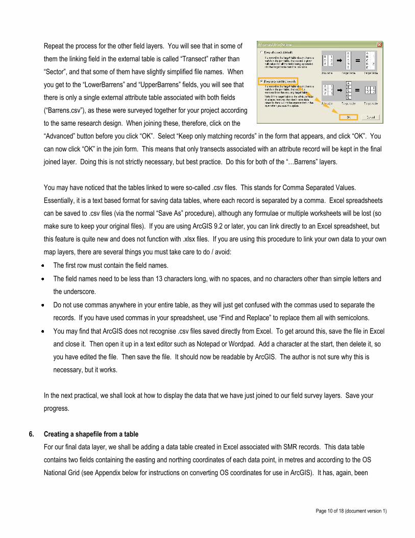
Repeat the process for the other field layers. You will see that in some of

them the linking field in the external table is called “Transect” rather than

“Sector”, and that some of them have slightly simplified file names. When

you get to the “LowerBarrens” and “UpperBarrens” fields, you will see that

there is only a single external attribute table associated with both fields

(“Barrens.csv”), as these were surveyed together for your project according

to the same research design. When joining these, therefore, click on the

“Advanced” button before you click “OK”. Select “Keep only matching records” in the form that appears, and click “OK”. You

can now click “OK” in the join form. This means that only transects associated with an attribute record will be kept in the final

joined layer. Doing this is not strictly necessary, but best practice. Do this for both of the “…Barrens” layers.

You may have noticed that the tables linked to were so-called .csv files. This stands for Comma Separated Values.

Essentially, it is a text based format for saving data tables, where each record is separated by a comma. Excel spreadsheets

can be saved to .csv files (via the normal “Save As” procedure), although any formulae or multiple worksheets will be lost (so

make sure to keep your original files). If you are using ArcGIS 9.2 or later, you can link directly to an Excel spreadsheet, but

this feature is quite new and does not function with .xlsx files. If you are using this procedure to link your own data to your own

map layers, there are several things you must take care to do / avoid:

The first row must contain the field names.

The field names need to be less than 13 characters long, with no spaces, and no characters other than simple letters and

the underscore.

Do not use commas anywhere in your entire table, as they will just get confused with the commas used to separate the

records. If you have used commas in your spreadsheet, use “Find and Replace” to replace them all with semicolons.

You may find that ArcGIS does not recognise .csv files saved directly from Excel. To get around this, save the file in Excel

and close it. Then open it up in a text editor such as Notepad or Wordpad. Add a character at the start, then delete it, so

you have edited the file. Then save the file. It should now be readable by ArcGIS. The author is not sure why this is

necessary, but it works.

In the next practical, we shall look at how to display the data that we have just joined to our field survey layers. Save your

progress.

6. Creating a shapefile from a table

For our final data layer, we shall be adding a data table created in Excel associated with SMR records. This data table

contains two fields containing the easting and northing coordinates of each data point, in metres and according to the OS

National Grid (see Appendix below for instructions on converting OS coordinates for use in ArcGIS). It has, again, been


exported as a .csv file, subject to the same restrictions as at item 5 above. However, this time the table is not associated with

any layer on the map, as it contains its own location information. This is a very useful way of importing point data to a GIS.

We shall be creating a new shapefile based upon this table. We can do this using ArcMap, but it is more robust to use

ArcCatalog. You can launch ArcCatalog from ArcMap by clicking on the ArcCatalog button . Please do so now.

ArcCatalog is essentially used to manipulate the file structures etc. of your geographic database. It is the best place to delete

or rename data layers, and also the best way to create new shapefiles. On the left there should be a list of directories, on the

right a list of the contents of whatever is currently selected on the left:

If you scroll down the list on the left, you should be able to find your main project folder for this practical, assuming you

connected to the folder as instructed earlier. Click on it, and its contents should appear on the right hand side.

The file called “SMR.csv” is what we are currently

interested in. Find it here and right click on it. You will

notice that a number of options will appear, including

the options to delete and rename. This is how you

would delete or rename your GIS data files, if you so

wished. For now, hover over “Create Feature Class”, then click on “From XY Table…”. A form

should appear. Under where it says “X Field”, select “Easting”, and under “Y Field” select

“Northing”: these are the two fields in our data table associated with the map coordinates of

each object. Ignore the “Z Field” box, as there is no elevation data associated with this layer.

Next, click on the button that says “Spatial Reference of Input Coordinates…” and the click on “Select”. We are again

choosing the projection that we wish to use, so navigate your way to “Projected Coordinate Systems\National Grids\British


National Grid.prj”, select it, and click “Add”. Then click “OK” in the spatial

reference properties form. Finally, we need to tell ArcCatalog where to save our

file. Click on the open file button

and then navigate your way to

the project directory in the usual

fashion. You should then type in a

sensible name next to “Name:”,

such as “SMR.shp”, and then click “Save”. When you return to the original

form, click on “OK” and the new shapefile layer will be built, based upon the

data in our table.

Right click in blank space in the right hand window in ArcCatalog, and select “Refresh”. You should see your

new shapefile appear. Return to ArcMap, and add this new layer to your map in the usual fashion. You should

see a series of points appear on the map. If you were to open up the attribute table for this layer (by right

clicking on its name as before), you would see that each point is associated with a number of different

attributes. Make sure this new layer is on the top of the map stack, and feel free to change the symbol if you so wish (by

double clicking on the symbol in the layer list). Save your progress. You may close ArcCatalog now if you wish.

7. Exploring the map

We now have a large amount of different data layers in our map, and we should have learned

how to add new ones, how to link data to layers, and how to create new layers from a table.

We shall now explore our data a little. If you right click on the name of a layer in the layer list,

you can select the “Zoom to Layer” option to zoom in to the extent of that layer. Experiment

with this a bit. If we click on the “Full Extent” button on the main toolbar, we will zoom out

to the full extent of the current map. The magnifying glass buttons allow you to zoom

in or out by clicking on the map, or to zoom to a selected area of the map by dragging out a

selection. The zoom in and out buttons allow us to zoom in or out by a fixed amount.

The blue arrows allow us to move back and forth between

our previously selected zoom levels. The hand button allows you to grab the map and pan it

around, by clicking and holding down the mouse button on the map, then releasing when we have it

in the desired position. Finally, there is also a drop down box for selecting a particular fixed map

scale. When moving your mouse pointer around on screen, look

down to the status bar at the bottom of the ArcMap window: at its right hand end, you will

see the current coordinates of the mouse pointer.


Feel free to experiment with these tools. If you have time and wish to learn a little about rectifying images to place them on a

map, then read on. Otherwise, save your progress, then go away and take a break. Well done, you have completed the first

practical.

8. (OPTIONAL) Georectification

Georectification is the process by which a remotely sensed raster image (e.g. an aerial photograph, a satellite image,

geophysics results, or even a scanned map) is linked in to a coordinate system so that it can be accurately located onto a

map. It is a fairly complex procedure, but this short exercise will give you a taste of how to do it using ArcGIS.

First, hide the following layers by unticking them in the layer list: “Development”

“satellite_rect.tif” “geophys_rect.tif” “LowerBarrens” “UpperBarrens”. Then add the

following layer to the map: “Satellite_image.tif”. This is the same satellite image as

before, but it has not been geographically located. When it is added to the map, you

will not be able to see it as it will be off screen, so right click on its name and select

“Zoom to Layer”. Next, go up to the “View” menu, hover over “Toolbars”, and then

select “Georeferencing”. A new toolbar should appear:

Use the drop down box next to “Layer:” on this toolbar to select the layer

“Satellite_image.tif”. We will be rectifying this image by selecting points that appear

in both our image and our base map, specifically the field boundaries recorded in the “Divisions” layer. To make this process

easier, make sure that the “Divisions” layer is above the “Satellite_image.tif” layer in the layer list, and make sure that the

“Divisions” layer is set to use a brightly coloured symbol. On the Georeferencing toolbar, look for the “Add Control Points”

button , and click on it. Now, when we click on the map for the first time, we shall select a point on our image that we can

also identify on our other layers. When we click for the second time, we are selecting this identified point on our other layers,

and creating a link between them.


Click on the satellite image at the point where the hedge near the south-western edge forms a shallow V-

shape (all of the control points used can be seen in the

image below). You will see that a cross is placed there on the map and your

cursor becomes another cross linked to the first by a line . On the layer list,

right click on the “dem_sp” layer and select “Zoom to Layer”. Use the

magnifying glass tool to zoom in on the area to which our satellite image

relates. Then click on the “Add Control Points” button again. You should

see that the pointer becomes a cross once more, still linked to the cross on

our satellite image. Click on the shallow V-shape where you can see it in the

“Divisions” layer. Right click on the name of the satellite image layer in the

layer list, and zoom to that layer. This time, add a point where the two

hedges meet near the northern edge of the image. Then zoom back to the

study area as before, and place the corresponding point on the base map.

The image should now appear stretched over its proper location, but still somewhat imperfectly placed. Add two further points

where the hedges meet in the north eastern corner and at the corner of the hedge to the east of the shallow V-shape. The

satellite image should now pretty closely match the background geographic data. Adding more points may sometimes

improve the accuracy, but this is not necessary in this case. Another alternative is to determine the locations of points in your

image on the ground (using GPS or similar) and then to enter them manually into the Link Table , but that is beyond the

scope of this short demonstration.


When you are finished, you would save your results by clicking on the “Georeferencing” menu button on the toolbar, and

selecting “Rectify…”. You would then select an appropriate location to save the new layer, alter any other parameters of the

transformation that you wish, and click on “Save”. You could then add this new rectified image to your map. However, there is

no need to do this in this case, as we already have a rectified version of this satellite image on the map. Therefore, when you

are done, simply close the “Georeferencing” toolbar (by clicking on the close icon in its top right corner), and remove the

“Satellite_image.tif” layer from the map. This georectification process is rather complex, so do not be alarmed if it does not

turn out perfectly. Further detail will be provided in a later module.


Appendix: data sources

Satellite images:

Landsat Satellite images and topographic data for the UK at http://landmap.ac.uk (requires Athens login)

Soviet images at http://www.scanex.ru/en/index.html

Spot images at http://www.spotimage.com/

University of Maryland archive of free data at http://glcf.umiacs.umd.edu/data/

NASA GeoCover has free small scale images at http://visibleearth.nasa.gov/

Google Earth may be downloaded from http://earth.google.com/

Digital maps:

Digimap can be a bit hard to navigate, but provides Ordnance Survey maps for UK (including historical) via Edina at

http://edina.ac.uk/digimap/ (site requires registration and you must be careful to cite copyright correctly on any finished

maps)

The USGS provides Digital Elevation Models etc. for the whole world at http://seamless.usgs.gov/

Soviet maps of Europe are available at http://maps.poehali.org/en/ or http://topomaps.eu or http://sovietmaps.com (note

that these may need significant processing to be usable)

An excellent list of sources of free or low cost geographical data is provided at

http://wiki.osgeo.org/wiki/Public_Geodata_for_the_UK (mostly for the UK, but it also includes some international sources)

http://landmap.ac.uk/

http://www.scanex.ru/en/index.html

http://www.spotimage.com/

http://glcf.umiacs.umd.edu/data/

http://visibleearth.nasa.gov/

http://earth.google.com/

http://edina.ac.uk/digimap/

http://seamless.usgs.gov/

http://maps.poehali.org/en/

http://topomaps.eu/

http://sovietmaps.com/

http://wiki.osgeo.org/wiki/Public_Geodata_for_the_UK


Appendix - Ordnance Survey coordinate conversion

OS grid references usually take the following form: SK123456 or HZ12345678, etc., depending on their precision. Here, the letters

give the location of the large 100km grid square and the numbers give the easting and northing. To enter these grid references into

a GIS, we need to split out the easting and northing into separate attributes and convert the letter portion into numbers, using the

system shown in the diagram and conversion table on the next page. We also usually need to add some zeroes to the end of each

number to make sure that the grid references are to the nearest metre.

Thus, the grid reference SK123456 would have an easting of 412300 and a northing of 345600; the 4... and 3... are read off the

diagram and the rest of the grid reference split in the middle. We have to add two zeroes to each number as this was a six figure

grid reference which is precise to the nearest 100 metres (essentially it refers to a 100m x 100m square on the ground). As another

example, HZ12345678 would have an easting of 412340 and a northing of 1056780, with the 4... and the 10... read off the diagram;

here we add one zero to each number as an eight figure grid reference is precise to the nearest 10 metres. We would not have to

add any zeroes to a ten digit grid reference, as it is already precise to one metre. We would need to add more zeroes to two and

four figure grid references, but these are very imprecise and so would be better represented as grid squares in any event.

We usually do this conversion using spreadsheet software (such as Excel) prior to entering the data into the GIS. First we would

create three fields that split the grid reference into the letter, easting and northing portions (either manually or by creating a macro).

Then we convert those eastings and northings into full coordinates by multiplying by 10 (for an eight figure grid reference) or 100

(for a six figure) and then adding on the conversion figure, e.g. 400000 to the easting and 300000 to the northing for the SK square.

The formula would looks something like this:

=(A1*10)+400000

where A1 is the cell holding the unconverted easting value.


OS conversion table:

Grid square: Easting value: Northing value: Easting metres: Northing metres:

HP 4 12 400000 1200000

HT 3 11 300000 1100000

HU 4 11 400000 1100000

HW 1 10 100000 1000000

HX 2 10 200000 1000000

HY 3 10 300000 1000000

HZ 4 10 400000 1000000

NA 0 9 0 900000

NB 1 9 100000 900000

NC 2 9 200000 900000

ND 3 9 300000 900000

NF 0 8 0 800000

NG 1 8 100000 800000

NH 2 8 200000 800000

NJ 3 8 300000 800000

NK 4 8 400000 800000

NL 0 7 0 700000

NM 1 7 100000 700000

NN 2 7 200000 700000

NO 3 7 300000 700000

NR 1 6 100000 600000

NS 2 6 200000 600000

NT 3 6 300000 600000

NU 4 6 400000 600000

NW 1 5 100000 500000

NX 2 5 200000 500000

NY 3 5 300000 500000

NZ 4 5 400000 500000

OV 5 5 500000 500000

SC 2 4 200000 400000

SD 3 4 300000 400000

SE 4 4 400000 400000

SH 2 3 200000 300000

SJ 3 3 300000 300000

SK 4 3 400000 300000

SM 1 2 100000 200000

SN 2 2 200000 200000

SO 3 2 300000 200000

SP 4 2 400000 200000

SR 1 1 100000 100000

SS 2 1 200000 100000

ST 3 1 300000 100000

SU 4 1 400000 100000

SV 0 0 0 0

SW 1 0 100000 0

SX 2 0 200000 0

SY 3 0 300000 0

SZ 4 0 400000 0

TA 5 4 500000 400000

TF 5 3 500000 300000

TG 6 3 600000 300000

TL 5 2 500000 200000

TM 6 2 600000 200000

TQ 5 1 500000 100000

TR 6 1 600000 100000

TV 5 0 500000 0

Practical 1 - Getting started with ArcGIS Key learning ... · Practical 1 - Getting started with...

Documents

Transcript of Practical 1 - Getting started with ArcGIS Key learning ... · Practical 1 - Getting started with...