Pr Hhrabs Outen, - Virginia Tech
118
THE APPLICATION OF OVERALL EQUIPMENT EFFECTIVENESS (OEE) AS A MEASURE FOR IMPROVING PRODUCTIVITY AND EFFICIENCY IN A TYPICAL FACTORY ENVIRONMENT by Chyi-Bao Yang Project and report submitted to the Faculty of Virginia Polytechnic Institute and State University in partial fulfillment of the requirements for the degree of MASTER OF SCIENCE in Systems Engineering APPROVED: Sa 8S BaD) Professor Benjamin S. Blanchard, Chairman Pr Hhrabs Outen, DY) Roderick J. Reasor Dr. Dinesh Verma July 1995 Blacksburg, Virginia Key words: Maintenance, Effectiveness, Productivity, OEE, TPM
Transcript of Pr Hhrabs Outen, - Virginia Tech
THE APPLICATION OF OVERALL EQUIPMENT EFFECTIVENESS
(OEE) AS A MEASURE FOR IMPROVING PRODUCTIVITY AND
EFFICIENCY IN A TYPICAL FACTORY ENVIRONMENT
by
Chyi-Bao Yang
Project and report submitted to the Faculty of
Virginia Polytechnic Institute and State University
in partial fulfillment of the requirements for the degree of
MASTER OF SCIENCE
in
Systems Engineering
APPROVED:
Sa 8S BaD) Professor Benjamin S. Blanchard, Chairman
Pr Hhrabs Outen,
DY) Roderick J. Reasor Dr. Dinesh Verma
July 1995
Blacksburg, Virginia
Key words: Maintenance, Effectiveness, Productivity, OEE, TPM

one
THE APPLICATION OF OVERALL EQUIPMENT EFFECTIVENESS
(OEE) AS A MEASURE FOR IMPROVING PRODUCTIVITY AND
EFFICIENCY IN A TYPICAL FACTORY ENVIRONMENT
by
Chyi-Bao Yang
Committee Chairman: Benjamin S. Blanchard
Systems Engineering
(ABSTRACT)
Many systems in use today do not fulfill their expectations when operating, and are in
a non-operating state much of the time due to maintenance. The accomplishment of
maintenance often turns out to be costly and may significantly influence performance and the
competitive position of a factory. In response to maintenance problems in the industrial
environment, “Total Productive Maintenance (TPM)” is rapidly becoming the reliable,
efficient, and cost-effective approach to maintaining the system to be operated at the full
capacity with high productivity and low production cost.
“Overall Equipment Effectiveness (OEE)” has been developed to measure the
effectiveness of a given maintenance approach. It involves all of the operation and
maintenance parameters required to measure the overall operating condition of the factory and
its equipment. Measuring in terms of the OEFE assists in identifying the production losses
experienced in a factory, and aids in planning possible countermeasures to eliminate those
losses.
The concept of TPM and the steps involved in TPM implementation is introduced. A
specific measure of TPM effectiveness, OEE, is defined, employed, and the results are
analyzed. A computerized OEE model is developed to facilitate the measurement and
evaluation process. The countermeasures necessary to eliminate the losses defined in TPM are
also discussed. Application of OEE measurement and evaluation is illustrated through a case
study assuming a hypothetical factory environment. A cost-effectiveness analysis in terms of
the total product cost and the resultant OEE value is also illustrated through the case study.
The application of these methods for continuous factory improvement is the objective.

ACKNOWLEDGMENTS
First, I wish to express my sincere gratitude to my chairman Professor Benjamin S. Blanchard
for his excellent guidance, invaluable advice, and continuous support during my graduate
studies.
I would like to extend my appreciation to Dr. Dinesh Verma for his encouragement and
continuing support and instruction. Also, I would like to extend my gratefulness to Dr.
Roderick J. Reasor for his contributions to my education and serving on my committee.
Finally, I am grateful to Ms. Judy Snoke for reviewing my project for grammatical correctness
and suggestions for improving the project's understandability.
Special thanks is given to Dr. Szu-Wei Yu (Chung-Cheng Institute of Technology, Taiwan,
R.O.C.) for his ongoing support and encouragement throughout this effort.
Additionally, I would like to thanks Ms. Loretta Tickle for her encouragement and assistance
with all paperwork. Also, I give my deepest thanks to my family and friends for their unending
patience and understanding on the road to completion.
1V
TABLE OF CONTENTS
ABSTRACT 000 cece ccccc ccs neeeecececcessssseeesseseeseeeseenecseeettesaaaneesss ii
ACKNOWLEDGMENTS ........0.... 000i eee ccccececeeceeeseseeaauaaaaeeeens iv
TABLE OF CONTENTS 000000000000 ccccccccccccceccecceeceeeeseceeeeesssneneeseseeeees Vv
LIST OF FIGURES 20.0000 c cc ccceeccccecceseeeeeeeseesessanseeeeeeeees vil
LIST OF TABLES ooo00o0ooooo ccc ccccccccccccceeceeeeeeeecceeeeeeeeeeeeesaaaeaseeneneeeeeed Vill
CHAPTER 1. INTRODUCTION 0000000... ccceneeeeeeeeees |
LL. Problem Statement .......00..cccccccccc cece cecseeccccsccceesceueeseceesesuuueecssessesannesees I
1.2. Maintenance Overview ......cccccccccccccecccces tet teteeee eee eceeeeceeecesseuaassaaaae ences 3
1.2.1. Corrective Maintenance 2.0.0.0... .0cccccccceeeeeececeee ee eeteeeseeseeeeesseeeeeeeanees 4
1.2.2. Preventive and Predictive Maintenance .................0ecseeeeeceeeee eee ecto ens 6
1.2.3. Maintenance Prevention .............cccccceeseeeeeececcececeeeeecessessueseeseeseseees 10
L.3. Eeffectiveness FQCHOIS ......ccccccccece cece e eee e cece cece eee nent et Et Eed 1]
L.4. Project ODjECHVES .ooeececcccccccccec cece eee e eee EEE 14
CHAPTER 2. TPM IMPLEMENTATION .............00000.... eee 18
2.1. Introduction to TPM oocccccccccc ccc cccccccc ccc eeccceces ee eeccceeseesseeeuuaeesseetaaeeeeeeenas 18
2.2. Characteristics of TPM .oc.c.cccccccccccc cece cece cent eee e een cece eee bene beet bette 22
2.2.1. Autonomous Maintenance ............ccccccceceecceeeeeceeeueeeeceueeeeseeetennees 22
2.2.2. Small Group Activities 000.0... .0cccccccccceeeececcceseeeseceeeeeeeeeeeteeesseeeeneees 26
2.3. Steps of TPM Development .........0cccccccvvcceececeecsccesecccceeceesseseesaseaeeneeeeeeees 29

CHAPTER 3. MEASURING TPM EFFECTIVENESS ...000000
3.1. TPM Effectiveness Medsures .occcccccccccccccccccc cece cece eee e ee eebbceeeeeeeeentaas
3.2. Overall Equipment Effectiveness ........ccccccceceevevvveveesecseccceeeesseenesaananenseees
3.3. Computerized OEE Model oo... . ccc ccccccececccc cece ec cceetnns en eeeeeeeeseetesennnnisaees
3.4. Countermeasures to Eliminate Equipment [email protected] cee ennneeeees
CHAPTER 4. CASE STUDY 0000000. c ccc cccce tees et eeeesessaeeeees
4.1. Hypothetical Factory ENVirOnment ....00ccccccccc cece cece vv cce esac cces cet neeeeeennneeees
4.2. Operational and Maintenance Records ......cccccccccccccccccec cece eee e ett nnteneeeeeeees
4.3. Effectiveness Evaluation and AnlySis ..........cc0cccccceeeeeeecccccccccceeee eee e estes
4.3.1. OEE Calculation 2.0.00... ccccecceceee nee ee cents neceee ee eeeeaeeeeeeaten ens
4.3.2. OEE Analysis and Countermeasures ...............0.00:cceececeeeeeeeeeneeeenens
4.3.3. Total Cost Analysis 2.0.0.0... ccccccc cece cece ec ence eee eeeeeeeeeneeeee seen eaenes
4.3.4. Cost-Effectiveness Analysis ..............cccccceeececneeeeeceeeeeteeeeeaeueeeeeens
CHAPTER 5. SUMMARY AND FUTURE RESEARCH ...................
DL. SUMMA Y oo ccc anne EERE EEE E EEE EEEEEEE EEE EEEE EEE EEE EEE EEE EE EEE EY
D2. Future RESCQrch occ... ccc ccc cece cece cece e cece eee e eset ee eee ene eeteeeseeaaaaenes
REFERENCES 00000... c cece cece cette eeeeeeeee sta seeeeeeeeeasananseeeeees
BIBLIOGRAPHY 000000000 ccc c cc ccccteeeceee ces eas ee eeeeseeeessaneeeeeeeeenaas
APPENDIX A. PROGRAM CODES AND OUTPUT ...0
Figure 1.1
Figure 1.2
Figure 1.3
Figure 1.4
Figure 1.5
Figure 2.1
Figure 2.2
Figure 2.3
Figure 3.1
Figure 3.2
Figure 3.3
Figure 3.4
Figure 3.5
Figure 4.1
Figure 4.2
Figure 4.3
Figure A.1
Figure A.2
LIST OF FIGURES
Corrective Maintenance Cycle .............ccccceceeeecececeeeeeeneeeneeeeeeneeeenes
Cost-versus-Delay Cufe ............ccccececeeeeneeeeeeeeeneeeeceeeseeesensneeseseenes
The Relationship between the Cost of Preventive and Breakdown
Maintenance 2.0.00... 0. cece cece ccc cec eee e een e eee ee ee en sence eeeeaeeeeeen tense eaeenenees
Elements of System Cost Effectiveness ..............ccccscceceeeceeeeecueeeeeneees
Production Process FIOW ............cccccccccccecccccccecccceseececeeeeeecnccecuuuenees
Relationship between TPM, Productive Maintenance, and Preventive
Maintenance ...........cccccec eee eee c ee ece cece ee eeeeeeen seen ec eseeseeteseneneeeeeeetetaes
TPM OVErVview 20.0.0... cece cece ec ncneeee rene eneeeeneeeneneeeeeeeeneneneaeaeeeeseeeeeees
System Development Process ..............cccccececeeeeeeeceeeeeeeeeneaeeeeneeeenees
Example of OEE Calculation 2.0.0.0... cceccccceeceecece ee eeeeeeeeeeneenees
Computerized OEE Model Flow Chart ........ 0... ccce ccc ceccceecneeceeeneerees
Improving Setup and Adjustment .............. ccc ccceeeec nee eceeeneeeeaeeeeeeeeeens
Improving Idling and Minor Stoppages ...............cseceecneececeeneeeeeeeeeees
Improving Quality ........ ccc cece cece cnet ence e eee een en ee ee een ee nea en ee ens
Impacts of Availability on OBES ..............c cece ccc ecnec cence eteee tense eeeeeenees
Impacts of Performance rate on OEEs ......... 0... cec ees ee cece ec eee eeeeneen eee ens
Cost Breakdown Structure 10.2.0... .cccceceeeeneeeneeceeeueeceeeaeeeaeeneeeuseneees
Input Screen of Computerized OEE Model ..............ccc cee eeeeeeseeeecn teens
Output of Computerized OEE Model ............ 0. ce ccc ec cccec ec eeneeeeen seen
15
16
20
23
31
37
4]
44
45
48
65
68
74
108
109
vil
LIST OF TABLES
Table 2.1 Seven Steps for Developing Autonomous Maintenance ...................066 27
Table 2.2 Twelve Keypoints of Autonomous Maintenance ............:::ccccceeeeeee 28
Table 2.3. The Twelve Steps of TPM Development ...............:cccceeeteeetseeesteeees 32
Table 3.1 Improvement Target for the Six Big Losses ...........0.:::ccseeeesseeeestsees 42
Table 3.2 — Strategies for Increasing Speed .............0cccccecsceccseseeeeesestaeeeceenaaees 46
Table 4.1 System Success Data .........0ccccccccccccceseseceeessseeeeessseeeeeeeseeeeesssaeeens 52
Table 4.2 System Maintenance Data ...........0cccccccceceesssececseeeeeterseeetsseeeensseeensas 52
Table 4.3. Maintenance Records and their Uses ..........00cccccccccsssceeeeeesessseeeeeseees 54
Table 4.4 Summary of Working Time .............cccceeecscceeeeeeessteeeeeneeeeetseeeeenaees 56
Table 4.5 Cycle Time Records ..........cccccceccsscceeneeeeeeeeceeeeeceeeeneeecnseeenteeensaeens 56
Table 4.6 Quality of Defect Records .........cccccccccesccccccsscecesensaeeeeeetseeeeenssnteees 56
Table 4.7 Summary of Downtime Records .........0.::cccccececseeeeetseeeeseeeeeseseeeesees 57
Table 4.8 = Maintenance Action Records ..........cccccccceeesscceeseeeeteseeesseeesseeeesseeens 37
Table 4.9 — Results of OEE Calculation .........0.cccccccecscecesseeesteeeeseeestseeeneees 59
Table 4.10 Results of OEE Analysis for Performance Rate ............:::cccccseesseeeees 67
Table 4.11 Results of OEE Analysis for Performance Rate .............::ccccscscceseeee 69
Table 4.12 Costs of Material Inventory Spare/Repair Parts .........00.....ccceececeeeeees 77
Table 4.13 Maintenance Costs .........0ccccccceccccssceceseeeeeeseecesseceesteteeestieesenseesents 77
Table 4.14 Total Product Cost Breakdown ...........::ccccccccesseessceeeeteeeeeeteteeeesseeens 78
Vill

CHAPTER 1
INTRODUCTION
In today’s competitive environment, manufacturing systems, in particular, are
becoming increasingly sophisticated, and their performance and effectiveness are often
inadequate to meet customer needs. Many of the systems in use are in a non-operating state
much of the time due to maintenance. Additionally, the accomplishment of maintenance often
turns out to be quite costly [Blanchard, 1994]. In order to survive in the competitive
environment and maintain the systems at full capacity, system maintenance must receive the
same attention as system performance when companies require smooth functioning, reliable,
efficient and cost-effective maintenance programs.
1.1 Problem Statement
Many systems in use today are neither performing as intended, nor cost-effective in
terms of their operation and support. Manufacturing systems often operate at less than full
capacity with low productivity and high production cost. To remain competitive in today’s
global markets, a manufacturing company needs a cost-effective system designed for peak
operation of its production machinery. Maintenance includes all actions necessary for
retaining a system in, or returning it to, its desired operating condition and serves as a major
contributor to the performance and profitability of the system [Blanchard and Verma, 1995].
From the cost standpoint, one study has revealed that from 15% to 40% of the total cost of a
product can be attributed to maintenance-related activities in the factory [Mobley, 1990].
With regard to the issue of cost due to maintenance-related activities, experience has
indicated that a large portion of product cost is caused by these high maintenance costs which
refer to the direct maintenance labor and material costs in the factories that produce the
product. This, in turn, significantly impacts sales in a highly competitive marketplace. In other
words, high maintenance costs in the factory are causing a reduction in sales and a loss of
revenue. In addition, recent surveys have shown that one third of all maintenance
expenditures is wasted because of unnecessary or improper maintenance program
implementation [Mobley, 1990]. The traditional approach to plant maintenance does not
support timely, innovative, profitable solutions to the waste, inefficiency, and cost problems
associated with previous deficiencies. As systems become more complex, it is essential that an
effective and profitable maintenance approach be implemented throughout the entire life of
the system. Consequently, a nontraditional approach to plant maintenance, which integrates
design, engineering, production, and maintenance, reduces maintenance downtime and life-
cycle cost, and applies maintenance technologies to improve equipment effectiveness, must be
implemented.
Generally, a measure of effectiveness is used to describe how well the outputs achieve
the desired goals. In practice, effectiveness is concerned with the definition, control, and
measurement of system performance [Blanchard, 1969]. In order to understand the outcomes
of a specific implementation approach and to integrate this approach more effectively
throughout the company or plant, the current problems, the potential for their solution, and
the benefits to be gained must be clarified through the analysis and measurement of
effectiveness. This approach can isolate the problems and enhance the system’s potential for
improvement. Lack of a concept of analysis and the measurement of effectiveness may lead to
redundant effort and misguided solutions. Such analysis and the measurement of effectiveness
helps to pinpoint areas which are experiencing problems, and helps to identify where those
problems are in the system. Finally, such an effort can help plan countermeasure prevention
and improve in the implementation of maintenance approach.
An “overall equipment effectiveness (OEE) model, defined in the effectiveness
measurement of “Total Productive Maintenance (TPM)” which is a new integrated life-cycle
maintenance approach, has been developed to measure the effectiveness of a given
maintenance approach [Nakajima, 1988]. OEE is the best way to measure the effectiveness of
maintenance because it considers all of the operational and maintenance parameters pertaining
to the overall operating conditions of a manufacturing system. OEE represents the product of
availability, performance efficiency, and quality rate. The causes of equipment losses can be
identified from these three parameters and the possible countermeasures for prevention can be
planned by analyzing each. In practice, experience indicates that OEE averages 45% at
companies where TPM doesn’t exist [Kotze, 1993]. Many factories are generally found to
have OEE ratings only between 40% and 60% before TPM implementation [Nakajima, 1989].
It is also sad to say that the OEE in most US companies barely break 50% [Wireman, 1994].
These poor OEE values reveal that manufacturing systems are being operated at only one-half
of their potential effectiveness, and that traditional equipment maintenance approaches are
ineffective. Referring to Nakajima [Nakajima, 1988], an OEE of 85% is considered as being
the “benchmark” for world class operations. Thus, there is so much room for improvement in
the typical equipment maintenance management program.
As a result, there is a need for current manufacturing systems to implement an
aggressive nontraditional approach to plant maintenance to increase the OEE values and
reduce manufacturing costs. It is the objective of this project to introduce the concept of TPM
and the steps involved in TPM implementation, and to present how to measure OEE values in
order to identify production losses and how to analyze an OEE value in order to plan
countermeasures to eliminate all production losses.
1.2 Maintenance Overview
With continuous industrial change and increasing competitiveness in the global
market, the concepts and practices of traditional maintenance must be updated. The overall
objective of every maintenance program should be to make the greatest possible contribution
to the long-term profitability of the company. Therefore, an effective maintenance
management program capable of maximizing the availability of plant facilities in operating

condition, permitting maximum performance, and extending the service life of plant and
equipment must be implemented.
TPM is rapidly becoming the approach of choice in this area. It constitutes the design
and development of equipment for reliability and maintainability with the objectives of: (1)
minimizing maintenance downtime; (2) reducing the requirement for support resources; (3)
improving productivity; and (4) reducing life-cycle cost [Nakajima, 1988]. According to the
observations of Dyer [Koelsch, 1993], compared to companies that still practice traditional
maintenance approach, companies that implement TPM are seeing 50% reductions in
breakdown labor rates, 70% reductions in lost production, 50% ~ 90% reductions in setup,
25% ~ 40% increases in capacity, 50% increases in labor productivity, and 60% reductions in
cost per maintenance unit. Therefore, TPM is an improved maintenance approach over the
more traditional maintenance approaches, which refer to corrective, preventive, and predictive
maintenance and maintenance prevention. TPM enhances the state of maintenance, improves
product quality, and increase productivity. It also results in reduced waste and reduced
manufacturing costs.
1.2.1 Corrective Maintenance
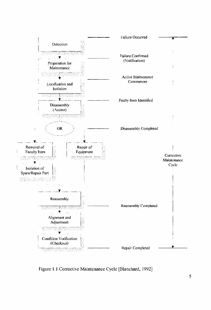
Corrective (or emergency) maintenance is merely reactive repair work that waits for
machine or equipment failure before any maintenance action is taken. Corrective maintenance
includes all unscheduled maintenance actions performed, as a result of system failure, to
recover the system to a specified operational status. Figure 1.1 illustrates a corrective
maintenance cycle which performs a series of steps to repair and restore the system to full
operating condition. This series of steps includes failure identification and verification,
localization and fault isolation, disassembly to gain access to the faulty item, item removal and
replacement with a spare or repair in place, reassembly, checkout, and condition verification
[Blanchard, 1992].
: Detection
| _t y _
Maintenance
Localization and
Isolation
Disassembly | (Access)
~ a
——_{ OR \
_
| re
|
4
[ Removal of |
| Faculty Item | |
| Isolation of
| Spare/Repair Part
y | | Reassembly
yp .
| Alignment and
Adjustment
A |
| Condition Verification
| Preparation for | -
|
|
|
|
So
Fe .
Repair of Equipment ,
| (Checkout)
Failure Occurred
—— ——
| Failure Confirmed |
(Notification) |
Active Maintenance
Commences
Faulty Item Identified
Disassembly Completed
Corrective
Maintenance
Cycle | |
| Reassembly Completed |
|
Repair Completed —_—_1___
Figure 1.1 Corrective Maintenance Cycle [Blanchard, 1992]

1.2.2 Preventive and Predictive Maintenance
Preventive maintenance includes all scheduled maintenance actions performed to
retain a system in a specific operational status. It includes: (1) those periodic inspections to
detect conditions that might cause breakdowns, production stoppages, or detrimental loss of
function; (2) maintenance to eliminate, control, or reverse such condition in their early stages;
and (3) regular maintenance activities such as lubrication, cleaning of the line, and changing of
filters, planned to prevent sudden failure of equipment and to help ensure equipment is
operating in a satisfactory manner. In other words, preventive maintenance is a periodic
maintenance to inspect equipment condition and treat equipment abnormalities before
abnormalities cause defects or losses [Nakajima, 1989].
According to Niebel [Niebel, 1994], the principle objectives of preventive maintenance
include:
1. Minimizing the number of breakdowns on critical equipment
Reducing the loss of production that occurs when equipment failure takes place
Increasing the productive life of all capital equipment
- Ye
NS
Acquiring meaningful data relative to the history of all capital equipment so that
sound repair, overhaul, or replacement decision can maximize the return on capital
investment
5. Permitting better planning and scheduling of required maintenance work
6. Promoting improved work force health and safety.
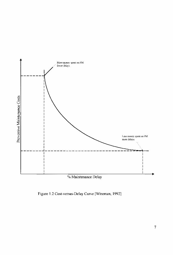
From the cost perspective, maintenance costs are a major part of the total operating
cost of all manufacturing and production plants. The overall objective of maintenance is to
maximize the production performance at a minimum cost. A typical cost-versus-delay curve is
illustrated in Figure 1.2 [Wireman, 1992]. In order to reduce the preventive maintenance
costs, preventive maintenance is only performed when actually necessary to avoid the cost of
Preventive Maintenance
Costs
More money spent on PM
/ fewer delays
a
Less money spent on PM
more delays
“% Maintenance Delay
Figure 1.2 Cost-versus-Delay Curve [Wireman, 1992]
Vv

the lost of production time and the wasted man hours and materials. Too much preventive
maintenance can cause much downtime, the possibility of inducing damage to the related
components, and can be very costly. The point of more delay in Figure 1.2 is suggested to
reduce the money spent on preventive maintenance.
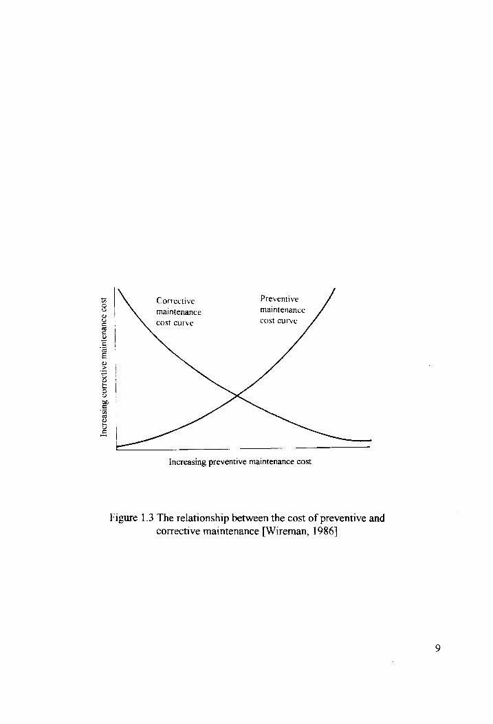
There will always be a trade-off between corrective and preventive maintenance. The
relationship between the cost of preventive and corrective maintenance is presented in Figure
1.3. The costs of preventive maintenance must be weighed against the costs of breakdown
[Wireman, 1986]. For some equipment, it is more economical to only perform maintenance
when the equipment breaks down, rather than investing the manpower and materials to
perform preventive maintenance. If the cost of preventive maintenance is greater or equal to
the cost incurred by a breakdown, then preventive maintenance would be a waste of money
and should not be executed.
The maintenance approach known as predictive maintenance, or condition-based
maintenance, is attracting attention as a highly reliable replacement for conventional periodic
preventive maintenance. Predictive maintenance refers to a condition-monitoring preventive
maintenance program where direct monitoring methods are used to determine the exact
equipment condition, for predicting possible degradation, and for pinpointing the areas where
maintenance is needed before capacity reductions or losses occur [Blanchard and Verma,
1995]. Predictive monitoring techniques include: vibration analysis; ultrasonic analysis;
thermography; tribology; process monitoring; visual inspection; and other nondestructive
analysis techniques [Mobley, 1990]. Most comprehensive predictive maintenance will use
vibration analysis as the primary tool. However, a total plant predictive maintenance program
must include several techniques depending on the equipment types, their impact on
production and plant operation, and the company’s goals. The objective is to predict when
failures will occur and to take preventive measures accordingly.
Increasing corrective maintenance
cost
Corrective Preventive
maintenance maintenance
cost curve cost curve
Increasing preventive maintenance cost
Figure 1.3 The relationship between the cost of preventive and
corrective maintenance [Wireman, 1986]
1.2.3 Maintenance Prevention
Maintenance prevention (MP) is primarily used in the context of the concept of “Total
Productive Maintenance (TPM)’. Maintenance prevention is the design and acquisition of
equipment that will not break down or produce defective products and will be easy to
maintain and operate. In other words, the goal of maintenance prevention design is to take
whatever necessary steps at the design stage to create maintenance-free design.
Maintenance prevention activities are conducted during equipment design, fabrication,
installation and test, and commissioning. The goals of these activities are intended to reduce
maintenance costs and deterioration losses in new equipment when designing for higher
reliability, maintainability, supportability, and other requirements. In other words, it means
designing and installing equipment that will be reliable, easy to take care of, and user friendly
so operators can easily retool, adjust, and operate it [Nakajima, 1989; Shirose, 1992]. In
addition, the concept of maintainability improvement (MI) must also be emphasized. It is an
approach to improve equipment effectiveness through the introduction of maintainability
characteristics in equipment design. Both of the concepts of maintenance prevention and
maintainability improvement, applied in improving equipment design through reliability and
maintainability considerations, will offer the greatest potential for meeting the overall
objective of TPM in the future [Blanchard, 1994].
Finally, corrective maintenance, preventive maintenance, predictive maintenance, and
maintenance prevention have been consolidated under a new type of maintenance approach
called “productive maintenance”. As defined by Nakajima, “Total Productive Maintenance” is
“productive maintenance implemented by all employees,” and “is based on the principle that
equipment improvement must involve everyone in the organization, from line operators to top
management. The key innovation in TPM is that operators perform basic maintenance on their
own equipment. They maintain their machines in good running order and develop the ability
to detect potential problems before they generate breakdowns [Nakajima, 1988].”
10

Maintenance prevention is pursued during the equipment design stage to facilitate equipment
to be easier and more economical to maintain and more reliable. Once equipment is
assembled, corrective maintenance is executed when breakdowns occur and preventive
maintenance is performed to prevent equipment failures. The success of TPM depends on the
ability to be continuously aware of the equipment condition in order to predict and prevent
failures. At this point, predictive maintenance is significant in TPM implementation because it
uses modern monitoring and analysis techniques to diagnose the equipment condition during
its operation by identifying signs of deterioration or imminent failure. Thus, TPM is an
integrated life-cycle approach to plant maintenance and has become a new direction in the
future of factory operations.
1.3 Effectiveness Factors
Effectiveness is a desired result, outcome, consequence, or operation. The term
effectiveness is used in measuring and evaluating how successful a given outcome achieves an
intended purpose and how much improvement can be obtained as a result of modifying the
system [Mundel, 1983; Habayeb, 1987]. In order to measure and assess the overall
effectiveness of a system, effectiveness factors which express the technical characteristics of
the system and system life-cycle costs should be defined prior to the identification of
outcomes. The various effectiveness factors depend on a particular system or mission
requirement. Individual manufacturing situations call for the use of different effectiveness
factors. As an illustration, consider the effectiveness factors of a maintenance approach at a
production factory. Frequency of maintenance, elapsed time, labor hours per operating hour,
and so on, are usually used to express the technical effectiveness factors of the maintenance
approach, especially for corrective maintenance and preventive maintenance. Maintainability
and reliability characteristics act as the important effectiveness parameters in maintenance-free
design (i.e., maintenance prevention). Maintenance costs, which are generated as a result of
maintenance actions and are based on the consumption of resources utilized in the
11

performance of these maintenance actions, are used to express the cost effectiveness factors
of the maintenance approach. Furthermore, some of the terms underlying the need for the
measurement and analysis of effectiveness are briefly defined and discussed herein.
1. System effectiveness
System effectiveness can be expressed and defined as one or more figures of metric
representing the extent to which system can successfully meet an operational demand
within a given time when operated under specified conditions. The figures of metric used
may vary considerably depending on the type of system and its mission requirement
[Blanchard, 1992]. In the evaluation of a manufacturing system relative to the TPM, the
appropriate “metric” for measurement purpose can be defined in terms of “Overall
Equipment Effectiveness (OEE)” which, in turn, is a function of availability, performance
rate, and quality rate:
(1) Availability is equal to the ratio of operating time to loading time. Loading time refers
to the time available during a given period for manufacturing operations, and operating
time is the difference between loading time and downtime. Downtime is the time that
system is not operating because of equipment failures, overhaul, calibration and
adjustment, setup procedure, and so on.
(2) Performance rate is the product of the operating speed rate and the net operating rate.
The operating speed rate is the ratio of the ideal cycle time to the actual cycle time to
produce the product. The net operating rate is the actual cycle time to produce the
product, multiplied by the processed amount, divided by the operating time. Ideal cycle
time represents the designed time that it should take to process an item, as compared to
the actual time. Processed amount refers to the number of items processed for a given
period.
12
(3) Quality rate is the processed amount of product into the process or equipment, minus
the number of quality defects, divided by the processed amount of product [Nakajima,
1988].
These three factors, which are discussed in detail in chapter three, have significant influence
on the desired outcome and should be simultaneously considered in system effectiveness to
measure the overall effectiveness of a system. Availability, performance rate, and quality
rate should be considered in the measure of an accountable OEE. Then, an OEE analysis
will be used in the evaluation of alternatives and the evaluation of various maintenance
approaches to indicate the production losses experienced in the factory, and moreover be
applied to plan for eliminating all production losses.
Consider the effectiveness factors related to the corrective, preventive, predictive
maintenance, and maintenance prevention. Maintenance elapsed-time factors, maintenance
labor-hour factors, and maintenance frequency factors are used to represent the
effectiveness factors for the traditional maintenance approach. The maintenance elapsed-
time causes the downtime in the production process. If maintenance is accomplished more
frequently, more downtime is required. The maintenance elapsed-time of corrective
maintenance influences the operating time, and that of preventive and predictive
maintenance influences the loading time in the production process. Too many corrective
maintenance actions result in the low operating time and, in turn, cause the low availability
and performance rate. Too many preventive and predictive maintenance actions lead to the
low loading time and, in turn, induce the low availability. However, performing the
preventive and predictive maintenance when they are really necessary may reduce the
downtime and increase the quality of the products. Maintenance prevention 1s intended to
increase reliability, maintainability, and other requirements at the system design stage. This
leads to the improvements in availability, performance rate, and quality rate. In short,
availability, performance rate, and quality rate are all dependent on maintenance in one
form or another.
13

2. Cost effectiveness
Cost effectiveness is a term which describes the relative value of a system. It measures
the life-cycle cost and the capability of the system to fulfill its intended mission (system
effectiveness). The primary considerations and elements in a cost-effectiveness analysis are
shown in Figure 1.4. This illustration presents not only the various factors that affect
system cost effectiveness but also their relationships. The goal ts to develop a balanced
system that not only satisfies all the necessary technical and performance-related
requirements and constraints, but is also cost-effective.
The objective in developing a good maintenance program is to optimize plant
effectiveness and profit at a minimum life-cycle cost. An effective maintenance program must
result in an increase in the OEE value to achieve the world class benchmark and be cost-
effective. To further illustrate the concept, a hypothetical production factory, whose
production process flow 1s illustrated in Figure 1.5, is assumed as the basis for performing an
OEE analysis, total cost analysis, and cost-effectiveness analysis.
1.4 Project Objectives
The overall purpose herein is to demonstrate a knowledge and understanding of the
problems associated with some of the more traditional approaches used in accomplishing
factory maintenance, and to investigate the feasibility of the TPM approach for better
performance and lower cost. More specifically, objectives of this project are as follows:
1. To study the concept of Total Productive Maintenance (TPM), its metrics, and the steps of
TPM development in a typical factory environment.
2. To analyze possible factors affecting overall equipment effectiveness (OEE) negatively, and
to research countermeasures for reducing these effects.
14

| Cost Effectiveness |~
L_ oe
| °
Product Cost _ System Effectiveness
| (OEE) b . I
| | | | | * Investment Cost | | | |
* ion Cos | | | * Maintenance Cost | -—— | |
* Material Disposal/Phascout Cost
| ~ | | Availability F | "cicleney| -- | Quality Rate
| - | — | |
c—
| System design attribute
Figure 1.4 Elements of system cost effectiveness [Blanchard, 1995]
15

SsIatunsuo’)
WeISPIC] MOL,
SSd901g UOTJONPOIg
¢ | sNBLy
weseseeeeeen
eee een
SORE OR
Oe
OT
ERR
ANCE
SR
OE EE EE EO
ER
Fl
tl le
auppem |
‘Burunporypy|
“Sur
2 ‘sunin
: A|QUIOSSW
eee = Aytiiasseqng
= nn
a uonoadsuy
Burddrys |
189,
“+
eee SEE ane OR EEE REAR EOE
syeLia}eur
A
oe ‘BUTT
BuTM09Uy ”
‘BUIMUO J
pue
Buryoey ,
| pure
uorsedsuy
MBI Jo
sioijddng
pen--eeeee
we eee
Ke -
nee
uonRoLigey
‘ e ' ‘ . 1 a a s a 1 e 1 1 . 1 5 1 ' a 1 ‘ ' ‘ ‘ t ’ . a
4 ‘ 4 5 ' 2 a 1 1 5 ' ‘ ‘ 1 ' 1. z ‘ 1 1 5 ' a 1’ 1 a ‘ . a « ' r . . ‘ ‘ ‘ ‘ 1 ‘ 1 1 . ' a 1 . . 1 a , g ‘ a 1 ® ' 1 1 1 ' : a f 1 « : a 1 ’ a ® 1 1 s 1 1 a a 1 a 1 1 1 5 * a 1 1’ a ‘ ' 1 . . s a r ‘ . t ® ' ' ' s . 1 . ‘ r 1 1 1 . ' 1 1 1 a 1 1 ‘ 1. ' wee ween ee eee ee wesw eR SERRE ee eee esenesese
16
3. To develop a computerized model for OEE calculation and to measure the overall
equipment effectiveness of equipment.
4. To measure and analyze overall equipment effectiveness (OEE) in a hypothetical factory
environment in order to show that OEE values assist TPM implementers to indicate the
losses in the productions, the impacts on system effectiveness, and the possible
countermeasures to improve the OEE values and factory productivity.
17
CHAPTER 2
TPM IMPLEMENTATION
More and more plants have successfully implemented TPM in Japan during the past
decade. The application of TPM methods and techniques have increased significantly in other
countries in recent years. The implementation of TPM has become a major maintenance trend
throughout the industrial world. To successfully implement TPM, the concept and essence of
TPM must be introduced. An introduction to TPM is made here. Chapter two also identifies
characteristics and goals of TPM and describes the steps in developing TPM.
2.1 Introduction to TPM
Total Productive Maintenance (TPM) has gained widespread attention and has
become an important topic in the current industrial environment. Initially developed and
introduced by the Japanese in 1971, TPM grew out of the philosophy of preventive
maintenance. This concept was first introduced to Japan from the United States in 1951, with
productive maintenance becoming well-established during the 1960’s. Productive maintenance
alms to maximize productivity by finding ways to: (1) prevent breakdowns and defects
through preventive maintenance; (2) increase reliability and maintenance prevention at the
design stage; and (3) use maintainability improvement to enhance equipment design
effectiveness. TPM uses the ideas from preventive and productive maintenance, but its
distinctive feature is autonomous maintenance by operators. In TPM, the plant operators fill a
new role. They not only operate the machinery, but also inspect, clean, perform simple
maintenance tasks and assist maintenance personnel as required.
According to S. Nakajima [Nakajima, 1988], a full definition of TPM must contain the
following five elements:
18

1. Maximization of equipment effectiveness (improve overall effectiveness)
2. Establishment of a thorough system of preventive maintenance for the entire life of the
equipment.
3. Involvement of various departments in implementing TPM (engineering, operations,
maintenance).
4. Active involvement of all employees, from top management to shop floor workers.
5. Reinforcement TPM through autonomous small group activities.
The word “ Total” in TPM has three meanings which represent its important features
of TPM. Related to these three meanings, the relationship between TPM, productive
maintenance, and preventive maintenance is shown in Figure 2.1.
1. Total effectiveness (item 1 above) indicates TPM’s pursuit of economic efficiency or
profitability.
2. Total maintenance system (item 2 above) includes maintenance prevention (MP),
corrective maintenance (CM), and preventive maintenance (PM).
3. Total participation of all employees (item 3, 4, and 5 above) includes autonomous
maintenance by operators through small group activities in every department at every
level.
The dual goals of TPM are zero breakdowns and zero defects. It means to maximize
overall equipment effectiveness (OEE) by eliminating the six major losses. When breakdowns
and defects are eliminated, equipment operation rates improve, costs go down, product
qualities increase, and as a consequence, labor productivity increases. The six major losses
which limit equipment effectiveness are [Nakajima, 1988]:
19

Productive Preventive
TPM Maintenance Maintenance features features features
| | | | |
Economic efficiency oN oO CC)
(profitable PM) ~ a ~ | | | |
| |
|
Total system (MP-PM-MI)* C) C)
Autonomous maintenance by
operators (small group C) C) : activities) |
| 7
TPM = Productive Maintenance + small group activities
* MP = Maintenance Prevention
PM = Preventive Maintenance MI = Maintainability Improvement
() = Yes, it has this concept
Figure 2.1 Relationship between TPM, Productive Maintenance, and
Preventive Maintenance [Nakajima, 1989]
20

Downtime losses
1. Breakdown losses
Breakdown losses are caused by equipment failures which require any kind of
repair. For instance, these losses consist of downtime along with the labor and
spare parts required to maintain the equipment operation.
2. Setup and adjustment losses
Setup and Adjustment losses are caused by changes in operating condition, such as
the commencement of production runs or startup at each shift, changes in products,
and operating condition.
Speed Losses
3. Idling and Minor stoppages losses
Idling and Minor Stoppages occurs when production is interrupted by a temporary
malfunction or when a machine is idling. These types of temporary stoppage clearly
differ from a breakdown, and they are easily overlooked because they are often
difficult to quantify.
4. Reduced speed losses
Reduced Speed occurs when there is a difference between the speed at which a
machine is designed to operate and its actual speed. For example, reduced speed
losses occur when operators intentionally slow a machine down because its
designed speed results in quality defects or mechanical problems.
Defect losses
5. Quality defects and rework losses
Quality defects and rework losses are caused by off-specification or defective
products manufactured during normal operation. The losses consist of the labor
required to rework the products and the cost of the material to be scrapped.
6. Startup/yvield losses
Startup/yield losses are those incurred because of the reduced yield between the
time the machine is started up and when stable production is finally achieved.
21
Downtime losses affect the availability of equipment. Speed losses influence the
performance rate. Defect losses determine the quality rate of production. By knowing the six
major losses, overall equipment effectiveness can be determined to evaluate TPM
implementation.
By definition, TPM must be implemented on a company-wide basis in order for it to be
effective. For the purpose of successfully and effectively implementing TPM, an overview of
TPM is presented in Figure 2.2. This illustration presents the goals of TPM, program
participants, and the specific activities of implementing TPM.
2.2 Characteristics of TPM
Traditionally, a maintenance approach separates production and maintenance. The
general thinking among equipment operators has been “I run it, you fix it.” Operators are
accustomed to considering themselves responsible only for setting up unprocessed workpieces
and checking the quality of processed ones. They regard all maintenance as the responsibility
of the maintenance staff. This way of thinking is a mistake. This kind of maintenance
approach reduces the productivity of production and reduces the effectiveness of
maintenance. TPM has the potential for providing an almost seamless integration of
production and maintenance through autonomous small group activity. Contrasted to the
traditional approach to plant maintenance, autonomous maintenance by operators and small
group activity are the outstanding and distinctive feature of TPM.
2.2.1 Autonomous Maintenance
One of the most distinctive features of TPM is “autonomous maintenance”. The
objective of autonomous maintenance is to educate or train equipment operators in how to
maintain their equipment by performing daily inspections, lubrications, repairs, precision
checks, and other maintenance tasks including the early detection of abnormalities. From a
22

Goals
Participants
Specific activities
—
|
Overall workshop improvement, developing optimum human-machine conditions
) | | | | : | oan ae Individual improvements : Establishment of skills | | Establishment of MP
: : Establishment of | : . to raise equipment autonomous Establishment of planned development system for | | design and carly
efficiency: eliminating operators and | equipment management
the six big losses
| |
| maintenance system
| |
maintenance system |
|
| | maintenance workers system
* To achieve the “zero”
target (zero
breakdowns, defects,
, ete.)
* To get equipment
operating at optimum
availability (operating
rate)
| | |
| | |
|
* To train operators in
equipment-related
skills
* To enable operators to
take care of their own
equipment
| |
| IL
* To raise the efficiency |
of the maintenance |
department to prevent |
the six big losses
| | | | |
* To raise operator skill
levels
* To design equipment
that is less likely to
have berakdowns or
defects, and to carry
out early equipment
management that quickly gets the
equipment running
reliably to reduce and
stablize startup times
|
| * Staff | | * Operators * Maintenance staff, * Operators ’ | * Production engineers
* Line leaders | | * Line leaders leaders, and workers : | * Maintenance workers | | * Maintenance Staff
_ | : |
| | [, | * Identifying the six big | | * Implementation of the * Daily maintenance and | | * Maintenance | * Establish design goals
losses ‘7 steps for autonomous checking measures | fundamentals |
maintenance * Autonomous =
* Calculation of overall * Periodic maintenance * Nuts and bults | maintainability |
efficiency and target- * Initial cleaning
setting * Predictive maintenance * Keys | * Maintainability | MP
* Eliminating sources of | |
* Analysis of phenomena contamination and * Improvements to * Bearings | | * Operability
and review of related inaccessible areas increase equipment life |
causes * Power transmissions | | * Reliability |
* Implementation of PM
analysis
* Cleaning and
lubrication standards
* General inspection
* Autonomous imspection
* Workplace
| organization
and housekeeping
* Thoroughly
implemented
autonomous
maintenance program * Spare parts control
* Breakdown analysis
and prevention * Lubrication control
* Sealing (leak | prevention) * Life cycle costing
* Identifying problems at
each stage (design,
drawing, fabrication.
installation, etc.)
* Debugging
Figure 2.2 TPM Overview [Shirose, 1992]
23
human standpoint, autonomous maintenance nurtures the development of knowledgeable
operators in newly defined roles. From an equipment standpoint of view, it establishes an
orderly shop floor where any abnormalities may be detected at an early stage of occurrence.
In practice, operators are trained or educated to accomplish the following major purposes in
an autonomous maintenance program [Tajiri, 1992]: (1) to establish basic equipment
condition; (2) to observe usage condition of equipment; (3) to restore deteriorated parts
through overall inspection; (4) to develop into a knowledgeable operator; and (5) to conduct
autonomous supervised operator’s routine maintenance.
Operators traditionally are used to devoting themselves full-time to manufacturing,
and maintenance personnel expect to assume full responsibility for equipment maintenance.
Operator are ultimately more productive when encouraged to be responsible for their own
equipment. Customary behaviors and expectations may result in less competitiveness in the
global marketplace but can not be changed overnight. Typically, it takes two to three years to
accomplish TPM implementation [Nakajima. 1988]. Both equipment operators and
maintenance personnel should share the responsibility for equipment and work together in the
Spirit of cooperation. Ideally, operation and maintenance should be inseparable. However, the
maintenance and production function have been customarily separated and the relationship
between operators and maintenance personnel has become often somewhat adversarial as
equipment has become more complicated and as businesses have grown larger. If, on the
other hand, operators can participate in basic maintenance work by becoming responsible for
deterioration prevention, maintenance targets are more likely to be achieved.
Efficient productivity depends on both production and maintenance activities. For the
purpose of efficient productivity and maintenance, two departments (production and
maintenance) must do more than share the responsibility for equipment — they must
cooperate with each other. They also must understand each other’s situation and avoid being
at odds with one another. It is necessary to classify maintenance activities and allocate tasks in
the autonomous maintenance program. The maintenance activities and tasks performed by the
production department include the following three deterioration-prevention activities:
24

1. Deterioration prevention:
e Operate equipment correctly.
e Maintain basic equipment operating conditions.
e Record data on breakdowns and other malfunctions.
e Collaborate with maintenance department to study and implement
improvement.
2. Deterioration measurement:
e Conduct daily and specific periodic inspections.
3. Equipment restoration:
e Make minor repairs.
e Report on breakdowns and other malfunctions.
e Assist in repairing sporadic breakdowns.
The maintenance department, in contrast, performs periodic maintenance, predictive
maintenance, maintainability improvement, assistance and guidance for operators, and other
activities including research and development of maintenance technology, setting maintenance
standards, keeping maintenance records, evaluating results of maintenance work, and
cooperating with engineering and equipment design departments [Nakajima, 1989].
In Japan, the basic principles of operations management are known as the five S’s
[Nakajima, 1988]: seiri, seiton, seiso, seiketsu, and shitsuke (organization, tidiness, purity,
cleanliness, and discipline). At present, most factories implement some of these principles, but
many often do so only on a superficial level. To avoid this superficiality in implementing
TPM’s autonomous maintenance, a step-by-step approach must be taken. Autonomous
25
maintenance development has been organized into seven steps summarized in Table
2.1[Nakajima, 1988]. The tasks involved in each step must be thoroughly learned before
going to the next. In steps 1, 2 and 3, these activities focus on creating the foundation of
TPM by establishing proper cleaning, lubrication, and tightening of equipment. The major
objectives are to establish basic equipment conditions and to understand the meaning of
autonomous supervision. Steps 4 and 5 stress a dramatic reduction in breakdowns and minor
stoppages, along with training knowledgeable operators through the repetition of education
and subsequent practice of inspection. Steps 6 and 7 stress improvement activities informed
by operators’ increasing knowledge and experience and extending beyond the equipment to
its surrounding environment.
The twelve keypoints in implementing autonomous maintenance are summarized in
Table 2.2 [Tajiri, 1992]. If any one of these keypoints is not properly addressed, the devoted
efforts of shop floor personnel can be expected to fail.
2.2.2 Small Group Activities
The promotional structure of overlapping small groups is a unique feature of TPM. In
TPM, organizational and small group improvement activities are integrated by overlapping
small groups. The use of “small group activities” facilitates the top-down and bottom-up
promotion of TPM activities and ideas. The objective of TPM small group activities is to
establish a true participative management to encourage confidence among employees and
promote consistently high productivity.
The basis for TPM small group activities is the combination of quality control (QC)
circles and zero defects (ZD). QC circles, introduced in 1962, are one kind of Japanese-style
small group activity, which began as study groups to teach shop floor supervisors quality
control techniques and evolved into problem-solving small groups involving larger segments
of the worker population. On the other hand, ZD groups, first used in the United States, are
the means of involving all employees in solving problems. QC circles are formed around
26
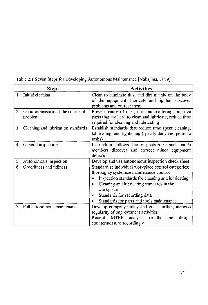
Table 2.1 Seven Steps for Developing Autonomous Maintenance [Nakajima, 1989]
Step Activities
1. Initial cleaning Clean to eliminate dust and dirt mainly on the body of the equipment; lubricate and tighten; discover
problems and correct them
Countermeasures at the source of
problem Prevent cause of dust, dirt and scattering; improve
parts that are hard to clean and lubricate; reduce time
required for cleaning and lubricating
Cleaning and lubrication standards Establish standards that reduce time spent cleaning; lubricating, and tightening (specify daily and periodic
tasks)
General inspection Instruction follows the inspection manual; circle
members discover and correct minor equipment
defects
Autonomous inspection Develop and use autonomous inspection check sheet
Orderliness and tidiness Standardize individual workplace control categories; thoroughly systemize maintenance control
e Inspection standards for cleaning and lubricating
e Cleaning and lubricating standards in the
workplace
e Standards for recording data
e Standards for parts and tools maintenance Full autonomous maintenance Develop company policy and goals further; increase
regularity of improvement activities
Record MTBF analysis. results and design
countermeasure accordingly
27

Table 2.2 Twelve Keypoints of Autonomous Maintenance [Tajiri, 1992]
Keypoints
1. Introductory
education
Description
Conduct thorough education which includes orientation and lecture
on TPM concepts prior to commencement of autonomous
maintenance activities
2. Cooperation among
departments
Promote maximum cooperation among _production-related
departments as well as administrative departments. Managers must
establish a support system for operators’ efforts.
3. Autonomous
maintenance is the
job!
All employees must recognize autonomous maintenance activity as
a mandatory part of operators’ routine jobs.
4. Small group — All activities must be developed based on small group.
5. Managers must take
the lead!
Front-line managers must take the lead and set an example to
demonstrate how to develop forthcoming steps of autonomous
maintenance program.
6. Education and
practice
Conduct thorough education and practice for operators without missing any minor opportunity.
7. Practice first Take breakthrough approach by way of thorough practice in order
to attain Zero Accidents, Zero Defects and Zero Breakdowns.
8. Actual effects Provide concrete subjects and targets for operators in terms of each
TPM activity, and encourage them to attain actual and effective
results.
9. Rules set by
operators The rules must be set by those who must follow them.
10. Autonomous
maintenance audit
The autonomous maintenance audit makes the largest contribution
toward encouraging and training PM groups.
11. Quick response The maintenance department must quickly and promptly treat work
orders from autonomous maintenance. If not, PM group activity
will certainly fail.
12. Be thorough Be thorough in developing each step of autonomous maintenance
program. If an audit is unsuccessful, do not proceed to the next
step in a hurry because of the schedule. When this happens, TPM
is not firmly implemented due to poor progress in technical
knowledge and skills.
28

specific subjects and goals are set within each subject. ZD groups, on the other hand, must
decide goals consistent with the company goals because the objective of ZD is to eliminate
defects and promote the achievement of all related goals. Although QC cycles and ZD small
groups differ organizationally, they often merge and interact with each other.
TPM small group activities are based on the ZD model and built into the
organizational framework. Specifically, TPM promotes autonomous maintenance by
operators through small group activities. In TPM, the typically management-directed activities
of equipment cleaning, inspection, etc., are performed as small group activities. The reason
why TPM small group activities should be integrated into an organizational structure is to
facilitate the top-down and bottom-up promotion of all information and requirements. Then,
small group goals can coincide with and be the same as company goals —- to improve
productivity and the work environment [Nakajima, 1988]. |
Experts’ experiences have indicated that success in small group activities depends on
three conditions: motivation; ability; and a favorable work environment [Nakajima, 1988].
Motivation and ability are the workers’ responsibilities. However, top management must take
the responsibility for actively promoting these three key factors. Its first responsibility is to
provide the necessary training and education to prepare a knowledgeable operator to perform
autonomous maintenance. Management’s second responsibility is to provide a favorable work
environment by eliminating environmental problems. TPM can not be successfully
implemented without the support of top management. Therefore, the function of top
management must thoroughly support small group activities.
2.3 Steps of TPM Development
The practical details and procedures necessary to develop a TPM program must be
tailored for each company individually. The program must be developed and adjusted to fit
individual requirements since needs and problems vary, depending on the company, type of
industry, techniques, production methods, and equipment conditions, from company to
29

company. Because of the variation in TPM development for each individual company, a
system development process, illustrated in Figure 2.3 [Blanchard, 1990], from the “system”
perspective, can be applied to enhance the development of TPM. An effective TPM program
begins with the definition of company goal/need and the analysis of system function. Then this
gives way to preliminary synthesis and allocation of requirement. The final stage is a trade-off
and optimization process. The application of system development process is useful for TPM
enhancement.
There are some basis conditions for the development of TPM that apply in most
situations. Generally, the minimum requirements for a successful TPM developed program are
summarized below [Nakajima, 1988]. These are also the fundamental TPM activities.
e Improving equipment effectiveness
e Autonomous maintenance by operators
e A planned maintenance program for the maintenance department
e Increased skills of operation and maintenance personnel
e An initial equipment management program
TPM is not a quick fix solution to a plant’s production equipment and maintenance
management problems. It takes two to three years for a full TPM implementation. The span of
TPM development can be divided into three stages. Table 2.3 lists the twelve basic steps of a
TPM development program [Nakajima, 1988]. In the preparation stage, an appropriate
environment has to be created by establishing a plan for the introduction of TPM. The
duration of preparation stage depends on the size of the company, level of technology,
management standards, and so on. Next, the implementation stage, the second stage, will take
two to three years to complete all implementation processes. During the final stabilization
stage, a plant must measure actual results accomplished against its TPM goals. Table 2.3 also
explains the methods of how to execute each step.
30

Definition of | | Need
1 . : oO ‘
Advance | System © Feasibility System rp Operational Studies
| Planning a | Requirements
S Technology
System Ly Development
Maintenance |. and pe
Concept Application = = Preliminary |
| System Analysis |
System Specification
___ Conceptual Design Review _ a
| System
Functional Analysis | |
. , foe
| Preliminary Synthesis | and *:
__ Allocation of Requirement __ |."
y
| |
| Trade-off and | Optimization i : !
| |
a NN S
“ os a“ NN
. > | _A7s Design Approach” No
oN Acceptable? Oe
Yes
|
| |
’ : | Synthesis and Definition Disapproval |
System Design Review & oe, TE ST fe
v
Approval
Figure 2.3 System Development Process [Blanchard,1990]

Table 2.3 The Twelve Steps of TPM Development [Nakajima, 1988]
p
Announce top
management decision to introduce TPM
Statement at TPM lecture in company;
articles in company newspaper
implementation and raise TPM levels
2. Launch education and Managers: seminars/retreats according
campaign to introduce to level
a TPM General: slide presentations
Preparation 3. Create organizations to Form special committees at every level an promote TPM to promote TPM; establish central
headquarters and assign staff 4. Establish basic and Analyze existing conditions; set goals;
policies and goals predict results 5. Formulate master plan for | Prepare detailed implementation plans
oe TPM development for the five foundational activities
“Preliminary: 6. Hold TPM kick-off Invite clients, affiliated and -implementation — subcontracting companies BS 7. Improve effectiveness of | Select model equipment; form project
each piece of equipment | teams 8. Develop an autonomous | Promote the Seven Steps; build
maintenance program diagnosis skills and establish worker
certification procedure TPM 9. Develop a scheduled Include periodic and predictive
implementation maintenance program for | maintenance and management of spare
oe the maintenance parts, tools, blueprints, and schedules
department 10, Conduct training to Train leaders together; leaders share
improve operation and information with group members
maintenance skill
11. Develop initial equipment | MP design (maintenance prevention);
management program startup equipment maintenance; LCC
analysis
_ Stabilization 12. Perfect TPM Evaluate for PM prize; set higher goals
32
Chapter 3
Measuring TPM Effectiveness
This chapter sketches the reasons for measuring TPM effectiveness and defines and
discusses the most basic and appropriate effectiveness measure in use — overall equipment
effectiveness (OEE). It also provides the process of a computerized model for OEE
calculation. The last section concludes with the countermeasures to eliminate equipment
losses.
3.1 TPM Effectiveness Measures
TPM is a continuous maintenance improvement program to eliminate equipment losses
and enhance equipment effectiveness. Effectiveness measurement is an important requisite of
the continuous improvement process. Problems impeding system output can be isolated and
the potential for improvement can be developed after effectiveness has been measured. The
measurement of TPM effectiveness makes it possible to find what causes losses and to look
for potential improvement. A measuring technique, which isolates the current problems and
predicts the potential for improvement, is necessary for each function and in each department
on a continuing basis over time in order to implement TPM program more effectively
throughout the company. In other words, the reasons for measuring TPM effectiveness are: to
help establish priorities for improvement projects, and to accurately and fairly reflect their
results [Nakajima, 1989].
A variety of indices showing effectiveness facilitate prompt identification of problem
and negative responses to change and facilitate more accurate judgment of the appropriate
countermeasures. Also, they help prompt more efficient implementation of TPM activities.
These measuring indices provide a close monitoring at all levels to help maintain and upgrade
33

implementation improvements, and to prompt the development of more effective
countermeasures to prevent sudden drops in effectiveness. Each company must decide which
indices are appropriate in its unique situation.
With increasing robotization and automation in current industrial environment,
productivity, cost, inventory, safety and health, and production output, as well as quality, all
depend on equipment. A measurement of effectiveness of equipment can accurately reveal
which areas are experiencing problems and the nature of those problems. Thus, the measure of
equipment effectiveness provides appropriate indicator for understanding and evaluating TPM
effectiveness. Equipment effectiveness is a measure of the value added to production through
equipment. The goal of TPM is to increase equipment effectiveness so each piece of
equipment can be operated to its full potential and maintained at that level.
The most basic and appropriate effectiveness measure related to equipment is overall
equipment effectiveness (OEE) [Nakajima, 1989]. It is extremely useful as an overall indicator
of factory or equipment performance. The detailed explanation and definition of OEE is
presented in section 3.2. Additionally, some effectiveness measures are used to measure the
preventive maintenance achievement rate, maintenance improvement rate, indices related to
PQCDSM (productivity, quality, cost, delivery, industrial hygiene and safety, moral), and so
on. Each rate or index used to measure TPM effectiveness has advantages and disadvantages.
Each company must decide the appropriate measure for its own environment and carefully
define the terms used. Moreover, the measurements selected must be meaningful to the people
who control them. All available data for calculating effectiveness should be correctly and
completely collected. Then the meaningful effectiveness measures can be used as a realistic
diagnostic measurement to evaluate TPM implementation. Overall equipment effectiveness is
selected as the effectiveness measure for this project.
34

3.2 Overall Equipment Effectiveness
Overall equipment effectiveness (OEE) is very much on the mind of TPM practitioners
these days. It is central to TPM scorekeeping and has become the plant standard for
improving to production processes. In TPM, overall equipment effectiveness encompasses all
of the operational and maintenance parameters to include availability, performance, and
quality. This shows that OEE incorporates the overall operating condition of the equipment
and thus leads to a more comprehensive, realistic measure of effectiveness. Developing a
customized version of OEE will help to maximize metric usefulness as an improvement index
and pinpoint equipment losses.
OEE represents the mathematical product of availability, performance rate, and quality
rate. The goal of TPM is to increase OEE. A high level of OEE can only be achieved when all
three effectiveness measures are high. The calculation and definition of the operating rate, the
performance rate, and quality rate are described as follows [Nakajima, 1988]:
1. Availability:
The operating rate (availability) is based on a ratio of operating time (excluding downtime)
to loading time. The mathematical equation is expressed as:
Loading Time— Downtime x 100%, Availability (operating rate) = Loadine Ti
oading Time
In this case, loading time is the daily (or monthly) operating time minus all forms of non-
operating time — breaks in the production schedule, stoppages for routine maintenance,
morning meetings, and other routine stoppages. Downtime means the total time taken for
stoppages such as breakdowns, retooling, adjustments, blade and drill bit replacement, and
SO ON.
2. Performance rate:
35

Performance rate is based on the operating speed and the net operating time. The operating
speed rate is the ratio of the initial speed of the equipment to its actual speed. In other
words, it shows the speed at which the equipment is actually operating relative to its ideal
speed. The equation used to define operating speed rate is:
Ideal cycle time Operating speed rate = x 100%
Actual cycle time
Net operating rate measures the maintenance of a given speed over a given period. The
formula for net operating time is as follows:
Processed amount x Actual cycle time x 100% Net operating rate = - 3
Loading Time — Downtime
Then the performance rate is calculated as follow:
Performance Rate = Operating speed rate x Net operating rate x100%
3. Quality rate:
The equation for quality rate is defined as:
. Pp ~ Def Quality rate = rocessed Amount — Defect Amount ~ 100%
Processed Amount
Figure 3.1 gives an example of a calculation of overall equipment effectiveness for
further clarification. The resulting OEE in this example is only 42.6% due to poor operating
speed rate and net operating time. This represents the average condition of most companies
before TPM implementation. Based on experts’ experiences, the ideal conditions are:
36

- Equipment Six big josses | Caiculation of overall equipment effectiveness
pmen loadi downtime | t oo, ing time — j Equipme Availability = 9 x 100
Loading time eg.) loading time
mins. — 60 muns. 2 Availability = 460 mins, ~ 60 mns. x 100 = 87%
Setup and 460 mins. | adjustment
iE Operating |= 3 3 time 136 idling and Performance _ theorencal cycie time x processed amount
oO munor stoppages efficiency operating time
(@.g.)
4 Performance - 0.5 mins./unit «x 400 units _
8 t Reduced efficiency 400 mins. x 100 = 50% Net ai speed
operating = time z
a 5 Defects in Rate of quality _ processed amount — defect amount process = x 100
o products processed amount 2 (e.g.}
Valuable a 400 units ~ 8 units operating | = 6 Rate of quaity_ avr x 100 = 98%
time g Reduced products 400 units
8 nw
Overaii t Pp stHlectivonose = Avatlability sthoweney Ce. Rate of quality products
(eg.) 0.87 x 050 x 0.98 » 100 = 42.6%
Figure 3.1 Example of OEE Calculation [Nakajima, 1988]
37

e Availability ... greater than 90%
e Performance rate ... greater than 95%
e Quality rate ... greater than 99%.
Therefore, the ideal for overall equipment effectiveness should be 85%
(0.90 x 0.95 x 0.99 x 100%), which is considered as world class and a benchmark to be
established for a typical manufacturing capability [Nakajima, 1988].
In practice, developing a universal calculation for OEE to match all applications of
TPM implementation has become more and more important issue [Kotze, 1993; Naguib,
1994]. Because manufacturing processes vary from industry to industry, plant to plant, and
even assembly line to assembly line, a generic OEE calculation, which clearly defines the terms
used in the OEE formula and completely relates to the operating logistic, current maintenance
practices, and the causes of losses, will be useful as an evaluating improvement tool
throughout manufacturing process. OEE applications vary depending on how the terms are
defined in the formula and how the data for inclusion and exclusion are selected. It is often
necessary to interpret all definitions to the people who use them, especially front-line
production and maintenance associates. Expert’s experience indicated that a consensus on five
key definition — planned downtime, unplanned downtime, machine cycle time, defect or yield
loss, and number of units produced during available time must be obtained in order to develop
a custom version OEE [Kotze, 1993]. The five key definitions are defined as follows:
1. Planned Downtime:
Planned downtime refers to “specially identified time during which available machinery is
not scheduled to produce product.” It includes scheduled breaks and lunches; scheduled
department or team meetings; and scheduled preventive maintenance, but does not include
changeovers; setups and adjustments; and startup time.
2. Unplanned Downtime:
38

Unplanned downtime refers to “any time during scheduled production that the machine is
not producing product.” It includes lost time due to breakdowns and failures; changeovers;
startup losses; recorded minor stoppages; setup and adjustments; and idling and waiting
time.
3. Machine Cycle Time:
Machine cycle time refers to “the engineering specified ideal or theoretical cycle time for a
specific machine, usually measured in minutes or fractions thereof.”
4. Defect/Yield Loss:
Equipment-related yield losses consist of product made during the measured period that is
scrapped or fails a quality check and must be reworked.
5. Number of Units Produced during Available Time:
It includes all units produced during the measured period which even includes startup and
ramp-down period, whether good, bad, or scrapped.
Ultimately, an agreement and consistency regarding which data are included or
excluded, the accuracy of the data, and the clear definition of each element used in the OEE
calculation are essential for a realistic, useful measure of overall equipment effectiveness.
Then, a real OEE value can actually evaluate the production losses being experiencing in the
factory. Unable to do these will mislead analysts to find out the real losses occurred in the
factory and to plan redundant countermeasures for the wrong causes of losses. Therefore,
using OEE as a diagnostic measure to improve equipment and process makes each TPM
implementer plan a profitable maintenance program and plan countermeasures against all
equipment losses.
3.3 Computerized OEE Model
Based on the definition and discussion of OEE parameters in section 3.2, a
computerized OEE model has been developed to measure the effectiveness of any equipment.
39
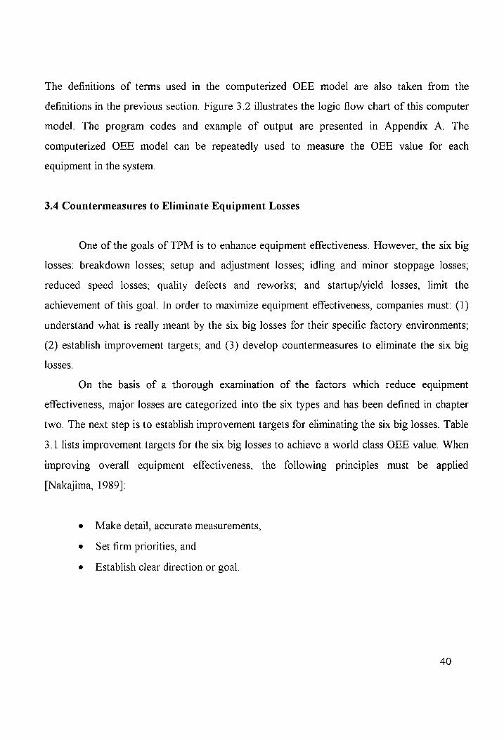
The definitions of terms used in the computerized OEE model are also taken from the
definitions in the previous section. Figure 3.2 illustrates the logic flow chart of this computer
model. The program codes and example of output are presented in Appendix A. The
computerized OEE model can be repeatedly used to measure the OEE value for each
equipment in the system.
3.4 Countermeasures to Eliminate Equipment Losses
One of the goals of TPM is to enhance equipment effectiveness. However, the six big
losses: breakdown losses; setup and adjustment losses; idling and minor stoppage losses;
reduced speed losses; quality defects and reworks; and startup/yield losses, limit the
achievement of this goal. In order to maximize equipment effectiveness, companies must: (1)
understand what is really meant by the six big losses for their specific factory environments;
(2) establish improvement targets; and (3) develop countermeasures to eliminate the six big
losses.
On the basis of a thorough examination of the factors which reduce equipment
effectiveness, major losses are categorized into the six types and has been defined in chapter
two. The next step is to establish improvement targets for eliminating the six big losses. Table
3.1 lists improvement targets for the six big losses to achieve a world class OEE value. When
improving overall equipment effectiveness, the following principles must be applied
[Nakajima, 1989]:
e Make detail, accurate measurements,
e Set firm priorities, and
e Establish clear direction or goal.
40
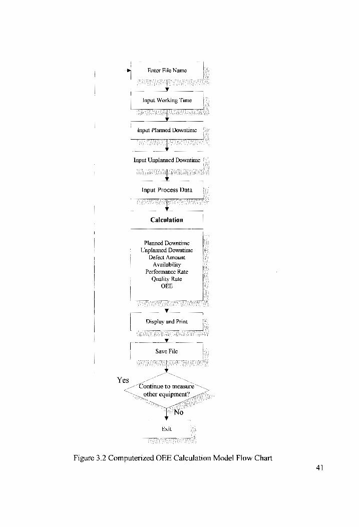
nd Enter File Name
Input Working Time
y
| Input Planned Downtime (
‘ —
| Input Unplanned Downtime |
| |
| ' Input Process Data L
-
Calculation
—
——
Planned Downtime
Unplanned Downtime Defect Amount
Availability Performance Rate
Quality Rate
OEE
OW
Display and Print /
y
Save File
= Yes
| “S Cnninue to ed
wether equipment” ee
I Exit
Figure 3.2 Computerized OEE Calculation Model Flow Chart
4]
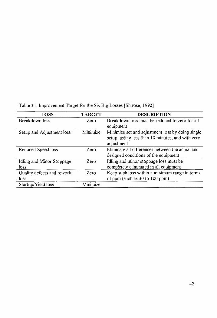
Table 3.1 Improvement Target for the Six Big Losses [Shirose, 1992]
LOSS TARGET DESCRIPTION
Breakdown loss Zero Breakdown loss must be reduced to zero for all equipment
Setup and Adjustment loss Minimize Minimize set and adjustment loss by doing single
setup lasting less than 10 minutes, and with zero
adjustment Reduced Speed loss Zero Eliminate all differences between the actual and
designed conditions of the equipment Idling and Minor Stoppage Zero Idling and minor stoppage loss must be loss completely eliminated in all equipment
Quality defects and rework Zero Keep such loss within a minimum range in terms
loss of ppm (such as 30 to 100 ppm)
Startup/Yield loss Minimize
42

Once OEE has been measured, a factory can determine its priorities for improving availability,
performance rate, or quality rate, and find the root causes of losses from the results of
OEE calculation. Then the factory can establish the specific improvement targets and develop
the countermeasures for eliminating all equipment losses for its own situation to increase
equipment effectiveness.
To reach the target of zero breakdowns, five countermeasures must be conscientiously
pursued. Neglect of any one or more than one of them can directly trigger a breakdown or
cause malfunction in equipment. The five countermeasures are[Tajiri, 1994]:
1. Establish the basic equipment condition
Adhere to the usage condition of operation
Restore deterioration
Correct design weakness
nA FY ON
Enhance operating and maintenance skills
Setup and adjustment downtime is the time required for stopping current production
and setting up for production of the next product. Setup and adjustment ought to be
performed quickly and accurately. Figure 3.3 presents a systematic improvement program to
minimize the setup and adjustment losses.
Idling and minor stoppages are caused by temporary problem in the equipment. Since
they can usually be restored quite simply, operators tend to overlook them and not regard
them as losses. However, this is a mistake and will cause a reduction in performance rate. The
zero idling and minor stoppage goal is essential. Figure 3.4 illustrates an overview of the
improvement program for reducing idling and minor stoppages.
A speed loss is the lost production caused by the difference between the designed
speed of a machine and its actual operating speed. Keeping the machine operating at the speed
set by the operating standard prevents this loss. Table 3.2 outlines a systematic improvement
program to eliminate the reduced speed losses. Losses incurred by rework and defect has a
43
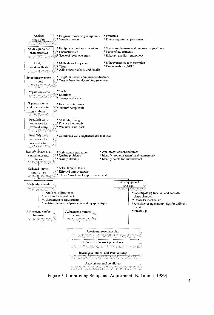
| Study equipment characteristics
Analyze ; | work methods
Setup improvement |
Separate internal
and external setup __operations
external setup
Establish work
| sequences for
internal setu
| Identify obstacles to
stabilizing setup
times __
i
Reduced internal
i © * Variable factors
- * Characteristics «“-* Scope of setup operation
* Methods and sequence - * Time
~s:* Adjustment methods and details
Preparatory steps .
Establish work | sequences for. :
. -2* Quality problems | °* Startup stability
* Problems
* Points requiring improvement * Progress in reducing setup times
* Shape, mechanism, and precision of jigs/tools * Scope of adjustments * Effect on ancillary equipment
* Equipment mechanism/system
* Effectiveness of each operation * Pareto analysis (ABC)
* Targets based on equipment restrictions | targets (.~* Targets based on desired improvement
* Tools
~-s* Locations
~ * Transport devices
_ * External setup work . * Internal setup work
* Methods, timing “* Practice thoroughly
-~* Workers, spare parts
* Coordinate work sequences and methods
* Attainment of targeted tumes * Identify problems (man/machine/method) * Identify points for improvement
* Stabilizing setup times
- * Select targeted tasks
setup times -» * Effect of improvements eeccoeens uoeeeroranees * Theme/direction of improvement work
~ . atm ste
djustment can be i . .
| eliminated L_
Study adjustments | -
| ~ * Details od adjustments * Reasons for adjustments
| * Alternatives to adjustments * Relation between adjustments and equipment/jigs
A
Study equipment
and jigs ps:
Investigate jig function and consider
shape changes * Consider mechanisms
* Consider using common jigs for different work
* Preset jigs
Adjustments cannot |
| be eliminated =F
Create improvement plan | ces — ee pee ee ee pS
z Establish new work procedures | a
Investigate internal and external setup
Ascertainoptimal conditions | ;
Figure 3.3 Improving Setup and Adjustment [Nakajima, 1989] 44
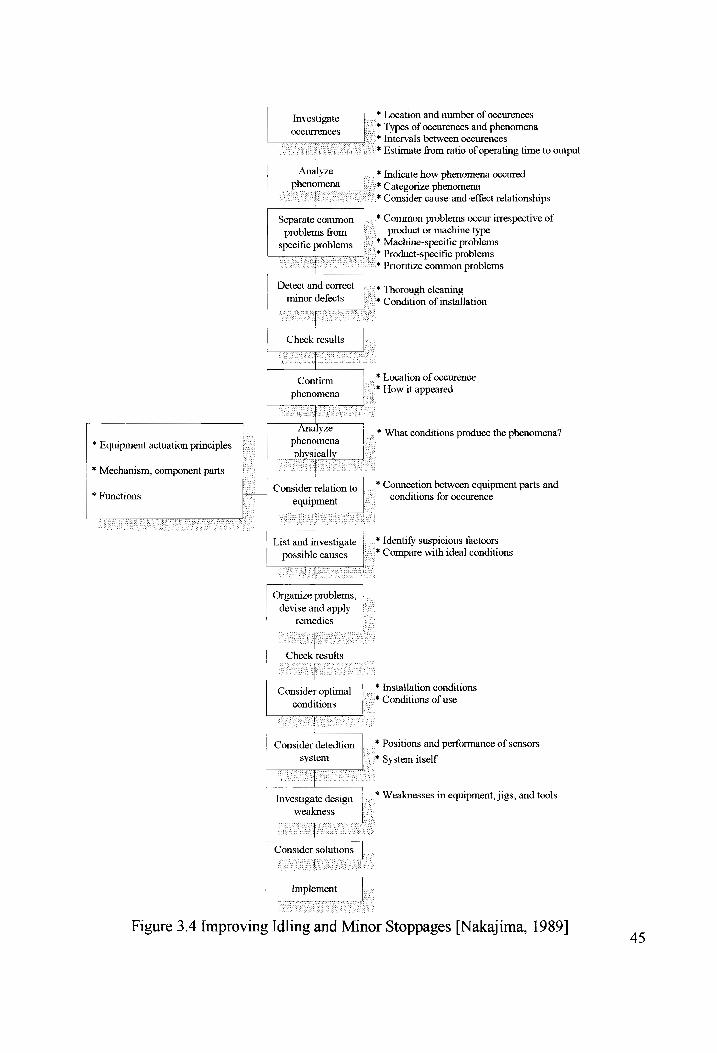
Investigate occurrences
SSS {
Analyze
Separate common
problems from specific problems
Detect and correct
minor defects
Confirm phenomena
phenomena :
Check results -
* Equipment actuation principles
* Mechanism, component parts
* Functions
Analyze
phenomena
| Consider relation to
equipment
List and investigate possible causes
_ physically _t
devise and apply | remedies
12
oe
1 OR
1
jorl:
, 1 4!
Consider optimal conditions
|
| Consider detedtion system
Investigate design
weakness
Organize problems, |
cas cera
Consider solutions
t Implement
_* Location and number of occurences ~ * Types of occurences and phenomena
-* Intervals between occurences
:* * Estimate from ratio of operating time to output
...* Indicate how phenomena occured
|, * Categorize phenomena -“. * Consider cause-and-effect relationships
-* Common problems occur irrespective of product or machine type
aot Machine-specific problems !=~* Product-specific problems -’* Prioritize common problems
~ * Thorough cleaning
.-.* Condition of installation SES
_* Location of occurence
’-"* How it appeared
_ * What conditions produce the phenomena?
* Connection between equipment parts and conditions for occurence
. * Identify suspicious factoors ‘:. * Compare with ideal conditions
* Installation conditions
..* Conditions of use
* Positions and performance of sensors
~ * System itself
_ * Weaknesses in equipment, jigs, and tools
Figure 3.4 Improving Idling and Minor Stoppages [Nakajima, 1989] 45
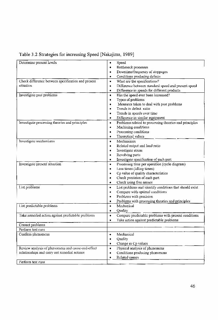
Table 3.2 Strategies for increasing Speed [Nakajima, 1989]
Determine present levels Speed Bottleneck processes
Downtime/frequency of stoppages Conditions producing defects
Check difference between specification and present situation
eo eeffneoe
@ @
What are the specifications? Difference between standard speed and present speed Difference in speeds for different products
Investigate past problems Has the speed ever been increased?
Types of problems Measures taken to deal with past problems Trends in defect ratio
Trends in speeds over time Difference in similar equipment
Investigate processing theories and principles Problems related to processing theories and principles
Machining conditions
Processing conditions
Theoretical values
Investigate mechanisms Mechanisms
Related output and load ratio
Investigate stress Revolving parts
Investigate specification of each part Investigate present situation Processing time per operation (cycle diagram)
Loss times (idling times) Cp value of quality characteristics
Check precision of each part
Check using five senses
List problems List problems and identify conditions that should exist Compare with optimal conditions
Problems with precision
Problems with processing theories and principles List predictable problems Mechanical
Quality Take remedial action against predictable problems Compare predictable problems with present conditions
Take action against predictable problems
Correct problems
Perform test runs
Confirm phenomena Mechanical Quality
Change in Cp values Review analysis of phenomena and cause-and-effect relationships and carry out remedial actions
Physical analysis of phenomena
Conditions producing phenomena
Related causes Perform test runs
46
huge impact on equipment effectiveness. Therefore countermeasures against it are among the
most important activities in an effort to eliminate the six big losses. Figure 3.5 provides a
continual improvement approach to achieve the zero defect target. Ultimately,
startup/yield losses refer to the losses that occur during the early stages of production — from
machine startup to stabilization. Such losses are latent, and the possibility of eliminating them
is often obscured by uncritical acceptance of their inevitability.
In addition, a variety of tools can be effectively applied throughout the life cycle in
accomplishing analysis, evaluation, and assessment tasks for a typical manufacturing system.
This, in turn, can provide the necessary additional support in maximizing OEE value.
For instance, reliability and maintainability assessments provide a quick measure of
equipment availability and the downtimes being experienced. P-M analysis promotes the
thorough and systematic elimination of defects. Through P-M analysis, all pertinent factors in
losses are efficiently identified [Nakajima, 1989]. Ishikawa’s cause and effect diagram, also
called the “fishbone diagram”, is a highly effective technique in delineating potential causes
responsible for a failure [Ishikawa, 1982]. The cause and effect diagram is used in the
FMECA to determine the causes responsible for the occurrence of any particular failure. The
failure mode, effects, and criticality analysis (FMECA) is an excellent tool which
systematically identify system failures, failure modes and frequencies, the effect of failures on
other elements of the system, criticality, and the need for possible preventive maintenance
[Blanchard, 1992]. It is a useful technique utilized during the conceptual and preliminary
design phase, and evolves through the detail design and development phase. The FMECA is
not only best used to enhance the equipment design and the corresponding support
infrastructure, but also used to evaluate and continuously improve existing equipment. The
objective of both cases is to increase overall equipment effectiveness, reduce maintenance and
support costs, increase productivity, and increase overall international competitiveness. The
reliability centered maintenance (RCM) is a systematic approach to develop a focused,
effective, and cost-efficient preventive maintenance program and control plan for a product or
process [Blanchard and Verma, 1995].
47
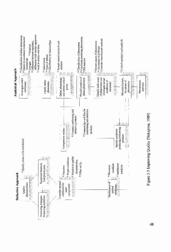
SOTIIATIOV soURUa}UIEA]
spoyjaul pue
sprepur)s JomUCD
, |
puawousyd Jo
sasneo Ioj
syutod JoTU09
ag
SPOU}OU JUAWOAINSLOUL
JOPISUO? » *
sUa|qold JO
S9OMOS JST
4: : BuauoUaYd
Jo sasneo
MATAOY »
SISATRUR JA 4.
euowouayd Buronpoid
suOT}IPUOZ) 4%’
BUsUOUAY
Jo UOTJBOTISSE[D
»
spotjow pue
splepuR)s [ONO
JASAlY y
adAyuoneoo] Aq
UOTROTISSET?) »
syoayap Jo
sadAy, y °°
SHUNT OOO,
+
SUI] JBA0
S}OaJap Ul
PUT] »
quauidinba Ie[Iuts
YIM saoussayip
“SaUTTPOBU UsaMyaq
SOUSIOTIIC] y
uonBURA y
JUS}TULIOIU /SNONUTJUOS)
saduaINDIO UI
SPUDIT, 4”!
BuatoUsYd Joayap JO
UOTJBOTISSE]D) y
saBeloAy yo»
gouamnos0 Jo
suorrpuos [enjor
o}e3T}soAur pue
euawousyd jo
gsneo yore
ATTUAp]
[6861 “ewrfeyxen]
Arend Sutroiduyy
¢'¢ ansry
sjonpoid
BUIUIOJUOS Bulonpold
SUOTIPUOS ATTUSP]
Busuiouayd joayjap
Jo sIsAyBue
yeorsAy
syonpoid
daTjOQJap pue
BuraLOyUOa Jo}
soip pue
sail aredwos ,
sjonpoid sanoajap
pue Suruu0yuoo
aredw0s
syutod [onUos
yuaLMS pue
euatuousyd yoayacq
|____}. ——
sarpnys oaljeredu0;)
pusuouayd
yogyap AULT)
soouamooo yoojap
ayes1jsaauy
yovoaddy peanAjeuy
poureyUreUl aq
Oo} sonjea AyTEN?)
y
WOnTpUoS
NTS
3 este
uontpuos [eumdo
ATBSSODON| jo
souvuayutey |
d> wo way
» soljsuajoereyo
Aytpenb 0} UOT
PAY» -
syusuodui09
ureul
JO} SuoTIpUOOD
“2} yeumdo
septsuoa
BPN
y
suonpuos Jadolg
SUOIJOUN y
SUOT}IPUOD BUISsAD0Ig
sa[drourid Burssas0lg
syed yuauodwuo7
suoljoury yuowidinby
S
ONSUoPOBIeYD
Aytyen?)
yavouddy sanonpeqg
48
Through use of the proper tools, TPM implementers will not only consider the
enhancements of equipment effectiveness in the design phase, but also identify the limitations
of improving equipment effectiveness in practice. Further, company can plan countermeasures
to improve equipment effectiveness by using these tools throughout the equipment life
cycle covering the phase of system design and development, system production/construction,
operation, utilization, sustaining support of the system, and system retirement/disposal.
49
CHAPTER 4
CASE STUDY
The objective of this chapter is to analyze and measure overall equipment effectiveness
for a hypothetical factory. First, the factory’s production process and its operational and
maintenance log are established and assumed. Then, the effectiveness and the total cost of this
production system is calculated as the baseline condition. Possible potential enhancements to
increase the OEE value and reduce the total cost are also discussed.
4.1 Hypothetical Factory Environment
The hypothetical factory environment is assumed here for application of the OEE
model. The major product in company XYZ is called product “A”. The production process
flow of product "A" has been illustrated in Figure 1.5. After assembling the raw materials of
product “A”, the product process continues with the incoming inspection, fabrication,
subassembly, and assembly activities. At the end of process, the inspection and testing is
executed to check and examine the quality of product "A". Finally, through the packing and
shipping activity, product "A" is packaged and transported to customers.
Company XYZ operates two shifts. The first shift works from 8 a.m. to 5 p.m., the
second shift works from 5 p.m. to 12 a.m.. During each shift period, one hour of break time is
provided to let employees have their lunch, dinner, and a rest. A group meeting lasting thirty
minutes for each shift, is held on each Monday to improve communications and encourage
suggestions to increase the productivity and effectiveness of the company. Company XYZ
implements a scheduled, time-based preventive maintenance program to reduce and detect
failures in advance. It is assumed that company XYZ already has implemented some of the
TPM activities such as small group activity.
50

The owners of company XYZ feel that the production system is not maximally
effective and productive. Performing a review and evaluation of the current production system
has become necessary. After company XYZ evaluated the entire production process based on
the past records, the results show that the overall equipment effectiveness (OEE) of the
production system is only around 50% and the cost of maintenance activities is almost 60% of
the total product cost, an unfavorable portion of the total product cost. This evaluation
indicates that the company experiences a very low production rate with high levels of
required maintenance.
4,2 Operational and Maintenance Records
Assessment of the performance and effectiveness of a system requires the availability
of operational and maintenance histories of the various elements. A formalized data
information feedback subsystem with the proper output defined early in the life cycle with the
development of operational requirements and maintenance concepts must be designed,
developed, and implemented to achieve this objective. The data information feedback
subsystem can provide the necessary data to evaluate and assess the performance,
effectiveness, operation, maintenance, and so on, for the system in the field. It also provides
historical data which can be applied in the design and development of new system having a
similar function and nature.
With realistic overall system requirements defined early in the design phase, the next
step is to identify the specific data factors which must be acquired and the method for
acquisition. Then, a format for data collection is developed to identify and collect the specific
factors and includes both success data and maintenance data. Success data, illustrated in
Table 4.1, constitute information including system operation and utilization on a day-to-day
basis. Maintenance data, listed in Table 4.2, include each scheduled and unscheduled
maintenance event [Blanchard, 1992]. The format for data collection must be compatible with
the systems in the factory. However, the data collection form should be easy to understand
51

Table 4.1 System Success Data [Blanchard, 1992]
System Operational Information Report
1. Report number, report date, and individual preparing report. 2. System nomenclature, part number, manufacturer, serial number.
3. Description of system operation by date (mission type, profiles and duration)
4, Equipment utilization by date (operating time, cycles of operation, etc.). 5. Description of personnel, transportation and handling equipment, and facilities required for
system operation. 6. Recording of maintenance events by date and time (reference maintenance event reports).
Table 4.2 System Maintenance Data [Blanchard, 1992]
Maintenance Event Report
1. Administrative data
(a) Event report number, report date, and individual preparing report. (b) Work order number.
(c) Work area and time of work (month, day, hour). (d) Activity (organization) identification.
2. System factors
(a) Equipment part number and manufacturer. (b) Equipment serial number. (c) System operating time when event occurred (when discovered). (d) Segment of mission when event occurred.
(e) Description of event (describe symptom of failure for unscheduled actions). 3. Maintenance factors
(a) Maintenance requirement (repair, calibration, servicing, etc.).
(b) Description of maintenance tasks.
(c) Maintenance downtime (MDT).
(d) Active maintenance times (Mct; and Mpt; ).
(e) Maintenance delays (time awaiting spare part, delay for test equipment, work stoppage,
awaiting personnel assistance, delay for weather, etc.). 4. Logistics factors
(a) Start and stop times for each maintenance technician by skill level.
(b) Technical manual or maintenance procedure used (procedure number, paragraph, date, comments on procedure adequacy)
(c) Test and support equipment used (item nomenclature, part number, manufacturer, serial number, time of item usage, operating time on test equipment when used).
(d) Description of facilities used. (e) Description of replacement parts (type and quantity).
i. Nomenclature, part number, manufacturer, serial number, and operating time on
replaced item. Describe disposition. i. Nomenclature, part number, manufacturer, serial number, and operating time on
installed item. 5. Other information
Include any additional data considered appropriate and related to the maintenance event.
52

and complete. The factors specified on each form must be clear and concise in terms of
application, and not require a lot of explanation and manipulation to obtain. The needed
measurement can be completed properly, and the right type of data can be collected.
Operational and maintenance records are the primary available sources to assess the
performance and effectiveness of a factory. Keeping them helps evaluate TPM effectiveness
and points out the enhancements necessary to eliminate the six big losses in TPM
implementation. Furthermore, it encourages a factory to plan countermeasures to decrease
losses and increase productivity and effectiveness. Thus, documenting operation and
maintenance is one of the most important activities in TPM implementation. The factors to be
considered and recorded in OEE evaluation have been identified and defined in Chapter Three.
When operational and maintenance records are properly collected and filled out, the factory
managers can figure out the OEE level and plan improvements to increase TPM effectiveness.
The formats for data collection and the types of records are not fixed, but are arranged
by management to dovetail with a particular plant’s requirements. The following types of
records, whose uses are summarized in Table 4.3, are minimally required in the practice of
TPM [Nakajima, 1989]:
1. Routine inspection records.
2. Lubricant replenishment and replacement records.
3. Periodic inspection records.
4. Maintenance reports.
5. Maintainability improvement records.
6. MTBF analysis records.
7. Equipment logs.
8, Maintenance cost records.
53
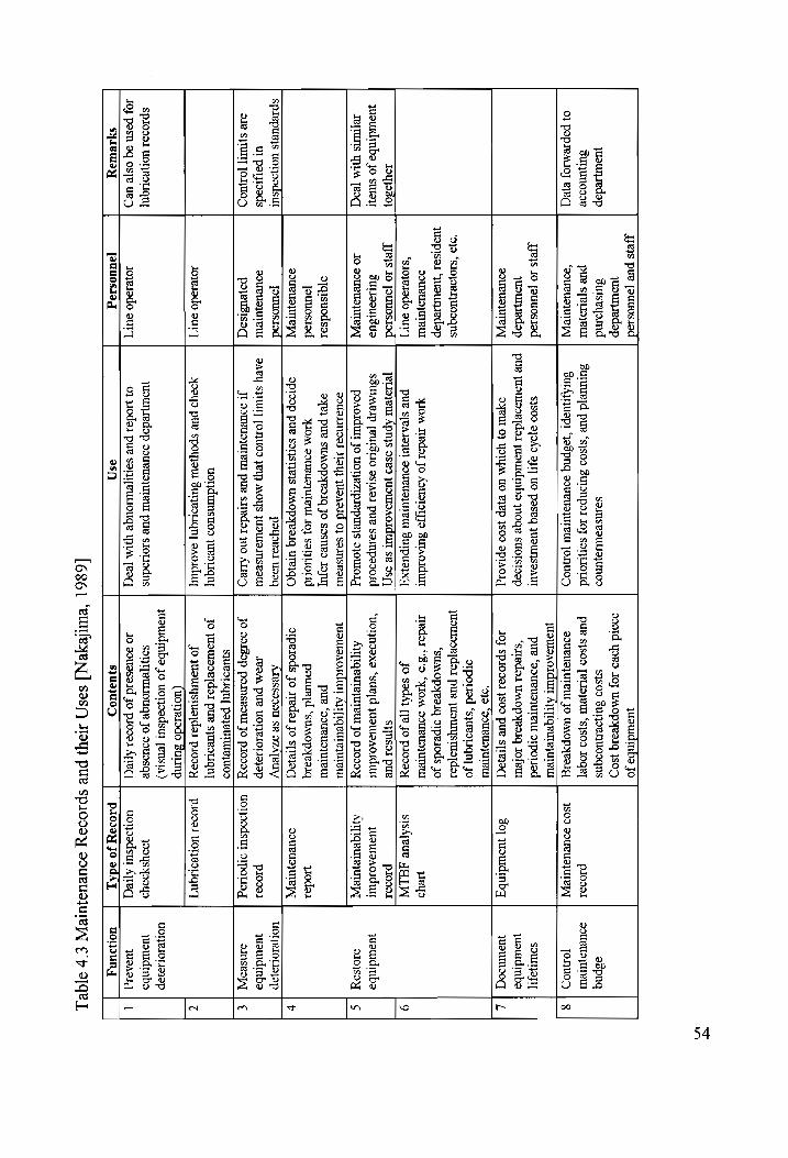
Jes pue
jauuosiod yusuidinba
jo yuounredsp
g001d yoed
IO} UMOpyPelg
1so_ yuourpredap
sutseyoind somMsPouL9}uNod
$}so00 SuT}OeNUODQNS
ospnq sutjunosoe
pue sjeusjeul
sutuueld pure
‘s}soo Sulonpal
Joy soquoud
pue s}sod
[eLIajeUr ‘s}sod
JOQR] psooel
| souPudjUTeUT
0} popreAloy
Bec] “‘QouBUaUTeY]
SUIAJIUApT “Jaspng
oUeUd}UTeUI [ONUOD
JouBUo}UTeUI JO
UMOpyeaig | S09
souRUaUTeY] JonUos
JUSUIDAOIduAT Ay] IqeuTeyUTeUr Jyeis
Jo Jauuosied
$}SO9 9[DA9
JI] UO
paseq JUSUTSOAUI
pure ‘90ueUd}UTeUI
sIpoLod SOUT}OIT]
yusurpedap | pur
juoulsoeydal yuouidnbs
ynoge suoIsIoep
‘srredai wnopyeeiq
Jofeul quowdinbo
sOUBUDdJUTBY] DYPUI
0} YOTYA
UO BYLP
SOD SPIAOIY
JO} SpJO9aI
}SOO pure
s]ie}3C] 30]
JUoUIdInbaz quauMs0q
‘Ojo “QouUBUO}UTeUI
oIpouiad ‘syuesLiqny Jo
‘OJo ‘sIO}OBUONQNS
quous0R|[do1 pue
yuourystuaydal JUaptIsal
‘Uouredop ‘suMOpyeelg
IIpesiods Jo
0UvUD IIe yom
Itedal Jo Aouatoyyjo
Sutaoiduit Jtedar
“3'd “YOM
soUvUD}UTeUI yey
“‘s10je1odo sur]
PUP S[PAIOJUL
SOURUIOJUTeU SUIpPUd}Xy
Jo sodA}
[]e Jo plosay
sisAjeue JGIW
131}930} eis
10 [ouUOsIod
[eUa}eur Apnjs
9SBd JUSUIDAOICUIT
SB osSy)
S$}[NSOI pue
Pp10991 yusuidinbo
jo surat
SULIZOUISUS SSULMBIP
[BUISUO SSIADI
puke sampooold
‘uolndexe ‘sued
yususAoldurt quoursaojdunt
quowdinba Jes
YUM [ead
Jo s0ueuayUTReY
poaoldunt Jo
UonezIprepurys sJOWOlg
Ajl[Iqeuteyuteul JO
p1090y Aytyiqeuteyureyy
310]S9Y
JUILINIOL IS}
JUSAIIG 0} SoMseoul
quouaaordunt AjTfiqeureyuteul
d][qIsuodsal dYe}
puv SUMOPYPLIIQ
JO SasneLd
JoJU] pue
‘soueusyUIeUl [ouuosiod
YOM sUeUDJUIeU
Jo} soruoUud
pouuryd ‘sumopyeoiq
yoda souBUaIUTeY]
oploop pur
sonsie)s Wnopyeelq
ule}qO oipeiods
jo Inedai Jo
s]tejoq JoUBUIa}UIEVY
Spiepuer}s uoTdedsut
jouuosiod payoeal
u90q ATessaoou
se aZzATeuy
UOT}BIOLII}ap ul
patjioods souBUa}UTeUL |
SAY S}IUT]
[O.UOD yey}
MOYsS JUSUOINSeaU
Jean pue
UOTPIOLIA}Op p10901
yusuidinba are
S}TUM] JONUOD
poyeusisaq Ji
soueuoyUTeUl pue
sitedal yno
Aud
jo soidop
poMseoul Jo
plossy |
UOTodsut sIpoLag
omseayy]
sjUBILIGN] poyeuTUTE}U0d
uondumsuos jueouqny
jo JuauIs0R
| dal pure
sjuP gn]
Joyexodo our]
YoY
pue Sspoyjsu
SuNeILIQn] sAcIdwy]
jo JUawystusydal
pilosay | psosel
uoT}ROUIQn’]
(uoleiodo suLinp
yuawadinbs Jo
uonsadsut [ensta)
uoT}BIOLIO}ap Splodal
Wore IUIQn] jUouTpedap
soueUajUTeUI pure
sioLiadns soljlTeuLoUqe
Jo souasqe
yooysyooyo yuowdinba
JO} posn
9q osje
ued Joyeiodo
Sur 0}
Podal pue
sonljeuuouge ILM
[ea] Jo
30uasald Jo
psosal ApIeq
uonoodsut Ayreq
WUDAIIg SYABWIDY
peuuo0si3g asp
$}U9}U07) paosay
jo adhT,
youn
[636]
‘eunleyen] sos¢
oy} pue
sploooy souvusqurIEpy
¢ yp
9IGe]
54
Each factory should design and arrange the particular formats of the above records to
properly monitor the maintenance of any equipment and provide the right types of information
for an ongoing assessment of operations. Based on the previous discussion of the principles
and importance of keeping records, a real world company must ask all employees to collect
and fill out the operational and maintenance records accurately in its standardized formats.
Currently, many companies have developed and implemented a computerized maintenance
management system (CMMS) to keep records and monitor labor and material costs, process
maintenance work orders, control spare parts and inventory, and track the maintenance
downtime [Wireman, 1986].
To apply the OEE model, the operational and maintenance records in the hypothetical
factory have to be assumed. In order to get the necessary hypothetical data, we assume that
a given period was spent on monitoring the production process and logging its hypothetical
output and minor disruptions that occurred. We also assume that the operational and
maintenance personnel kept and recorded all logbooks for the entire production process. The
assumed necessary data, including preventive maintenance downtime, setup downtime,
adjustment downtime, breakdown and failure downtime, etc., for applying the OEE model are
summarized in Table 4.4 ~ Table 4.8.
The break times in the production schedule and the time for group meetings have been
excluded from the operation time frame. In Table 4.4, working time means the total operating
time. In Table 4.5, assume the ideal and actual cycle time is obtained from the historical
operation data. In Table 4.6, 4.7, and 4.8, the data are summarized from the various operation
and maintenance records in the field. According to these assumptions and data, the baseline
OEE values of each function in the hypothetical factory can be evaluated by the computerized
OEE model developed.
55
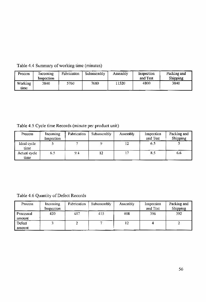
Table 4.4 Summary of working time (minutes)
Process Incoming Fabrication | Subassembly Assembly Inspection Packing and Inspection and Test Shipping _
Working 3840 5760 7680 11520 4800 3840 time
Table 4.5 Cycle time Records (minute per product unit)
Process Incoming Fabrication | Subassembly Assembly Inspection Packing and
Inspection and Test Shipping _
Ideal cycle 5 7 9 12 6.5 5
time Actual cycle 6.5 9.4 12 17 8.5 6.6
time
Table 4.6 Quantity of Defect Records
Process Incoming Fabrication | Subassembly Assembly Inspection Packing and
Inspection and Test Shipping |
Processed 420 417 415 408 396 392 amount
Defect 3 2 7 12 4 2
amount
56

Table 4.7 Summary of Downtime Records (minutes)
Process Incoming Fabrication | Subassembly Assembly Inspection Packing and
Inspection and Test Shipping _
Preventive 140 340 480 900 240 200 Maintenance
Setup _ 125 210 305 640 200 170 Adjustment 60 85 140 235 90 80
Changover 60 150 200 375 100 90
Breakdown 260 580 955 1580 385 365
& Failure Startup _ 120 165 180 285 145 160
Minor 30 120 200 215 100 65 stoppage Idling | 130 70 80 50 60 70
Table 4.8 Maintenance Action Records
Process Incoming | Fabrication | Subassembly | Assembly Inspection | Packing and Inspection and Test Shipping _
PM for facility 2 2 2 2 2 2
PM for equipment 2 2 2 2 2 2
CM for facility 2 6 8 12 4 3
CM for equipment 12 25 32 50 24 22
57

4.3 Effectiveness Evaluation and Analysis
An evaluation and analysis of effectiveness is performed to assess system performance.
The effectiveness of the hypothetical factory is evaluated and analyzed in this section. At first,
the initial assumed data are used to calculate the OEE values for each function block as the
baseline OEE values. The system OEE value is enumerated, based on the assumption of linear
relationship between each function block and the entire production process, by using the
system OEE model. Then, an analysis on the OEE parameters of function block is carried out
to seek possible improvements for increasing OFE value. In addition, since all factories aim to
make profits from production, a cost analysis must be performed to pinpoint the high cost
drivers in the factory and find reductions in the product costs. Thus, a cost analysis of the
hypothetical factory is also included in this section.
4.3.1 OEE Calculation
Overall equipment effectiveness presents a measure of the value added to production
through equipment. If there are problems and disruptions in production, the OEE measures
will be low. By using the OEE model described in Chapter Three and the hypothetical
operational and maintenance records, the OEE values are calculated for each function of the
production process. The results of calculating OEE for each function block in this case study
are summarized in Table 4.9. The detailed procedures of calculating OEE are given by the
example of OEE calculation in incoming inspection as follows:
Loading time = Working time - Preventive maintenance downtime
= 3840 - 140 = 3700 (minutes)
Operating time = Loading time - Unplanned downtime
= 3700 - 785 = 2915 (minutes)
58
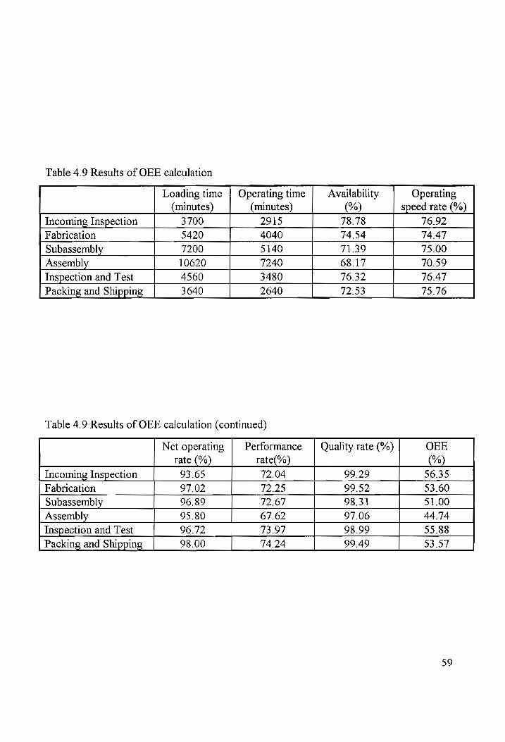
Table 4.9 Results of OEE calculation
Loading time | Operating time Availability Operating
(minutes) (minutes) (%) speed rate (%)
Incoming Inspection 3700 2915 78.78 76.92
Fabrication 5420 4040 74.54 74.47
Subassembly 7200 5140 71.39 75.00 Assembly 10620 7240 68.17 70.59
Inspection and Test 4560 3480 76.32 76.47 Packing and Shipping _ 3640 2640 72.53 75.76
Table 4.9 Results of OEE calculation (continued)
Net operating | Performance | Quality rate (%) OEE rate (%) rate(%) (%)
Incoming Inspection 93.65 72.04 99.29 56.35
Fabrication 97.02 72.25 99.52 53.60 Subassembly 96.89 72.67 98.31 51.00 Assembly 95.80 67.62 97.06 44.74
Inspection and Test 96.72 73.97 98.99 55.88
Packing and Shipping _ 98.00 74.24 99.49 53.57
59

Operating time Availability = x 100%
Loading time
_ 2915 3700
x 100% = 78.78%
Ideal cycle time per product unit x 100% Operating speed rate = : ; Actual cycle time per product unit
= x 100% = 76.92% 65
Processes amount x Actual cycle time Net operating rate = x 100%
Operating time
_ 420 x 6.5
2915 x 100% = 93.65%
Performance rate = Operating speed rate x net operating rate x 100%
= 0.7692 x 0.9365 = 72.04%
. Processed amount - Defect amount Quality rate = x 100%
Pr ocessed amount
417 x 100% = 99.29% 420
OEE = Availability x Performance rate x Quality rate x 100%
= 0.7878 x 0.7204 x 0.9929 = 56.35%
In the field, project teams constituted of production line supervisor and engineering
and maintenance staffs select equipment experiencing from the most serious equipment losses
and having the lowest OEE value for improvement. When positive results are achieved, the
project can be expanded to other similar equipment [Nakajima, 1989]. Then, the system OEE
value can be increased by the increasing the OEE value of each piece of equipment in the
system. Therefore, the individual OEE of each piece of equipment is more important and
useful in performing improvement activities of increasing equipment effectiveness rather than
60
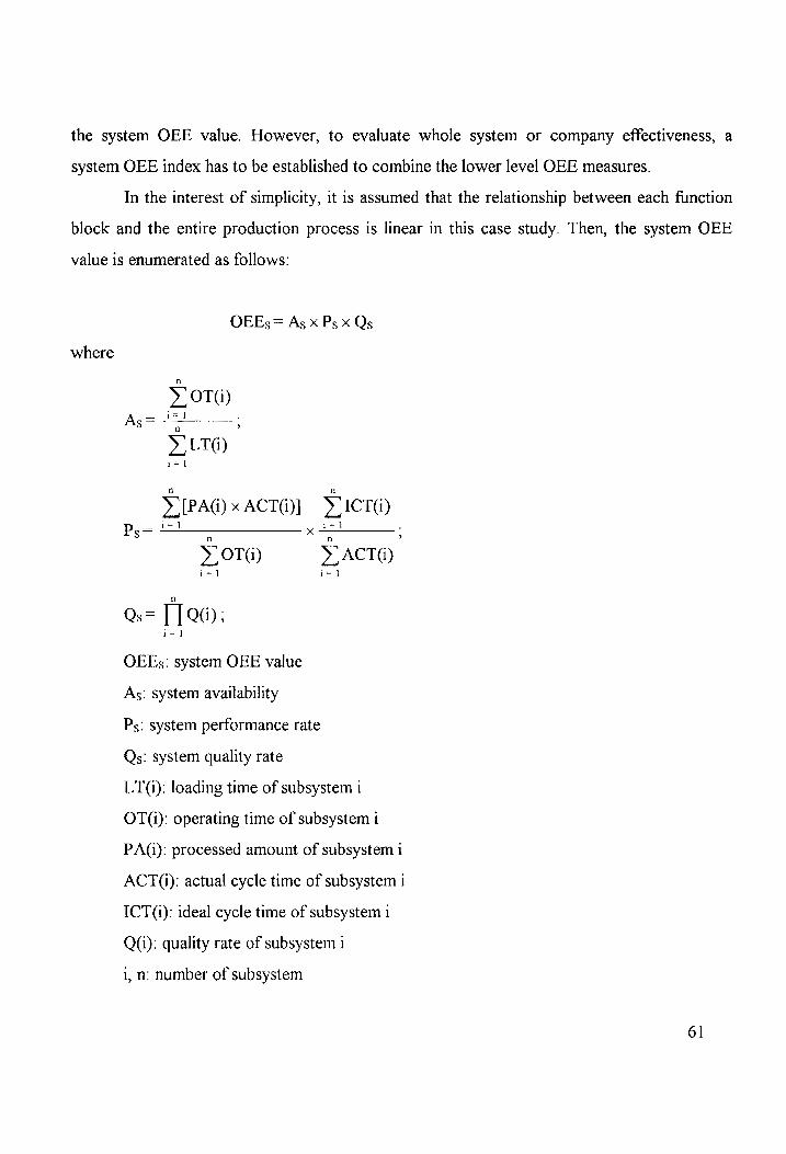
the system OEE value. However, to evaluate whole system or company effectiveness, a
system OEE index has to be established to combine the lower level OEE measures.
In the interest of simplicity, it is assumed that the relationship between each function
block and the entire production process is linear in this case study. Then, the system OEE
value is enumerated as follows:
OEEs = As x Ps x Qs
where
> OT()
Ag= +4 — )
> LT(G) i=]
Sy [PAG) x ACT(i)] x ICT(i) Py = i=} y te) ;
> OT(i) 5" ACT() |
Qs = [a0
OEEs: system OEE value
As: system availability
Ps: system performance rate
Qs: system quality rate
LTQ): loading time of subsystem 1
OT(i): operating time of subsystem i
PAQ): processed amount of subsystem 1
ACT@(): actual cycle time of subsystem 1
ICT(i): ideal cycle time of subsystem 1
Qi): quality rate of subsystem 1
1, n: number of subsystem
61

Since the system loading time is broken down into the loading time of each subsystem in the
whole system, the system loading time and the system operating time should be the sum of
those in each subsystem. Then, the formula of As can be defined as the ratio of the system
operating time to the system loading time. The actual cycle time for a product through the
whole system equals the sum of actual cycle time in each subsystem. Similarly, the ideal cycle
time for the system equals the sum of ideal cycle times of individual subsystems. Therefore,
the operating speed rate of the whole system is determined by the ratio of the summation of
subsystems’ ideal cycle time to the summation of subsystems’ actual cycle time. The net
operating rate of a system is defined as the system’s actual operating time divided by the
system’s operating time. It is obvious that the system operating time is the sum of the
operating time of each subsystem. The system’s actual operating time equals the summation of
actual operating times of each subsystem. Thus, the formula of Ps can be determined. The
quality rate is the probability of good products produced. It is assumed that the quality rates
of subsystems are independent of each other, 1.e., the quality rate of one subsystem is not
dependent on the quality rate of another subsystem. Consequently, for a series production
process, the system quality rate is the product of the individual quality rate of the subsystem in
the system. Consider a system OEE value in the production assembly process. When one or
more bottlenecks occur in the process, the idling downtime for the downstream processes
after the bottleneck is increased. Then, the system operating time is decreased because of the
more unplanned downtime. Therefore, the system availability and performance rate are
decreased, and, in turn, the system OEE value is also decreased.
At company XYZ, the OEEs of the hypothetical production process is calculated as
follows:
6
>> LT(i) = 35180 (minutes) i= |
6
>) OT(i) = 25455 (minutes) i= 1
62

6
> ICTG) = 44.5 (minutes per product unit) i=1
6
| ACT(i) = 60 (minutes per product unit) i=1
SIPAG) x ACT(i)] = 24519 (minutes) 1=1
25455 = >? _ 77 36%
As = 5180 °
, = ZANI8 449 _ 91 agp 25455. 60
Qs = Taw = 92.86%
OEEs = As x Ps x Qs = 48.00%
It shows the OEEs of the hypothetical factory is only 48.00% and there is a lot of room for
improvement to achieve the world class OEE value. The hypothetical factory can analyze the
OEE values to plan countermeasures for eliminating the factory’s losses.
4.3.2 OEE Analysis and Countermeasures
Performing analysis on parameters of OEE assists in the identification of which areas
in the factory are experiencing problems and what those losses are. Then, the countermeasures
to eliminate those problems and losses can be planned to increase the OEE values.
The previous OEE calculations for each function show that the low OEE value is
caused by the low availability and performance rate of each function, especially in assembly
function. Compared with the ideal conditions for a world class OEE value, the availability
which ranged from 68.17% to 78.78% and the performance rate which ranged from 67.62%
to 74.24 % are far away from the ideal conditions of greater than 90% and 95%, respectively.
63

To increase the OEE value of factory, the availability and the performance rate of each
function must be improved.
Availability is determined by the ratio of operating time to loading time. Assume the
loading time is fixed for the current factory environment, then the only way to increase the
availability is to reduce the unplanned downtime. According to the assumed operational and
maintenance data, breakdown and failure downtime is the highest contributor to the unplanned
downtime. To maximize availability, all breakdown and failure downtime must be reduced to
zero and the rest of unplanned downtime must also be eliminated. The impacts of respectively
increasing the availability of each function block on system OEE are presented in Figure 4.1.
These result from the assumptions of the performance rate and the quality rate of each
function block keep the same as the baseline conditions and the availability of one function
block is increased to 90%. For instance, in the assembly function, the improved OEEs results
from: (1) the loading times of each function block is fixed; (2) the operating times of other
function blocks are unchanged; (3) the performance rate and the quality rate of each function
block are the same as the baseline conditions; and (4) the availability of assembly is increased
to 90% by reducing the unplanned downtime. Then, the OEEs is computed by using the
system OEE formula and is presented as follows:
Loading time (assembly) = 10620 (minutes)
>| LT(i) = 35180 (minutes) 1=1
Operating time (assembly) = 10620 x 90% = 9558 (minutes)
>| OT(i) = 25455 — 7240 + 9558 = 27773 (minutes) i=]
277173 = =" = 78.95%
35180
Ps = 71.44%
Qs = 92.86%
OEEs = 0.7895 x 0.7144 x 0.9286 = 52.38%
64

OEEs
Incoming Inspection Subassembly Inspection & Test Fabrication Assembly Packing & Shipping
Function
Figure 4.1 Impacts of Availability on OEE (Availability = 90%)
65

Table 4.10 presents the detail results of this analysis for each function block. Actually, when
the availability is increased, the performance rate will be increased since the net operating rate
is increased by the reduction in the operating time for a certain quantity of product. Increasing
the availability of assembly function seems to have more influence on the system OEE value
because of its longer loading time. If the availability of assembly function is increased to 90%,
the system OEE will be increased to 52.38%. This is the largest impact of increasing the
availability on the system OEE among all function blocks. This analysis shows that increasing
the availability of assembly function results in the most significant improvement in enhancing
the system OEE.
Performance rate is the product of the operating speed rate and the net operating rate.
The net operating rate reflects losses resulting from minor stoppages. The operating speed
rate reflects reduced speed losses. In this hypothetical factory, low performance rates are
greatly caused by the low operating speed rate which ranged from 70.59% to 76.92%. In
order to improve the performance rate, idling and minor stoppage losses must be completely
eliminated in all equipment and all differences between the actual and ideal condition of the
equipment must be eliminated. Figure 4.2, which assumes (1) the loading time is fixed for the
current factory environment; (2) the net operating rate and the quality rate are unchanged; and
(3) the operating speed rate of one function block is increased to 90%, illustrates the impacts
of individually increasing the operating speed rate of each function block on the system QEE
after eliminating all idling and minor stoppage. Actually, by eliminating the idling and minor
stoppage, not only is the net operating rate increased, but also the availability is increased
because of the decrease in the unplanned downtime. The detailed outcomes of this analysis for
each function block are summarized in Table 4.11. For instance, the detailed procedures for
this analysis in assembly function are given as follows:
Loading time (assembly) = 10620 (minutes)
>, LT(i) = 35180 (minutes) i=1
66

Table 4.10 Results of OEE analysis for Availability
Function Loading time » LT(i) Operating > OT(i)
Time
Incoming Inspection 3700 35180 3330 25870
Fabrication 5420 35180 4878 26293 Subassembly 7200 35180 6480 26795
Assembly 10620 35180 9558 27773 Inspection and Test 4560 35180 4104 26079
Packing and Shipping 3640 35180 3276 26091
Table 4.10 Results of OEE analysis for Availability (continued)
Function As (%) Ps (%) Qs (%) OEEs (%)
Incoming Inspection 73.54 71.44 92.86 48.78
Fabrication 74.74 71.44 92.86 49.58 Subassembly 76.17 71.44 92.86 50.53
Assembly 78.95 71.44 92.86 52.38 Inspection and Test 74.13 71.44 92.86 49.18
Packing and Shipping 74.16 71.44 92.86 49.20
67

oe — ——_ ee
go -
75 |
70 —
60 |-
55 =
50 —
45 |-
40
35
OEEs
Incoming Inspection Subassembly Inspection & Test
Fabrication Assembly Packing & Shipping
Function
Figure 4.2 Impacts of Performance rate on OEE (Operating speed rate = 90%)
68

Table 4.11 Results of OEE analysis for Performance rate
Function Loading » LT(Q) Operating » OT(i) > ICT(i)
time Time
Incoming Inspection 3700 35180 3075 25615 44.5
Fabrication 5420 35180 4230 25645 44.5 Subassembly _ 7200 35180 5420 25735 44.5 Assembly 10620 35180 7505 25720 44.5 Inspection and Test 4560 35180 3640 25615 44.5
Packing and Shipping 3640 35180 2775 25590 44.5
Table 4.11 Results of OEE analysis for Performance rate (continued)
Function ACT » ACT(i) As Ps Qs OEE
(%) (%) (%) (%)
Incoming Inspection 5.56 59.06 72.81 72.57 92.86 49.07
Fabrication 7.78 538.38 72.90 73.42 92.86 49.90 Subassembly _ 10.00 58.00 73.15 73.90 92.86 50.20
Assembly 13.33 56.33 73.11 76.09 92.86 51.66 Inspection and Test 7.22 58.72 72.81 72.99 92.86 49.35
Packing and Shipping 5.56 58.96 72.74 72.69 92.86 49.10
69

Operating time (assembly) = 10620 — 3115 = 7505 (minutes)
6
>) OT(i) = 25455 - 7240 + 7505 = 25720 (minutes) i=]
= RTP = T311% 35180
6
> ICT(i) = 44.5 (minutes per unit product) +=]
Actual cycle time (assembly) = are 13.33 (minutes per product unit)
6
> ACT(i) = 60-17 + 13.33 = 56.33 (minutes per product unit) 1=1
Net operating rate (system) = 96.32%
44.5 Ps = 0.9632 x = 76.09%
56.33
Qs = 92.86%
OEEs = 0.7311 x 0.7609 x 0.9286 = 51.66%
Increasing the operating speed rate of each function block will increase the system OEE. It
results that the increase of operating speed rate in the assembly function has the largest impact
on the system OEE.
In a word, through previously performing the assessment and evaluation of OEE on
the current production process in the hypothetical factory, the causes of production losses can
be identified as follow:
1. In each function, the breakdown and failure downtime constitutes the largest part of
unplanned downtime and, in turn, significantly results in the low availability. Especially, in
the assembly function, 1580 minutes of breakdown and failure downtime contribute 47% of
unplanned downtime (3380 minutes) and cause the lowest availability among all function
70
blocks. The current preventive maintenance is not effective in preventing breakdown and
failure in advance.
2. According to the summary of downtime records, it is found that setup downtime constitutes
the averaged 29% of unplanned downtime excluding breakdown and failure downtime in all
function. This loss reduces the operating time and also reduces the availability of each
function.
3. The discrepancies between designed and actual speed of equipment in each function are so
distinct that the operating rates are low and the equipment is not operated at the designed
operating condition. These, in turn, cause the low performance rate. The largest distinction
between ideal and actual speed of equipment also occurs in the assembly function.
4. The lowest net operating rate among all function blocks is found in the incoming inspection
function. It represents that the incoming inspection function is experiencing the minor
stoppage and idling losses. According to the assumed operational and maintenance records,
the largest idling downtime is caused in the incoming inspection function. The reason may
be the insufficient supplies of raw materials. This, in turn, makes the incoming inspection
function have the second lowest performance rate among all functions.
5. Compared to the ideal condition for the quality rate which is greater than 99%, the quality
rates for most of the functions look good. However, the quality rates of around 97% and
98% are found in both subassembly and assembly functions. The reason for this loss is that
more amounts of defect products are produced in these two functions.
Once the causes of production losses have been identified, the company can recognize
the areas where improvement can be made to help increase the OEE value and the
productivity and plan countermeasures to eliminate those losses. The systematic improvement
program for eliminating the big losses described in chapter three can be applied here for
improving the OEFE value of the hypothetical factory. When planning the countermeasures, the
principle of setting the highest improvement priority to the assembly function because of its
71

largest impact on the system OEE must be emphasized. The countermeasures for the
hypothetical factory are recommended as follows:
1. Establish and maintain the basic equipment condition by three activities — cleaning,
lubricating, and bolt tightening. Then, maintain the equipment to be operated at its correct
condition and prevent and restore any deterioration occurring in the equipment. In the
mean time, the company must train operators and maintenance staffs to enhance their skills.
A review and upgrade of the current preventive maintenance is also necessary to detect and
predict the occurrence of equipment failure. By these activities, the breakdown can be
eliminated.
2. Study and analyze the setup data and work method in each function. Identify obstacles to
stabilize setup times. Separate the internal and external setup and convert internal to
external setup as much as possible. Then, the setup downtime can be minimized.
3. Investigate the processing theories, principles, and present operating situation. Identify the
possible causes of reducing operating speed. Predict the remedial action against the
possible obstacles. Take actual remedial action to eliminate the difference between the
designed and actual speed of equipment.
4. Analyze the phenomena of minor stoppage and idling. Detect and correct all minor
stoppages. Identify the bottleneck in the process and schedule the production process to
avoid the idling; especially, the supplies of raw materials in this process must be compatible
with the operating schedule of the incoming inspection function.
5. Investigate the defect occurrence to clarify defect phenomena. Analyze the defect
phenomena to set control points for causes of phenomena. Then, upgrade the
manufacturing process to eliminate such quality defect losses.
72
4.3.3 Total Cost Analysis
Since cost is a major parameter for evaluating system performance, it 1s necessary to
address cost in the effectiveness evaluation and analysis. In order to accomplish a total cost
analysis, a cost breakdown structure showing the numerous categories that are combined to
provide the total cost must be developed. In this case study, the total cost value involves
revenues and product cost category. The product cost category is broken down on a
functional basis, into investment, operations, maintenance, and material disposal/phase-out
subcategories as shown in Figure 4.3. The purpose of performing this total cost analysis is to
increase profit by minimizing product cost. In order to decrease product cost, the high cost
drivers must be identified and then the possible solutions to prevent those cost drivers should
be introduced.
In an attempt to simplify the problem and be compatible with the assumed operational
and maintenance records, this total cost analysis is performed for a given period and the
following additional data are assumed:
1. To calculate the revenues, the sale price of product A is $1,000 per unit.
2. Capital equipment costs, such as the cost of new, expended, replaced, or revamped
equipment, are $2,200 for the monitoring period.
3. The costs of computer resources, facilities, and data/documentation subcategories are
assumed on the basis of a given period. They are $632, $1,000, $740, respectively.
4. Spare/repair parts are required on the facilities and equipment for replacement of the units
that need repair. Assumed costs of spare/repair parts are determined by the maintenance
actions. It costs $32 per preventive maintenance action and $105 per corrective
maintenance action for the facilities. On the other hand, it costs $80 per preventive
maintenance action and $185 per corrective maintenance action for the equipment. This
cost includes material costs and inventory maintenance costs. The turnaround time on
spares is ignored for the sake of simplicity.
73
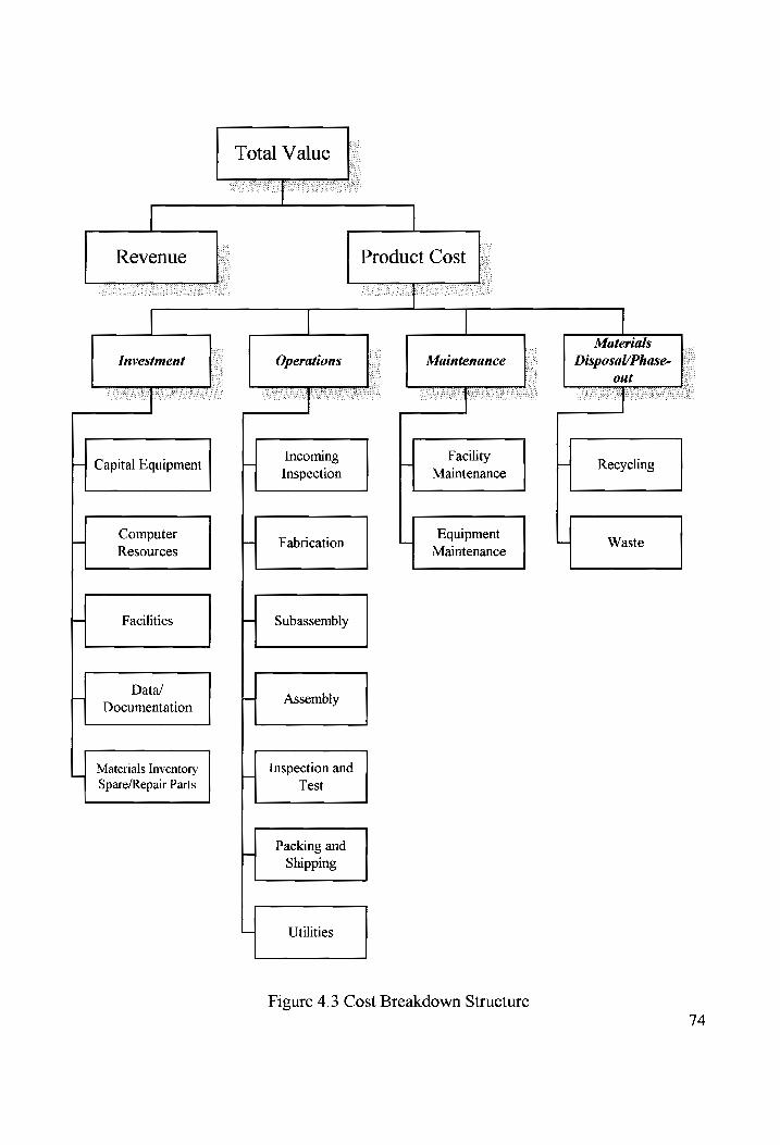
Total Value
Revenue |[* Product Cost
| 7 LC Materials S
Investment }- Operations |. Maintenance |- Disposal/Phase- |*- s : - out =
-— Capital Equipment Incoming 7 Facility - Recyclin: P quip a Inspection Maintenance young
—J Computer —) Fabrication — Equipment — Waste Resources Maintenance
— Facilities —| Subassembly
Data/
Documentation . Assembly
Materials Inventory Inspection and Spare/Repair Parts Test
L Packing and
Shipping
— Utilities Figure 4.3 Cost Breakdown Structure
74

5. The costs of operation category are allocated to unit product for each function of the
process. This includes the tooling and operation personnel cost. The associated costs of
each function is the following:
e Incoming Inspection: $10/unit
e Fabrication: $24/unit
e Subassembly: $36/unit
e Assembly: $55/unit
e Inspection and Test: $18/unit
e Packing and Shipping: $20/unit
e Utilities: $6.4/unit
6. In this case study, the maintenance activities can be primarily divided into performing on
both facility and equipment. Assume that the maintenance costs are based on the
maintenance actions performed. For the facility maintenance, it costs $145 per preventive
maintenance action and $500 per corrective maintenance action. For the equipment
maintenance, it costs $235 per preventive maintenance action and $870 per corrective
maintenance. This includes the costs for system maintenance and support and the
maintenance personnel costs.
7. Assume that the recycling and waste cost is $30 and $15 per unit, respectively.
From the assumed operational and maintenance records, process data, and the above
assumption of cost estimation, the total cost analysis can be performed. The revenue of
company XYZ is $390,000 and the total cost is $287,390 for the given period. This make a
profit of $102,610. The detailed product cost is presented as follows:
e Revenue = Sale price of product A x Amount of good product
= $1,000 x 390 = $390,000
e Cost of material inventory spare/repair parts
75
= $ per PM action x PM action + $ per CM action x CM action
Table 4.12 shows the results of this cost category for both facility and equipment.
e In operation cost category, the cost of each function is determined by the cost per unit
times the processed amount. For example, in the incoming inspection function:
Operation cost in incoming inspection function = $ per unit x processed amount
=$10 x 420 = $4,200
e For both facility and equipment,
Maintenance cost = $ per PM x PM action + $ per CM x CM action
The maintenance costs of both facility and equipment are illustrated in Table 4.13.
e In material disposal/phase-out cost category, the recycling cost is computed by the
recycling cost per unit times the number of good product and the waste cost is determined
by the waste cost per unit times the number of defect product.
The total cost breakdown of company XYZ for the given period is presented in Table 4.14. It
indicates that the maintenance cost, which constitutes 57.6% of total product cost, acts as the
highest contributor of the product cost. Meanwhile, from Table 4.12 and 4.13, the costs of
spare/repair parts and maintenance costs in the assembly function contribute above 30% of
subtotal costs of each cost category. It shows that the costs spending on the assembly function
are the highest cost driver of total product costs. Because both spare/repair part and
maintenance costs are associated with maintenance activities, performing a reevaluation on the
current maintenance approach is necessary. According to these cost analyses, analysts should
review and update the current maintenance approach to minimize the occurrence of failure and
breakdown and reduce the costs associated with the maintenance activities. Thereby, the
revenue can be increased, the total product costs can be decreased, the profit can be
substantially increased, and the OEE value can be improved. Furthermore, a cost-effectiveness
analysis can be performed to make a trade-off between the effectiveness of maintenance
approach and the total cost.
76

Table 4.12 Costs of Material inventory spare/repair parts ($)
Process Incoming Fabrication Subassembly Assembly Inspection and Packing Total Inspection Test and Shipping
Facility 244 694 904 1324 484 379 4029
% 6.1 17.2 22.4 32.9 12.0 9.4 100 Equipment 2380 4785 6080 9410 4600 4230 31485
% 7.6 15.2 19.3 29.9 14.6 13.4 100
Table 4.13 Maintenance costs ($)
Process Incoming Fabrication Subassembly Assembly Inspection and Packing Total Inspection Test and Shipping
Facility 1290 3290 4290 6290 2290 1790 19240
% 6.7 17.1 22.3 32.7 11.9 9.3 100
Equipment 10910 22220 28310 43970 21350 19610 146370
% 7.5 15.2 19.3 30.0 14.6 13.4 100
77
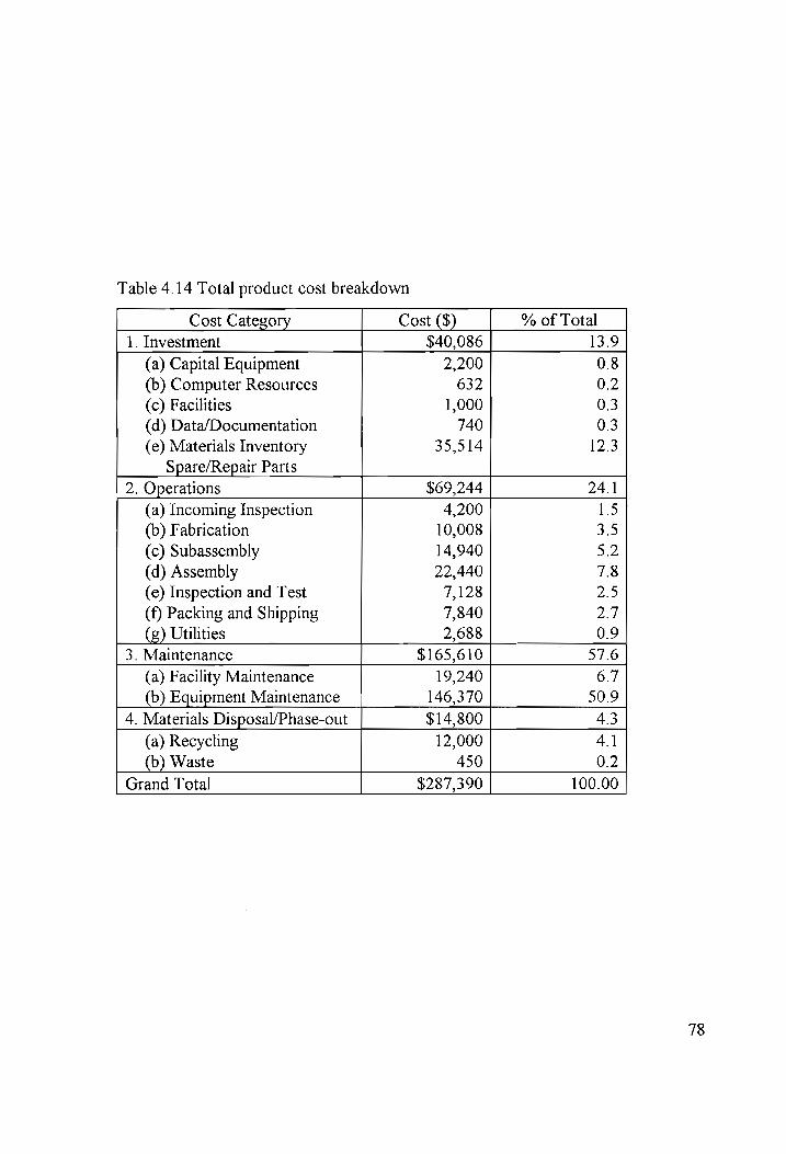
Table 4.14 Total product cost breakdown
Cost Category Cost ($) | % of Total 1. Investment $40,086 13.9
(a) Capital Equipment 2,200 0.8 (b) Computer Resources 632 0.2
(c) Facilities 1,000 0.3
(d) Data/Documentation 740 0.3
(e) Materials Inventory 35,514 12.3
Spare/Repair Parts
2. Operations $69,244 24.1
(a) Incoming Inspection 4,200 1.5
(b) Fabrication 10,008 3.5
(c) Subassembly 14,940 5.2
(d) Assembly 22,440 7.8
(e) Inspection and Test 7,128 2.5
(f) Packing and Shipping 7,840 2.7
(g) Utilities 2,688 0.9
3. Maintenance $165,610 57.6
(a) Facility Maintenance 19,240 6.7
(b) Equipment Maintenance 146,370 50.9
4, Materials Disposal/Phase-out $14,800 43
(a) Recycling 12,000 4.1
(b) Waste 450 0.2
Grand Total $287,390 100.00
78
4.3.4 Cost-Effectiveness Analysis
Cost-effectiveness relates to the measure of the hypothetical production system in
terms of OEE and total product cost. The objective of cost-effectiveness analysis is to balance
both the necessary technical and performance requirement related to the equipment operation
and maintenance and the total product cost in order to maximize the OEE value and profit
at a minimum total product cost. In this case, the specific cost-effectiveness figure of metric
(FOM) can be expressed as:
FOM = OEE
Total Product Cost
The FOM of company XYZ for the given monitoring period 1s:
FOM = _ 048 _ 1.6702 x 10° ~ $287,390
During the “continue improvement” approach for the TPM implementation, analysts can
evaluate the FOM value of improving maintenance approach to make a decision on
implementing what kind of enhancing maintenance approach to use. If one new maintenance
approach can increase the OEE value, reduce the total product cost, and, in turn, increase the
FOM value, this maintenance approach should be implemented to upgrade the current
maintenance approach. However, if one maintenance approach can increase the OEE value
but significantly increase the total product cost, the FOM value will be decreased. From the
cost-effectiveness standpoint, it is not an effective maintenance approach. In the hypothetical
factory, any maintenance approach which provides the FOM value greater than the baseline
FOM value (1.6702 x 10°) will be an enhancing maintenance approach. Thus, the greater
FOM value represents the more cost-effective approach and is preferred. Cost-effectiveness
79

analysis provides an excellent decision-making analysis to evaluate all alternative maintenance
approaches. It is believed that the FOM value will be increased after implementing TPM
program.
80

CHAPTER 5
SUMMARY AND FUTURE RESEARCH
This chapter presents a summary from this project and report. The future research for
this project and report is also suggested in this chapter.
5.1 Summary
This project has focused on the new integrated maintenance approach — “Total
Productive Maintenance (TPM)”. The concept of TPM and the steps of TPM implementation
have been presented, a specific measure of TPM effectiveness —- overall equipment
effectiveness (OEE) — has been defined, measured, and analyzed, and a computerized OEE
model has been developed to measure the OEE value for a given manufacturing system. The
countermeasures for eliminating the six big losses defined in TPM have been discussed to
improve availability, performance rate, and quality rate. Application of the OEE measurement
is illustrated through a case study assuming a hypothetical factory to measure the OEE value
by applying the defined OEE model, analyze the production losses from the OEE value, and
plan the possible countermeasures to prevent production losses. The computerized OEE
model has been used to calculate the OEE value for each function block in the hypothetical
production process. The cost-effectiveness approach using the total product cost and OEE
value has also been illustrated through the case study.
TPM is an integrated life-cycle approach to factory maintenance and support. The
complete implementation of such maintenance approach will lead to increased efficiency and
greater productivity for any given manufacturing system. Throughout the introduction of
TPM, the characteristics and the development steps of TPM can be completely realized and
the implementation can be employed in every department at every level of factory. Overall
81

equipment effectiveness is an important measure of TPM effectiveness. It involves all of the
Operation and maintenance parameters: availability; performance; and quality to evaluate the
overall operating condition of equipment. Availability indicates breakdown losses and setup
and adjustment losses. Performance rate shows speed losses and minor stoppage and idling
losses experienced in equipment. Quality rate points out quality defects and reworks losses
and startup losses. The evaluation of OEE value provides a measurement to investigate the
current maintenance approach and to assess the effectiveness of improving maintenance
approach. Moreover, from the OEE value, all production losses can be identified to lead to
plan countermeasures to eliminate those losses, and then the effectiveness and performance of
factory can be improved.
A hypothetical factory experiencing low OEE value and high maintenance cost is used
as a case study to perform OEE calculation, OEE analysis, total cost analysis, and cost-
effectiveness analysis. By applying the assumed operational and maintenance records into the
OEE model, the OEE value of company XYZ is only 48%. It shows that there is a lot of room
to improve the current maintenance approach at company XYZ. The OEE analysis for
availability and performance rate is performed to establish the priority of improving approach,
identify the causes of production losses, and plan the possible countermeasures to eliminate
production losses. It is found that the improvement of availability in assembly function block
has the largest influence on the system OEE value. Therefore, company XYZ should set the
highest priority to improve the availability of assembly function and plan the countermeasures
to eliminate the causes of affecting the availability of assembly function. The total cost analysis
on company XYZ indicates that the cost associated with maintenance activities (especially, the
maintenance cost in assembly function) are the cost driver for the total product cost of
product “A”. To reduce the total cost of product “A” and increase the profit of company
XYZ, the occurrences of equipment failure and breakdown must be eliminated to reduce the
maintenance costs. A specific cost-effectiveness figure of metric is expressed as the ratio of
OEE value to the total product cost in this case study. The current FOM value is 1.6702 x 10°
at company XYZ. Analysts can use this FOM value as a index to evaluate the FOM value of
82
improving maintenance approach to make a decision on implementing what kind of enhancing
maintenance approach. |
The objective of studying and analyzing the measurement of TPM effectiveness has
been met in terms of OEE. The analysis on factors affecting OEE value negatively has been
achieved by understanding the relationship between six big losses and OEE value. The
developed computerized OEE model has enabled OEE calculation more quickly. The
suggested countermeasures for the hypothetical factory has been planned from the OEE
calculation and analysis.
5.2 Future Research
TPM approach has been widely implemented around the world. Although the major
fundamental development steps of TPM have been established, companies intending to
implement TPM must “tailor” the current approach to be compatible. There are several ways
to further improve the work in this project and report. These include:
1. Apply the principles of implementing autonomous maintenance, the steps of TPM
development, the countermeasures of eliminating six big losses in a real factory to
establish the practical approach of those concepts and steps and understand how they
work in the field.
2. Integrate some system design methods such as failure mode, effects, and criticality analysis
(FMECA), reliability centered maintenance (RCM), and so on, into the activities of TPM
implementation to create an effective realistic implementation approach.
3. Apply the OEE model in a real factory to present how the OEFE value assist in evaluating
the effectiveness of maintenance approach and identifying the current experiencing losses
in the factory.
4. Establish a system OEE evaluation model to measure the OEE value for the different
configuration of manufacturing system.
83
5. Expand the model to consider additional system parameters from the logistics perspective
in order to achieve an optimal balance among those system parameters and life-cycle cost.
6. Expand the developed computerized OEE model to perform OEE evaluation and analysis,
and combine with the life-cycle cost analysis for the purpose of diagnosing and evaluating
the cost-effectiveness of maintenance approach.
7. Develop an expert system to integrate operational and maintenance figures, OEE
calculation, OEE analysis, life-cycle cost, etc. throughout the life cycle of equipment in the
factory.
84

REFERENCES
1. [Blanchard, 1969]
Blanchard, B. S. and E. E. Lowery, Maintainability Principles and Practices, McGraw-
Hill Book Company, New York, NY, 1969.
2. [Blanchard and Fabrycky, 1990]
Blanchard, B. S. and W. J. Fabrycky, System Engineering and Analysis, 2nd Ed.,
Prentice Hall, Englewood Cliffs, N. J., 1990.
3. [Blanchard, 1992]
Blanchard, B. S., Logistics Engineering and Management, 4th Ed., Prentice Hall,
Englewood Cliffs, N. J., 1992.
4. (Blanchard, 1994]
Blanchard, B. S., An Enhanced Approach for Implementing Total Productive
Maintenance(TPM) in the Manufacturing Environment, The Society Of Logistics
Engineers (SOLE), Hyattsville, MD., March, 1994.
5. [Blanchard and Verma, 1995]
Blanchard, B. S., Dinesh Verma, and Elmer L. Peterson, Maintainability: A Key to
Effective Serviceability and Maintenance Management, John Wiley & Sons, Inc., New
York, N. Y., 1995.
6. [Habayeb, 1987] Habayeb, A. R., System Effectiveness, Pergamon Press, Headington Hill Hall, Oxford,
England, U. K., 1987.
7. (Ishikawa, 1982]
Ishikawa, Kaoru, Guide to Quality Control, 2nd rev., English Ed., Asian Productivity Organization, Tokyo, 1982.
8. [Kotze, 1993]
Kotze, D., Consistency, Accuracy Lead to Maximum OEE Benefits, TPM Newsletter,
Vol. 4, No. 2, November 1993, AITPM, Productivity, Inc., Norwalk, Connecticut, 1993.
9. Koelsch, James R., A Dose of TPM, Manufacturing Engineering, pp. 63-66, April, 1993.
85
10.
11.
12.
13.
14.
15,
16.
17,
18.
19.
20.
[Mundel, 1983] Mundel, Marvin E., Improving Productivity and Effectiveness, Prentice-Hall, Inc.,
Englewood Cliff, NJ, 1983.
[Mobley, 1990]
Mobley, R. K., An Introduction to Predictive Maintenance, Van Norstrand Reinhold,
New York, 1990.
[Naguib, 1994]
Naguib, Hussein, On the Calculation of OEE and its Application in Semiconductor Equipment, TPM Newsletter, Vol. 4, No. 8, May, 1994, AITPM, Productivity, Inc.,
Norwalk, Connecticut, 1994.
[Nakajima, 1988]
Nakajima, S.. 7PM: Introduction to TPM, Combridge, MA., Productivity Press, Inc.,
1988.
[Nakajima, 1989]
Nakajima, S., TPM Development Program, Combridge, MA., Productivity Press, Inc.,
1988.
[Nieblel, 1994]
Nieblel, B. W., Engineering Maintenance Management, 2nd Ed., Marcel Dekker, Inc.,
New York, NY 1994.
[Shirose, 1992]
Shirose, Kunio, 7PM for Workshop Leaders, Combridge, MA., Productive Press, Inc.,
1992.
[Tajiri, 1992] Tajiri, Masaji and Fumio Gotoh, TPM Implementation: A Japanese Approach, McGraw-Hill, Inc., New York, NY, 1992.
[ Wireman, 1986]
Wireman, T., Computerized Maintenance Management Systems, Industrial Press, Inc.,
New York, NY, 1986.
[Wireman, 1992]
Wireman, T., Inspection and Training for TPM, Industrial Press, Inc., , NY , 1992.
[Wireman, 1994]
Wireman, T., Total Productive Maintenance: An American Approach, Industrial Press,
Inc., New York, NY, 1994.
86
BIBLIOGRAPHY
. Charles, Van Tine "Buck" L., TPM in the New Organization, Proceedings, Third
Annual Total Productive Maintenance Conference and Exposition, pp. 295-315, 1992.
. Criswell, John W., Planned Maintenance for Productivity and Energy Conservation, 2nd
Ed., Fatrmont Press, Inc., GA., 1987.
. Dale, B. G., Japanese Manufacturing Efficiency: A Study in the Electronics Industry, IEE Proceedings, Vol. 137, No. 5, pp. 293-301, September, 1990.
. Duncombe, Jay C., Bernard L. LaMarche, and Patricia McCullough, A Manufacturing
Strategy for Workforce Empowerment, 1993 TEEE/SEMI Advanced Semiconductor
Manufacturing Conference, pp. 168-171, 1993.
. Dyer, Connie, Expanded Loss Structure Analyzes Entire Manufacturing System, TPM
Newsletter, Vol. 3, No. 10, August/September, 1993, AITPM, Productivity Inc., Norwalk,
Connecticut, 1993.
. Dyer, Connie, Visual Management: Getting the most from TPM Measurement, TPM
Newsletter, Vol. 4, No. 8, May, 1994, AITPM, Productivity Inc., Norwalk, Connecticut,
1994.
. Dyer, Constance E., TPM in America — A Survey of Strategies, Proceedings, Third Annual Total Productive Maintenance Conference and Exposition, pp. 295-315, 1992.
. Garrison, Trish, LEGO and OEE Training: A HONDA Supplier makes the Connection, TPM Newsletter, Vol. 4, No. 2, November, 1993, AITPM, Productivity Inc., Norwalk,
Connecticut, 1993.
. Hall, Robert K., Reduce Breakdowns, Improve Quality, and Increase Profit through
Time-Based Equipment Management, Proceedings, Third Annual Total Productive
Maintenance Conference and Exposition, pp. 96-106, 1992.
10. Kelly, A. and Harris M. J., Uses and Limits of Total Productive Maintenance,
Professional Engineering, pp. 9-11, January, 1993.
87
11.
12.
13.
14.
15.
16.
17.
18.
19.
20.
21.
22.
Koelsch, James R., Where’s the Grease?, Manufacturing Engineering, pp. 68-69,
September, 1991.
Maggard, B. N. , C. L. Bailey, and D. Moss, Total Productive Maintenance: TPM that
Works, 1989 IEEE/CHMT IEMT Symposium, pp. 13-17, 1989.
Maggard, B. N. and David M. Rhyne, Total Productive Maintenance: A Timely
Integration of Production and Maintenance, Production and Inventory Management
Journal, 4th Quarter, pp. 6-10, 1992.
Mann, Lawrence, Jr., Maintenance Management, Revised Ed. Lexington Books, D. C.
Health and Company, MA. 1983.
Mobley, R. Keitch, Predictive Maintenance —A Key to A Successful TPM Profram,
Proceedings, First Annual Total Productive Maintenance Conference and Exposition, pp. 295-315, 1992.
Nakazato, Koichi, TPM Development in Japanese Process Industry, Proceedings, Third
Annual Total Productive Maintenance Conference and Exposition, pp. 218-232, 1992.
Okamoto, Kiyoshi, Planning and Controlling Maintenance Costs for TPM, TPM Newsletter, Vol. 4, No. 10, October, 1994, AITPM, Productivity Inc., Norwalk,
Connecticut, 1994.
Patton, Joseph D., Jr., Preventive Maintenance, Instrument Society of America, 1983.
Rhyne, David M., Total Plant Performance Advantages through Total Productive
Maintenance, , 1990.
Sanderson, M. N., M. S. Shelton, and S. P. Mulligan, IBM Austin Industrial Business
Center Total Productive Maintenance — The Beginning, 1993 TEEE/CHMT International Manufacturing Technology Symposium, pp. 211-214, 1993.
Taniguchi, Yasutaka, TPM in Steel Industry — Establishment of Aichi Production
Method based on Autonomous Maintenance, Proceedings, Third Annual Total
Productive Maintenance Conference and Exposition, pp. 295-315, 1992.
Uekuri, Kazutake, Autonomous Maintenance for Enhanced Reliability of Equipment and Personnel, Proceedings, Third Annual Total Productive Maintenance Conference and
Exposition, pp. 317-338, 1992.
88
APPENDIX A
COMPUTER PROGRAM CODES AND OUTPUT
89
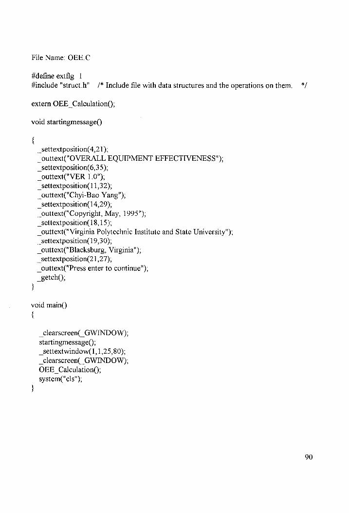
File Name: OEE.C
#define extflg 1 #include "struct.h" /* Include file with data structures and the operations on them.
extern OEE Calculation();
void startingmessage()
{ _settextposition(4,21);
_outtext("OVERALL EQUIPMENT EFFECTIVENESS"); _settextposition(6,35);
_outtext("VER 1.0");
_settextposition(1 1,32);
_outtext("Chyi-Bao Yang");
_settextposition(14,29);
_outtext("Copyright, May, 1995");
_settextposition(18, 15);
_outtext("Virginia Polytechnic Institute and State University"); _settextposition(19,30);
_outtext("Blacksburg, Virginia"); _settextposition(2 1,27);
_outtext("Press enter to continue");
_getch(); }
void main()
{
_clearscreenl GWINDOW); startingmessage();
_settextwindow(1,1,25,80); _clearscreenl_ GWINDOW); OEE Calculation();
system("cls");
*/
90

File Name: OEE _CAL.C
#include "struct.h" /* Include file with data structures and the operations on them. */
extern void EventHandler_start();
extern int get file name();
void Show_Calculation_Form()
{ _settextwindow(1,1,25,80);
_setbkcolor(BLACK);
_settextcolor(WHITE);
_clearscreenl GWINDOW); /* clear the text window by default a 80 x 25 mode) */
_settextposition(1,33);
_outtext("OEE Calculation");
_settextposition(2,33);
_outtext(" ");
_settextposition(3,21);
_outtext("Working Time (min.):");
_settextposition(5,29);
_outtext("Planned Downtime Data" );
_settextposition(6,29);
_outtext(" "):
_settextposition(7,5);
_outtext("Meeting (min.):" );
_settextposition(7,39);
_outtext("Preventive Maintenance (min.):" );
_settextposition(8,5);
_outtext("Break and Holiday (min.):" ); _Settextposition(9,5);
_outtext("Lunch (min.):" );
_Settextposition(9,43);
_outtext("Others (min.):" );
_settextposition(1 1,28);
_outtext("Unplanned Downtime Data" ); _settextposition(12,28);
_outtext(" "). _settextposition(13,5);
_outtext("Setup (min.):" );
_settextposition(13,47);
_outtext("Startup (min.):" );
_settextposition(14,5):;
_outtext("Adjustment (min):" );
91

_Settextposition(14,47),;
_outtext("Minor Stoppage (min.):" );
_settextposition(15,5);
_outtext("Breakdown and Failure (min.):" ); _settextposition(15,47);
_outtext("Idling (min.):" );
_settextposition(16,5);
_outtext("Changeover (min.):" );
_settextposition(16,47);
_outtext("Others (min.):" );
_settextposition(18,33);
_outtext("Process Data" );
_ Settextposition(19,33);
_outtext("——————" ) _settextposition(20, 5);
_outtext("Process Amount (units):" );
_settextposition(20,49);
_outtext("Actual Cycle Time " );
_settextposition(21,5); _outtext("No. of Quality Defect (units):" );
_settextposition(21,45),;
_outtext("(min. per product unit):" );
_Settextposition(22,5);
_outtext("No. of Startup Defect (units):" );
_settextposition(22,49);
_outtext("Design Cycle Time " );
_settextposition(23,5);
_outtext("No. of Rework (units):" );
_settextposition(23,45); _outtext("(min. per product unit):" );
_settextposition(24,4);
_setbkcolor(BLUE);
_settextcolor(RED);
_outtext("CESC: Quit] C*N: New C“L: Load§ C*A: Save As] C“W: "Save{ C*E:
Calculation]");"
j
void Define_Position()
{ Field_Pos[0][0] = 3; Field_Pos[0][1] = 42;
Field Pos[1][0] = 7; Field_Pos[1][1] = 21;
Field_Pos[2][0] = 7; Field_Pos[2][1] = 70;
Field Pos[3]{0] = 8; Field_Pos[3][1] = 31;
92
Field Pos[4][0] = 9; Field_Pos[4][1] = 19;
Field _Pos[5][0] = 9; Field Pos[5][1] = 58;
Field_Pos[6][0] = 13; Field_Pos[6][1] = 19;
Field_Pos[7][0] = 13; Field _Pos[7][1] = 63;
Field_Pos[8][0] = 14; Field_Pos[8][1] = 23;
Field_Pos[9][0] = 14; Field_Pos[9][1] = 70;
Field _Pos[10][0] = 15; Field_Pos[10][1] = 35; Field Pos{11][0] = 15; Field Pos[11][1] = 62;
Field Pos[12][0] = 16; Field Pos[12][1] = 24;
Field_Pos[13][0] = 16; Field_Pos[13][1] = 62;
Field_Pos[14][0] = 20; Field Pos[14][1] = 29;
Field Pos[15][0] = 21; Field_Pos[15][1] = 36; Field_Pos[18][0] = 21; Field Pos[18][1] = 70;
Field Pos[16][0] = 22; Field_Pos[16][1] = 36;
Field_Pos[17][0] = 23; Field _Pos[17][1] = 28;
Field_Pos[19][0] = 23; Field Pos[19][1] = 70;
}
void OEE Calculation()
{
Show_Calculation_Form();
Define_Position();
has_ changed = 1; EventHandler_start(No_Cal_ Fields); return;

File Name: EV HNDLR.C
#include "struct.h"
extern
extern
extern
extern
extern
int quit_from_view(); int get file name); int saveQ);
int print_viewQ);
int clear_data();
void EventHandler_start(No_Cal)
int
{ int
int
int
int
No_Cal;
C, 1, jj length; // Current Field Index
Activate Key_Press; CFNdx;
Activate Key Press = 1; CFNdx = 0;
for (i = 0;i< No_Cal; i++)
{ _settextposition(Field_Pos[i][0], Field_Pos[iJ[1]);
_eprintf("%-9s" Field Value[i]); // display default value
} j= 9; length = 0;
while(Activate_ Key Press)
{ _settextposition((int)Field_Pos[CFNdx][0], (int)Field_Pos[CFNdx][1]+));
if(kbhitQ)) // Check if there is a keypress?
{ c= _getchQ); // Get character without echoing
if (c == Ctrl(‘[')) Activate _Key Press = quit_from_view();
ef (c == Ctrl(‘L')) Activate Key Press = get_file_name(0);
ef (c == Ctrl¢'N’))
{ Activate Key Press = clear_data();
CFNdx = 0;
j= 0; } ef (c == Ctrl('A’)
94

Activate Key Press = get file name(1);
ef (c == Ctrl('W)) Activate Key Press = save();
ef (c == Ctrl(E'))
Activate Key Press = print_viewQ;
ef (c == 8)
{ if (length >= 0)
{ _cputs("");
// Backspace
Field_ Value[CFNdx][}] = (char)32; jj" if Gj > 0)
j--3 length--;
j else
{ _cputs(" "):
BELLQ;
j has_changed = 1;
} ef (c == 75)
{ if (length > 0)
{ ° .
j=j-1, length--;
} else
{ BELLO:
} } ef (c == 77)
{ if (length < 8)
{ 4, length++;
} else
BELLQ;
// Left Arrow
// Right Arrow
//move cursor position
95
} ef (c == 15) // Shift TAB
{ if (CFNdx == 0)
CFNdx = No Cal-1;
else
CFNdx--;
j= 9; length = 0;
} ef ((c == 13) || (c == 9)) // Enter & TAB
{ _settextposition(Field_Pos[CFNdx][0], Field _Pos[CFNdx][1]);
_eprintf("%-9s" Field Value[CFNdx]); // display new value if (CFNdx >= 19)
CFNdx = 0;
else
CFNdx++;
j= 0; length = 0;
} ef ((c >=48 && c <= 57) || (c == 46))
{ if (length < 9)
{ _putch((char)c);
Field_Value[CFNdx][j]=(char)c;
jt; length++;
has_changed = 1; } //move cursor position
else BELLO;
} else
>
} else // Handle other events if no keypress
// You can look for mouse events in this block
96
File Name: CNTLKEY.C
#include "struct.h"
extern void Show Calculation Form();
extern void Define Position();
extern void Calculation; extern void display_results();
extern void _ print_results();
void repaint()
i int 1;
// Clear the text window (by default, a 80x25 one)
Show_Calculation Form();
for (= 0;1< No Cal Fields; 1++)
{ _settextposition(Field_Pos[i][0], Field_Pos[i][1]);
_cprintf("%-9s",Field Value[i]); // display default value
3
}
int clear_data()
t int 1;
i= 0;
for (i= 0;i1< No Cal Fields; i++)
{ strcpy(Field_ Value[i]," ");
} New File = 1;
Show_ Calculation _Form();
Define _Position();
return 1;
}
int Save_As()
{ int i;
OEE File = fopen(filename,"w"); for (i = 0;1< No_Cal_ Fields; i++)
97
fprintf(OEE File,"%9s\n",Field_ Value[i]);
fclose(OEE_ File);
repaint();
has_changed = 0; return 1;
}
int LoadQ)
t int c,i;
if (((OEE File = fopen(filename,"r+"))) = // read_data into Field_ Value
{ _settextposition(1, 1);
_outtext("cannot open "); _outtext(filename);
BELLO;
_settextwindow(10, 10, 15, 70); _setbkcolor(RED);
_settextcolor(WHITE);
_clearscreen@ GWINDOW), _settextposition(S, 1);
_outtext("Press 'y' to create a new or 'n' to exit ");
_settextposition(3, 1);
_outtext("Create a new file? [y/n]:");
_setbkcolor(BLACK),
c=0;
while(1)
{ c=_getch();
if (c =='y' || c =='Y')
{ break;
} if(c == 'n' || c == 'N')
{ repaint();
return 1;
} } New _File = 1;
} else
{ 98
for (i = 0;1< No_Cal_ Fields; i++) fscanf(OEE File,"%9s",Field_Value[i]);
New File = 0;
} fclose(OEE File);
has_changed = 0;
repaint();
return 1;
}
int get file name(Load_or_ Save)
int Load_or_Save;
{ int c, numchar;
_settextwindow(10, 10, 16, 70);
_setbkcolor(RED);
_settextcolor(WHITE);
_clearscreenl GWINDOW);
_settextposition(1, 1); _outtext("Enter OEE filename: "); _settextposition(5, 1);
_outtext("Press <Enter> to continue");
_settextwindow(12, 15, 12, 65);
_setbkcolor(BLACK);
_settextcolor(WHITE);
_clearscreeni GWINDOW),
_settextposition(], 1);
c=0;
numchar = 0;
while(c != ‘\r')
{ c= _getch(;
switch(c)
{ case '\r’: // <Enter>
break;
case \b': // backspace
if(numchar > 0)
{
} break;
filename[--numchar] = '‘\0';
99
default: // all other characters filename[numchar++] = c;
filename[numchar] = ‘\0';
} _clearscreenl@ GWINDOW);
_settextposition(1, 1);
_outtext(filename),
} switch (Load_or_ Save)
{ case 0: return Load(); break;
case 1: return Save As(); _ break; default: break;
} }
int save()
{ int done;
int 1;
if (has_changed)
{ if(New_File)
done = get file name(1);
else
{ OEE File = fopen(filename,"w");
for (1 = 0;1< No Cal Fields; i++)
fprintf(OEE_File,"%9s\n",Field_Value[i]); fclose(OEE File);
j has changed = 0;
j return 1;
}
int quit_from_view()
int Cc;
int return_value; if(has_changed)
100
_settextwindow(10, 10, 15, 70);
_setbkcolor(RED);
_settextcolor(WHITE);
_clearscreenl GWINDOW); _settextposition(5, 1); _outtext("Press 'y' to save file or 'n' to exit without saving file."); _settextposition(3, 1);
_outtext("File changed. Save? [y/n]:");
_setbkcolor(BLACK);
c= 0;
while(1)
{ c=_getch();
== 'y' || c== 'Y')
repaint();
return_value = save();
break;
} if(c == 'n' || c == 'N’) break;
} j return 0;
}
int print_viewQ
{ int c;
_settextwindow(10, 10, 15, 70);
_setbkcolor(RED);
_settextcolor(WHITE);
_clearscreen(@ GWINDOW), _settextposition(5, 1);
_outtext("Press 'y' to do OEE calculation or 'n' to exit "); _settextposition(3, 1);
_outtext("OEE Caluation? [y/n]:");
_setbkcolor(BLACK),
c=0;
while(1)
{ c=_getch();
10]

}
“ == 'y' || == 'Y')
Calculation);
_settextwindow(10, 10, 15, 70);
_setbkcolor(RED); _settextcolor(WHITE);
_clearscreenl@ GWINDOW); _settextposition(5, 1);
_outtext("Press 's' to send results to screen or 'p' to printer "); _settextposition(3, 1); _outtext("Screen or Printer? [s/p]:");
_setbkcolor(BLACK);
c= 0;
while(1)
{ c=_getch();
if(c =='s' || c =='S')
{ display_resultsQ;
break;
} if(c == 'p' || c == 'P')
{ print_resultsQ);
display_resultsQ);
break;
} }
break;
} if(c == 'n' || c == 'N’) break;
} repaint();
return |;
102

File Name: CAL_OPER.C
#include "struct.h"
void display_results()
{ int C;
system("cls"): printf("\n");
printf("\n");
printf¢” Overall Equipment Effectiveness Report"); printf("\n\n"), printf(" Working Time (min.): %9.2f\n", WH);
printf" Planned Downtime (min.): %9.2f\n", PD);
printf(" Loading Time (min.): %9.2f\n", LT);
printf¢" Unplanned Downtime (min.): %9.2f\n", UPD);
printf(" Operating Time (min.): %9.2f\n", OT);
printf("\n\n");
printf(" Number of Good Product (units): %9.2f\n", (float) GP);
printf" Net Operating Rate: %9.2f %%\n", NOR*100);
printf" Operating Speed Rate: %9.2f %%\n", OSR * 100.0);
printf("\n\n");
printf(" Availability: %9.2f %%o\n\n", A*100.0); printfc" Performance Rate: %9.2f %%\n\n", P*100.0);
printf(" Quality Rate: %9.2f %%\n\n", Q*100.0);
printf(" Overall Equipment Effectiveness: %9.2f %%\n\n", OEE*100.0); printf(" Press any key to continue"); c=_getchQ;
}
void CalculationQ)
{
// Calculate Working Time (WH)
WH = (float) atof(Field_Value[0]);
// Caculate Planned Downtimes (PD)
PD = (float)(atof(Field_ Value[1]) + atof(Field_ Value[3]) + atof(Field_ Value[4])
+ atof(Field Value[2]) + atof(Field_ Value[5]));
103

// Calculate Unplanned Downtimes (UPD)
UPD = (float)(atof(Field_ Value[6]) + atof(Field_ Value[8]) + atof(Field_Value[10])
+ atof(Field_ Value[12]) + atof(Field_Value[7]) + atof(Field_ Value[9]) +
atof(Field Value[11]) + atof(Field_ Value[13]));
// Calculate Defect AMount (DA)
DA = (float)(atof(Field_ Value[15]) + atof(Field_ Value[16]) + atof(Field_ Value[17]));
// Calculate Loading TIme (LT)
LT = WH - PD;
// Calculate Operating Time (OT)
OT = LT - UPD;
// Calculate Net Operating Rate (NOR)
NOR = (float)(atof(Field_ Value[14]) * atof(Field_ Value[18]) / OT);
// Calculate Operating Speed Rate (OSR)
OSR = (float)(atof(Field_ Value[19]) / atof(Field_ Value[18]));
// Calculate Number of Good Product
GP = (float) (atof(Field_ Value[14]) - atof(Field_ Value[15]) - atof(Field_ Value[16])
- atof(Field_Value[17]));
// Calculate Availability(A), Performance Rate(P), Quality Rate(Q)
A=OT/LT;
P = NOR * OSR; Q = (float)((atof(Field_ Value[14]) - DA) / atof(Field_ Value[14]));
// Calculate Overall Equipment Effectiveness (OEE)
OEE = A * P *Q; }
104
void print_resultsQ
{ file *fp;
fp = fopen("oee_out.rpt","w");
fprintf(fp, "\n"), fprintf(fp, "\n");
fprintf(fp," Overall Equipment Effectiveness Report");
fprintf(fp,"\n\n"); fprintf(fp, " Working Time (min.): %9.2f\n", WH);
fprintf(fp,” Planned Downtime (min.): %9.2f\n", PD);
fprintf(fp," Loading Time (min.): %9.2f\n", LT); fprintf(fp," Unplanned Downtime (min.): %9.2f\n", UPD);
fprintf(fp," Operating Time (min.): %9.2f\n", OT);
fprintf(fp, "\n\n"),
fprintf(fp," Number of Good Product (units): %9.2f\n", (float) GP);
fprintf(fp," Net Operating Rate: %9.2f %%\n", NOR*100);
fprintf(fp," Operating Speed Rate: %9.2f %%\n", OSR * 100.0);
fprintf(fp, "\n\n");
fprintf(fp," Availability: %9.2f %%o\n\n", A*100.0); fprintf(fp," Performance Rate: %9.2f %%\n\n", P*100.0);
fprintf(fp," Quality Rate: %9.2f %%\n\n", Q* 100.0);
fprintf(fp,” Overall Equipment Effectiveness: %9.2f %%\n\n", OEE*100.0);
fclose(fp);
system("cls");
system("print oee_out.rpt");
105
File Name: STRUCT.H
#include <stdio.h> /* input output utilities */
#include <string.h> /* string declaration */ #include <time.h> /* time-conversion routines */
#include <math.h> /* math functions */
#include <stdlib.h> /* memory allocation */
#include <process.h> /* system functions */
#include <graph.h> /* text window functions */ #include <conio.h> /* console I/O functions */
#ifndef extflg
# define extdef extern
#else
# define extdef
#Hendif
#ifndef TRUE /* If TRUE has not been defined, TRUE = 1 */
#define TRUE 1
#endif
#ifndef FALSE /* If FALSE has not been defined, then FALSE = 0 */
#define FALSE 0
#endif
#define BLACK
#define BLUE
#define GREEN
#define CYAN
#define RED
#define MAGENTA
#define BROWN
#define WHITE
#define GRAY
#define LIGHTBLUE
#define LIGHTGREEN
#define LIGHTCYAN
#define LIGHTRED
#define LIGHTMAGENTA
#define YELLOW
#define BRIGHTWHITE
#define Ctrl(X) (X-0x40)
OoOo
nD
A ABW
N & ©
Ree
eS eae
eS
SS IO
Cn BW
NO
—] ©
/* control character */
106
#define ef else if
#define BELLQ _putch((char)7)
#define No_Cal_Fields20 extdef int
extdef char
extdef int
extdef int
extdef FILE
extdef char
Field_Pos[20][2];
Field_Value[20][9];
has_changed;
New _File;
*OEE File;
filename[80];
// Calculation Variables
extdef float
extdef float
extdef float
extdef float
extdef float
extdef float
extdef float
extdef float
extdef float
extdef float extdef float
extdef float
extdef float
extdef float
extdef float
WH; PD;
UPD;
DA: 9
/* Bell sound */
107

jepow FAO
pazuaindwod jo
uses9g ynduy
‘| -y sund14
lkuorqetnote9 :q_{|
lfeaes :m_j|
lfsw anes
:w_{| lHpeod
:4_4| lfmen
en dl
ly tnG :osall
G°O
:(3tuN
YOnpoid
azed -utw)
Oo :(s3ztun)
yYIOMBsY FO
"ON QUT L
9@[TOAD ubtseg
0 :(S3tTUN)
YZazZaq
dnyzeys
Jo °ON
8°O :(4tun
yoOnpoad
asd
-utw)
g :(sqztun)
Zoazaq
AATTeNG
Jo °ON
BUTI
@TOAD
Ten oy
OOP
:(Ss}ztuN)
JUNOUWYW
SsS2eD01g
e\yeg sseD01g
QO :(*°utw)
SzayAO
Oo :(*utw)
reacabueyy)
O :("utw)
BbutTpr
Of :(*utu)
sin~Tteq
pue
umoOpyesig
QO :(*‘utw)
abeddoqys
z0uTtW OZ
:(utw)
jusuqysn(py
Oo :(*utTw)
dnqizeq4s Oz
:(*utw)
dnjas
ejeg
suT\UMOG
pouUeTduy
O :(*utw) siay IO
QO :(*°utw)
youny
Oo :(°utw)
AeptTOH
pue
yeaig
OZ :(‘utw)
sdueUs,UTeW
BATRUBAZId
0 :(°utu)
ButAseyp
e}eg
|aUT}UMOG
peuUeTd
O8p :(*uTWw)
suTy
ButyrI0Mm
UOT}FETNITeD FAO
108

Overall Equipment Effectiveness Report
Working Time (min. ): 480.00
Planned Downtime (min. ): 20.00
Loading Time (min. ): 460.00
Unplanned Downtime (min. ): 60.00
Operating Time (min.): 400.00
Number of Good Product (units): 392.00
Net Operating Rate: 80.00 % Operating Speed Rate: 62.50 %
Availability: 86.96%
Performance Rate: 50.00%
Quality Rate: 98 00%
Overall Equipment Effectiveness: A? 61% Figure A.2 Output of Computerized OEE model
109