PPC Course new

8/4/2019 PPC Course new

http://slidepdf.com/reader/full/ppc-course-new 1/83

ForecastingPPC Course 2

Industrial Engineering Department

Sepuluh Nopember Institute of Technology

Indonesia 2008



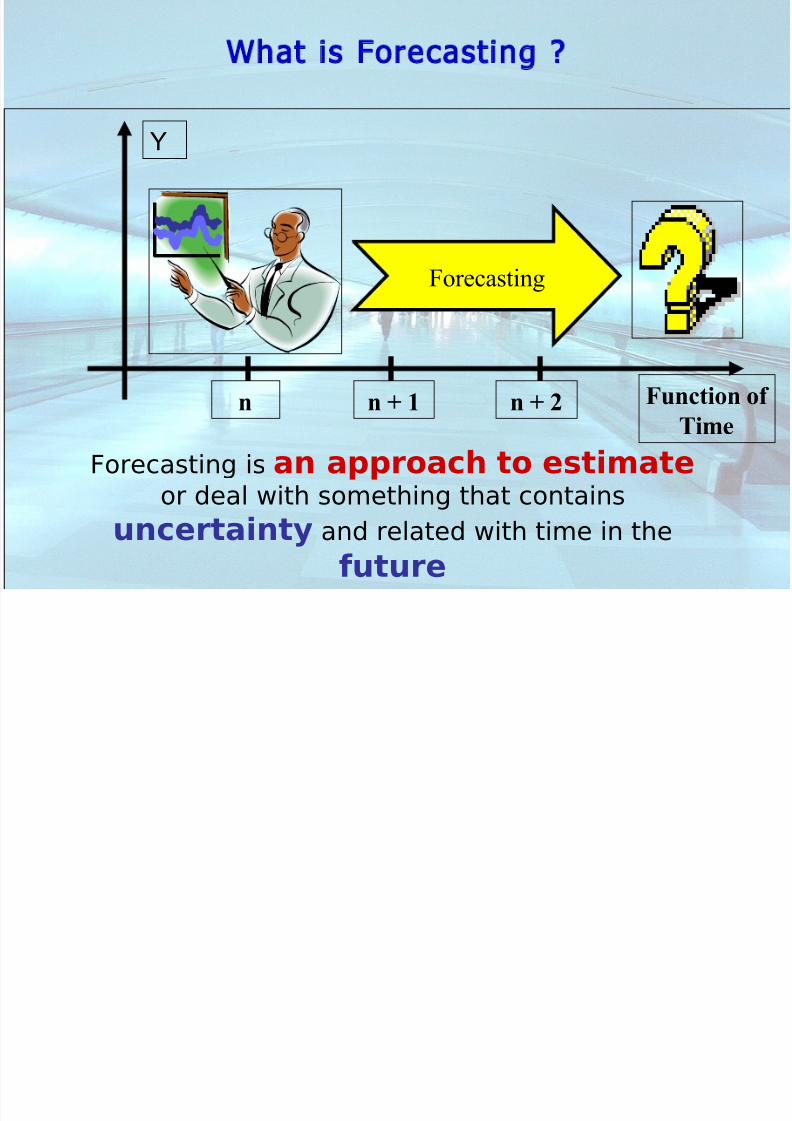
What is Forecasting ?

Forecasting

Y

n n + 1 n + 2Function of

Time

Forecasting is an approach to estimate

or deal with something that contains

uncertainty and related with time in the

future



What is forecasting ?

• The process of estimating future demand in terms of thequantity, timing, quality, and location for desired productsand services

• Rely on logical methods of manipulating data that havebeen generated by historical events

• Forecasting is an essential element of capital budgeting.

Sales will be$200 Million!



why we need forecasting?

• All organizations operate in an atmosphere of uncertainty and become more complex

• All decisions must be made for uncertainty

future based on imperfect knowledge• Educated guesses more valuable than

uneducated guesses

• Not to say that intuitive forecasting is bad• The quantitative forecasting technique to bethe starting point in the effective forecastingand valuable supplement



Who needs forecasts?

• Every organization, large and small, privateand public, must plan to meet the condition of the future for which it has imperfectknowledge.

• Across all functional line: finance, marketing,personnel, and production areas.



Characteristics of forecasting

• Forecasts are usually wrong, seldom correct, andinvolves error find the best method

• Forecast should include a measure of forecast

error• Forecasting methods assume there is some

underlying stability in the system• Family / grouped / aggregated data forecasts

are usually more accurate than item forecast• Short range forecasts are more accurate than

long-range forecast



Forecasting in Business

• Marketing - sale forecast

• Operations - capacity, scheduling,

inventory



Assumptions of Forecast

• Information (data) about the past is

available

• The pattern of the past will continue into thefuture (Time Series Models).



Forecast in MTO

•Forecast tidak banyak dikenal dan dipergunakan diperusahaan Make To Order

• Overproduction di perusahaan dengankarakteristik MTO justru adalah kerugian

• Forecast bukan merupakan isu utama di MTO, justru isu utama adalah nervousness system,responsiveness, dan material management (Pujawan, 2000).

• Pada MTO, forecast tidak lagi dilakukan terhadapdemand, melainkan pada penggunaan resource dimasa datang.

But, demand forecast is very useful in MTS



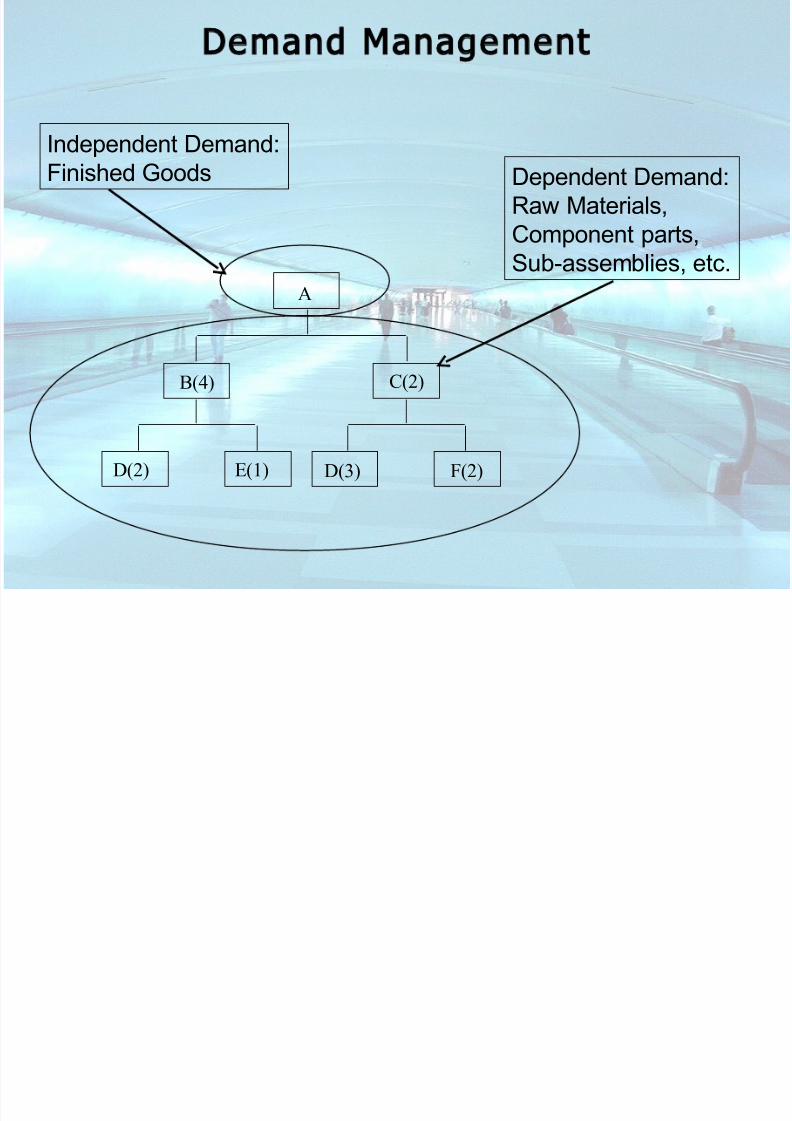
Demand Management

A

B(4) C(2)

D(2) E(1) D(3) F(2)

Dependent Demand:

Raw Materials,

Component parts,

Sub-assemblies, etc.

Independent Demand:Finished Goods



Forecasting Steps

• Decide what needs to be forecast – Level of detail, units of analysis & time horizonrequired

• Evaluate and analyze appropriate data

– Identify needed data & whether it’s available• Select and test the forecasting model – Cost, ease of use & accuracy

• Generate the forecast

• Monitor forecast accuracy over time



Characteristics of a good forecast

• Accuracy bias (when forecast arepersistently too high or too low) & consistency (concerned with the size of forecast error)

• Cost

• Response stability & responsive

• Simplicity easy to make, understand & use



Types of Forecasting Methods

Depend on : – TIME FRAME

Indicates how far into the future is forecast

• Short- to mid-range forecast – typically encompasses the immediate future

– daily up to two years• Long-range forecast

– usually encompasses a period of time longer than twoyears

– DEMAND BEHAVIOR

– CAUSES OF BEHAVIOR



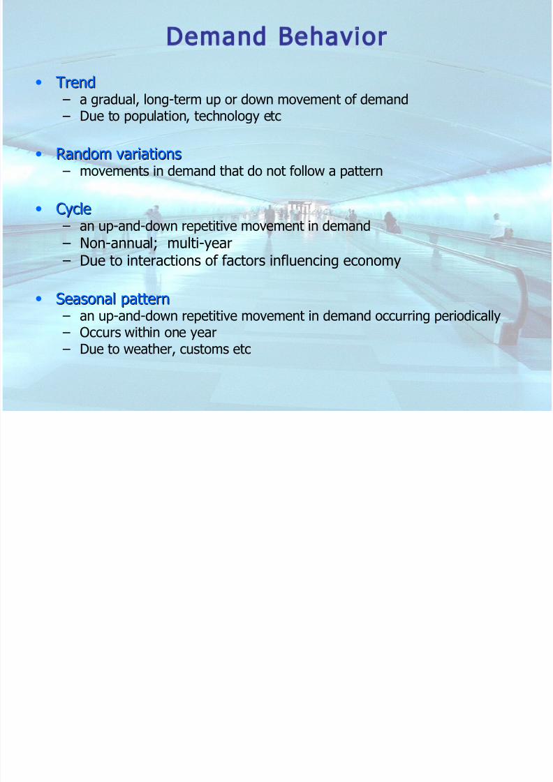
Demand Behavior

• TrendTrend

– a gradual, long-term up or down movement of demand – Due to population, technology etc

• Random variationsRandom variations – movements in demand that do not follow a pattern

• CycleCycle – an up-and-down repetitive movement in demand – Non-annual; multi-year – Due to interactions of factors influencing economy

• Seasonal patternSeasonal pattern – an up-and-down repetitive movement in demand occurring periodically – Occurs within one year – Due to weather, customs etc



TimeTime(a) Trend(a) Trend

TimeTime(d) Trend with seasonal pattern(d) Trend with seasonal pattern

TimeTime(c) Seasonal pattern(c) Seasonal pattern

TimeTime(b) Cycle(b) Cycle

D e m a n d

D e m a n d

D e m a n

d

D e m a n d

D e m a n d

D e m a n d

D e m a n d

D e m a n d

RandomRandommovementmovement

Forms of Forecast Movement



Components of an Observation

Observed demand (O) =

Systematic component (S) + Random component(R)

Level (current deseasonalized demand)

Trend (growth or decline in demand)

Seasonality (predictable seasonal fluctuation)

• Systematic component: Expected value of demand• Random component: The part of the forecast that deviates

from the systematic component• Forecast error: difference between forecast and actual demand

Chopra, 2007



Forecasting Process (in general)

6. Check forecast

accuracy with one or

more measures

4. Select a forecast

model that seems

appropriate for data

5. Develop/compute

forecast for period of

historical data

8a. Forecast over

planning horizon

9. Adjust forecast based

on additional qualitative

information and insight

10. Monitor results

and measure forecast

accuracy

8b. Select new

forecast model or

adjust parameters of

existing model

7.

Is accuracy of

forecast

acceptable?

1. Identify the

purpose of forecast

3. Plot data and identify

patterns

2. Collect historical data

No

Yes

Copyright 2006 John Wiley & Sons, Inc.Copyright 2006 John Wiley & Sons, Inc.



Forecasting Technique

Forecasting

Models

Qualitative Quantitative

CausalTime serie

Regression EconometricMoving

average DecompositionExponential

smoothing

Sales forc

composite

Consume

survey

Jury of

executiv

Delphi

method

ARIMA Neural

networks



Forecasting

• Predicting the Future

• Qualitative forecast methods

– Subjective (uses experience

and judgment to establishfuture behaviours)

• Quantitative forecast methods

– based on mathematicalformulas

– uses historical data toestablish relationships andtrends which can beprojected into the future



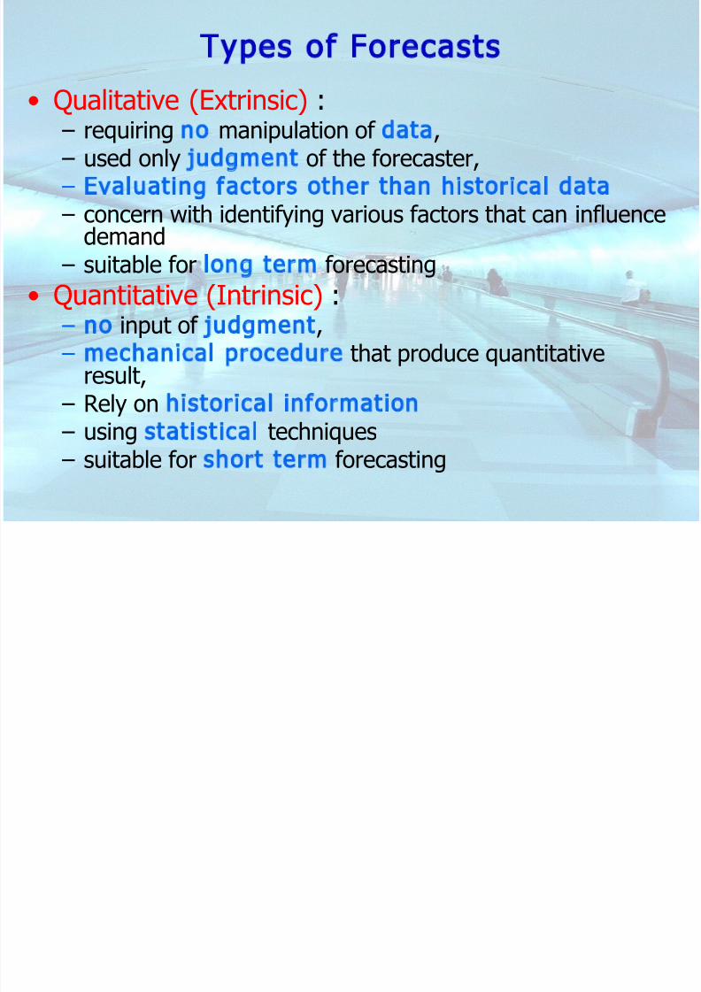
Types of Forecasts

• Qualitative (Extrinsic) : – requiring no manipulation of data, – used only judgment of the forecaster, – Evaluating factors other than historical data – concern with identifying various factors that can influence

demand – suitable for long term forecasting

• Quantitative (Intrinsic) : – no input of judgment, – mechanical procedure that produce quantitative

result, – Rely on historical information – using statistical techniques – suitable for short term forecasting



• Causal• Judgment

• Causal• Judgment

• Time series• Causal• Judgment

ForecastingTechnique

• Facil ity location• Capacityplanning

• Processmanagement

• Staff planning• Productionplanning

• Master productionscheduling

• Purchasing• Distribution

• Inventorymanagement

• Final assemblyscheduling

• Workforce

scheduling• Master productionscheduling

Decision

Area

• Total salesTotal sales• Groups or families

of products or

services

• Individual

products orservices

ForecastQuality

Long Term(more than 2 years)

Medium Term(3 months– 2

years)

Short Term

(0–3 months)

Application

Time Horizon

Demand Forecast Applications



Detail steps inchoosing

forecast method



The keys to employing qualitative forecasting are:

• Data as an historicalseries is notavailable,or is not

relevant to futureneeds.

♦An unusual product or a

unique project is being

contemplated.

1. Qualitative Methods (Extrinsic)



1. Qualitative Methods (Extrinsic)

• Applications: New product Development,new technology

• Technique : – Management Decision – Jury of executive opinion

– Delphi Technique – Sales Force Composite – Growth curve – Scenario writing

– Market Research – Historical Analogies – Life Cycle Curves – Focus groups



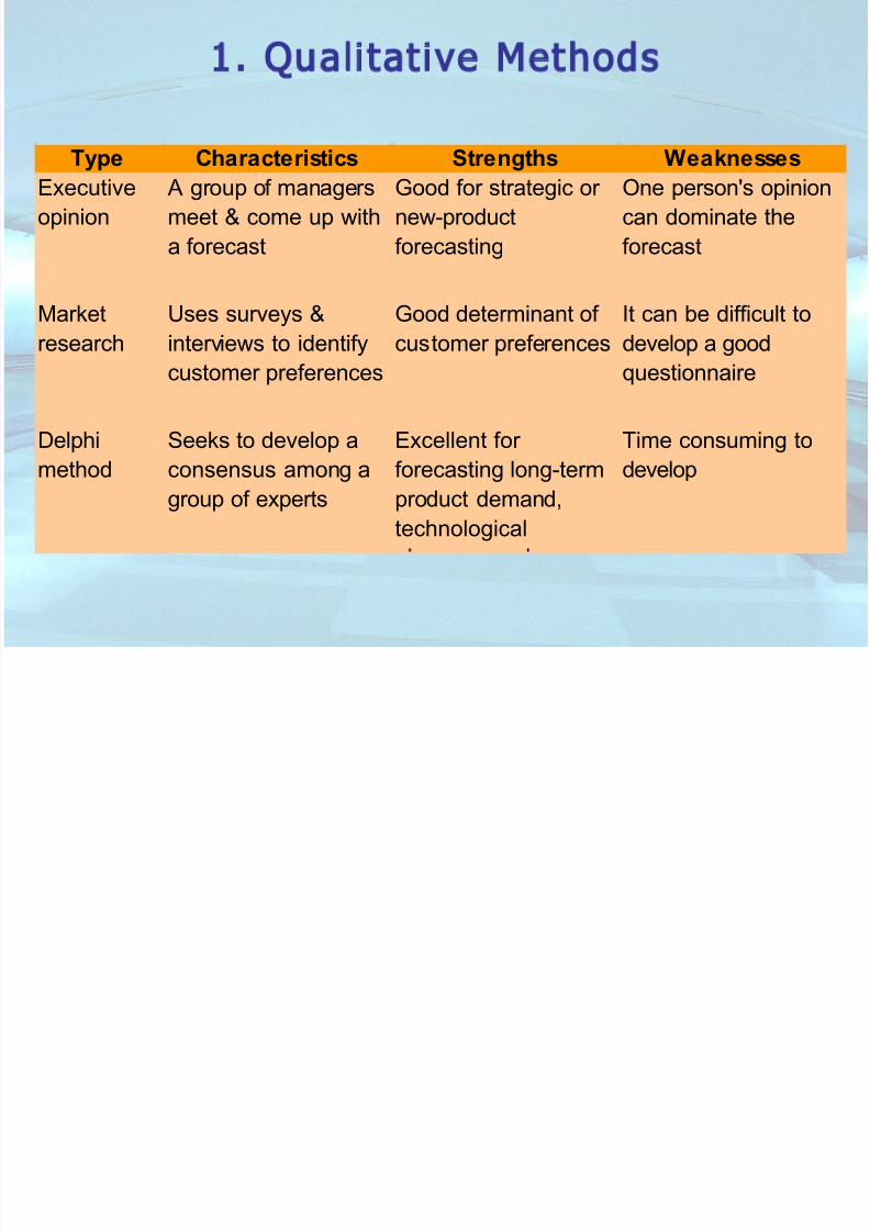
1. Qualitative Methods

Type Characteristics Strengths WeaknessesExecutive

opinion

A group of managers

meet & come up with

a forecast

Good for strategic or

new-product

forecasting

One person's opinion

can dominate the

forecast

Market

research

Uses surveys &

interviews to identify

customer preferences

Good determinant of

customer preferences

It can be difficult to

develop a good

questionnaire

Delphi

method

Seeks to develop a

consensus among a

group of experts

Excellent for

forecasting long-term

product demand,

technological

Time consuming to

develop



1. Qualitative Methods- in g e ne r a l -i n g ene r a l -

Kelebihan :– Mampu melakukan

prediksi walaupuntidak ada dukungan

data historis– Umumnya cukup valid

karena melibatkanpara expert yang

kompeten denganpermasalahan yangterjadi, sehinggamodel dan metodeyang dipergunakancukup akurat

Kelemahan :

– Cost – nya sangattinggi karenamelibatkan expert terkait denganlabour time

– Memakan waktuyang cenderunglama apalagi

“Building Models &Methods”memerlukanvalidasi guna hasil

yang relevan



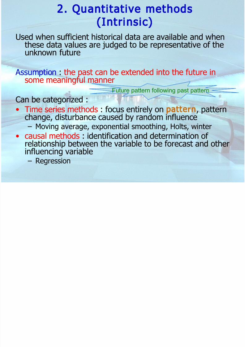
2. Quantitative methods(Intrinsic)

Used when sufficient historical data are available and when

these data values are judged to be representative of theunknown future

Assumption : the past can be extended into the future insome meaningful manner

Can be categorized :• Time series methods : focus entirely on pattern, pattern

change, disturbance caused by random influence

– Moving average, exponential smoothing, Holts, winter• causal methods : identification and determination of relationship between the variable to be forecast and otherinfluencing variable – Regression

Future pattern following past pattern



2.1 Time series methods

Time series consist of data that are collected /observed over successive increment of time

Assumption : What happen in the past willcontinued and occurs in the future with special

pattern followed.Exploring the data pattern

• Display data → time series graph

• Autocorrelation test • Understanding what the data are suggesting

Future pattern following past pattern



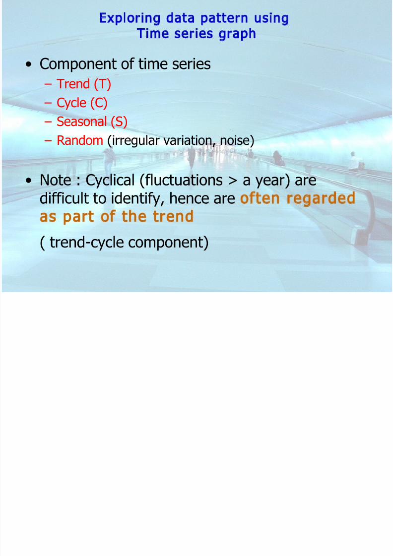
Exploring data pattern usingTime series graph

• Component of time series – Trend (T)

– Cycle (C)

– Seasonal (S)

– Random (irregular variation, noise)

• Note : Cyclical (fluctuations > a year) aredifficult to identify, hence are often regardedas part of the trend

( trend-cycle component)



Types of Time Series Models

• Nonseasonal Model

– Trend, Naïve – Moving average – Weighted moving average – Exponential Smoothing

• Seasonal Model

– Time Series Decomposition – ARIMA – Artificial Neural Network (ANN)

• Seasonal & Trend

– Winter

(Trend & Seasonality CorrectedExponential Smoothing)

• Trend Model

– Holt’s Model

(Trend corrected Exponential Smoothing)

Moving Average Model

Capture Trend & Seasonal

Exponential Smoothing Model Trend and sometimes Seasonal(Holt and Winter Model)

Decomposition Almost all, except Cycle (Candecompose but the value for recompose need judgment fromthe user)

Not discussed



Trend Model

• Trend Model sangat tepat dipergunakan apabila karakteristik data cenderung jelas

bersifat trend.• Prinsip Trend adalah mencoba melakukan Curve Fitting berdasarkan suatu model

persamaan tertentu untuk mendapatkan persamaan garis yang merefleksikan kondisidata aktual dengan menjadikan nilai t (waktu) sebagai variabel independen

• Beberapa model persamaan garis yang dipergunakan : – Linear Simple Linear Regression sebagai fungsi t y = ax + b + e

– Kuadratik Y t = a + bt + ct 2

– Power Y t = at b

– Model persamaan garis lainnya S – Curve, Eksponential, dll

0

0

0

0

0

0

0

0

0 0 0 0 0 0 0 0 0 00

0

000

0000

0000

0000

0000

0000

0 0 0 0 0 0 0 0 0 00

Power

Quadratic



Application of Trend using Software

Using Minitab

• Minitab pada perhitungan Trendmempergunakan 4 persamaangaris

– Linear

– Kuadratik

– Eksponential – S – Curve

• Klik Analyze Time Series Trend Analysis

SPPS 10.0 for Windows• SPSS menggunakan 11 Persamaangaris, yaitu

– Linear - Logaritma

– Inverse - Kuadratik

– Kubik - Power – Compound - S – Curve

– Logistics - Growth

– Eksponential

• Klik Analyze

Regression

CurveEstimation

MINITAB.lnk



EXAMPLE – (Trend Projection)

Periods Sales

January 185

February 174

March 200

April 210May 205

June 245

July 234

August 250

September 264

October 245

November 235

December 242

PT Makmur Jaya mempunyai data sales selama 2003

sebagaimana data disamping. Anda sebagai Planner

perusahaan ditugaskan untuk membuat estimasi sales Januari

– Februari 2004. Berdasarkan hasil plotting, anda melihat

kecenderungan data yang menaik tanpa adanya efek seasonal,

sehingga anda memutuskan akan menggunakan trend

projection, dengan 4 pers. Garis, linear, kuadratik, power, dan

kubik. Setelah diperhitungkan, mana yang akan anda pilihsebagai rumusan anda ???

Sales

000111

000 000 000

000111

000 111000 000 000

0

00

000

000

000

000

000

J a n u

a r

F e b r

u a r

M a r c h

A p r i l

M a y

J u n e

J u l y

A u g u

s

S e p t e m b

O c t o b e

N o v e

m b e

D e c e m b e

Moths

S a l e



EXAMPLE (Trend Projection) – Cont’d

Power Kubik Kuadratik Linear HistoryError Powe Fit Powe Error Cubic Fit Cubic Error Kuadrat Fit Kuadrat Error Linear Fit Linear Sales Periods

184,00 1,00 93,85 91,15 121,56 63,44 156,66 28,34 185 January

178,26 6,74 27,36 157,64 66,52 118,48 128,32 56,68 174 February

164,40 20,60 18,07 203,07 19,88 165,12 99,98 85,02 200 March

139,51 45,49 46,01 231,01 18,37 203,37 71,64 113,36 210 April

100,90 84,10 60,06 245,06 48,22 233,22 43,30 141,70 205 May

46,05 138,95 63,80 248,80 69,68 254,68 14,96 170,04 245 June

27,43 212,43 60,83 245,83 82,74 267,74 13,38 198,38 234 July

121,83 306,83 54,72 239,72 87,40 272,40 41,72 226,72 250 August

239,39 424,39 49,08 234,08 83,66 268,66 70,06 255,06 264 SEPT.

382,25 567,25 47,48 232,48 71,53 256,53 98,40 283,40 245 October

552,49 737,49 53,52 238,52 51,00 236,00 126,74 311,74 235 NOV

752,17 937,17 70,78 255,78 22,08 207,08 155,08 340,08 242 DECEM

240,72 53,80 61,89 85,02 MAD

101204,41 3242,43 4733,66 9571,56 MSD



Moving Average

• Na i v e forecast – demand the current period is used as nextperiod’s forecast

• Simple moving average

– stable demand with no pronounced behavioralpatterns

• Weighted moving average

– weights are assigned to most recent data



Moving Average:Naïve Approach

JanJan 120120

FebFeb 9090Mar Mar 100100

Apr Apr 7575

MayMay 110110

JuneJune 5050

JulyJuly 7575

AugAug 130130

SeptSept 110110

OctOct 9090

ORDERSORDERS

MONTHMONTH PER MONTHPER MONTH

--

1201209090

100100

7575

110110

5050

7575

130130

110110

9090Nov -Nov -

FORECASTFORECAST



Simple Moving Average

MAMAnn ==

nn

i i = 1= 1 DDi i

nn

wherewhere

nn == number of periodsnumber of periods

in the movingin the moving

averageaverageDDi i == demand in perioddemand in period i i

3 month Simple Moving3 month Simple Moving



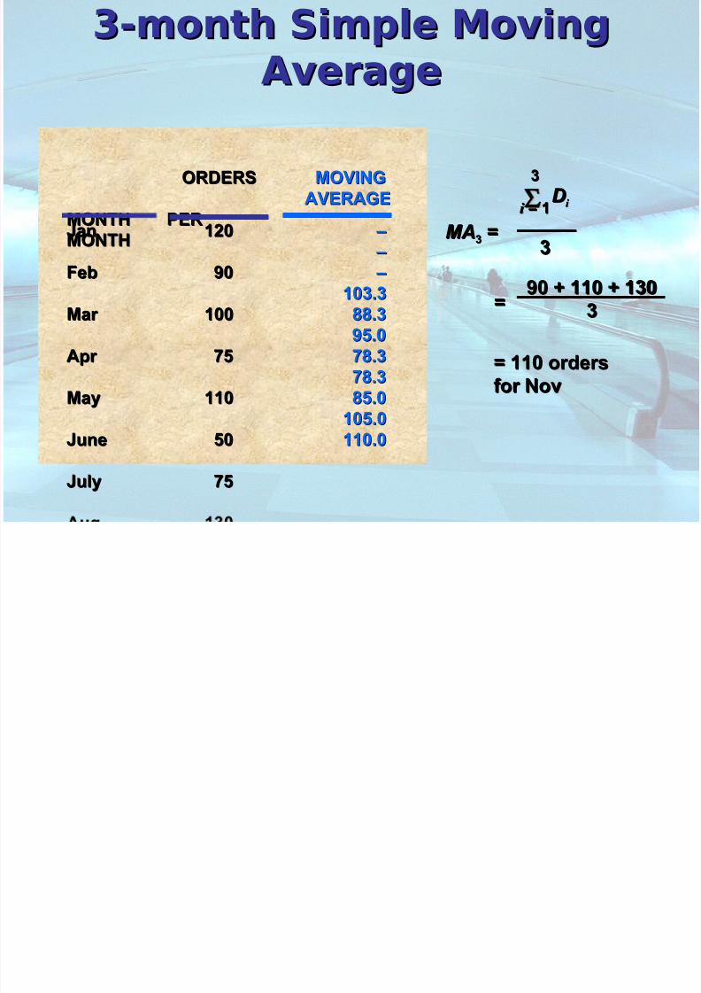
3-month Simple Moving3-month Simple Moving

AverageAverage

JanJan 120120

FebFeb 9090

Mar Mar 100100

Apr Apr 7575

MayMay 110110

JuneJune 5050

JulyJuly 7575

ORDERSORDERS

MONTHMONTH PERPER

MONTHMONTH MAMA33 ==

33

i i = 1= 1DDi i

33

==90 + 110 + 13090 + 110 + 130

33

= 110 orders= 110 ordersfor Novfor Nov

– –

– – – –

103.3103.3

88.388.3

95.095.0

78.378.3

78.378.385.085.0

105.0105.0

110.0110.0

MOVINGMOVING

AVERAGEAVERAGE

5 month Simple Mo ing



5-month Simple MovingAverage

JanJan 120120

FebFeb 9090

Mar Mar 100100

Apr Apr 7575

MayMay 110110

JuneJune 5050

JulyJuly 7575

AugAug 130130

ORDERSORDERS

MONTHMONTH PERPER

MONTHMONTH MAMA5 5 ==

55

i i = 1= 1DDi i

55

==90 + 110 + 130+75+5090 + 110 + 130+75+50

55

= 91 orders= 91 orders

for Novfor Nov

– –

– –

– – – –

– –

99.099.0

85.085.0

82.082.0

88.088.0

95.095.0

91.091.0

MOVINGMOVING

AVERAGEAVERAGE



Smoothing Effects

150150 –

125125 –

100100 –

7575 –

5050 –

2525 –

00 –

| | | | | | | | | | |

JanJan FebFeb Mar Mar Apr Apr MayMay JuneJune JulyJuly AugAug SeptSept OctOct NovNov

ActualActual

O r d e r s

O r d e r s

MonthMonth

5-month5-month

3-month3-month



Weighted Moving Average

WMAWMAnn ==

i i = 1= 1Σ W W

i i DDi i

wherewhere

W W i i = the weight for period= the weight for period i i ,,

between 0 and 100between 0 and 100

percentpercent

Σ W W i i = 1.00= 1.00

Adjusts Adjusts

movingmoving

averageaveragemethod tomethod to

more closelymore closely

reflect datareflect datafluctuationsfluctuations



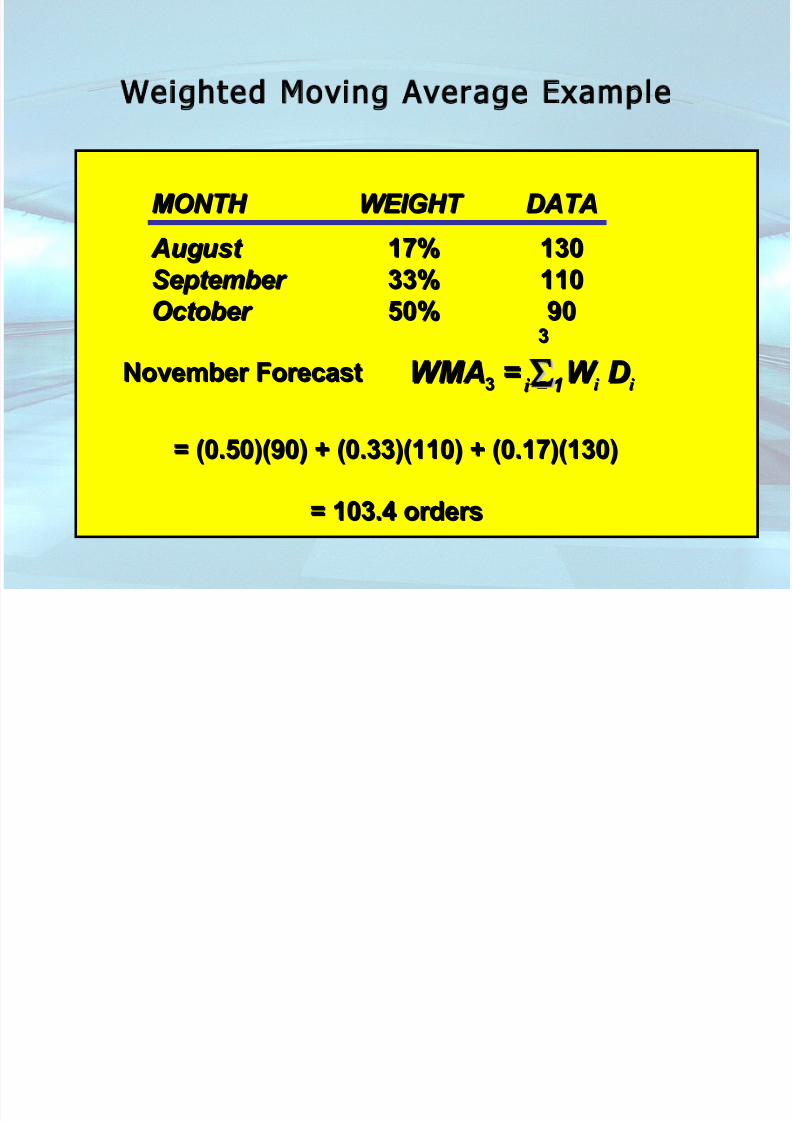
Weighted Moving Average Example

MONTH MONTH WEIGHT WEIGHT DATADATA

August August 17%17% 130130

September September 33%33% 110110October October 50%50% 9090

WMAWMA33 ==

33

i i = 1= 1 W W i i DDi i

= (0.50)(90) + (0.33)(110) + (0.17)(130)= (0.50)(90) + (0.33)(110) + (0.17)(130)

= 103.4 orders= 103.4 orders

November ForecastNovember Forecast



• Increasing n makesforecast less sensitive to

changes• Do not forecast trends well

• Require sufficient historicaldata

Disadvantages of M.A. Methods



Averaging method Averaging method

Weights most recent data more stronglyWeights most recent data more strongly

Reacts more to recent changesReacts more to recent changes

Widely used, accurate methodWidely used, accurate method

Exponential Smoothing



Exponential Smoothing: Notation

• Level of the time series at time t :• Trend in the time series at time t :

• Seasonal index in the the time series

at time t :• Level smoothing parameter:

• Trend smoothing parameter:

• Seasonal index smoothing parameter:

• Number of seasons: M

t

L

t T

t S

00 ≤≤α

00 ≤≤ β

00 ≤≤ γ



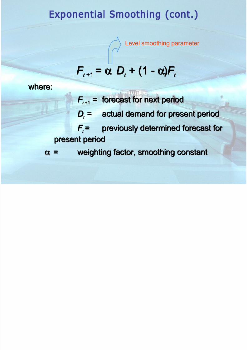
F F t t +1+1 == αα DD

t t + (1 -+ (1 - αα))F F

t t

where:where:F F

t t +1+1 == forecast for next periodforecast for next period

DDt t == actual demand for present periodactual demand for present period

F F t t == previously determined forecast for previously determined forecast for present periodpresent period

αα == weighting factor, smoothing constantweighting factor, smoothing constant

Exponential Smoothing (cont.)

Level smoothing parameter



Effect of Smoothing Constant

0.00.0 ≤ α ≤≤ α ≤ 1.01.0

If If αα = 0.20, then= 0.20, then F F t t +1+1 = 0.20= 0.20 DDt t + 0.80+ 0.80 F F t t

If If αα = 0, then= 0, then F F t t +1+1 = 0= 0 DD

t t + 1+ 1 F F

t t 0 =0 = F F t t

Forecast does not reflect recent dataForecast does not reflect recent data

If If αα = 1, then= 1, then F F t t +1+1 = 1= 1 DD

t t + 0+ 0 F F

t t == DDt t

Forecast based only on most recent dataForecast based only on most recent data

F F t t +1+1 == α DDt t + (1 -+ (1 - α))F F t t



F F 22 == αDD11 + (1 -+ (1 - α))F F 11

= (0.30)(37) + (0.70)(37)= (0.30)(37) + (0.70)(37)

= 37= 37

F F 33 == αDD22 + (1 -+ (1 - α))F F 22

= (0.30)(40) + (0.70)(37)= (0.30)(40) + (0.70)(37)

= 37.9= 37.9

F F 1313 == αDD1212 + (1 -+ (1 - α))F F 1212

= (0.30)(54) + (0.70)(50.84)= (0.30)(54) + (0.70)(50.84)

= 51.79= 51.79

Exponential Smoothing (α=0.30)

PERIODPERIOD MONTHMONTH

DEMANDDEMAND

11 JanJan 3737

22 FebFeb 4040

33 Mar Mar 4141

44 Apr Apr 3737

55 MayMay 4545

66 JunJun 5050

77 JulJul 4343

F F t t +1+1 == α DDt t + (1 -+ (1 - α))F F t t



FORECAST,FORECAST, F F t t + 1+ 1

PERIODPERIOD MONTHMONTH DEMANDDEMAND ((α = 0.3)= 0.3) ((α = 0.5)= 0.5)

11 JanJan 3737 – – – –

22 FebFeb 4040 37.0037.00 37.0037.00

33 Mar Mar 4141 37.9037.90 38.5038.50

44 Apr Apr 3737 38.8338.83 39.7539.75

55 MayMay 4545 38.2838.28 38.3738.37

66 JunJun 5050 40.2940.29 41.6841.68

77 JulJul 4343 43.2043.20 45.8445.84

88 AugAug 4747 43.1443.14 44.4244.42

99 SepSep 5656 44.3044.30 45.7145.71

1010 OctOct 5252 47.8147.81 50.8550.851111 NovNov 5555 49.0649.06 51.4251.42

1212 DecDec 5454 50.8450.84 53.2153.21

1313 JanJan – – 51.7951.79 53.6153.61




7070 –

6060 –

5050 –

4040 –

3030 –

2020 –

1010 –

00 –

| | | | | | | | | | | | |

11 22 33 44 55 66 77 88 99 1010 1111 1212 1313

ActualActual

O r d e r s

O r d e r s

MonthMonth


α = 0.50= 0.50

α = 0.30= 0.30

Larger α, more responsive forecast;

Smaller α, smoother forecast

“Best” α can be found by Solver Suitable for relatively stable time

series



Simple Exponential Smoothing

• A special type of weighted moving average – Include all past observations – Use a unique set of weights that weight recent observations

much more heavily than very old observations

α

α α

α α

α α

( )

( )

( )

0

0

0

0

0

−

−

−

weightDecreasing weightsgiven

to olderobservations

0 0< <α

Toda

Compa ison of E ponential Smoothing and Simple



Comparison of Exponential Smoothing and SimpleMoving Average

• Both Methods – Are designed for stationary demand – Require a single parameter – Lag behind a trend, if one exists

– Have the same distribution of forecast error if

• Moving average uses only the last N periods data,exponential smoothing uses all data

• Exponential smoothing uses less memory and requiresfewer steps of computation; store only the most recentforecast!

)0/(0 +=α N



Trend-Corrected ExponentialSmoothing (Holt ’s Model)

• Appropriate when the demand is assumed to have alevel and trend in the systematic component of demand but no seasonality

• Obtain initial estimate of level and trend by running a

linear regression of the following form:D t = at + b

T0 = a

L0 = b

In period t, the forecast for future periods isexpressed as follows:Ft+1 = Lt + Tt

Ft+n = Lt + nTt

Demand & time

correlation is linear



Trend-Corrected ExponentialSmoothing (Holt ’s Model)

After observing demand for period t, revise theestimates for level and trend as follows:Lt+1 = αDt+1 + (1-α)(Lt + Tt)

Tt+1 = β(Lt+1 - Lt) + (1-β)Tt

α = smoothing constant for levelβ = smoothing constant for trendExample 7.3, p. 188: Tahoe Salt demand data.

Forecast demand for period 1 using Holt’s model

(trend corrected exponential smoothing)Using linear regression,L0 = 12015 (linear intercept)

T0 = 1549 (linear slope)



Quarter Demand Dt

II, 0000 1111

III, 0000 11111

IV, 0000 00000

I, 0000 11111

II, 0000 00000

III, 0000 00000

IV, 0000 00000

I, 0000 00000

II, 0000 00000III, 0000 00000

IV, 0000 00000

I, 0000 00000

Quarterly Demand for Tahoe SaltTable 7.1 (Chopra, p. 180)

Forecast demand

for the next four

quarters.



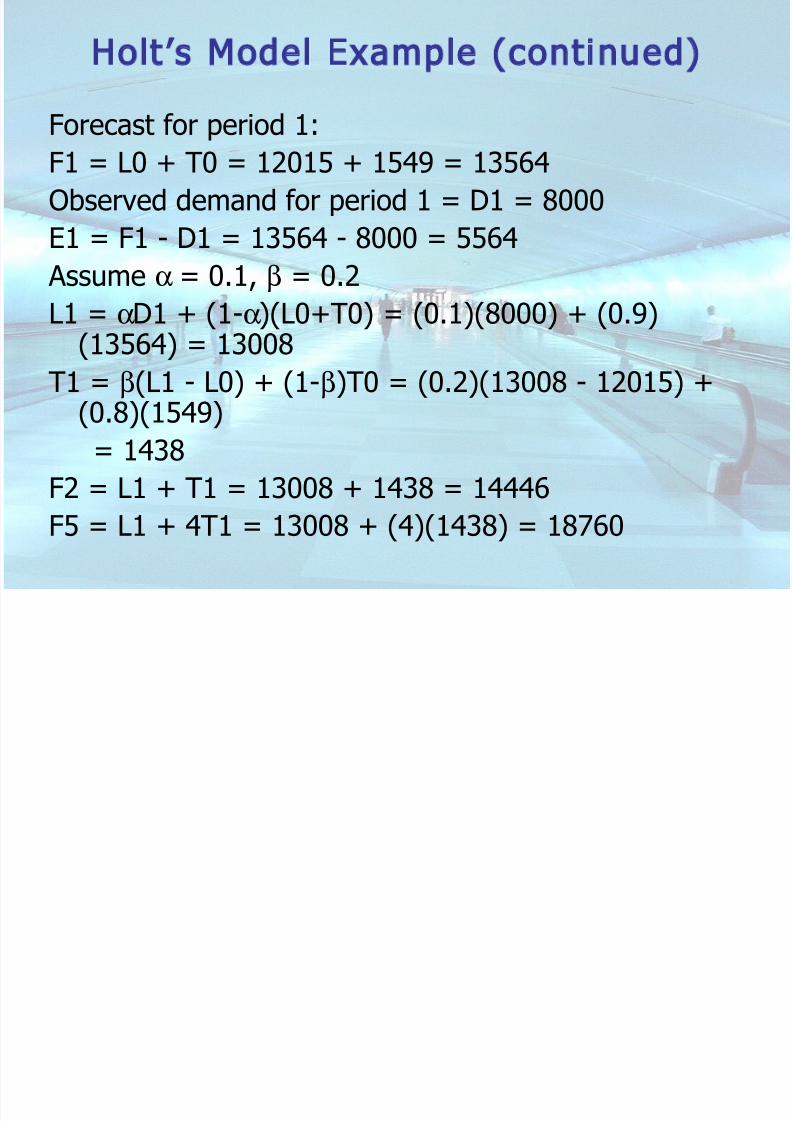
Holt’s Model Example (continued)

Forecast for period 1:F1 = L0 + T0 = 12015 + 1549 = 13564Observed demand for period 1 = D1 = 8000E1 = F1 - D1 = 13564 - 8000 = 5564

Assume α = 0.1, β = 0.2L1 = αD1 + (1-α)(L0+T0) = (0.1)(8000) + (0.9)(13564) = 13008

T1 = β(L1 - L0) + (1-β)T0 = (0.2)(13008 - 12015) +

(0.8)(1549)= 1438F2 = L1 + T1 = 13008 + 1438 = 14446F5 = L1 + 4T1 = 13008 + (4)(1438) = 18760



Trend- and Seasonality-CorrectedExponential Smoothing

• Appropriate when the systematic component of demand is assumed to have a level, trend, andseasonal factor (Winter’s model)

• Systematic component = (level+trend)(seasonal

factor)• Assume periodicity p

• Obtain initial estimates of level (L0), trend (T0),seasonal factors (S1,…,Sp) using procedure for static

forecasting• In period t, the forecast for future periods is given

by:Ft+1 = (Lt+Tt)(St+1) and Ft+n = (Lt + nTt)St+n



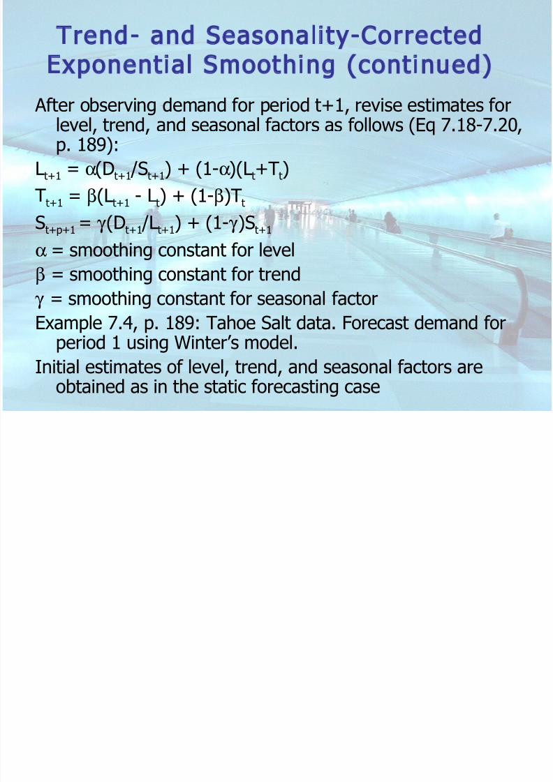
Trend- and Seasonality-CorrectedExponential Smoothing (continued)

After observing demand for period t+1, revise estimates forlevel, trend, and seasonal factors as follows (Eq 7.18-7.20,p. 189):

Lt+1 = α(Dt+1 /St+1) + (1-α)(Lt+Tt)

Tt+1 = β(Lt+1 - Lt) + (1-β)Tt

St+p+1 = γ (Dt+1 /Lt+1) + (1-γ )St+1

α = smoothing constant for levelβ = smoothing constant for trend

γ = smoothing constant for seasonal factorExample 7.4, p. 189: Tahoe Salt data. Forecast demand for

period 1 using Winter’s model.Initial estimates of level, trend, and seasonal factors are

obtained as in the static forecasting case



Trend- and Seasonality-Corrected ExponentialSmoothing Example (continued)

L0 = 18439 T0 = 524 S1=0.47, S2=0.68, S3=1.17, S4=1.67F1 = (L0 + T0)S1 = (18439+524)(0.47) = 8913

The observed demand for period 1 = D1 = 8000

Forecast error for period 1 = E1 = F1-D1 = 8913 - 8000 = 913

Assume α = 0.1, β=0.2, γ =0.1; revise estimates for level andtrend for period 1 and for seasonal factor for period 5

L1 = α(D1/S1)+(1-α)(L0+T0) = (0.1)(8000/0.47)+(0.9)(18439+524)=18769

T1 = β(L1-L0)+(1-β)T0 = (0.2)(18769-18439)+(0.8)(524) = 485S5 = γ (D1/L1)+(1-γ )S1 = (0.1)(8000/18769)+(0.9)(0.47) = 0.47

F2 = (L1+T1)S2 = (18769 + 485)(0.68) = 13093



Evaluation Non Seasonal Models

• Naïve cenderung harus dihindari

• MA akan cenderung bisa dipergunakan untuk estimate sales harian,dimana efek trend ataupun seasonal tidak terlalu nampak Sales /Produksi Harian

• E.S memiliki hasil yang responsive atau smoothing terhadap actual data.Tapi masalahnya adalah :

– Hanya tepat untuk one periods ahead – Asumsi bahwa data mengikuti kecenderungan eksponensial,

sehingga seharusnya nilai foracast adalah nilai tertinggi dari nilainialai aktual sebelumnya

• Holt dan Winter memiliki output yang baik, tapi kurang aplikatif karena

kesulitan dalam mengkonversikan nilai aktual dari alpha, beta, dangamma dalam kondisi aktual

• Trend hanya tepat dipergunakan apabila tidak terlihat adanyaseasonal dan data aktual jelas terlihat pola nail turunnya



• Mean Square Error – MSE / MSD

– Excel: =SUMSQ(error range)/COUNT(error range)

• Mean Absolute Percentage Error - MAPE

• R 2 - only for curve fitting model such as regression

• In general, the lower the error measure (BIAS, MAD, MSE) or the higherthe R 2, the better the forecasting model

n

(Error)

n

Forecast)-(Actual MSE

00

∑∑==

nActual

|Forecast-Actual|

MAPE∑

=

%000*

Evaluation of Forecasting Model



Measuring Accuracy, Forecast Errors

To compare different time series techniques or to selectthe “best” set of initial values for the parameters, use acombination of the the following four metrics:

Mean Absolute Deviation Most popular but

Mean Absolut Percent Error Should be used in tandem with MAD

Mean Square Error

Root Mean Square Error

n

FA

=MAD1

∑=

−n

i

ii

∑=

−n

i i

ii

n 1 AFA100 =MAPE

( )

n

FA

=MSE 1

2

∑=

−n

i

ii

MSERMSE =

R2 - only for curve fitting model such as regression

In general, the lower the error measure (MAD, MAPE, MSE, RMSE) or

the higher the R2, the better the forecasting model

MAD P bl D



MAD Problem Data

Question: What is the MAD value given

the forecast values in the table below?

Month Sales Forecast

1 220 n/a2 250 255

3 210 205

4 300 320

5 325 315

MAD P bl S l ti



MAD Problem Solution

Month Sales Forecast Abs Error 1 220 n/a

2 250 255 5

3 210 205 5

4 300 320 20

5 325 315 10

40

MAD =

A - F

n=

00

0=0

t tt=0

n

∑Note that by itself, the MAD

only lets us know the mean

error in a set of forecasts.

T ki Si l



Tracking Signal

The Tracking Signal or TS is a measure that

indicates whether the forecast average is keepingpace with any genuine upward or downwardchanges in demand.

Depending on the number of MAD’s selected, the TScan be used like a quality control chart indicating

when the model is generating too much error in itsforecasts.

TS is a monitoring system.

The TS formula is:

DeviationAbsoluteMean

ErrorsForecastof SumRunning=TS



Confidence Interval for Forecast

• If normal, the error can provide aconfidence interval for the forecast. – The % confidence interval for the forecast

-Using the standard deviation of the

forecast:

0

)( 0

−

−

=∑

n

F A

S t

t t

F

F S Z Forecast Y (%)±=



Example of Forecast Confidence Interval

• Using exponential smoothing in the previousexample, what is a 95% confidence interval forthe forecast for month 9?

alpha= .00

beta= .11

Month Demand

Excel exp

smooth

Text exp.

Smooth (A-F)^0

0 00 #N/A #N/A

0 11 .0000 .0000

0 00 .0000 .1111 00

0 11 .0000 .1111 0

0 00 .0000 .0000 .0000

0 00 .0000 .0000 .0000

0 00 .0000 .0000 .0000

0 00 .0000 .0000 .0000

0 00 .0000 .0000

sum= .00000

n= .000

n- =0 .000

Sf= .000

Start in month three to moreaccurately reflect the

exponential smoothing.

What is the interval

within which we are

95% confident that the

demand will be??

30.53+-1.96*5.11



HOT ISSUE IN FORECASTING

• Agrregate Forecasting is more accurate than single

forecast• For MTS, Colllaboration idea has been developed tominimizing error and uncertainty

• Watch out with Bullwhip phenomenon, when all part inyour Supply Chain doing a forecast with same purposes !

• Forecasting can become an operational activity, or justcan become a strategic activity ! Clearly your forecastinggoals !

• Combination of subjective and objective methods is themost methods that implement by many company

nowadays• Forecasting not just a software !!!!!



Final Thoughts- Big Picture

• Time is the enemy of the logistics plannerbecause time means uncertainty.

• Forecasting is often essential but think interms of reducing the importance / impact

of the forecast.• How ? Remember reduction in the cycle

time, demand management, Information

systems, and JIT ideas.

Types of Causal Forecasting



Types of Causal Forecasting

• Regression

• Econometric models

• Input-Output Models:

Causal Methods



Causal Methods

Linear Regression

• Causal methods are used when historical data areavailable and the relationship between the factor tobe forecasted and other external or internal factorscan be identified.

• Linear regression: A causal method in which onevariable (the dependent variable) is related to one ormore independent variables by a linear equation.

• Dependent variable: The variable that one wantsto forecast.

• Independent variables: Variables that areassumed to affect the dependent variable andthereby “cause” the results observed in the past.



Y Y

XX

Linear Regression Model

Observed valueObserved value

Y Y aa bb X X i i i i + +

Y Y aa bb X X i i i i +

Error Error

Error Error

Regression lineRegression line



Correlation

• Answers ‘how strong is the linearrelationship between 2 variables?’

• Coefficient of correlation used

• Used mainly for understanding



Coefficient of Correlation Values

-1.0-1.0 +1.0+1.000

PerfectPerfect

PositivePositive

CorrelationCorrelation

Increasing degree of Increasing degree of

negative correlationnegative correlation

-.5-.5 +.5+.5

PerfectPerfect

NegativeNegative

CorrelationCorrelationNoNo

CorrelationCorrelation

Increasing degree of Increasing degree of

positive correlationpositive correlation

Linear Regression



Line Formula

y = a + bx

y = the dependent variablea = the intercept

b = the slope of the line

x = the independent variable



Linear Regression Formulas

a = Y – bX b = ∑xy – nXY

∑x² - nX²

a = intercept

b = slope of the line

X = ∑x = mean of x

n the x data

Y = ∑y = mean of yn the y data

n = number of periods



Correlation

• Measures the strength of the relationshipbetween the dependent and independentvariable



Correlation Coefficient Formula

r = ______n∑xy - ∑x∑y______

√[n∑x² - (∑x)²][n∑y² - (∑y)²]

______________________________________ r = correlation coefficient

n = number of periods

x = the independent variabley = the dependent variable



Coefficient of Determination

• Another measure of the relationshipbetween the dependant and independentvariable

• Measures the percentage of variation in

the dependent (y) variable that isattributed to the independent (x) variabler = r²



• Causal forecasting is accurate and efficient

• When strong correlation exists the modelis very effective

• No forecasting method is 100% effective



Other Forecasting Methods

• Collaborative Planning Forecasting andReplenishment (CPFR)

– Establish collaborative relationships between buyers and sellers

– Create a joint business plan – Create a sales forecast

– Identify exceptions for sales forecast

– Resolve/collaborate on exception items

– Create order forecast – Identify exceptions for order forecast

– Resolve/collaborate on exception items

– Generate order



Forecasting as a Process

The forecast process itself, typically done on a monthly

basis, consists of structured steps. They often are

facilitated by someone who might be called a demand

manager, forecast analyst, or demand/supply planner.



Assignment

• Look at Chopra, chapter 7 page 203.

PPC Course new

Documents

Transcript of PPC Course new