Powerpoint TemplatesPage 1

Powerpoint Templates

Quantum Chemistry

Revisited

Powerpoint TemplatesPage 2

Wave Equation

Non Relativistic Limit

∇2𝜓 = ൬𝑘𝜔൰2 𝜕2𝜓𝜕𝑡2

𝜓ሺ𝑥,𝑦,𝑧,𝑡ሻ= 𝜓ሺ𝑥,𝑦,𝑧ሻ.𝜓ሺ𝑡ሻ Possible solution: Plane waves𝜓ሺ𝑡ሻ= 𝜓𝑜𝑒−𝑖𝜔𝑡

Powerpoint TemplatesPage 3

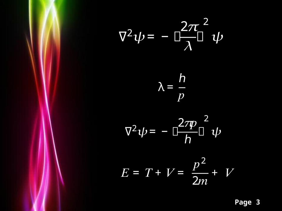
∇2𝜓 = −൬2𝜋𝜆൰

2 𝜓

λ= ℎ𝑝

∇2𝜓 = −൬2𝜋𝑝ℎ ൰

2 𝜓

𝐸= 𝑇+ 𝑉= 𝑝22𝑚+ 𝑉

Powerpoint TemplatesPage 4

𝑝= ඥ2𝑚(𝐸− 𝑉)

∇2𝜓 = −൬2𝜋ℎ൰

2 2𝑚(𝐸− 𝑉)𝜓

(− ℎ28𝜋2𝑚∇2 + 𝑉)𝜓 = 𝐸𝜓

Time Independent Schrödinger Equation

Powerpoint TemplatesPage 5

𝐸= ℎν= ℎ 𝜔2𝜋

𝜓ሺ𝑡ሻ= 𝜓𝑜𝑒−𝑖𝜔𝑡

𝑑𝜓ሺ𝑡ሻ𝑑𝑡 = −𝑖2𝜋𝐸ℎ 𝜓𝑜𝑒−𝑖𝜔𝑡

𝑖 ℎ2𝜋𝑑𝑑𝑡𝜓ሺ𝑡ሻ= 𝐸𝜓ሺ𝑡ሻ Time dependent Schrödinger Equation

Powerpoint TemplatesPage 6

ቆ− ℎ28𝜋2𝑚∇2 + 𝑉ቇ𝜓(𝑥,𝑦,𝑧)𝜓(𝑡) = 𝑖 ℎ2𝜋𝑑𝑑𝑡𝜓(𝑥,𝑦,𝑧)𝜓(𝑡)

Lousy relativistic equation

2nd derivative in space

1st derivative in time

Many fathers equation

(Klein, Fock, Schrödinger, de Broglie, ...)

Klein-Gordon Equation (1926)

Powerpoint TemplatesPage 7

(E – V)2 = p2c2 + m2c4

ℎ2𝑐24𝜋2 𝛿2𝜑(𝑞)𝛿𝑞2 +ሾሺ𝐸− 𝑉ሻ2 − 𝑚𝑜2𝑐4ሿ𝜑ሺ𝑞ሻ= 0

ℎ2𝑐24𝜋2 𝛿2𝜓ሺ𝑞,𝑡ሻ𝛿𝑞2 − ℎ24𝜋2 𝛿2𝜓ሺ𝑞,𝑡ሻ𝛿𝑡2 – 𝑖ℎ𝑉𝜋 𝛿𝜓(𝑞,𝑡)𝛿𝑡 + ሺ𝑉2 − 𝑚𝑜2𝑐4ሻ𝜓(𝑞,𝑡) = 0

Free Electron (V = 0)

ℎ2𝑐24𝜋2 𝛿2𝜓ሺ𝑞,𝑡ሻ𝛿𝑞2 − ℎ24𝜋2 𝛿2𝜓ሺ𝑞,𝑡ሻ𝛿𝑡2 − 𝑚𝑜2𝑐4 𝜓(𝑞,𝑡) = 0

Powerpoint TemplatesPage 8

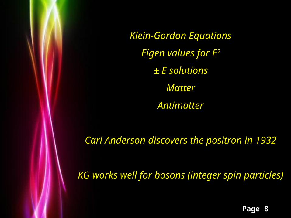
Klein-Gordon Equations

Eigen values for E2

± E solutions

Matter

Antimatter

Carl Anderson discovers the positron in 1932

KG works well for bosons (integer spin particles)

Powerpoint TemplatesPage 9

(𝑎𝛻+ 𝑏𝑖𝑐 𝑑𝑑𝑡)2 = 𝑎2𝛻2 − 𝑏2 1𝑐2 𝑑𝑑𝑡2

a = b = 1

ab + ba = 0

𝑎 = ቂ1 00 −1ቃ 𝑏 = ቂ0 11 0ቃ 𝑜𝑟 𝑐 = ቂ0 −𝑖𝑖 0ቃ

Powerpoint TemplatesPage 10

𝛼1 = 0 00 0 0 11 00 11 0 0 00 0 𝛼2 = 0 00 0 0 −𝑖𝑖 00 −𝑖𝑖 0 0 00 0

𝛼3 = 0 00 0 1 00 −11 00 −1 0 00 0 𝛽 = 1 00 1 0 00 00 00 0 −1 00 −1

3 dimensions and time

Powerpoint TemplatesPage 11

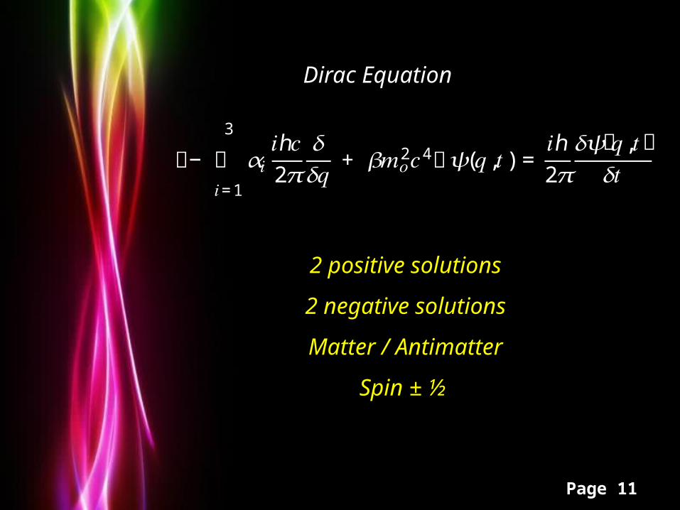
൭− 𝛼𝑖 𝑖ℎ𝑐2𝜋 𝛿𝛿𝑞3

𝑖=1 + 𝛽𝑚𝑜2𝑐4൱𝜓(𝑞,𝑡) = 𝑖ℎ2𝜋𝛿𝜓ሺ𝑞,𝑡ሻ𝛿𝑡

Dirac Equation

2 positive solutions

2 negative solutions

Matter / Antimatter

Spin ± ½

Powerpoint TemplatesPage 12

𝜎1 = ቂ1 00 −1ቃ 𝜎2 = ቂ0 11 0ቃ 𝜎3 = ቂ0 −𝑖𝑖 0ቃ Pauli Matrices

𝑝= −𝑖 ℎ2𝜋∇− 𝑒𝑐𝐴

𝜎.𝑝= 𝜎.(−𝑖 ℎ2𝜋∇− 𝑒𝑐𝐴)

Powerpoint TemplatesPage 13

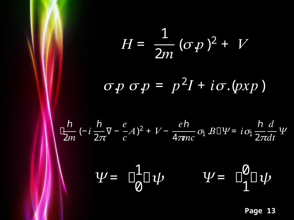
𝐻= 12𝑚(𝜎.𝑝)2 + 𝑉

𝜎.𝑝 𝜎.𝑝= 𝑝2𝐼+ 𝑖𝜎.(𝑝𝑥𝑝)

ℎ2𝑚(−𝑖 ℎ2𝜋∇− 𝑒𝑐𝐴)2 + 𝑉− 𝑒ℎ4𝜋𝑚𝑐𝜎1.𝐵൨𝛹= 𝑖𝜎1 ℎ2𝜋𝑑𝑑𝑡𝛹

𝛹= ቀ10ቁ𝜓 𝛹= ቀ01ቁ𝜓

Powerpoint TemplatesPage 14

ቆ− ℎ28𝜋2𝑚 𝛿2𝛿𝑞2 + 𝑉ቇ𝜓ሺ𝑞,𝑡ሻ= 𝑖 ℎ2𝜋 𝛿𝜓(𝑞,𝑡)𝛿𝑡

ቆ− ℎ28𝜋2𝑚 𝛿2𝛿𝑞2 + 𝑉ቇ𝜓∗ሺ𝑞,𝑡ሻ= − 𝑖 ℎ2𝜋 𝛿𝜓∗(𝑞,𝑡)𝛿𝑡

𝜓∗ቆ− ℎ28𝜋2𝑚 𝛿2𝛿𝑞2 + 𝑉ቇ𝜓 = 𝜓∗𝑖 ℎ2𝜋 𝛿𝜓𝛿𝑡

𝜓ቆ− ℎ28𝜋2𝑚 𝛿2𝛿𝑞2 + 𝑉ቇ𝜓∗= − 𝜓𝑖 ℎ2𝜋 𝛿𝜓∗𝛿𝑡

Powerpoint TemplatesPage 15

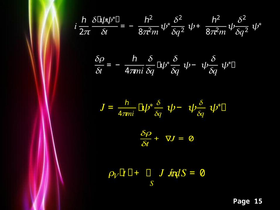
𝑖 ℎ2𝜋 𝛿ሾ𝜓𝜓∗ሿ𝛿𝑡 = − ℎ28𝜋2𝑚𝜓∗ 𝛿2𝛿𝑞2 𝜓+ ℎ28𝜋2𝑚𝜓 𝛿2𝛿𝑞2 𝜓∗

𝛿𝜌𝛿𝑡 = − ℎ4𝜋𝑚𝑖 𝛿𝛿𝑞𝜓∗ 𝛿𝛿𝑞 𝜓− 𝜓 𝛿𝛿𝑞 𝜓∗൨

𝐽= ℎ4𝜋𝑚𝑖 ቂ𝜓∗ 𝛿𝛿𝑞 𝜓− 𝜓 𝛿𝛿𝑞 𝜓∗ቃ 𝛿𝜌𝛿𝑡 + ∇𝐽= 0

𝜌𝑉ሺ𝑡ሻ+ න 𝐽𝑆 .𝑛ሬԦ𝑑𝑆= 0

Powerpoint TemplatesPage 16

There cant be flow in pure real and pure imaginary wave

functions.

In stationary states the flow is either zero or constant.

div D = ρ implies that stationary states create static

electric fields.

rot H = J + D/t implies that stationary states with J≠0

create static magnetic fields.

Static magnetic fields induce currents J which create

induced magnetic fields.

Time dependent magnetic fields induce time dependent

electric fields (rot E = - B/t), which means time

dependent charge densities to which correspond non

stationary states.