Power Utility Maximization in Constrained

Exponential Lévy Models

Marcel NutzETH Zurich, Department of Mathematics, 8092 Zurich, Switzerland

marcel.nutz@math.ethz.ch

This Version: September 1, 2010.

Abstract

We study power utility maximization for exponential Lévy modelswith portfolio constraints, where utility is obtained from consumptionand/or terminal wealth. For convex constraints, an explicit solution interms of the Lévy triplet is constructed under minimal assumptions bysolving the Bellman equation. We use a novel transformation of themodel to avoid technical conditions. The consequences for q-optimalmartingale measures are discussed as well as extensions to non-convexconstraints.

Keywords power utility, Lévy process, constraints, dynamic programming.AMS 2000 Subject Classi�cations Primary 91B28, secondary 60G51.JEL Classi�cation G11, C61.

Acknowledgements. Financial support by Swiss National Science Founda-tion Grant PDFM2-120424/1 is gratefully acknowledged. The author thanksMartin Schweizer, Josef Teichmann and two anonymous referees for detailedcomments on an earlier version of the manuscript.

1 Introduction

A classical problem of mathematical �nance is the maximization of expectedutility from consumption and/or from terminal wealth for an investor. Weconsider the special case when the asset prices follow an exponential Lévyprocess and the investor's preferences are given by a power utility function.This problem was �rst studied by Merton [20] for drifted geometric Brow-nian motion and by Mossin [21] and Samuelson [25] for the discrete-timeanalogues. A consistent observation was that when the asset returns arei.i.d., the optimal portfolio and consumption are given by a constant and adeterministic function, respectively. This result was subsequently extendedto various classes of Lévy models (see, among others, Foldes [8], Framstadet al. [9], Benth et al. [2, 3], Kallsen [14]) and its general validity was readily

1

conjectured. We note that the existence of an optimal strategy is known alsofor much more general models (see Karatzas and �itkovi¢ [16]), but a priori

that strategy is some stochastic process without a constructive description.We prove this conjecture for general Lévy models under minimal assump-

tions; in addition, we consider the case where the choice of the portfolio isconstrained to a convex set. The optimal investment portfolio is character-ized as the maximizer of a deterministic concave function g de�ned in termsof the Lévy triplet; and the maximum of g yields the optimal consumption.Moreover, the Lévy triplet characterizes the �niteness of the value function,i.e., the maximal expected utility. We also draw the conclusions for theq-optimal equivalent martingale measures that are linked to utility maxi-mization by convex duality (q ∈ (−∞, 1) ∖ {0}); this results in an explicitexistence characterization and a formula for the density process. Finally,some generalizations to non-convex constraints are studied.

Our method consists in solving the Bellman equation, which was intro-duced for general semimartingale models in Nutz [23]. In the Lévy setting,this equation reduces to a Bernoulli ordinary di�erential equation. Thereare two main mathematical di�culties. The �rst one is to construct themaximizer for g, i.e., the optimal portfolio. The necessary compactness isobtained from a minimal no-free-lunch condition (�no unbounded increas-ing pro�t�) via scaling arguments which were developed by Kardaras [17]for log-utility. In our setting these arguments require certain integrabilityproperties of the asset returns. Without compromising the generality, inte-grability is achieved by a linear transformation of the model which replacesthe given assets by certain portfolios. We construct the maximizer for g inthe transformed model and then revert to the original one.

The second di�culty is to verify the optimality of the constructed con-sumption and investment portfolio. Here we use the general veri�cationtheory of [23] and exploit a well-known property of Lévy processes, namelythat any Lévy local martingale is a true martingale.

This paper is organized as follows. The next section speci�es the opti-mization problem and the notation related to the Lévy triplet. We also recallthe no-free-lunch condition NUIPC and the opportunity process. Section 3states the main result for utility maximization under convex constraints andrelates the triplet to the �niteness of the value function. The transforma-tion of the model is described in Section 4 and the main theorem is provedin Section 5. Section 6 gives the application to q-optimal measures whilenon-convex constraints are studied in Section 7. Related literature is dis-cussed in the concluding Section 8 as this necessitates technical terminologyintroduced in the body of the paper.

2

2 Preliminaries

The following notation is used. If x, y ∈ ℝ are reals, x+ = max{x, 0} andx ∧ y = min{x, y}. We set 1/0 := ∞ where necessary. If z ∈ ℝd is ad-dimensional vector, zi is its ith coordinate and z⊤ its transpose. GivenA ⊆ ℝd, A⊥ denotes the Euclidean orthogonal complement and A is saidto be star-shaped (with respect to the origin) if �A ⊆ A for all � ∈ [0, 1].If X is an ℝd-valued semimartingale and � ∈ L(X) is an ℝd-valued pre-dictable integrand, the vector stochastic integral is a scalar semimartingalewith initial value zero and denoted by

∫� dX or by � ∙ X. Relations between

measurable functions hold almost everywhere unless otherwise stated. Ourreference for any unexplained notion or notation from stochastic calculus isJacod and Shiryaev [12].

2.1 The Optimization Problem

We �x the time horizon T ∈ (0,∞) and a probability space (Ω,ℱ , P ) with a�ltration (ℱt)t∈[0,T ] satisfying the usual assumptions of right-continuity andcompleteness, as well as ℱ0 = {∅,Ω} P -a.s. We consider an ℝd-valued Lévy

process R = (R1, . . . , Rd) with R0 = 0. That is, R is a càdlàg semimartingalewith stationary independent increments as de�ned in [12, II.4.1(b)]. It is notrelevant for us whether R generates the �ltration. The stochastic exponentialS = ℰ(R) = (ℰ(R1), . . . , ℰ(Rd)) represents the discounted price processes ofd risky assets, while R stands for their returns. If one wants to model onlypositive prices, one can equivalently use the ordinary exponential (see, e.g.,[14, Lemma 4.2]). Our agent also has a bank account paying zero interest athis disposal.

The agent is endowed with a deterministic initial capital x0 > 0. Atrading strategy is a predictable R-integrable ℝd-valued process �, wherethe ith component is interpreted as the fraction of wealth (or the portfolioproportion) invested in the ith risky asset.

We want to consider two cases. Either consumption occurs only at theterminal time T (utility from �terminal wealth� only); or there is intermediateconsumption plus a bulk consumption at the time horizon. To unify thenotation, we de�ne

� :=

{1 in the case with intermediate consumption,

0 otherwise.

It will be convenient to parametrize the consumption strategies as a fractionof the current wealth. A propensity to consume is a nonnegative optionalprocess � satisfying

∫ T0 �s ds < ∞ P -a.s. The wealth process X(�, �) corre-

sponding to a pair (�, �) is de�ned by the stochastic exponential

X(�, �) = x0ℰ(� ∙ R− �

∫�s ds

).

3

In particular, the number of shares of the ith asset held in the portfolio isthen given by �iX(�, �)−/S

i− (on the set {Si− ∕= 0}).

Let C ⊆ ℝd be a set containing the origin; we refer to C as �the con-straints�. The set of (constrained) admissible strategies is

A(x0) :={

(�, �) : X(�, �) > 0 and �t(!) ∈ C for all (!, t) ∈ Ω× [0, T ]}.

We �x the initial capital x0 and usually write A for A(x0). Given (�, �) ∈ A,c := �X(�, �) is the corresponding consumption rate and X = X(�, �)satis�es the self-�nancing condition Xt = x0 +

∫ t0 Xs−�s dRs − �

∫ t0 cs ds.

Let p ∈ (−∞, 0) ∪ (0, 1). We use the power utility function

U(x) := 1px

p, x ∈ (0,∞)

to model the preferences of the agent. The constant � := (1 − p)−1 > 0 isthe relative risk tolerance of U . Note that we exclude the logarithmic utility,which corresponds to p = 0 and for which the optimal strategies are knownexplicitly even for semimartingale models (see Karatzas and Kardaras [15]).

Let (�, �) ∈ A and X = X(�, �), c = �X. The corresponding expected

utility is E[�∫ T

0 U(ct) dt+ U(XT )]. The value function is given by

u(x0) := supA(x0)

E[�

∫ T

0U(ct) dt+ U(XT )

],

where the supremum is taken over all (c,X) which correspond to some(�, �) ∈ A(x0). We say that the utility maximization problem is �nite ifu(x0) <∞; this always holds if p < 0 as then U < 0. If u(x0) <∞, (�, �) isoptimal if the corresponding (c,X) satisfy E

[�∫ T

0 U(ct) dt+U(XT )]

= u(x0).

2.2 Lévy Triplet, Constraints, No-Free-Lunch Condition

Let (bR, cR, FR) be the Lévy triplet of R with respect to some �xed cut-o�function ℎ : ℝd → ℝd (i.e., ℎ is bounded and ℎ(x) = x in a neighborhoodof x = 0). This means that bR ∈ ℝd, cR ∈ ℝd×d is a nonnegative de�nitematrix, and FR is a Lévy measure on ℝd, i.e., FR{0} = 0 and∫

ℝd

1 ∧ ∣x∣2 FR(dx) <∞. (2.1)

The process R can be represented as

Rt = bRt+Rct + ℎ(x) ∗ (�Rt − �Rt ) + (x− ℎ(x)) ∗ �Rt .

Here �R is the integer-valued random measure associated with the jumpsof R and �Rt = tFR is its compensator. Moreover, Rc is the continuousmartingale part, in fact, Rct = �Wt, where � ∈ ℝd×d satis�es ��⊤ = cR and

4

W is a d-dimensional standard Brownian motion. We refer to [12, II.4] orSato [26] for background material concerning Lévy processes.

We introduce some subsets of ℝd to be used in the sequel; the terminologyfollows [17]. The �rst two are related to the �budget constraint� X(�, �) > 0.The natural constraints are given by

C 0 :={y ∈ ℝd : FR

[x ∈ ℝd : y⊤x < −1

]= 0}

;

clearly C 0 is closed, convex, and contains the origin. We also consider theslightly smaller set

C 0,∗ :={y ∈ ℝd : FR

[x ∈ ℝd : y⊤x ≤ −1

]= 0}.

It is convex, contains the origin, and its closure equals C 0, but it is a propersubset in general. The meaning of these sets is explained by

Lemma 2.1. A process � ∈ L(R) satis�es ℰ(� ∙ R) ≥ 0 (> 0) if and only if

� takes values in C 0 (C 0,∗) P ⊗ dt-a.e.

See, e.g., [23, Lemma 2.5] for the proof. We observe that C 0,∗ correspondsto the admissible portfolios; however, the set C 0 also turns out to be useful,due to the closedness.

The linear space of null-investments is de�ned by

N :={y ∈ ℝd : y⊤bR = 0, y⊤cR = 0, FR[x : y⊤x ∕= 0] = 0

}.

Then H ∈ L(R) satis�es H ∙ R ≡ 0 if and only if H takes values in NP ⊗ dt-a.e. In particular, two portfolios � and �′ generate the same wealthprocess if and only if � − �′ is N -valued.

We recall the set 0 ∈ C ⊆ ℝd of portfolio constraints. The set J ⊆ ℝdof immediate arbitrage opportunities is de�ned by

J ={y : y⊤cR = 0, FR[y⊤x < 0] = 0, y⊤bR−

∫y⊤ℎ(x)FR(dx) ≥ 0

}∖N .

Note that for y ∈ J , the process y⊤R is increasing and nonconstant. Fora subset G of ℝd, the recession cone is given by G :=

∩a≥0 aG. Now the

condition NUIPC (no unbounded increasing pro�t) can be de�ned by

NUIPC ⇐⇒ J ∩ C = ∅

(cf. [17, Theorem 4.5]). This is equivalent to J ∩ (C ∩ C 0) = ∅ becauseJ ⊆ C 0, and it means that if a strategy leads to an increasing nonconstantwealth process, then that strategy cannot be scaled arbitrarily. This is aminimal no-free lunch condition (cf. Remark 3.4(c)); we refer to [17] formore information about free lunches in exponential Lévy models. We give asimple example to illustrate the objects.

5

Example 2.2. Assume there is only one asset (d = 1), that its price isstrictly positive, and that it can jump arbitrarily close to zero and arbitrarilyhigh. In formulas, FR(−∞,−1] = 0 and for all " > 0, FR(−1,−1 + "] > 0and FR["−1,∞) > 0.

Then C 0 = C 0,∗ = [0, 1] and N = {0}. In this situation NUIPC issatis�ed for any set C , both because J = ∅ and because C 0 = {0}. If theprice process is merely nonnegative and FR{−1} > 0, then C 0,∗ = [0, 1)while the rest stays the same.

In fact, most of the scalar models presented in Schoutens [27] correspondto the �rst part of Example 2.2 for nondegenerate choices of the parameters.

2.3 Opportunity Process

Assume u(x0) < ∞ and let (�, �) ∈ A. For �xed t ∈ [0, T ], the set of�compatible� controls is A(�, �, t) :=

{(�, �) ∈ A : (�, �) = (�, �) on [0, t]

}.

By [24, Proposition 3.1, Remark 3.7] there exists a unique càdlàg semimartin-gale L, called opportunity process, such that

Lt1p

(Xt(�, �)

)p= ess supA(�,�,t)

E[�

∫ T

tU(cs) ds+ U(XT )

∣∣∣ℱt],where the supremum is taken over all consumption and wealth pairs (c, X)corresponding to some (�, �) ∈ A(�, �, t). The right hand side above isknown as the value process of our control problem and its factorization ap-pearing on the left hand side is a consequence of the p-homogeneity of U .We shall see that in the present (Markovian) Lévy setting, the opportunityprocess is simply a deterministic function. In particular, the value processcoincides with the more familiar �dynamic value function� in the sense ofMarkovian dynamic programming, ut(x) = Lt

1px

p, evaluated at Xt(�, �).

3 Main Result

We can now formulate the main theorem for the convex-constrained case; theproofs are given in the two subsequent sections. We consider the followingconditions (not to be understood as standing assumptions).

Assumptions 3.1.

(i) C is convex.

(ii) The orthogonal projection of C ∩ C 0 onto N ⊥ is closed.

(iii) NUIPC holds.

(iv) u(x0) <∞, i.e., the utility maximization problem is �nite.

6

To state the result, we de�ne for y ∈ C 0 the deterministic function

g(y) := y⊤bR + (p−1)2 y⊤cRy +

∫ℝd

{p−1(1 + y⊤x)p − p−1 − y⊤ℎ(x)

}FR(dx).

(3.1)As we will see later, this concave function is well de�ned with values inℝ ∪ {sign(p)∞}.

Theorem 3.2. Under Assumptions 3.1, there exists an optimal strategy

(�, �) such that � is a constant vector and � is deterministic. Here � is

characterized by

� ∈ arg maxC∩C 0 g

and, in the case with intermediate consumption,

�t = a((1 + a)ea(T−t) − 1

)−1,

where a := p1−p maxC∩C 0 g. The opportunity process is given by

Lt =

{exp

(a(1− p)(T − t)

)without intermediate consumption,

ap−1[(1 + a)ea(T−t) − 1

]1−pwith intermediate consumption.

Remark 3.3 ([23, Remark 3.3]). The propensity to consume � is unique.The optimal portfolio � and arg maxC∩C 0 g are unique modulo N ; i.e., if �∗

is another optimal portfolio (or maximizer), then �− �∗ takes values in N .Equivalently, the wealth processes coincide.

We comment on Assumptions 3.1.

Remark 3.4. (a) Convexity of C is of course not necessary to have asolution. We give some generalizations in Section 7.

(b) The projection of C ∩ C 0 onto N ⊥ should be understood as �e�ec-tive domain� of the optimization problem. Without the closedness in (ii),there are examples with non-existence of an optimal strategy even for driftedBrownian motion and closed convex cone constraints; see Example 3.5 below.One can note that closedness of C implies (ii) if N ⊆ C and C is convex(as this implies C = C + N , see [17, Remark 2.4]). Similarly, (ii) holdswhenever the projection of C to N ⊥ is closed: if Π denotes the projector,C 0 = C 0 +N yields Π(C ∩C 0) = (ΠC )∩C 0 and C 0 is closed. This includesthe cases where C is closed and polyhedral, or compact.

(c) Suppose that NUIPC does not hold. If p ∈ (0, 1), it is obvious thatu(x0) = ∞. If p < 0, there exists no optimal strategy, essentially becauseadding a suitable arbitrage strategy would always yield a higher expectedutility. See [15, Proposition 4.19] for a proof.

(d) If u(x0) = ∞, either there is no optimal strategy, or there are in-�nitely many strategies yielding in�nite expected utility. It would be incon-venient to call the latter optimal. Indeed, using that u(x0/2) =∞, one can

7

typically construct such strategies which also exhibit intuitively suboptimalbehavior (such as throwing away money by a �suicide strategy�; see Harrisonand Pliska [11, �6.1]). Hence we require (iv) to have a meaningful solutionto our problem�the relevant question is how to characterize this conditionin terms of the model.

The following example illustrates how non-existence of an optimal portfo-lio may occur when Assumption 3.1(ii) is violated. It is based on Czichowskyet al. [7, �2.2], where the authors give an example of a set of stochastic inte-grals which is not closed in the semimartingale topology. We denote by ej ,1 ≤ j ≤ d the unit vectors in ℝd, i.e., eij = �ij .

Example 3.5 (� = 0). Let W be a standard Brownian motion in ℝ3 and

� =

⎛⎝1 0 00 1 −10 −1 1

⎞⎠ ; C ={y ∈ ℝ3 :

∣∣y1∣∣2 +

∣∣y2∣∣2 ≤ ∣∣y3

∣∣2, y3 ≥ 0}.

Let Rt = bt + �Wt, where b := e1 is orthogonal to ker�⊤ = ℝ(0, 1, 1)⊤.Thus N = ker�⊤ and N ⊥ is spanned by e1 and e2− e3. The closed convexcone C is �leaning� against the plane N ⊥ and the orthogonal projection ofC onto N ⊥ is an open half-plane plus the origin. The vectors �e1 with� ∈ ℝ ∖ {0} are not contained in this half-plane but in its closure.

The optimal portfolio � for the unconstrained problem lies on this bound-ary. Indeed, NUIPℝ3 holds and Theorem 3.2 yields � = �(��⊤)−1e1 = �e1,where � = (1 − p)−1. This is simply Merton's optimal portfolio in themarket consisting only of the �rst asset. By construction we �nd vectors�n ∈ C whose projections to N ⊥ converge to � and it is easy to see thatE[U(XT (�n))] → E[U(XT (�))]. Hence the value functions for the con-strained and the unconstrained problem are identical. Since the solution �of the unconstrained problem is unique modulo N , this implies that if theconstrained problem has a solution, it has to agree with �, modulo N . But({�}+ N ) ∩ C = ∅, so there is no solution.

The rest of the section is devoted to the characterization of Assump-tion 3.1(iv) by the jump characteristic FR and the set C ; this is intimatelyrelated to the moment condition∫

{∣x∣>1}∣x∣p FR(dx) <∞. (3.2)

We start with a partial result; again ej , 1 ≤ j ≤ d denote the unit vectors.

Proposition 3.6. Let p ∈ (0, 1).

(i) Under Assumptions 3.1(i)-(iii), (3.2) implies u(x0) <∞.

(ii) If ej ∈ C ∩ C 0,∗ for all 1 ≤ j ≤ d, then u(x0) <∞ implies (3.2).

8

By Lemma 2.1 the jth asset has a positive price if and only if ej ∈ C 0,∗.Hence we have the following consequence of Proposition 3.6.

Corollary 3.7. In an unconstrained exponential Lévy model with positive

asset prices satisfying NUIPℝd , u(x0) <∞ is equivalent to (3.2).

The implication u(x0) <∞⇒ (3.2) is essentially true also in the generalcase; more precisely, it holds in an equivalent model. As a motivation, con-sider the case where either C = {0} or C 0 = {0}. The latter occurs, e.g., ifd = 1 and the asset has jumps which are unbounded in both directions. Thenthe statement u(x0) < ∞ carries no information about R because � ≡ 0 isthe only admissible portfolio. On the other hand, we are not interested inassets that cannot be traded, and may as well remove them from the model.This is part of the following result.

Proposition 3.8. There exists a linear transformation (R, C ) of the model

(R,C ), which is equivalent in that it admits the same wealth processes, and

has the following properties:

(i) the prices are strictly positive,

(ii) the wealth can be invested in each asset (i.e., � ≡ ej is admissible),

(iii) if u(x0) < ∞ holds for (R,C ), it holds also in the model (R, C ) and∫{∣x∣>1} ∣x∣

p F R(dx) <∞.

The details of the construction are given in the next section, where wealso show that Assumptions 3.1 carry over to (R, C ).

4 Transformation of the Model

This section contains the announced linear transformation of the marketmodel. Assumptions 3.1 are not used. We �rst describe how any lineartransformation a�ects our objects.

Lemma 4.1. Let Λ be a d×d-matrix and de�ne R := ΛR. Then R is a Lévy

process with triplet bR = ΛbR, cR = ΛcRΛ⊤ and F R(⋅) = FR(Λ−1⋅). More-

over, the corresponding natural constraints and null-investments are given

by C 0 := (ΛT )−1C 0 and N := (ΛT )−1N and the corresponding function gsatis�es g(z) = g(Λ⊤z).

The proof is straightforward and omitted. Of course, Λ−1 refers tothe preimage if Λ is not invertible. Given Λ, we keep the notation fromLemma 4.1 and introduce also C := (ΛT )−1C as well as C 0,∗ := (ΛT )−1C 0,∗.

Theorem 4.2. There exists a d× d-matrix Λ such that for all 1 ≤ j ≤ d,(i) ΔRj > −1 up to evanescence,

(ii) ej ∈ C ∩ C 0,∗,

9

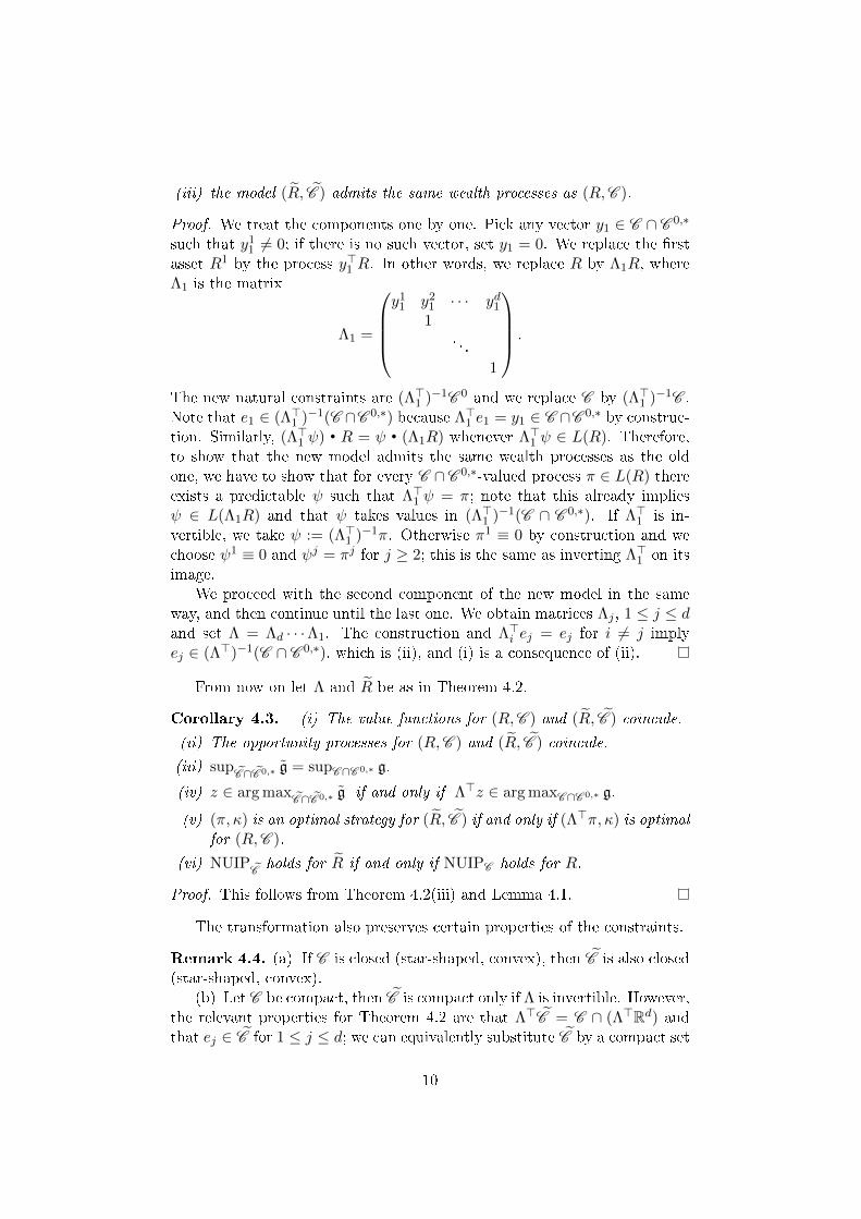
(iii) the model (R, C ) admits the same wealth processes as (R,C ).

Proof. We treat the components one by one. Pick any vector y1 ∈ C ∩ C 0,∗

such that y11 ∕= 0; if there is no such vector, set y1 = 0. We replace the �rst

asset R1 by the process y⊤1 R. In other words, we replace R by Λ1R, whereΛ1 is the matrix

Λ1 =

⎛⎜⎜⎜⎝y1

1 y21 ⋅ ⋅ ⋅ yd11

. . .1

⎞⎟⎟⎟⎠ .

The new natural constraints are (Λ⊤1 )−1C 0 and we replace C by (Λ⊤1 )−1C .Note that e1 ∈ (Λ⊤1 )−1(C ∩C 0,∗) because Λ⊤1 e1 = y1 ∈ C ∩C 0,∗ by construc-tion. Similarly, (Λ⊤1 ) ∙ R = ∙ (Λ1R) whenever Λ⊤1 ∈ L(R). Therefore,to show that the new model admits the same wealth processes as the oldone, we have to show that for every C ∩C 0,∗-valued process � ∈ L(R) thereexists a predictable such that Λ⊤1 = �; note that this already implies ∈ L(Λ1R) and that takes values in (Λ⊤1 )−1(C ∩ C 0,∗). If Λ⊤1 is in-vertible, we take := (Λ⊤1 )−1�. Otherwise �1 ≡ 0 by construction and wechoose 1 ≡ 0 and j = �j for j ≥ 2; this is the same as inverting Λ⊤1 on itsimage.

We proceed with the second component of the new model in the sameway, and then continue until the last one. We obtain matrices Λj , 1 ≤ j ≤ dand set Λ = Λd ⋅ ⋅ ⋅Λ1. The construction and Λ⊤i ej = ej for i ∕= j implyej ∈ (Λ⊤)−1(C ∩ C 0,∗), which is (ii), and (i) is a consequence of (ii).

From now on let Λ and R be as in Theorem 4.2.

Corollary 4.3. (i) The value functions for (R,C ) and (R, C ) coincide.

(ii) The opportunity processes for (R,C ) and (R, C ) coincide.

(iii) supC∩C 0,∗ g = supC∩C 0,∗ g.

(iv) z ∈ arg maxC∩C 0,∗ g if and only if Λ⊤z ∈ arg maxC∩C 0,∗ g.

(v) (�, �) is an optimal strategy for (R, C ) if and only if (Λ⊤�, �) is optimal

for (R,C ).

(vi) NUIPCholds for R if and only if NUIPC holds for R.

Proof. This follows from Theorem 4.2(iii) and Lemma 4.1.

The transformation also preserves certain properties of the constraints.

Remark 4.4. (a) If C is closed (star-shaped, convex), then C is also closed(star-shaped, convex).

(b) Let C be compact, then C is compact only if Λ is invertible. However,the relevant properties for Theorem 4.2 are that Λ⊤C = C ∩ (Λ⊤ℝd) andthat ej ∈ C for 1 ≤ j ≤ d; we can equivalently substitute C by a compact set

10

having these properties. If Λ⊤ is considered as a mapping ℝd → Λ⊤ℝd , itadmits a continuous right-inverse f , and (Λ⊤)−1C = f(C ∩Λ⊤ℝd)+ker(Λ⊤).Here f(C ∩ Λ⊤ℝd) is compact and contained in Br = {x ∈ ℝd : ∣x∣ ≤ r}for some r ≥ 1. The set C :=

[f(C ∩ Λ⊤ℝd) + ker(Λ⊤)

]∩ Br has the two

desired properties.

Next, we deal with the projection of C ∩ C 0 onto N ⊥. We begin witha �coordinate-free� description for its closedness; it can be seen as a simplestatic version of the main result in Czichowsky and Schweizer [6].

Lemma 4.5. Let D ⊆ ℝd be a nonempty set and let D ′ be its orthogonal

projection onto N ⊥. Then D ′ is closed in ℝd if and only if {y⊤RT : y ∈ D}is closed for convergence in probability.

Proof. Recalling the de�nition of N , we may assume that D = D ′. If (yn)is a sequence in D with some limit y∗, clearly y⊤nRT → y⊤∗ RT in probability.If {y⊤RT : y ∈ D} is closed, it follows that y∗ ∈ D because D ∩N = {0};hence D is closed.

Conversely, let yn ∈ D and assume y⊤nRT → Y in probability for someY ∈ L0(ℱ). With D ∩N = {0} it follows that (yn) is bounded, therefore, ithas a subsequence which converges to some y∗. If D is closed, then y∗ ∈ Dand we conclude that Y = y⊤∗ RT , showing closedness in probability.

Lemma 4.6. Assume that C ∩C 0,∗ is dense in C ∩C 0. Then the orthogonal

projection of C ∩ C 0 onto N ⊥ is closed if and only if this holds for C ∩ C 0

and N ⊥.

Proof. (i) Recall the construction of Λ = Λd ⋅ ⋅ ⋅Λ1 from the proof of The-orem 4.2. Assume �rst that Λ = Λi for some 1 ≤ i ≤ d. In a �rst step, weshow

Λ⊤(C ∩ C 0) = C ∩ C 0. (4.1)

By construction, either Λ is invertible, in which case the claim is clear,or otherwise Λ⊤ is the orthogonal projection of ℝd onto the hyperplaneHi = {y ∈ ℝd : yi = 0} and C ∩ C 0,∗ ⊆ Hi. By the density assumption itfollows that C ∩ C 0 ⊆ Hi. Thus (Λ⊤)−1(C ∩ C 0) = C ∩ C 0 +H⊥i , the sumbeing orthogonal, and Λ⊤[(Λ⊤)−1(C ∩ C 0)] = C ∩ C 0 as claimed. We alsonote that

(Λ⊤)−1(C ∩ C 0,∗) ⊆ (Λ⊤)−1(C ∩ C 0) is dense. (4.2)

Using (4.1) we have {y⊤RT : y ∈ C ∩C 0} = {y⊤RT : y ∈ C ∩ C 0} and nowthe result follows from Lemma 4.5, for the special case Λ = Λi.

(ii) In the general case, we have C ∩ C 0 = (Λ⊤d )−1 ∘⋅ ⋅ ⋅∘(Λ⊤1 )−1(C ∩C 0).We apply part (i) successively to Λ1, . . . ,Λd to obtain the result, here (4.2)ensures that the density assumption is satis�ed in each step.

11

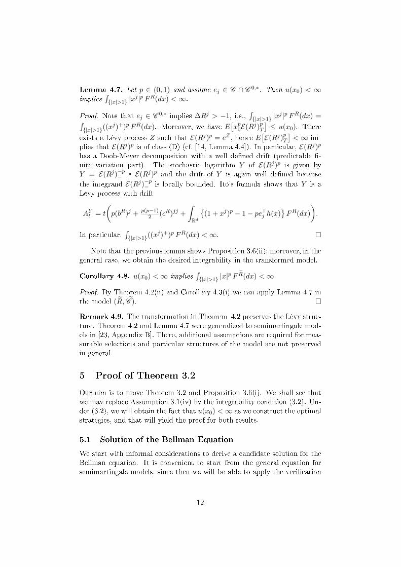
Lemma 4.7. Let p ∈ (0, 1) and assume ej ∈ C ∩ C 0,∗. Then u(x0) < ∞implies

∫{∣x∣>1} ∣x

j ∣p FR(dx) <∞.

Proof. Note that ej ∈ C 0,∗ implies ΔRj > −1, i.e.,∫{∣x∣>1} ∣x

j ∣p FR(dx) =∫{∣x∣>1}((x

j)+)p FR(dx). Moreover, we have E[xp0ℰ(Rj)pT

]≤ u(x0). There

exists a Lévy process Z such that ℰ(Rj)p = eZ , hence E[ℰ(Rj)pT

]<∞ im-

plies that ℰ(Rj)p is of class (D) (cf. [14, Lemma 4.4]). In particular, ℰ(Rj)p

has a Doob-Meyer decomposition with a well de�ned drift (predictable �-nite variation part). The stochastic logarithm Y of ℰ(Rj)p is given byY = ℰ(Rj)−p− ∙ ℰ(Rj)p and the drift of Y is again well de�ned becausethe integrand ℰ(Rj)−p− is locally bounded. Itô's formula shows that Y is aLévy process with drift

AYt = t

(p(bR)j + p(p−1)

2 (cR)jj +

∫ℝd

{(1 + xj)p − 1− pe⊤j ℎ(x)

}FR(dx)

).

In particular,∫{∣x∣>1}((x

j)+)p FR(dx) <∞.

Note that the previous lemma shows Proposition 3.6(ii); moreover, in thegeneral case, we obtain the desired integrability in the transformed model.

Corollary 4.8. u(x0) <∞ implies∫{∣x∣>1} ∣x∣

p F R(dx) <∞.

Proof. By Theorem 4.2(ii) and Corollary 4.3(i) we can apply Lemma 4.7 inthe model (R, C ).

Remark 4.9. The transformation in Theorem 4.2 preserves the Lévy struc-ture. Theorem 4.2 and Lemma 4.7 were generalized to semimartingale mod-els in [23, Appendix B]. There, additional assumptions are required for mea-surable selections and particular structures of the model are not preservedin general.

5 Proof of Theorem 3.2

Our aim is to prove Theorem 3.2 and Proposition 3.6(i). We shall see thatwe may replace Assumption 3.1(iv) by the integrability condition (3.2). Un-der (3.2), we will obtain the fact that u(x0) <∞ as we construct the optimalstrategies, and that will yield the proof for both results.

5.1 Solution of the Bellman Equation

We start with informal considerations to derive a candidate solution for theBellman equation. It is convenient to start from the general equation forsemimartingale models, since then we will be able to apply the veri�cation

12

theory from [23] without having to argue that our equation is indeed con-nected to the optimization problem. Moreover, this gives some insight intowhy the optimal strategy is deterministic in the present Lévy case. A pos-

teriori, our equation will of course coincide with the one obtained from thestandard (formal) dynamic programming equation in the Markovian senseby using the p-homogeneity of the value function.

If there is an optimal strategy, [23, Theorem 3.2] states that the driftrate aL of the opportunity process L (a special semimartingale in general)satis�es the general Bellman equation

aL dt = �(p− 1)Lp/(p−1)− dt− p max

y∈C∩C 0g(y) dt; LT = 1, (5.1)

where g is the following function, stated in terms of the joint di�erentialsemimartingale characteristics of (R,L):

g(y) = L−y⊤(bR + cRL

L−+ (p−1)

2 cRy)

+

∫ℝd×ℝ

x′y⊤ℎ(x)FR,L(d(x, x′))

+

∫ℝd×ℝ

(L− + x′){p−1(1 + y⊤x)p − p−1 − y⊤ℎ(x)

}FR,L(d(x, x′)).

In this equation one should see the characteristics of R as the driving termsand L as the solution. In the present Lévy case, the di�erential characteris-tics of R are given by the Lévy triplet; in particular, they are deterministic(see [12, II.4.19]). To wit, there is no exogenous stochasticity in (5.1). There-fore we can expect that the opportunity process is deterministic. We makea smooth Ansatz ℓ for L. As ℓ has no jumps and vanishing martingale part,g reduces to g(y) = ℓg(y), where g is as (3.1). We show later that this de-terministic function is well de�ned. For the maximization in (5.1), we havethe following result.

Lemma 5.1. Suppose that Assumptions 3.1(i)-(iv) hold, or alternatively

that Assumptions 3.1(i)-(iii) and (3.2) hold. Then g∗ := supC∩C 0 g < ∞and there exists a vector � ∈ C ∩ C 0,∗ such that g(�) = g∗.

The proof is given in the subsequent section. As ℓ is a smooth function,its drift rate is simply the time derivative, hence we deduce from (5.1) that

dℓt = �(p− 1)ℓp/(p−1)t dt− pg∗ℓt dt; ℓT = 1.

This is a Bernoulli ODE. If we denote � := 1/(1 − p), the transformationf(t) := ℓ�T−t produces the forward linear equation

ddtf(t) = � +

( p1−pg

∗)f(t); f(0) = 1,

which has, with a = p1−pg

∗, the unique solution f(t) = −�/a+ (1 + �/a)eat.Therefore,

ℓt =

{e(a/�)(T−t) = epg

∗(T−t) if � = 0,

a−1/�((1 + a)ea(T−t) − 1

)1/� if � = 1.

13

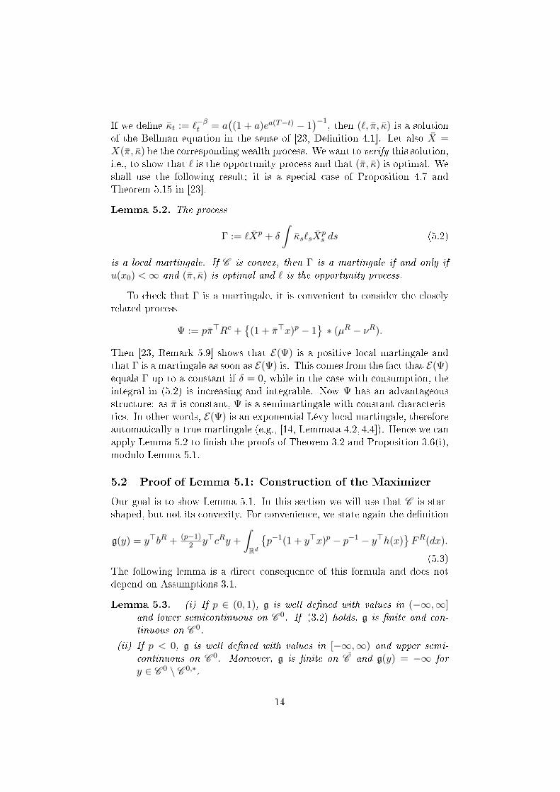
If we de�ne �t := ℓ−�t = a((1 + a)ea(T−t) − 1

)−1, then (ℓ, �, �) is a solutionof the Bellman equation in the sense of [23, De�nition 4.1]. Let also X =X(�, �) be the corresponding wealth process. We want to verify this solution,i.e., to show that ℓ is the opportunity process and that (�, �) is optimal. Weshall use the following result; it is a special case of Proposition 4.7 andTheorem 5.15 in [23].

Lemma 5.2. The process

Γ := ℓXp + �

∫�sℓsX

ps ds (5.2)

is a local martingale. If C is convex, then Γ is a martingale if and only if

u(x0) <∞ and (�, �) is optimal and ℓ is the opportunity process.

To check that Γ is a martingale, it is convenient to consider the closelyrelated process

Ψ := p�⊤Rc +{

(1 + �⊤x)p − 1}∗ (�R − �R).

Then [23, Remark 5.9] shows that ℰ(Ψ) is a positive local martingale andthat Γ is a martingale as soon as ℰ(Ψ) is. This comes from the fact that ℰ(Ψ)equals Γ up to a constant if � = 0, while in the case with consumption, theintegral in (5.2) is increasing and integrable. Now Ψ has an advantageousstructure: as � is constant, Ψ is a semimartingale with constant characteris-tics. In other words, ℰ(Ψ) is an exponential Lévy local martingale, thereforeautomatically a true martingale (e.g., [14, Lemmata 4.2, 4.4]). Hence we canapply Lemma 5.2 to �nish the proofs of Theorem 3.2 and Proposition 3.6(i),modulo Lemma 5.1.

5.2 Proof of Lemma 5.1: Construction of the Maximizer

Our goal is to show Lemma 5.1. In this section we will use that C is star-shaped, but not its convexity. For convenience, we state again the de�nition

g(y) = y⊤bR + (p−1)2 y⊤cRy +

∫ℝd

{p−1(1 + y⊤x)p − p−1 − y⊤ℎ(x)

}FR(dx).

(5.3)The following lemma is a direct consequence of this formula and does notdepend on Assumptions 3.1.

Lemma 5.3. (i) If p ∈ (0, 1), g is well de�ned with values in (−∞,∞]and lower semicontinuous on C 0. If (3.2) holds, g is �nite and con-

tinuous on C 0.

(ii) If p < 0, g is well de�ned with values in [−∞,∞) and upper semi-

continuous on C 0. Moreover, g is �nite on C and g(y) = −∞ for

y ∈ C 0 ∖ C 0,∗.

14

Proof. Fix a sequence yn → y in C 0. A Taylor expansion and (2.1) showthat

∫∣x∣≤"

{p−1(1 + y⊤x)p − p−1 − y⊤ℎ(x)

}FR(dx) is �nite and continuous

along (yn) for " small enough, e.g., " = (2 supn ∣yn∣)−1.If p < 0, we have p−1(1 + y⊤x)p − p−1 − y⊤ℎ(x) ≤ −p−1 − y⊤ℎ(x) and

Fatou's lemma shows that∫∣x∣>"

{p−1(1 + y⊤x)p − p−1 − y⊤ℎ(x)

}FR(dx) is

upper semicontinuous of with respect to y. For p > 0 we have the converseinequality and the same argument yields lower semicontinuity. If p > 0and (3.2) holds, then as the integrand grows at most like ∣x∣p at in�nity, theintegral is �nite and dominated convergence yields continuity.

Let p < 0. For �niteness on C we note that g is even �nite on �C 0 forany � ∈ [0, 1). Indeed, y ∈ �C 0 implies y⊤x ≥ −� > −1 FR(dx)-a.e., hencethe integrand in (5.3) is bounded FR-a.e. and we conclude by (2.1). The lastclaim is immediate from the de�nitions of C 0 and C 0,∗ as well as (5.3).

Assume the version of Lemma 5.1 under Assumptions 3.1(i)-(iii) and (3.2)has already been proved; we argue that the complete claim of that lemmathen follows. Indeed, suppose that Assumptions 3.1(i)-(iv) hold. We �rstobserve that C ∩ C 0,∗ is dense in C ∩ C 0. To see this, note that for y ∈C ∩ C 0 ∖ C 0,∗ and n ∈ ℕ we have yn := (1 − n−1)y → y and yn is in C 0,∗

(by the de�nition) and also in C , due to the star-shape. Using Section 4 andits notation, Assumptions 3.1(i)-(iv) now imply that the transformed model(R, C ) satis�es Assumptions 3.1(i)-(iii) and (3.2). We apply our version ofLemma 5.1 in that model to obtain g∗ := sup

C∩C 0 g < ∞ and a vector� ∈ C ∩ C 0,∗ such that g(�) = g∗. The density of C ∩ C 0,∗ observed aboveand the semicontinuity from Lemma 5.3(i) imply that g∗ := supC∩C 0 g =supC∩C 0,∗ g. Using this argument also for (R, C ), Corollary 4.3(iii) yieldsg∗ = g∗ <∞. Moreover, Corollary 4.3(iv) states that � := Λ⊤� ∈ C ∩ C 0,∗

is a maximizer for g.Summarizing this discussion, it su�ces to prove Lemma 5.1 under As-

sumptions 3.1(i)-(iii) and (3.2); hence these will be our assumptions for therest of the section.

Formally, by di�erentiation under the integral, the directional derivativesof g are given by (y − y)⊤∇g(y) = G(y, y), with

G(y, y) := (y − y)⊤(bR + (p− 1)cRy

)(5.4)

+

∫ℝd

{ (y − y)⊤x

(1 + y⊤x)1−p − (y − y)⊤ℎ(x)}FR(dx).

We take this as the de�nition of G(y, y) whenever the integral makes sense.

Remark 5.4. Formally setting p = 0, we see that G corresponds to the rela-tive rate of return of two portfolios in the theory of log-utility [15, Eq. (3.2)].

Lemma 5.5. Let y ∈ C 0. On the set C 0 ∩ {g > −∞}, G(y, ⋅) is well

de�ned with values in (−∞,∞]. Moreover, G(0, ⋅) is lower semicontinuous

on C 0 ∩ {g > −∞}.

15

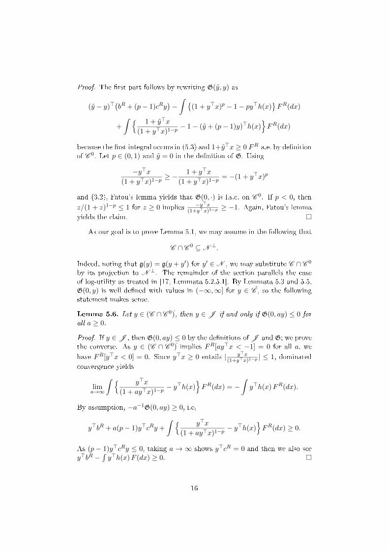
Proof. The �rst part follows by rewriting G(y, y) as

(y − y)⊤(bR + (p− 1)cRy

)−∫ {

(1 + y⊤x)p − 1− py⊤ℎ(x)}FR(dx)

+

∫ { 1 + y⊤x

(1 + y⊤x)1−p − 1− (y + (p− 1)y)⊤ℎ(x)}FR(dx)

because the �rst integral occurs in (5.3) and 1+y⊤x ≥ 0 FR-a.e. by de�nitionof C 0. Let p ∈ (0, 1) and y = 0 in the de�nition of G. Using

−y⊤x(1 + y⊤x)1−p ≥ −

1 + y⊤x

(1 + y⊤x)1−p = −(1 + y⊤x)p

and (3.2), Fatou's lemma yields that G(0, ⋅) is l.s.c. on C 0. If p < 0, thenz/(1 + z)1−p ≤ 1 for z ≥ 0 implies −y⊤x

(1+y⊤x)1−p ≥ −1. Again, Fatou's lemmayields the claim.

As our goal is to prove Lemma 5.1, we may assume in the following that

C ∩ C 0 ⊆ N ⊥.

Indeed, noting that g(y) = g(y + y′) for y′ ∈ N , we may substitute C ∩ C 0

by its projection to N ⊥. The remainder of the section parallels the caseof log-utility as treated in [17, Lemmata 5.2,5.1]. By Lemmata 5.3 and 5.5,G(0, y) is well de�ned with values in (−∞,∞] for y ∈ C , so the followingstatement makes sense.

Lemma 5.6. Let y ∈ (C ∩ C 0), then y ∈J if and only if G(0, ay) ≤ 0 for

all a ≥ 0.

Proof. If y ∈J , then G(0, ay) ≤ 0 by the de�nitions of J and G; we provethe converse. As y ∈ (C ∩ C 0) implies FR[ay⊤x < −1] = 0 for all a, wehave FR[y⊤x < 0] = 0. Since y⊤x ≥ 0 entails ∣ y⊤x

(1+y⊤x)1−p ∣ ≤ 1, dominatedconvergence yields

lima→∞

∫ { y⊤x

(1 + ay⊤x)1−p − y⊤ℎ(x)

}FR(dx) = −

∫y⊤ℎ(x)FR(dx).

By assumption, −a−1G(0, ay) ≥ 0, i.e,

y⊤bR + a(p− 1)y⊤cRy +

∫ { y⊤x

(1 + ay⊤x)1−p − y⊤ℎ(x)

}FR(dx) ≥ 0.

As (p − 1)y⊤cRy ≤ 0, taking a → ∞ shows y⊤cR = 0 and then we also seey⊤bR −

∫y⊤ℎ(x)F (dx) ≥ 0.

16

Proof of Lemma 5.1. Let (yn) ⊂ C ∩ C 0 be such that g(yn)→ g∗. We mayassume g(yn) > −∞ and yn ∈ C 0,∗ by Lemma 5.3, since C 0,∗ ⊆ C 0 is dense.

We claim that (yn) has a bounded subsequence. By way of contradiction,suppose that (yn) is unbounded. Without loss of generality, �n := yn/∣yn∣converges to some �. Moreover, we may assume by rede�ning yn thatg(yn) = max�∈[0,1] g(�yn), because g is continuous on each of the compactsets Cn = {�yn : � ∈ [0, 1]}. Indeed, if p < 0, continuity follows by domi-nated convergence using 1 + �y⊤x ≥ 1 + y⊤x on {x : y⊤x ≤ 0}; while forp ∈ (0, 1), g is continuous by Lemma 5.3.

Using concavity one can check that G(0, a�n) is indeed the directionalderivative of the function g at a�n (cf. [23, Lemma 5.14]). In particular,g(yn) = max�∈[0,1] g(�yn) implies that G(0, a�n) ≤ 0 for a > 0 and all n suchthat ∣yn∣ ≥ a (and hence a�n ∈ Cn). By the star-shape and closedness ofC ∩C 0 we have � ∈ (C ∩C 0). Lemmata 5.3 and 5.5 yield the semicontinuityto pass from G(0, a�n) ≤ 0 to G(0, a�) ≤ 0 and now Lemma 5.6 shows� ∈J , contradicting the NUIPC condition that J ∩ (C ∩ C 0) = ∅.

We have shown that after passing to a subsequence, there exists a limity∗ = limn yn. Lemma 5.3 shows g∗ = limn g(yn) = g(y∗) <∞; and y∗ ∈ C 0,∗

for p < 0. For p ∈ (0, 1), y∗ ∈ C 0,∗ follows as in [23, Lemma A.8].

6 q-Optimal Martingale Measures

In this section we consider � = 0 (no consumption) and C = ℝd. ThenAssumptions 3.1 are equivalent to

NUIPℝd holds and u(x0) <∞ (6.1)

and these conditions are in force for the following discussion. Let M be theset of all equivalent local martingale measures for S = ℰ(R). Then NUIPℝd

is equivalent to M ∕= ∅, more precisely, there exists Q ∈ M under whichR is a Lévy martingale (see [17, Remark 3.8]). In particular, we are in thesetting of Kramkov and Schachermayer [18].

Let q = p/(p − 1) ∈ (−∞, 0) ∪ (0, 1) be the exponent conjugate to p,then Q ∈ M is called q-optimal if E[−q−1(dQ/dP )q] is �nite and minimalover M . If q < 0, i.e., p ∈ (0, 1), then u(x0) < ∞ is equivalent to theexistence of some Q ∈ M such that E[−q−1(dQ/dP )q] < ∞ (cf. Kramkovand Schachermayer [19]).

This minimization problem over M is linked to power utility maximiza-tion by convex duality in the sense of [18]. More precisely, that article con-siders a �dual problem� over an enlarged domain of certain supermartingales.We recall from [24, Proposition 4.2] that the solution to that dual problem isgiven by the positive supermartingale Y = LXp−1, where L is the opportu-nity process and X = x0ℰ(� ∙ R) is the optimal wealth process corresponding

17

to � as in Theorem 3.2. It follows from [18, Theorem 2.2(iv)] that the q-optimal martingale measure Q exists if and only if Y is a martingale, and inthat case Y /Y0 is the P -density process of Q. Recall the functions g and Gfrom (3.1) and (5.4). A direct calculation (or [23, Remark 5.18]) shows

Y /Y0 = ℰ(G(0, �)t+ (p− 1)�⊤Rc +

{(1 + �⊤x)p−1 − 1} ∗ (�R − �R)

).

Here absence of drift is equivalent to G(0, �) = 0, or more explicitly,

�⊤bR + (p− 1)�⊤cR� +

∫ℝd

{ �⊤x

(1 + �⊤x)1−p − �⊤ℎ(x)

}FR(dx) = 0, (6.2)

and in that case

Y /Y0 = ℰ(

(p− 1)�⊤Rc +{

(1 + �⊤x)p−1 − 1}∗ (�R − �R)

). (6.3)

This is an exponential Lévy martingale because � is a constant vector; inparticular, it is indeed a true martingale.

Theorem 6.1. The following are equivalent:

(i) The q-optimal martingale measure Q exists,

(ii) (6.1) and (6.2) hold,

(iii) there exists � ∈ C 0 such that g(�) = maxC 0 g <∞ and (6.2) holds.

Under these equivalent conditions, (6.3) is the P -density process of Q.

Proof. We have just argued the equivalence of (i) and (ii). Under (6.1), thereexists � satisfying (iii) by Theorem 3.2. Conversely, given (iii) we constructthe solution to the utility maximization problem as before and (6.1) follows;recall Remark 3.4(c).

Remark 6.2. (i) If Q exists, (6.3) shows that the change of measure fromP to Q has constant (deterministic and time-independent) Girsanov param-eters

((p− 1)�, (1 + �⊤x)p−1

); compare [12, III.3.24] or Jeanblanc et al. [13,

�A.1, �A.2]. Therefore, R is again a Lévy process under Q. This result waspreviously obtained in [13] by an abstract argument (cf. Section 8 below).

(ii) The existence of Q is a fairly delicate question compared to theexistence of the supermartingale Y . Recalling the de�nition (5.4) of G, (6.2)essentially expresses that the budget constraint C 0 in the maximization ofg is �not binding�. Theorem 6.1 gives an explicit and sharp description forthe existence of Q; this appears to be missing in the previous literature.

7 Extensions to Non-Convex Constraints

In this section we consider the utility maximization problem for some caseswhere the constraints 0 ∈ C ⊆ ℝd are not convex. Let us �rst recapitulate

18

where the convexity assumption was used above. The proof of Lemma 5.1used the star-shape of C , but not convexity. In the rest of Section 5.1, theshape of C was irrelevant except in Lemma 5.2.

We denote by co (C ) the closed convex hull of C .

Corollary 7.1. Let p < 0 and suppose that either (i) or (ii) below hold:

(i) (a) C is star-shaped,

(b) the orthogonal projection of co (C ) ∩ C 0 onto N ⊥ is closed,

(c) NUIPco (C ) holds.

(ii) C ∩ C 0 is compact.

Then the assertion of Theorem 3.2 remains valid.

Proof. (i) The construction of (ℓ, �, �) is as above; we have to substitute theveri�cation step which used Lemma 5.2. The model (R, co (C )) satis�es theassumptions of Theorem 3.2. Hence the corresponding opportunity processLco (C ) is deterministic and bounded away from zero. The de�nition of theopportunity process and the inclusion C ⊆ co (C ) imply that the opportunityprocess L = LC for (R,C ) is also bounded away from zero. Hence ℓ/L isbounded and we can verify (ℓ, �, �) by [23, Corollary 5.4], which makes noassumptions about the shape of C .

(ii) We may assume without loss of generality that C = C ∩ C 0. In (i),the star-shape was used only to construct a maximizer for g. When C ∩C 0 iscompact, its existence is clear by the upper semicontinuity from Lemma 5.3,which also shows that any maximizer is necessarily in C 0,∗. To proceed asin (i), it remains to note that the projection of the compact set co (C ) ∩ C 0

onto N ⊥ is compact, and NUIPco (C ) holds because (co (C )) = {0} sinceco (C ) is bounded.

When the constraints are not star-shaped and p > 0, an additional condi-tion is necessary to ensure that the maximum of g is not attained on C 0∖C 0,∗,or equivalently, to obtain a positive optimal wealth process. In [23, �2.4],the following condition was introduced:

(C3) There exists � ∈ (0, 1) such that y ∈ (C ∩ C 0) ∖ C 0,∗ implies �y ∈ Cfor all � ∈ (�, 1).

This is clearly satis�ed if C is star-shaped or if C 0,∗ = C 0.

Corollary 7.2. Let p ∈ (0, 1) and suppose that either (i) or (ii) below hold:

(i) Assumptions 3.1 hold except that C is star-shaped instead of being con-

vex.

(ii) C ∩ C 0 is compact and satis�es (C3) and u(x0) <∞.

Then the assertion of Theorem 3.2 remains valid.

19

Proof. (i) The assumptions carry over to the transformed model as before,hence again we only need to substitute the veri�cation argument. In view ofp ∈ (0, 1), we can use [23, Theorem 5.2], which makes no assumptions aboutthe shape of C . Note that we have already checked its condition (cf. [23,Remark 5.16]).

(ii) We may again assume C = C ∩C 0 and Remark 4.4 shows that we canchoose C ∩C 0 to be compact in the transformed model satisfying (3.2). Thatis, we can again assume (3.2) without loss of generality. Then g is continuousand hence existence of a maximizer on C ∩ C 0 is clear. Under (C3), anymaximizer is in C 0,∗ by the same argument as in the proof of Lemma 5.1.

The following result covers all closed constraints and applies to most ofthe standard models (cf. Example 2.2).

Corollary 7.3. Let C be closed and assume that C 0 is compact and that

u(x0) <∞. Then the assertion of Theorem 3.2 remains valid.

Proof. Note that (C3) holds for all sets C when C 0,∗ is closed (and henceequal to C 0). It remains to apply part (ii) of the two previous corollaries.

Remark 7.4. (i) For p ∈ (0, 1) we also have the analogue of Proposi-tion 3.6(i): under the assumptions of Corollary 7.2 excluding u(x0) < ∞,(3.2) implies u(x0) <∞.

(ii) The optimal propensity to consume � remains unique even whenthe constraints are not convex (cf. [23, Theorem 3.2]). However, there isno uniqueness for the optimal portfolio. In fact, in the setting of the abovecorollaries, any constant vector � ∈ arg maxC∩C 0 g is an optimal portfolio(by the same proofs); and when C is not convex, the di�erence of two such �need not be in N . See also [23, Remark 3.3] for statements about dynamicportfolios. Conversely, by [23, Theorem 3.2] any optimal portfolio, possiblydynamic, takes values in arg maxC∩C 0 g.

8 Related Literature

We discuss some related literature in a highly selective manner; an exhaustiveoverview is beyond our scope. For the unconstrained utility maximizationproblem with general Lévy processes, Kallsen [14] gave a result of veri�ca-tion type: If there exists a vector � satisfying a certain equation, � is theoptimal portfolio. This equation is essentially our (6.2) and therefore holdsonly if the corresponding dual element Y is the density process of a measure.Muhle-Karbe [22, Example 4.24] showed that this condition fails in a partic-ular model. In the one-dimensional case, he introduced a weaker inequalitycondition [22, Corollary 4.21], but again existence of � was not discussed.(In fact, our proofs show the necessity of that inequality condition; cf. [23,Remark 5.16].)

20

Numerous variants of our utility maximization problem were also studiedalong more traditional lines of dynamic programming. E.g., Benth et al. [2]solve a similar problem with in�nite time horizon when the Lévy processsatis�es additional integrability properties and the portfolios are chosen inthe interval [0, 1]. This part of the literature generally requires technicalconditions, which we sought to avoid.

Jeanblanc et al. [13] study the q-optimal measure Q for Lévy processeswhen q < 0 or q > 1 (note that the considered parameter range does notcoincide with ours). They show that the Lévy structure is preserved under Q,if the latter exists; a result we recovered in Remark 6.2 above for our valuesof q. In [13] this is established by showing that starting from any equivalentchange of measure, a suitable choice of constant Girsanov parameters reducesthe q-divergence of the density. This argument does not seem to extendto our general dual problem which involves supermartingales rather thanmeasures; in particular, it cannot be used to show that the optimal portfoliois a constant vector. A deterministic, but not explicit characterization ofQ is given in [13, Theorem 2.7]. The authors also provide a more explicitcandidate for the q-optimal measure [13, Theorem 2.9], but the condition ofthat theorem fails in general (see Bender and Niethammer [1]).

In the Lévy setting the q-optimal measures (q ∈ ℝ) coincide with the min-imal Hellinger measures and hence the pertinent results apply. See Choulliand Stricker [5] and in particular their general su�cient condition [5, Theo-rem 2.3]. We refer to [13, p. 1623] for a discussion. Our result di�ers in thatboth the existence of Q and its density process are described explicitly interms of the Lévy triplet.

References

[1] C. Bender and C. R. Niethammer. On q-optimal martingale measures inexponential Lévy models. Finance Stoch., 12(3):381�410, 2008.

[2] F. E. Benth, K. H. Karlsen, and K. Reikvam. Optimal portfolio managementrules in a non-Gaussian market with durability and intertemporal substitution.Finance Stoch., 5(4):447�467, 2001.

[3] F. E. Benth, K. H. Karlsen, and K. Reikvam. Optimal portfolio selectionwith consumption and nonlinear integro-di�erential equations with gradientconstraint: a viscosity solution approach. Finance Stoch., 5(3):275�303, 2001.

[4] S. Cawston and L. Vostrikova. Minimal f -divergence martingale measures andoptimal portfolios for exponential Lévy models with a change-point. PreprintarXiv:1004.3525v1, 2010.

[5] T. Choulli and C. Stricker. Comparing the minimal Hellinger martingale mea-sure of order q to the q-optimal martingale measure. Stochastic Process. Appl.,119(4):1368�1385, 2009.

[6] C. Czichowsky and M. Schweizer. Closedness in the semimartingale topologyfor spaces of stochastic integrals with constrained integrands. To appear inSém. Probab., 2009.

21

[7] C. Czichowsky, N. Westray, and H. Zheng. Convergence in the semimartingaletopology and constrained portfolios. To appear in Sém. Probab., 2008.

[8] L. Foldes. Conditions for optimality in the in�nite-horizon portfolio-cum-saving problem with semimartingale investments. Stochastics Stochastics Rep.,29(1):133�170, 1990.

[9] N. C. Framstad, B. Øksendal, and A. Sulem. Optimal consumption and port-folio in a jump di�usion market. Discussion Paper, Norwegian School of Eco-

nomics and Business Administration, 1999.[10] P. Grandits. On martingale measures for stochastic processes with independent

increments. Theory Probab. Appl., 44(1):39�50, 2000.[11] J. M. Harrison and S. R. Pliska. Martingales and stochastic integrals in the

theory of continuous trading. Stochastic Process. Appl., 11(3):215�260, 1981.[12] J. Jacod and A. N. Shiryaev. Limit Theorems for Stochastic Processes.

Springer, Berlin, 2nd edition, 2003.[13] M. Jeanblanc, S. Klöppel, and Y. Miyahara. Minimal fq-martingale measures

for exponential Lévy processes. Ann. Appl. Probab., 17(5/6):1615�1638, 2007.[14] J. Kallsen. Optimal portfolios for exponential Lévy processes. Math. Methods

Oper. Res., 51(3):357�374, 2000.[15] I. Karatzas and C. Kardaras. The numéraire portfolio in semimartingale �-

nancial models. Finance Stoch., 11(4):447�493, 2007.[16] I. Karatzas and G. �itkovi¢. Optimal consumption from investment and

random endowment in incomplete semimartingale markets. Ann. Probab.,31(4):1821�1858, 2003.

[17] C. Kardaras. No-free-lunch equivalences for exponential Lévy models underconvex constraints on investment. Math. Finance, 19(2):161�187, 2009.

[18] D. Kramkov and W. Schachermayer. The asymptotic elasticity of utility func-tions and optimal investment in incomplete markets. Ann. Appl. Probab.,9(3):904�950, 1999.

[19] D. Kramkov and W. Schachermayer. Necessary and su�cient conditions in theproblem of optimal investment in incomplete markets. Ann. Appl. Probab.,13(4):1504�1516, 2003.

[20] R. C. Merton. Lifetime portfolio selection under uncertainty: the continuous-time case. Rev. Econom. Statist., 51:247�257, 1969.

[21] J. Mossin. Optimal multiperiod portfolio policies. J. Bus., 41(2):215�229,1968.

[22] J. Muhle-Karbe. On Utility-Based Investment, Pricing and Hedging in Incom-

plete Markets. PhD thesis, TU München, 2009.[23] M. Nutz. The Bellman equation for power utility maximization with semi-

martingales. Preprint arXiv:0912.1883v1, 2009.[24] M. Nutz. The opportunity process for optimal consumption and investment

with power utility. To appear in Math. Financ. Econ., 2009.[25] P. A. Samuelson. Lifetime portfolio selection by dynamic stochastic program-

ming. Rev. Econ. Statist., 51(3):239�246, 1969.[26] K.-I. Sato. Lévy Processes and In�nitely Divisible Distributions. Cambridge

University Press, Cambridge, 1999.[27] W. Schoutens. Lévy Processes in Finance: Pricing Financial Derivatives.

Wiley, Chichester, 2003.

22