ARTICLE IN PRESS

OpticsOptikOptikOptik 120 (2009) 242–246

0030-4026/$ - se

doi:10.1016/j.ijl

�CorrespondE-mail addr

www.elsevier.de/ijleo

Power transfer characteristics among N parallel single-mode optical fibers

Ye Wang, Dajian Xue, Xuanhui Lu�

State Key Laboratory of Modern Optical Instrumentation, Department of Physics, Optics Institute, Zhejiang University,

Hangzhou 310027, PR China

Received 4 September 2006; accepted 6 May 2007

Abstract

Based on the coupled-mode theory, the power transfer among ‘‘- - - -’’ arranged parallel single-mode optical fibershas been investigated. The analysis shows that the distances between each two of the N fiber centers have effects on thecoupling coefficient and power transfer. The solution of the coupled-equations for three parallel single-mode opticalfibers is given, and is studied for different initial conditions comparatively. Numerical simulations show that powertransfer will be periodical during coupling among parallel single-mode optical fibers. These results can be extended tomulti-parallel single-mode optical fibers.r 2007 Elsevier GmbH. All rights reserved.

Keywords: Optical fiber array; Modes coupling; Power transfer

1. Introduction

It is a well-known fact that if the optical fiber coresare brought close enough to each other, wave couplingand power transfer among optical fibers happen due tothe interaction of the extended evanescent optical fieldsright outside the cores. The coupling is important todivide and mix optical signals for various optical fibercomponents, such as fiber couplers [1,2] and powerdividers [3]. For example, the well-known phenomenonof evanescent wave coupling has wide applications suchas the design of waveguide switches [4], an importantpassive device in optical communications. However, insome other cases, an avoidance of wave coupling effectsamong ‘‘- - -’’ arranged optical fibers is needed. Arepresentative example is pivotal components in a newscanning system for imaging.

e front matter r 2007 Elsevier GmbH. All rights reserved.

eo.2007.05.012

ing author. Tel./fax: +86571 87953232.

ess: xhlu@zju.edu.cn (X. Lu).

In previous studies, Snyder [5] presented a generalcoupled-mode theory and obtained conclusive resultsthat could be used in a number of different wavepropagation problems. In his study, the solution of thecoupled-equations for two parallel optical fibers wasfurther presented. He also studied the coupling effectson the situation of a special fiber surrounded by other N

identical fibers. However, it is only a special case amongthe generic two-body coupling problems. McIntyre andSnyder [6] extended Snyder’s results to the coupling ofmulti-mode fibers, and discussed the power transferbetween a special fiber and six other non-identical fibers,which is also a generic two-mode coupling problem.Chang, Huang, and Wu [7] analyzed numerically thecases of power transfer between a signal-mode fiber anda multi-mode fiber. In general cases, two-mode couplingof many ‘‘- - -’’ arranged parallel optical fibers cannot beeasily solved. To determine the details of the powertransfer among the ‘‘- - -’’ arranged N fibers, it isrequired to solve the equations for N systems. In thispaper, we derived the solution of the coupled-equations

ARTICLE IN PRESSY. Wang et al. / Optik 120 (2009) 242–246 243

of three parallel single-mode (SM) optical fibers. Thesolution can be extended to N parallel SM optical fibers.

2. The coupled-mode method

We consider N infinitely long and parallel identicalcores embedded in the cladding background, as shownin Fig. 1. The refractive index of the SM core and thecladding are denoted as n1 and n2, respectively. Theradius of the SM core and the distance between twocenters of the neighboring cores are shown as r and d,respectively.

We adopt the coupled-mode equations derived inRef. [5], in which only the closest coupling is taken intoaccount. For the present system of N(N43) parallelfibers of no loss, the equations are as follows:

dA1ðzÞ

dzþ ib1A1ðzÞ ¼ �iA2ðzÞC12, (1)

dAmðzÞ

dzþ ibmAmðzÞ ¼ �iAm�1ðzÞCmðm�1Þ � iAmþ1ðzÞCmðmþ1Þ

ðm ¼ 2; 3; . . . ;N � 1Þ, ð2Þ

dANðzÞ

dzþ ibNAN ðzÞ ¼ �iAN�1ðzÞCNðN�1Þ. (3)

The z-axis in Cartesian coordinates is taken to beparallel to the fiber axes. In Eqs. (1)–(3), the subscriptsm and N refer to the mth fiber and Nth fiber,respectively. b represents the propagation constant ofmode, and A(z) represents the coefficient of mode onz ¼ constant. The symbol Cab is the coupling coefficientbetween the ath and the bth fibers, and is defined as

Cab ¼o2

ZAb

ðn21 � n2

2Þ e*

a � e*

b ds, (4)

where o is the wave frequency, Ab represents the crosssection of the bth cores, e

*is the electric field vector of

mode. All modes are assumed to travel in the positive z

direction. All the propagation constants of mode areequal because the N SM fibers are identical, and allcoupling coefficients are equal as well according toEq. (4). Thus all the propagation constants of mode and

......

dd

n1n1 n1

n2 z

1 2 3 Nρ ρ

Fig. 1. N parallel single-mode optical fibers system.

all coupling coefficients can be shown as b and C,respectively. It has been shown that the power transferbetween the forward and backward modes is very smalland can be neglected for the case where the couplingcoefficients are much smaller than the propagationconstants of mode, i.e., the case satisfying the weak-coupling condition [5]. In the following examples, C isfound to be much smaller than the accompanying valueb. Thus, we only consider weak-coupling cases.

b and C were given [5,6] in the following formsby introducing three dimensionless parameters U, V

and W:

b ¼2pn1

l

� �2

�U2

r2

" #1=2, (5)

C ¼

ffiffiffidp

U2K0½W ðd=rÞ�rV 3K2

1ðW Þ, (6)

where l is the wavelength of light in a vacuum, K’s aremodified Hankel functions, and d is defined as

d ¼ 1�n2

n1

� �2

. (7)

A dimensionless frequency V is defined to be

V ¼2prn1

ffiffiffidp

l¼ U2 þW 2. (8)

U is given approximately as

U ffi 2:405 e�ð1�d=2ÞV . (9)

3. Results and discussion

3.1. Solutions for two different initial conditions and

discussion

When N ¼ 3, the solutions to Eqs. (1)–(3) are given as

A1ðzÞ

A2ðzÞ

A3ðzÞ

0BB@

1CCA ¼ q1

1

0

�1

0BB@

1CCAe�ibz þ q2

1ffiffiffi2p

1

0BB@

1CCAe�iðbþ

ffiffi2p

CÞz

þ q3

1

�ffiffiffi2p

1

0BB@

1CCAe�iðb�

ffiffi2p

CÞz, ð10Þ

where q1, q2, q3, are determined by initial conditions.Two cases of unit power coupling are considered.

1.

Excitation of the 1st fiber with unit power A1ð0Þ ¼ 1with A2ð0Þ ¼ 0, A3ð0Þ ¼ 0: By combining this condi-tion with Eq. (10), we obtain q1 ¼ 1=2, q2 ¼ q3 ¼

1=4. The power of each fiber can be shown as PiðzÞ ¼

jAiðzÞj2 (i ¼ 1, 2, 3). If l ¼ 1.31 mm, the refractive

ARTICLE IN PRESS

Fig

op

wit

Cu

res

po

Y. Wang et al. / Optik 120 (2009) 242–246244

index of the core is n1 ¼ 1.458, the refractive index ofthe cladding is n2 ¼ 1.455, and the radiuses of thecores are r ¼ 4 mm. The results of the power couplingamong the three fibers are shown in Fig. 2 for d ¼ 12,20, and 50 mm, respectively. In all three cases, thethree fibers appear to undergo significant powercoupling and variations, as indicated by the power vs.distance curves shown in the figures. It is noticed in

0 10

0.4

POW

ER

1

2

3

0 50 75 100

1.0

POW

ER

1

2

3

0 600 800 1000

POW

ER

1

2

3

1.0

0.8

0.6

0.2

0.0

DISTANCE z / mm

DISTANCE z / mm

2 4 6 8

0.8

0.6

0.4

0.2

0.0

25 125

DISTANCE z / m

1.0

0.8

0.6

0.4

0.2

0.0

200 400 1200

(a)

(b)

(c)

. 2. Power variations versus propagation distance of three

tical fibers according to the initial condition 1. Three cases

h N ¼ 3, d ¼ 12, 20, and 50mm, respectively, are shown.

rves 1–3 represent the power variations of optical fibers 1–3,

pectively. The unit power is defined as the original value of

wer when Z ¼ 0, and it is the same as below.

Fig. 2(a) that at the distance of 4.48mm, almost allthe power of the 1st fiber has been transferred to thatof the 3rd one. In the cases of Fig. 2(b) and (c), thepower of the 1st fiber drops to zero at z ¼ 56.5mmand 482.8m, respectively, and the power of the 3rdfiber reaches the peak of unit power simultaneously.At the beginning of the propagation, the distance atwhich the power of the 1st fiber drops to half of itsinitial value is found to be 1.63mm for the case ofd ¼ 12 mm. And as the coupling strength decreasesfor the case of d ¼ 50 mm, the distance increasesmonotonously to 175.5m. Initially, the power of the2nd fiber is observed to gain most of its power fromthe 1st fiber in all three cases. The maximum powerpoint of the 2nd fiber depends on the couplingstrength and the spacing between the two fibers, andreaches half of the maximum power value of the 1stand the 3rd fibers in all three cases. It is found thatthe power of the 2nd fiber decreases to zero at nearlythe same position as that of the 1st fiber. Aspropagation distance goes on, the power of the 1stfiber begins to increase while the power of the 3rd onedecreases. The power of the 2nd fiber goes up initiallyand then drops. Fig. 2(a) shows that the powers of the2nd and the 3rd fibers drops to zero and the power ofthe 1st fiber returns to unit power at the distance of8.965mm at d ¼ 12 mm. The cases of d ¼ 20 and50 mm show the same variation trend of power. Allthree fibers have the periodical power transfer alongthe propagation distance.

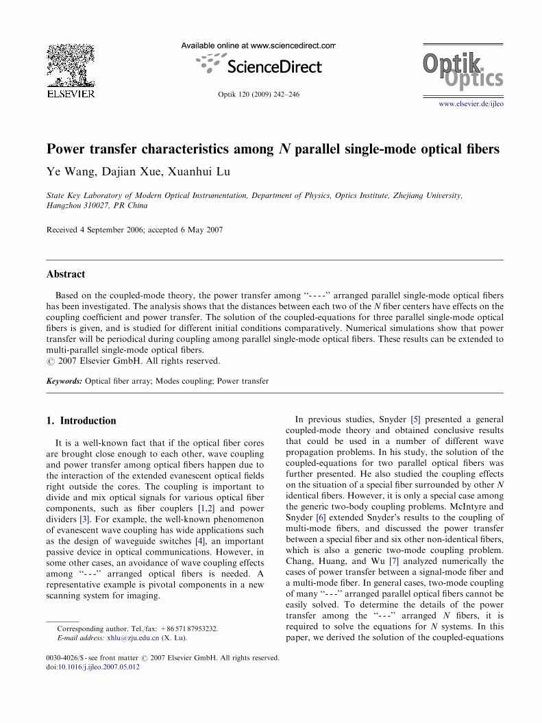
It can be seen by analyzing Fig. 2(a)–(c) that thecoupling period increases as the space d increases.The cause is that the coupling coefficient goes downobservably with the increasing space between the twoneighboring fibers, and the coupling strength amongoptical fibers falls dramatically accordingly. Thus, theoutward transfer velocity of the power of the 1st fiberdecreases too. So the wave propagation distance islonger as the initial power of the 1st power drops tozero. Fig. 3 shows the relationship between thecoupling coefficient and the space between the twoneighboring fibers. When d432 mm (correspondinglyC ¼ 0.999), the coupling is so weak that it can beneglected in this case.

2.

Excitation of the 2nd fiber with unity power A2ð0Þ ¼ 1with A1ð0Þ ¼ 0, A3ð0Þ ¼ 0: The power coupling ofanother case is presented in Fig. 4. Now the initialcondition is A2ð0Þ ¼ 1, A1ð0Þ ¼ 0, and A3ð0Þ ¼ 0.Using Eq. (10), we have q1 ¼ 0, q2 ¼

ffiffiffi2p �

4, q3 ¼

�ffiffiffi2p �

4, for d ¼ 20 mm. It is observed that thevariations are similar to those shown in Fig. 2(b).However, the power transfer of the 1st and the 3rdfibers is synchronous and their transfer velocities arealso same. The maximal power of the 1st fiber and the3rd fiber reaches half of the total power. Figs. 4 and2(b) show that the power transfer velocities of the 1st

ARTICLE IN PRESS

0 15 30 45 60 75

1.0

POW

ER

1

2

30.8

0.6

0.4

0.2

0.0

DISTANCE z / mm

Fig. 4. Power variations versus propagation distance accord-

ing to the initial conditions 2 when N ¼ 3, d ¼ 20 mm. Now

curves 1 and 3 are overlapping.

0 30 60 90 120

0.0

0.6

POW

ER

1

2

3

4

1.0

0.8

0.4

0.2

DISTANCE z / mm

1

150

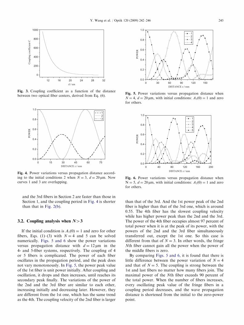
Fig. 5. Power variations versus propagation distance when

N ¼ 4, d ¼ 20mm, with initial conditions: A1ð0Þ ¼ 1 and zero

for others.

12 16 28 32

0

200

400

600

800

1000C

oupl

ing

coef

fici

ent C

d / um

20 24

Fig. 3. Coupling coefficient as a function of the distance

between two optical fiber centers, derived from Eq. (6).

0 40 80 120 160

POW

ER

1

2

3

4

5

DISTANCE z / mm

200

1.0

0.8

0.6

0.4

0.2

0.0

Fig. 6. Power variations versus propagation distance when

N ¼ 5, d ¼ 20 mm, with initial conditions: A1ð0Þ ¼ 1 and zero

for others.

Y. Wang et al. / Optik 120 (2009) 242–246 245

and the 3rd fibers in Section 2 are faster than those inSection 1, and the coupling period in Fig. 4 is shorterthan that in Fig. 2(b).

3.2. Coupling analysis when N43

If the initial condition is A1ð0Þ ¼ 1 and zero for otherfibers, Eqs. (1)–(3) with N ¼ 4 and 5 can be solvednumerically. Figs. 5 and 6 show the power variationsversus propagation distance with d ¼ 12 mm in the4- and 5-fiber systems, respectively. The coupling of 4or 5 fibers is complicated. The power of each fiberoscillates in the propagation period, and the peak doesnot vary monotonously. In Fig. 5, the power peak valueof the 1st fiber is unit power initially. After coupling andoscillation, it drops and then increases, until reaches itssecondary peak finally. The variations of the power ofthe 2nd and the 3rd fiber are similar to each other,increasing initially and decreasing later. However, theyare different from the 1st one, which has the same trendas the 4th. The coupling velocity of the 2nd fiber is larger

than that of the 3rd. And the 1st power peak of the 2ndfiber is higher than that of the 3rd one, which is around0.55. The 4th fiber has the slowest coupling velocitywhile has higher power peak than the 2nd and the 3rd.The power of the 4th fiber occupies almost 97 percent oftotal power when it is at the peak of its power, with thepowers of the 2nd and the 3rd fiber simultaneouslytransferred out, except the 1st one. So this case isdifferent from that of N ¼ 3. In other words, the fringeNth fiber cannot gain all the power when the power ofthe middle fibers is zero.

By comparing Figs. 5 and 6, it is found that there islittle difference between the power variation of N ¼ 4and that of N ¼ 5. The coupling is strong between the1st and last fibers no matter how many fibers join. Themaximal power of the Nth fiber exceeds 90 percent ofthe total power. When the number of fibers increases,every oscillating peak value of the fringe fibers in acoupling period decreases, and the wave propagationdistance is shortened from the initial to the zero-powerpoint.

ARTICLE IN PRESSY. Wang et al. / Optik 120 (2009) 242–246246

4. Conclusion

In this paper, we have calculated the power transferamong many ‘‘- - -’’ arranged parallel SM optical fibersbased on a coupled-mode analysis. Different initialcoupling conditions and different numbers of opticalfibers are studied comparatively. Numerical simulationsand theoretical curves show that the power transfervaries regularly among N ‘‘- - -’’ arranged parallel SMoptical fibers. The coupling becomes stronger when thespace between the two neighboring fibers is smaller.When using N ‘‘- - -’’ arranged parallel optical fibers, thepower coupling can be controlled in different applica-tions if the space between two neighboring fibers and thepropagation distance are adjusted properly. On theother hand, after investigating these results, the couplingcan be avoided efficiently in the scan imaging system,where it is necessary to keep uniformity for every spot.

Acknowledgments

This work is supported by National Science Founda-tion of China (Grant no. 10334050) and ScientificProject of Zhejiang Province (Grant no. 2005c21003).

References

[1] G.J. Liu, B.M. Liang, G.L. Jin, et al., Switching

characteristics of variable coupling coefficient nonlinear

directional coupler, J. Lightwave Technol. 22 (6) (2004)

1591–1597.

[2] J.S. Li, Z.W. Bao, The neural network model of optical

fiber direction coupler, in: IEEE International Conference

on Neural Networks & Singal Processing, Nanjing, China,

December 14–17, 2003.

[3] J. Hudgings, L. Molter, M. Dutta, Design and modeling of

passive optical switches and power dividers using non-

planar coupled fiber arrays, IEEE J. Quantum Electron. 36

(12) (2000) 1438–1444.

[4] L.A. Molter-Orr, H.A. Haus, N�N coupled waveguide

switch, Opt. Lett. 9 (10) (1984) 466–467.

[5] A.W. Snyder, Coupled-mode theory for optical fibers,

J. Opt. Soc. Am. 62 (11) (1972) 1267–1277.

[6] P.D. McIntyre, A.W. Snyder, Power transfer between

optical fibers, J. Opt. Soc. Am. 63 (12) (1973) 1518–1527.

[7] H.C. Chang, H.S. Huang, J.S. Wu, Wave coupling between

parallel single-mode and multimode optical fibers, IEEE

Trans. Microwave Theory Tech. 34 (12) (1986) 1337–1343.