Power Tracing in a Deregulated Power System : IEEE 14-Bus … · Power Tracing in a Deregulated...

Power Tracing in a Deregulated Power System : IEEE 14-Bus Case

Satyavir Singh

Indian Institute of Technology, Rookee,India

E-mail: [email protected]

Abstract

In this present era , a fair transmission pricing scheme is

an important issue due to incresed deregulation and

restructuring of power sector. In this view, issue of

tracing the flow of electricity has been gain importance

as its solution helps in evaluating a fair and transparent

tariff.An electricity tracing method would make it

possible to charge the generators and/or consumers on

the basis of actual transmission facility used. This paper

focuses on tracing of electricity using Bialek’s tracing

algorithm .Case study is carried out using an IEEE 14-

bus system with three simultaneous bilateral transactions

simulated in Power world simulator.

1. Introduction

Power system operation in many electricity supply

systems worldwide, has been experiencing dramatic

changes due to the on going restructuring of the industry.

The vertically integrated structure of power industry is

being replaced by market structure which led to a

significant increase in power wheeling transactions. In

such a structure a transmission system is being used by

multiple generation and load entities that do not own the

transmission system. In view of market operation it

becomes more important to know the role of individual

generators and loads to transmission lines and power

transfer between individual generators to loads. Basically

there are three methods for power tracing which are

described below [1]:

1.1. Node method

In a meshed transmission network there are number of

possible routes by which electrical power can flow from

sources to sinks. It is possible to determine relation

between the generators/loads and the flows in

transmission lines by means of sensitivity analysis, that is

by determining how a change in nodal

generation/demand influences the flow in a particular line

[2, 3]. Although this method based on dc load flow and

sensitivity analysis cannot consider accurately, the

reactive power transfer allocation and system non

linearity. A novel electricity tracing method has been

proposed [4] which, under the assumption that nodal

inflows are shared proportionally between the nodal

outflows, allows one to trace the flow of electricity in a

meshed network. This method was proposed by J.Bialek

[5] .The complete description of this method for the

tracing of real power is given in section 2.

The characteristics of nodal method are given below:

(i) The transmission losses must be removed from the

lines before the application of the method.

(ii) Matrix calculation is more complex and the speed is a

problem for a big network.

(iii) The method can handle cyclic flows in the system, so

the method is suitable for systems with loop flows.

(iv) If MVAR tracing is required, the method becomes

messy with the introduction of artificial nodes.

In [6] a new method for determining the generator’s

contribution to a particular load is presented. The method

uses the nodal generation distribution factors (NGDF-s).

It features a search algorithm, capable of handling the

active and reactive powers. Paper [7] provides new

insights into the electricity tracing methodology, by

representing the inverted tracing upstream and

downstream distribution matrices in the form of matrix

power series and by applying linear algebra analysis. A

rigorous mathematical proof of the invertibility of the

tracing distribution matrices is given, along with a proof

of convergence for the matrix power series

1.2. Graph method

This method assumes that a generator has the priority to

provide power to the load on the same bus and is based

on the following lemmas of graph theory [8].

Lemma 1: A lossless, finite-nodes power system without

loop flow has at least one pure source, i.e. a generator bus

with all incident lines carrying outflows.

Lemma 2: A lossless, finite-nodes power system without

Satyavir Singh et al ,Int.J.Computer Technology & Applications,Vol 3 (3), 887-894

IJCTA | MAY-JUNE 2012 Available [email protected]

887

ISSSN:2229-6093

loop flow has at least one pure sink, i.e. a load bus with

all incident lines carrying inflows. The characteristics of

the graph method are:

(i) The transmission losses must be removed from the

lines before the application of the method.

(ii) Extraction factor, Contribution factor matrices are

sparse and easy to calculate.

(iii) The method cannot handle loop flows, but is able to

detect loop flows.

(iv) A generator has the priority to provide power to the

load on the same bus

1.3. Method of commons

This method was proposed by Kirschen and additional

details of the method can be found in [8, 9]. The

technique can be applied to both active and reactive

power. The principal ideas of the method are presented

below.

(i) The transmission losses can be directly accounted for

and the contributions to them calculated.

(ii) The contribution factors to all the loads inside a

Common as well as the outflows are constant.

(iii) More simple and intuitive for large systems.

(iv) The size and shape of a Common is subjected to

change radically even with a small change in the

direction of line flows.

2. Proportional sharing principle

The proportional sharing principle is based on kirchhoff’s

current law and is topological in nature. It deals with a

general transportation problem and assumes that the

network node is a perfect mixer of incoming flows.

Practically the only requirement for the input data is that

Kirchhoff’s current law must be satisfied for all the nodes

in the network.In this respect the method is equally

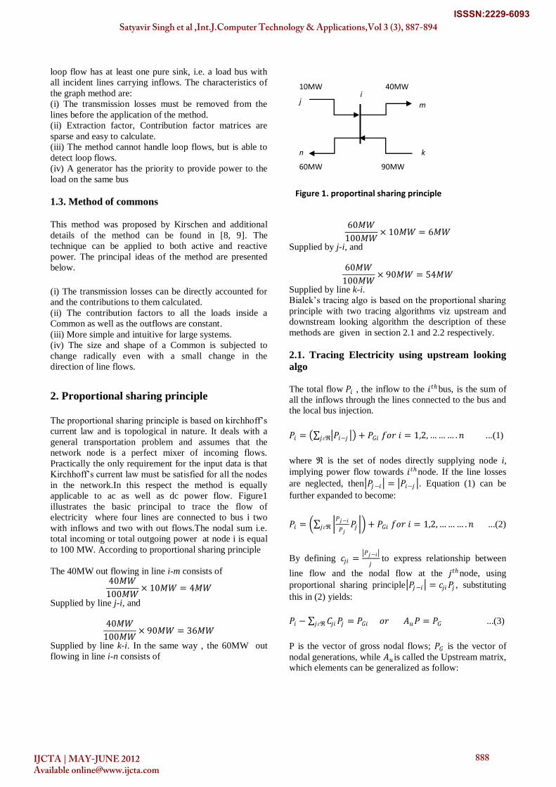
applicable to ac as well as dc power flow. Figure1

illustrates the basic principal to trace the flow of

electricity where four lines are connected to bus i two

with inflows and two with out flows.The nodal sum i.e.

total incoming or total outgoing power at node i is equal

to 100 MW. According to proportional sharing principle

The 40MW out flowing in line i-m consists of 40𝑀𝑊

100𝑀𝑊× 10𝑀𝑊 = 4𝑀𝑊

Supplied by line j-i, and

40𝑀𝑊

100𝑀𝑊× 90𝑀𝑊 = 36𝑀𝑊

Supplied by line k-i. In the same way , the 60MW out

flowing in line i-n consists of

Figure 1. proportinal sharing principle

60𝑀𝑊

100𝑀𝑊× 10𝑀𝑊 = 6𝑀𝑊

Supplied by j-i, and

60𝑀𝑊

100𝑀𝑊× 90𝑀𝑊 = 54𝑀𝑊

Supplied by line k-i.

Bialek’s tracing algo is based on the proportional sharing

principle with two tracing algorithms viz upstream and

downstream looking algorithm the description of these

methods are given in section 2.1 and 2.2 respectively.

2.1. Tracing Electricity using upstream looking

algo

The total flow 𝑃𝑖 , the inflow to the 𝑖𝑡ℎbus, is the sum of

all the inflows through the lines connected to the bus and

the local bus injection.

𝑃𝑖 = 𝑃𝑖−𝑗 𝑗ɛℜ + 𝑃𝐺𝑖 𝑓𝑜𝑟 𝑖 = 1,2, … … … . 𝑛 ...(1)

where ℜ is the set of nodes directly supplying node i,

implying power flow towards 𝑖𝑡ℎnode. If the line losses

are neglected, then 𝑃𝑗−𝑖 = 𝑃𝑖−𝑗 . Equation (1) can be

further expanded to become:

𝑃𝑖 = 𝑃𝑗−𝑖

𝑃𝑗𝑃𝑗 𝑗ɛℜ + 𝑃𝐺𝑖 𝑓𝑜𝑟 𝑖 = 1,2, … … … . 𝑛 ...(2)

By defining 𝑐𝑗𝑖 = 𝑃𝑗−𝑖

𝑗 to express relationship between

line flow and the nodal flow at the 𝑗𝑡ℎnode, using

proportional sharing principle 𝑃𝑗−𝑖 = 𝑐𝑗𝑖 𝑃𝑗 , substituting

this in (2) yields:

𝑃𝑖 − 𝐶𝑗𝑖 𝑃𝑗𝑗ɛℜ = 𝑃𝐺𝑖 𝑜𝑟 𝐴𝑢𝑃 = 𝑃𝐺 ...(3)

P is the vector of gross nodal flows; 𝑃𝐺 is the vector of

nodal generations, while 𝐴𝑢 is called the Upstream matrix,

which elements can be generalized as follow:

10MW

90MW

40MW

60MW

i j

k

m

n



888

ISSSN:2229-6093

𝐴𝑢 𝑖𝑗 =

1 𝑓𝑜𝑟 𝑖 = 𝑗

−𝐶𝑗𝑖 = − 𝑃𝑗−𝑖

𝑃𝑗 𝑓𝑜𝑟 𝑗ɛℜ

0 𝑜𝑡ℎ𝑒𝑟𝑤𝑖𝑠𝑒

...(4)

The 𝑖𝑡ℎelement of 𝑃 = 𝐴𝑢−1𝑃𝐺 shows the participation

of the 𝑘𝑡ℎgeneration to the 𝑖𝑡ℎnodal flow and determines

the relative participation of the nodal generations in

meeting a retailer’s demand, given as:

𝑃𝑖 = 𝐴𝑢−1

𝑖𝑘𝑛𝑘=1 𝑃𝐺𝑘 𝑓𝑜𝑟 𝑖 = 1,2, … …… . 𝑛 ...(5)

A line out flow in line j-i from node i can be therefore

calculated using proportional sharing principle ,as

𝑃𝑗−𝑖 =𝑃𝑗−𝑖

𝑃𝑖 𝐴𝑢

−1 𝑖𝑘

𝑛𝑘=1 𝑃𝐺𝑘 𝑓𝑜𝑟 𝑖 = 1,2, … . 𝑛 ...(6)

Finally, load demand at the 𝑖𝑡ℎ bus, applying the

proportional methodology is given by:

𝑃𝐿𝑖 =𝑃𝐿𝑖

𝑃𝑖𝑃𝑖

𝑃𝐿𝑖 =𝑃𝐿𝑖

𝑃𝑖 𝐴𝑢

−1 𝑖𝑘

𝑛𝑘=1 𝑃𝐺𝑘 𝑓𝑜𝑟 𝑖 = 1,2, … … . 𝑛 ...(7)

This equation shows the contribution of the 𝑖𝑡ℎsystem

generator to the 𝑘𝑡ℎ load demand and can be used to trace

where the power of a particular load comes from.

2.2. Tracing Electricity using downstream

looking algo

The total flow 𝑃𝑖 , the outflow to the 𝑖𝑡ℎbus, is the sum of

all the outflows through the lines connected to the bus

and the local bus load

𝑃𝑖 = 𝑃𝑖−𝑙 𝑙ɛ𝜇 + 𝑃𝐿𝑖 𝑓𝑜𝑟 𝑖 = 1,2, … … … . 𝑛 ...(8)

where μ is the set of nodes directly supplied from node i,

implying power flowing from the 𝑖𝑡ℎnode. If the line

losses are neglected, then 𝑃𝑙−𝑖 = 𝑃𝑖−𝑙 .Equation (8) can

be further expanded into:

𝑃𝑖 = 𝑃𝑙−𝑖

𝑃𝑙𝑃𝑙 𝐿ɛ𝜇 + 𝑃𝐿𝑖 𝑓𝑜𝑟 𝑖 = 1,2, … … … . 𝑛 ...(9)

Defining 𝑐𝑙𝑖 = 𝑃𝑙−𝑖

𝑃𝑙 expressing relationship between line

flow and the nodal flow at the 𝑙𝑡ℎ node and using

proportional sharing principle, 𝑃𝑙−𝑖 = 𝑐𝑙𝑖𝑃𝑙 . Substituting

this in (9) yields

𝑃𝑖 − 𝐶𝑙𝑖𝑃𝑙𝑙ɛ𝜇 = 𝑃𝐿𝑖 𝑜𝑟 𝐴𝑑𝑃 = 𝑃𝐿 ...(10)

𝑃 is the vector of net nodal powers; 𝑃𝐿is the vector of

nodal load demands, while 𝐴𝑑 is called the Downstream

matrix, which elements can be generalized as follow:

𝐴𝑑 𝑖𝑙 =

1 𝑓𝑜𝑟 𝑖 = 𝑙

−𝐶𝑙𝑖 = − 𝑃𝑙−𝑖

𝑃𝑙 𝑓𝑜𝑟 𝑙ɛ𝜇

0 𝑜𝑡ℎ𝑒𝑟𝑤𝑖𝑠𝑒

...(11)

The 𝑖𝑡ℎelement of 𝑃 = 𝐴𝑑−1𝑃𝐿 shows the distribution of

the 𝑖𝑡ℎnodal power between all the loads in the system.

In summation form,

𝑃𝑖 = 𝐴𝑑−1

𝑖𝑘𝑛𝑘=1 𝑃𝐿𝑘 𝑓𝑜𝑟 𝑖 = 1,2, … … … . 𝑛 ...(12)

The inflow to node i from line i-l can be calculated using

the proportional sharing principle as

𝑃𝑖−𝑙 =𝑃𝑖−𝑙

𝑃𝑖 𝐴𝐷

−1 𝑖𝑘

𝑛𝑘=1 𝑃𝐿𝑘 𝑓𝑜𝑟 𝑖 = 1,2, … . 𝑛 ...(13)

this equation allows to determine how the line flows

supply individual loads.

The generation at a node is also an inflow and can be

calculated using the proportional sharing principle as

𝑃𝐺𝑖 =𝑃𝐺𝑖

𝑃𝑖𝑃𝑖

𝑃𝐺𝑖 =𝑃𝐺𝑖

𝑃𝑖 𝐴𝑑

−1 𝑖𝑘

𝑛𝑘=1 𝑃𝐿𝑘 𝑓𝑜𝑟 𝑖 = 1,2, … … . 𝑛 ...(14)

This equation again shows that the share of the output of

the 𝑖𝑡ℎ generator used to supply the 𝑘𝑡ℎ load demand. The

results obtained in case of equation (7) and equation (14)

are same i.e in case of equation (14) a transpose of table 2

results.

3. Results and discussion

IEEE 14-bus system is simulated in power world

simulator with additional three bilateral transactions

which involve different transaction locations. The detail

of the transactions are as follows:

T1: Injection of 20 MW at bus1 and removal at bus 5;



The transmission network data and load flow results are

given in table 4-7. The proportional sharing



889

ISSSN:2229-6093

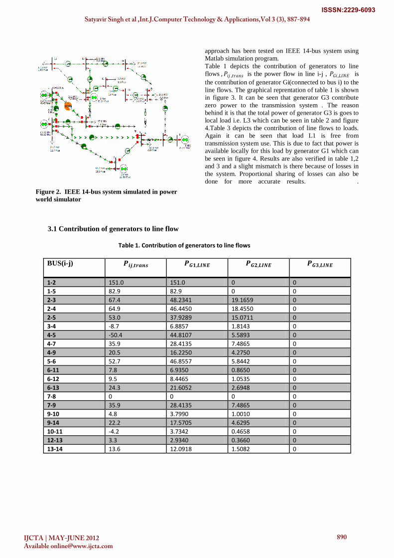
Figure 2. IEEE 14-bus system simulated in power

world simulator

approach has been tested on IEEE 14-bus system using

Matlab simulation program.

Table 1 depicts the contribution of generators to line

flows , 𝑃𝑖𝑗 ,𝑡𝑟𝑎𝑛𝑠 is the power flow in line i-j , 𝑃𝐺𝑖 ,𝐿𝐼𝑁𝐸 is

the contribution of generator Gi(connected to bus i) to the

line flows. The graphical reprentation of table 1 is shown

in figure 3. It can be seen that generator G3 contribute

zero power to the transmission system . The reason

behind it is that the total power of generator G3 is goes to

local load i.e. L3 which can be seen in table 2 and figure

4.Table 3 depicts the contribution of line flows to loads.

Again it can be seen that load L1 is free from

transmission system use. This is due to fact that power is

available locally for this load by generator G1 which can

be seen in figure 4. Results are also verified in table 1,2

and 3 and a slight mismatch is there because of losses in

the system. Proportional sharing of losses can also be

done for more accurate results. .

3.1 Contribution of generators to line flow

Table 1. Contribution of generators to line flows

BUS(i-j) 𝑷𝒊𝒋,𝒕𝒓𝒂𝒏𝒔

𝑷𝑮𝟏,𝑳𝑰𝑵𝑬

𝑷𝑮𝟐,𝑳𝑰𝑵𝑬

𝑷𝑮𝟑,𝑳𝑰𝑵𝑬

1-2 151.0 151.0 0 0

1-5 82.9 82.9 0 0

2-3 67.4 48.2341 19.1659 0

2-4 64.9 46.4450 18.4550 0

2-5 53.0 37.9289 15.0711 0

3-4 -8.7 6.8857 1.8143 0

4-5 -50.4 44.8107 5.5893 0

4-7 35.9 28.4135 7.4865 0

4-9 20.5 16.2250 4.2750 0

5-6 52.7 46.8557 5.8442 0

6-11 7.8 6.9350 0.8650 0

6-12 9.5 8.4465 1.0535 0

6-13 24.3 21.6052 2.6948 0

7-8 0 0 0 0

7-9 35.9 28.4135 7.4865 0

9-10 4.8 3.7990 1.0010 0

9-14 22.2 17.5705 4.6295 0

10-11 -4.2 3.7342 0.4658 0

12-13 3.3 2.9340 0.3660 0

13-14 13.6 12.0918 1.5082 0



890

ISSSN:2229-6093

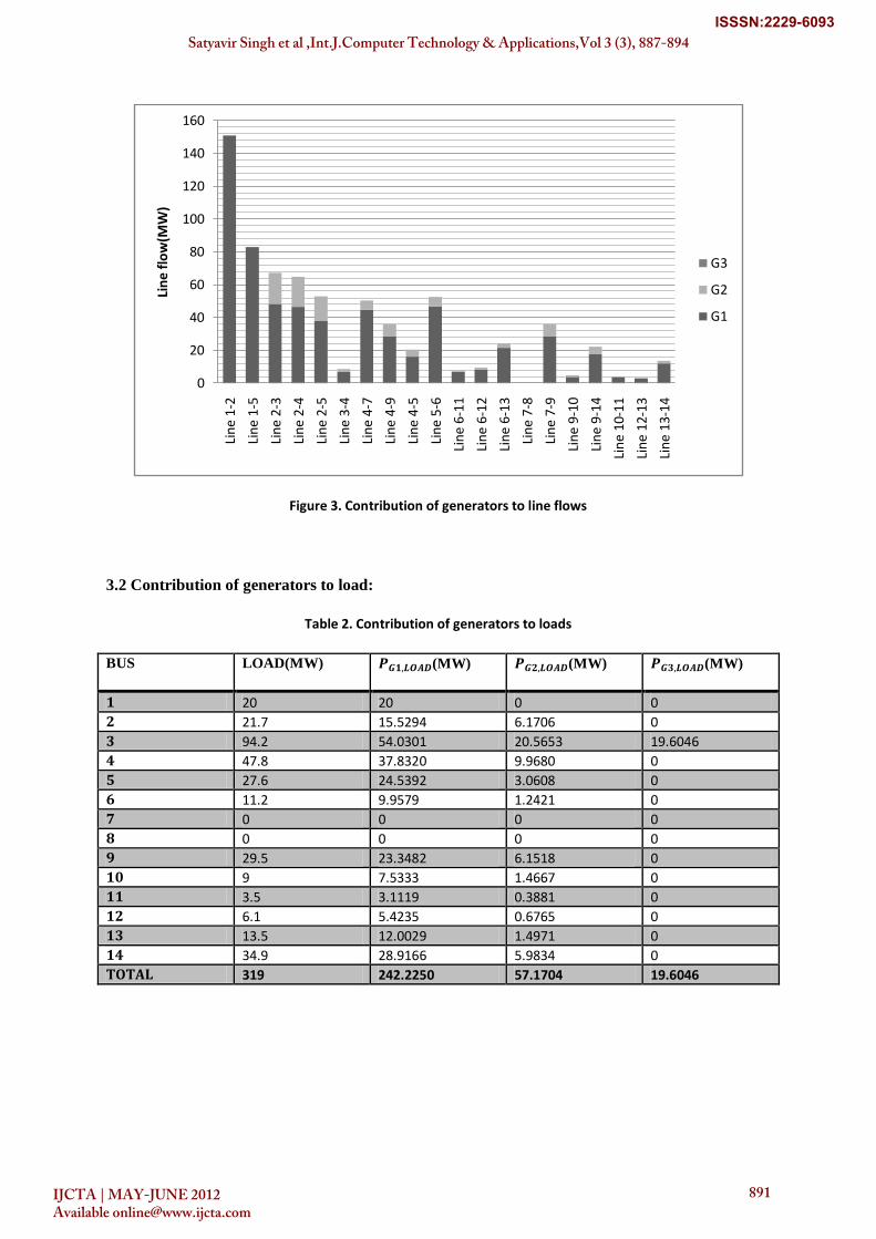
Figure 3. Contribution of generators to line flows

3.2 Contribution of generators to load:

Table 2. Contribution of generators to loads

BUS LOAD(MW) 𝑷𝑮𝟏,𝑳𝑶𝑨𝑫(MW)

𝑷𝑮𝟐,𝑳𝑶𝑨𝑫(MW)

𝑷𝑮𝟑,𝑳𝑶𝑨𝑫(MW)

1 20 20 0 0

2 21.7 15.5294 6.1706 0

3 94.2 54.0301 20.5653 19.6046

4 47.8 37.8320 9.9680 0

5 27.6 24.5392 3.0608 0

6 11.2 9.9579 1.2421 0

7 0 0 0 0

8 0 0 0 0

9 29.5 23.3482 6.1518 0

10 9 7.5333 1.4667 0

11 3.5 3.1119 0.3881 0

12 6.1 5.4235 0.6765 0

13 13.5 12.0029 1.4971 0

14 34.9 28.9166 5.9834 0

TOTAL 319 242.2250 57.1704 19.6046

0

20

40

60

80

100

120

140

160

Lin

e 1-

2

Lin

e 1-

5

Lin

e 2-

3

Lin

e 2-

4

Lin

e 2-

5

Lin

e 3-

4

Lin

e 4-

7

Lin

e 4-

9

Lin

e 4-

5

Lin

e 5-

6

Lin

e 6-

11

Lin

e 6-

12

Lin

e 6-

13

Lin

e 7-

8

Lin

e 7-

9

Lin

e 9-

10

Lin

e 9-

14

Lin

e 1

0-1

1

Lin

e 1

2-1

3

Lin

e 1

3-1

4

Lin

e fl

ow

(MW

)

G3

G2

G1



891

ISSSN:2229-6093

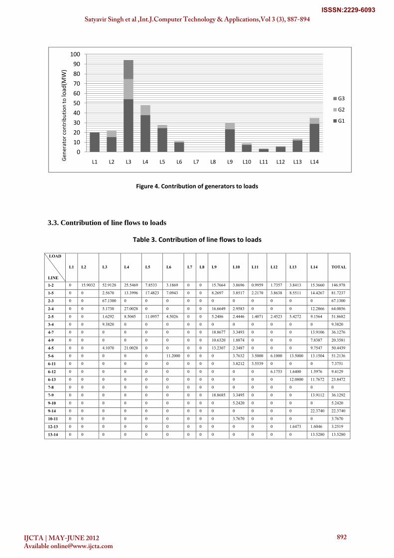
Figure 4. Contribution of generators to loads

3.3. Contribution of line flows to loads

Table 3. Contribution of line flows to loads

LOAD

LINE

L1 L2 L3 L4 L5 L6 L7 L8 L9 L10 L11 L12 L13 L14 TOTAL

1-2 0 15.9032 52.9128 25.5469 7.8533 3.1869 0 0 15.7664 3.8696 0.9959 1.7357 3.8413 15.3660 146.978

1-5 0 0 2.5670 13.3996 17.4823 7.0943 0 0 8.2697 3.8517 2.2170 3.8638 8.5511 14.4267 81.7237

2-3 0 0 67.1300 0 0 0 0 0 0 0 0 0 0 0 67.1300

2-4 0 0 5.1730 27.0028 0 0 0 0 16.6649 2.9583 0 0 0 12.2866 64.0856

2-5 0 0 1.6292 8.5045 11.0957 4.5026 0 0 5.2486 2.4446 1.4071 2.4523 5.4272 9.1564 51.8682

3-4 0 0 9.3820 0 0 0 0 0 0 0 0 0 0 0 9.3820

4-7 0 0 0 0 0 0 0 0 18.8677 3.3493 0 0 0 13.9106 36.1276

4-9 0 0 0 0 0 0 0 0 10.6320 1.8874 0 0 0 7.8387 20.3581

4-5 0 0 4.1070 21.0028 0 0 0 0 13.2307 2.3487 0 0 0 9.7547 50.4439

5-6 0 0 0 0 0 11.2000 0 0 0 3.7632 3.5000 6.1000 13.5000 13.1504 51.2136

6-11 0 0 0 0 0 0 0 0 0 3.8212 3.5539 0 0 0 7.3751

6-12 0 0 0 0 0 0 0 0 0 0 0 6.1753 1.6400 1.5976 9.4129

6-13 0 0 0 0 0 0 0 0 0 0 0 0 12.0800 11.7672 23.8472

7-8 0 0 0 0 0 0 0 0 0 0 0 0 0 0 0

7-9 0 0 0 0 0 0 0 0 18.8685 3.3495 0 0 0 13.9112 36.1292

9-10 0 0 0 0 0 0 0 0 0 5.2420 0 0 0 0 5.2420

9-14 0 0 0 0 0 0 0 0 0 0 0 0 0 22.3740 22.3740

10-11 0 0 0 0 0 0 0 0 0 3.7670 0 0 0 0 3.7670

12-13 0 0 0 0 0 0 0 0 0 0 0 0 1.6473 1.6046 3.2519

13-14 0 0 0 0 0 0 0 0 0 0 0 0 0 13.5280 13.5280

0

10

20

30

40

50

60

70

80

90

100

L1 L2 L3 L4 L5 L6 L7 L8 L9 L10 L11 L12 L13 L14Gen

erat

or

con

trib

uti

on

to

load

(MW

)

G3

G2

G1



892

ISSSN:2229-6093

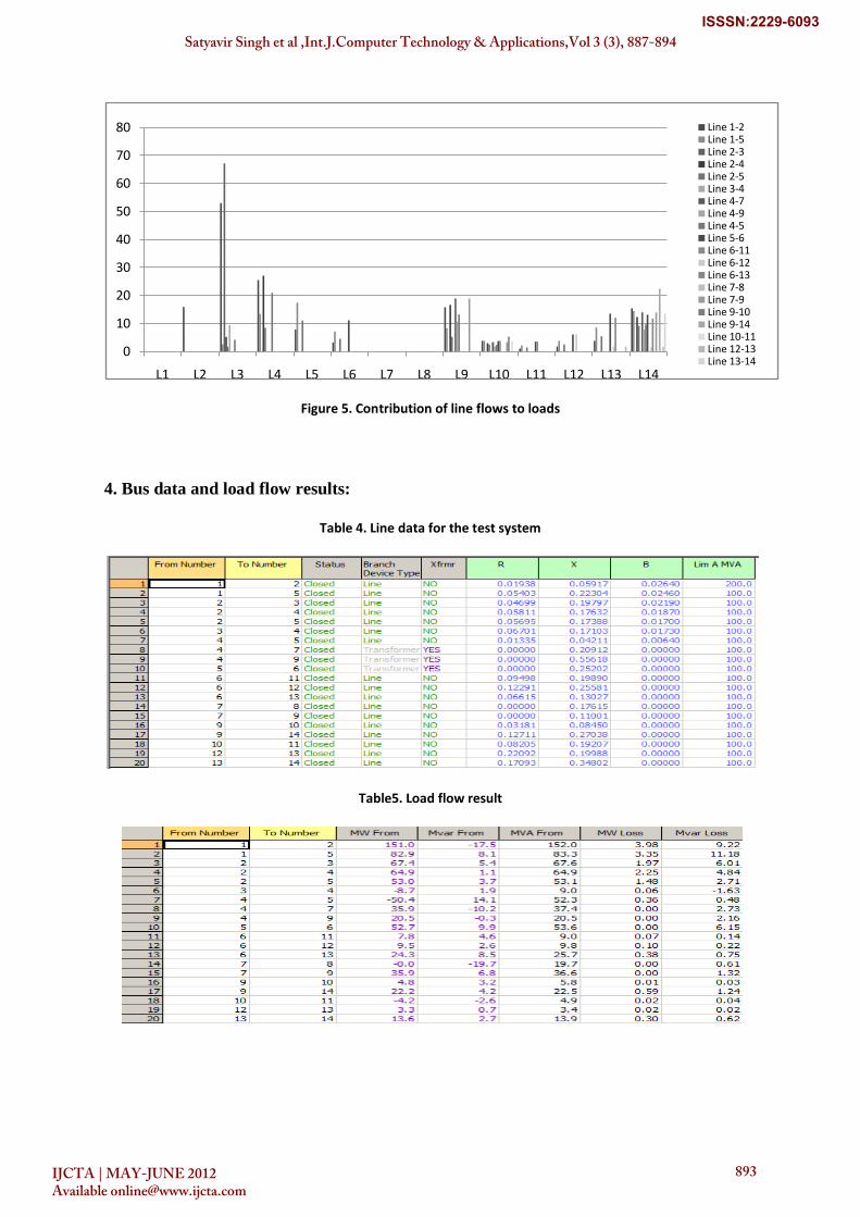
Figure 5. Contribution of line flows to loads

4. Bus data and load flow results:

Table 4. Line data for the test system

Table5. Load flow result

0

10

20

30

40

50

60

70

80

L1 L2 L3 L4 L5 L6 L7 L8 L9 L10 L11 L12 L13 L14

Line 1-2Line 1-5Line 2-3Line 2-4Line 2-5Line 3-4Line 4-7Line 4-9Line 4-5Line 5-6Line 6-11Line 6-12Line 6-13Line 7-8Line 7-9Line 9-10Line 9-14Line 10-11Line 12-13Line 13-14



893

ISSSN:2229-6093

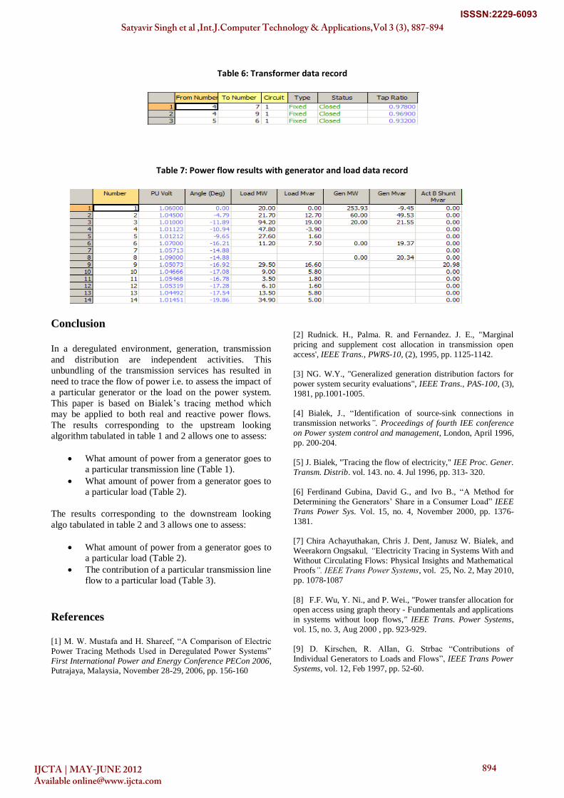
Table 6: Transformer data record

Table 7: Power flow results with generator and load data record

Conclusion

In a deregulated environment, generation, transmission

and distribution are independent activities. This

unbundling of the transmission services has resulted in

need to trace the flow of power i.e. to assess the impact of

a particular generator or the load on the power system.

This paper is based on Bialek’s tracing method which

may be applied to both real and reactive power flows.

The results corresponding to the upstream looking

algorithm tabulated in table 1 and 2 allows one to assess:

What amount of power from a generator goes to

a particular transmission line (Table 1).


a particular load (Table 2).

The results corresponding to the downstream looking

algo tabulated in table 2 and 3 allows one to assess:


a particular load (Table 2).

The contribution of a particular transmission line

flow to a particular load (Table 3).

References

[1] M. W. Mustafa and H. Shareef, “A Comparison of Electric

Power Tracing Methods Used in Deregulated Power Systems” First International Power and Energy Conference PECon 2006, Putrajaya, Malaysia, November 28-29, 2006, pp. 156-160

[2] Rudnick. H., Palma. R. and Fernandez. J. E., "Marginal

pricing and supplement cost allocation in transmission open

access', IEEE Trans., PWRS-10, (2), 1995, pp. 1125-1142.

[3] NG. W.Y., "Generalized generation distribution factors for

power system security evaluations", IEEE Trans., PAS-100, (3),

1981, pp.1001-1005.

[4] Bialek, J., “Identification of source-sink connections in

transmission networks”. Proceedings of fourth IEE conference

on Power system control and management, London, April 1996,

pp. 200-204.

[5] J. Bialek, "Tracing the flow of electricity," IEE Proc. Gener.

Transm. Distrib. vol. 143. no. 4. Jul 1996, pp. 313- 320.

[6] Ferdinand Gubina, David G., and Ivo B., “A Method for

Determining the Generators’ Share in a Consumer Load” IEEE

Trans Power Sys. Vol. 15, no. 4, November 2000, pp. 1376-

1381.

[7] Chira Achayuthakan, Chris J. Dent, Janusz W. Bialek, and

Weerakorn Ongsakul, “Electricity Tracing in Systems With and

Without Circulating Flows: Physical Insights and Mathematical Proofs”. IEEE Trans Power Systems, vol. 25, No. 2, May 2010,

pp. 1078-1087

[8] F.F. Wu, Y. Ni., and P. Wei., "Power transfer allocation for open access using graph theory - Fundamentals and applications

in systems without loop flows," IEEE Trans. Power Systems,

vol. 15, no. 3, Aug 2000 , pp. 923-929.

[9] D. Kirschen, R. AlIan, G. Strbac “Contributions of

Individual Generators to Loads and Flows”, IEEE Trans Power

Systems, vol. 12, Feb 1997, pp. 52-60.



894

ISSSN:2229-6093

Power Tracing in a Deregulated Power System : IEEE 14-Bus … · Power Tracing in a Deregulated...

Documents

Transcript of Power Tracing in a Deregulated Power System : IEEE 14-Bus … · Power Tracing in a Deregulated...