Power system stability analysis of cable based HVAC transmission grids

with reactive power compensation

Master thesis by

Foo Yi Wern&

Laurids Martedal Bergholdt Dall

June 2016

Title: Power system stability analysis of cable based HVAC

transmission grids with reactive power compensation

Semester / theme: 10th semester / Master thesis

Project period: 1.2.2016 to 1.6.2016

ECTS: 30

Supervisor: Filipe Miguel Faria da Silva

Project group: EPSH4-1031

Yi Wern Foo

Laurids Martedal Bergholdt Dall

SYNOPSIS:This thesis presents a study of the elec-

tromechanical dynamics associated with the

implementation of long HVAC cables in

power transmission. Transient stability and

large-disturbance voltage stability of generic

multi-machine power systems is assessed by

RMS simulations in DIgSILENT PowerFac-

tory. The stability performance of the OHL

base case system is compared against an

equivalent cable system. Results show that

the 100 % compensated equivalent cable sys-

tem has longer CCT than the OHL base sys-

tem in most cases. Increasing the SR com-

pensation degree may improve the CCT, while

voltage stability analysis show that under-

compensation improve the V, P load-ability.

The cable system displays larger Pmax than

the OHL base system. An advantage of the

cable system is the availability of switch-able

SRs. By decreasing XSR during a large dis-

turbance, the capacitive current generated by

the cables is injected into the network to im-

pose a voltage. Case studies show that SR-

switching can improve system voltages. A

smooth voltage recovery is achieved by se-

quentially switching the buses measuring the

lowest voltages. Further work is required in

order to generalize and quantify the proper-

ties of SR-switching.

Copies: 4

Pages, total: 189

Appendix: 10

Supplements: 1 CD

By signing this document, each member of the group conrms that all group

members have participated in the project work, and thereby all members are

collectively liable for the contents of the report. Furthermore, all group mem-

bers conrm that the report does not include plagiarism.

Preface

This thesis is written by group EPSH4-1031, during the 4th and nal semester of

the 'Electrical Power Systems and High Voltage Engineering' programme at Aalborg

University. The work presented has been carried out from the 1st of February to the

1st of June 2016.

We would like to direct a special thank you to our supervisor, Filipe Faria da Silva for

guidance, comments and weekly meetings throughout the project period.

Reading Guide

This thesis is divided in eight chapters and ten appendices, containing references,

illustrations, tables and equations. The literature references are referred to according

to the IEEE citation style, numbered in the order of appearance. The bibliography is

located at the end of the report, containing further information about the source. Books

are listed with author, year, title, edition and publisher; Websites are listed with author,

title, date and URL. Figures, tables and equation will be referred to by a chapter and a

number [chapter, number], including a word or an abbreviation indicating what is being

referred to. The words/abbreviation are Figure for illustrations and Table for tables. If

no reference is given on a gure it means that the gure was created by the project group.

Software

The following software has been used during the project:

DIgSILENT PowerFactory version 15.1.6

LaTeX is used to write the report.

Matlab is used for coding scripts and plotting.

v

Abstract

Danish TSO Energinet.dk is in the process of undergrounding parts of the AC transmission

grid in Denmark. Undergrounding involves the replacement of conventional overhead line

(OHL) transmission with underground cables. The electrical behaviour of a HVAC cable

is substantially dierent to that of an equivalent OHL. The most signicant dierence is

the capacitance, where cables display values typically 10-20 times greater than OHL.

The focus of this thesis is to study the electromechanical dynamics associated with the

implementation of long HVAC cables in the power transmission network. The main

objective is to assess and study the transient stability and large-disturbance voltage

stability of generic multi-machine power systems.

This is accomplished by simulating large-disturbance electromechanical transients in

DIgSILENT PowerFactory. The analysis is initiated on a simple single-machine innite

bus system, and is expanded to the IEEE 9-bus and 39-bus multi-machine power systems.

The stability performance of the OHL base case system is compared against an equivalent

cable system.

Transient stability studies are performed with variations to fault locations, and critical

clearing time (CCT) is chosen as stability index. For voltage stability assessment both

steady state analysis of V, P and Q,V -characteristics and RMS simulation based voltage

trajectory analysis are performed.

Comparison of the transient stability performance in both SMIB and multi-machine

systems show that the equivalent cable system with 100 % compensation has consistently

longer CCT than the OHL base system, provided that the corresponding shunt reactors

(SR) of the faulted line are disconnected when the line is taken out of service.

Increasing the SR compensation degree has an improving eect on the CCT. This was

tested up to 115 %, and is a conrmation of the ndings in the state of the art.

However, this result is not explicitly conclusive for every aspect of power system stability.

In contradiction the voltage stability analysis show that under-compensation of cables

improve the V, P load-ability of the network. Being under-compensated, the cables supply

reactive power to line inductance, inductive loads and transformers locally. Hence the

optimal compensation degree is concluded to be a balance of both synchronous generator

excitation level and the ability to supply reactive power locally in the network.

The V, P -characteristics in both 9-bus system and 39-bus system show that the 100 %

compensated equivalent cable system display higher steady state load-ability than the

OHL base system. This result is in line with the overall CCT observations, and is ascribed

to the L and R dierence. Similarly Q,V -curves of the equivalent cable systems prove to

be slightly steeper, indicating lower voltage sensitivity to changes in reactive power ow.

The bus voltages following large-disturbances are evaluated against an under-voltage limit.

vii

An advantage of the cable based system is the presence of SRs. The cable based system is

equipped with a signicant amount of local reactive power support, by assuming that SRs

can switched in and out of service as fast as necessary. By decreasing the shunt reactance

during an electromechanical transient, the large amount of capacitive current generated

by the cables is injected into the network inductance and thereby imposing a voltage.

It is shown for various cases that SR-switching can improve voltage trajectories to satisfy

the under-voltage limit. This ability is unavailable in the OHL base system, where

compensation for steady-state operation is unnecessary.

It is concluded that the SR-switching should be performed progressively to reduce the

risk of transient over-voltages. A smooth voltage recovery can be achieved by sequentially

switching the buses measuring the lowest voltages. The overall system improvement should

be considered and not limited to the lowest voltage buses. The amount of SR-switching

necessary could be based on the magnitude of the post-disturbed voltage and dQ/dV -

sensitivities of the network. Further work is required in order to generalize and quantify

the properties of SR-switching.

Furthermore, it is shown how SR-switching may reduce the need of dynamic voltage

regulation in the form of FACTS. By performing SR-switching the necessary capacity of

STATCOMs may be signicantly reduced or completely substituted.

viii

Table of contents

Chapter 1 Introduction 1

1.1 Background . . . . . . . . . . . . . . . . . . . . . . . . . . . . . . . . . . . . 1

1.2 Types of power system stability . . . . . . . . . . . . . . . . . . . . . . . . . 6

1.3 Principles of transient stability . . . . . . . . . . . . . . . . . . . . . . . . . 8

1.4 Principles of voltage stability . . . . . . . . . . . . . . . . . . . . . . . . . . 14

1.5 Transmission lines in power system stability studies . . . . . . . . . . . . . . 20

1.6 State of the art review . . . . . . . . . . . . . . . . . . . . . . . . . . . . . . 25

Chapter 2 Problem statement and methodology 35

2.1 Problem statement . . . . . . . . . . . . . . . . . . . . . . . . . . . . . . . . 35

2.2 Delimitations . . . . . . . . . . . . . . . . . . . . . . . . . . . . . . . . . . . 36

2.3 Methodology . . . . . . . . . . . . . . . . . . . . . . . . . . . . . . . . . . . 37

Chapter 3 Stability analysis of single-machine innite bus system 39

3.1 Single-machine innite bus system . . . . . . . . . . . . . . . . . . . . . . . 39

3.2 Introducing the DIgSILENT PowerFactory SMIB system . . . . . . . . . . . 41

3.3 Sensitivity study of line parameters on the SMIB system . . . . . . . . . . . 44

3.4 Comparison of OHL and cable transmission lines in the SMIB system . . . 54

Chapter 4 Transient stability analysis 59

4.1 Introduction . . . . . . . . . . . . . . . . . . . . . . . . . . . . . . . . . . . . 59

4.2 IEEE 9-bus transient stability analysis . . . . . . . . . . . . . . . . . . . . . 61

4.3 IEEE 39-bus transient stability analysis . . . . . . . . . . . . . . . . . . . . 68

4.4 Transient stability summary . . . . . . . . . . . . . . . . . . . . . . . . . . . 74

Chapter 5 Large-disturbance voltage stability analysis: IEEE 9-bus

system 77

5.1 Load modelling in voltage stability analysis . . . . . . . . . . . . . . . . . . 77

5.2 Q,V-characteristics of load buses in the IEEE 9-bus system . . . . . . . . . 79

5.3 Voltage stability of Bus 8 in the IEEE 9-bus system . . . . . . . . . . . . . 81

5.4 Discussion of reactive power capability limits in the IEEE 9-bus system . . 83

5.5 Voltage trajectory analysis of Bus 8 in the IEEE 9-bus system . . . . . . . . 86

5.6 Forcing voltage instability in the IEEE 9-bus system . . . . . . . . . . . . . 90

5.7 Summary of voltage stability analysis in the IEEE 9-bus system . . . . . . . 100

Chapter 6 Large-disturbance voltage stability analysis: IEEE 39-bus

system 103

6.1 Identication and characterization of weak areas in the IEEE 39-bus system 104

6.2 V,P-characteristics of areas in the IEEE 39-bus system . . . . . . . . . . . . 107

6.3 Q,V-characteristics of areas in the IEEE 39-bus system . . . . . . . . . . . . 109

6.4 Large-disturbance case studies in the IEEE 39-bus system . . . . . . . . . . 111

6.5 Summary of voltage stability analysis in the IEEE 39-bus system . . . . . . 126

ix

Chapter 7 Discussion of results 129

7.1 Comparison of results with published research . . . . . . . . . . . . . . . . . 129

7.2 Discussion of methodology and validity of results . . . . . . . . . . . . . . . 131

7.3 Future work . . . . . . . . . . . . . . . . . . . . . . . . . . . . . . . . . . . . 133

Chapter 8 Conclusion 135

Bibliography 137

Appendix A Accounting for capacitance in SMIB systems 141

Appendix B Basic voltage regulation and reactive power control of

synchronous generators 147

B.1 Control of active and reactive power . . . . . . . . . . . . . . . . . . . . . . 147

B.2 Automatic voltage regulator . . . . . . . . . . . . . . . . . . . . . . . . . . . 151

B.3 Excitation system inuence on power system stability . . . . . . . . . . . . 152

B.4 Inuence of governors and power system stabilizers compared to AVR . . . 154

Appendix C Modelling parameters in 9-bus and 39-bus systems 157

C.1 9-bus system . . . . . . . . . . . . . . . . . . . . . . . . . . . . . . . . . . . 157

C.2 39-bus system . . . . . . . . . . . . . . . . . . . . . . . . . . . . . . . . . . . 159

Appendix D DIgSILENT Programming Language used in studies 163

Appendix E Pole-slip function in PowerFactory 167

Appendix F PowerFactory simulation results for 9-bus and 39-bus system171

Appendix G Simple model of a generic STATCOM in DIgSILENT

PowerFactory 179

G.1 Modications to the generic model . . . . . . . . . . . . . . . . . . . . . . . 180

Appendix H Additional case studies of SR-switching and STATCOM 183

Appendix I Utilizing Q,V-characteristics for SR-switching 185

Appendix J CD content 189

x

List of symbols

Table 1. List of symbols used in this report - Part 1.

Symbol Unit Name

C [F] Capacitance

d [m] Distance

e [-] Exponent coecient

E [V] Voltage

F [-] Factor

G [S] Conductance

H [MWs/MVA] Inertia constant

I [A] Current

J [kg ·m2] Mechanical inertia

K [-] Gain

k [-] Coecient

l [m] Length

L [H] Inductance

n [-] Number of

P [W] Active Power

Q [var] Reactive power

p, q [-] Coecients

R [Ω] Resistance

S [VA] Apparent power

T [N ·m] Torque

T [s] Time constant

t [s] Time

V [V] voltage

X [Ω] Reactance

x [-] State variable

Z [Ω] Impedance

z [m] Distance

When a symbol has a subscript, the text is used to refer to a specic value,

function or component, for example xl may refer to the line reactance.

xi

Table 2. List of symbols used in this report - Part 2.

Symbol Unit Name

β [rad/m] Phase constant

δ [deg] Power angle

Γ [-] Coecient

λ [m] Wavelength

ω [rad/s] Rotational speed

ω [rad/s] Electrical Frequency

θ [deg] Power factor angle

When a symbol has a subscript, the text is used to refer to a

specic value, function or component, for example ωs may refer to

the synchronous speed.

Table 3. List of abbreviations used in this report.

Abbreviation Name

AC Alternating Current

AVR Automatic Voltage Regulator

CCT Critical Clearing Time

DFIG Doubly Fed Induction Generator

DPL DIgSILENT Programming Language

FACTS Flexible AC Transmission Systems

HVAC High Voltage Alternating Current

HVDC High Voltage Direct Current

OEL Over-Excitation Limiter

OHL Overhead Line

OLTC On Load Tap Changer

PF Power Factor

PSS Power System Stabilizer

PV Photovoltaic

SG Synchronous Generator

SI Surge Impedance

SIL Surge Impedance Load

SMIB Single-Machine Innite Bus

SR Shunt Reactor

STATCOM Static Compensator

SVC Staticc Var Compensator

TL Transmission Line

TSO Transmission System Operator

VSC Voltage Source Converter

xii

Introduction 1The focus of this thesis is to investigate the electromechanical dynamics associated with the

implementation of long HVAC cables in the power transmission network. More specically

multi-machine power systems with various line parameters are to be analysed with respect

to transient and voltage stability. A special emphasis is directed towards the issue of

reactive power compensation, and its signicance in a cable based power system.

The following chapter introduces the basic concepts concerning power system stability,

while describing the background of the project. The terms transient stability and

voltage stability are discussed and dened according to relevant IEEE and CIGRE

recommendations to specify the terminology according to the project goals. The main

dierences on overhead line (OHL) and cable based networks are briey discussed, with

focus on the important characteristics in stability studies. Finally, the most recent research

in stability studies with HVAC cable power systems is discussed and the initiating problem

is described.

1.1 Background

Power system stability is a mature and well researched branch of power system analysis.

Mathematical models and tools for stability analysis have been developed since the early

1920s, where the rst instability issues in AC power systems were experienced [1]. Accurate

stability studies demand thorough dynamic modelling of power system components,

with particular emphasis on the dierential equations describing the electromechanical

dynamics of the electrical machinery. The dynamic models for the most traditional power

system components and their application are well described by the author of [2], and is

widely recognized as the state of the art for power system stability studies.

Power system stability is an extensive technical term, involving every aspect of power

generation, transmission and distribution. Thus, assessing the stability of a given power

system can turn out to be a cumbersome and complex task. In year 2004 the authors of

[3] published the eorts of a combined IEEE and CIGRE taskforce with the objectives

of dening and classifying various power system stability topics and categorizing power

system instability phenomena. Furthermore the authors of [3] highlight the realisation

that complete mathematical modelling of power system stability is generally unachieved,

especially for large systems. Typically what is referred to as partial stability analysis is

applied in studies of transient and voltage stability [3]. Here the focus is on the behaviour

of a subset of variables, while the remaining system states may be ignored for simplicity.

Thus, when analysing power system stability, simplications are generally favourable. As

a result, careful attention should be paid towards the absence of unmodelled interactions

of the power system environment.

1

Examples could be unmodelled electrical machinery dynamics and controls, protection

topologies and variations of line switching, altering the system topology.

Instability of the power system can in the most severe cases result in a total system

collapse leading to what is often referred to as a blackout. Fortunately blackouts are

rare, but historically they do occur, even as stability-improvement methods have been

continuously developed and implemented. On the 14th of August 2003 the United States

and Canada experienced a blackout in the north-eastern part of North America. A task

force was formed in order to investigate the causes of the blackout and to elaborate future

preventive methods. However, the answer to the cause of the system collapse turned out

not to be a simple one, as stated by the task force in [4]. Largely the initial cause is

described as a failure of both equipment and human action in control center of a local

energy company, when three 345-kV and one 138-kV transmission lines started tripping

due to transient currents related to line faults caused by partial discharges to the nearby

vegetation. The following undetected overloading of several transmission lines, combined

with an already voltage depressed power system due to inadequate reactive power supply,

caused an cascading outage throughout the region. The aftermath of the 2003 blackout

was a wake-up call resulting in government enforced regulations and an extensive use of

the terminologies: power system reliability and security.

For scientists and engineers working in the eld of power system stability, the terms

reliability and security may seem redundant in the presence of the technical stability

denitions. However, the authors of [3] describe power system reliability as "the ability

to supply adequate electric service on a nearly continuous basis, with few interruptions

over an extended time period" and power system security as "the degree of risk the power

systems ability to survive imminent disturbances (contingencies) without interruption of

customer service". Evidently these formulations are easily confused with the classical

denition of power system stability: "The continuance of intact operation following a

disturbance", but the members of the joint IEEE and CIGRE task force seek to distinguish

between the terminologies. Power system contingencies involving explosive cable failures,

fall of transmission towers or sabotage, are recognized as reliability issues, while security

issues are dened as the resulting consequences of power system instability. However,

the system wide behaviour following a disturbance, regardless of the cause or terminology

used, is dependant of the electromechanical behaviour of the power system and the classical

electrical engineering denitions. Thus, the subject of power system stability is treated

in the classical term throughout this thesis, and the terms reliability and security are not

applied.

Although stability is a mature topic in power systems, on both theoretical and practically

applied level, it is a topic which demands continuous attention. The power system is

changing, and now possibly faster than ever. On a global level the amount of renewable

power capacity is increasing, and throughout year 2014 renewables made up 58.5 %

of the globally installed capacity that year. Thus, reaching a total capacity gure of

1.712 GW by the end of year 2014, corresponding to 22.8 % of the global electricity demand

[5]. Renewable resources such as wind and solar imply a uctuating and uncontrollable

nature of power supply, consequently demanding extra focus on the constant balancing of

generation and load, and increasing the complexity of power system control.

2

Furthermore, the implementation of renewables has inuenced the transient stability limits

of the power system. According to the authors of [6], the inuence of a high penetration

of doubly-fed induction generators (DFIG) can have an either benecial or destructive

impact on power system stability. The impact of wind power penetration is largely

dependant on the DFIG insertion point in the grid and the location of disturbances. An

increasing problem is the loss of mechanical inertia utilized in maintaining synchronism,

and delivering short-circuit power during large disturbances. On the other hand, the

increased penetration of DFIG can result in an indirect dampening eect of the power

system oscillations associated with instabilities, due to the reduction in synchronous

generators (SG) participating. However, with the wind penetration numbers reaching

as high as 42.1 % [7], the impact of wind power on stability limits is arguably mainly

negative. Similarly, the impacts of high photovoltaic (PV) penetration is investigated in

[8]. The results indicate that power systems with high PV penetration levels (20 % to 50

%), suer from large bus voltage dips during transients, indicating the need for dynamic

reactive power compensation in order to mitigate possible voltage collapses.

In order to distribute the large amount of uctuating power produced from renewables,

some countries are expanding their transmission systems by investing in interconnections

across country borders. One of the benets of such interconnections is the ability to

utilize regional unbalances in generation and load, and by cross country transmission and

distribution, limit local bottlenecks. Danish TSO Energinet.dk is participating in the

preparations of two new high-voltage direct current (HVDC) connections in the North

Sea. The COBRAcable (700 MW), which is expected to connect Denmark and Holland

by 2019 [9] and the Viking Link (1.4 GW), connecting Denmark and England by 2022

[10]. Furthermore, Energinet.dk is cooperating with TenneT in Germany on expanding

the existing 1.5 GW HVAC connection crossing the Denmark-Germany border to 2.5 GW

by 2020 [11]. Finally, near the construction of the 600 MW Kriegers Flak oshore wind

farm, is the establishment of a 400 MW HVDC connection between East Denmark and

Germany by 2018 [12].

The increasing interconnection of power systems, on both national and international level,

is inuencing the stability limits of the system signicantly. Expansion of the power

system, by the addition of transmission lines, improves the power system's ability to

remain stable following contingencies, such as the loss of generation or transmission lines.

As power can be transmitted between generation and load without violation of stability

limits. The authors of [13] investigate how issues with uncontrollable cascading eects

of large interconnected power systems can be mitigated by the implementation of HVDC

connections with voltage-source converters, such as the ones being installed in Denmark.

It is found that HVDC connections acts as blocking of power angle oscillations related to

transient stability, and provides voltage stability improvement by reactive power control.

Thus, interconnecting by HVDC-VSC is expected to have an improving eect on power

system stability.

3

Another major topological change of the danish power system, is the ongoing

undergrounding of the high voltage AC grid, as published by Energinet.dk in [14] and

[15]. In the grid development plan it is stated that it has been politically decided, to

replace a big part of the overhead lines in the transmission network with underground

transmission cables. The main motivation is to improve the aesthetic look of the danish

landscape. Traditionally the majority of power system transmission lines are OHL, and

a CIGRE study [16] show that underground cables are mainly represented in 50 kV to

109 kV distribution networks. Figure 1.1 shows a map of the future Danish high voltage

power system. The 132 kV to 150 kV overhead lines (OHL) are to be fully replaced by

HVAC cables, while the 400 kV lines are to be partially replaced by cables.

Figure 1.1. Future Danish power system anno 2032 according to Energinet.dk grid development

plans, showing the 150 kV to 400 kV system [14]. The plan does not display the

Viking Link.

4

The electrical behaviour of a HVAC cable is substantially dierent to that of an equivalent

OHL. The most signicant dierence is the capacitance, where cables display values

typically 10-20 times greater than OHL [17]. As a result the HVAC cables generally

inject a substantial amount of capacitive current, whereas OHLs mainly draw inductive

current. Consequently, the change from OHL to cable-based power transmission imply

a drastic change of reactive power ow of the system. Historically, transmission line

susceptance has been ignored for short line modelling (lengths shorter than 80 km), due

to negligible capacitance [2]. However, for cable modelling such practice is erroneous for

any given length. As voltage levels are increased (400 kV and higher) for both OHL and

cables, the reactive power generated by even small values of capacitance and line lengths

is considerable. This is due to the V 2 proportionality. In order to avoid over-voltages

during steady state operation HVAC cables must be compensated by the connection of

inductive shunt reactors, whereas OHLs are compensated by series capacitors if necessary.

However, the implementation of HVAC tranmission cables does not only aect the steady

state performance of the system. The nature of electromagnetic transients in power

transmission cables is analysed and discussed by the authors of [18], explaining how the

physical characteristics of cables alter line parameters and eectively inuence switching

phenomena, travelling waves and more.

Being established, that the topologically fundamental change from OHL to cables in the

HVAC power system, has a signicant inuence on multiple aspects of the power system as

a whole, it becomes relevant to consider the impact on power system stability. As described

in [2] transmission network topology inuence both transient stability and voltage stability.

The transient stability limits are altered as equivalent network impedances inuence the

non-linear power-angle relationship of the interacting electrical machinery. An inuence

which is present in both pre-disturbance, disturbance and post-disturbance conditions.

The large-disturbance voltage stability is mainly an issue addressing the balance of reactive

power at local system weak-points during and following major disturbances, such as line

faults and switching. Thus, it is impending to believe that there exist one or more voltage

stability related consequences, following the change from OHL to cable based transmission.

Undergoing any major system restructuring, such as the one described by Energinet.dk

in [14], it seems vital to consider a revaluation of the power system stability. However, a

problem appear to be the lack of available research and guidelines on the topic of HVAC

cables in power system stability studies. Some publications address the issue, such as

[19] [20] [21] [22]. These studies are discussed in further detail in Section 1.6.1. A quick

review reveal that the few studies published are very dierent in their use of stability

terminology and methodology towards the topic of HVAC cables in stability analysis.

The study presented in [19] is limited to a simple single-machine innite bus (SMIB) with

focus on transient stability. The research in [20] treat small-signal voltage stability in the

case of a specic island grid in Taiwan. While [21] address power system stability in the

context of undergrounding of a part of the Dutch HV network, more similar to the Danish

case. And nally [22] investigates the idea of utilizing a mixed OHL and cable system for

mutual reactive power compensation.

5

Due to the sparsity in available literature, and motivated by the Danish grid development

plans, this thesis seek to investigate both transient and voltage stability limits for

multimachine power systems with cable based HVAC transmission. In the case that

instability issues are discovered, the aim is to discus and point towards possible solutions.

The focus in this thesis, is the use of power system simulation software and generic power

system models, to explore the stability during large disturbances. While the results are

to be discussed on the basis of the theoretical principles, a detailed mathematical study

of the stability phenomena is not the objective. Instead, parametric sensitivity studies

are performed in order to provide understanding and highlight the key issues of assessing

stability of power transmission networks with HVAC cables.

In summary the question to be answered is: How does undergrounding of the HVAC power

system aect power system stability limits, and how should reactive power compensation

be utilized to improve the stability?

1.2 Types of power system stability

Power system stability is a major issue of concern for continuous system operations.

However it comes in many forms and cannot be treated as a single whole entity. Therefore

it is important to identify and dene the various instabilities and their respective dynamic

behaviour in a system for assessment purposes.

The type of dynamic behaviour can be classied according to its response time.

Electromagnetic transients are the fastest transients which occur in the time range of

µs and are related to events such as switching surges and lightning propagation [23]. In

contrast, electromechanical transients are slower transients which can be detected in the

time span of 3-10 s and up to a few minutes. The project focuses only on the issues

regarding electromechanical dynamics namely transient stability and voltage stability.

The theory and principle behind each of these stabilities are further expanded in Sections

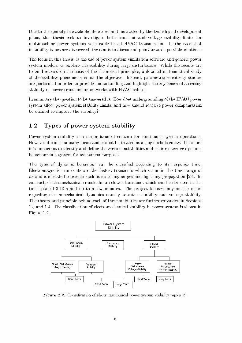
1.3 and 1.4. The classication of electromechanical stability in power system is shown in

Figure 1.2.

Figure 1.2. Classication of electromechanical power system stability topics [3].

6

1.2.1 Transient stability and voltage stability

As can be seen from Figure 1.2, transient stability is a subform of rotor angle stability. In

synchronous generators terminology, rotor angle could also be referred to as power angle

and load angle whereby the terms are inter-changable. For standardization purposes, the

term power angle will be used from here onwards in the project. According to CIGRE

and IEEE, transient stability is dened as the "ability of the power system to maintain

synchronism when subjected to a severe disturbance [3]." Examples of large disturbances

are fault on transmission line and loss of generating units.

Transient instability of a synchronous generator involves a deviation of its power angle

beyond the critical value which causes loss of synchronism. The duration of transient

could vary from three to ve seconds up to 10 seconds depending on dierent factors

[2]. It is practised by authors in [24] to carry out simulations up to 10 seconds after the

disturbance in order to verify unstable cases.

Figure 1.3 depicts the time response of the power angle following a disturbance. Case

1 represents the instantaneous form of instability and is commonly called rst-swing

instability where the power angle is increased continously beyond its critical value. As for

large power systems, instability may not be from the rst swing but as a consequence of

cascading interarea oscillations between groups of machines as shown in Case 2 [2].

Power Angle, δ [deg]

Time [s]0.5 1.0 1.5 2.0 2.5 3.0 3.50

Case 2

Case 1

Figure 1.3. Power angle response to a disturbance.

Voltage stabiity is the "ability to maintain steady voltages at all buses in the system after

being subjected to a disturbance [3]." It is also categorised according to the severity of

the disturbance to the power system. Small signal voltage stability is analysed when the

system experiences small perturbations. In this thesis, voltage stability refers to the large

disturbance voltage stability during which the power system is subjected to disturbances

of similar severity as transient stability.

It is common that angle stability and voltage stability do not present the eects

individually. Instead, often instability in one would greatly aect the other due to

strong coupling between them following large disturbances [3]. Though it may be hard

to distinguish between the two, it is important to identify the underlying causes of the

problem for precise protective operations. The basis of distinction lies in the variable

which is more evident in the instability [3].

7

1.3 Principles of transient stability

This section illustrates the dynamic response of a synchronous machine in a system when

subjected to a disturbance and provides an elementary view on transient stability. The

topic related to multi-machine systems will also be briey discussed.

1.3.1 Single machine innite bus system

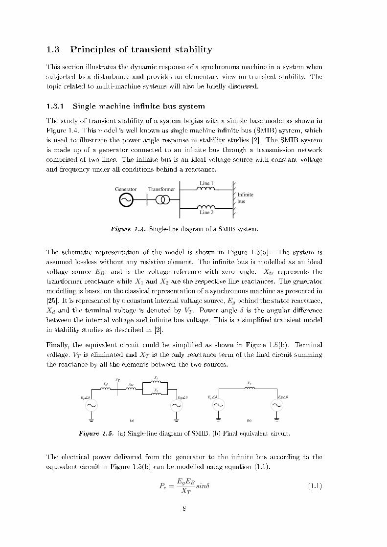
The study of transient stability of a system begins with a simple base model as shown in

Figure 1.4. This model is well known as single machine innite bus (SMIB) system, which

is used to illustrate the power angle response in stability studies [2]. The SMIB system

is made up of a generator connected to an innite bus through a transmission network

comprised of two lines. The innite bus is an ideal voltage source with constant voltage

and frequency under all conditions behind a reactance.

GeneratorInfinite bus

TransformerLine 1

Line 2

Figure 1.4. Single-line diagram of a SMIB system.

The schematic representation of the model is shown in Figure 1.5(a). The system is

assumed lossless without any resistive element. The innite bus is modelled as an ideal

voltage source EB, and is the voltage reference with zero angle. Xtr represents the

transformer reactance while X1 and X2 are the respective line reactances. The generator

modelling is based on the classical representation of a synchronous machine as presented in

[25]. It is represented by a constant internal voltage source, Eg behind the stator reactance,

Xd and the terminal voltage is denoted by VT . Power angle δ is the angular dierence

between the internal voltage and innite bus voltage. This is a simplied transient model

in stability studies as described in [2].

Finally, the equivalent circuit could be simplied as shown in Figure 1.5(b). Terminal

voltage, VT is eliminated and XT is the only reactance term of the nal circuit summing

the reactance by all the elements between the two sources.

Eg EB 0δ

VTXd Xtr

X1

X2

EB 0Eg δ

XT

(a) (b)

Figure 1.5. (a) Single-line diagram of SMIB. (b) Final equivalent circuit.

The electrical power delivered from the generator to the innite bus according to the

equivalent circuit in Figure 1.5(b) can be modelled using equation (1.1).

Pe =EgEBXT

sinδ (1.1)

8

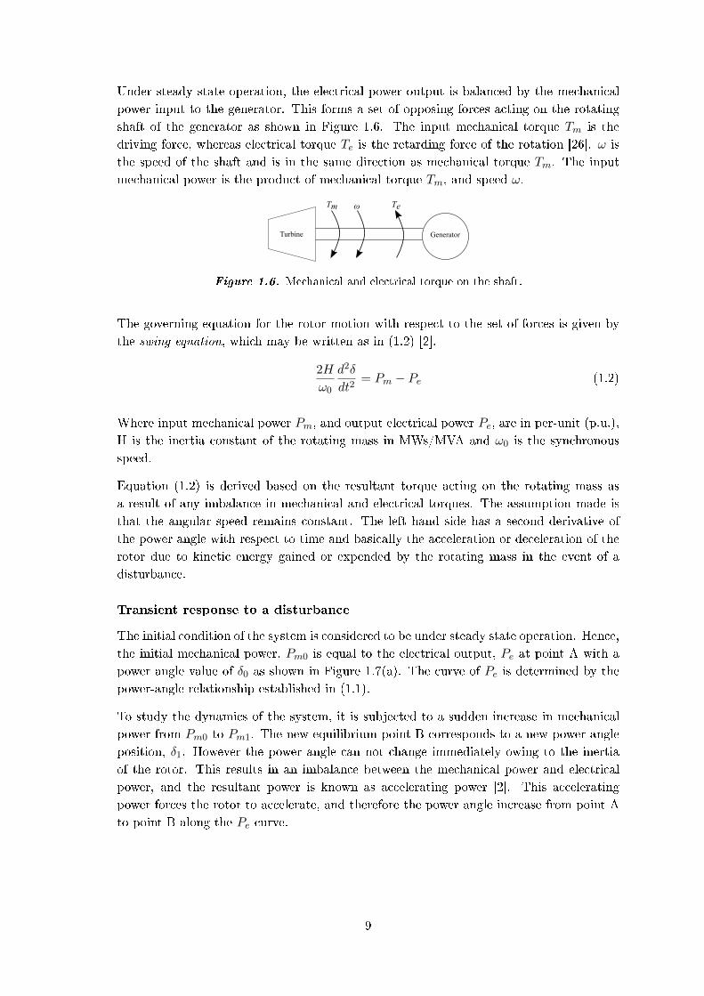
Under steady state operation, the electrical power output is balanced by the mechanical

power input to the generator. This forms a set of opposing forces acting on the rotating

shaft of the generator as shown in Figure 1.6. The input mechanical torque Tm is the

driving force, whereas electrical torque Te is the retarding force of the rotation [26]. ω is

the speed of the shaft and is in the same direction as mechanical torque Tm. The input

mechanical power is the product of mechanical torque Tm, and speed ω.

Turbine Generator

Tm Teω

Figure 1.6. Mechanical and electrical torque on the shaft.

The governing equation for the rotor motion with respect to the set of forces is given by

the swing equation, which may be written as in (1.2) [2].

2H

ω0

d2δ

dt2= Pm − Pe (1.2)

Where input mechanical power Pm, and output electrical power Pe, are in per-unit (p.u.),

H is the inertia constant of the rotating mass in MWs/MVA and ω0 is the synchronous

speed.

Equation (1.2) is derived based on the resultant torque acting on the rotating mass as

a result of any imbalance in mechanical and electrical torques. The assumption made is

that the angular speed remains constant. The left hand side has a second derivative of

the power angle with respect to time and basically the acceleration or deceleration of the

rotor due to kinetic energy gained or expended by the rotating mass in the event of a

disturbance.

Transient response to a disturbance

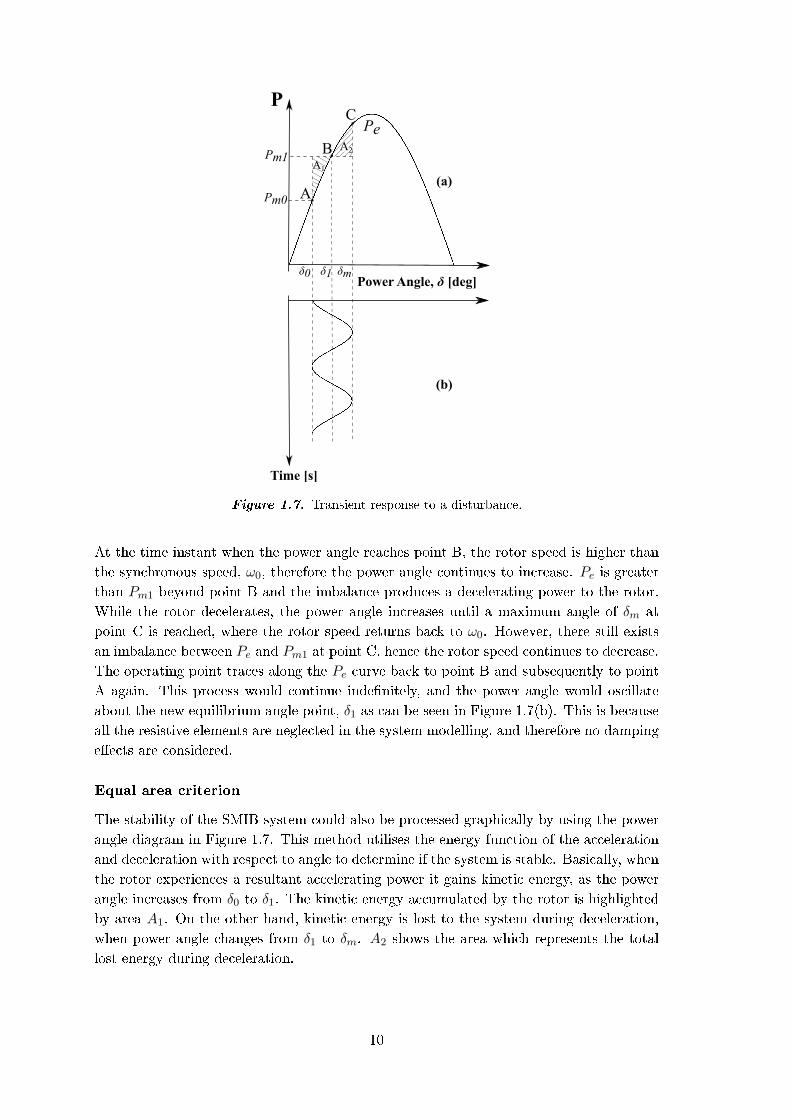
The initial condition of the system is considered to be under steady state operation. Hence,

the initial mechanical power, Pm0 is equal to the electrical output, Pe at point A with a

power angle value of δ0 as shown in Figure 1.7(a). The curve of Pe is determined by the

power-angle relationship established in (1.1).

To study the dynamics of the system, it is subjected to a sudden increase in mechanical

power from Pm0 to Pm1. The new equilibrium point B corresponds to a new power angle

position, δ1. However the power angle can not change immediately owing to the inertia

of the rotor. This results in an imbalance between the mechanical power and electrical

power, and the resultant power is known as accelerating power [2]. This accelerating

power forces the rotor to accelerate, and therefore the power angle increase from point A

to point B along the Pe curve.

9

Power Angle, δ [deg]

P

Time [s]

(a)

(b)

Pm1

δ0 δ1 δm

PeA2

A1

Pm0

C

B

A

Figure 1.7. Transient response to a disturbance.

At the time instant when the power angle reaches point B, the rotor speed is higher than

the synchronous speed, ω0, therefore the power angle continues to increase. Pe is greater

than Pm1 beyond point B and the imbalance produces a decelerating power to the rotor.

While the rotor decelerates, the power angle increases until a maximum angle of δm at

point C is reached, where the rotor speed returns back to ω0. However, there still exists

an imbalance between Pe and Pm1 at point C, hence the rotor speed continues to decrease.

The operating point traces along the Pe curve back to point B and subsequently to point

A again. This process would continue indenitely, and the power angle would oscillate

about the new equilibrium angle point, δ1 as can be seen in Figure 1.7(b). This is because

all the resistive elements are neglected in the system modelling, and therefore no damping

eects are considered.

Equal area criterion

The stability of the SMIB system could also be processed graphically by using the power

angle diagram in Figure 1.7. This method utilises the energy function of the acceleration

and deceleration with respect to angle to determine if the system is stable. Basically, when

the rotor experiences a resultant accelerating power it gains kinetic energy, as the power

angle increases from δ0 to δ1. The kinetic energy accumulated by the rotor is highlighted

by area A1. On the other hand, kinetic energy is lost to the system during deceleration,

when power angle changes from δ1 to δm. A2 shows the area which represents the total

lost energy during deceleration.

10

For the system to be stable, these two areas have to be at least equal or A1 smaller than

A2. If A1 is greater than A2, the system would experience instability as there is insucient

synchronizing torque to stop the increase of the rotor angle and the consequence is loss

of synchronism. If A1 is equal to A2 the system is at its stability limit and δm is the

maximum allowed excursion of δ before instability. The stability criterion is named the

equal area criterion. The mathematical approach used in the criterion is given by (1.3)

which can be deduced from equation (1.2) [2].∫ δm

δ0

(Pm − Pe) dδ = 0 (1.3)

This method presents an alternative to nding the transient stability limit without

having to solve (1.2) using analytical and numerical methods. Though it requires some

modication to be applied to multimachine systems as proposed in [27], it is sucient for

providing an overview on the inuence of elements on transient stability of any system [2].

Critical clearing time (CCT)

Critical clearing time (CCT) is a common stability index used for assessing the transient

stability of a system. It can be dened as the maximum time after fault occurance at which

the fault needs to be cleared without resulting in power angle instability [19]. This is an

important parameter for designing protection systems. As the accuracy of this index is

vital to the system operation coupled with the need to shorten computing time, extensive

research eorts are continuously carried out in this topic [28, 29, 30].

To illustrate the CCT for the SMIB system in Figure 1.5 using the equal area criterion, a

short-circuit fault condition is introduced to the system. Short-circuit on the transmission

line is one of the most common large-disturbances for transient stability analysis. The

considered fault is a three-phase ideal fault located at Line 2, some distance away from

the generator side marked by F in Figure 1.8(a). The equivalent schematic of the faulted

circuit is shown in Figure 1.8(b).

GeneratorInfinite bus

TransformerLine 1

Line 2Fault

FEg EB 0δ

VTXd Xtr

X1

X22

(b)

X21

(a)

Figure 1.8. Graphical representation and schematic of faulted system.

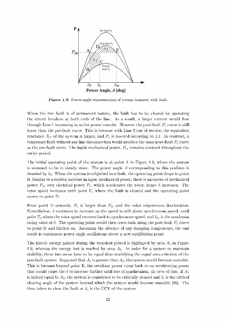
Figure 1.9 shows the power-angle graphical diagram with multiple Pe curves under dierent

network conditions. The pre-fault curve represents power delivered by the generator Pe,

before the fault using (1.1). During fault, the active power delivered will be much less as

compared to before fault. This is because most of the short circuit current will be owing

through inductive reactance to the fault, which causes a reduction in the active power

ow to the innite bus. The power ow is greatly aected by the location of the fault

with respect to the sending end busbar. The closer the fault is to the busbar, the lesser

the active power transfer. An arbitrary curve is chosen to represent Pe during fault.

11

Power Angle, δ [deg]

P

Pm

δ0 δc δm

Pre-fault Pe

A1

D A2A

B

C

E

Post-fault Pe

During-fault Pe

Figure 1.9. Power-angle representation of system transient with fault.

When the line fault is of permanent nature, the fault has to be cleared by operating

the circuit breakers at both ends of the line. As a result, a larger current would ow

through Line 1 increasing in active power transfer. However the post-fault Pe curve is still

lower than the pre-fault curve. This is because with Line 2 out of service, the equivalent

reactance XT of the system is larger, and Pe is lowered according to 1.1. In contrast, a

temporary fault without any line disconnection would produce the same post-fault Pe curve

as the pre-fault curve. The input mechanical power, Pm remains constant throughout the

entire period.

The initial operating point of the system is at point A in Figure 1.9, where the system

is assumed to be in steady state. The power angle, δ corresponding to this position is

denoted by δ0. When the system is subjected to a fault, the operating point drops to point

B. Similar to a sudden increase in input mechanical power, there is an excess of mechanical

power Pm over electrical power Pe, which accelerates the rotor, hence δ increases. The

rotor speed increases until point C, where the fault is cleared and the operating point

moves to point D.

From point D onwards, Pe is larger than Pm and the rotor experiences deceleration.

Nevertheless, δ continues to increase as the speed is still above synchronous speed, until

point E, where the rotor speed recovers back to synchronous speed, and δm is the maximum

swing value of δ. The operating point would then trace back along the post-fault Pe curve

to point D and further on. Assuming the absence of any damping components, the end

result is continuous power angle oscillations about a new equilibrium point.

The kinetic energy gained during the transient period is highligted by area A1 in Figure

1.9, whereas the energy lost is marked by area A2. In order for a system to maintain

stability, these two areas have to be equal thus statisfying the equal area criterion of the

postfault system. Supposed that A1 is greater than A2, the system would become unstable.

This is because beyond point E, the resultant power turns back to an accelerating power

that would cause the δ to increase further until loss of synchronism. In view of that, if A1

is indeed equal to A2, the system is considered to be critically cleared and δc is the critical

clearing angle of the system beyond which the system would become unstable [25]. The

time taken to clear the fault at δc is the CCT of the system.

12

Generally there is no set of values for δc for a single generator as it is dependent on many

factors such as system composition, fault conditions and fault clearance method [21]. For

example, if the post-fault Pe curve is greater, a larger δc is obtained and the CCT would

also increase. Introduction of underground HVAC cables in the system would alter the

overall electrical parameters substantially, in particular the equivalent system reactance

XT in equation (1.1). Thus, the inuence of undergrounding with respect to CCT is

investigated in this thesis.

1.3.2 Multimachine system

A multimachine system is a power system with several interconnected generators in the

network. The stability of the system is not dependent on the individual power angle of

each generator which is measured relative to a rotating reference frame. Instead, the

important factor in this case is the angular separation between generators, which is the

dierence in power angles from one generator to another [25].

Suppose a multimachine system is subjected to a large disturbance resulting in an excess of

accelerating power. All the generators would absorb the majority of the extra power and

begin to accelerate. The simultaneous increase in speed for all generators is acceptable as

long as the power angles are relatively close to one another. The system would eventually

stabilize itself because there is sucient dampening torque in such case [2]. However in

the case where one or more generators is deviating greatly from the rest, after a certain

limit the critical generators would be forced to be disconnected and cause subsequent

disturbance to the system which may lead to instability.

The transient behaviour of the system can be illustrated by using the rubber band analogy

as shown in Figure 1.10 [26]. The weights represent the inertias of the generators and the

rubber band corresponds to the inductance of the transmission lines. The weights are

initially in their equilibrium positions and when one of them is pulled and let go, its

movement would cause an oscillation with the other weights connected by rubber bands.

As a weight is swinging downwards, the rubber band connected to it would stretch as

a result, and this would brake the weights movement and exert a pulling force on the

other weights. The motion would eventually come to a halt depending on the damping

characteristics. If the stress on any rubber band is greater than its strength, it would snap

and the system is no longer intact.

Weight

Rubber band

Figure 1.10. Rubber band analogy for illustration of multimachine power angle stability.

In a large system consisting of many generators, the identication of angular separation

limits is of high complexity [2].

13

It is highly dependant on the location of the disturbance and subsequent power distribution

among the generators determined by the layout of the system. Therefore direct methods

are not used to obtain the CCT of multimachine systems, but instead through iterative

simulations.

1.4 Principles of voltage stability

Following the classications and denitions by the IEEE and CIGRE Taskforce [3], voltage

stability is dened as:

"The ability of a power system to maintain steady voltages at all buses in the system after

being subjected to a disturbance from a given initial operating condition."

The main cause of voltage instability is the inability of the power system to balance

reactive power between generation, lines and loads. Thus, voltage stability is a partial

stability problem which is focused on the behaviour of transmitted power PR, bus voltages

Vi and the reactive power injection Qi at relevant nodes in the system. During a large

disturbance a power system might be exposed to a sudden decrease or increase in reactive

power demands. Such a disturbance could be the loss of generation, line or load, changing

the topology of the system temporarily. Following a disturbance the restoration of loads

can cause stress on the HVAC network by increasing reactive power consumption. Loads

such as induction motors draw increased reactive current during start-up. If the system is

weakened in a post-disturbance condition, due to the disconnection of lines or generation,

it may be pushed beyond its stability limit when exposed to load dynamics. The load

dynamics may attempt to restore power consumption beyond the capability of generation

and the transmission network [3]. For this reason, voltage instability is more likely to

occur when faults are near loads, compared to transient instability, which is more typical

when faults are near generation [3].

If generators are unable to absorb or generate the required reactive power, or if

compensation is insucient, the power system risk a voltage collapse. According to the

authors of [3] a major factor leading to voltage instability is the voltage drop that occurs

due to reactive power ow through inductive reactances of the network. This voltage drop

limits the power transfer capabilities of the system.

The change from OHL to cable based AC transmission is hypothetically particularly

interesting considering large disturbance voltage stability. The reactive power behaviour of

cables is substantially dierent to that of equivalent OHLs, which is elaborated in Section

1.5. Traditionally transmission systems based on OHL require additional reactive power

during a disturbance, in order to raise the voltage and keep it nearer 1 p.u. The extra

reactive power must be supplied by electrical machines, power electronics and switching of

compensation reserves. Synchronous generators have the ability to change their excitation

levels through eld current control. Considering the classical model of synchronous

generators in Figure 1.11, a basic understanding of the reactive power capabilities of

electrical machines can be gained.

14

Rs=0 jXs

Eg δVLN 0Io

Figure 1.11. Classical equivalent circuit of phase (a) for a three-phase synchronous machine.

The stator coil resistance is neglected, Rs = 0.

Eg is often referred to as internal voltage, eld voltage or excitation voltage. The angle

δ is the power angle as explained in Section 1.3. The magnitude of Eg is modelled by a

dependent voltage source, as its value is a function of the eld current If .

The relationship between Eg and If is expressed in equation (1.4), where M is the

mutual inductance linking stator and rotor, assuming a non-salient air-gap, and ωs is

the synchronous speed.

Eg,rms =ωsMIf√

2(1.4)

From the model in Figure 1.11 the apparent three-phase power output So,3ph is expressed

in (1.5), from where the expressions for active and reactive power are derived by taking

the real and imaginary part.

So,3ph = 3VLNI∗o = 3VLN

(Eg − VLNjXs

)∗(1.5)

Po,3ph = Re So,3ph =3VLNEgXs

sin(δ) (1.6)

Qo,3ph = Im So,3ph =3VLNEgXs

cos(δ)−3V 2

LN

Xs(1.7)

Considering both (1.6) and (1.7) it is observed that both active and reactive power are

proportional with the excitation voltage Eg, which can be controlled indirectly through the

eld current Ir [2]. When Qo > 0 the machine is producing reactive power, which is dened

as over-excitation. Decreasing Eg is decreasing Qo, and when Qo < 0 the machine is

absorbing reactive power, which is dened as under-excitation. In other words, regulation

of Eg implies power factor control. Figure 1.12 show how dierent excitation levels aect

the P, δ -characteristics of a synchronous generator. The limit between over- and under-

excitation is arbitrarily displayed in Figure 1.12. In reality this limit is dependent on the

machine design and resulting parameters.

15

Power Angle, δ [deg]

Po [W]

90

(a)

(b)

(c)

Eg,a>Eg,b>Eg,c

Qo>0

Qo<0

Figure 1.12. P, δ-characteristic of a SG with various levels of excitation voltage Eg.

The excitation level of synchronous machines and its eect on the P, δ-curve, indicate

the existing coupling between transient stability and voltage stability. The excitation is

changed in order to respond to a change of reactive power in the power system. Either the

machine is controlled to produce more or less reactive power, or is changed from over- to

under-excited, in response to excessive reactive power in the network. When the machine

excitation is changed drastically, and the P, δ-curve in Figure 1.12 changes from (a) to

(c) or vice versa, the power angle stability limits are inuenced. The consequence may

be power swings similar to the ones presented in Figure 1.7 in Section 1.3. However, now

initiated by a drastic change in reactive power ow.

Reactive power ow and bus voltages are directly related. A simple two bus system with

a generator, line and load is shown in Figure 1.13. The voltage drops from the sending

to the receiving end of the line, due to the ow of current through both resistance and

inductive reactance. Figure 1.14 show the superposition of the voltage drop across the

resistor, and the voltage drop and 90 phase shift due to jX. The resistive voltage drop is

illustrated with real and imaginary part in (a), while the voltage drop of the reactance is

illustrated with real and imaginary part in (b). From Figure 1.14 the sending end voltage

phasor VS can be written as the super position of real and imaginary voltage drops. This

operation is expressed in equation (1.8). Substitution of the expressions in (1.9) into (1.8)

yields equation (1.11), which is the voltage drop equation of the line without capacitance

and conductance to ground. The equation is sometimes presented where δ is assumed

negligible, which eliminates the imaginary part of the expression. The signicance of

(1.11) is the relation between the voltage drop ∆V and reactive power transmitted to the

receiving end QR. The voltage drop is proportional to QR, as transmitting more reactive

power increases the voltage drop across the line. The equation indicate that reactive power

should be supplied locally, rather than transmitted, in order to avoid detrimental voltage

drops throughout the system. It is important to note that there always exist an inevitable

voltage drop due to the line resistance and the transfer of active power.

16

R jX

VR∠0VS∠δ I

PS,QS PR,QR

Figure 1.13. A simple line with impedance Z = R + jX. The current is lagging the voltage

by an angle θ, and δ is the voltage angle at the sending end with reference to the

receiving end.

VS = VR +RI cos(φ) +XI sin(φ) + jXI cos(φ)− jRI sin(φ) (1.8)

PR = VRI cos(φ) and QR = VRI sin(φ) (1.9)

VS = VR +R

VRPR +

X

VRQR + j

X

VRPR − j

R

VRQR (1.10)

∆V = VS − VR = PR

(1

VR

)(R+ jX) +QR

(1

VR

)(X − jR) (1.11)

θ θ

θ

90° inductive phase shift

δ

Vs

VR

I

θVR

RI

RIcos(θ)

-jRIsin(θ)

θ

jXIcos(θ)

XIsin(θ)

jXI

Vs

(a)

(a)

(b)

(b)

RI

jXI

Figure 1.14. Superposition of the voltage drops of a transmission line with line impedance

Z = R + jX. The power factor is lagging, so that the current is lagging the

voltage by θ.

An interesting consideration is the behaviour of cables in the AC transmission system

under large disturbances. Cables in HVAC networks generate large amounts of reactive

power, which is typically compensated by shunt-reactors. During a fault the system

requires injection of reactive power to maintain voltage. Hypothetically the shunt-reactors

of nearby substations could be controlled, or even switched-out, during a fault.

17

As a result the reactive power demand of the system would be decreased, and the HVAC

cables would act as reactive power sources to aid the voltage. Although, an important

note is that the local generation of reactive power will be aected by the drop in voltage.

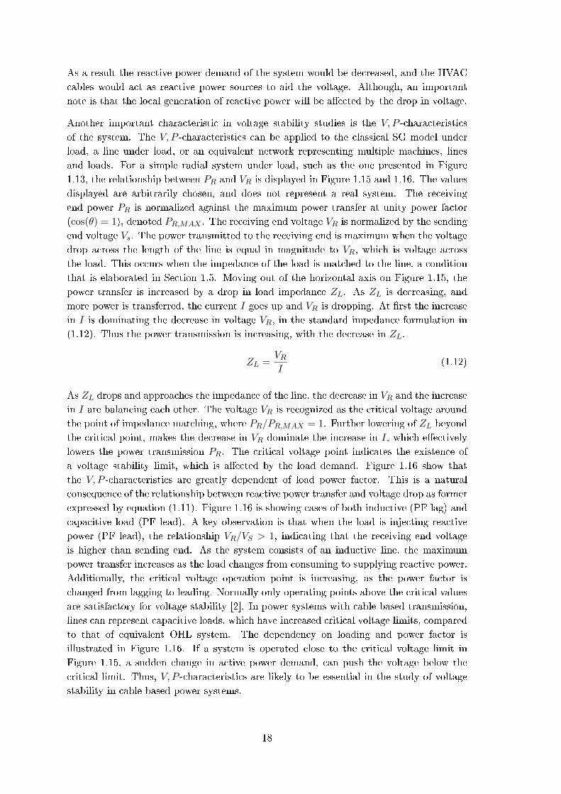
Another important characteristic in voltage stability studies is the V, P -characteristics

of the system. The V, P -characteristics can be applied to the classical SG model under

load, a line under load, or an equivalent network representing multiple machines, lines

and loads. For a simple radial system under load, such as the one presented in Figure

1.13, the relationship between PR and VR is displayed in Figure 1.15 and 1.16. The values

displayed are arbitrarily chosen, and does not represent a real system. The receiving

end power PR is normalized against the maximum power transfer at unity power factor

(cos(θ) = 1), denoted PR,MAX . The receiving end voltage VR is normalized by the sending

end voltage Vs. The power transmitted to the receiving end is maximum when the voltage

drop across the length of the line is equal in magnitude to VR, which is voltage across

the load. This occurs when the impedance of the load is matched to the line, a condition

that is elaborated in Section 1.5. Moving out of the horizontal axis on Figure 1.15, the

power transfer is increased by a drop in load impedance ZL. As ZL is decreasing, and

more power is transferred, the current I goes up and VR is dropping. At rst the increase

in I is dominating the decrease in voltage VR, in the standard impedance formulation in

(1.12). Thus the power transmission is increasing, with the decrease in ZL.

ZL =VRI

(1.12)

As ZL drops and approaches the impedance of the line, the decrease in VR and the increase

in I are balancing each other. The voltage VR is recognized as the critical voltage around

the point of impedance matching, where PR/PR,MAX = 1. Further lowering of ZL beyond

the critical point, makes the decrease in VR dominate the increase in I, which eectively

lowers the power transmission PR. The critical voltage point indicates the existence of

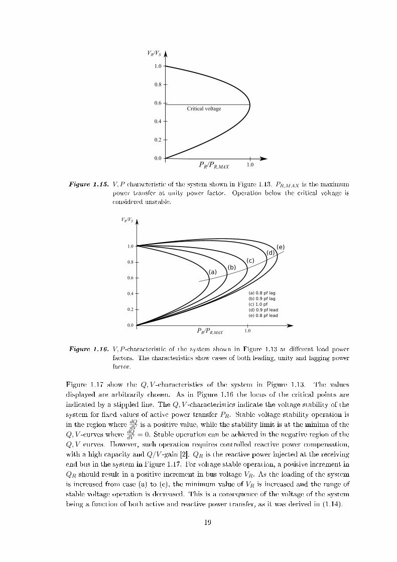
a voltage stability limit, which is aected by the load demand. Figure 1.16 show that

the V, P -characteristics are greatly dependent of load power factor. This is a natural

consequence of the relationship between reactive power transfer and voltage drop as former

expressed by equation (1.11). Figure 1.16 is showing cases of both inductive (PF lag) and

capacitive load (PF lead). A key observation is that when the load is injecting reactive

power (PF lead), the relationship VR/VS > 1, indicating that the receiving end voltage

is higher than sending end. As the system consists of an inductive line, the maximum

power transfer increases as the load changes from consuming to supplying reactive power.

Additionally, the critical voltage operation point is increasing, as the power factor is

changed from lagging to leading. Normally only operating points above the critical values

are satisfactory for voltage stability [2]. In power systems with cable based transmission,

lines can represent capacitive loads, which have increased critical voltage limits, compared

to that of equivalent OHL system. The dependency on loading and power factor is

illustrated in Figure 1.16. If a system is operated close to the critical voltage limit in

Figure 1.15, a sudden change in active power demand, can push the voltage below the

critical limit. Thus, V, P -characteristics are likely to be essential in the study of voltage

stability in cable based power systems.

18

VR/VS

PR/PR,MAX0.0

0.2

0.4

0.6

1.0

1.0

0.8

Critical voltage

Figure 1.15. V, P -characteristic of the system shown in Figure 1.13. PR,MAX is the maximum

power transfer at unity power factor. Operation below the critical voltage is

considered unstable.

VR/VS

PR/PR,MAX0.0

0.2

0.4

0.6

1.0

1.0

0.8

(a)(b)

(c)(d)

(e)

(a) 0.8 pf lag(b) 0.9 pf lag

(d) 0.9 pf lead(e) 0.8 pf lead

(c) 1.0 pf

Figure 1.16. V, P -characteristic of the system shown in Figure 1.13 at dierent load power

factors. The characteristics show cases of both leading, unity and lagging power

factor.

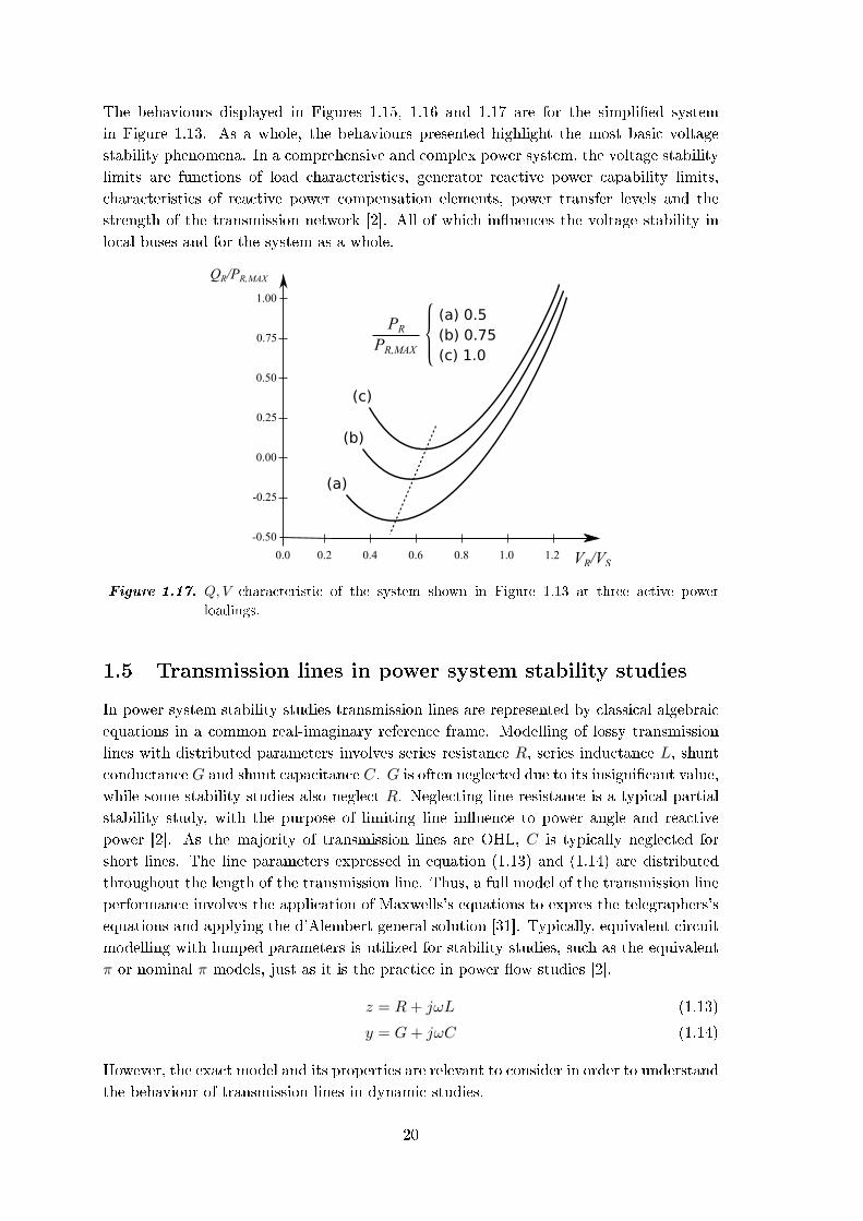
Figure 1.17 show the Q,V -characteristics of the system in Figure 1.13. The values

displayed are arbitrarily chosen. As in Figure 1.16 the locus of the critical points are

indicated by a stippled line. The Q,V -characteristics indicate the voltage stability of the

system for xed values of active power transfer PR. Stable voltage stability operation is

in the region where dQdV is a positive value, while the stability limit is at the minima of the

Q,V -curves where dQdV = 0. Stable operation can be achieved in the negative region of the

Q,V -curves. However, such operation requires controlled reactive power compensation,

with a high capacity and Q/V -gain [2]. QR is the reactive power injected at the receiving

end bus in the system in Figure 1.17. For voltage stable operation, a positive increment in

QR should result in a positive increment in bus voltage VR. As the loading of the system

is increased from case (a) to (c), the minimum value of VR is increased and the range of

stable voltage operation is decreased. This is a consequence of the voltage of the system

being a function of both active and reactive power transfer, as it was derived in (1.14).

19

The behaviours displayed in Figures 1.15, 1.16 and 1.17 are for the simplied system

in Figure 1.13. As a whole, the behaviours presented highlight the most basic voltage

stability phenomena. In a comprehensive and complex power system, the voltage stability

limits are functions of load characteristics, generator reactive power capability limits,

characteristics of reactive power compensation elements, power transfer levels and the

strength of the transmission network [2]. All of which inuences the voltage stability in

local buses and for the system as a whole.

QR/PR,MAX

VR/VS

-0.50

-0.25

0.00

0.25

0.75

1.0

0.50

(a)

(c)

1.00

0.0 0.2 0.4 0.6 0.8 1.2

(b)

PRPR,MAX (c) 1.0

(b) 0.75 (a) 0.5

Figure 1.17. Q,V -characteristic of the system shown in Figure 1.13 at three active power

loadings.

1.5 Transmission lines in power system stability studies

In power system stability studies transmission lines are represented by classical algebraic

equations in a common real-imaginary reference frame. Modelling of lossy transmission

lines with distributed parameters involves series resistance R, series inductance L, shunt

conductance G and shunt capacitance C. G is often neglected due to its insignicant value,

while some stability studies also neglect R. Neglecting line resistance is a typical partial

stability study, with the purpose of limiting line inuence to power angle and reactive

power [2]. As the majority of transmission lines are OHL, C is typically neglected for

short lines. The line parameters expressed in equation (1.13) and (1.14) are distributed

throughout the length of the transmission line. Thus, a full model of the transmission line

performance involves the application of Maxwells's equations to expres the telegraphers's

equations and applying the d'Alembert general solution [31]. Typically, equivalent circuit

modelling with lumped parameters is utilized for stability studies, such as the equivalent

π or nominal π models, just as it is the practice in power ow studies [2].

z = R+ jωL (1.13)

y = G+ jωC (1.14)

However, the exact model and its properties are relevant to consider in order to understand

the behaviour of transmission lines in dynamic studies.

20

An interesting transmission line property following the general solution to telegrapher's

equations is the characteristic impedance Z0. By dening the characteristic impedance as

in equation (1.15) the distributed circuit can simply be represented by the transmission

line (TL) shown in Figure 1.18. Where Z0 express the magnitude of the relationship

between propagating voltage V (z, t) and current I(z, t) at any point z and time t along

the length of the line.

Z0 =

√R+ jωL

G+ jωC(1.15)

Z0

z=0

V++V-

I++I-

ZL

z=l

Figure 1.18. Transmission line representation with forward and backward propagating voltage

V (z, t) and current I(z, t), and characteristic impedance Z0.

If an arbitrary load ZL is impedance matched to Z0, the reection coecients Γv = −Γi =

0, and no reection occurs at the boundary between the line and the load. This principle

is valid at any boundary in the system. The voltage reection coecient is expressed by

equation (1.16).

Γv =V −

V +=ZL − Z0

ZL + Z0(1.16)

If the transmission line is considered lossless, and R = G = 0 in (1.15), the value of Z0 in

(1.15) is reduced to a purely real number, expressed by equation (1.17). As the practical

value of G is close to zero for transmission lines, and R ωL, high-voltage lines are

often assumed to be lossless in dynamic studies. Historically this practice originates from

the study of lightning and switching surges. Thus, the characteristic impedance Z0 of a

lossless line is known as the surge impedance (SI) [2].

Z0 =

√L

C= SI [Ω] (lossless) (1.17)

When a transmission line is loaded by an impedance equal to its SI, the voltage and

current amplitudes are constant along the length l of the line, and the voltage and current

are in phase, resulting in unity power factor. The phase angle between the sending and

the receiving end is δ = 2πlλ , where λ is the wavelength of the travelling wave [2]. The

surge impedance load (SIL) is the power delivered to the SI matching load, and is dened

in equation (1.18).

SIL =V 2LL

Z0[W] (three-phase) (1.18)

So why is surge impedance an important parameter in power system stability? At SIL

the reactive power generated due to the distributed capacitance C, is exactly equal to the

reactive power absorbed, due to the distributed inductance L of the line. This eect can

be realized by observing the current and voltage at any point of the line, showing that

they are in phase.

21

The result is a at voltage prole of the line, meaning no voltage magnitude variation

throughout the total length. Thus, indicating that no reactive power is absorbed or

generated at the ends of the line. For this reason SIL is considered an optimum state

in voltage stability, which is directly related to the control of reactive power and voltage

at specic network points. Hence, SI and SIL are often utilized as a reference values for

transmission lines in voltage stability studies [2].

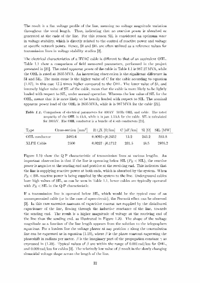
The electrical characteristics of a HVAC cable is dierent to that of an equivalent OHL.

Table 1.1 show a comparison of eld measured parameters, performed in the project

presented in [21]. The rated apparent power of the cable in Table 1.1 is 987.27 MVA, while

the OHL is rated at 2635 MVA. An interesting observation is the signicant dierence in

SI and SIL. The main cause is the higher value of C for the cable according to equation

(1.17), in this case 17.5 times higher compared to the OHL. The lower value of SI, and

inversely higher value of SIL of the cable, mean that the cable is more likely to be lightly

loaded with respect to SIL, under normal operation. Whereas the low value of SIL for the

OHL, means that it is more likely to be heavily loaded with respect to SIL. The nominal

apparent power load of the OHL is 2635 MVA, while it is 987 MVA for the cable [21].

Table 1.1. Comparison of electrical parameters for 400 kV- 50 Hz OHL and cable. The rated

ampacity of the OHL is 4 kA, while it is just 1.5 kA for the cable. SIL is calculated

for 380 kV. The OHL conductor is a bundle of 4 sub-conductors [21].

Type Cross-section[mm2

]R+jX [Ω/km] C [nF/km] SI [Ω] SIL [MW]

OHL conductor 2483.6 0.0092+j0.2452 13.2 243.2 593.8

XLPE Cable 2500 0.0227+j0.1712 231.5 48.5 2976.2

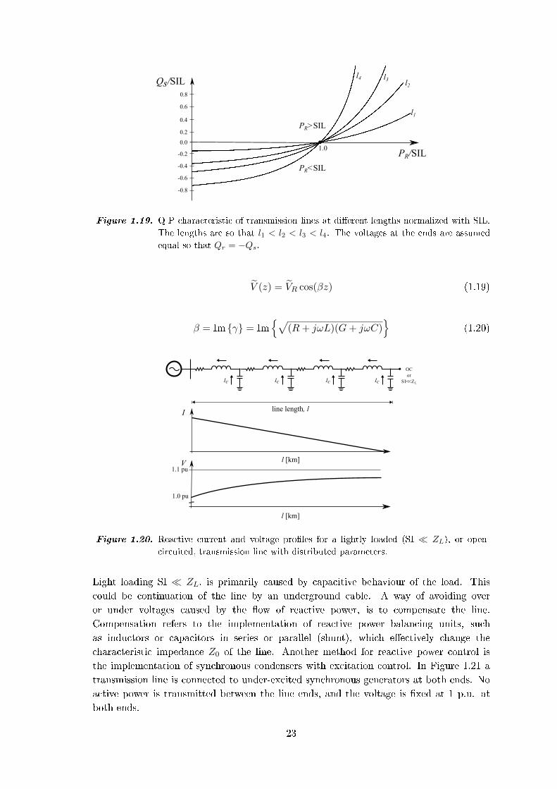
Figure 1.19 show the Q-P characteristic of transmission lines at various lengths. An

important observation is that if the line is operating below SIL (PR < SIL), the reactive

power is negative at the sending end and positive at the receiving end. This indicates that

the line is supplying reactive power at both ends, which is absorbed by the system. When

PR < SIL reactive power is being supplied by the system to the line. Underground cables

have high values of SIL, as can be seen in Table 1.1, hence cables are typically operated

with PR < SIL in the Q-P characteristic.

If a transmission line is operated below SIL, which would be the typical case of an

uncompensated cable (or in the case of open-circuit), the Ferranti eect can be observed

[2]. In this case excessive amounts of capacitive current are supplied by the distributed

capacitance of the line, owing through the inductive reactance of the line, towards

the sending end. The result is a higher magnitude of voltage at the receiving end of

the line than the sending end, as illustrated in Figure 1.20. The shape of the voltage

magnitude as a function of the line length appears from the solution to the telegraphers

equations. For a lossless line the voltage phasor at any position z along the transmission

line can be expressed as in equation (1.19), where β is the phase constant expressing the

phaseshift in radians per meter. β is the imaginary part of the propagation constant γ as

expressed in (1.20). Typical values of β are within the range of 0.001 rad/km for OHL,

and 0.009 rad/km for cables [2]. The relatively low value of β result in the slowly changing

sinusoidal voltage shape across the length of the line.

22

l1

Qs/SIL

PR/SIL1.0

l2

l3 l4

PR<SIL

PR>SIL

-0.2

-0.4

-0.6

-0.8

0.0

0.2

0.4

0.6

0.8

Figure 1.19. Q-P characteristic of transmission lines at dierent lengths normalized with SIL.

The lengths are so that l1 < l2 < l3 < l4. The voltages at the ends are assumed

equal so that Qr = −Qs.

V (z) = VR cos(βz) (1.19)

β = Im γ = Im√

(R+ jωL)(G+ jωC)

(1.20)

line length, l

l [km]

I

l [km]

V

Ic Ic Ic Ic

OCor

SI ZL<<

1.0 pu

1.1 pu

Figure 1.20. Reactive current and voltage proles for a lightly loaded (SI ZL), or open-

circuited, transmission line with distributed parameters.

Light loading SI ZL, is primarily caused by capacitive behaviour of the load. This

could be continuation of the line by an underground cable. A way of avoiding over

or under voltages caused by the ow of reactive power, is to compensate the line.

Compensation refers to the implementation of reactive power balancing units, such

as inductors or capacitors in series or parallel (shunt), which eectively change the

characteristic impedance Z0 of the line. Another method for reactive power control is

the implementation of synchronous condensers with excitation control. In Figure 1.21 a

transmission line is connected to under-excited synchronous generators at both ends. No

active power is transmitted between the line ends, and the voltage is xed at 1 p.u. at

both ends.

23

The gure display how capacitive current is supplied to both ends of the line, implying a

voltage maximum point on the middle of the line. In this conguration the synchronous

condensers are absorbing all the excessive reactive power generated by the transmission

line.

line length, l I

½ l

V

Ic Ic Ic Ic

Vmax

1.0 pu

Figure 1.21. Reactive current and voltage proles for a transmission line connected to external

grids xed at 1 pu voltage. The networks represented at both ends are considered

under-excited, thus absorbing reactive power. No active power are transmitted

from sending to receiving end, Ps = Pr = 0.

Figure 1.22 show a cable with reactive power compensation in the form of shunt reactors

(inductors), located at dierent points. The distributed capacitance C of the cable

produces an excessive amount of capacitive current which must be balanced by the

inductors. The location and size of the inductors inuence the reactive current ow,

and the voltage prole of the cable. Case (a), with compensation at just one line end,

results in the largest reactive current ow and a steeper voltage prole. The reason is

the accumulative reactive current owing through the entire length of the cable. Whereas

the reactive current ow in case (b) and (c) is in both directions, either towards the

ends or towards the middle. By dividing the compensation more evenly throughout the

length of the cable, which is shown in case (d), the reactive current ow in the cable is

limited, resulting in a more at voltage prole. Essentially this brings the characteristic

impedance Z0 of the transmission line closer to impedance matching with the load, and

the cable will display similar characteristics. Sizing and placement of compensation is

not only important in steady state operation and for small-signal stability. In large-

disturbance stability studies the compensation plays an important role with regards to

the initial conditions (post-disturbance) of the stability problem. Likewise, any possible

dynamic compensation will inuence the stability limits during the full duration of the

electromechanical transient.

24

line length, l

I

l [km]

V

Ic Ic Ic Ic Ic

1.0 pu

1.1 pu

100 % 50 % 50 %100 % 25 %25 % 50 %

(a) (b) (c)(d) (b)

(a)(b)(c)

(d) (d)

(d)

Figure 1.22. Reactive current and voltage proles for a cable with distributed parameters and

dierent location and size of inductive shunt compensation. Only the current

magnitudes are shown, however the waveform indicates the direction of ow.

4 cases are shown. (a) 100 % compensation at the sending end, (b) 50 %

compensation at both ends, (c) 100 % compensation at the middle of the cable,

and (d) 50 % compensation on the middle, and 25 % on the ends.

1.6 State of the art review

The following section is a brief review of the latest research and state of the art in stability

studies involving HVAC cables, planning of reactive power and stability indices. The

methodologies and results are discussed, with focus on the applicability and inuence on

the scope of this thesis.

1.6.1 HVAC cables in stability studies

HVAC cables gained traction recently due to growing concerns over the construction of

new high voltage overhead lines. The concerns are related to environmental and landscape

issues. Denmark is one of the few countries that is heading this transition in their

transmission network as described in Section 1.1. As it is not widely adopted yet in

many countries, there is relatively little literature available on stability studies related to

cable systems.

Authors in [19] have made a comparative analysis on transient stability for dierent system

congurations under fault condition. The comparison is done between SMIB systems that

contain cables and with overhead lines only. It is shown in certain cases that the systems

that are made up of uncompensated cables in part of the transmission system display

shorter CCT than the overhead line system. The adverse eect becomes clearer with the

increase of the line length. Figure 1.23 shows the CCT of the investigated systems in [19]

with respect to the length of L2 stretch.

25

L2 is a stretch on the transmission line that was used to carry out the sensitivity analysis.

MLC represents a mixed line system that is made up of both cable and overhead line with

compensation whereas ML is the uncompensated counterpart. OHL denotes the system

in which the line is composed of overhead line only.

Figure 1.23. CCT of investigated systems [19]. System with a higher CCT is more stable.

From Figure 1.23, it can also be observed that compensation helps to improve the stability

of the system. This observation is backed up by studies conducted in [20] and [21]. The

type of stability investigated in [21] includes transient and voltage stability whereas [20]

concentrates on the latter only. The study in [20] is about the voltage stability of an island

grid in Taiwan which is connected to a large grid via submarine cables. Compensation

devices such as static var compensators (SVC) and static synchronous compensators

(STATCOM) are included in the case study as a form of reactive power support. The

disturbance in is the disconnection of one of the cables. The voltage response to the

disturbance of the island grid terminal, Bus 01 for two scenarios is shown in Figure 1.24.

The connection of compensating devices helps to reduce the sudden voltage drop at the

disturbance instance and to restore the voltage level at a much shorter time. In contrast,

the uncompensated system requires the slow acting tap changer on the transformer to

bring the voltage back close to nominal value. The long duration of undervoltage may be

detrimental to the system and components.

Figure 1.24. Voltage response of Bus 01 and Bus 02 when a cable is disconnected at 1 second

[20]. (Left) Without compensators. (Right) With compensators. Bus 01 is the

island grid side terminal of the cable.

26

In addition to fault and disconnection of a line, [21] also covers the connection of a line

as a form of severe disturbance to investigate the transient dynamics of the system in the

presence of cables. The investigation is conducted on the prospective Dutch transmission

network in 2020. The ndings is the same as the one observed in [19] with higher

degree of undergrounding being more vulnerable to instability unless compensated. Figure

1.25 illustrates the voltage transient at the terminal BSL380 during line connection.

Nevertheless, the paper also proposes alternative switching sequences of compensators

to help minimize the eects of voltage variation during line connection and disconnection.

The change is suggested to relief the generators of acting in under-excitation mode for

sustained period of time due to the excess reactive power generated by the cable.

Figure 1.25. BSL380 terminal voltage for dierent degree of cabling during line connection

[21]. Total length of the line is 120 km. OHL and UGC are the abbreviations for

overhead lines and underground cables respectively.

The location of compensators is also of great inuence according to [19] and [21], though

with dierent ndings. The benets of enhancing the system dynamics may outweigh

the extra cost incurred in proper allocation of compensators. The authors in [22]

have presented the idea of utilizing capacitive cables to fully compensate the reactive

power requirement of the overhead lines. This approach may be analytically useful to

provide power correction and result in improved transient stability, however the practical

applicability is limited to a certain extend due to the constraints imposed by political,

environmental and technical feasibility factors.

1.6.2 Planning of reactive power compensation for improved voltage

stability

Following the change from OHL to cable based HVAC transmission, danish TSO

Energinet.dk is implementing reactive power compensation in the form of shunt reactors.

Carsten Rasmussen, Engineer and grid planner, comments on the sizing and positioning

of reactive power in the Danish transmission network:

"The maximum size of the reactors are mainly determined by the maximum allowed

voltage jump when switching the reactors in or out. For screening purposes we use static

calculations (short circuit calculations), where we assume that a voltage jump of 3 % is

OK. If we for instance have a minimum short circuit level, SCL, in a station of 1500 MVA,

then the maximum-size of the reactor is: 1500 MVA · 0.03 = 45 Mvar.

27

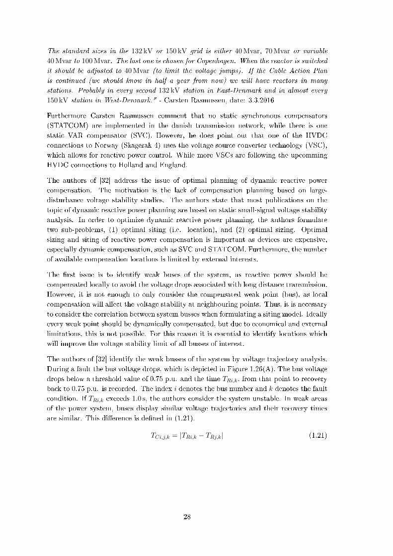
The standard sizes in the 132 kV or 150 kV grid is either 40 Mvar, 70 Mvar or variable

40 Mvar to 100 Mvar. The last one is chosen for Copenhagen. When the reactor is switched

it should be adjusted to 40 Mvar (to limit the voltage jumps). If the Cable Action Plan

is continued (we should know in half a year from now) we will have reactors in many

stations. Probably in every second 132 kV station in East-Denmark and in almost every

150 kV station in West-Denmark." - Carsten Rasmussen, date: 3.3.2016

Furthermore Carsten Rasmussen comment that no static synchronous compensators

(STATCOM) are implemented in the danish transmission network, while there is one

static VAR compensator (SVC). However, he does point out that one of the HVDC

connections to Norway (Skagerak 4) uses the voltage source converter technology (VSC),

which allows for reactive power control. While more VSCs are following the upcomming

HVDC connections to Holland and England.

The authors of [32] address the issue of optimal planning of dynamic reactive power

compensation. The motivation is the lack of compensation planning based on large-

disturbance voltage stability studies. The authors state that most publications on the

topic of dynamic reactive power planning are based on static small-signal voltage stability

analysis. In order to optimize dynamic reactive power planning, the authors formulate

two sub-problems, (1) optimal siting (i.e. location), and (2) optimal sizing. Optimal

sizing and siting of reactive power compensation is important as devices are expensive,

especially dynamic compensation, such as SVC and STATCOM. Furthermore, the number

of available compensation locations is limited by external interests.

The rst issue is to identify weak buses of the system, as reactive power should be

compensated locally to avoid the voltage drops associated with long distance transmission.

However, it is not enough to only consider the compensated weak point (bus), as local

compensation will aect the voltage stability at neighbouring points. Thus, it is necessary

to consider the correlation between system busses when formulating a siting model. Ideally

every weak point should be dynamically compensated, but due to economical and external

limitations, this is not possible. For this reason it is essential to identify locations which

will improve the voltage stability limit of all busses of interest.

The authors of [32] identify the weak busses of the system by voltage trajectory analysis.

During a fault the bus voltage drops, which is depicted in Figure 1.26(A). The bus voltage

drops below a threshold value of 0.75 p.u. and the time TRi,k, from that point to recovery

back to 0.75 p.u. is recorded. The index i denotes the bus number and k denotes the fault

condition. If TRi,k exceeds 1.0 s, the authors consider the system unstable. In weak areas

of the power system, buses display similar voltage trajectories and their recovery times

are similar. This dierence is dened in (1.21).

TCi,j,k = |TRi,k − TRj,k| (1.21)

28

Figure 1.26. Bus voltage trajectories in response to a fault. In (A) the voltage is able to recover

above the threshold value, while it is unable in (B). The threshold value of 0.75

p.u. is indicated by the dashed line. [32]

In some cases the voltage cannot recover to the threshold voltage of 0.75 p.u. This is

depicted in Figure 1.26(B). In this case the recovery time is dened as in equation (1.22),

where Tm is a xed large recovery time of 10 s, T1 is the incident time of the fault, Tmaxis the time of maximum recovery voltage post fault, and Umax is the maximum post fault

voltage.

TRi,k = Tm + (1− Umax) · (Tmax − T1) (1.22)

Based on simulations the recovery times TRi,k of weak buses are recorded and stored in a

matrix T in (1.23). The row number m is the specic weak bus, while the column number

n is the fault type.

T =

TR1,1 TR1,2 · · · TR1,n

TR2,1 TR2,2 · · · TR2,n...

.... . .

...

TRm,1 TRm,2 · · · TRm,n

(1.23)

The authors of [32] use the voltage trajectory analysis to perform an optimization of

size and location of reactive power compensation. In short, their proposed method

optimizes the reactive power compensation by identifying the most improved voltage

trajectories according to the denitions. It is concluded that the method proposed provides

a ecient way of planning reactive power compensation based on large disturbance voltage

stability. It is highlighted how the compensation at one bus will aect other buses, and

how the method secures that the individual bus is neither over compensated nor under

compensated.

1.6.3 Stability indices for transient and voltage stability analysis

Choosing an appropriate stability index for assessment of power system stability is essential

in stability analysis. Firstly, the index should be relevant according to the questioned

instability type. Whether it is a transient stability or voltage stability problem, or even

a specic sub-type as categorized in [3] and presented in Figure 1.2. Secondly the index

and the associated methodology should be suitable for the scope of the analysis. Overall,

power system stability can be assessed in two dierent ways. Either from a mathematical

stability theoretical approach, or from what in [3] is referred to as the practitioners way.

The power system practitioner asses the stability through software simulations.

29

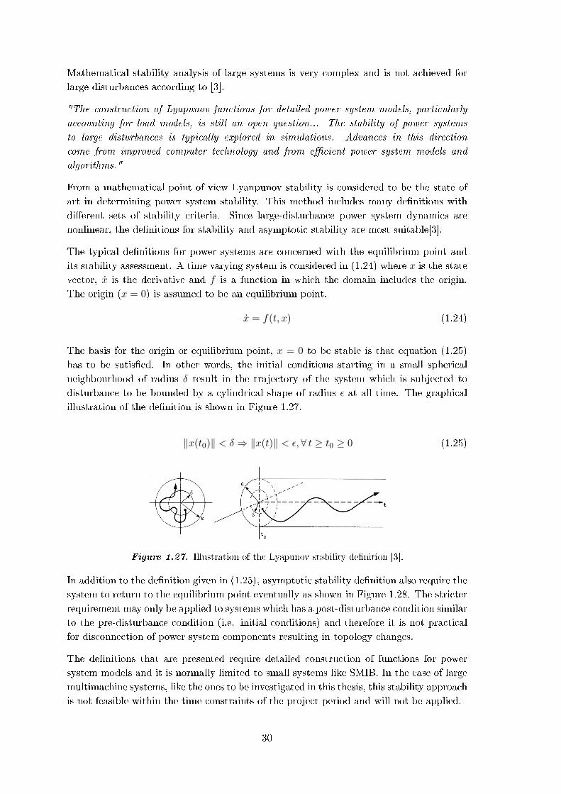
Mathematical stability analysis of large systems is very complex and is not achieved for

large disturbances according to [3].

"The construction of Lyapunov functions for detailed power system models, particularly

accounting for load models, is still an open question... The stability of power systems

to large disturbances is typically explored in simulations. Advances in this direction

come from improved computer technology and from ecient power system models and

algorithms."

From a mathematical point of view Lyanpunov stability is considered to be the state of

art in determining power system stability. This method includes many denitions with

dierent sets of stability criteria. Since large-disturbance power system dynamics are

nonlinear, the denitions for stability and asymptotic stability are most suitable[3].

The typical denitions for power systems are concerned with the equilibrium point and

its stability assessment. A time varying system is considered in (1.24) where x is the state

vector, x is the derivative and f is a function in which the domain includes the origin.

The origin (x = 0) is assumed to be an equilibrium point.

x = f(t, x) (1.24)

The basis for the origin or equilibrium point, x = 0 to be stable is that equation (1.25)

has to be satised. In other words, the initial conditions starting in a small spherical

neighbourhood of radius δ result in the trajectory of the system which is subjected to

disturbance to be bounded by a cylindrical shape of radius ε at all time. The graphical

illustration of the denition is shown in Figure 1.27.

‖x(t0)‖ < δ ⇒ ‖x(t)‖ < ε,∀ t ≥ t0 ≥ 0 (1.25)

Figure 1.27. Illustration of the Lyapunov stability denition [3].

In addition to the denition given in (1.25), asymptotic stability denition also require the

system to return to the equilibrium point eventually as shown in Figure 1.28. The stricter

requirement may only be applied to systems which has a post-disturbance condition similar

to the pre-disturbance condition (i.e. initial conditions) and therefore it is not practical

for disconnection of power system components resulting in topology changes.

The denitions that are presented require detailed construction of functions for power

system models and it is normally limited to small systems like SMIB. In the case of large

multimachine systems, like the ones to be investigated in this thesis, this stability approach

is not feasible within the time constraints of the project period and will not be applied.

30

Figure 1.28. Illustration of Lyapunov asymptotic stability denition [3].

In this thesis both transient stability and large-disturbance voltage stability is to be

analysed. This is done for systems larger than the SMIB system, more specically the

IEEE 9-bys system and IEEE 39-bus system. Thus stability indices, which are suitable

for large system analysis are to be chosen, for both partial stability problems.

In transient stability the parameters of interest are mainly the active power transmission

and power angle, (P, δ)-characteristics. The most used index for transient stability is the

critical clearing time (CCT), which is elaborated in Section (1.3.1). CCT can be assessed

both mathematically and by simulations. Through simulations the CCT can be obtained

by iterative sensitivities of the system.

For voltage stability studies the choice of stability index is not as straight forward. The

author of [2] comments on stability margins and indices of voltage stability: "There are at

present no widely accepted guidelines for selection of the degree of margin and the system

parameters to be used as indices. These are likely to be system dependent and may have

to be established based on the characteristics of the individual system."

The work in [2] was published in year 1993, but as of today indices for voltage stability is

still a research topic.

Voltage stability is concerned with the parameters V , P and Q at critical nodes of the

system. Thus assessing voltage stability by CCT, which is associated with the power angle

δ, is an indirect way of analysing voltage stability. Recent voltage stability studies utilize a

form of simulation based trajectory analysis for analysing instabilties [20]. However, other

studies are still based on determining δ, even if the topic is compensation of voltage by

reactive power [22]. Thus, no general consensus regarding the use of voltage stability index

exist. For small-signal voltage stability several alternative indices have been used. The

authors of [33] compare and discuss previous methods and propose a new index. However,

the methods are focused on the voltage collapse following small-signal load variations, and

have not been veried for large disturbances.

The authors of [34] discuss the advantages and disadvantages of large-disturbance

stability indices, while proposing a new method. In papers [32] and [21] the large-

disturbance voltage stability is assessed by evaluating voltage waveforms in dierent

dynamic situations. The eect of reactive power compensation is analysed directly by

observation of v(t) following a large disturbance, and doing incremental ∂v(t)∂Q ≈ ∆v

∆Q

sensitivities. This method is simple, but has the disadvantage of not providing a qualitative

denition of stability margins.

31

1.6.4 Evaluation criteria of large-disturbance voltage trajectories

As it was discussed in Section 1.6.3, there is no standard method for assessment of voltage

stability for large-disturbances. In this thesis a voltage trajectory method similar to the

one presented in [32], and discussed in Section 1.6.2, is to be utilized for comparison

of OHL and cable based networks. Voltage trajectory analysis is considered a simple

method for comparing dierent cases of system topology with respect to voltage stability

performance. However, a disadvantage of the method is that it does not assess the voltage

stability margin, and the so called distance to instability. Thus, the method is not suited

for determining if an actual case will lead to instability, but rather for comparing and

determining whether a given case has an improving or decreasing eect on voltage stability.

Following a large disturbance, the voltage trajectory (i.e. voltage waveform) at a given

node in the power system, will display certain characteristics. Here the focus is on

the power systems ability to recover local voltages within a certain time frame. Thus,

observing the voltage trajectory, the important parameters are the voltage recovery time

tR from the incident of the disturbance, to a voltage above a certain threshold, and the

recovery voltage vR.

In this thesis, it is decided to evaluate the voltage trajectories against an under-voltage

limit provided by Nan Qin, Ph.d. student and employee at danish TSO Energinet.dk.

The under-voltage limit is displayed in Figure 1.29. The original gure is published in

[35], displaying both under-voltage and over-voltage limits.

0 1 2 3 4 5 6 7 8 9 10 11 12

Time, t [s]

0

0.2

0.4

0.6

0.8

1

Vol

tage

in p

.u.

Voltage limit

Figure 1.29. Under-voltage limits following large-disturbances for assessing voltage stability

[35].

The under-voltage limit is not part of a grid-code, but is an evaluation criterion used to

assess voltage stability under large disturbances. It is used to assess the voltage prole at

any node in the transmission grid, and it considers protection and operational limits of

the system and equipment.

32

The under-voltage limit displayed in Figure 1.29 dictates that in order to consider voltage

stable operation, the voltage should be able to recover to atleast 0.75 p.u. within 1 s of

clearing the disturbance. Thus, the minimum slope of recovery from 0.25 p.u. to 0.75

p.u. should be ∆V/∆t = 0.5. Furthermore, 10 s after clearing the disturbance the voltage

should have recovery to more than 0.90 p.u.

If the voltage trajectory of any node following a disturbance, does not satisfy these limits

in the given time, the continuous operation at the specic node cannot be guaranteed.

Consequences of under-voltage operation may be increased current drawn by constant

power loads and stalling of induction motors, which may further detriment the system

voltage. Under-voltage load shedding and tripping of under-voltage protection may be a

necessary resort to avoid a system collapse.

33

Problem statement andmethodology 2

This chapter lists the problem statement of the thesis together with the specic objectives

realized to answer the problem. The delimitation of the thesis scope is described together

with the chosen methodology.

2.1 Problem statement

Danish TSO Energinet.dk is in the process of undergrounding parts of the AC

transmission grid in Denmark. The aected voltage levels range from 132 kV to

400 kV. Undergrounding involves the replacement of conventional OHL transmission with

underground cables. A major dierence in terms of electrical parameters is that cables

are mainly capacitive and a source of reactive power, in contrast to the inductive OHL,

that absorbs reactive power due to typical operation above SIL.

The focus of this thesis is to study the electromechanical dynamics associated with the

implementation of long HVAC cables in the power transmission network. The main

objective is to assess and study the transient stability and large-disturbance voltage

stability of generic power systems. The analysis is to be initiated on a simple single-

machine innite bus system, and then expanded to IEEE 9-bus system and IEEE 39-bus

multi machine systems. The stability of power systems with OHL and cable based HVAC

transmission is to be compared through sensitivity studies of fault duration, fault location,

reactive power compensation degrees, load levels and more.

Transient stability studies are to be performed with critical clearing time (CCT) as index

for power angle stability assessment.

In the case of voltage stability, V, P and Q,V -characteristics are used as static indices

for comparing the performance of the two dierent systems. It is to be investigated how

varying the degree of reactive power compensation can inuence the steady state stability

performance.

The dynamic large-disturbance voltage stability is to be assessed by observing voltage

trajectories at load buses following a series of large-disturbance events. The analysis is

focused on the eects of dynamic switching of compensation devices (i.e. shunt reactors)

on the voltage trajectory.

The questions to be answered are: Does undergrounding of HVAC transmission networks

inuence the transient and voltage stability limits of power systems? How can the stability

be improved by utilizing reactive power compensation?

35

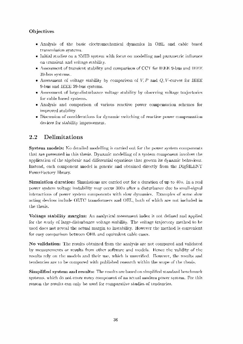
Objectives

Analysis of the basic electromechanical dynamics in OHL and cable based

transmission systems.

Initial studies on a SMIB system with focus on modelling and parametric inuence

on transient and voltage stability.

Assessment of transient stability and comparison of CCT for IEEE 9-bus and IEEE

39-bus systems..

Assessment of voltage stability by comparison of V, P and Q,V -curves for IEEE

9-bus and IEEE 39-bus systems.

Assessment of large-disturbance voltage stability by observing voltage trajectories

for cable based systems.

Analysis and comparison of various reactive power compensation schemes for

improved stability.

Discussion of considerations for dynamic switching of reactive power compensation

devices for stability improvement.

2.2 Delimitations

System models: No detailed modelling is carried out for the power system components

that are presented in this thesis. Dynamic modelling of a system component involves the

application of the algebraic and dierential equations that govern its dynamic behaviour.

Instead, each component model is generic and obtained directly from the DIgSILENT

PowerFactory library.

Simulation duration: Simulations are carried out for a duration of up to 40 s. In a real

power system voltage instability may occur 300 s after a disturbance due to small-signal

interactions of power system components with slow dynamics. Examples of some slow

acting devices include OLTC transformers and OEL, both of which are not included in

the thesis.

Voltage stability margins: An analytical assessment index is not dened and applied

for the study of large-disturbance voltage stability. The voltage trajectory method to be

used does not reveal the actual margin to instability. However the method is convenient

for easy comparison between OHL and equivalent cable cases.

No validation: The results obtained from the analysis are not compared and validated

by measurements or results from other software and models. Hence the validity of the

results rely on the models and their use, which is unveried. However, the results and

tendencies are to be compared with published research within the scope of the thesis.

Simplied system and results: The results are based on simplied standard benchmark

systems, which do not cover every component of an actual modern power system. For this

reason the results can only be used for comparative studies of tendencies.

36

2.3 Methodology

Software and models: DIgSILENT PowerFactory is the software used for performing

all necessary simulations of the project. An SMIB model is constructed by connecting

the respective elements found in the software. In this software the basic tap and load

ow data of the elements need to be dened for power ow solutions. As in the case of

9-bus and 39-bus systems, both models are taken from the examples given in this software.

Additionally Matlab is used to process the results exported from PowerFactory and to plot

gures presented in the thesis.

Simulations: Dynamic RMS simulations are carried out to obtain the critical clearing

time and voltage trajectory of the systems. Simulation events are dened to initiate

disturbances and SR-switching. A DPL script is also used to automate the clearing time

increment during simulations in order to determine the critical clearing time. Meanwhile,

load ow calculations are performed in steady state analysis from which the V, P and Q,V -

characteristic curves are obtained. The short-circuit power of each bus in the network can

be computed using short-circuit calculations command in the software.

Result analysis: Results from simulations are compared and analysed based on

theoretical principles. In the transient stability study, the focus is on interpreting the

tendencies displayed by the CCT values from varying line parameters and compensation

schemes. As for voltage stability, the voltage trajectories are used to illustrate

considerations for dynamic SR-switching.

37

Stability analysis ofsingle-machine infinite bus

system 3This chapter is an introduction to the transient and voltage stability analysis presented

in this thesis. It is an initial comparison of OHL and cables in stability studies, with

focus on their parametric dierences. The purpose is to illustrate and highlight the main

electromechanical dynamics and present those in a simplistic and clear way. A single-

machine innite bus system is used for the analysis which is performed using DIgSILENT

PowerFactory.

A discussion of the inuence of transmission line capacitance on the classical P, δ -equation

for a SMIB system is located in Appendix A.

3.1 Single-machine innite bus system

The single-machine innite bus system (SMIB) is described in Section 1.3.1, and

reproduced in Figure 3.1 for convenience. The SMIB system is widely used in stability

studies for its simplicity, especially when a mathematical approach is desired. The innite

bus is characterized by a constant voltage at constant frequency, regardless of active and

reactive power ow. In reality innite buses do not exist, and does not represent a real

power system with electromechanical dynamics. However, with a xed frequency (e.g. 50

Hz), the innite bus is providing a convenient reference frame for the display of bus angles

for the study of stability in simplied cases. The purpose of the parallel line conguration

is for the two ends of the transmission system to maintain connection during and after a

large disturbance in Figure 3.1(B).

IB

Xl1

Xl2

VB

SG

IBXl

VBSG

(A)

(B)

Figure 3.1. (A) Single-line diagram SMIB with one line connecting the electrical machine to

the innite bus, and (B) two parallel and equal lines connecting the two ends.

39

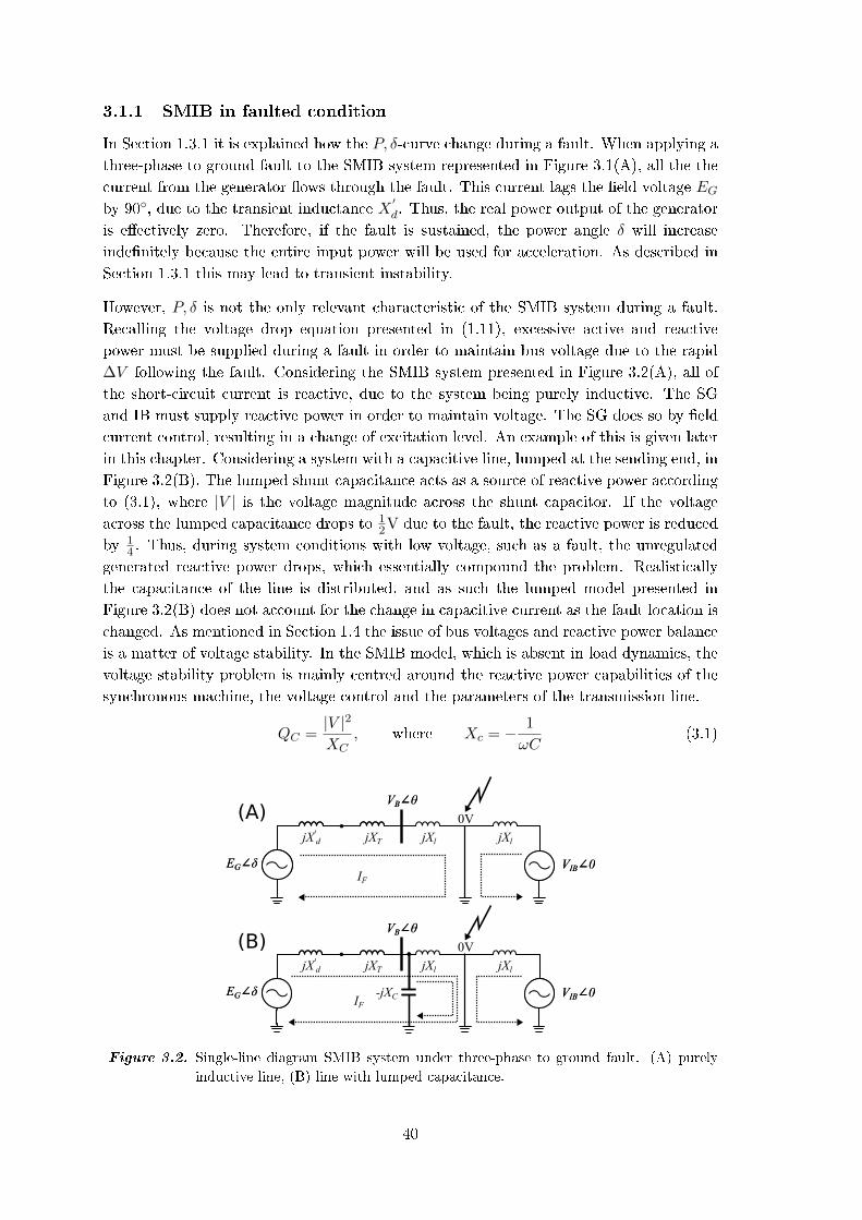
3.1.1 SMIB in faulted condition

In Section 1.3.1 it is explained how the P, δ-curve change during a fault. When applying a

three-phase to ground fault to the SMIB system represented in Figure 3.1(A), all the the

current from the generator ows through the fault. This current lags the eld voltage EGby 90, due to the transient inductance X

′d. Thus, the real power output of the generator

is eectively zero. Therefore, if the fault is sustained, the power angle δ will increase

indenitely because the entire input power will be used for acceleration. As described in

Section 1.3.1 this may lead to transient instability.

However, P, δ is not the only relevant characteristic of the SMIB system during a fault.

Recalling the voltage drop equation presented in (1.11), excessive active and reactive

power must be supplied during a fault in order to maintain bus voltage due to the rapid

∆V following the fault. Considering the SMIB system presented in Figure 3.2(A), all of

the short-circuit current is reactive, due to the system being purely inductive. The SG

and IB must supply reactive power in order to maintain voltage. The SG does so by eld

current control, resulting in a change of excitation level. An example of this is given later

in this chapter. Considering a system with a capacitive line, lumped at the sending end, in

Figure 3.2(B). The lumped shunt capacitance acts as a source of reactive power according

to (3.1), where |V | is the voltage magnitude across the shunt capacitor. If the voltage

across the lumped capacitance drops to 12V due to the fault, the reactive power is reduced

by 14 . Thus, during system conditions with low voltage, such as a fault, the unregulated

generated reactive power drops, which essentially compound the problem. Realistically

the capacitance of the line is distributed, and as such the lumped model presented in

Figure 3.2(B) does not account for the change in capacitive current as the fault location is

changed. As mentioned in Section 1.4 the issue of bus voltages and reactive power balance

is a matter of voltage stability. In the SMIB model, which is absent in load dynamics, the

voltage stability problem is mainly centred around the reactive power capabilities of the

synchronous machine, the voltage control and the parameters of the transmission line.

QC =|V |2

XC, where Xc = − 1

ωC(3.1)

VB∠θ

VIB∠0EG∠δ

VB∠θ

VIB∠0EG∠δ

jX'd jXT jXljXl

0V

IF

VB∠θ

VIB∠0EG∠δ

VB∠θ

VIB∠0EG∠δ

jX'd jXT jXljXl

0V

-jXCIF

(A)

(B)

Figure 3.2. Single-line diagram SMIB system under three-phase to ground fault. (A) purely

inductive line, (B) line with lumped capacitance.

40

3.2 Introducing the DIgSILENT PowerFactory SMIB

system

In order to analyse the dynamic behaviour of the SMIB system it is modelled using

DIgSILENT PowerFactory version 15.1.6. The SMIB system is constructed with two

parallel lines, as displayed in Figure 3.3. The system frequency is 50 Hz. The components

of the system are the following:

(A) DIgSILENT standard model synchronous machine. Nominal apparent power:

255 MVA. Nominal voltage: 19 kV. Transient reactance, X′d = 0.21 p.u. Inertia

constant, H = 10 s.

(B) 2-Winding 19/220 kV Transformer. Y-Y connected, with both neutrals grounded.

Rated apparent power: 500 MVA. Leakage reactance XT = 0.5 p.u.

(C) Line 1: Lumped parameter nominal pi modelled line. Length, l = 100 km. Initially

lossless, R = G = 0. RMS-simulation applies a three-phase fault at tf,0 = 0.1 s at

a distance df from the sending end bus BB1. The fault is cleared by opening the

line at both ends at tc, so that the time under which the SMIB system is faulted is

tf = tc − tf,0.(D) Line 2: Lumped parameter nominal pi modelled line. Line parameters and length

are exactly equivalent to those of Line 1 (C). This line is not faulted, and remains

in service in any operation condition.

(E) External grid acting as innite bus. The voltage is 1 p.u. in steady state and acts as

angle reference xed at 0. The external grid is not an ideal voltage source. Thus,

it is not able to keep the voltage at 1 p.u, and the frequency at 50 Hz during a fault.

However, it resembles a strong grid with a short-circuit power of 10 000 MVA.

Figure 3.3. Single-line diagram of the SMIB system modelled in DIgSILENT PowerFactory.

The markings (A) through (E) indicate the components listed.

3.2.1 Synchronous machine controls in PowerFactory

In PowerFactory v. 15.1.6 the synchronous machine can be modelled as either voltage

controlled or power factor controlled. As stated in DIgSILENT documentation [36] the

voltage controlled mode is the typical setting for large synchronous generators. Thus,

voltage controlled mode is used for the results presented, unless it is desired to force the

reactive power output of the generator to highlight certain dynamics. In such case, the

use of power factor control will be stated explicitly.

41

The Local Controller dened as "Const. V" is typically used for large synchronous

generators at large power stations which operate in voltage control mode ("PV" mode).

When enabling this option, the generator will control the voltage directly at its terminals.

As basis for the controlled [p:u:] value, the voltage of the connected terminal is used.

The Local Controller dened as "Const. Q" is typically used for smaller synchronous

generators, like the ones embedded in distribution grids, where the power factor is keep

constant ("PQ" mode). With this type of control, the user can specify the active and

reactive power dispatch of the generator.

Besides the choice of local controller, various plant models can be added to the synchronous

machine. The three main control systems are:

Automatic voltage regulator (AVR), also referred to as excitation system. The

purpose of the AVR is to adjust the generator eld current to maintain a constant

terminal voltage.

Governor: Used to control the generator speed, helping to maintain a desired

frequency.

Power System Stabilizer (PSS): The purpose of the PSS is to add a signal to the

excitation system proportional to shaft speed deviation, and electrical power in case

of dual input stabilizer. This adds dampening to the power oscillations following a

large disturbance.

A discussion of the impact of the dierent machine controls is located in Appendix B. The

SMIB results presented in this chapter are produced with AVR as the only added control.

The argument is that AVR is the most relevant control in the study of large-disturbance

stability and the regulation of voltage and reactive power with respect to line parameters

and compensation.

3.2.2 Increasing the duration of the fault

Increasing the time under which the SMIB system is faulted tf , will aect the transient

response of the system. In Section 1.3.1 it is described how the swing equation governs the

power angle oscillations in response to a fault. If the power angle exceeds a critical value

during a fault the machine becomes unstable, unless the fault is cleared before reaching

this limit. Figure 3.4 displays how the power angle oscillations increase as a consequence of

increased fault duration. When tf is increased the amplitude of the oscillations increases.

The power angle reaches a higher value in the post-fault state, before the rotor speed

recovers back to synchronous speed. This concept is further explained in Section 1.3.1

Figure 1.9. In all the cases displayed the SMIB system is stable as it recovers to steady

state. However, the post-fault steady state power angle is increased compared to the pre-

fault value, as the faulted line is taken out of service, resulting in an increased system

reactance.

42

0 0.5 1 1.5 2 2.5 3 3.5 4 4.5 5

Time, t [s]

-20

0

20

40

60

80

100

120

Pow

er A

ngle

, δ [d

eg]

tf = 0.1 s

tf = 0.2 s

tf = 0.3 s

tf = 0.4 s

tf = 0.5 s

Figure 3.4. Power angle fault response of the SMIB system, as a result of a fault at tf,0 = 0.1 s.

The duration of the fault is increased from 0.1 s to 0.5 s.

3.2.3 Obtaining the CCT in PowerFactory

As tf is increased the system is approaching its transient stability limit. The maximum

permissible tf for stable operation was dened as CCT in Section 1.3.1. In order to

evaluate CCT in PowerFactory a transient stability limit must be dened to enable

the detection of instability. DIgSILENT PowerFactory has a built-in function to detect

whether an electrical machine has lost synchronism. The function is referred to as out

of step detection or "pole-slip" in the DIgSILENT manual. Initially this method is used

to evaluate CCT for transient stability studies in this thesis. However, after experiencing

examples of inconsistency in the method and results, the evaluation of CCT by the pole-

slip function is discontinued. A description of the pole-slip method is located in Appendix

E together with a discussion of the inconsistencies which are discovered.

Instead a xed power angle limit δlim is set. If the power angle δ reaches δlim, the machine

is considered unstable. In [2] it is stated that 90 is considered the nominal limiting value

for a two machine system. However, in [2] the following is emphasized: "Limiting values

of power transfers and angular separation are a complex function of generation and load

distribution." Thus, δlim is dependent on the network topology and the transmission of

active and reactive power. In this thesis δlim is chosen at 180 separation, as acceleration

beyond this angle theoretically implies that the electrical machine changes from a generator

to a motor. δlim should not be confused with the critical clearing angle. The critical

clearing angle is the maximum allowed angular separation at the time of fault clearing,

whereas δm is the maximum angle reached after clearing. When the fault is cleared the

machine continues to accelerate till it reaches δm.

Having dened δlim = 180 , the CCT becomes the maximum allowed clearing time

tc, which ensures that the power angle separation never reaches or exceeds 180. In

order to assess CCT for the SMIB system in PowerFactory a simple DPL (DIgSILENT

Programming Language) script is executed. The DPL script runs a for-loop, which

performs RMS simulations while increasing the clearing time tc, and thus the fault duration

tf . This procedure is iterated until δm ≥ 180 , and the fault duration tf reached in that

iteration is the CCT. The DPL code used is located in Appendix D.

43

It can be argued that the choice of δlim = 180 is weakly motivated, as it is chosen without

consideration of machine parameters and initial conditions of the system. Undoubtedly

the method introduces a large uncertainty to the actual CCT values obtained. However,

the purpose of this thesis is to compare generic OHL and cable based networks, and

study the tendencies and sensitivities of line parameters. Thus, the dierences in system

behaviour are more relevant than the actual values obtained.

3.3 Sensitivity study of line parameters on the SMIB

system

Now, sensitivity studies of the line parameters L, C and R are performed on the SMIB

system in PowerFactory. Studies of shunt conductance G are not performed, due to its

typically negligible value. When a parameter is changed, it is done to both parallel lines

simultaneously, so that they are always equal. Variations in power angle response and

CCT are presented to study the impact on transient stability, while voltage and reactive

power trajectories are displayed for the study of voltage stability.

3.3.1 Sensitivity of transmission line inductance

The transmission lines of the SMIB system are initially chosen to be purely inductive.

The rst step of the line parameter sensitivity study is to investigate the inuence of

increasing Xl. Figure 3.5 show how the CCT is decreased as the reactance of the line is

increasing. Two cases are displayed, one where the fault is at the sending end df = 1 km,

and one where the fault is at the receiving end df = 99 km. The CCT is longer if the fault

is located at the receiving end of the system. In other words, the system is more stable

for faults farther away. Both SG and IB supplies reactive power to the fault, but as the

distance to the fault is increased, less reactive short-circuit current from the SG will be

transfered through the purely inductive faulted line. When the fault is located at 99 km

from the SG bus, the reactance of the fault loop, illustrated in Figure 3.2, is signicantly

bigger than when it is at 1 km. This is simply due to the total line impedance being a

linear function of the length:

Zl = (R+ jωL)l [Ω] (3.2)

The SG has nite short-circuit capability, and if less reactive power is supplied to the

fault, more active power can be transferred to the IB on the healthy parallel line. In

other words the P, δ-curve of the generator does not drop to zero during the fault, and

it is able to supply active power to the IB. Recalling Figure 1.9, this results in a steeper

P, δ-characteristic during the fault. As it is explained in Section 1.3.1, the shape of the

P, δ curve is directly inuencing the kinetic energy areas A1 and A2. When the fault is

far away, df = 99 km, the kinetic energy gained due to acceleration A1 is smaller, due to

the steeper P, δ-curve during the fault. The equal area criterion states that if A1 > A2,

the system becomes unstable.

44

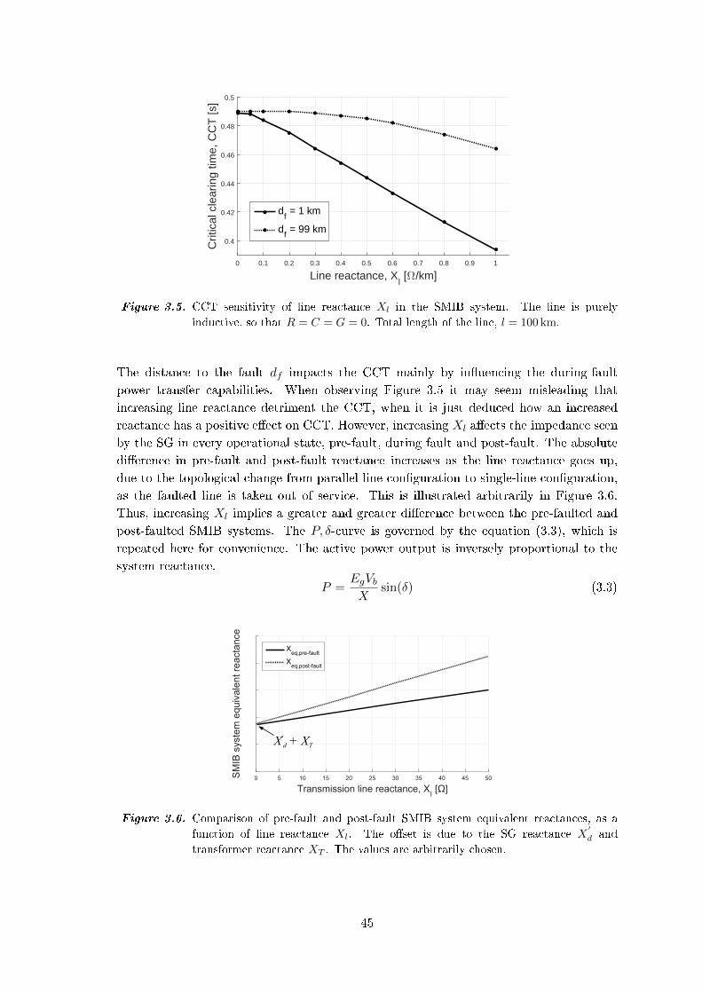
0 0.1 0.2 0.3 0.4 0.5 0.6 0.7 0.8 0.9 1

Line reactance, Xl [Ω/km]

0.4

0.42

0.44

0.46

0.48

0.5

Crit

ical

cle

arin

g tim

e, C

CT

[s]

df = 1 km

df = 99 km

Figure 3.5. CCT sensitivity of line reactance Xl in the SMIB system. The line is purely

inductive, so that R = C = G = 0. Total length of the line, l = 100 km.

The distance to the fault df impacts the CCT mainly by inuencing the during-fault

power transfer capabilities. When observing Figure 3.5 it may seem misleading that

increasing line reactance detriment the CCT, when it is just deduced how an increased

reactance has a positive eect on CCT. However, increasing Xl aects the impedance seen

by the SG in every operational state, pre-fault, during fault and post-fault. The absolute

dierence in pre-fault and post-fault reactance increases as the line reactance goes up,

due to the topological change from parallel line conguration to single-line conguration,

as the faulted line is taken out of service. This is illustrated arbitrarily in Figure 3.6.

Thus, increasing Xl implies a greater and greater dierence between the pre-faulted and

post-faulted SMIB systems. The P, δ-curve is governed by the equation (3.3), which is

repeated here for convenience. The active power output is inversely proportional to the

system reactance.

P =EgVbX

sin(δ) (3.3)

0 5 10 15 20 25 30 35 40 45 50

Transmission line reactance, Xl[Ω]

SM

IB s

yste

m e

quiv

ale

nt re

acta

nce

X'

d + X

T

Xeq,pre-fault

Xeq,post-fault

Figure 3.6. Comparison of pre-fault and post-fault SMIB system equivalent reactances, as a

function of line reactance Xl. The oset is due to the SG reactance X′

d and

transformer reactance XT . The values are arbitrarily chosen.

45

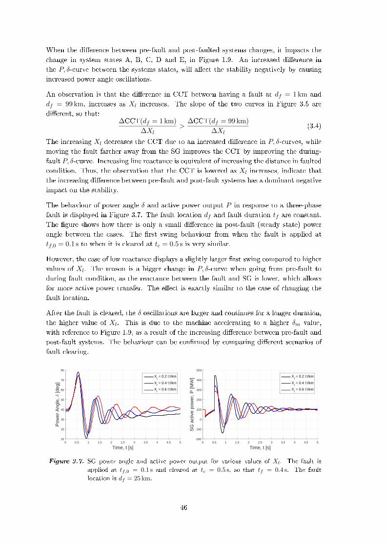
When the dierence between pre-fault and post-faulted systems changes, it impacts the

change in system states A, B, C, D and E, in Figure 1.9. An increased dierence in

the P, δ-curve between the systems states, will aect the stability negatively by causing

increased power angle oscillations.

An observation is that the dierence in CCT between having a fault at df = 1 km and

df = 99 km, increases as Xl increases. The slope of the two curves in Figure 3.5 are

dierent, so that:∆CCT(df = 1 km)

∆Xl>

∆CCT(df = 99 km)

∆Xl(3.4)

The increasing Xl decreases the CCT due to an increased dierence in P, δ-curves, while

moving the fault farther away from the SG improves the CCT by improving the during-

fault P, δ-curve. Increasing line reactance is equivalent of increasing the distance in faulted

condition. Thus, the observation that the CCT is lowered as Xl increases, indicate that

the increasing dierence between pre-fault and post-fault systems has a dominant negative

impact on the stability.

The behaviour of power angle δ and active power output P in response to a three-phase

fault is displayed in Figure 3.7. The fault location df and fault duration tf are constant.

The gure shows how there is only a small dierence in post-fault (steady state) power

angle between the cases. The rst swing behaviour from when the fault is applied at

tf,0 = 0.1 s to when it is cleared at tc = 0.5 s is very similar.

However, the case of low reactance displays a slightly larger rst swing compared to higher

values of Xl. The reason is a bigger change in P, δ-curve when going from pre-fault to

during fault condition, as the reactance between the fault and SG is lower, which allows

for more active power transfer. The eect is exactly similar to the case of changing the

fault location.

After the fault is cleared, the δ oscillations are larger and continues for a longer duration,

the higher value of Xl. This is due to the machine accelerating to a higher δm value,

with reference to Figure 1.9, as a result of the increasing dierence between pre-fault and

post-fault systems. The behaviour can be conrmed by comparing dierent scenarios of

fault clearing.

0 0.5 1 1.5 2 2.5 3 3.5 4 4.5 5

Time, t [s]

10

20

30

40

50

60

70

80

Pow

er A

ngle

, δ [d

eg]

Xl = 0.2 Ω/km

Xl = 0.4 Ω/km

Xl = 0.6 Ω/km

0 0.5 1 1.5 2 2.5 3 3.5 4 4.5 5

Time, t [s]

-200

-100

0

100

200

300

400

500

SG

act

ive

pow

er, P

[MW

] Xl = 0.2 Ω/km

Xl = 0.4 Ω/km

Xl = 0.6 Ω/km

Figure 3.7. SG power angle and active power output for various values of Xl. The fault is

applied at tf,0 = 0.1 s and cleared at tc = 0.5 s, so that tf = 0.4 s. The fault

location is df = 25 km.

46

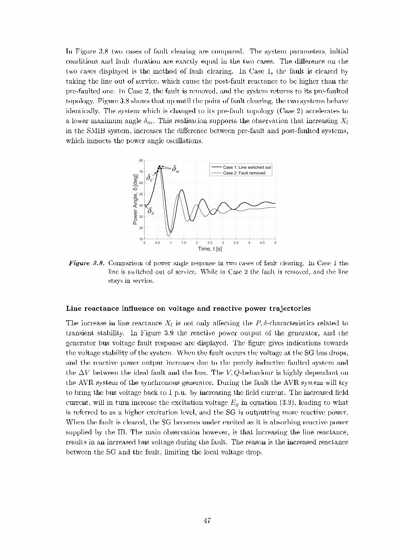
In Figure 3.8 two cases of fault clearing are compared. The system parameters, initial

conditions and fault duration are exactly equal in the two cases. The dierence on the

two cases displayed is the method of fault clearing. In Case 1, the fault is cleared by

taking the line out of service, which cause the post-fault reactance to be higher than the

pre-faulted one. In Case 2, the fault is removed, and the system returns to its pre-faulted

topology. Figure 3.8 shows that up until the point of fault clearing, the two systems behave

identically. The system which is changed to its pre-fault topology (Case 2) accelerates to

a lower maximum angle δm. This realisation supports the observation that increasing Xl

in the SMIB system, increases the dierence between pre-fault and post-faulted systems,

which impacts the power angle oscillations.

0 0.5 1 1.5 2 2.5 3 3.5 4 4.5 5

Time, t [s]

10

20

30

40

50

60

70

80

Pow

er

Angle

,δ

[deg]

Case 1: Line switched out

Case 2: Fault removed

δ0

δC

δm

Figure 3.8. Comparison of power angle response in two cases of fault clearing. In Case 1 the

line is switched out of service. While in Case 2 the fault is removed, and the line

stays in service.

Line reactance inuence on voltage and reactive power trajectories

The increase in line reactance Xl is not only aecting the P, δ-characteristics related to

transient stability. In Figure 3.9 the reactive power output of the generator, and the

generator bus voltage fault response are displayed. The gure gives indications towards

the voltage stability of the system. When the fault occurs the voltage at the SG bus drops,

and the reactive power output increases due to the purely inductive faulted system and

the ∆V between the ideal fault and the bus. The V,Q-behaviour is highly dependant on

the AVR system of the synchronous generator. During the fault the AVR system will try

to bring the bus voltage back to 1 p.u. by increasing the eld current. The increased eld

current, will in turn increase the excitation voltage Eg in equation (3.3), leading to what

is referred to as a higher excitation level, and the SG is outputting more reactive power.

When the fault is cleared, the SG becomes under-excited as it is absorbing reactive power

supplied by the IB. The main observation however, is that increasing the line reactance,

results in an increased bus voltage during the fault. The reason is the increased reactance

between the SG and the fault, limiting the local voltage drop.

47

0 0.1 0.2 0.3 0.4 0.5 0.6 0.7 0.8 0.9 1

Time, t [s]

-300

-200

-100

0

100

200

300

400S

G R

ea

ctive p

ow

er,

Q [

Mva

r] Xl= 0.2 Ω/km

Xl= 0.4 Ω/km

Xl= 0.6 Ω/km

tf,0

tc

0 0.1 0.2 0.3 0.4 0.5 0.6 0.7 0.8 0.9 1

Time, t [s]

0.2

0.4

0.6

0.8

1

SG

bu

s v

olta

ge,

VB, p

.u.

Xl= 0.2 Ω/km

Xl= 0.4 Ω/km

Xl= 0.6 Ω/km

tf,0

tc

Figure 3.9. SG reactive power output and bus voltage for various values of Xl. The fault is

applied at tf,0 = 0.1 s and cleared at tc = 0.5 s, so that tf = 0.4 s. The fault

location is df = 25 km.

3.3.2 Sensitivity of transmission line capacitance

Now capacitance is added to the lossless transmission line. The line reactance is now xed

at a value of Xl = 0.181 Ω/km (L = 0.576 H), which is an example value of underground

cables given by CIGRE in technical brochure B1.30 [37].

Figure 3.10 show the behaviour of CCT on the SMIB system as the transmission line

capacitance is increased. An observation is that there is an insignicant dierence in

CCT between the two cases of fault location (1 km and 99 km), as the capacitance is

increased. The small dierence between the two cases, comes from the dierence in line

reactance between the SG and the faulted location. Transmission line capacitance is a

parallel component, and does not aect the equivalent reactance between the SG and the

fault in the same way as line inductance or resistance does. This behaviour indicates that

the main inuence of capacitance on transient stability, lies in the impact on post-fault

and pre-faulted system power angle, rather than the faulted network topology.

0 50 100 150 200 250

Transmission line capacitance, C [nF/km]

0

0.1

0.2

0.3

0.4

0.5

Crit

ical

cle

arin

g tim

e, C

CT

[s]

df = 1 km

df = 99 km

Figure 3.10. CCT sensitivity of line capacitance C in the SMIB system. The line is lossless,

with Xl = 0.181 Ω/km. Total length of the line, l = 100 km.

In order to exclude that the result is signicantly inuenced by the modelling of the line,

the study is repeated for a SMIB system with a line divided in 5 π-sections of 20 km each,

to be compared with the results of the 100 km π-modelled line.

48

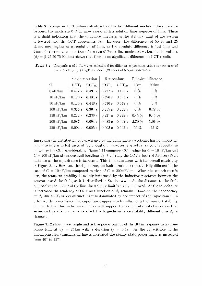
Table 3.1 compares CCT values calculated for the two dierent models. The dierence

between the models is 0 % in most cases, with a solution time step-size of 1 ms. There

is a slight indication that the dierence increases as the stability limit of the system

is lowered and the CCT approaches 0 s. However, the dierences of 50 % and 25

% are meaningless at a resolution of 1 ms, as the absolute dierence is just 1 ms and

2 ms. Furthermore, comparison of the two dierent line models at various fault locations

(df = [1 25 50 75 99] km) shows that there is no signicant dierence in CCT results.

Table 3.1. Comparison of CCT values calculated for dierent capacitance values in two cases of

line modelling: (1) single π-model, (2) series of 5 equal π-sections.

Single π-section 5 π-sections Relative dierence

C CCT1 CCT99 CCT1 CCT99 1 km 99 km

0 nF/km 0.477 s 0.491 s 0.477 s 0.491 s 0 % 0 %

10 nF/km 0.470 s 0.484 s 0.470 s 0.484 s 0 % 0 %

50 nF/km 0.436 s 0.448 s 0.436 s 0.448 s 0 % 0 %

100 nF/km 0.355 s 0.364 s 0.355 s 0.363 s 0 % 0.27 %

150 nF/km 0.222 s 0.230 s 0.221 s 0.229 s 0.45 % 0.43 %

200 nF/km 0.087 s 0.094 s 0.085 s 0.093 s 2.30 % 1.06 %

250 nF/km 0.004 s 0.005 s 0.002 s 0.003 s 50 % 25 %

Improving the distribution of capacitance by including more π-sections, has no important

inuence in the tested cases of fault location. However, the actual value of capacitance

inuences the CCT considerably. Figure 3.11 compares CCT values for C = 10 nF/km and

C = 200 nF/km at various fault locations df . Generally the CCT is lowered for every fault

distance as the capacitance is increased. This is in agreement with the overall sensitivity

in Figure 3.11. However, the dependency on fault location is substantially dierent in the

case of C = 10 nF/km compared to that of C = 200 nF/km. When the capacitance is

low, the transient stability is mainly inuenced by the inductive reactance between the

generator and the fault, as it is described in Section 3.3.1. As the distance to the fault

approaches the middle of the line, the stability limit is highly improved. As the capacitance

is increased the tendency of CCT as a function of df remains. However, the dependency

on df due to Xl is less distinct, as it is dominated by the impact of the capacitance. In

other words, transmission line capacitance appears to be inuencing the transient stability

dierently than line inductance. This result support the aforementioned observation that

series and parallel components aect the large-disturbance stability dierently as df is

changed.

Figure 3.12 show power angle and active power output of the SG in response to a three-

phase fault at df = 25 km with a duration tf = 0.4 s. As the capacitance of the

uncompensated transmission line is increased the steady state power angle is increased

from 40 to 157.

49

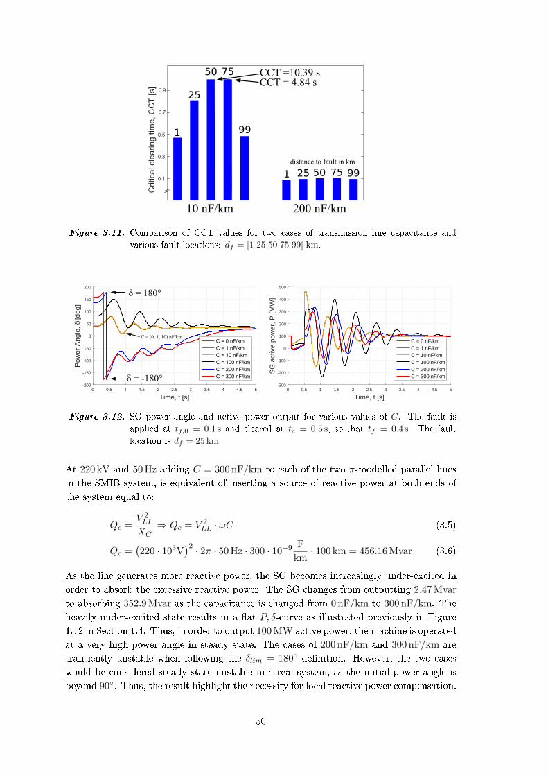
0.1

0.3

0.5

Critica

l cle

arin

g t

ime

, C

CT

[s]

10 nF/km 200 nF/km

1 25 50 75 99

CCT =10.39 s

CCT = 4.84 s

1

25

99

50 75

distance to fault in km

0.7

0.9

Figure 3.11. Comparison of CCT values for two cases of transmission line capacitance and

various fault locations: df = [1 25 50 75 99] km.

0 0.5 1 1.5 2 2.5 3 3.5 4 4.5 5

Time, t [s]

-200

-150

-100

-50

0

50

100

150

200

Po

we

rA

ng

le,δ

[de

g]

C = 0 nF/km

C = 1 nF/km

C = 10 nF/km

C = 100 nF/km

C = 200 nF/km

C = 300 nF/kmδ = -180°

δ = 180°

C = (0, 1, 10) nF/km

0 0.5 1 1.5 2 2.5 3 3.5 4 4.5 5

Time, t [s]

-300

-200

-100

0

100

200

300

400

500

SG

act

ive

pow

er, P

[MW

]

C = 0 nF/kmC = 1 nF/kmC = 10 nF/kmC = 100 nF/kmC = 200 nF/kmC = 300 nF/km

Figure 3.12. SG power angle and active power output for various values of C. The fault is

applied at tf,0 = 0.1 s and cleared at tc = 0.5 s, so that tf = 0.4 s. The fault

location is df = 25 km.

At 220 kV and 50 Hz adding C = 300 nF/km to each of the two π-modelled parallel lines

in the SMIB system, is equivalent of inserting a source of reactive power at both ends of

the system equal to:

Qc =V 2LL

XC⇒ Qc = V 2

LL · ωC (3.5)

Qc =(220 · 103V

)2 · 2π · 50 Hz · 300 · 10−9 F

km· 100 km = 456.16 Mvar (3.6)

As the line generates more reactive power, the SG becomes increasingly under-excited in

order to absorb the excessive reactive power. The SG changes from outputting 2.47 Mvar

to absorbing 352.9 Mvar as the capacitance is changed from 0 nF/km to 300 nF/km. The

heavily under-excited state results in a at P, δ-curve as illustrated previously in Figure

1.12 in Section 1.4. Thus, in order to output 100 MW active power, the machine is operated

at a very high power angle in steady state. The cases of 200 nF/km and 300 nF/km are

transiently unstable when following the δlim = 180 denition. However, the two cases

would be considered steady state unstable in a real system, as the initial power angle is

beyond 90. Thus, the result highlight the necessity for local reactive power compensation.

50

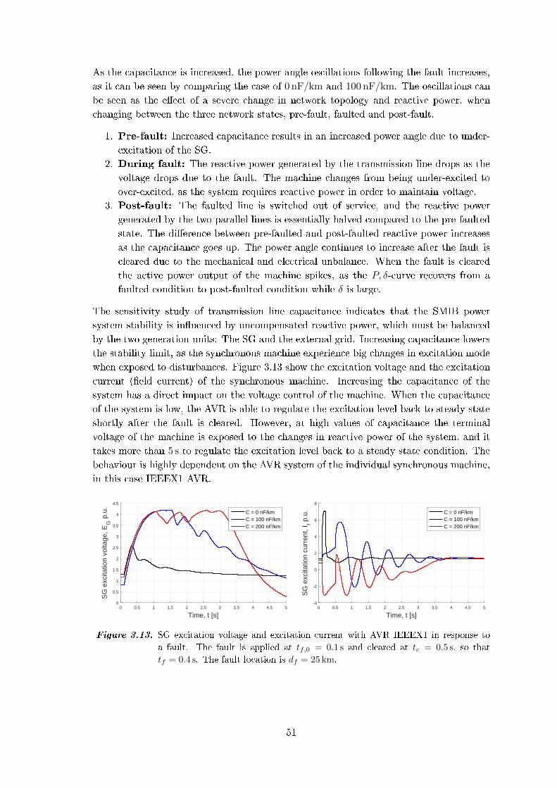
As the capacitance is increased, the power angle oscillations following the fault increases,

as it can be seen by comparing the case of 0 nF/km and 100 nF/km. The oscillations can

be seen as the eect of a severe change in network topology and reactive power, when

changing between the three network states, pre-fault, faulted and post-fault.

1. Pre-fault: Increased capacitance results in an increased power angle due to under-

excitation of the SG.

2. During fault: The reactive power generated by the transmission line drops as the

voltage drops due to the fault. The machine changes from being under-excited to

over-excited, as the system requires reactive power in order to maintain voltage.

3. Post-fault: The faulted line is switched out of service, and the reactive power

generated by the two parallel lines is essentially halved compared to the pre-faulted

state. The dierence between pre-faulted and post-faulted reactive power increases

as the capacitance goes up. The power angle continues to increase after the fault is

cleared due to the mechanical and electrical unbalance. When the fault is cleared

the active power output of the machine spikes, as the P, δ-curve recovers from a

faulted condition to post-faulted condition while δ is large.

The sensitivity study of transmission line capacitance indicates that the SMIB power

system stability is inuenced by uncompensated reactive power, which must be balanced

by the two generation units: The SG and the external grid. Increasing capacitance lowers

the stability limit, as the synchronous machine experience big changes in excitation mode

when exposed to disturbances. Figure 3.13 show the excitation voltage and the excitation

current (eld current) of the synchronous machine. Increasing the capacitance of the

system has a direct impact on the voltage control of the machine. When the capacitance

of the system is low, the AVR is able to regulate the excitation level back to steady state

shortly after the fault is cleared. However, at high values of capacitance the terminal

voltage of the machine is exposed to the changes in reactive power of the system, and it

takes more than 5 s to regulate the excitation level back to a steady state condition. The

behaviour is highly dependent on the AVR system of the individual synchronous machine,

in this case IEEEX1 AVR.

0 0.5 1 1.5 2 2.5 3 3.5 4 4.5 5

Time, t [s]

0

0.5

1

1.5

2

2.5

3

3.5

4

4.5

SG

exc

itatio

n vo

ltage

, EG

p.u

.

C = 0 nF/kmC = 100 nF/kmC = 200 nF/km

0 0.5 1 1.5 2 2.5 3 3.5 4 4.5 5

Time, t [s]

-4

-2

0

2

4

6

8

SG

exc

itatio

n cu

rren

t, I f p

.u. C = 0 nF/km

C = 100 nF/kmC = 200 nF/km

Figure 3.13. SG excitation voltage and excitation current with AVR IEEEX1 in response to

a fault. The fault is applied at tf,0 = 0.1 s and cleared at tc = 0.5 s, so that

tf = 0.4 s. The fault location is df = 25 km.

51

3.3.3 Sensitivity of transmission line AC resistance

Now AC resistance is added to the transmission line. The sensitivity of resistance is

studied in the case of an equivalent OHL. The constant L and C values are based on the

example given in [37]. The values are:

Equivalent OHL: L = 0.858 mH/km, and C = 13.3 nF/km

Figure 3.14 show the CCT sensitivity of increasing transmission line AC resistance.

Typical values of AC resistance are in the area of 0.01 Ω/km to 0.03 Ω/km. In this area

the CCT improves as the resistance is increased. The CCT is more sensitive to changes

in resistance when the fault is located at 99 km compared to when it is located at 1 km.

When the fault is located far from the SG, there is a higher absolute value of resistance

between the SG and the fault, and the faulted topology of the system is aected more by

the increase in resistance. Similar behaviour was observed with line reactance, as both

are series components. The positive inuence of resistance is likely to be caused by a

dampening eect. The dampening is analogous to the case of a RLC-circuit with series

resistance, where the dampening is directly proportional to the resistance of the circuit.

0 0.05 0.1 0.15 0.2 0.25 0.3 0.35 0.4

Transmission line resistance, R [Ω/km]

0.3

0.4

0.5

0.6

0.7

0.8

0.9

Crit

ical

cle

arin

g tim

e, C

CT

[s]

df = 1 km

df = 99 km

Figure 3.14. CCT sensitivity of line AC resistance R in the SMIB system. Two cases of fault

distance df are displayed.

When the resistance is increased above a certain value, the CCT is lowered, and the

stability limit of the SMIB system is decremented. Figure 3.15 show how the power

angle response is changing as the resistance is increased. The fault distance of the cases

displayed is 99 km for comparability to the case displayed in Figure 3.14. As the resistance

is increased, the steady state power angle increases. The reason is that it requires an

increasing angle δ to output 100 MW, due to the resistive part of the impedance seen by

the generator. When the resistance is increased, the maximum angle δm reached after

fault clearing is lowered, and the following oscillations are damped. The red line is the

response at R = 0.2 Ω/km. This is the tested case with best CCT, and it also displays

the most damped power angle oscillations. Increasing the resistance to R = 0.4 Ω/km as

exemplied by the dotted line, displays larger power angle oscillations and lowered CCT.

52

0 0.5 1 1.5 2 2.5 3

Time, t [s]

-20

0

20

40

60

80

100

120

140

SG

pow

er a

ngle

, δ [d

eg] R = 0 Ω/km

R = 0.03 Ω/kmR = 0.2 Ω/kmR = 0.4 Ω/km

Figure 3.15. SG power angle for various values of R. The fault is applied at tf,0 = 0.1 s and

cleared at tc = 0.5 s. The fault location is df = 99 km.

An interesting observation is that in the R = 0.2 Ω/km case, and more distinct in the

case of R = 0.4 Ω/km, the power angle starts by decreasing when the fault occurs, rather

than increasing. The eect is also observed in Figure 3.16, showing that the power output

of the SG increases when the fault occurs, whereas it normally drops. This eect is only

observed as the fault is located near the external grid. A decrease in power angle following

a large disturbance is normally related to the loss of generation or a sudden increase in

load, causing the remaining units to initially decelerate.

0 0.5 1 1.5 2 2.5 3

Time, t [s]

-300

-200

-100

0

100

200

300

400

500

600

SG

act

ive

pow

er, P

[MW

] R = 0 Ω/kmR = 0.03 Ω/kmR = 0.2 Ω/kmR = 0.4 Ω/km

Figure 3.16. SG active power output for various values of R. The fault is applied at tf,0 = 0.1 s

and cleared at tc = 0.5 s. The fault location is df = 99 km.

As the resistance of the transmission line is increased, the XR -ratio approaches 1. The

line reactance is 0.2695 Ω/km, and it is when Rl is close to this value, that the CCT

changes behaviour. This is without accounting for the synchronous reactance, transformer

reactance and the negative shunt reactance. The observation that the decrementing

behaviour in CCT happens around this value could be an indication that the positive eect

of resistance is suppressed as the losses of the system, and the voltage drop associated

with the transmission of active power, goes beyond a certain limit.

53

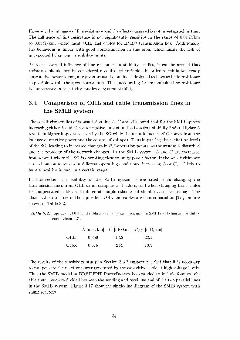
However, the inuence of line resistance and the eects observed is not investigated further.

The inuence of line resistance is not signicantly sensitive in the range of 0.01 Ω/km

to 0.03 Ω/km, where most OHL and cables for HVAC transmission lies. Additionally

the behaviour is linear with good approximation in this area, which limits the risk of

unexpected behaviour in stability limits.

As to the overall inuence of line resistance in stability studies, it can be argued that

resistance should not be considered a controlled variable. In order to minimize steady

state active power losses, any given transmission line is designed to have as little resistance

as possible within the given constraints. Thus, accounting for transmission line resistance

is unnecessary in sensitivity studies of system stability.

3.4 Comparison of OHL and cable transmission lines in

the SMIB system

The sensitivity studies of transmission line L, C and R showed that for the SMIB system

increasing either L and C has a negative impact on the transient stability limits. Higher L

results in higher impedance seen by the SG while the main inuence of C comes from the

balance of reactive power and the control of voltages. Thus impacting the excitation levels

of the SG, leading to increased changes in P, δ-operation points, as the system is disturbed

and the topology of the network changes. In the SMIB system, L and C are increased

from a point where the SG is operating close to unity power factor. If the sensitivities are

carried out on a system in dierent operating conditions, increasing L or C, is likely to

have a positive impact in a certain range.

In this section the stability of the SMIB system is evaluated when changing the

transmission lines from OHL to un-compensated cables, and when changing from cables

to compensated cables with dierent simple schemes of shunt reactor switching. The

electrical parameters of the equivalent OHL and cables are chosen based on [37], and are

shown in Table 3.2.

Table 3.2. Equivalent OHL and cable electrical parameters used in SMIB modelling and stability

comparison [37].

L [mH/km] C [nF/km] RAC [mΩ/km]

OHL 0.858 13.3 23.1

Cable 0.576 234 13.3

The results of the sensitivity study in Section 3.3.2 support the fact that it is necessary

to compensate the reactive power generated by the capacitive cable at high voltage levels.

Thus the SMIB model in DIgSILENT PowerFactory is expanded to include four switch-

able shunt reactors divided between the sending and receiving end of the two parallel lines

in the SMIB system. Figure 3.17 show the single-line diagram of the SMIB system with

shunt reactors.

54

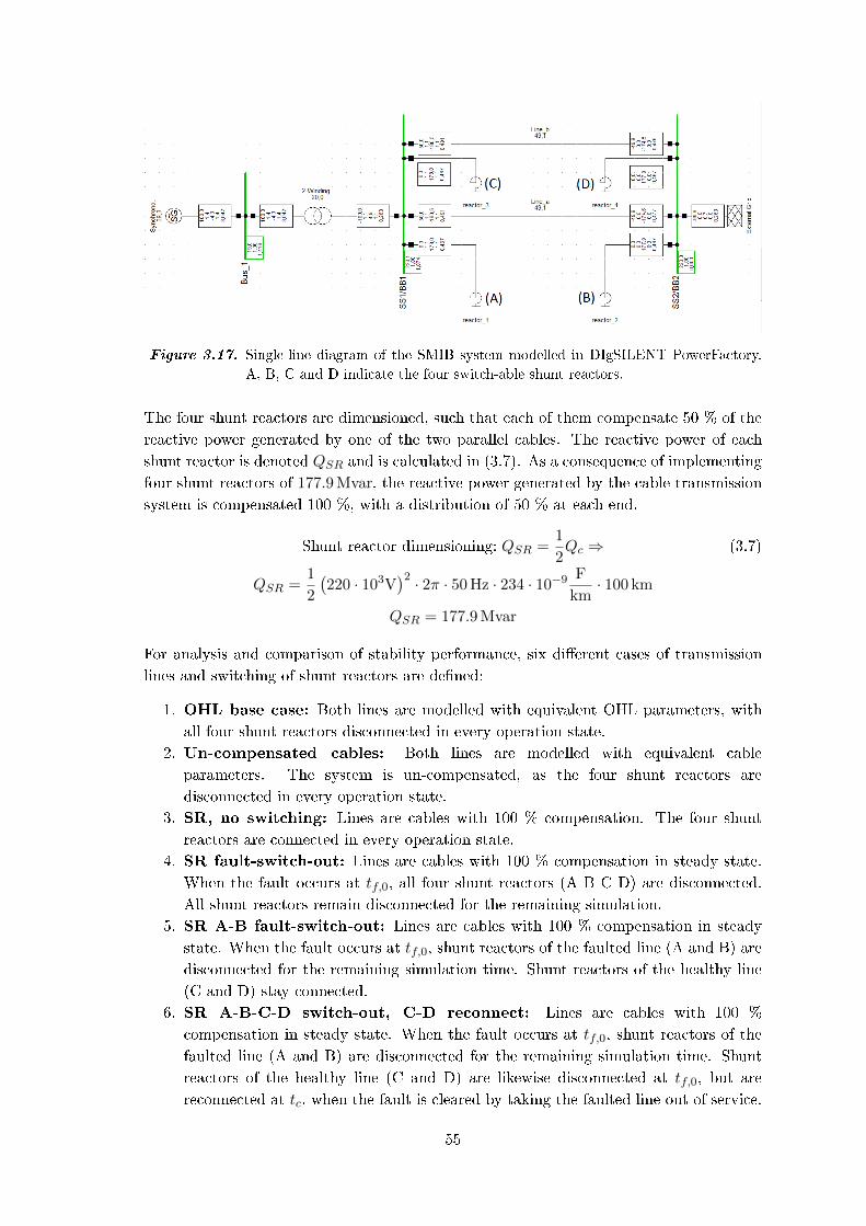
Figure 3.17. Single-line diagram of the SMIB system modelled in DIgSILENT PowerFactory.

A, B, C and D indicate the four switch-able shunt reactors.

The four shunt reactors are dimensioned, such that each of them compensate 50 % of the

reactive power generated by one of the two parallel cables. The reactive power of each

shunt reactor is denoted QSR and is calculated in (3.7). As a consequence of implementing

four shunt reactors of 177.9 Mvar, the reactive power generated by the cable transmission

system is compensated 100 %, with a distribution of 50 % at each end.

Shunt reactor dimensioning: QSR =1

2Qc ⇒ (3.7)

QSR =1

2

(220 · 103V

)2 · 2π · 50 Hz · 234 · 10−9 F

km· 100 km

QSR = 177.9 Mvar

For analysis and comparison of stability performance, six dierent cases of transmission

lines and switching of shunt reactors are dened:

1. OHL base case: Both lines are modelled with equivalent OHL parameters, with

all four shunt reactors disconnected in every operation state.

2. Un-compensated cables: Both lines are modelled with equivalent cable

parameters. The system is un-compensated, as the four shunt reactors are

disconnected in every operation state.

3. SR, no switching: Lines are cables with 100 % compensation. The four shunt

reactors are connected in every operation state.

4. SR fault-switch-out: Lines are cables with 100 % compensation in steady state.

When the fault occurs at tf,0, all four shunt reactors (A B C D) are disconnected.

All shunt reactors remain disconnected for the remaining simulation.

5. SR A-B fault-switch-out: Lines are cables with 100 % compensation in steady

state. When the fault occurs at tf,0, shunt reactors of the faulted line (A and B) are

disconnected for the remaining simulation time. Shunt reactors of the healthy line

(C and D) stay connected.

6. SR A-B-C-D switch-out, C-D reconnect: Lines are cables with 100 %

compensation in steady state. When the fault occurs at tf,0, shunt reactors of the

faulted line (A and B) are disconnected for the remaining simulation time. Shunt

reactors of the healthy line (C and D) are likewise disconnected at tf,0, but are

reconnected at tc, when the fault is cleared by taking the faulted line out of service.

55

The CCT for the dierent cases is calculated by the use of a DPL script in PowerFactory.

For cases 4 and 5, the switching of shunt reactors is independent of the fault duration,

and is easily set up by dening static switch events occurring at the fault incident time

tf,0. However, in case 6, the disconnection of shunt reactors (SR) must be timed with

the removal of the faulted line, at tc. In the DPL script for calculation of CCT tc is

incremented in iterations, till the stability limit δlim is reached. Thus, the switching of

SR C and D must be incremented concurrently. The procedure is visualised by a ow

diagram in Figure 3.18.

Start

End

No

Instabilitytc = CCT

Increase tc and t SR,on

+ 1 ms

tf,0 = 0.1 stc = 0.1 stSR,off = 0.1 stSR,on = 0.1 s

RMS simulation 10 s

δm ≥ δlim

Yes

Set

Figure 3.18. Flow diagram of the CCT method used for Case 6 on the SMIB system.

The CCT values of the case studies are compared in Figure 3.19. The results shown are

for a three-phase fault at 1 km, with removal of the fault by switching the faulted line

out. Placing the fault at 99 km leads to similar results. As expected, when changing

from an OHL system in Case 1 to a un-compensated cable system in Case 2, the CCT

of the system drops to just 17 ms and it is considered unstable, both in steady state and

transiently. As the transmission line is compensated in Case 3, the CCT is signicantly

improved and in this case just above the equivalent OHL case.

Case 4 show the impact of disconnecting all four shunt reactors at the fault incident tf,0.

As the system is faulted, it absorbs an increased amount of reactive power. Shunt reactors

consume reactive power, thus disconnecting shunt reactors in a faulted system condition is

expected to have a positive stability eect, as it should be analogous to injecting reactive

power. However, the results in Figure 3.18 show that disconnecting all shunt reactors at

tf,0 leads to a transiently unstable system.

56

Case 1

Case 2

Case 3

Case 4

Case 5

Case 6

0

0.1

0.2

0.3

0.4

0.5

Critical cle

aring tim

e, C

CT

[s]

461

17

472

0

478 479

Figure 3.19. Simulated CCT values for dierent cases of transmission lines and switching of

shunt compensation. The values above each bar is the actual CCT in ms.

Observing the power angle δ for Case 4 in Figure 3.20 reveals that the SG does not lose

synchronism in the rst-swing. Actually Case 4 display similar rst-swing behaviour as

case 3, 5 and 6, all of which has a high CCT value. In Case 4, following the second power

swing, the angle separation of the SG and the external grid increases. Thus the instability

of Case 4 is likely to be the consequence of not reconnecting the compensation of the

healthy transmission line, leading to an unstable post-faulted system.

In Case 5, the shunt reactors of the faulted line are disconnected, while the shunt reactors of

the healthy parallel line stay in operation. Case 5 display slightly better CCT performance,

than Case 3, where all shunt reactors stay in operation during the fault. This indicates

that lowering the required reactive power during a fault, by disconnecting shunt reactors,

does have an improving eect on transient stability, as long as the healthy lines are still

compensated. Case 4 exemplies the importance of reconnecting shunt reactors. The

small improvement of just 6 ms, between Case 3 and Case 5, indicates that the lowered

reactive power demand due to shunt reactor switching, is not providing sucient leverage

to make a signicant dierence in the case displayed. Although it is important to note

that the fault is located at 1 km, which causes a severe voltage drop at the bus, which can

be seen in Figure 3.21. Case 6 displays a very small improvement in CCT, and is the best

of all the tested cases. Case 6 is similar to the transiently unstable Case 4, as all shunt

reactors are disconnected initially. The important dierence is that the shunt reactors (C

and D) of the healthy line are reconnected, when the fault is cleared by removal of the

faulted line.

57

0 1 2 3 4 5 6 7 8 9 10

Time, t [s]

-200

-150

-100

-50

0

50

100

150

200

SG

pow

er a

ngle

, δ [d

eg]

Case 1Case 2Case 3Case 4Case 5Case 6

Figure 3.20. Comparison of power angle behaviour for Cases 1-6. The fault is located at

df = 1 km and is cleared at tc = 0.4 s, so that tf = 0.3 s.

0 1 2 3 4 5 6 7 8 9 10

Time, t [s]

-500

-400

-300

-200

-100

0

100

200

300

SG

rea

ctiv

e po

wer

, Q [M

var]

Case 1Case 2Case 3Case 4Case 5Case 6

0 1 2 3 4 5 6 7 8 9 10

Time, t [s]

0

0.2

0.4

0.6

0.8

1

1.2

1.4

SG

bus

vol

tage

, V p

.u.

Case 1Case 2Case 3Case 4Case 5Case 6

Figure 3.21. Comparison of SG reactive power and bus voltage for Cases 1-6. The fault is

located at df = 1 km and is cleared at tc = 0.4 s, so that tf = 0.3 s.

58

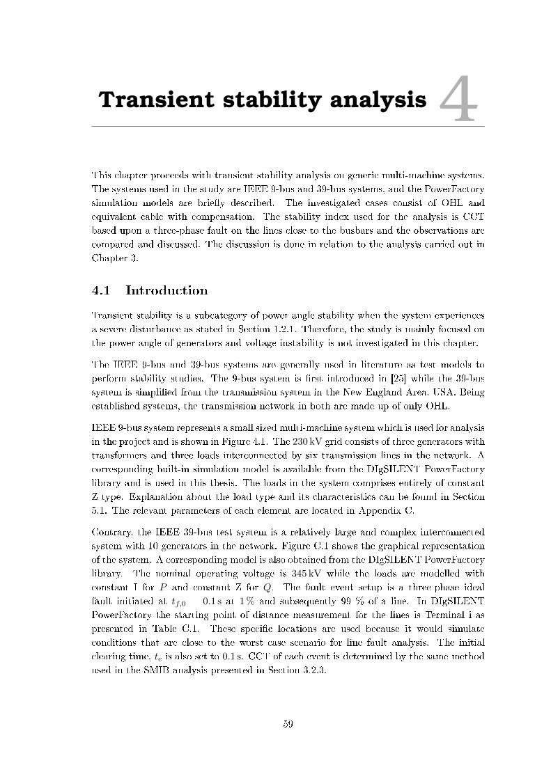
Transient stability analysis 4This chapter proceeds with transient stability analysis on generic multi-machine systems.

The systems used in the study are IEEE 9-bus and 39-bus systems, and the PowerFactory

simulation models are briey described. The investigated cases consist of OHL and

equivalent cable with compensation. The stability index used for the analysis is CCT

based upon a three-phase fault on the lines close to the busbars and the observations are

compared and discussed. The discussion is done in relation to the analysis carried out in

Chapter 3.

4.1 Introduction

Transient stability is a subcategory of power angle stability when the system experiences

a severe disturbance as stated in Section 1.2.1. Therefore, the study is mainly focused on

the power angle of generators and voltage instability is not investigated in this chapter.

The IEEE 9-bus and 39-bus systems are generally used in literature as test models to

perform stability studies. The 9-bus system is rst introduced in [25] while the 39-bus

system is simplied from the transmission system in the New England Area, USA. Being

established systems, the transmission network in both are made up of only OHL.

IEEE 9-bus system represents a small sized multi-machine system which is used for analysis

in the project and is shown in Figure 4.1. The 230 kV grid consists of three generators with

transformers and three loads interconnected by six transmission lines in the network. A

corresponding built-in simulation model is available from the DIgSILENT PowerFactory

library and is used in this thesis. The loads in the system comprises entirely of constant

Z type. Explanation about the load type and its characteristics can be found in Section

5.1. The relevant parameters of each element are located in Appendix C.

Contrary, the IEEE 39-bus test system is a relatively large and complex interconnected

system with 10 generators in the network. Figure C.1 shows the graphical representation

of the system. A corresponding model is also obtained from the DIgSILENT PowerFactory

library. The nominal operating voltage is 345 kV while the loads are modelled with

constant I for P and constant Z for Q. The fault event setup is a three-phase ideal

fault initiated at tf,0 = 0.1 s at 1 % and subsequently 99 % of a line. In DIgSILENT

PowerFactory the starting point of distance measurement for the lines is Terminal i as

presented in Table C.1. These specic locations are used because it would simulate

conditions that are close to the worst case scenario for line fault analysis. The initial

clearing time, tc is also set to 0.1 s. CCT of each event is determined by the same method

used in the SMIB analysis presented in Section 3.2.3.

59

Bus 2

Bus 1

Bus 4

Bus 5 Bus 6

Bus 7

Bus 8

Bus 9

Bus 3

G2 G3

G1

T2

T1

T3 Line 2

Line 3 Line 4

Line 5

Line 1 Line 6 A B

C

Generator

Transformer

Load

Figure 4.1. IEEE 9-bus system single-line diagram.

Since multi-machine systems are investigated, the number of machines detected to be

unstable is also recorded and denoted by ns. The process is repeated for all the lines in

the system. The duration of simulation is chosen to be 11 seconds for each iteration. This

is done to ensure that it would cover both rst-swing instability and interarea instability

as explained in Section 1.2.1. The eects of the interarea oscillations would be more likely

detected in the 39-bus system due to its larger scale. The process ow of determining the

CCT of an event is shown in Figure 4.2.

It is important to note that the CCT method is used to nd the stability limit of a

generator which may not necessarily reect the stability of the system as a whole. In

practice, when a generator loses synchronism it would be disconnected from the grid after

which the system may still be able to maintain stability. Nevertheless the CCT values

found are taken to be the stability indicators of a system in the project.

As mentioned in Section 1.3.2, the stability dening parameter of a multi-machine system

is the angular separation between generators. Consider a simple system with various

identically placed generators of dierent ratings, when the system is subjected to severe

disturbance, there is typically one candidate generator or a group of generators in the

system likely to deviate from the remaining machines which are known as critical machines.

These critical machines are generally the weak machines responsible for any loss of

synchronism. One of the ways to identify such machines is to compare the inertia constant

H or short-circuit power of the machines in the system.

60

Start

End

CCT and ns recorded

No

Check number of out of step machines

Increase tc

Set tf,0 = 0.1 s and tc = 0.1 s

Run RMS simulation for 11 s

At least one machine recording

out of step?

Yes

Figure 4.2. Flow diagram of the CCT method for a single event in multi-machine system.

4.2 IEEE 9-bus transient stability analysis

This section presents the analysis of all the study cases carried out on the IEEE 9-bus

system with regards to transient stability. The default DIgSILENT PowerFactory 9-bus

model is used as the base model for initial sensitivity study. It is followed by increasing

line shunt capacitance, replacing OHL with cable and introducing compensation to the

cable-based system.

4.2.1 IEEE 9-bus transient stability base case

In this case, the fault conditions as described in Section 4.1 are simulated using the base

model. The model is set to operate at default settings and G1 being the generator with

the highest H by referring to Table C.2, is used as the reference machine. The angular

separation of machines are measured relative to the angle of the reference machine. CCT

is determined for each event and tabulated in Table 4.1 in accordance to the line at which

fault is applied. The subscript notation of CCT refers to the location of the fault. For

example, CCT1 stands for the CCT when fault is initiated at 1 % of the line. Terminal i

is included in the table for convenience. Maximum of ns is 2 as unstable detection is not

possible for G1.

61

Table 4.1. CCT recorded for fault applied at each line in base case.

Faulted Line Terminal i CCT1 [ms] ns [-] CCT99 [ms] ns [-]

Line 1 Bus 5 248 1 197 1

Line 2 Bus 7 85 2 172 2

Line 3 Bus 7 117 1 182 1

Line 4 Bus 8 200 1 152 1

Line 5 Bus 9 127 2 228 2

Line 6 Bus 6 275 2 200 2

Based on Table 4.1, the CCT tends to be higher when the fault is located at a distance

farther away from generators. This observation is expected and it veries the principle

explained in Section 1.3.1 because the generator could transfer more active power with

increase in the fault distance away from the sending end, thus having a greater power

curve during fault and improving system stability.

Furthermore, the system has a higher stability margin when the fault happens nearer

to generator G1 as observed by the higher average CCT values recorded when fault is

simulated at Line 1 and Line 6. This is due to G1 having the highest inertia constant,

H as compared to G2 and G3. In any fault event, the generator that is most aected

by the disturbance is the one located nearest to the fault location. Higher H translates

into slower increase in power angle when subjected to disturbance according to (1.2) and

therefore able to sustain fault for a longer period before exceeding the stability limit.

A similar investigation is carried out by changing the reference machine of the base model

to G2 which can be found in Appendix F. In summary, the new case study records the

same CCT values found in the base case.

4.2.2 Increasing line capacitance

This section investigates the inuence of increasing line capacitance of the base model on

the system stability. The sensitivity study can be treated as a transitional analysis to the

equivalent cable-based system. As mentioned in Section 1.1, the main dierence in using

cables is the much higher capacitance value. When using the parameter transformation

ratios as proposed by [37] in the process of replacing the lines with equivalent-cables

which is shown in Section 4.2.3, the model becomes steady-state unstable and power ow

simulation is not possible. Instead the capacitance of each line is multiplied initially by a

small capacitance factor, Fc and increased in steps further because in this way simulations

could be performed until a certain limit of Fc is reached.

Figure 4.3 shows the CCT sensitivity with line capacitance obtained from simulations

performed with fault at 1 % of the rst three lines. A general observation can be made

that the stability performance of the system has a negative tendency with increase in line

capacitance. This is in coherence with the ndings in the SMIB analysis and is explained

in Section 3.3.2.

62

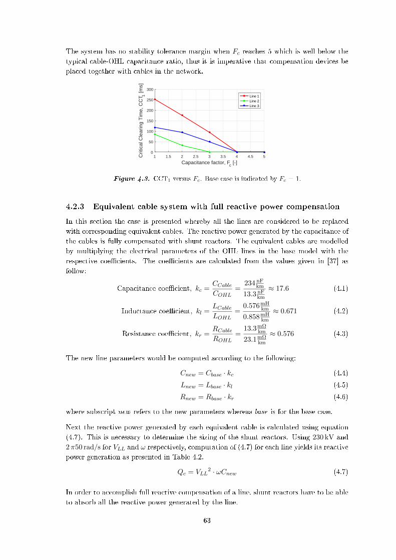
The system has no stability tolerance margin when Fc reaches 5 which is well below the

typical cable-OHL capacitance ratio, thus it is imperative that compensation devices be

placed together with cables in the network.

1 1.5 2 2.5 3 3.5 4 4.5 5

Capacitance factor, Fc [-]

0

50

100

150

200

250

300

Crit

ical

Cle

arin

g T

ime,

CC

T 1 [m

s]

Line 1Line 2Line 3

Figure 4.3. CCT1 versus Fc. Base case is indicated by Fc = 1.

4.2.3 Equivalent cable system with full reactive power compensation

In this section the case is presented whereby all the lines are considered to be replaced

with corresponding equivalent cables. The reactive power generated by the capacitance of

the cables is fully compensated with shunt reactors. The equivalent cables are modelled

by multiplying the electrical parameters of the OHL lines in the base model with the

respective coecients. The coecients are calculated from the values given in [37] as

follow:

Capacitance coecient, kc =CCableCOHL

=234 nF

km

13.3 nFkm

≈ 17.6 (4.1)

Inductance coecient, kl =LCableLOHL

=0.576mH

km

0.858mHkm

≈ 0.671 (4.2)

Resistance coecient, kr =RCableROHL

=13.3mΩ

km

23.1mΩkm

≈ 0.576 (4.3)

The new line parameters would be computed according to the following:

Cnew = Cbase · kc (4.4)

Lnew = Lbase · kl (4.5)

Rnew = Rbase · kr (4.6)

where subscript new refers to the new parameters whereas base is for the base case.

Next the reactive power generated by each equivalent cable is calculated using equation

(4.7). This is necessary to determine the sizing of the shunt reactors. Using 230 kV and

2π50 rad/s for VLL and ω respectively, computation of (4.7) for each line yields its reactive

power generation as presented in Table 4.2.

Qc = VLL2 · ωCnew (4.7)

In order to accomplish full reactive compensation of a line, shunt reactors have to be able

to absorb all the reactive power generated by the line.

63

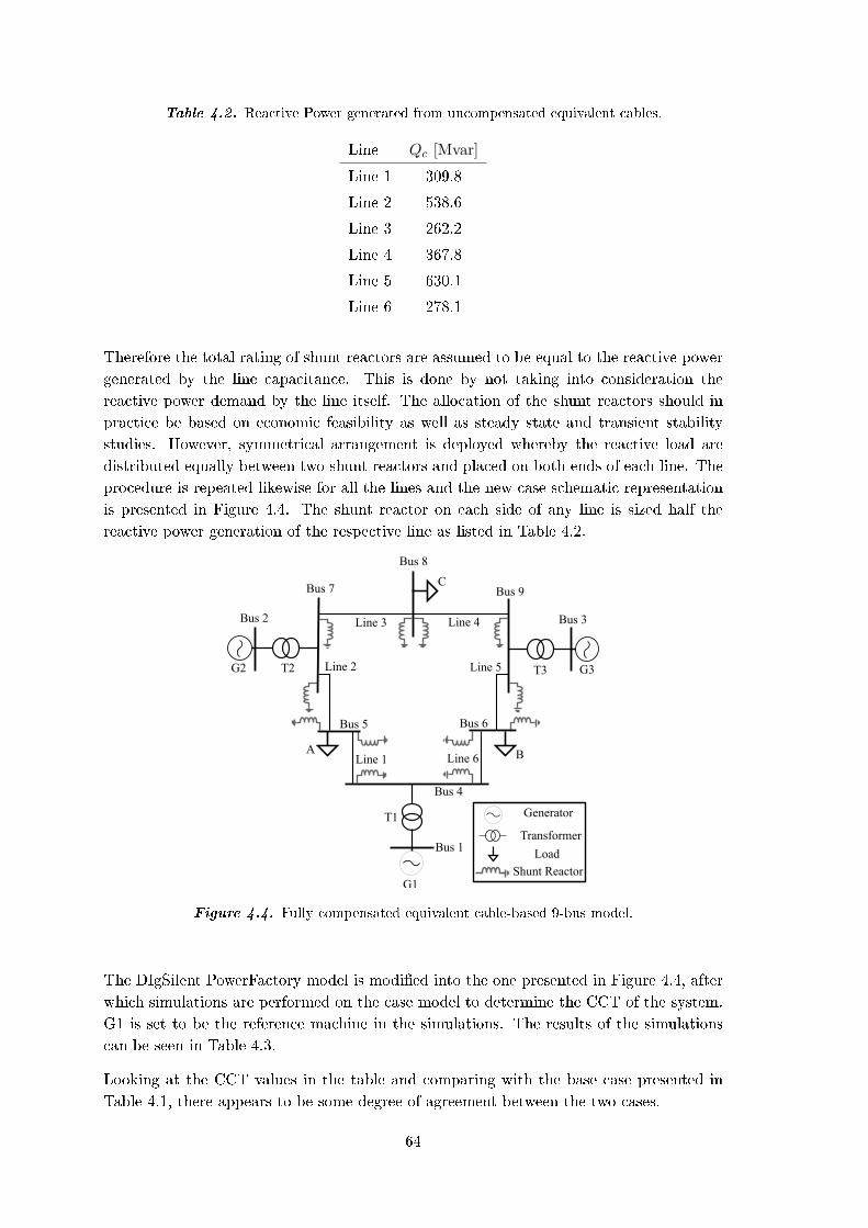
Table 4.2. Reactive Power generated from uncompensated equivalent cables.

Line Qc [Mvar]

Line 1 309.8

Line 2 538.6

Line 3 262.2

Line 4 367.8

Line 5 630.1

Line 6 278.1

Therefore the total rating of shunt reactors are assumed to be equal to the reactive power

generated by the line capacitance. This is done by not taking into consideration the

reactive power demand by the line itself. The allocation of the shunt reactors should in

practice be based on economic feasibility as well as steady state and transient stability

studies. However, symmetrical arrangement is deployed whereby the reactive load are

distributed equally between two shunt reactors and placed on both ends of each line. The

procedure is repeated likewise for all the lines and the new case schematic representation

is presented in Figure 4.4. The shunt reactor on each side of any line is sized half the

reactive power generation of the respective line as listed in Table 4.2.

Bus 2

Bus 1

Bus 4

Bus 5 Bus 6

Bus 7

Bus 8

Bus 9

Bus 3

G2 G3

G1

T2

T1

T3 Line 2

Line 3 Line 4

Line 5

Line 1 Line 6 A B

C

Generator

Transformer

Load

Shunt Reactor

Figure 4.4. Fully compensated equivalent cable-based 9-bus model.

The DIgSilent PowerFactory model is modied into the one presented in Figure 4.4, after

which simulations are performed on the case model to determine the CCT of the system.

G1 is set to be the reference machine in the simulations. The results of the simulations

can be seen in Table 4.3.

Looking at the CCT values in the table and comparing with the base case presented in

Table 4.1, there appears to be some degree of agreement between the two cases.

64

Table 4.3. CCT of the 100 % compensated equivalent cable system.

Faulted Line Terminal i CCT1 [ms] ns [-] CCT99 [ms] ns [-]

Line 1 Bus 5 241 2 190 1

Line 2 Bus 7 49 2 101 2

Line 3 Bus 7 137 1 196 1

Line 4 Bus 8 198 1 162 1

Line 5 Bus 9 101 2 177 2

Line 6 Bus 6 268 2 195 2

Ignoring Line 2 and Line 5, the overall mean deviation in CCT values for all other events

is just approximately 5.78 %.

On the other hand, faults on Line 2 and Line 5 have a relatively large impact in terms

of stability of the cable-based system. When the fault is located at either side of these

two lines, the CCT values decrease by more than 30 % on average in comparison with the

base case indicating a signicant reduction in stability margin.

Figure 4.5 shows the G2 power angle and active power output for a stable event when

a fault is applied at Line 2 for both cases. Although the initial steady-state operating

power angle of G2 is higher in the base case, the compensated system reaches a much

higher peak value during the rst swing period. Therefore rendering the latter being

more susceptible to rst swing instability. This observation can be explained by the large

surplus of reactive power consumption from the shunt reactor connected at Bus 7 after

Line 2 is disconnected. As a result, G2 has to supply for the reactive power decit. As

much more reactive power is needed to be generated by G2, the active power output is

limited by the generator capability. This is applicable for all the lines but the eects

are substantially more noticeable for Line 2 and Line 5 due to the much higher reactive

power generation by the lines as shown in Table 4.2. Referring to Figure 1.9 with a post

fault power curve the generator would need a longer time in order to recover from the

accelerating power caused by the fault and thus recording higher power angles.

Shunt reactor switching

Further investigation is conducted in order to justify the explanation made concerning

shunt reactors being the main cause of the bigger power angle swing seen in Figure 4.5.

For the same stable event, a special case is simulated with the shunt reactor at Bus 7 which

is initially deployed to compensate Line 2, turned o simultaneously with the initiation of

fault at tf,0 = 0.1 s. The power angle and active power curves of generator G2 for this case

are shown in Figure 4.6 together with the case where shunt reactor remains connected. It

can be seen that the power angle of G2 recovers much faster when the shunt reactor is

disconnected as compared to the case that the shunt reactor is connected. This is because

the post fault active power transfer of G2 is much higher in this case, which mean more

decelerating torque on the generator to counter the accelerating eect of the fault.

65

0 0.5 1 1.5 2 2.5 3 3.5 4 4.5 5

Time, t [s]

20

40

60

80

100

120

140G

2 P

ower

Ang

le r

elat

ive

to r

efer

ence

bus

vol

tage

, / [d

eg] Base case

Compensated

0 0.5 1 1.5 2 2.5 3 3.5 4 4.5 5

Time, t [s]

0

20

40

60

80

100

120

140

160

180

200

G2

Act

ive

pow

er, P

[MW

]

Base caseCompensated

Figure 4.5. Comparison of G2 power angle [left] and active power output [right] between base

case and compensated cable case. The fault is applied at tf,0 = 0.1 s and cleared at

tc = 0.13 s, so that tf = 0.03 s. The fault location is at 1 % of Line 2.

This observation indicates that the shunt reactive allocation may have a direct impact

on the lines. There is the possibility that xed symmetrical distribution may not be the

best compensation scheme in certain scenarios. In view of that, it also paves the way to

consider dynamic shunt compensation schemes that are benecial to the system stability.

It could be done in the form of switching in and out of the shunt reactors or using FACTS

devices by which the output could be regulated. Considering that this strategy relates

mainly to the balancing of reactive power and has a direct impact on voltage regulation,

it is covered with more detail in the voltage stability analysis chapter.

0 0.5 1 1.5 2 2.5 3 3.5 4 4.5 5

Time, t [s]

20

40

60

80

100

120

140

G2

Pow

er A

ngle

rel

ativ

e to

ref

eren

ce b

us v

olta

ge, /

[deg

] Shunt reactor connectedShunt reactor disconnected

0 0.5 1 1.5 2 2.5 3 3.5 4 4.5 5

Time, t [s]

0

20

40

60

80

100

120

140

160

180

200

G2

Act

ive

pow

er, P

[MW

]

Shunt reactor connectedShunt reactor disconnected

Figure 4.6. Comparison of G2 power angle [left] and active power output [right] between non

SR switching case and SR switching case. The fault is applied at tf,0 = 0.1 s and

cleared at tc = 0.13 s, so that tf = 0.03 s. The fault location is at 1 % of Line 2.

4.2.4 Variation of reactive power compensation degree

In this section, the degree of reactive power compensation of the equivalent cable system

is varied and the eects on stability are studied. The compensation levels applied from

95% to 115% of the reactive power requirement for each line as listed in Table 4.2.

66

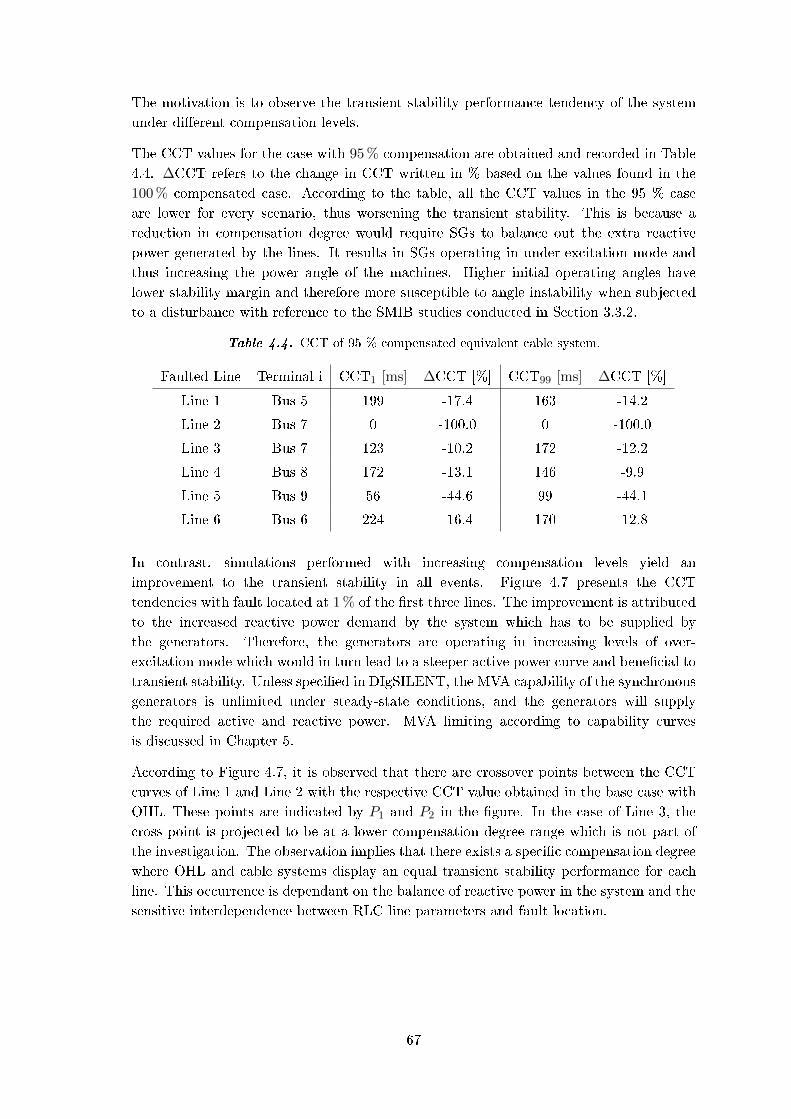
The motivation is to observe the transient stability performance tendency of the system

under dierent compensation levels.

The CCT values for the case with 95 % compensation are obtained and recorded in Table

4.4. ∆CCT refers to the change in CCT written in % based on the values found in the

100 % compensated case. According to the table, all the CCT values in the 95 % case

are lower for every scenario, thus worsening the transient stability. This is because a

reduction in compensation degree would require SGs to balance out the extra reactive

power generated by the lines. It results in SGs operating in under-excitation mode and

thus increasing the power angle of the machines. Higher initial operating angles have

lower stability margin and therefore more susceptible to angle instability when subjected

to a disturbance with reference to the SMIB studies conducted in Section 3.3.2.

Table 4.4. CCT of 95 % compensated equivalent cable system.

Faulted Line Terminal i CCT1 [ms] ∆CCT [%] CCT99 [ms] ∆CCT [%]

Line 1 Bus 5 199 -17.4 163 -14.2

Line 2 Bus 7 0 -100.0 0 -100.0

Line 3 Bus 7 123 -10.2 172 -12.2

Line 4 Bus 8 172 -13.1 146 -9.9

Line 5 Bus 9 56 -44.6 99 -44.1

Line 6 Bus 6 224 -16.4 170 -12.8

In contrast, simulations performed with increasing compensation levels yield an

improvement to the transient stability in all events. Figure 4.7 presents the CCT

tendencies with fault located at 1 % of the rst three lines. The improvement is attributed

to the increased reactive power demand by the system which has to be supplied by

the generators. Therefore, the generators are operating in increasing levels of over-

excitation mode which would in turn lead to a steeper active power curve and benecial to

transient stability. Unless specied in DIgSILENT, the MVA capability of the synchronous

generators is unlimited under steady-state conditions, and the generators will supply

the required active and reactive power. MVA limiting according to capability curves

is discussed in Chapter 5.

According to Figure 4.7, it is observed that there are crossover points between the CCT

curves of Line 1 and Line 2 with the respective CCT value obtained in the base case with

OHL. These points are indicated by P1 and P2 in the gure. In the case of Line 3, the

cross point is projected to be at a lower compensation degree range which is not part of

the investigation. The observation implies that there exists a specic compensation degree

where OHL and cable systems display an equal transient stability performance for each

line. This occurrence is dependant on the balance of reactive power in the system and the

sensitive interdependence between RLC line parameters and fault location.

67

95 100 105 110 115

Compensation degree [%]

0

50

100

150

200

250

300

350

Crit

ical

Cle

arin

g T

ime,

CC

T 1[m

s]

Line 1Line 2Line 3

OHL base case

P1

P2

Figure 4.7. Compensation degree sensitivity comparison. Fault location is at 1% at the line.

4.3 IEEE 39-bus transient stability analysis

This section proceeds with the transient stability analysis on the IEEE 39-bus system. The

system is analysed in a similar manner as in the 9-bus system. The essence of the study

is to determine whether the observations from 9-bus would also hold true for the 39-bus

system, which is more comparable to a real interconnected power system. As a summary,

the 9-bus study presented in Section 4.2 indicates that the fully shunt compensated cable

system is comparable to the uncompensated OHL system in terms of transient stability

performance. Further improvement could be observed by over-compensating, whereas

under-compensation gives rise to an opposite eect.

Taking into account that the 39-bus system is much larger and has a far more complex

nature, much of the investigation would be focused on certain signicant events instead

on all the lines. This is done in order to narrow down the analysis and comparison to the

most important cases.

4.3.1 39-Bus transient stability base case

For the base case, the default DIgSILENT PowerFactory model of the 39-bus system is

used as the base model. Simulations are performed under default settings and G1 is

selected as the reference machine due to its highest inertia constant value. The CCT

values obtained from all the simulated events are shown in Table F.2.

Based on the table, it is evident that the CCT is signicantly higher when the fault is

applied near to G1 which is located at Bus 39. This observation is also consistent with

the ndings in the 9-bus study and is explained in Section 4.2.1. Furthermore there are

some events that have resulted in multiple machines recording unstable detection during

the simulation period. The events with a CCT value lower than 250 ms are selected and

shown in Table 4.5 for ease of reference.

68

Table 4.5. CCT of multiple pole slip events under 250 ms.

Faulted Line Location [%] CCT [ms] ns [-]

2-25 99 115 2

4-5 99 239 2

5-6 1 239 2

5-6 99 227 2

6-7 1 238 2

15-16 99 173 4

16-17 1 136 2

16-21 1 172 2

21-22 1 108 2

21-22 99 92 2

23-24 1 170 2

There is a possibility, especially in a large system, that a certain unstable machine may

have negative inuence on the other machines causing more severe oscillations due to

the interaction between all the machines in the system. As a result, some machines

would go into unstable operation due to the inuence of another machine instead of the

disturbance. Therefore the rst unstable machine is disconnected to avoid any detrimental

impact to the system. Taking that into consideration, an event with multiple pole-slip

record from the list in Table 4.5 is used for further investigation in a separate simulation

case. The case where the fault is applied at 99 % of Line 15-16, is selected due to its highest

number of pole-slip incidents. In this separate case, the rst machine which reaches 180

degrees, is disconnected at CCT. In other words, the critical generator (G4 in this case)

is disconnected at the same instant as the line. The outcome of the simulation is shown

and compared to the original event in Figure 4.8.

0 0.5 1 1.5 2 2.5 3

Time, t [s]

-200

-150

-100

-50

0

50

100

150

200

Pow

er A

ngle

, δ[d

eg]

G2G3G4G5G6G7G8G9G10

180 degrees

0 0.5 1 1.5 2 2.5 3

Time, t [s]

-200

-150

-100

-50

0

50

100

150

200

Pow

er A

ngle

,δ[d

eg]

G2G3G4G5G6G7G8G9G10

180 degrees

Figure 4.8. Power angle of machines for base case [left] and the case where G4 is disconnected

with the line [right]. The fault is applied at tf,0 = 0.1 s and cleared at tc = 0.273 s,

so that tf = 0.173 s. The fault location is at 99 % of Line 15-16.

69

The simulation reveals that all the machines oscillate fairly below the critical angle of 180

degrees and has a higher stability margin in this case. This observation indicates that

the disconnection of an unstable generator is indeed benecial in terms of system-wide

transient stability. The reason being the disruption of the interaction between the critical

machine and other machines, thus any negative impact is reduced. Nonetheless, such a

method, though it performs better in transient stability, may present other problems in

the network e.g. line overloading and voltage drop. This is because when a generator

from one area is disconnected, the local power supply of that area would need to come

from other areas through the transmission lines therefore increasing the loading of certain

lines. Overloading is more likely when the lines are already loaded substantially high

under normal operating scenario which can lead to a chain of events.

Transient instability in large power systems could be manifested in a relatively slower

form as a result of the inter-area oscillations instead of from the rst swing as mentioned

in Section 1.2.1. When a fault is applied and cleared, the disturbance would aect all the

machines behaviour in a corresponding manner with respect to the location of the fault.

Some machines will behave like a cluster and oscillate in near synchronisation. When

multiple clusters are present in the system, the oscillations between the clusters would

cause a certain machine to oscillate beyond its rst swing oscillation.

An example of such a scenario in the 39-bus system is presented in Figure 4.9. It can be

seen in this scenario that a group of machines form a cluster and display similar oscillatory

behaviour. In contrast, G9 is not part of the cluster and the inter-area oscillation eect is

noticeable for this machine where it can be observed from the gure that the rst swing

peak, P1 is lower than the subsequent peak P2. The type of transient instability for this

particular event is not of rst swing nature but rather an outcome of subsequent swings

and therefore would require a much longer simulation time for detection.

0 1 2 3 4 5 6 7 8 9 10 11

Time, t [s]

-40

-20

0

20

40

60

80

100

120

140

160

Pow

er

Angle

, δ[d

eg]

G2

G3

G4

G5

G6

G7

G8

G9

G10

P1

P2

Cluster of machines

Figure 4.9. Power angle fault response of the machines. The fault is applied at tf,0 = 0.1 s and

cleared at tc = 0.1525 s, so that tf = 0.0525 s. The fault location is at 99 % of Line

28-29.

70

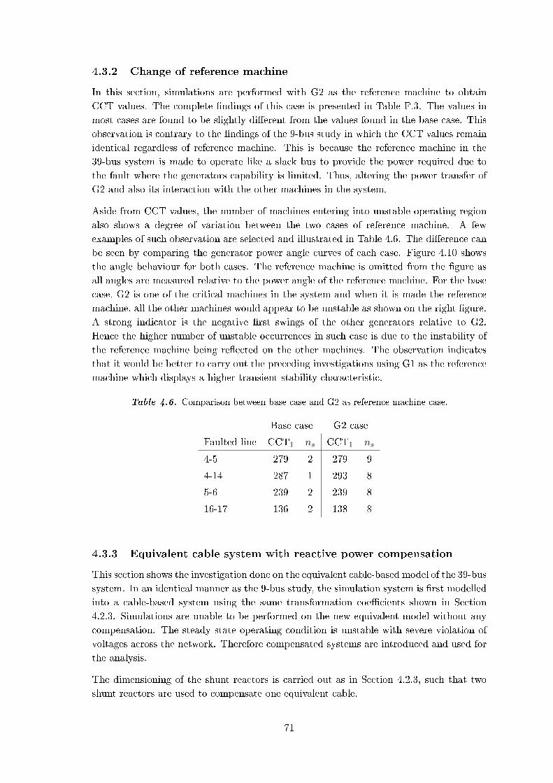
4.3.2 Change of reference machine

In this section, simulations are performed with G2 as the reference machine to obtain

CCT values. The complete ndings of this case is presented in Table F.3. The values in

most cases are found to be slightly dierent from the values found in the base case. This

observation is contrary to the ndings of the 9-bus study in which the CCT values remain

identical regardless of reference machine. This is because the reference machine in the

39-bus system is made to operate like a slack bus to provide the power required due to

the fault where the generators capability is limited. Thus, altering the power transfer of

G2 and also its interaction with the other machines in the system.

Aside from CCT values, the number of machines entering into unstable operating region

also shows a degree of variation between the two cases of reference machine. A few

examples of such observation are selected and illustrated in Table 4.6. The dierence can

be seen by comparing the generator power angle curves of each case. Figure 4.10 shows

the angle behaviour for both cases. The reference machine is omitted from the gure as

all angles are measured relative to the power angle of the reference machine. For the base

case, G2 is one of the critical machines in the system and when it is made the reference

machine, all the other machines would appear to be unstable as shown on the right gure.

A strong indicator is the negative rst swings of the other generators relative to G2.

Hence the higher number of unstable occurrences in such case is due to the instability of

the reference machine being reected on the other machines. The observation indicates

that it would be better to carry out the preceding investigations using G1 as the reference

machine which displays a higher transient stability characteristic.

Table 4.6. Comparison between base case and G2 as reference machine case.

Base case G2 case

Faulted line CCT1 ns CCT1 ns

4-5 279 2 279 9

4-14 287 1 293 8

5-6 239 2 239 8

16-17 136 2 138 8

4.3.3 Equivalent cable system with reactive power compensation

This section shows the investigation done on the equivalent cable-based model of the 39-bus

system. In an identical manner as the 9-bus study, the simulation system is rst modelled

into a cable-based system using the same transformation coecients shown in Section

4.2.3. Simulations are unable to be performed on the new equivalent model without any

compensation. The steady state operating condition is unstable with severe violation of

voltages across the network. Therefore compensated systems are introduced and used for

the analysis.

The dimensioning of the shunt reactors is carried out as in Section 4.2.3, such that two

shunt reactors are used to compensate one equivalent cable.

71

0 0.5 1 1.5 2 2.5 3

Time, t [s]

-200

-150

-100

-50

0

50

100

150

200P

ow

er

Angle

, δ

[deg]

G2

G3

G4

G5

G6

G7

G8

G9

G10

0 0.5 1 1.5 2 2.5 3

Time, t [s]

-200

-150

-100

-50

0

50

100

150

200

Pow

er

Angle

, δ

[deg]

G1

G3

G4

G5

G6

G7

G8

G9

G10

Figure 4.10. Power angle of machines for base case [left] and the case where G2 is reference

machine [right]. The fault is applied at tf,0 = 0.1 s and cleared at tc = 0.379 s, so

that tf = 0.279 s. The fault location is at 1 % of Line 4-5.

The simulated compensation degree variation is from 95 % to 115 %. The variation is

applied to all the lines of the network. The compensation degree is calculated in proportion

to the reactive power generation of each line as listed in Table F.4.

CCT values of the compensated system are recorded and tabulated in Table F.5. Figure

4.11 shows the increasing CCT tendency of ve faulted lines when the compensation degree

is increased. These lines are chosen on the basis of where they are distributed across the

network. The positive inuence of increasing compensation level on the CCT is generally

observed for all lines, except Line 26-29. This observation is coherent with the 9-bus

system which displays a similar tendency. The determining factor is due to the change of

excitation state in the generators which could be referred to in Section 4.2.4.

As for the events involving Line 26-29 (which is a 250 km line), generator G9 will become

unstable regardless of the compensation levels. The problem lies in the disconnection of

the line while keeping the shunt reactors connected. This action is equivalent to losing

1509.20 Mvar of reactive power generation in the area. Though such a scenario is good

for transient stability in most cases by driving the generator into over-excitation mode,

this case is unique as the bus voltages in the area experience a much larger drop because

the huge reactive power demand is not provided locally. Based on the P, δ-characteristic

equation shown in 4.8, an increase in excitation voltage Eg is undermined by a large drop

in the receiving end voltage Vb. As a result, a much atter P, δ-curve would have a negative

impact on the transient stability performance of the generator. This case exemplies the

phenomenon where transient instability is an outcome of voltage instability which displays

the coupling between the phenomena as mentioned in Section 1.2.1.

P =EgVbX

sin(δ) (4.8)

Lastly, the rate of increase in CCT for each line is dierent and it depends on multiple

factors. For instance, the total reactive power generation of the line and its location

relative to the generators.

72

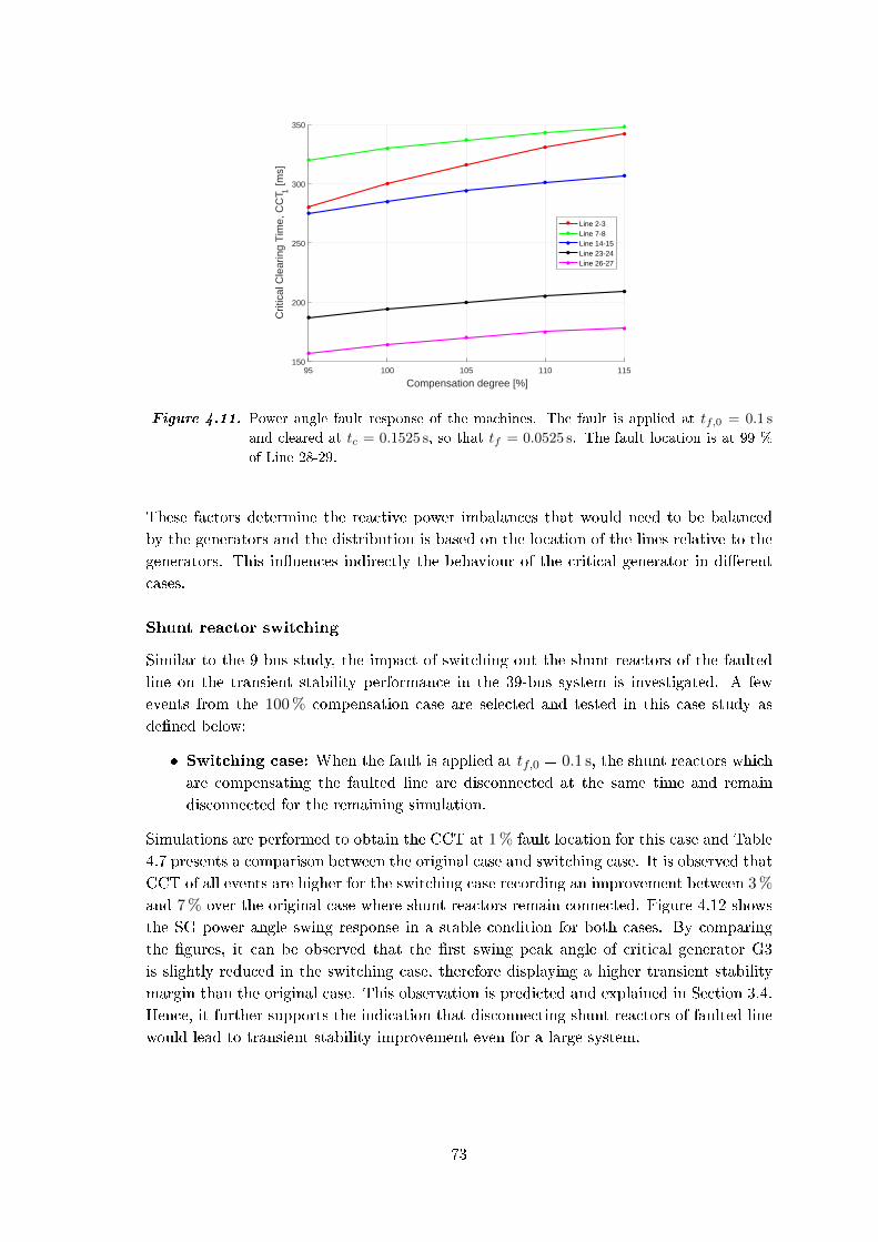
95 100 105 110 115

Compensation degree [%]

150

200

250

300

350

Crit

ical

Cle

arin

g T

ime,

CC

T 1 [m

s]

Line 2-3Line 7-8Line 14-15Line 23-24Line 26-27

Figure 4.11. Power angle fault response of the machines. The fault is applied at tf,0 = 0.1 s

and cleared at tc = 0.1525 s, so that tf = 0.0525 s. The fault location is at 99 %

of Line 28-29.

These factors determine the reactive power imbalances that would need to be balanced

by the generators and the distribution is based on the location of the lines relative to the

generators. This inuences indirectly the behaviour of the critical generator in dierent

cases.

Shunt reactor switching

Similar to the 9-bus study, the impact of switching out the shunt reactors of the faulted

line on the transient stability performance in the 39-bus system is investigated. A few

events from the 100 % compensation case are selected and tested in this case study as

dened below:

Switching case: When the fault is applied at tf,0 = 0.1 s, the shunt reactors which

are compensating the faulted line are disconnected at the same time and remain

disconnected for the remaining simulation.

Simulations are performed to obtain the CCT at 1 % fault location for this case and Table

4.7 presents a comparison between the original case and switching case. It is observed that

CCT of all events are higher for the switching case recording an improvement between 3 %

and 7 % over the original case where shunt reactors remain connected. Figure 4.12 shows

the SG power angle swing response in a stable condition for both cases. By comparing

the gures, it can be observed that the rst swing peak angle of critical generator G3

is slightly reduced in the switching case, therefore displaying a higher transient stability

margin than the original case. This observation is predicted and explained in Section 3.4.

Hence, it further supports the indication that disconnecting shunt reactors of faulted line

would lead to transient stability improvement even for a large system.

73

Table 4.7. CCT comparison between cases with and without switching of shunt reactors.

Faulted Line CCT without switch [ms] CCT with switch [ms] Improvement [%]

3-4 330 342 3.6

2-25 217 232 6.9

9-39 845 897 6.2

14-15 285 308 5.3

22-23 225 240 6.7

0 0.5 1 1.5 2 2.5 3 3.5 4

Time, t [s]

-100

-50

0

50

100

150

200

Pow

er A

ngle

, δ [d

eg]

G2G3G4G5G6G7G8G9G10

0 0.5 1 1.5 2 2.5 3 3.5 4

Time, t [s]

-100

-50

0

50

100

150

200

Pow

er A

ngle

, δ [d

eg]

G2G3G4G5G6G7G8G9G10

Figure 4.12. Power angle of machines for original case [left] and switching case [right]. The

fault is applied at tf,0 = 0.1 s and cleared at tc = 0.380 s, so that tf = 0.280 s. The

fault location is at 1 % of Line 14-15.

4.4 Transient stability summary

This section gives an overview of the transient stability study carried out for the SMIB,

IEEE 9-bus and 39-bus test systems. The large disturbance scenario is created by applying

a three-phase fault on a line and fault clearing by disconnecting the line. The following

are the conclusions of the transient stability analysis in this thesis:

Location of the disturbance is crucial: Transient stability performance is better

when the faults are located farther away from generators. The system stability

margin is higher when the faults are near to strong machines.

Inuence of line parameters: When the generator is initially supplying only

active power across the transmission lines, increasing series inductance and shunt

capacitance of the lines would have a negative impact on CCT. This conclusion is

also applied for system with inductive loads.

The equivalent cable system should be compensated: In SMIB, transient

stability is signicantly improved by compensating the transmission lines consisting

of cables. As for the 9-bus and 39-bus systems, the equivalent cable-based system is

transiently unstable without compensation. In addition, the steady state operation

of each uncompensated system would also be considered unstable.

74

Sizing of shunt reactors matters: Increasing the compensation degree generally

improves transient stability to a certain extent. The reason is the increasing over-

excitation state of the generators. However in reality this positive eect is limited by

the AVR design of generators and the MVA capability. Likewise, undervoltage issues

may also arise that would counter the positive impact of compensation increment.

Eect of dynamic reactor switching: By disconnecting the shunt reactors of

the faulted line during and after fault, leads to improvement in CCT.

Impact of machine controls: AVR and excitation system in the generator model

are important factors inuencing the dynamic change of states - pre, during and

post disturbance. Cables and compensation are strongly inuenced by the control

model.

75

Large-disturbance voltagestability analysis: IEEE

9-bus system 5This chapter describes the study of large-disturbance voltage stability on the IEEE 9-bus

system. Similarly to the presented transient stability analysis in Chapter 4, the OHL base

case is compared to cases of equivalent cable transmission lines. Dierent strategies for

reactive power compensation is analysed, with focus on switching in response to large-

disturbances and dynamic compensation. The analysis also includes the comparison of

dierent load models and their impact on the results in voltage stability studies.

Load modelling: Comparison of dierent load models in voltage stability studies.

Q,V-characteristics: Producing and analysing Q,V -curves to locate system weak-

points.

Voltage trajectories: Analysis of voltage trajectories following large-disturbances.

Reactive power compensation: Analysis of dierent reactive power compensa-

tion strategies for improvement of voltage stability.

5.1 Load modelling in voltage stability analysis

In stability studies load modelling plays an essential role, as it aects the dynamic response

of the system. Just like it is typical practice in power system analysis, loads are represented

involving simplications and by summation of the characteristics of several dierent loads,

such as induction motors, heaters, compressors, lights and so forth. Where induction

motors are estimated to account for 60-70 % of the total load [2]. A widely used load

modelling method, which is described in both [2] and the DIgSILENT PowerFactory

version 15.1.6 documentation [38], is the polynomial model:

P = P0

(p1

(v

v0

)ep,1+ p2

(v

v0

)ep,2+ p3

(v

v0

)ep,3)(5.1)

Q = Q0

(q1

(v

v0

)eq,1+ q2

(v

v0

)eq,2+ q3

(v

v0

)eq,3)(5.2)

Expressions (5.1) and (5.2) model the load bus P,Q as a nonlinear function of the bus

voltage v. Both expressions can be expanded to include dependency on the electrical

frequency. However, frequency variations are not accounted for in the study of voltage

stability in this thesis. The term v0 is the initial bus voltage under normal operation

conditions, where P = P0 and Q = Q0.

77

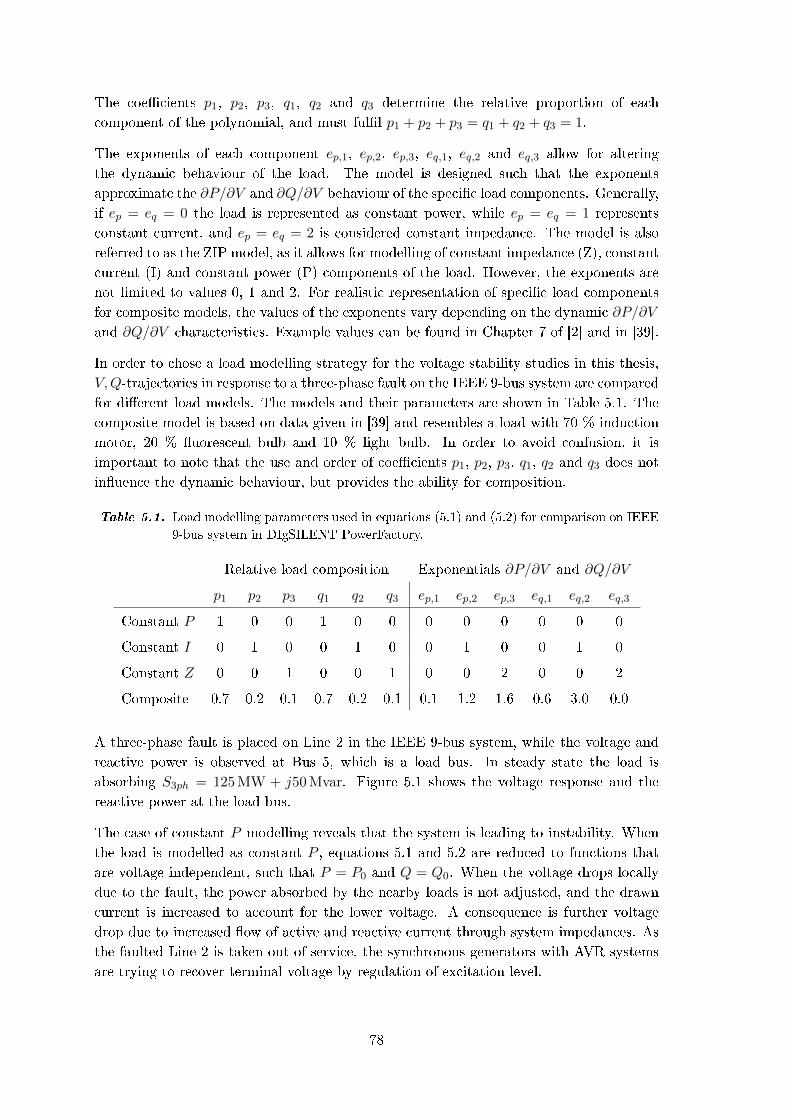
The coecients p1, p2, p3, q1, q2 and q3 determine the relative proportion of each

component of the polynomial, and must full p1 + p2 + p3 = q1 + q2 + q3 = 1.

The exponents of each component ep,1, ep,2, ep,3, eq,1, eq,2 and eq,3 allow for altering

the dynamic behaviour of the load. The model is designed such that the exponents

approximate the ∂P/∂V and ∂Q/∂V behaviour of the specic load components. Generally,

if ep = eq = 0 the load is represented as constant power, while ep = eq = 1 represents

constant current, and ep = eq = 2 is considered constant impedance. The model is also

referred to as the ZIP model, as it allows for modelling of constant impedance (Z), constant

current (I) and constant power (P) components of the load. However, the exponents are

not limited to values 0, 1 and 2. For realistic representation of specic load components

for composite models, the values of the exponents vary depending on the dynamic ∂P/∂V

and ∂Q/∂V characteristics. Example values can be found in Chapter 7 of [2] and in [39].

In order to chose a load modelling strategy for the voltage stability studies in this thesis,

V,Q-trajectories in response to a three-phase fault on the IEEE 9-bus system are compared

for dierent load models. The models and their parameters are shown in Table 5.1. The

composite model is based on data given in [39] and resembles a load with 70 % induction

motor, 20 % uorescent bulb and 10 % light bulb. In order to avoid confusion, it is

important to note that the use and order of coecients p1, p2, p3, q1, q2 and q3 does not

inuence the dynamic behaviour, but provides the ability for composition.

Table 5.1. Load modelling parameters used in equations (5.1) and (5.2) for comparison on IEEE

9-bus system in DIgSILENT PowerFactory.

Relative load composition Exponentials ∂P/∂V and ∂Q/∂V

p1 p2 p3 q1 q2 q3 ep,1 ep,2 ep,3 eq,1 eq,2 eq,3

Constant P 1 0 0 1 0 0 0 0 0 0 0 0

Constant I 0 1 0 0 1 0 0 1 0 0 1 0

Constant Z 0 0 1 0 0 1 0 0 2 0 0 2

Composite 0.7 0.2 0.1 0.7 0.2 0.1 0.1 1.2 1.6 0.6 3.0 0.0

A three-phase fault is placed on Line 2 in the IEEE 9-bus system, while the voltage and

reactive power is observed at Bus 5, which is a load bus. In steady state the load is

absorbing S3ph = 125 MW + j50 Mvar. Figure 5.1 shows the voltage response and the

reactive power at the load bus.

The case of constant P modelling reveals that the system is leading to instability. When

the load is modelled as constant P , equations 5.1 and 5.2 are reduced to functions that

are voltage independent, such that P = P0 and Q = Q0. When the voltage drops locally

due to the fault, the power absorbed by the nearby loads is not adjusted, and the drawn

current is increased to account for the lower voltage. A consequence is further voltage

drop due to increased ow of active and reactive current through system impedances. As

the faulted Line 2 is taken out of service, the synchronous generators with AVR systems

are trying to recover terminal voltage by regulation of excitation level.

78

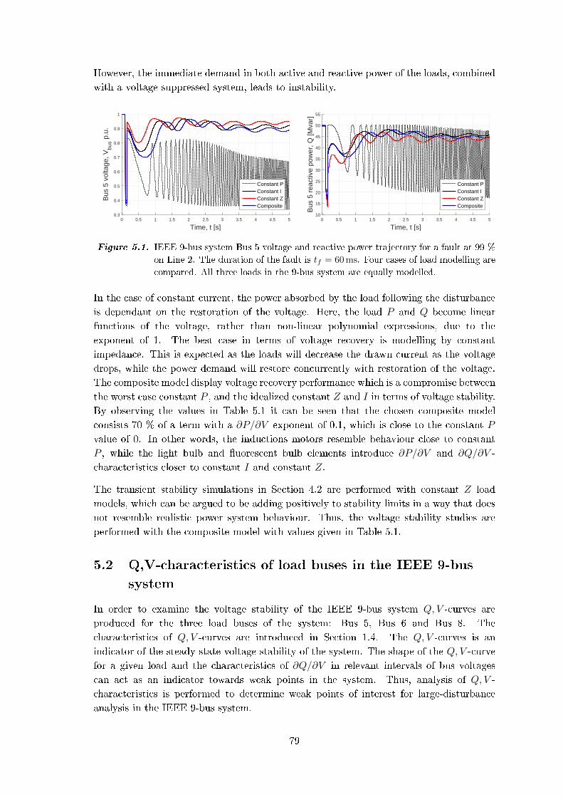
However, the immediate demand in both active and reactive power of the loads, combined

with a voltage suppressed system, leads to instability.

0 0.5 1 1.5 2 2.5 3 3.5 4 4.5 5

Time, t [s]

0.3

0.4

0.5

0.6

0.7

0.8

0.9

1

Bus

5 v

olta

ge, V

bus p

.u.

Constant PConstant IConstant ZComposite

0 0.5 1 1.5 2 2.5 3 3.5 4 4.5 5

Time, t [s]

10

15

20

25

30

35

40

45

50

55

Bus

5 r

eact

ive

pow

er, Q

[Mva

r]

Constant PConstant IConstant ZComposite

Figure 5.1. IEEE 9-bus system Bus 5 voltage and reactive power trajectory for a fault at 99 %

on Line 2. The duration of the fault is tf = 60 ms. Four cases of load modelling are

compared. All three loads in the 9-bus system are equally modelled.

In the case of constant current, the power absorbed by the load following the disturbance

is dependant on the restoration of the voltage. Here, the load P and Q become linear

functions of the voltage, rather than non-linear polynomial expressions, due to the

exponent of 1. The best case in terms of voltage recovery is modelling by constant

impedance. This is expected as the loads will decrease the drawn current as the voltage

drops, while the power demand will restore concurrently with restoration of the voltage.

The composite model display voltage recovery performance which is a compromise between

the worst case constant P , and the idealized constant Z and I in terms of voltage stability.

By observing the values in Table 5.1 it can be seen that the chosen composite model

consists 70 % of a term with a ∂P/∂V exponent of 0.1, which is close to the constant P

value of 0. In other words, the inductions motors resemble behaviour close to constant

P , while the light bulb and uorescent bulb elements introduce ∂P/∂V and ∂Q/∂V -

characteristics closer to constant I and constant Z.

The transient stability simulations in Section 4.2 are performed with constant Z load

models, which can be argued to be adding positively to stability limits in a way that does

not resemble realistic power system behaviour. Thus, the voltage stability studies are

performed with the composite model with values given in Table 5.1.

5.2 Q,V-characteristics of load buses in the IEEE 9-bus

system

In order to examine the voltage stability of the IEEE 9-bus system Q,V -curves are

produced for the three load buses of the system: Bus 5, Bus 6 and Bus 8. The

characteristics of Q,V -curves are introduced in Section 1.4. The Q,V -curves is an

indicator of the steady state voltage stability of the system. The shape of the Q,V -curve

for a given load and the characteristics of ∂Q/∂V in relevant intervals of bus voltages

can act as an indicator towards weak points in the system. Thus, analysis of Q,V -

characteristics is performed to determine weak points of interest for large-disturbance

analysis in the IEEE 9-bus system.

79

The Q,V -curves are produced in DIgSILENT PowerFactory by inserting a variable source

of reactive power at the bus of interest. The injected reactive power Qi is incremented,

rst as being capacitive (positive injection) and followed by inductive (negative injection).

The power ow is solved for every value of Qi, while the resulting change in bus voltage

VB is observed.

Figure 5.2 shows the Q,V -characteristic of Bus 8. It is important to note the dierence

between the rated value of shunt reactive power and the actual injected reactive power

Qi. Due to the non-linear relation of reactive power with the voltage, Qi = V 2/X, the

dierence between rated and actual values increases as the voltage diers further from

the rated 1 p.u. value. When the bus voltage is in the range of 0.85 to 1.15 p.u. the

slope dQ/dV is approximately constant, and the dierence in rated and actual values is

small. Evidently, the two curves intersect at Qi = 0. The dierence between the actual

injected reactive power Qi and the net ow of reactive power is due to the presence of

the composite modelled load at Bus 8. The load is inductive and consumes 35 Mvar when

the voltage is 1 p.u. However, The reactive power characteristics of the load is dependent

on the ∂Q/∂V exponents of the model according to Table 5.1. The dierence between

the two curves increase as the voltage moves further away from 1 p.u. as the voltage

dependency of the load scales according to the modelled exponents.

0.4 0.6 0.8 1 1.2 1.4

Bus 8 voltage in p.u.

-3000

-2500

-2000

-1500

-1000

-500

0

500

1000

Bu

s 8

Re

active

po

we

r, Q

[M

va

r]

Rated shunt capacity

Actual injected reactive power Qi

Net flow of reactive power

∂Q∂V

= 0

Qrated = Qactual

Figure 5.2. Q,V-characteristic of Bus 8 in the IEEE 9-bus system. The loading of the system

is in accordance to the composite model of Table 5.1.

Based on the Q,V -characteristic, Bus 8 proves to have a high voltage stability margin

in steady state, as it requires around 1000 Mvar of rated inductive shunt reactance to

bring the voltage down to the critical voltage level, where ∂Q∂V = 0. For Bus 5 and Bus 6,

the required rated inductive shunt reactance is likewise around 1100 Mvar to 1200 Mvar.

In other words, even though Bus 8 is considered the weakest bus based on the Q,V -

characteristics, it displays a large stability margin, and does not dier signicantly from

Bus 5 and Bus 6.

Figure 5.3 show the Q,V -characteristic of the three load buses in the IEEE 9-bus system.

Bus 5 and Bus 6 display very similar behaviour with equal critical voltages around 0.51

p.u.

80

Bus 5 and Bus 6 are both connected to SG1, which is the machine in the 9-bus system

with the highest MVA rating and acts as slack bus for the power ow solution. Bus 8 has

a slightly higher critical voltage of 0.53 p.u. Thus, Bus 8 is chosen as point of interest

in the 9-bus system for analysis of large-disturbance voltage stability. However, for the

tested load level all three system nodes display satisfactory steady state voltage stability

margin as the critical voltages are far from typical under-voltage limits in steady state.

0.4 0.6 0.8 1 1.2 1.4

Bus voltage in p.u.

-400

-200

0

200

400

600

800

Inje

cte

d r

ea

ctive

po

we

r, Q

i[M

va

r]

Bus 5

Bus 6

Bus 8

0.51 p.u. 0.53 p.u.

Figure 5.3. Q,V-characteristic of the three load buses in the IEEE 9-bus system produced in

DIgSILENT PowerFactory. The loading of the system is in accordance to the

composite model of Table 5.1.

5.3 Voltage stability of Bus 8 in the IEEE 9-bus system

The voltage stability is analysed for the IEEE 9-bus system with use of the discussed

composite load model and by using Bus 8 as point of interest in the system. The stability

is assessed in the case of an OHL based system, and compared to cases of equivalent

cable systems with various degrees of reactive power compensation. The modelling of the

equivalent cable cases and sizing and location of shunt reactors is done according to the

method described in Section 4.2.3.

Figure 5.4 compares the V, P -characteristics of Bus 8 in the OHL base case with three cases

of cable based system. The cables of the system are 100 % compensated. The two cases

referred to as 75 % and 125 % compensation, only involves under and over-compensation

of Line 3 and Line 4 connecting Bus 8 in the ring network. The compensation degree

of the remaining lines remains 100 %. The power factor at Bus 8 is held constant at

0.9438 lagging, which is the nominal value. Thus, as the active power loading is increased,

the reactive power loading is increased coherently. Attention should be directed towards

the dierence between the solid and the dotted lines in Figure 5.4. Due to the voltage

dependency of load P and Q according to the composite load modelling by (5.1) and (5.2),

there is an increasing dierence in V, P -characteristics between composite model and the

nominal P0, Q0 values as the voltage is decreased by the increased loading. It is important

to be aware of this double response, as changes in nominal P0 and Q0 aects the voltage,

which aects the actual P and Q loading.

81

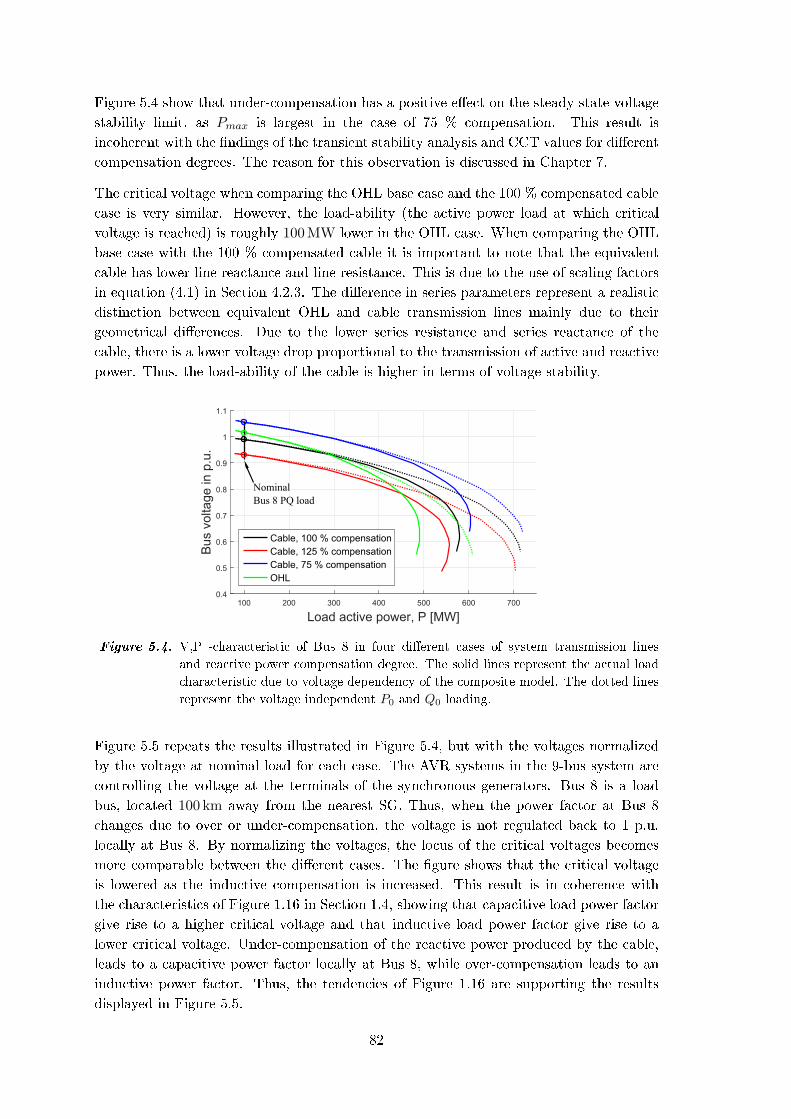
Figure 5.4 show that under-compensation has a positive eect on the steady state voltage

stability limit, as Pmax is largest in the case of 75 % compensation. This result is

incoherent with the ndings of the transient stability analysis and CCT values for dierent

compensation degrees. The reason for this observation is discussed in Chapter 7.

The critical voltage when comparing the OHL base case and the 100 % compensated cable

case is very similar. However, the load-ability (the active power load at which critical

voltage is reached) is roughly 100 MW lower in the OHL case. When comparing the OHL

base case with the 100 % compensated cable it is important to note that the equivalent

cable has lower line reactance and line resistance. This is due to the use of scaling factors

in equation (4.1) in Section 4.2.3. The dierence in series parameters represent a realistic

distinction between equivalent OHL and cable transmission lines mainly due to their

geometrical dierences. Due to the lower series resistance and series reactance of the

cable, there is a lower voltage drop proportional to the transmission of active and reactive

power. Thus, the load-ability of the cable is higher in terms of voltage stability.

100 200 300 400 500 600 700

Load active power, P [MW]

0.4

0.5

0.6

0.7

0.8

0.9

1

1.1

Bu

s v

olta

ge

in

p.u

.

Cable, 100 % compensation

Cable, 125 % compensation

Cable, 75 % compensation

OHL

Nominal

Bus 8 PQ load

Figure 5.4. V,P -characteristic of Bus 8 in four dierent cases of system transmission lines

and reactive power compensation degree. The solid lines represent the actual load

characteristic due to voltage dependency of the composite model. The dotted lines

represent the voltage independent P0 and Q0 loading.

Figure 5.5 repeats the results illustrated in Figure 5.4, but with the voltages normalized

by the voltage at nominal load for each case. The AVR systems in the 9-bus system are

controlling the voltage at the terminals of the synchronous generators. Bus 8 is a load

bus, located 100 km away from the nearest SG. Thus, when the power factor at Bus 8

changes due to over or under-compensation, the voltage is not regulated back to 1 p.u.

locally at Bus 8. By normalizing the voltages, the locus of the critical voltages becomes

more comparable between the dierent cases. The gure shows that the critical voltage

is lowered as the inductive compensation is increased. This result is in coherence with

the characteristics of Figure 1.16 in Section 1.4, showing that capacitive load power factor

give rise to a higher critical voltage and that inductive load power factor give rise to a

lower critical voltage. Under-compensation of the reactive power produced by the cable,

leads to a capacitive power factor locally at Bus 8, while over-compensation leads to an

inductive power factor. Thus, the tendencies of Figure 1.16 are supporting the results

displayed in Figure 5.5.

82

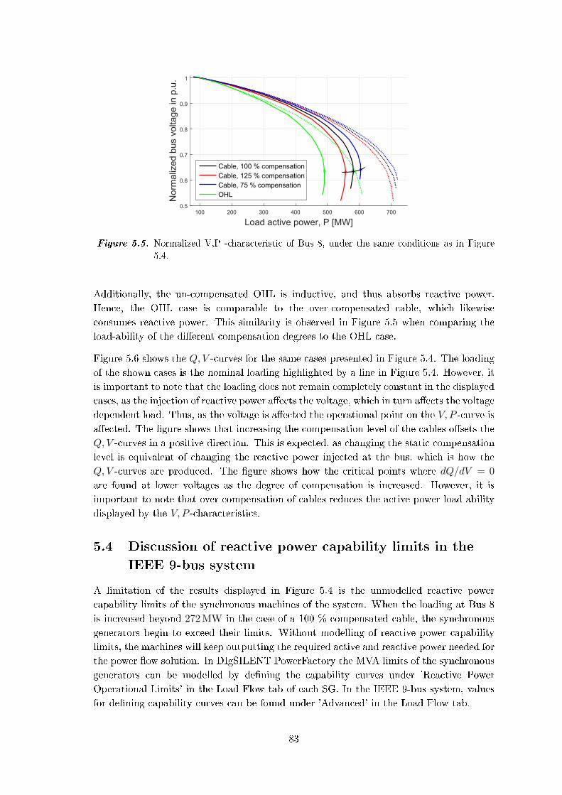
100 200 300 400 500 600 700

Load active power, P [MW]

0.5

0.6

0.7

0.8

0.9

1

No

rma

lize

d b

us v

olta

ge

in

p.u

.Cable, 100 % compensation

Cable, 125 % compensation

Cable, 75 % compensation

OHL

Figure 5.5. Normalized V,P -characteristic of Bus 8, under the same conditions as in Figure

5.4.

Additionally, the un-compensated OHL is inductive, and thus absorbs reactive power.

Hence, the OHL case is comparable to the over-compensated cable, which likewise

consumes reactive power. This similarity is observed in Figure 5.5 when comparing the

load-ability of the dierent compensation degrees to the OHL case.

Figure 5.6 shows the Q,V -curves for the same cases presented in Figure 5.4. The loading

of the shown cases is the nominal loading highlighted by a line in Figure 5.4. However, it

is important to note that the loading does not remain completely constant in the displayed

cases, as the injection of reactive power aects the voltage, which in turn aects the voltage

dependent load. Thus, as the voltage is aected the operational point on the V, P -curve is

aected. The gure shows that increasing the compensation level of the cables osets the

Q,V -curves in a positive direction. This is expected, as changing the static compensation

level is equivalent of changing the reactive power injected at the bus, which is how the

Q,V -curves are produced. The gure shows how the critical points where dQ/dV = 0

are found at lower voltages as the degree of compensation is increased. However, it is

important to note that over-compensation of cables reduces the active power load-ability

displayed by the V, P -characteristics.

5.4 Discussion of reactive power capability limits in the

IEEE 9-bus system

A limitation of the results displayed in Figure 5.4 is the unmodelled reactive power

capability limits of the synchronous machines of the system. When the loading at Bus 8

is increased beyond 272 MW in the case of a 100 % compensated cable, the synchronous

generators begin to exceed their limits. Without modelling of reactive power capability

limits, the machines will keep outputting the required active and reactive power needed for

the power ow solution. In DIgSILENT PowerFactory the MVA limits of the synchronous

generators can be modelled by dening the capability curves under 'Reactive Power

Operational Limits' in the Load Flow tab of each SG. In the IEEE 9-bus system, values

for dening capability curves can be found under 'Advanced' in the Load Flow tab.

83

0.4 0.6 0.8 1 1.2 1.4

Bus voltage in p.u.

-600

-400

-200

0

200

400

600

800

Inje

cted

rea

ctiv

e po

wer

, Qi [M

var]

Cable, 100 % compensationCable, 125 % compensationCable, 75 % compensationOHL

Figure 5.6. Q,V-characteristic of Bus 8 in four dierent cases of system transmission lines and

reactive power compensation degree. The system loading of the displayed case is

the nominal loading of the system.

The capability curves dened using these values are displayed in Figure 5.7.

Two capability curves for SG1 are displayed. The dotted line represent the capability

curve of SG1 directly using the values in PowerFactory, whereas the solid line represent a

capability curve modied to match the shape of SG2 and SG3. Due to the unconventional

shape of SG1, DIgSILENT support was contacted in order to clarify the origin of the

values given in the 'Advanced' tab:

"The capability curves are normally provided by the manufacturer. However, the drawing

(i.e. capability curves based on the values in the advanced tab) is the theoretical

representation using the machine parameters. The parameter xd for this machine (i.e.

SG1) is small compared to the other machines, that's the reason for such a drawing." -

Karla Mendez, DIgSILENT support, 04.05.2016

-250 -200 -150 -100 -50 0 50 100 150 200

Under-excitation

SG1

SG2

SG3

Over-excitationQo [Mvar]

Po [MW]

50

100

150

200

Figure 5.7. Reactive power capability curves of the synchronous machines in the IEEE 9-bus

system in PowerFactory. The capability curves for SG2 and SG3 are directly dened

from the values given in PowerFactory. The capability curve of SG1 is modied

(solid line). The unmodied line is shown as dotted.

84

Thus, the capability curves in Figure 5.7 do not represent real synchronous machines,

but are estimates based on the machine parameters. Nevertheless, the characteristics are

applied in order to exemplify the inuence of limits to reactive power capabilities.

Figure 5.8 shows the V, P -characteristic of Bus 8 in the IEEE 9-bus system in the 100 %

compensated cable case. Three cases are displayed, 1) without capability limits (similar

to the characteristics in Figure 5.4, 2) with capability limits on all three generators,

and 3) with the un-adjusted SG1 capability curve. Figure 5.8 shows that when reactive

power capability limits are modelled, there exists a load level where all three synchronous

generators are operated at their limits.

100 150 200 250 300 350 400 450 500 550 600

Load active power, P [MW]

0.55

0.6

0.65

0.7

0.75

0.8

0.85

0.9

0.95

1

Bus v

oltage in p

.u.

No capability limits

Applied SG1, SG2 and SG3 capability limits

Un-adjusted SG1 capability

Power flow unable

to converge

Figure 5.8. Comparison of V, P -characteristics of Bus 8 in the IEEE 9-bus system.

Increasing the loading at Bus 8 beyond this point, result in the inability to solve the

power ow in PowerFactory. SG1 is acting as slackbus for the power ow solution, thus

attempting to balance active and reactive power beyond the capability of SG1 leads to

failure. It is important to note that this is a general limitation of the power ow solution.

The expected response in a real power system would be an increasing drop in voltage

and frequency as the load level exceeds the generation limits, and not an abrupt system

failure.

The apparent power output So of each synchronous machine, at the loading limit leading

to power ow failure on the next increment, is shown in Figure 5.9. The loading of each

machine at this operating point is:

SG1: So,lim = 231.9 MW + j91.9 Mvar (5.3)

SG2: So,lim = 163.0 MW + j97.0 Mvar (5.4)

SG3: So,lim = 85.0 MW + j81.8 Mvar (5.5)

By observing Figure 5.8 it can be seen that there is a signicant dierence in the loading

leading to power ow failure, dependent on the capability curve of SG1. If the over-

excitation level of SG1 is very low, it changes the power ow of the system even at low

loading. The result is a lower voltage in the area of Bus 8, as SG2 and SG3 must supply the

majority of reactive power for the entire system. The inability of SG1 to supply sucient

reactive power with this capability characteristic, leads to power ow failure at a lower

load level.

85

-150 -100 -50 0 50 100 150 200

Qo [Mvar]

Po [MW]

50

100

150

200

SG1 SSG1,lim

SSG2,lim

SSG3,lim

SG2

SG3

Figure 5.9. Reactive power capability curves of the SGs in the IEEE 9-bus system. The

operating points indicate the apparent power output of the machines when the

loading at Bus 8 is increased to Sload,C = 272 MW + j95.2 Mvar.

As stated, the un-modied reactive power capability curve of SG1 is expected to be

unrealistic. However, the case illustrates the consequence of limited reactive power

capabilities of synchronous machines with respect to system voltages.

Now, recalling the comparison of normalized V, P -characteristics for OHL networks and

cable based networks in Figure 5.5. It can be argued that the dierence in critical voltages

and load-ability of the dierent transmission line topologies in the 9-bus system is trivial.

The MVA limits of the synchronous machines are exceeded before the loading is increased

to a level where any signicant dierence is observed. Thus, if the 9-bus system represents

a real power system, the V, P -characteristics would be dominated by the reactive power

capability of the generators.

However, the V, P -characteristics still provide useful indications towards the voltage

stability margins of the system, as basis for further analysis.

5.5 Voltage trajectory analysis of Bus 8 in the IEEE 9-bus

system

For the initial study of large-disturbance voltage stability, the voltage trajectory method

presented in Section 1.6.4 of the introduction is conducted. The goal is to quantify and

compare the voltage recovery ability for the OHL base case and cable based systems with

dierent reactive power compensation.

For the purpose of making example, Figure 5.10 show the voltage trajectory of Bus 8 for

a three-phase fault on Line 4 in the 9-bus system. The fault is cleared after 60 ms by

removal of Line 4. Two cases are displayed, the voltage trajectory of an OHL transmission

system and the equivalent 100 % SR compensated cable case. The under-voltage limit is

dened according to Figure 1.29 in Section 1.6.4 of the introduction.

86

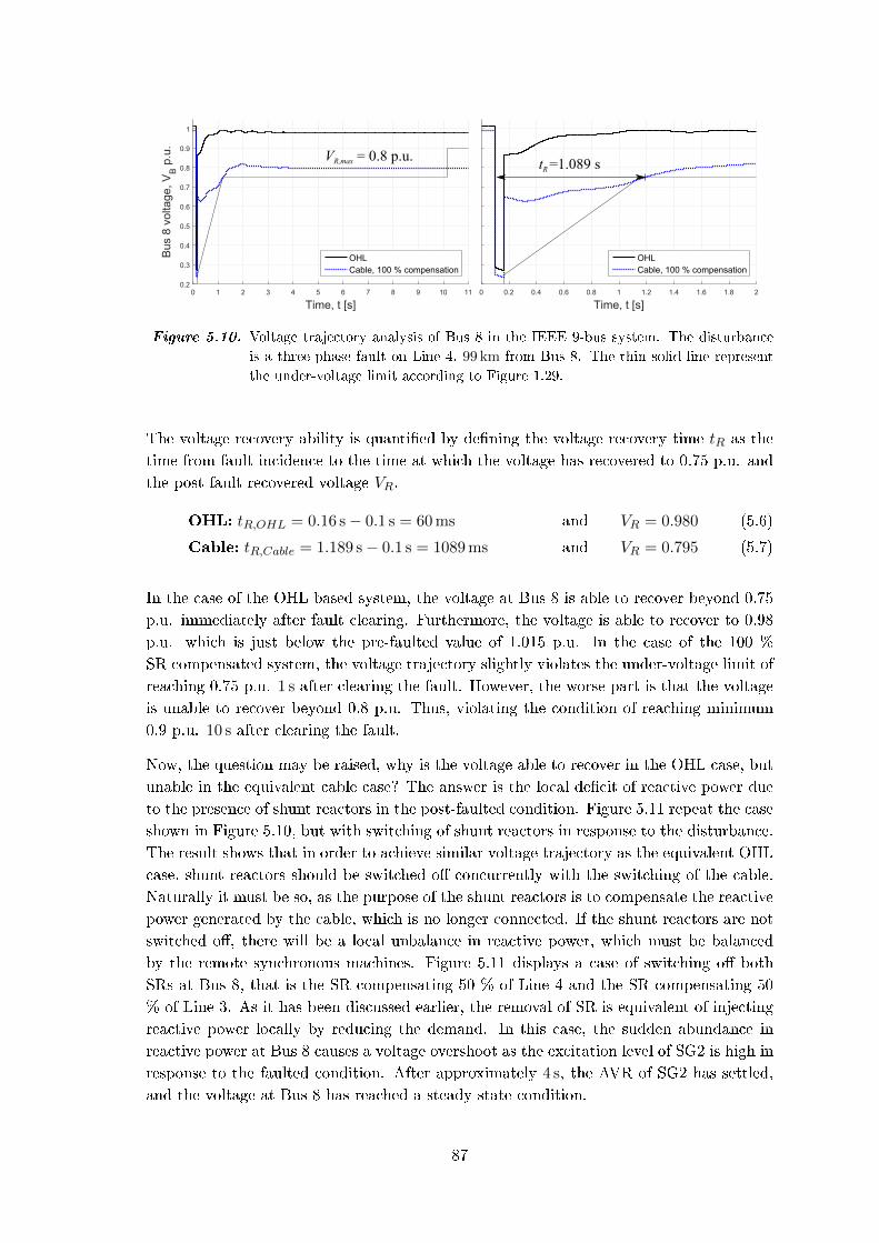
0 1 2 3 4 5 6 7 8 9 10 11

Time, t [s]

0.2

0.3

0.4

0.5

0.6

0.7

0.8

0.9

1

Bus 8

voltage, V

Bp.u

.

OHL

Cable, 100 % compensation

0 0.2 0.4 0.6 0.8 1 1.2 1.4 1.6 1.8 2

Time, t [s]

OHL

Cable, 100 % compensation

tR =1.089 sVR,max = 0.8 p.u.

Figure 5.10. Voltage trajectory analysis of Bus 8 in the IEEE 9-bus system. The disturbance

is a three-phase fault on Line 4, 99 km from Bus 8. The thin solid line represent

the under-voltage limit according to Figure 1.29.

The voltage recovery ability is quantied by dening the voltage recovery time tR as the

time from fault incidence to the time at which the voltage has recovered to 0.75 p.u. and

the post fault recovered voltage VR.

OHL: tR,OHL = 0.16 s− 0.1 s = 60 ms and VR = 0.980 (5.6)

Cable: tR,Cable = 1.189 s− 0.1 s = 1089 ms and VR = 0.795 (5.7)

In the case of the OHL based system, the voltage at Bus 8 is able to recover beyond 0.75

p.u. immediately after fault clearing. Furthermore, the voltage is able to recover to 0.98

p.u. which is just below the pre-faulted value of 1.015 p.u. In the case of the 100 %

SR compensated system, the voltage trajectory slightly violates the under-voltage limit of

reaching 0.75 p.u. 1 s after clearing the fault. However, the worse part is that the voltage

is unable to recover beyond 0.8 p.u. Thus, violating the condition of reaching minimum

0.9 p.u. 10 s after clearing the fault.

Now, the question may be raised, why is the voltage able to recover in the OHL case, but

unable in the equivalent cable case? The answer is the local decit of reactive power due

to the presence of shunt reactors in the post-faulted condition. Figure 5.11 repeat the case

shown in Figure 5.10, but with switching of shunt reactors in response to the disturbance.

The result shows that in order to achieve similar voltage trajectory as the equivalent OHL

case, shunt reactors should be switched o concurrently with the switching of the cable.

Naturally it must be so, as the purpose of the shunt reactors is to compensate the reactive

power generated by the cable, which is no longer connected. If the shunt reactors are not

switched o, there will be a local unbalance in reactive power, which must be balanced

by the remote synchronous machines. Figure 5.11 displays a case of switching o both

SRs at Bus 8, that is the SR compensating 50 % of Line 4 and the SR compensating 50

% of Line 3. As it has been discussed earlier, the removal of SR is equivalent of injecting

reactive power locally by reducing the demand. In this case, the sudden abundance in

reactive power at Bus 8 causes a voltage overshoot as the excitation level of SG2 is high in

response to the faulted condition. After approximately 4 s, the AVR of SG2 has settled,

and the voltage at Bus 8 has reached a steady state condition.

87

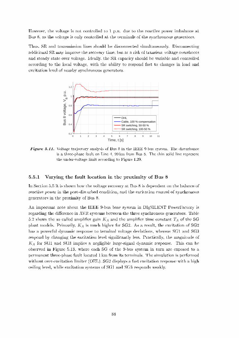
However, the voltage is not controlled to 1 p.u. due to the reactive power imbalance at

Bus 8, as the voltage is only controlled at the terminals of the synchronous generators.

Thus, SR and transmission lines should be disconnected simultaneously. Disconnecting

additional SR may improve the recovery time, but at a risk of transient voltage overshoots

and steady state over voltage. Ideally, the SR capacity should be variable and controlled

according to the local voltage, with the ability to respond fast to changes in load and

excitation level of nearby synchronous generators.

0 1 2 3 4 5 6 7 8 9 10 11

Time, t [s]

0.2

0.4

0.6

0.8

1

1.2

Bus

8 v

olta

ge, V

B p

.u.

OHLCable, 100 % compensationSR switching, 50-50 %SR switching, 100-50 %

Figure 5.11. Voltage trajectory analysis of Bus 8 in the IEEE 9-bus system. The disturbance

is a three-phase fault on Line 4, 99 km from Bus 8. The thin solid line represent

the under-voltage limit according to Figure 1.29.

5.5.1 Varying the fault location in the proximity of Bus 8

In Section 5.5 it is shown how the voltage recovery at Bus 8 is dependent on the balance of

reactive power in the post-disturbed condition, and the excitation control of synchronous

generators in the proximity of Bus 8.

An important note about the IEEE 9-bus base system in DIgSILENT PowerFactory is

regarding the dierence in AVR systems between the three synchronous generators. Table

5.2 shows the so called amplier gain KA and the amplier time constant TA of the SG

plant models. Primarily, KA is much higher for SG2. As a result, the excitation of SG2

has a powerful dynamic response to terminal voltage deviations, whereas SG1 and SG3

respond by changing the excitation level signicantly less. Practically, the magnitude of

KA for SG1 and SG3 implies a negligible large-signal dynamic response. This can be

observed in Figure 5.13, where each SG of the 9-bus system in turn are exposed to a

permanent three-phase fault located 1 km from its terminals. The simulation is performed

without over-excitation limiter (OEL). SG2 displays a fast excitation response with a high

ceiling level, while excitation systems of SG1 and SG3 responds weakly.

88

Table 5.2. Selected AVR system constants of the SGs in the IEEE 9-bus system in DIgSILENT

PowerFactory. KA is the voltage controller gain, while TA is the time constant.

KA [-] TA [s]

SG1 0.001 0.2

SG2 400 0.05

SG3 0.001 0.2

0 2 4 6 8 10 12 14 16 18 20

Time, t [s]

1

2

3

4

5

6

7

8

9

10

Exc

itatio

n vo

ltage

, EG

in p

.u. SG1

SG2SG3

0 5 10 15 20

1.4

1.6

1.8

2

Zoom

Figure 5.12. Excitation system response of the synchronous generators in the IEEE 9-bus

system in response to a permanent three-phase fault located 1 km from the SG

terminals in each respective case.

The dierence in AVR system between the synchronous generators in the 9-bus system

implies another asymmetry in the network, which inuences the voltage stability limits.

Basically, it can be argued that with the base AVR systems, SG2 is the only unit in the

9-bus system with dynamic reactive power and voltage control capabilities. Thus, any

large-signal voltage disturbances would need to rely on the capability of SG2.

Based on this observation, it is relevant to discuss the strength of the network buses, as

it was presented in Section 5.2. Based on the Q,V -curves presented in Figure 5.3, Bus 8

is argued to be the weakest bus in the network. However, the method of producing Q,V

and V, P -curves is a steady state method of assessing voltage stability. Thus, assessing the

strength of the nodes based on the Q,V -curve does not reveal limitations in the dynamic

response of nearby synchronous generators.

Now, it can be argued that Bus 6 is the dynamically weakest bus of the 9-bus system,

as it is the most distant bus relative to SG2, and recalling that SG2 is the only dynamic

regulator of reactive power in the network. However, the important conclusion of this

discussion is not which bus of the 9-bus system is the weakest. Rather, the importance is

how the strength at a given node is aected by the topological change of the network in

post-faulted condition.

Figure 5.13 show how the voltage trajectory at Bus 8 is dependent on the post-faulted

topology relative to SG2. Line 3 is the direct connection between Bus 8 and SG2. Thus,

when Line 3 is faulted and switched out of operation, the voltage trajectory is unable to

satisfy the post-disturbance under-voltage limit.

89

Due to the post-faulted topology of the network in this case, the only dynamic reactive

power controller (i.e. SG2) is distanced far from Bus 8. In contrary, when Line 4 is faulted,

which connects Bus 8 and SG3, the voltage trajectory at Bus 8 is improved as the direct

connection between Bus 8 and SG2 is maintained. Thus, any bus which is separated from

SG2 will be weakened with respect to voltage stability.

The voltage is unable to recover to 1. p.u. due to the post-faulted topology of the network

and the fact that SGs regulate the terminal voltage and not the distant voltage at Bus 8.

0 1 2 3 4 5 6 7 8 9 10 11

Time, t [s]

0

0.2

0.4

0.6

0.8

1

Bu

s 8

vo

lta

ge

, V

Bp

.u.

Line 3, df= 1 km

Line 3, df= 99 km

Line 4, df= 1 km

Line 4, df= 99 km

0 0.2 0.4 0.6 0.8 1 1.2

Time, t [s]

Line 3, df= 1 km

Line 3, df= 99 km

Line 4, df= 1 km

Line 4, df= 99 km

Line 4

Line 3

0

0.1

0.2

0.3

0.4

0.5

0.6

0.7

0.8

Figure 5.13. Voltage trajectory analysis of Bus 8 in the IEEE 9-bus system. Four cases of

line faults are displayed with distances measured from Bus 8. The thin solid line

represent the under-voltage limit according to Figure 1.29.

The AVR systems in the 9-bus system in PowerFactory could simply be changed to

have similar performance. However, as the purpose is to compare the performance of

OHL and cable networks, the dierence in AVR system is just something to be aware of

when assessing the dynamic voltage performance. The discussion highlights that voltage

stability is a local phenomena, which is highly dependent on the reactive power capabilities

of units in the proximity of the area. Based on which the discussion of switching of shunt

reactors in response to large-disturbances becomes relevant.

5.6 Forcing voltage instability in the IEEE 9-bus system

It is desired to investigate if switching of shunt reactors in the cable based HVAC

transmission network provides the ability to stabilize a potential voltage collapse. In

order to realize this study in the IEEE 9-bus system, the system must be disturbed in

such a way that one or more bus voltage does not satisfy the under-voltage limits within

the specied time restrictions.

Such an event can be obtained when applying a series of disturbances to the network.

Initially Line 3 is exposed to a three-phase fault located at 1 % line distance from Bus 8.

After 60 ms the fault is cleared by taking Line 3 out of service, while the shunt reactors

of the line are switched-o correspondingly. However, faulting the system and removal of

a transmission line and SRs does not lead to low system voltage alone, as it is discussed

in Section 5.5. Thus, a load event is introduced where the P,Q loading of Bus 8 start

increasing with a ramp increment in which the load is increased proportionally by 70 %.

90

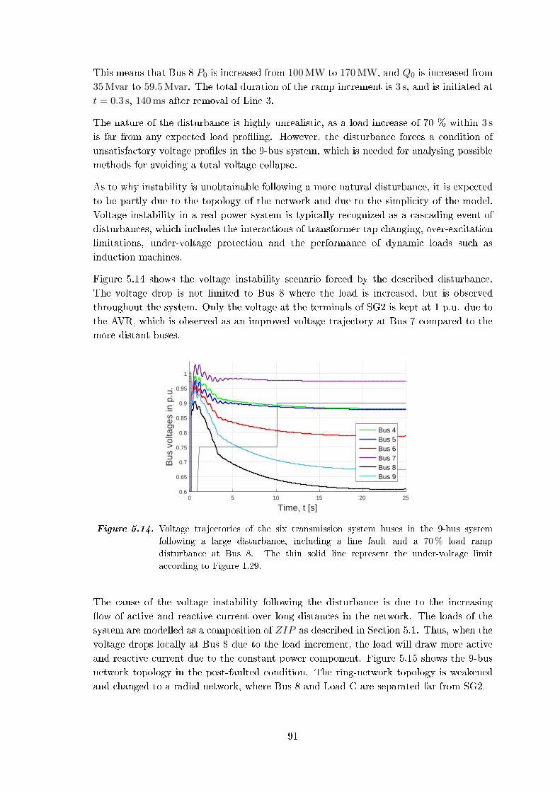
This means that Bus 8 P0 is increased from 100 MW to 170 MW, and Q0 is increased from

35 Mvar to 59.5 Mvar. The total duration of the ramp increment is 3 s, and is initiated at

t = 0.3 s, 140 ms after removal of Line 3.

The nature of the disturbance is highly unrealistic, as a load increase of 70 % within 3 s

is far from any expected load proling. However, the disturbance forces a condition of

unsatisfactory voltage proles in the 9-bus system, which is needed for analysing possible

methods for avoiding a total voltage collapse.

As to why instability is unobtainable following a more natural disturbance, it is expected

to be partly due to the topology of the network and due to the simplicity of the model.

Voltage instability in a real power system is typically recognized as a cascading event of

disturbances, which includes the interactions of transformer tap changing, over-excitation

limitations, under-voltage protection and the performance of dynamic loads such as

induction machines.

Figure 5.14 shows the voltage instability scenario forced by the described disturbance.

The voltage drop is not limited to Bus 8 where the load is increased, but is observed

throughout the system. Only the voltage at the terminals of SG2 is kept at 1 p.u. due to

the AVR, which is observed as an improved voltage trajectory at Bus 7 compared to the

more distant buses.

0 5 10 15 20 25

Time, t [s]

0.6

0.65

0.7

0.75

0.8

0.85

0.9

0.95

1

Bus

vol

tage

s in

p.u

.

Bus 4Bus 5Bus 6Bus 7Bus 8Bus 9

Figure 5.14. Voltage trajectories of the six transmission system buses in the 9-bus system

following a large disturbance, including a line fault and a 70 % load ramp

disturbance at Bus 8. The thin solid line represent the under-voltage limit

according to Figure 1.29.

The cause of the voltage instability following the disturbance is due to the increasing

ow of active and reactive current over long distances in the network. The loads of the

system are modelled as a composition of ZIP as described in Section 5.1. Thus, when the

voltage drops locally at Bus 8 due to the load increment, the load will draw more active

and reactive current due to the constant power component. Figure 5.15 shows the 9-bus

network topology in the post-faulted condition. The ring-network topology is weakened

and changed to a radial network, where Bus 8 and Load C are separated far from SG2.

91

SG2

SG1

A B C

SG3

2 7 5 4 6 9 8

1 3

L2 L1 L6 L5 L4

Figure 5.15. Post-disturbance 9-bus system. The system topology is changed from a ring-

network to a radial string conguration due to the removal of Line 3.

Due to the dynamic excitation inability of SG3 the reactive current is not supplied near

Bus 8, but is injected farther away. Figure 5.16 shows the terminal voltage VT and the

active output current IP,o and the the reactive output current IQ,o of the synchronous

generators. SG3 is unable to keep the voltage at its terminals due to the dynamically

unchanged excitation voltage EG, as shown in Figure 5.12. Due to the drop in terminal

voltage, the reactive power output of SG3 decreases, and the active power output Po is

not increased proportionally with the increase in active output current IP,o. Consequently

more reactive current must be supplied from SG1 and SG2 in order to achieve a new

steady state operating point. The result is that the system voltages, shown in Figure 5.14

are increasingly suppressed when observing the buses in Figure 5.15 from Bus 7 (left)

towards Bus 8 (right).

0 5 10 15 20 25

Time, t [s]

0.65

0.7

0.75

0.8

0.85

0.9

0.95

1

1.05

SG

term

inal

vol

tage

VT in

p.u

.

VT SG1

VT SG2

VT SG3

0 5 10 15 20 25

Time, t [s]

0

0.2

0.4

0.6

0.8

1

1.2

SG

cur

rent

out

put I

o in p

.u. SG1 I

P,o

SG2 IP,o

SG3 IP,o

SG1 IQ,o

SG2 IQ,o

SG3 IQ,o

Figure 5.16. Left: SG terminal voltages. Right: SG active output current IP,o (solid lines), and

reactive current output IQ,o (dotted lines).

5.6.1 Modelling considerations for load-increment in RMS simulations

In Section 5.6 it is described how the IEEE 9-bus system voltages can be forced below the

under-voltage limits by increasing the loading following a large disturbance. In order to

simulate this event with expected system behaviour, it is necessary to add speed governors

to the synchronous generators in the system. Without speed regulation in the modelled

system, even a small increase or decrease in load will eventually make the system unstable,

as the balance between load and generation is unable to recover to an equilibrium.

92

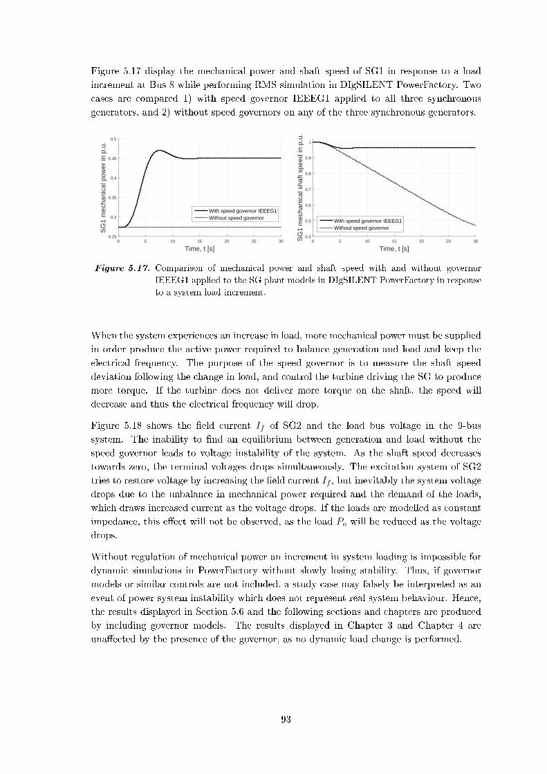
Figure 5.17 display the mechanical power and shaft speed of SG1 in response to a load

increment at Bus 8 while performing RMS simulation in DIgSILENT PowerFactory. Two

cases are compared 1) with speed governor IEEEG1 applied to all three synchronous

generators, and 2) without speed governors on any of the three synchronous generators.

0 5 10 15 20 25 30

Time, t [s]

0.25

0.3

0.35

0.4

0.45

0.5

SG

1 m

echa

nica

l pow

er in

p.u

.

With speed governor IEEEG1Without speed governor

0 5 10 15 20 25 30

Time, t [s]

0.4

0.5

0.6

0.7

0.8

0.9

1

SG

1 m

echa

nica

l sha

ft sp

eed

in p

.u.

With speed governor IEEEG1Without speed governor

Figure 5.17. Comparison of mechanical power and shaft speed with and without governor

IEEEG1 applied to the SG plant models in DIgSILENT PowerFactory in response

to a system load increment.

When the system experiences an increase in load, more mechanical power must be supplied

in order produce the active power required to balance generation and load and keep the

electrical frequency. The purpose of the speed governor is to measure the shaft speed

deviation following the change in load, and control the turbine driving the SG to produce

more torque. If the turbine does not deliver more torque on the shaft, the speed will

decrease and thus the electrical frequency will drop.

Figure 5.18 shows the eld current If of SG2 and the load bus voltage in the 9-bus

system. The inability to nd an equilibrium between generation and load without the

speed governor leads to voltage instability of the system. As the shaft speed decreases

towards zero, the terminal voltages drops simultaneously. The excitation system of SG2

tries to restore voltage by increasing the eld current If , but inevitably the system voltage

drops due to the unbalance in mechanical power required and the demand of the loads,

which draws increased current as the voltage drops. If the loads are modelled as constant

impedance, this eect will not be observed, as the load Po will be reduced as the voltage

drops.

Without regulation of mechanical power an increment in system loading is impossible for

dynamic simulations in PowerFactory without slowly losing stability. Thus, if governor

models or similar controls are not included, a study case may falsely be interpreted as an

event of power system instability which does not represent real system behaviour. Hence,

the results displayed in Section 5.6 and the following sections and chapters are produced

by including governor models. The results displayed in Chapter 3 and Chapter 4 are

unaected by the presence of the governor, as no dynamic load change is performed.

93

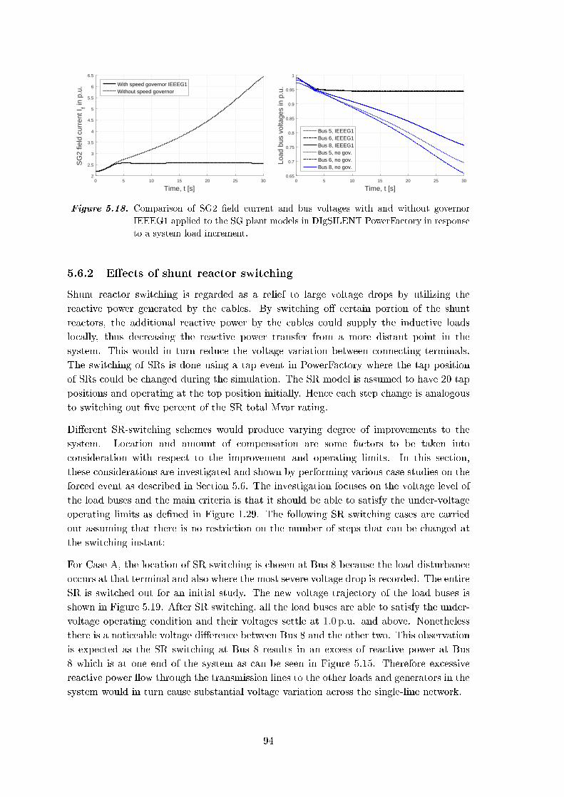
0 5 10 15 20 25 30

Time, t [s]

2

2.5

3

3.5

4

4.5

5

5.5

6

6.5S

G2

field

cur

rent

If in

p.u

. With speed governor IEEEG1Without speed governor

0 5 10 15 20 25 30

Time, t [s]

0.65

0.7

0.75

0.8

0.85

0.9

0.95

1

Load

bus

vol

tage

s in

p.u

.

Bus 5, IEEEG1Bus 6, IEEEG1Bus 8, IEEEG1Bus 5, no gov.Bus 6, no gov.Bus 8, no gov.

Figure 5.18. Comparison of SG2 eld current and bus voltages with and without governor

IEEEG1 applied to the SG plant models in DIgSILENT PowerFactory in response

to a system load increment.

5.6.2 Eects of shunt reactor switching

Shunt reactor switching is regarded as a relief to large voltage drops by utilizing the

reactive power generated by the cables. By switching o certain portion of the shunt

reactors, the additional reactive power by the cables could supply the inductive loads

locally, thus decreasing the reactive power transfer from a more distant point in the

system. This would in turn reduce the voltage variation between connecting terminals.

The switching of SRs is done using a tap event in PowerFactory where the tap position

of SRs could be changed during the simulation. The SR model is assumed to have 20 tap

positions and operating at the top position initially. Hence each step change is analogous

to switching out ve percent of the SR total Mvar rating.

Dierent SR-switching schemes would produce varying degree of improvements to the

system. Location and amount of compensation are some factors to be taken into

consideration with respect to the improvement and operating limits. In this section,

these considerations are investigated and shown by performing various case studies on the

forced event as described in Section 5.6. The investigation focuses on the voltage level of

the load buses and the main criteria is that it should be able to satisfy the under-voltage

operating limits as dened in Figure 1.29. The following SR switching cases are carried

out assuming that there is no restriction on the number of steps that can be changed at

the switching instant:

For Case A, the location of SR switching is chosen at Bus 8 because the load disturbance

occurs at that terminal and also where the most severe voltage drop is recorded. The entire

SR is switched out for an initial study. The new voltage trajectory of the load buses is

shown in Figure 5.19. After SR switching, all the load buses are able to satisfy the under-

voltage operating condition and their voltages settle at 1.0 p.u. and above. Nonetheless

there is a noticeable voltage dierence between Bus 8 and the other two. This observation

is expected as the SR switching at Bus 8 results in an excess of reactive power at Bus

8 which is at one end of the system as can be seen in Figure 5.15. Therefore excessive

reactive power ow through the transmission lines to the other loads and generators in the

system would in turn cause substantial voltage variation across the single-line network.

94

In fact, the new operating voltage of more than 1.2 p.u. at Bus 8 would have otherwise

violated the over-voltage operating limit though it is not covered in the thesis. Hence this

switching case is not considered a viable improvement for the system.

Table 5.3. Denition of switching cases with respective events. All the switching events are

applied at t = 3.019 s. SR4 refers to the shunt reactor that is used to compensate

Line 4. Switching % refers to the compensation amount of that particular SR being

switched out. The rating of each SR can be calculated by dividing the respective line

reactive power values found in Table 4.2 by 2.

Location SR-switching [%] Total Mvar Disconnection [Mvar]

Case A Bus 8 SR4 - 100 183.90

Case BBus 8 SR4 - 50

91.95 + 92.94 = 184.89Bus 4 SR1 - 60

Case CBus 8 SR4 - 45

82.75 + 54.22 + 48.67 = 185.64Bus 5 SR1 - 35

Bus 6 SR6 - 35

0 5 10 15 20 25

Time, t [s]

0.4

0.6

0.8

1

1.2

1.4

Bus

vol

tage

s in

p.u

.

Bus 8Bus 5Bus 6Bus 8, no switchingBus 5, no switchingBus 6, no switching

Figure 5.19. Voltage trajectories of the three load buses with Case A SR switching following a

70 % load ramp disturbance at Bus 8. The trajectories of the non-switching case

is also included for comparison.

The same voltage trajectory curves obtained from Case B and C are presented in Figure

5.20. Referring to Table 5.3, both these cases are used based on the total SR compensation

disconnected of each case in order to match closely with Case A and thus highlighting the

importance of the location. The locations are chosen depending on their proximity with

respect to the load buses. The idea is to distribute the excess reactive power more evenly

and not be transferred from a specic point in the network. It can be observed from

the left side of the gure that the resulting load voltages in Case B are much closer to

one another in comparison with Case A. Moreover, the peak voltage of Bus 8 has been

greatly reduced to a level below 1.04 p.u. indicating a much higher margin from a possible

over-voltage violation.

95

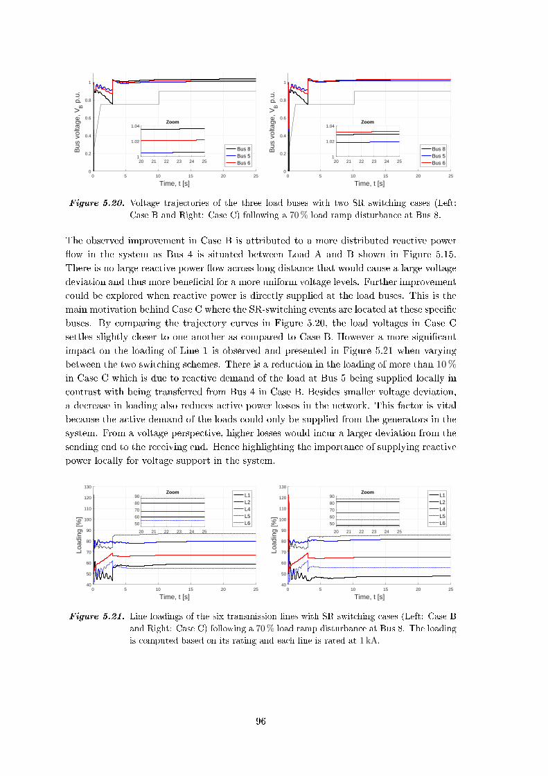
0 5 10 15 20 25

Time, t [s]

0

0.2

0.4

0.6

0.8

1B

us v

olta

ge, V

B p

.u.

Bus 8Bus 5Bus 620 21 22 23 24 25

1

1.02

1.04Zoom

0 5 10 15 20 25

Time, t [s]

0

0.2

0.4

0.6

0.8

1

Bus

vol

tage

, VB p

.u.

Bus 8Bus 5Bus 620 21 22 23 24 25

1

1.02

1.04Zoom

Figure 5.20. Voltage trajectories of the three load buses with two SR switching cases (Left:

Case B and Right: Case C) following a 70 % load ramp disturbance at Bus 8.

The observed improvement in Case B is attributed to a more distributed reactive power

ow in the system as Bus 4 is situated between Load A and B shown in Figure 5.15.

There is no large reactive power ow across long distance that would cause a large voltage

deviation and thus more benecial for a more uniform voltage levels. Further improvement

could be explored when reactive power is directly supplied at the load buses. This is the

main motivation behind Case C where the SR-switching events are located at these specic

buses. By comparing the trajectory curves in Figure 5.20, the load voltages in Case C

settles slightly closer to one another as compared to Case B. However a more signicant

impact on the loading of Line 1 is observed and presented in Figure 5.21 when varying

between the two switching schemes. There is a reduction in the loading of more than 10 %

in Case C which is due to reactive demand of the load at Bus 5 being supplied locally in

contrast with being transferred from Bus 4 in Case B. Besides smaller voltage deviation,

a decrease in loading also reduces active power losses in the network. This factor is vital

because the active demand of the loads could only be supplied from the generators in the

system. From a voltage perspective, higher losses would incur a larger deviation from the

sending end to the receiving end. Hence highlighting the importance of supplying reactive

power locally for voltage support in the system.

0 5 10 15 20 25

Time, t [s]

40

50

60

70

80

90

100

110

120

130

Load

ing

[%]

L1L2L4L5L6

20 21 22 23 24 25

50

60

70

80

90Zoom

0 5 10 15 20 25

Time, t [s]

40

50

60

70

80

90

100

110

120

130

Load

ing

[%]

L1L2L4L5L6

20 21 22 23 24 25

50

60

70

80

90Zoom

Figure 5.21. Line loadings of the six transmission lines with SR switching cases (Left: Case B

and Right: Case C) following a 70 % load ramp disturbance at Bus 8. The loading

is computed based on its rating and each line is rated at 1 kA.

96

5.6.3 Improving the dynamic voltage regulation in the IEEE 9-bus

system

In Section 5.6.2 it is presented how tap switching of SRs can improve the voltage

trajectory following a large disturbance. However, the technical feasibility of implementing

suciently fast and exible SR-switching is an open question. Assuming that cables were

compensated by variable SRs with the ability to regulate within a few seconds, it would

still be natural to consider the SR-switching as an emergency tool in events of collapsing

system voltages. For long HVAC cables, the SRs are dimensioned for several hundreds

Mvar.

Dynamic voltage regulation by including STATCOM

In modern power systems FACTS devices can be implemented (exible AC transmission

systems), such as the static synchronous compensator (STATCOM) or thyristor-controlled

shunt and series devices such as SVC (Static-var-compensator) and TCSC (thyristor

controlled series capacitor). Within their capacity limits these devices provide the ability

to control the voltage and the power factor at a given node in the system independent of

the voltage. However, if the capability limit of the device is reached, it will be voltage

dependent and display similar behaviour as a simple shunt capacitor or reactor, with a

dependency of: Q = V 2/X [2].

In an event of cascading system voltages, a hypothesis is that SR-switching can act as a

recovery tool. Large amounts of reactive power supplied from under-compensated cables

may recover system voltages to satisfy voltage limits. By letting cables inject the majority

of the necessary reactive current, the dependency on FACTS devices may be relieved.

A generic STATCOM model is inserted at Bus 8 in the IEEE 9-bus system. The purpose

is to compare and discuss the combination of SR-switching and improved dynamic voltage

control. A brief discussion of the STATCOM and the PowerFactory model is located in

Appendix G.

Figure 5.22 presents a comparison of the voltage trajectories at Bus 8 with STATCOM

included. It is evident that the presence of STATCOM has a signicant improvement on

the bus voltage. In each case the STATCOM is set to voltage control mode which would

inject or absorb reactive power for dynamic regulation. However, there exists a limit in the

reactive power injection from the STATCOM even though the voltage at the controlled

terminal has not been brought back to its voltage set point which is 1.0 p.u. in this case.

This limit is dependent on the rating of the STATCOM. Hence the gure also illustrates

that a better voltage trajectory is observed in the case of 50 MVA rated STATCOM as

compared to the 25 MVA rated case plus the 0.9 p.u. under-voltage limit is not violated.

97

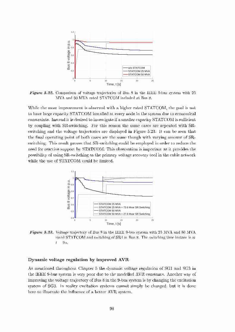
0 5 10 15 20 25

Time, t [s]

0

0.2

0.4

0.6

0.8

1

1.2

Bus

8 v

olta

ge in

p.u

.w/o STATCOMSTATCOM 25 MVASTATCOM 50 MVA

Figure 5.22. Comparison of voltage trajectories of Bus 8 in the IEEE 9-bus system with 25

MVA and 50 MVA rated STATCOM included at Bus 8.

While the most improvement is observed with a higher rated STATCOM, the goal is not

to have large capacity STATCOM installed at every node in the system due to economical

constraints. Instead it is desired to investigate if a smaller capacity STATCOM is sucient

by coupling with SR-switching. For this reason the same cases are repeated with SR-

switching and the voltage trajectories are displayed in Figure 5.23. It can be seen that

the nal operating point of both cases are the same though with varying amount of SR-

switching. This result proves that SR-switching could be employed in order to reduce the

need for reactive support by STATCOM. This observation is important as it provides the

possibility of using SR-switching as the primary voltage recovery tool in the cable network

while the use of STATCOM could be limited.

0 5 10 15 20 25

Time, t [s]

0.4

0.5

0.6

0.7

0.8

0.9

1

1.1

Bus

8 v

olta

ge in

p.u

.

STATCOM 25 MVASTATCOM 25 MVA + 73.6 Mvar SR SwitchingSTATCOM 50 MVASTATCOM 50 MVA + 27.6 Mvar SR Swtiching

Figure 5.23. Voltage trajectory of Bus 8 in the IEEE 9-bus system with 25 MVA and 50 MVA

rated STATCOM and switching of SR4 at Bus 8. The switching time instant is at

t = 9 s.

Dynamic voltage regulation by improved AVR

As mentioned throughout Chapter 5 the dynamic voltage regulation of SG1 and SG3 in

the IEEE 9-bus system is very poor due to the modelled AVR constants. Another way of

improving the voltage trajectory of Bus 8 in the 9-bus system is by changing the excitation

system of SG3. In reality excitation systems cannot simply be changed, but it is done

here to illustrate the inuence of a better AVR system.

98

Figure 5.24 show how the voltage trajectory at Bus 8 is signicantly improved by changing

the AVR system of SG3. The time constants and gains of the excitation system are changed

from the default values in the 9-bus model in DIgSILENT PowerFactory, to the values of

the standard IEEEX1 model.

0 5 10 15 20 25

Time, t [s]

0.6

0.7

0.8

0.9

1

Bu

s 8

vo

lta

ge

in

p.u

.

Default AVR

IEEEX1

IEEEX1 + SR switching

SR tap change

15/20 12/20 11/20

Figure 5.24. Voltage trajectory of Bus 8 in the IEEE 9-bus system with improved excitation

system AVR for SG3 and tap change switching of SR4a located at Bus 8.

When the excitation system is improved, the terminal voltage of SG3 is regulated to 1

p.u. and the SG is able to supply active and reactive power to Bus 8 at lower current.

Hence, improving the AVR system of SG3 changes the power ow of the entire system, as

power to a greater extend is supplied locally.

However, the AVR system regulates the voltage at the terminal of the generator. Hence,

despite being improved, the voltage at the 100 km distant Bus 8 is not regulated back to

its initial voltage.

The voltage at Bus 8 can be regulated close to 1 p.u. by utilizing tap changing of the SRs

connected at Bus 8. Figure 5.24 show a case where the voltage at Bus 8 is regulated to

0.995 p.u. by changing the taps of SR4a at Bus 8 in 3 steps with 3 s between each tap

change. SR4a is rated to 183.9 Mvar, and when divided into 20 taps, each step corresponds

to 9.195 Mvar at 1 p.u.

Figure 5.24 show that even though the AVR systems of SGs are improved, there is still

a need for local voltage control at distant buses. SRs with the capability to dynamically

switch can provide local control.

99

5.7 Summary of voltage stability analysis in the IEEE

9-bus system

This section gives an overview of the large-disturbance voltage stability study carried

out in the IEEE 9-bus system. The following are the conclusions of the voltage stability

analysis based on the 9-bus system:

Conclusions on the modelling procedure:

Load modelling: The voltage instability phenomenon is highly dependent on the

load characteristics. The ∂P/∂V and ∂Q/∂V behaviour of loads will inuence the

ow of active and reactive power in the network, and thus aect the system voltage.

SG reactive power capability limits: Modelling of reactive power capability

limits inuences the power ow of the system and thus the V, P -characteristics of the

network. For realistic representation, V, P -curves should be produced with capability

curves. However, due to the small scale of the 9-bus network, power ow convergence

failure occurs before load-ability dierences can be distinguished between the OHL

base system and the equivalent cable system. For a larger network it is possible

to obtain critical-voltage levels in power ow solutions with capability limits, and

hereby obtain a more meaningful V, P -curve. This is shown in Chapter 6.

Load and generation balance in RMS simulation: Speed governors must be

included in the model in order to avoid system collapse when changing the system

loading in RMS simulations. Without speed governing the inevitable system collapse

may be mistaken for an event of cascading voltage instability.

Excitation system modelling: The dynamic response of excitation systems of

voltage controlled synchronous generators is crucial for the power systems ability

to remain voltage stable. Thus, realistic models of excitation systems and AVR is

necessary for realistic representation of system dynamics.

Conclusions on the voltage stability comparison of OHL systems and equivalent cable

systems:

Load-ability: V, P -characteristics show that the cable based system has higher

load-ability margin Pmax, due to the lower series inductance and resistance resulting

in lower equivalent impedance between generation and load.

SR compensation degree: By under-compensating the cable based system, the

overall load-ability can be increased, as the cables will supply reactive power for

the inductive loads, line inductance and transformers. A consequence of over-

compensating is slightly increased critical voltages due to the overall capacitive

behaviour of the network. However, as discussed by the authors of [40], the load-

ability Pmax in V, P -curves, is more meaningful than the critical voltage.

Voltage trajectories following line faults: When 100 % compensated, the

equivalent cable system displays equal fault response as the OHL base system if

SRs of the faulted line are disconnected. Changing the compensation degree will

induce a dierence in system responses.

100

Switching of shunt reactors: When the 9-bus system is severely weakened by

the removal of a transmission line and an increase in load, the system voltage can be

recovered by switching of shunt reactor capacity. This ability is unavailable in the

OHL base system, where compensation for steady-state operation is unnecessary.

Combining dynamic voltage regulation and SR-switching: Switching of

shunt reactors can aid dynamic voltage regulators such as locally placed FACTS

or AVR systems of SGs. If voltage support in the form of a STATCOM is combined

with SR-switching, the necessary STATCOM capacity may be reduced.

101

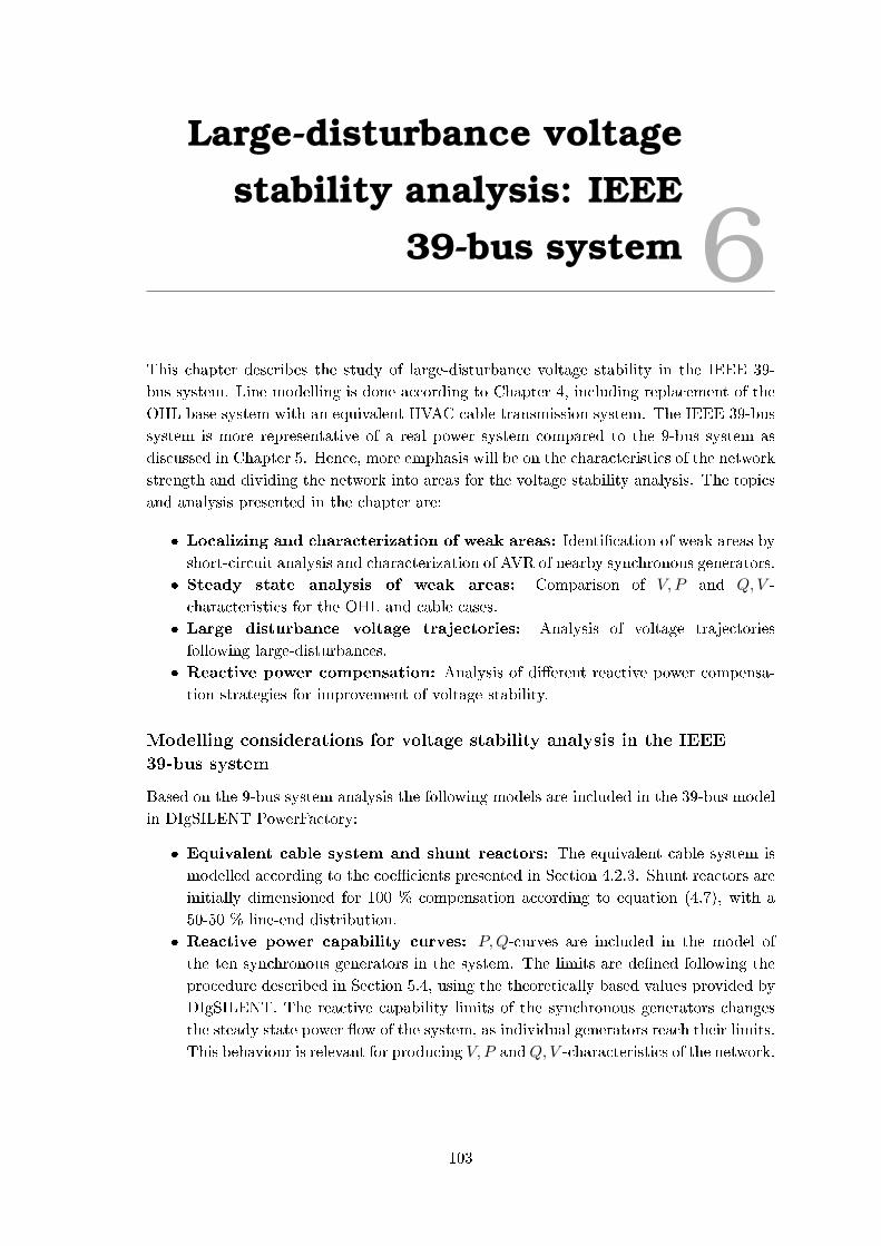
Large-disturbance voltagestability analysis: IEEE

39-bus system 6This chapter describes the study of large-disturbance voltage stability in the IEEE 39-

bus system. Line modelling is done according to Chapter 4, including replacement of the

OHL base system with an equivalent HVAC cable transmission system. The IEEE 39-bus

system is more representative of a real power system compared to the 9-bus system as

discussed in Chapter 5. Hence, more emphasis will be on the characteristics of the network

strength and dividing the network into areas for the voltage stability analysis. The topics

and analysis presented in the chapter are:

Localizing and characterization of weak areas: Identication of weak areas by

short-circuit analysis and characterization of AVR of nearby synchronous generators.

Steady state analysis of weak areas: Comparison of V, P and Q,V -

characteristics for the OHL and cable cases.

Large disturbance voltage trajectories: Analysis of voltage trajectories

following large-disturbances.

Reactive power compensation: Analysis of dierent reactive power compensa-

tion strategies for improvement of voltage stability.

Modelling considerations for voltage stability analysis in the IEEE

39-bus system

Based on the 9-bus system analysis the following models are included in the 39-bus model

in DIgSILENT PowerFactory:

Equivalent cable system and shunt reactors: The equivalent cable system is

modelled according to the coecients presented in Section 4.2.3. Shunt reactors are

initially dimensioned for 100 % compensation according to equation (4.7), with a

50-50 % line-end distribution.

Reactive power capability curves: P,Q-curves are included in the model of

the ten synchronous generators in the system. The limits are dened following the

procedure described in Section 5.4, using the theoretically based values provided by

DIgSILENT. The reactive capability limits of the synchronous generators changes

the steady state power ow of the system, as individual generators reach their limits.

This behaviour is relevant for producing V, P andQ,V -characteristics of the network.

103

Load modelling: Every load in the network is modelled according to the

composition described in Section 5.1. Changing the composition and the ∂P/∂V

and ∂Q/∂V coecients will aect the steady state results as well as the dynamic

behaviour of the network.

Excitation systems: Synchronous generators SG2-SG10 of the IEEE 39-bus

system in DIgSILENT PowerFactory have predened AVR systems. SG1 is excluded

as it represents an external network, rather than an actual synchronous machine.

Each of the AVR system is unique and dynamically responsive, unlike SG1 and SG3

in the 9-bus system. The performance of each excitation system is shown in Figure

6.2.

Speed governors: In order to be able to perform load increments in RMS

simulation each of the synchronous generators are modelled with speed governors,

which are included in the model provided by DIgSILENT.

6.1 Identication and characterization of weak areas in the

IEEE 39-bus system

The voltage stability analysis of the 39-bus system is limited to a few selected network

areas. Thus, a short-circuit analysis is performed in DIgSILENT PowerFactory with the

purpose of calculating the apparent short-circuit power at each load bus in the network.

The strength of a power system node (in a SG based system) is a combination of the

Thevenin equivalent impedance Zth seen from the node, and the mechanical inertia J

of nearby generation units [2]. Hence, a weak node or area is characterized by a high

Thevenin impedance and low mechanical inertia. In relation to voltage stability analysis,

a low short-circuit power at a load bus indicate a possible large impedance between the

load and the generating units. Thus, short-circuit power is an indicator of the distance

between the load and generation, and as such provides information regarding the V, P -

characteristics and the voltage sensitivity to load increments.

Table 6.1 show the results of the short-circuit calculations. The calculations are performed

for the equivalent cable case with 100 % compensation. Thus, all lines are modelled

according to the scaling coecients presented in Section 4.2.3. The equivalent cable case

display slightly larger short-circuit powers SSC , due to the lower line resistance and line

inductance in comparison to the OHL base case. However, the overall relative strength

between the buses and areas remain unchanged.

SG1, which is feeding Bus 39, displays a very large short-circuit power in comparison

to the other buses. This is because SG1 is modelled to represent the interconnection

between the New England power system and the rest of USA and Canada. For the same

reason, SG1 is modelled without any AVR system, whereas the remaining 9 synchronous

generators have individual AVR models.

Based on the short-circuit results, the load buses of the system are divided into areas

from A to G based on their short-circuit power and their location in the network. Area A

represent the grouping of load buses in close proximity displaying the highest short-circuit

powers. While, Area G represent the grouping of load buses in close proximity displaying

the lowest short-circuit powers.

104

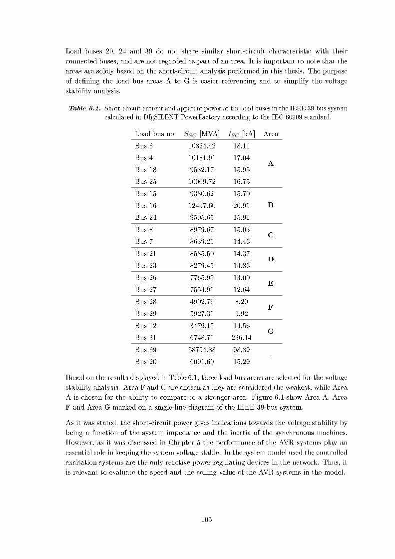
Load buses 20, 24 and 39 do not share similar short-circuit characteristic with their

connected buses, and are not regarded as part of an area. It is important to note that the

areas are solely based on the short-circuit analysis performed in this thesis. The purpose

of dening the load bus areas A to G is easier referencing and to simplify the voltage

stability analysis.

Table 6.1. Short-circuit current and apparent power at the load buses in the IEEE 39-bus system

calculated in DIgSILENT PowerFactory according to the IEC 60909 standard.

Load bus no. SSC [MVA] ISC [kA] Area

Bus 3 10824.42 18.11

ABus 4 10181.91 17.04

Bus 18 9532.17 15.95

Bus 25 10009.72 16.75

Bus 15 9380.62 15.70

BBus 16 12497.60 20.91

Bus 24 9505.65 15.91

Bus 8 8979.67 15.03C

Bus 7 8639.21 14.46

Bus 21 8585.50 14.37D

Bus 23 8279.45 13.86

Bus 26 7765.95 13.00E

Bus 27 7553.91 12.64

Bus 28 4902.76 8.20F

Bus 29 5927.31 9.92

Bus 12 3479.15 14.56G

Bus 31 6748.71 236.14

Bus 39 58794.88 98.39-

Bus 20 6091.60 15.29

Based on the results displayed in Table 6.1, three load bus areas are selected for the voltage

stability analysis. Area F and G are chosen as they are considered the weakest, while Area

A is chosen for the ability to compare to a stronger area. Figure 6.1 show Area A, Area

F and Area G marked on a single-line diagram of the IEEE 39-bus system.

As it was stated, the short-circuit power gives indications towards the voltage stability by

being a function of the system impedance and the inertia of the synchronous machines.

However, as it was discussed in Chapter 5 the performance of the AVR systems play an

essential role in keeping the system voltage stable. In the system model used the controlled

excitation systems are the only reactive power regulating devices in the network. Thus, it

is relevant to evaluate the speed and the ceiling value of the AVR systems in the model.

105

3725

30

2

39

9

26

18

3

4

5

7

8

17

14

6

3111

10

32

12

13

15

16

2728

29

3824

35

21 22

23

36

33

19

20

Busbar

Transfomer

Generator

1

34

SG10

SG8

SG1

SG2SG3

SG5 SG4

SG7

SG9

SG6

Area G

Area F

Area A

Figure 6.1. Single-line diagram of the New England IEEE 39-bus system with marking of the

Areas A, F and G.

Figure 6.2 show the excitation voltage response of the synchronous generators in the

system when in turn exposed to a three-phase fault located at 1 % line distance from the

respective SG.

0.5 1 1.5 2 2.5 3 3.5 4 4.5 5

Time, t [s]

1

2

3

4

5

6

SG

exc

itatio

n vo

ltage

in p

.u.

SG1SG2SG3SG4SG5SG6SG7SG8SG9SG10

Figure 6.2. Excitation response of the synchronous generators in the IEEE 39-bus system

following a permanent three-phase short-circuit located at 1 % line distance from

each SG respectively.

SG3, which is located in Area G, displays the lowest excitation voltage EG ceiling value

compared to the other machines. SG2, also located in Area G, has an average ceiling

value. Neither of the two reaches their ceiling values fast in comparison to the excitation

systems of the other machines. SG9, which is located in Area F, has the highest ceiling

value of the excitation systems. The dependency of excitation system controls will not be

expressed in the V, P and Q,V -curves produced by steady state analysis, but will inuence

the dynamic voltage trajectory analysis.

106

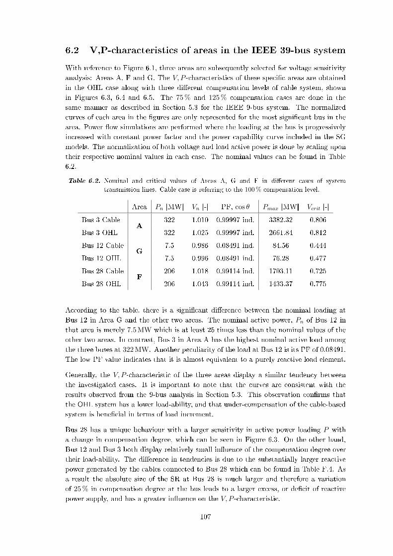
6.2 V,P-characteristics of areas in the IEEE 39-bus system

With reference to Figure 6.1, three areas are subsequently selected for voltage sensitivity

analysis: Areas A, F and G. The V, P -characteristics of these specic areas are obtained

in the OHL case along with three dierent compensation levels of cable system, shown

in Figures 6.3, 6.4 and 6.5. The 75 % and 125 % compensation cases are done in the

same manner as described in Section 5.3 for the IEEE 9-bus system. The normalized

curves of each area in the gures are only represented for the most signicant bus in the

area. Power ow simulations are performed where the loading at the bus is progressively

increased with constant power factor and the power capability curve included in the SG

models. The normalization of both voltage and load active power is done by scaling upon

their respective nominal values in each case. The nominal values can be found in Table

6.2.

Table 6.2. Nominal and critical values of Areas A, G and F in dierent cases of system

transmission lines. Cable case is referring to the 100 % compensation level.

Area Pn [MW] Vn [-] PF, cos θ Pmax [MW] Vcrit [-]

Bus 3 CableA

322 1.010 0.99997 ind. 3382.32 0.806

Bus 3 OHL 322 1.025 0.99997 ind. 2661.84 0.812

Bus 12 CableG

7.5 0.986 0.08491 ind. 84.56 0.444

Bus 12 OHL 7.5 0.996 0.08491 ind. 76.28 0.477

Bus 28 CableF

206 1.018 0.99114 ind. 1703.11 0.725

Bus 28 OHL 206 1.043 0.99114 ind. 1433.37 0.775

According to the table, there is a signicant dierence between the nominal loading at

Bus 12 in Area G and the other two areas. The nominal active power, Pn of Bus 12 in

that area is merely 7.5 MW which is at least 25 times less than the nominal values of the

other two areas. In contrast, Bus 3 in Area A has the highest nominal active load among

the three buses at 322 MW. Another peculiarity of the load at Bus 12 is its PF of 0.08491.

The low PF value indicates that it is almost equivalent to a purely reactive load element.

Generally, the V, P -characteristic of the three areas display a similar tendency between

the investigated cases. It is important to note that the curves are consistent with the

results observed from the 9-bus analysis in Section 5.3. This observation conrms that

the OHL system has a lower load-ability, and that under-compensation of the cable-based

system is benecial in terms of load increment.

Bus 28 has a unique behaviour with a larger sensitivity in active power loading P with

a change in compensation degree, which can be seen in Figure 6.3. On the other hand,

Bus 12 and Bus 3 both display relatively small inuence of the compensation degree over

their load-ability. The dierence in tendencies is due to the substantially larger reactive

power generated by the cables connected to Bus 28 which can be found in Table F.4. As

a result the absolute size of the SR at Bus 28 is much larger and therefore a variation

of 25 % in compensation degree at the bus leads to a larger excess, or decit of reactive

power supply, and has a greater inuence on the V, P -characteristic.

107

0 1 2 3 4 5 6 7 8 9 10

Load active power, P/Pn

0.6

0.65

0.7

0.75

0.8

0.85

0.9

0.95

1

1.05

Nor

mal

ized

bus

vol

tage

, V/V

n

Cable, 100 % compensationCable, 75 % compensationCable, 125 % compensationOHL

Figure 6.3. Normalized V, P -characteristic of Bus 28 in Area F in four dierent cases of system

transmission lines and reactive power compensation degree.

0 2 4 6 8 10 12

Load active power, P/Pn

0.3

0.4

0.5

0.6

0.7

0.8

0.9

1

1.1

Nor

mal

ized

bus

vol

tage

, V/V

n

Cable, 100 % compensationCable, 75 % compensationCable, 125 % compensationOHL

Figure 6.4. Normalized V, P -characteristic of Bus 12 in Area G in four dierent cases of system

transmission lines and reactive power compensation degree.

0 2 4 6 8 10 12

Load active power, P/Pn

0.65

0.7

0.75

0.8

0.85

0.9

0.95

1

1.05

Nor

mal

ized

bus

vol

tage

, V/V

n

Cable, 100 % compensationCable, 75 % compensationCable, 125 % compensationOHL

Figure 6.5. Normalized V, P -characteristic of Bus 3 in Area A in four dierent cases of system

transmission lines and reactive power compensation degree.

108

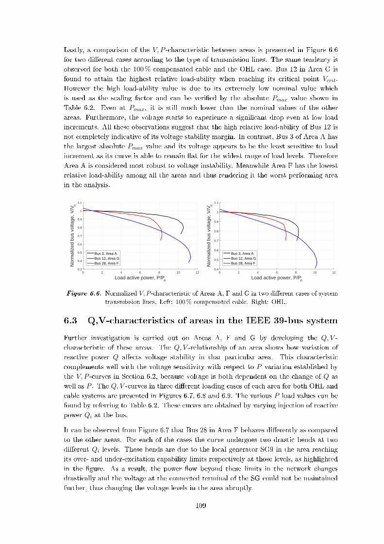
Lastly, a comparison of the V, P -characteristic between areas is presented in Figure 6.6

for two dierent cases according to the type of transmission lines. The same tendency is

observed for both the 100 % compensated cable and the OHL case. Bus 12 in Area G is

found to attain the highest relative load-ability when reaching its critical point Vcrit.

However the high load-ability value is due to its extremely low nominal value which

is used as the scaling factor and can be veried by the absolute Pmax value shown in

Table 6.2. Even at Pmax, it is still much lower than the nominal values of the other

areas. Furthermore, the voltage starts to experience a signicant drop even at low load

increments. All these observations suggest that the high relative load-ability of Bus 12 is

not completely indicative of its voltage stability margin. In contrast, Bus 3 of Area A has

the largest absolute Pmax value and its voltage appears to be the least sensitive to load

increment as its curve is able to remain at for the widest range of load levels. Therefore

Area A is considered most robust to voltage instability. Meanwhile Area F has the lowest

relative load-ability among all the areas and thus rendering it the worst performing area

in the analysis.

0 2 4 6 8 10 12

Load active power, P/Pn

0.3

0.4

0.5

0.6

0.7

0.8

0.9

1

1.1

Nor

mal

ized

bus

vol

tage

, V/V

n

Bus 3, Area ABus 12, Area GBus 28, Area F

0 2 4 6 8 10 12

Load active power, P/Pn

0.4

0.5

0.6

0.7

0.8

0.9

1

1.1

Nor

mal

ized

bus

vol

tage

, V/V

n

Bus 3, Area ABus 12, Area GBus 28, Area F

Figure 6.6. Normalized V, P -characteristic of Areas A, F and G in two dierent cases of system

transmission lines. Left: 100 % compensated cable. Right: OHL.

6.3 Q,V-characteristics of areas in the IEEE 39-bus system

Further investigation is carried out on Areas A, F and G by developing the Q,V -

characteristic of these areas. The Q,V -relationship of an area shows how variation of

reactive power Q aects voltage stability in that particular area. This characteristic

complements well with the voltage sensitivity with respect to P variation established by

the V, P -curves in Section 6.2, because voltage is both dependent on the change of Q as

well as P . The Q,V -curves in three dierent loading cases of each area for both OHL and

cable systems are presented in Figures 6.7, 6.8 and 6.9. The various P load values can be

found by referring to Table 6.2. These curves are obtained by varying injection of reactive

power Qi at the bus.

It can be observed from Figure 6.7 that Bus 28 in Area F behaves dierently as compared

to the other areas. For each of the cases the curve undergoes two drastic bends at two

dierent Qi levels. These bends are due to the local generator SG9 in the area reaching

its over- and under-excitation capability limits respectively at those levels, as highlighted

in the gure. As a result, the power ow beyond these limits in the network changes

drastically and the voltage at the connected terminal of the SG could not be maintained

further, thus changing the voltage levels in the area abruptly.

109

0.4 0.5 0.6 0.7 0.8 0.9 1 1.1 1.2 1.3 1.4

Bus 28 voltage in p.u.

-1000

-500

0

500

1000

1500

2000

Inje

cte

dre

active

po

we

r,Q

i[M

va

r]

Pn, cable

5Pn, cable

Pmax

, cable

Pn, OHL

5Pn, OHL

Pmax

, OHL

SG9 Under-excitation

limit reached

SG9 Over-excitation

limit reached

Figure 6.7. Q,V -characteristic of Area F in three dierent loading levels for both OHL and

cable systems. Dotted line refers to the OHL case.

0.3 0.4 0.5 0.6 0.7 0.8 0.9 1 1.1 1.2 1.3

Bus 12 voltage in p.u.

-1000

-500

0

500

1000

1500

2000

2500

Inje

cted

rea

ctiv

e po

wer

, Qi [M

var]

Pn, cable

5Pn, cable

Pmax

, cable

Pn, OHL

5Pn, OHL

Pmax

, OHL

Figure 6.8. Q,V -characteristic of Area G in three dierent loading levels for both OHL and

cable systems. Dotted line refers to the OHL case.

0.7 0.8 0.9 1 1.1 1.2 1.3

Bus 3 voltage in p.u.

-2000

-1000

0

1000

2000

3000

Inje

cted

rea

ctiv

e po

wer

, Qi [M

var]

Pn, cable

5Pn, cable

Pmax

, cable

Pn, OHL

5Pn, OHL

Pmax

, OHL

Figure 6.9. Q,V -characteristic of Area A in three dierent loading levels for both OHL and

cable systems. Dotted line refers to the OHL case.

110

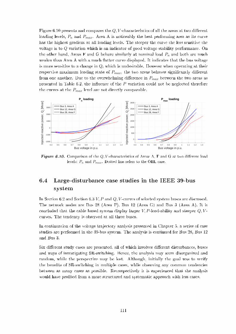
Figure 6.10 presents and compares the Q,V -characteristics of all the areas at two dierent

loading levels, Pn and Pmax. Area A is noticeably the best performing area as its curve

has the highest gradient at all loading levels. The steeper the curve the less sensitive the

voltage is to Q variation which is an indicator of good voltage stability performance. On

the other hand, Areas F and G behave similarly at nominal load Pn and both are much

weaker than Area A with a much atter curve displayed. It indicates that the bus voltage

is more sensitive to a change in Qi which is undesirable. However when operating at their

respective maximum loading state of Pmax, the two areas behaves signicantly dierent

from one another. Due to the overwhelming dierence in Pmax between the two areas as

presented in Table 6.2, the inuence of the P variation could not be neglected therefore

the curves at the Pmax level are not directly comparable.

0.4 0.5 0.6 0.7 0.8 0.9 1 1.1 1.2 1.3 1.4

Bus voltage in p.u.

-2000

-1000

0

1000

2000

3000

Inje

cted

rea

ctiv

e po

wer

, Qi [M

var]

Pn loading

Bus 3, Area ABus 12, Area GBus 28, Area F

0.3 0.4 0.5 0.6 0.7 0.8 0.9 1 1.1 1.2 1.3

Bus voltage in p.u.

0

500

1000

1500

2000

2500

3000

Inje

cted

rea

ctiv

e po

wer

, Qi [M

var]

Pmax

loading

Bus 3, Area ABus 12, Area GBus 28, Area F

Figure 6.10. Comparison of the Q,V -characteristics of Areas A, F and G at two dierent load

levels: Pn and Pmax. Dotted line refers to the OHL case.

6.4 Large-disturbance case studies in the IEEE 39-bus

system

In Section 6.2 and Section 6.3 V, P and Q,V -curves of selected system buses are discussed.

The network nodes are Bus 28 (Area F), Bus 12 (Area G) and Bus 3 (Area A). It is

concluded that the cable based system display larger V, P -load-ability and steeper Q,V -

curves. The tendency is observed at all three buses.

In continuation of the voltage trajectory analysis presented in Chapter 5, a series of case

studies are performed in the 39-bus system. The analysis is continued for Bus 28, Bus 12

and Bus 3.

Six dierent study cases are presented, all of which involves dierent disturbances, buses

and ways of investigating SR-switching. Hence, the analysis may seem disorganized and

random, while the perspective may be lost. Although, initially the goal was to verify

the benets of SR-switching in multiple cases, while observing any common tendencies

between as many cases as possible. Retrospectively it is experienced that the analysis

would have proted from a more structured and systematic approach with less cases.

111

Properties of SR-switching

The focus is on improving the system voltages following large disturbances by utilizing

SR-switching. It is desired to investigate if SR-switching can be improved and generalized

for large-disturbances with respect to three properties:

1. Amount: The necessary amount (i.e. quantity) of switched shunt reactor capacity

Qsw necessary for voltage recovery at a given bus or area.

2. Location: Procedural switching of SRs in the area of and in the proximity of the

most weakened bus (i.e. lowest voltage bus).

3. Timing: Timing of the necessary shunt reactor switching Qsw with respect to

satisfying both under-voltage and over-voltage trajectory limits (i.e. limiting

temporary voltage over-shoot).

Although SR-switching is to be improved for these properties, an actual optimization is

not performed. Instead, the goal is to provide pointers towards guidelines and future work

within SR-switching for improved voltage stability in large-disturbance events. Thus, the

study cases are designed to imitate large-disturbances in the network, while investigating

possible tendencies towards the mentioned properties.

The study cases involves a combination of one or more of the following disturbances:

Pre-disturbance steady-state load increase to simulate a high-load condition.

Dynamic load ramp in specic areas to simulate load-restoration.

Switching of transmission lines to simulate events of over-loading.

Switching of transmission lines in the event of permanent faults.

Loss of generation due to permanent faults near generation units.

Each large-disturbance study case is designed to involve at least one of the discussed areas:

Area A, Area F and Area G.

6.4.1 Large-disturbance Case 1: Dynamic load increase, loss of

generation and transformer in Area G

The area of interest in this case is Area G with reference to Figure 6.1. The large-

disturbance is applied in the form of sequential events as follow:

Load ramp increase of 50 % in the area over a duration of 10 s starting from t = 0.1 s.

Three-phase fault at the terminal bus of SG3, t = 4 s.

Permanent disconnection of SG3 and transformer, t = 4.06 s.

Permanent disconnection of Transformer 12-13, t = 7.0 s.

The outcome of the described disturbance can be seen by the bus voltages in the area

in Figure 6.11. There are certain buses that are not shown in the gure as they display

similar characteristics. The voltage trajectory of Bus 12 ends at a level below the under-

voltage limit thus violating continuous operating conditions. Two SR-switching schemes

are introduced to keep the voltages above the limit and to recover back to approximately

1.0 p.u. The two schemes are basically the same in terms of the amount and location

of switching. However, one is an instantaneous switching where the entire quantity

is switched out instantly, whereas the other alternative divides the switching into two

separate instants. The SR-switching events are shown in Table 6.3.

112

The eects of both SR-switching schemes can be seen in Figure 6.11. It is observed that

the resulting nal operating states of both schemes are identical. This is due to the same

amount being disconnected at the same location, and thus the resulting power ow in

the system is equal. Nevertheless, there is a signicant dierence in the peak voltage at

Bus 11 between them. The instantaneous switching produces an overshoot value of over

1.1 p.u. while it is limited below 1.07 p.u. with the progressive one. This observation

indicates that it is more advantageous to distribute the SR-switching amount into a few

instants which results in a higher tolerance margin from the over-voltage limits.

There still appears to be a substantial voltage dierence between Bus 12 and Bus 11 even

after SR switching. This is because the two terminals are connected via a transformer,

and no reactive power is supplied by cables directly at Bus 12. Hence no SR-switching

could be carried out to compensate the voltage drop across the transformer.

5 10 15 20 25 30

Time, t [s]

0.85

0.9

0.95

1

1.05

1.1

Are

a G

bus v

oltages in p

.u.

Bus 12, prog. SR sw.

Bus 11, prog. SR sw.

Bus 12, instant SR sw.

Bus 11, instant SR sw.

Bus 12, no SR sw.

Bus 11, no SR sw.

1

2

Figure 6.11. Voltage trajectories of Bus 12 and Bus 11 in Area G for large-disturbance Case 1.

Number indicates the switching sequence according to Table 6.3.

6.4.2 Large-disturbance Case 2: Fault and loss of generation in Area G

This study case is centred around Area G with reference to Figure 6.1. The study case

is carried out for 25 % increased steady-state loading, such that P = 1.25Pn at all load

buses in the system. The power factor is kept constant. The events of the disturbance

are:

Three-phase fault at the terminal bus of SG3, t = 1 s.

Permanent disconnection of SG3 and transformer, t = 1.060 s.

Permanent disconnection of Line 13-14 and shunt reactors due to overloading, t = 3 s.

Permanent disconnection of transformer at SG2 due to overloading, t = 4 s.

SR-switching with the purpose of voltage recovery is initiated at t = 6 s. Figure 6.12 show

a sensitivity of switching either 25 %, 50 %, 75% or 100% of the available QSR amount in

Area G, when accounting for the SRs taken out of service due to line disconnection. As

expected, the voltage recovers to an increasing value as more reactive power is switched

Qsw. However, in this case, 100 % SR-switching in Area G is insucient for full voltage

recovery. Due to the nature of the disturbance, the neighbouring buses in Area C are

aected by the event and requires compensation as well as Area G.

113

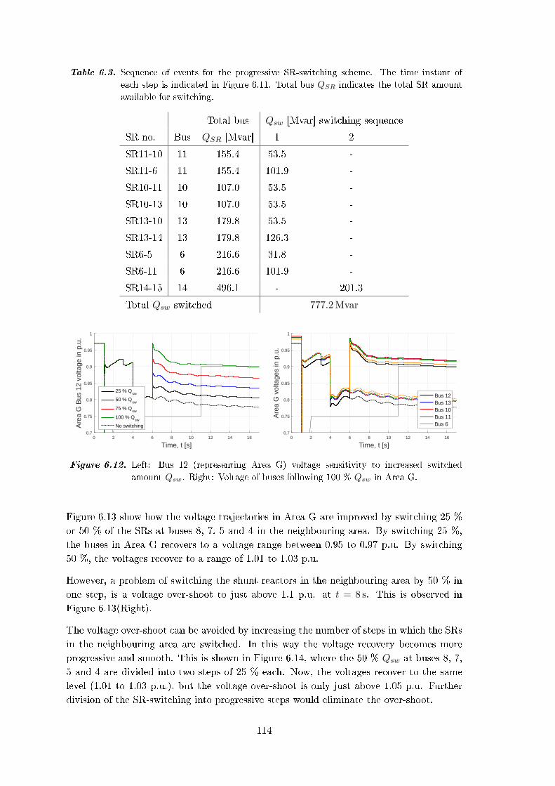
Table 6.3. Sequence of events for the progressive SR-switching scheme. The time instant of

each step is indicated in Figure 6.11. Total bus QSR indicates the total SR amount

available for switching.

Total bus Qsw [Mvar] switching sequence

SR no. Bus QSR [Mvar] 1 2

SR11-10 11 155.4 53.5 -

SR11-6 11 155.4 101.9 -

SR10-11 10 107.0 53.5 -

SR10-13 10 107.0 53.5 -

SR13-10 13 179.8 53.5 -

SR13-14 13 179.8 126.3 -

SR6-5 6 216.6 31.8 -

SR6-11 6 216.6 101.9 -

SR14-15 14 496.1 - 201.3

Total Qsw switched 777.2 Mvar

0 2 4 6 8 10 12 14 16

Time, t [s]

0.7

0.75

0.8

0.85

0.9

0.95

1

Are

a G

Bus

12

volta

ge in

p.u

.

25 % Qsw

50 % Qsw

75 % Qsw

100 % Qsw

No switching

0 2 4 6 8 10 12 14 16

Time, t [s]

0.7

0.75

0.8

0.85

0.9

0.95

1

Are

a G

vol

tage

s in

p.u

.

Bus 12Bus 13Bus 10Bus 11Bus 6

Figure 6.12. Left: Bus 12 (representing Area G) voltage sensitivity to increased switched

amount Qsw. Right: Voltage of buses following 100 % Qsw in Area G.

Figure 6.13 show how the voltage trajectories in Area G are improved by switching 25 %

or 50 % of the SRs at buses 8, 7, 5 and 4 in the neighbouring area. By switching 25 %,

the buses in Area G recovers to a voltage range between 0.95 to 0.97 p.u. By switching

50 %, the voltages recover to a range of 1.01 to 1.03 p.u.

However, a problem of switching the shunt reactors in the neighbouring area by 50 % in

one step, is a voltage over-shoot to just above 1.1 p.u. at t = 8 s. This is observed in

Figure 6.13(Right).

The voltage over-shoot can be avoided by increasing the number of steps in which the SRs

in the neighbouring area are switched. In this way the voltage recovery becomes more

progressive and smooth. This is shown in Figure 6.14, where the 50 % Qsw at buses 8, 7,

5 and 4 are divided into two steps of 25 % each. Now, the voltages recover to the same

level (1.01 to 1.03 p.u.), but the voltage over-shoot is only just above 1.05 p.u. Further

division of the SR-switching into progressive steps would eliminate the over-shoot.

114

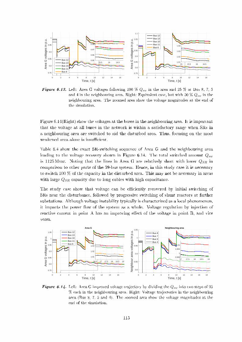
0 2 4 6 8 10 12 14 16

Time, t [s]

0.75

0.8

0.85

0.9

0.95

1

Are

a G

vol

tage

s in

p.u

.

Bus 12Bus 13Bus 10Bus 11Bus 6

15.5 16 16.50.95

0.96

0.97

0.98

0 2 4 6 8 10 12 14 16

Time, t [s]

0.75

0.8

0.85

0.9

0.95

1

1.05

1.1

Are

a G

vol

tage

s in

p.u

.

Bus 12Bus 13Bus 10Bus 11Bus 6

15 15.5 16 16.51.01

1.02

1.03

1.04

Figure 6.13. Left: Area G voltages following 100 % Qsw in the area and 25 % at Bus 8, 7, 5

and 4 in the neighbouring area. Right: Equivalent case, but with 50 % Qsw in the

neighbouring area. The zoomed area show the voltage magnitudes at the end of

the simulation.

Figure 6.14(Right) show the voltages at the buses in the neighbouring area. It is important

that the voltage at all buses in the network is within a satisfactory range when SRs in

a neighbouring area are switched to aid the disturbed area. Thus, focusing on the most

weakened area alone is insucient.

Table 6.4 show the exact SR-switching sequence of Area G and the neighbouring area

leading to the voltage recovery shown in Figure 6.14. The total switched amount Qswis 1125 Mvar. Noting that the lines in Area G are relatively short with lower QSR in

comparison to other parts of the 39-bus system. Hence, in this study case it is necessary

to switch 100 % of the capacity in the disturbed area. This may not be necessary in areas

with large QSR capacity due to long cables with high capacitance.

The study case show that voltage can be eciently recovered by initial switching of

SRs near the disturbance, followed by progressive switching of shunt reactors at farther

substations. Although voltage instability typically is characterized as a local phenomenon,

it impacts the power ow of the system as a whole. Voltage regulation by injection of

reactive current in point A has an improving eect of the voltage in point B, and vice

versa.

0 2 4 6 8 10 12 14 16

Time, t [s]

0.75

0.8

0.85

0.9

0.95

1

1.05

Are

a G

vol

tage

s in

p.u

.

Area G

Bus 12Bus 13Bus 10Bus 11Bus 6

16.5 17 17.5 18 18.5 19

1.01

1.02

1.03

0 2 4 6 8 10 12 14 16 18

Time, t [s]

0.8

0.85

0.9

0.95

1

1.05

Nei

ghbo

ur a

rea

volta

ges

in p

.u.

Neighbouring area

Bus 8Bus 7Bus 5Bus 4

17 17.5 18 18.5 190.995

1

1.005

1.01

Figure 6.14. Left: Area G improved voltage trajectory by dividing the Qsw into two steps of 25

% each in the neighbouring area. Right: Voltage trajectories in the neighbouring

area (Bus 8, 7, 5 and 4). The zoomed area show the voltage magnitudes at the

end of the simulation.

115

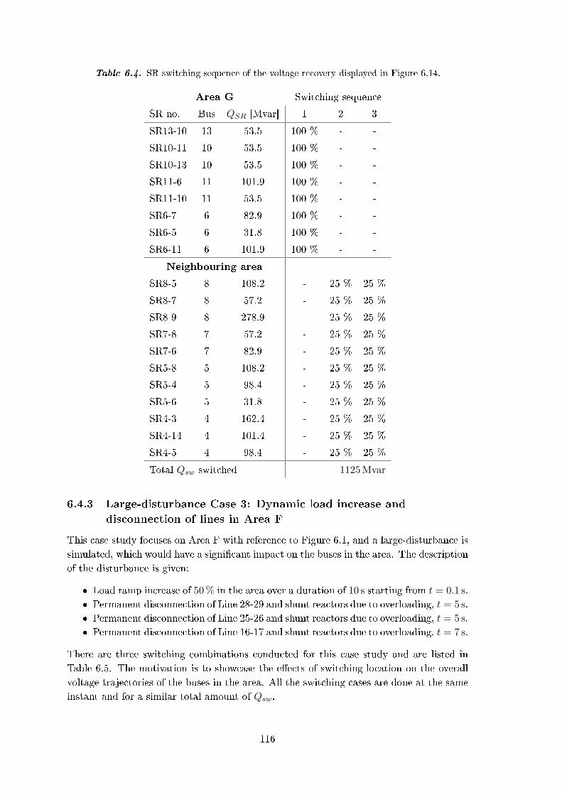
Table 6.4. SR switching sequence of the voltage recovery displayed in Figure 6.14.

Area G Switching sequence

SR no. Bus QSR [Mvar] 1 2 3

SR13-10 13 53.5 100 % - -

SR10-11 10 53.5 100 % - -

SR10-13 10 53.5 100 % - -

SR11-6 11 101.9 100 % - -

SR11-10 11 53.5 100 % - -

SR6-7 6 82.9 100 % - -

SR6-5 6 31.8 100 % - -

SR6-11 6 101.9 100 % - -

Neighbouring area

SR8-5 8 108.2 - 25 % 25 %

SR8-7 8 57.2 - 25 % 25 %

SR8-9 8 278.9 - 25 % 25 %

SR7-8 7 57.2 - 25 % 25 %

SR7-6 7 82.9 - 25 % 25 %

SR5-8 5 108.2 - 25 % 25 %

SR5-4 5 98.4 - 25 % 25 %

SR5-6 5 31.8 - 25 % 25 %

SR4-3 4 162.4 - 25 % 25 %

SR4-14 4 101.4 - 25 % 25 %

SR4-5 4 98.4 - 25 % 25 %

Total Qsw switched 1125 Mvar

6.4.3 Large-disturbance Case 3: Dynamic load increase and

disconnection of lines in Area F

This case study focuses on Area F with reference to Figure 6.1, and a large-disturbance is

simulated, which would have a signicant impact on the buses in the area. The description

of the disturbance is given:

Load ramp increase of 50 % in the area over a duration of 10 s starting from t = 0.1 s.

Permanent disconnection of Line 28-29 and shunt reactors due to overloading, t = 5 s.

Permanent disconnection of Line 25-26 and shunt reactors due to overloading, t = 5 s.

Permanent disconnection of Line 16-17 and shunt reactors due to overloading, t = 7 s.

There are three switching combinations conducted for this case study and are listed in

Table 6.5. The motivation is to showcase the eects of switching-location on the overall

voltage trajectories of the buses in the area. All the switching cases are done at the same

instant and for a similar total amount of Qsw.

116

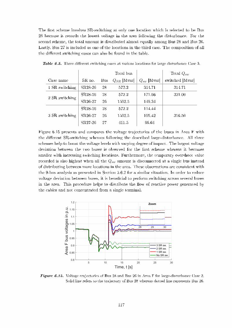
The rst scheme involves SR-switching at only one location which is selected to be Bus

28 because it records the lowest voltage in the area following the disturbance. For the

second scheme, the total amount is distributed almost equally among Bus 28 and Bus 26.

Lastly, Bus 27 is included as one of the locations in the third case. The composition of all

the dierent switching cases can also be found in the table.

Table 6.5. Three dierent switching cases at various locations for large-disturbance Case 3.

Total bus Total Qsw

Case name SR no. Bus QSR [Mvar] Qsw [Mvar] switched [Mvar]

1 SR switching SR28-26 28 572.2 314.71 314.71

2 SR switchingSR28-26 28 572.2 171.66 321.00

SR26-27 26 1502.5 149.34

3 SR switching

SR28-26 28 572.2 114.44

SR26-27 26 1502.5 105.42 316.50

SR27-26 27 411.5 96.64

Figure 6.15 presents and compares the voltage trajectories of the buses in Area F with

the dierent SR-switching schemes following the described large-disturbance. All three

schemes help to boost the voltage levels with varying degree of impact. The largest voltage

deviation between the two buses is observed for the rst scheme whereas it becomes

smaller with increasing switching locations. Furthermore, the temporary overshoot value

recorded is also highest when all the Qsw amount is disconnected at a single bus instead

of distributing between more locations in the area. These observations are consistent with

the 9-bus analysis as presented in Section 5.6.2 for a similar situation. In order to reduce

voltage deviation between buses, it is benecial to perform switching across several buses

in the area. This procedure helps to distribute the ow of reactive power generated by

the cables and not concentrated from a single terminal.

5 10 15 20 25 30

Time, t [s]

0.8

0.85

0.9

0.95

1

1.05

1.1

1.15

1.2

Are

a F

bus v

oltages in p

.u.

3 SR sw.

2 SR sw.

1 SR sw.

No SR sw.

28 29 30

Zoom

Figure 6.15. Voltage trajectories of Bus 28 and Bus 26 in Area F for large-disturbance Case 2.

Solid line refers to the trajectory of Bus 28 whereas dotted line represents Bus 26.

117

6.4.4 Large-disturbance Case 4: Transmission line over-loading in

Area A

This study case is centred around Area A with reference to Figure 6.1. The study case

is carried out for 25 % increased steady-state loading, such that P = 1.25Pn at all load

buses in the system. The power factor is kept constant. The events of the disturbance

are:

Disconnection of Line 1-39, t = 1 s.

Disconnection of Line 4-14, t = 3 s.

Disconnection of Line 2-3, t = 4 s.

Disconnection of Line 17-18, t = 6 s.

SR-switching with the purpose of voltage recovery is initiated at t = 8 s. The consequence

of the described disturbance is that the voltage at Bus 3, 4 and 18 is lowered to

approximately 0.8 p.u. The topological change of the system weakens these buses, by

reducing their connection to the remaining system to just one transmission line. In the

post-disturbed condition these buses are connected radially, where Bus 18 is at the extreme

end, Bus 3 is in the middle and Bus 4 connects to the network.

Thus, as it is shown in Figure 6.17, Bus 18 has the lowest post-disturbed voltage without

SR-switching, although the dierence between the buses is within 0.02 p.u.

Now the question is how this radial string conguration should be compensated by SR-

switching with respect to location. Figure 6.16 show the dierence between the three

buses (3, 4 and 18), as they in turn are switched by an equal amount Qsw = 300 Mvar.

8 10 12 14 16 18 20 22 24 26 28 30

Time, t [s]

0.88

0.9

0.92

0.94

0.96

Are

a A

bu

s v

olta

ge

s in

p.u

. Switching at Bus 3

Switching at Bus 4

Switching at Bus 18

Bus 3 (solid)

Bus 4 (dotted)

Bus 18 (dashed)

Black:

Blue:

Red:

Figure 6.16. Comparison of voltage trajectories for three cases of 300 Mvar SR-switching. Black

lines: Switching at Bus 3 only, Blue lines: Switching at Bus 4 only and Red lines:

Switching at Bus 18 only. The voltages at all three buses are shown for each case,

marked by solid, dotted and dashed lines.

Naturally in each case, the bus at which the switching is done recovers to the highest

voltage among the three buses. Being the SRs locally switched out, the reactive power

from the cables will ow away from the bus, rather than towards it (i.e. towards the SRs).

118

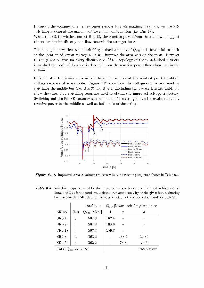
However, the voltages at all three buses recover to their maximum value when the SR-

switching is done at the extreme of the radial conguration (i.e. Bus 18).

When the SR is switched out at Bus 18, the reactive power from the cable will support

the weakest point directly and ow towards the stronger buses.

The example show that when switching a xed amount of QSR it is benecial to do it

at the location of lowest voltage as it will improve the area voltage the most. However

this may not be true for every disturbance. If the topology of the post-faulted network

is meshed the optimal location is dependent on the reactive power ow elsewhere in the

system.

It is not strictly necessary to switch the shunt reactors at the weakest point to obtain

voltage recovery at every node. Figure 6.17 show how the voltage can be recovered by

switching the middle bus (i.e. Bus 3) and Bus 4. Excluding the weaker Bus 18. Table 6.6

show the three-step switching sequence used to obtain the improved voltage trajectory.

Switching out the full SR capacity at the middle of the string allows the cables to supply

reactive power to the middle as well as both ends of the string.

5 10 15 20 25 30

Time, t [s]

0.65

0.7

0.75

0.8

0.85

0.9

0.95

1

1.05

Are

a A

bu

s v

olta

ge

s in

p.u

.

Bus 3, SR sw.

Bus 4, SR sw.

Bus 18, SR sw.

Bus 3, no sw.

Bus 4, no sw.

Bus 18, no sw.

1

23

Figure 6.17. Improved Area A voltage trajectory by the switching sequence shown in Table 6.6.

Table 6.6. Switching sequence used for the improved voltage trajectory displayed in Figure 6.17.

Total bus QSR is the total available shunt reactor capacity at the given bus, deducting

the disconnected SRs due to line outage. Qsw is the switched amount for each SR.

Total bus Qsw [Mvar] switching sequence

SR no. Bus QSR [Mvar] 1 2 3

SR3-4 3 507.8 162.4 - -

SR3-2 3 507.8 188.6 - -

SR3-18 3 507.8 156.8 - -

SR4-3 4 362.2 - 138.4 24.36

SR4-5 4 362.2 - 73.8 24.6

Total Qsw switched 768.6 Mvar

119

6.4.5 Large-disturbance Case 5: Dynamic load increase and

disconnection of lines in Area A.

This study case focuses on Area A with reference to Figure 6.1. The events of the

disturbance are:

Load ramp increase of 50 % in the area over a duration of 10 s starting from t = 0.1 s.

Permanent disconnection of Line 2-3 and shunt reactors, t = 5 s.

Permanent disconnection of Line 17-18 and shunt reactors, t = 5 s.

An attempt is made to plan an approach to calculate the amount of Qsw at certain buses

to minimize the voltage deviation between them. The post-disturbance Area A topology

is presented in Figure 6.18. Buses 18, 3 and 4 are now connected similar to a radial line

network. Under this condition it is possible to approximate the necessary Qsw at Buses 3

and 18 to obtain a very small deviation across the whole area.

5

14

34 18

Area A

Figure 6.18. Simplied post-disturbance topology of Area A

Referring to the voltage drop equation derived for two terminals connected through a

transmission line in (1.11), a simplied version is repeated here for convenience assuming

that the imaginary part is negligible and excluded. PR and QR represent the receiving

end active and reactive power while X and R represents the line series resistance and

impedance.

∆V =

(PRVR

)R+

(QRVR

)X (6.1)

Based on the equation, there is a component that is caused by active power and the

other by reactive power. Assuming that ∆V = 0, equation (6.2) is obtained which gives

a relationship between active and reactive power at the receiving end necessary to have

zero voltage deviation. The reactive power would have to ow in the opposite direction

of the active power to counter balance each other. The knowledge of the RX ratio of the

corresponding transmission line is also needed for this approach.

QR = −(R

X

)PR (6.2)

Applying this approach to the post-disturbance network of Area A, as shown in Figure

6.18, the amount of Qsw at Buses 3 and 18 can be approximated using (6.2), as the total

load demands at the buses are known. The new power ow of the network with this

approach is illustrated in Figure 6.19. It should be noted that the voltage dependency

of the power demand is unaccounted for. Qbal is the new reactive power ow in counter

direction to balance the drop due to active power. The RX ratios of Line 3-18 and Line 3-4

are 0.0708 and 0.0524 respectively.

120

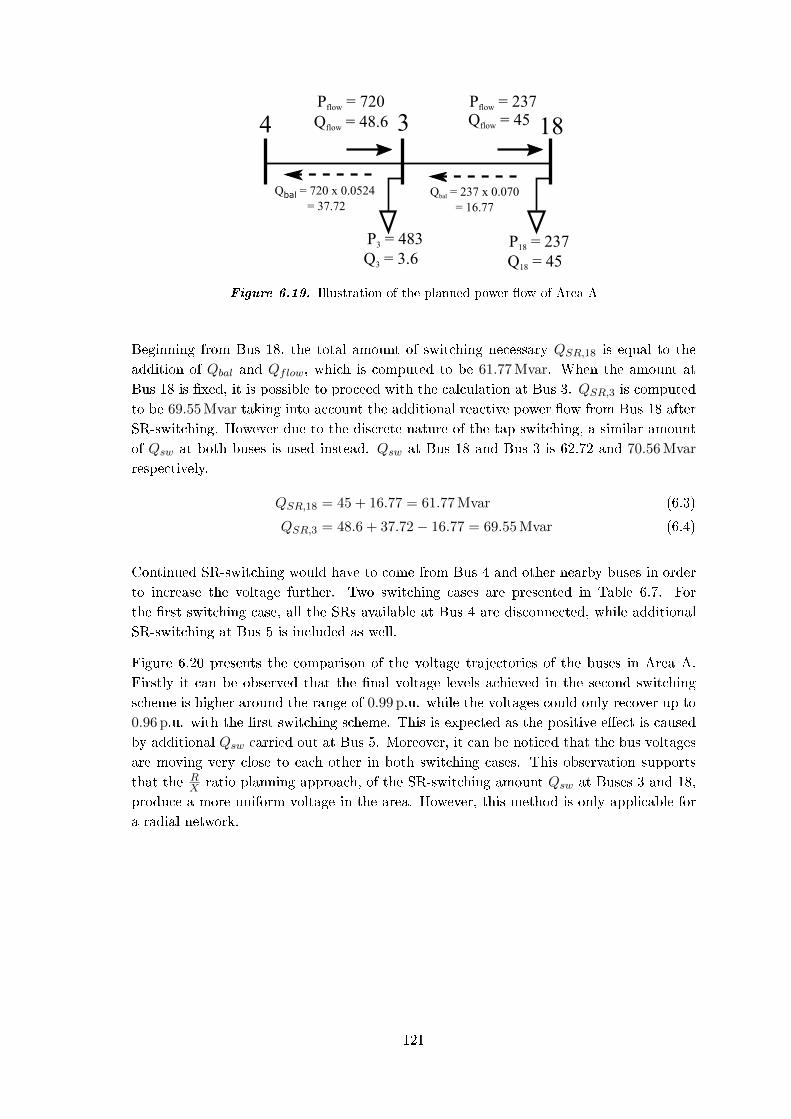
34 18Pflow = 720

Qflow = 48.6

Pflow = 237Qflow = 45

Q18 = 45

P18 = 237Q3 = 3.6

P3 = 483

Qbal = 720 x 0.0524

= 37.72

Qbal = 237 x 0.070

= 16.77

Figure 6.19. Illustration of the planned power ow of Area A

Beginning from Bus 18, the total amount of switching necessary QSR,18 is equal to the

addition of Qbal and Qflow, which is computed to be 61.77 Mvar. When the amount at

Bus 18 is xed, it is possible to proceed with the calculation at Bus 3. QSR,3 is computed

to be 69.55 Mvar taking into account the additional reactive power ow from Bus 18 after

SR-switching. However due to the discrete nature of the tap switching, a similar amount

of Qsw at both buses is used instead. Qsw at Bus 18 and Bus 3 is 62.72 and 70.56 Mvar

respectively.

QSR,18 = 45 + 16.77 = 61.77 Mvar (6.3)

QSR,3 = 48.6 + 37.72− 16.77 = 69.55 Mvar (6.4)

Continued SR-switching would have to come from Bus 4 and other nearby buses in order

to increase the voltage further. Two switching cases are presented in Table 6.7. For

the rst switching case, all the SRs available at Bus 4 are disconnected, while additional

SR-switching at Bus 5 is included as well.

Figure 6.20 presents the comparison of the voltage trajectories of the buses in Area A.

Firstly it can be observed that the nal voltage levels achieved in the second switching

scheme is higher around the range of 0.99 p.u. while the voltages could only recover up to

0.96 p.u. with the rst switching scheme. This is expected as the positive eect is caused

by additional Qsw carried out at Bus 5. Moreover, it can be noticed that the bus voltages

are moving very close to each other in both switching cases. This observation supports

that the RX ratio planning approach, of the SR-switching amount Qsw at Buses 3 and 18,

produce a more uniform voltage in the area. However, this method is only applicable for

a radial network.

121

Table 6.7. Two dierent switching cases in Area A for large Disturbance Case 5. The second

scheme includes all the events in the rst and only the extra events are shown.

Balance SR switching 1 Switching sequence

SR no. Bus QSR [Mvar] 1 2

SR4-5 4 98.4 100 % -

SR4-14 4 101.4 100 % -

SR4-3 4 162.4 100 % -

SR18-3 18 156.8 - 40 %

SR3-18 3 156.8 - 45 %

Total QSW 495.48 Mvar

Balance SR switching 2

SR5-4 5 98.4 100 % -

SR5-8 5 108.2 100 % -

Total QSW 702.08 Mvar

5 10 15 20 25 30

Time, t [s]

0.85

0.9

0.95

1

1.05

Are

a A

bus

vol

tage

s in

p.u

.

No SR sw.Balance SR sw. 1Balance SR sw. 2

Figure 6.20. Voltage trajectories of the buses in Area A for large-disturbance Case 5. Solid line:

Bus 3. Dotted-line: Bus 4. Dashed-line: Bus 18.

6.4.6 Large-disturbance Case 6: Loss of generation and transmission

line in Area F

The disturbances in this study case are imposed on Area F with reference to Figure

6.1. The study case is carried out for 25 % increased steady-state loading, such that

P = 1.25Pn at all load buses in the system. The power factor is kept constant. The

events of the disturbance are:

Three-phase fault at the terminal bus of SG9, t = 1 s.

Permanent disconnection of SG9 and transformer, t = 1.060 s.

Permanent disconnection of Line 26-29 and shunt reactors due to overloading, t = 2 s.

Permanent disconnection of Line 25-26 and shunt reactors due to overloading, t = 3 s.

122

The described disturbance lowers the voltages in Area F to a level between 0.7 p.u. and

0.8 p.u. However, the voltage is not only aected locally. Due to the loss of generation and

two transmission lines, the power ow of the network has been signicantly changed. As

power is no longer supplied locally in Area F, a larger amount of power must be supplied

from farther away. As a consequence the voltage in the opposite end of the network (Bus

8, 7, 6, 5 and 4) is lowered to just above 0.9 p.u.

Post-disturbance voltages at Bus 28 in Area F, Bus 27 neighbouring Area F, and distant

buses 4 and 8, are shown in Figure 6.21.

Due to the nature of the disturbance it is insucient to perform SR-switching in Area

F alone. Thus, the sequential SR-switching shown in Table 6.8 is performed. The result

of the SR-switching is likewise shown in Figure 6.21. Noting that improving the voltage

at distant buses by SR-switching has an increasing eect on the voltage in Area F as

well. Hence, the sequential method progressively switches Qsw starting from Area F

towards distant buses. The amount of Qsw is steadily reduced as the voltages at all buses

approaches 1 p.u.

0 2 4 6 8 10 12 14 16

Time, t [s]

0.6

0.7

0.8

0.9

1

Bu

s v

olta

ge

s in

p.u

.

Bus 28, SR sw.

Bus 27, SR sw.

Bus 8, SR sw.

Bus 4, SR sw.

Bus 28, no sw.

Bus 27, no sw.

Bus 8, no sw.

Bus 4, no sw.

1234 5 6

Figure 6.21. Comparison of voltage trajectories across the network with sequential SR-switching

and without SR-switching.

Table 6.8. Shunt reactor switching sequence in six steps involving shunt reactors in multiple

network areas.

Total bus Qsw [Mvar] switching sequence

SR no. Bus QSR [Mvar] 1 2 3 4 5 6

SR29-28 29 182.6 182.6 - - - - -

SR28-26 28 758.8 85.83 - - - - -

SR26-27 26 1878.7 - 70.28 - 26.36 - -

SR27-26 27 411.5 - 70.28 - 70.28 - -

SR4-3 4 362.2 - - 64.96 - 56.84 40.6

SR7-6 7 140.1 - - 33.16 - 29.02 20.73

SR8-9 8 444.30 - - 111.56 - 97.67 69.73

Total Qsw switched 1029.9 Mvar

123

If the sequence is performed faster, the voltage at all buses will recover faster. However,

a consequence of switching a high amount of SRs within a short time span is the risk of

over-voltages. Figure 6.22 show the result of switching the total Qsw = 1029.9 Mvar of

the sequence instantly in comparison to the progressive method. The voltages settle at

an equal equilibrium value, but the electromechanical transient is dierent. In the case

of instant switching, the high amount of reactive power supplied by the cables causes

the voltage to over-shoot before synchronous generators has time to adjust the excitation

level. Thus, ideally the SR-switching is performed in several small steps with a regulated

amount in each step.

0 2 4 6 8 10 12 14 16

Time, t [s]

0.6

0.7

0.8

0.9

1

1.1

1.2

Bus

vol

tage

s in

p.u

.

Bus 28, instant SR sw.Bus 27, instant SR sw.Bus 8, instant SR sw.Bus 4, instant SR sw.Bus 28, prog. SR sw.Bus 27, prog. SR sw.Bus 8, prog. SR sw.Bus 4, prog. SR sw.

3.5 4 4.5 50.8

1

1.2

Figure 6.22. Comparison of progressive sequential switching and instantaneous switching of an

equal amount: 1029.9 Mvar.

6.4.7 Combining shunt reactor switching with STATCOM

In continuation of the 9-bus analysis presented in Section 5.6.3, the combination of SR-

switching with dynamic voltage regulation is investigated in the 39-bus system. The

focus is on how dynamic switching of shunt reactors may replace the need for FACTS

devices, such as STATCOMs, by allowing cables to inject the necessary reactive current

in emergency situations. Hence, the question is if FACTS devices are necessary for large-

disturbance when shunt reactors are assumed controllable.

Based on the steady state V, P and Q,V analysis, and the voltage trajectory case studies,

it is decided to analyse the impact of placing two STATCOMs in the 39-bus system. Both

STATCOMs have a 50 Mvar rating. Two dierent combinations of STATCOM locations

are chosen:

Location 1, center of weak areas: The two STATCOMSs are placed at Bus 12

and Bus 28. Bus 12 is the weakest bus in Area G, while Bus 28 is the weakest bus

in Area F.

Location 2, area borders: The two STATCOMs are placed at the borders of the

weak areas of the network. Here Bus 5 and Bus 27 are chosen. Bus 5 is a connection

point of Area G and Area C (which proved to be a voltage sensitive area in the case

studies). Bus 27 is a connection point of Area F to the remaining network.

124

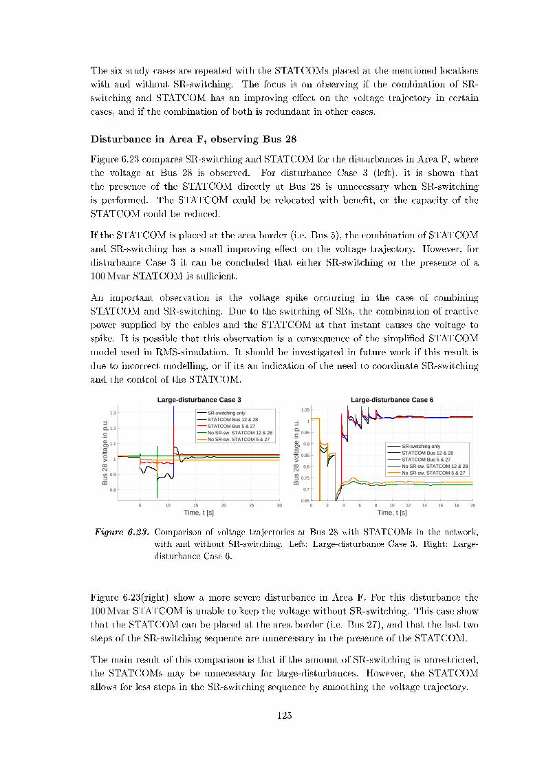
The six study cases are repeated with the STATCOMs placed at the mentioned locations

with and without SR-switching. The focus is on observing if the combination of SR-

switching and STATCOM has an improving eect on the voltage trajectory in certain

cases, and if the combination of both is redundant in other cases.

Disturbance in Area F, observing Bus 28

Figure 6.23 compares SR-switching and STATCOM for the disturbances in Area F, where

the voltage at Bus 28 is observed. For disturbance Case 3 (left), it is shown that

the presence of the STATCOM directly at Bus 28 is unnecessary when SR-switching

is performed. The STATCOM could be relocated with benet, or the capacity of the

STATCOM could be reduced.

If the STATCOM is placed at the area border (i.e. Bus 5), the combination of STATCOM

and SR-switching has a small improving eect on the voltage trajectory. However, for

disturbance Case 3 it can be concluded that either SR-switching or the presence of a

100 Mvar STATCOM is sucient.

An important observation is the voltage spike occurring in the case of combining

STATCOM and SR-switching. Due to the switching of SRs, the combination of reactive

power supplied by the cables and the STATCOM at that instant causes the voltage to

spike. It is possible that this observation is a consequence of the simplied STATCOM

model used in RMS-simulation. It should be investigated in future work if this result is

due to incorrect modelling, or if its an indication of the need to coordinate SR-switching

and the control of the STATCOM.

5 10 15 20 25 30

Time, t [s]

0.8

0.9

1

1.1

1.2

1.3

Bus

28

volta

ge in

p.u

.

Large-disturbance Case 3

SR-switching onlySTATCOM Bus 12 & 28STATCOM Bus 5 & 27No SR-sw. STATCOM 12 & 28No SR-sw. STATCOM 5 & 27

0 2 4 6 8 10 12 14 16 18 20

Time, t [s]

0.65

0.7

0.75

0.8

0.85

0.9

0.95

1

1.05

Bus

28

volta

ge in

p.u

.

Large-disturbance Case 6

SR-switching onlySTATCOM Bus 12 & 28STATCOM Bus 5 & 27No SR-sw. STATCOM 12 & 28No SR-sw. STATCOM 5 & 27

Figure 6.23. Comparison of voltage trajectories at Bus 28 with STATCOMs in the network,

with and without SR-switching. Left: Large-disturbance Case 3. Right: Large-

disturbance Case 6.

Figure 6.23(right) show a more severe disturbance in Area F. For this disturbance the

100 Mvar STATCOM is unable to keep the voltage without SR-switching. This case show

that the STATCOM can be placed at the area border (i.e. Bus 27), and that the last two

steps of the SR-switching sequence are unnecessary in the presence of the STATCOM.

The main result of this comparison is that if the amount of SR-switching is unrestricted,

the STATCOMs may be unnecessary for large-disturbances. However, the STATCOM

allows for less steps in the SR-switching sequence by smoothing the voltage trajectory.

125

Locating STATCOMs directly in weak areas is unnecessary in the tested cases, as shunt

reactors can be switched to let the cables supply the critical reactive power locally.

Similar analysis of SR-switching and STATCOMs performed for Area G and Area A is

located in Appendix H

6.5 Summary of voltage stability analysis in the IEEE

39-bus system

This section presents an overview of the large-disturbance voltage stability study carried

out in the IEEE 39-bus system. Since the investigation is done in a similar manner to the

9-bus study repetitive conclusions are not elaborated. Instead, the following provides the

additional conclusions of the 39-bus voltage stability analysis.

Conclusions on the voltage stability comparison of OHL systems and equivalent cable

systems:

V, P -characteristics show that the tendency observed in the 9-bus system is

conrmed in the 39-bus system.

Q,V - characteristics show that the cable-based system has higher slope (i.e. ∂Q/∂V )

in the voltage range of 1.0 p.u. at nominal loading levels. This indicates that

its voltage is less sensitive to the variation of reactive power at the bus. The

Q,V -characteristics of the investigated areas are also consistent with the area

characterization according to short-circuit calculations.

Conclusions on the guidelines for SR-switching. SR-switching is shown to help voltage

recovery. Considerations should be taken with focus on the following three elements:

1. Timing: Instants at which SR-switching is initiated

Progressive SR-switching is able to limit the voltage over-shoot and reduce the

risk of over-voltages. A smoother voltage characteristic could be achieved by

this method. Smooth voltage trajectories may be achieved by switching shunt reactors in

multiple steps.

2. Location: Location of switching with respect to disturbed area

SR-switching at any bus in an area improve the voltage levels of all buses in the

area. Switching at the bus displaying the lowest voltage is a good strategy, but

may not be optimal for every case. If the system is highly meshed, injecting

reactive current in other nodes may be more benecial for the overall power

ow. Distributing the same amount of SR-switching among multiple buses would

reduce voltage deviations between buses and thus produce a much more uniform

voltage characteristic in the area.

126

3. Amount: The amount necessary to achieve voltage improvement in an area.

Larger amount of SR-switching would result in a higher post-disturbance

voltage. Dependent on the availability of the area, areas with low capacitance due to

short lines may have insucient amount of SR capacity for voltage recovery.

In this case SR-switching may be performed in neighbouring areas. Planning of amount at certain buses to minimize voltage deviations between

buses in the area could be done by utilizing R/X ratio of the cables. This

approach is more easily applicable in radial type of network. It is likely that ∂Q/∂V -sensitivities can be utilized to design SR-switching. Due

to time constraints of the project presented in this thesis, a study of ∆Q/∆V -

based planning of SR-switching is not realised. This should be investigated in

future work. A brief discussion of linearised ∆Q/∆V slopes and their possible

use for SR-switching is located in Appendix I.

Conclusions on combining STATCOM with SR-switching:

SR-switching may remove the necessity for FACTS such as STATCOM when

assuming similar controllability.

If located in the disturbed area, the MVA rating of the STATCOMs may be reduced

if combined with SR-switching.

STATCOMs can be used to ne tune the voltage trajectory by smoothing the voltage.

Therefore the amount of SR-switching steps in a sequence may be reduced. To

provide this ability, STATCOMs do not need to be located in the disturbed area but

instead can be located at the borders between areas.

Additional conclusions: Short-circuit test is not an explicit indicator of network strength

for voltage stability

Area C recorded large voltage drops during RMS simulations conducted in study

cases contrary to the short-circuit results which indicates that it is a stronger area.

The observed contradiction is assumed due to its close proximity to SG1 that mainly

contributes short-circuit power to the area. On the other hand, SG1 is modelled with

no AVR included and therefore the dynamic regulation in that area is greatly reduced

in RMS simulation.

127

Discussion of results 7In this chapter the main results presented in this thesis are discussed. The focus is on

the limitations of the methodology, and comparison with published research on the topic:

stability of cable based HVAC power systems.

7.1 Comparison of results with published research

The authors of [19] compare CCT values of an OHL based SMIB system and a mixed cable-

OHL SMIB system. It is concluded that if the cable transmission line is compensated,

the CCT dierence of the OHL and the mixed line system is insignicant. Furthermore,

it is concluded that if the cable stretch of the mixed line is short (approximately 20 km),

the CCT values are equal even without compensation by SRs. The deviation between

the OHL system and the mixed-line system increases as the length of the cable stretch is

increased, unless corresponding compensation is introduced.

In this thesis CCT values of a SMIB system are compared for the OHL case and equivalent

cable case with and without SRs and SR-switching. Here it is found, that if the cable

system is uncompensated the CCT values are signicantly lower. However, it is important

to note that the system is a pure cable system, as opposed to the mixed line system, and

that the length of the lines is 100 km. In [19] the uncompensated generated reactive

power of the short cable stretch acts as compensation for the inductive OHLs in the

system. Hence, the results presented in this thesis conrms that increasing the length of

uncompensated cables lowers the CCT of the system, while introducing compensation in

the form of SRs equalizes the performance between OHL and cable systems. As presented

in Chapter 4, the dierence in CCT between the OHL base system and equivalent cable

system is approximately 6 % in the case of 100 % compensation. For large power systems,

such as the 39-bus system, it is found that the power ow cannot be solved unless cables

are compensated.

The authors of [19] nd that over-compensation of cable stretches longer than 20 km has an

improving eect on CCT, however no explanation as to why is given. A similar tendency

is observed in the transient 9-bus and 39-bus analysis in this thesis. The reason why is

presumably due to steeper P, δ-curves when SGs are operating in over-excitation mode,

resulting in reduced power-swing oscillations following large-disturbances. However, this

assumption should be conrmed in future work.

It is very important to note that the steady-state voltage stability analysis in the form

of V, P -curves yields the opposite result. In Chapter 5 and Chapter 6 it is shown that

under-compensating the cable system yields a higher load-ability with respect to voltage

stability margins. The author of [2] shows that the load-ability is higher for capacitive

networks, which conrms the tendency observed in V, P -curves for under-compensated

cables.

129

This contradicts the dynamic CCT analysis, which shows that over-compensation is

benecial. Thus, when analysing the inuence of changing compensation degree, one

should be aware of this when choosing stability index and methodology.

In reality the eect of increasing or decreasing the compensation degree should be a

relationship between improving the operation state of synchronous machines with respect

to P, δ and excitation level, and the balance of reactive power and voltage control in

the network. Naturally, the compensation degree cannot be increased indenitely while

observing an improved CCT. At a certain limit the arising problem of voltage instability

will dominate the system performance, and the CCT must necessarily drop in case of

further increment of the compensation degree. In other words, it can not be concluded

whether over- or under-compensation is better, as it is dependent on the parameters on

which the analysis is based and the operating condition of the system.

The authors of [19] do not discus switching of SRs for improving CCT. In this thesis it is

found that in a SMIB system, switching of SRs in an electromechanical transient following

a fault may improve CCT. Furthermore, it is found that SRs of disconnected lines should

be disconnected concurrently for improved CCT.

In [21] the authors nd that transmission cables should be suciently compensated to

avoid under-excitation of synchronous machines and to avoid over-voltages. Furthermore

is is found that SRs should be switched together with lines to avoid voltage steps exceeding

±3 %, while it is argued that it is benecial to reconnect SRs before reconnecting a cable

line. In this thesis the order of disconnecting and reconnecting lines and their SRs is not

investigated. However, it can be conrmed that it is necessary to disconnect SRs of long

cables that are taken out of service.

The authors of [22] propose a method to calculate the cable length required to compensate

inductive OHLs in mixed-line congurations. This is not investigated in this thesis, as the

entire OHL base system is replaced by an equivalent cable system. However, it is found

that under-compensation of cables improve V, P -load-ability, by allowing reactive power

to be supplied nearer inductive loads and compensation of line inductance. This eect is

similar to nding an optimal under-compensation degree (or cable length), which matches

the reactive power demand locally in the network.

In agreement, the authors of [41] and [42] conclude that under-compensation may be

benecial in the case of short cable lines. It is argued how SRs with tap changing ability

can be used to regulate the voltage, by letting the cables supply reactive power. However

the analysis is performed for steady-state analysis and load-ability, and is not extended

to large-disturbance.

The authors of [32] seek to optimize the location and size of dynamic reactive power

compensation. The method presented is based on identifying the network node displaying

the weakest voltage trajectories for various disturbances. The authors argue how

compensating the weakest point entail the largest overall voltage improvement of the

network by indirect improvement the neighbouring nodes. Although intuitive, this eect

is conrmed in the study of SR-switching presented in this thesis, where immediate

compensation in the area of lowest voltage is most eective for the tested cases.

130

The work done in [32] focuses on FACTS devices. However, a similar method could be

adopted in future work in regards to fast tap-changing and switching of SRs.

In this thesis the voltage stability is assessed by comparing voltage trajectories against an

under-voltage limit and by steady state analysis of V, P and Q,V -characteristics. An issue

of this methodology is that the actual stability margins, of the various study cases and line

parameters, are undened for large-disturbances. In other words, the methods used do

not provide a comparable index which provides information about the so called distance

to instability. The authors of [34] compare several stability indices based on analysing the

power ow Jacobian and eigenvalues, and propose a new improved index. The proposed

method is designed for large-disturbance and utilizes dV/dQ to identify nodes where the

voltage is most sensitive to injection of reactive power (i.e. weak point) combined with

time domain solutions to include electromechanical dynamics of generation and loads.

Adopting the method proposed in [34], may be advantageous in future work of the topic

presented in this thesis. With a well dened stability index the eects of SR-switching

may be more systematically assessed and compared.

7.2 Discussion of methodology and validity of results

Modelling reections:

1. The dynamic models of electrical machinery, excitations systems and governors

are not developed specically for this thesis. Instead, standard models from

the DIgSILENT library and the included 9-bus and 39-bus systems are used.

Alternatively the analysis could be based on a model of a real modern power

system. In [21] the analysis is carried out using a model of the Dutch power system.

The benet of using the model of a real modern power system is up-to-date and

representative model parameters of generation, transmission and loads.

2. Several dynamic power system components are not included in the models. The list

includes transformer OLTC, under- and over-voltage protection, OEL and UEL, and

dynamic load models such as induction machines. Especially, the voltage stability

results may be aected by the lack of these models, as their presence is expected

to alter the cascading voltage instability events. In this thesis voltage instability

is assumed when the bus voltages does not satisfy an under-voltage limit following

the given disturbance. However, an actual collapse of the system voltages is not

observed.

3. In this thesis the simulations were performed for up to 30-40 seconds at the most. If

slow dynamics such as OLTC and OEL/UEL are included in the models, the time

frame should be included to capture a cascading event.

4. The innite bus of the SMIB system is not modelled in the classical way, with an

ideal voltage source behind a reactance. Thus, the voltage at the end bus is not

kept at 1 p.u. as the external grid used has a nite short-circuit power. This should

be kept in mind when comparing the results presented in this thesis to other SMIB

studies.

131

5. The transmission lines are π-modelled such that the capacitance is lumped to the line

ends. Thus, the reactive power generated by cable capacitance is supplied directly

at the ends, where the shunt reactors are located. In reality the capacitance is

distributed, and the reactive current ows through line inductance towards the end

points. Lumped modelling is briey discussed in Section 3.3.2. It may be relevant

to test if there is a notable dierence in the stability tendencies for SR-switching

whether capacitance is distributed or lumped in future work.

6. The CCT analysis is performed without reactive power capability limits of the

synchronous generators. The power ow (i.e. initial conditions of the RMS-

simulation) is aected by the capability limits, which would reect on the studies of

over- and under-compensation of cables.

7. The CCT calculations are performed using a power-angle limit of δ = 179 . Another

limit can be argued for and chosen, which will aect the CCT values. However, the

tendencies should remain.

8. In the transient stability analysis (i.e. power angle and CCT), the composite

polynomial model is not used. In the 9-bus system all loads are modelled as constant

Z, while in the 39-bus the loads are modelled as constant current I for P , and

constant Z for Q. These are the basic settings in the system. Changing to the

composite model presented in voltage stability analysis is expected to lower the

obtained CCT values.

Assumptions for equivalent cable system and shunt-reactors:

1. The shunt reactors are dimensioned to compensate 100 % of the reactive power

generated by the cable capacitance. This is done without considering any deviation

in system voltages between the OHL case and cable case after compensation. In [21],

compensation is designed such that the bus voltages does not deviate by more than 2

% between the cable case and the OHL case. Furthermore the reactive power output

of SGs does not deviate more than 1 % between the OHL case and cable case. Table

F.6 and Table F.7 in Appendix F compare the reactive power output of SGs Qo and

the load bus voltages between the 39-bus system base case and the equivalent cable

system. The majority of the load buses satisfy the maximum 2 % deviation criterion

given in [21]. Three buses violate the criterion, but with a maximum deviation of

2.68 %. However, the Qo deviations are signicantly larger. In the worst case the

reactive power output is increased by 400 %. Generally the reactive power output

of most SGs is increased by 14 % to 56 % in the cable case. A reason may be the

fact that the capacitance of the OHL base case is uncompensated and thus the lines

are generating reactive power. A more signicant impact are observed for the longer

lines.

2. When replacing the OHL base system with the equivalent cable system it is assumed

that one OHL is replaceable by one equivalent cable. However, due to dierences

in ampacity between cables and OHLs it may be necessary to have more cables

in parallel in the equivalent case. The guidelines in [37] used for the creating the

equivalent case do not compare the ampacity for the given OHL and cable. If more

cables needs to be put in parallel it will change the network impedance and aect

the results.

132

3. It is assumed that shunt reactors can be disconnected and reconnected instanta-

neously, and that all shunt reactors have the ability to tap change within few seconds.

According to [20] tap changing of commercial shunt reactors has a time delay of ap-

proximately 10 s. The feasibility of fast SR-switching and the technical challenges

should be investigated in future work.

7.3 Future work

Following the discussion of the results and methods of this project, this section lists an

overview of the future work that could be done for further studies and to provide a more

comprehensive analysis of the relevant topics.

Voltage stability index

An important issue that is lacking in the project is the ability to predict large-disturbance

voltage instability. This can be solved by utilizing a voltage sensitivity index that assesses

stability margins of the system. Possibly an index which is based on dV/dQ method may

be used as it gives indications on how much SR-switching is necessary to prevent a voltage

collapse.

Location of SR placement

Only one conguration of the SR distribution is considered in the project, which is 50 % at

each end of the cable. The analysis could be expanded to include more SR congurations

in the system for further comparison of stability tendencies and performance.

Optimisation of SR switching

Several properties have been considered with regards to SR-switching in order to improve

the overall performance of the system following a disturbance. However a general approach

to the planning of switching as a function of voltage magnitude and time is not established.

Therefore an optimised SR-switching strategy based on bus voltage magnitude and dV/dQ

sensitivity could be explored.

Dynamic SR modelling

SR-switching is performed manually in the project by utilizing a tap event. An automated

alternative could be used by implementing dynamic modelling of each SR element in

DIgSILENT PowerFactory. This could be done by developing a DSL model with measured

voltage as the input signal. Appropriate time delays and droop controls could be included

in the modelling. This way sensitivity studies could be performed of the permissible SR-

switching time delay and the size of discrete tap steps. Hence the SR-switching would be

more comparable with FACTS devices.

Feasibility study of SR switching

In this project SR tap-switching is assumed to be fast acting without any restrictions

on the amount of switching. This assumption is in contrast to a typical behaviour of

tap-changer with long delays and limited tap-position per movement due to mechanical

limitations. There may also be other implications due to fast action detrimental to the

system that need to be considered.

133

Nonetheless results indicate that fast SR switching would improve the voltage stability

performance of the system signicantly therefore its feasibility and potential is worth

investigating. An instant switching SR has essentially the same behaviour as FACTS

devices.

Over-compensation on CCT improvement

Transient analysis show that over-compensation of cable system has an improving transient

stability tendency and presumably explained by the steeper P, δ-curves which is a result

of increasing over-excitation level of SGs. This explanation should be questioned with the

purpose of conrming or disproving.

π modelling

All the transmission lines are modelled as π-models with lumped parameters. Distributed

parameters could be used to emulate a more realistic representation of cables, especially

when big voltage variations between the terminals are observed. As such the reactive power

ow would be inuenced signicantly. Hence, it should be investigated if distribution of

line parameters of long HVAC cables inuence the assessed stability margins signicantly

compared to lumped modelling.

Realistic power system model

The stability analysis could be done on a more modern and comprehensive power system

model, for example by modelling a part of the Danish transmission network. By modelling

a modern power system, the inuence of many existing components such as HVDC, wind

turbines and PV generators would be included. Such components are typically absent

in conventional standard models such as the IEEE 9-bus and 39-bus systems. Another

advantage of investigating a realistic system is that the actual stability margins (such as

CCT) obtained may represent the expected behaviour of the real system.

STATCOM modelling

Emphasis should be placed on valid modelling of the STATCOM. Thus making the

comparison between SR-switching and STATCOM performance more conclusive.

134

Conclusion 8The goal of this thesis is to investigate how undergrounding of long HVAC transmission

lines aect the stability limits of multi-machine power systems. This is accomplished by

simulating large-disturbance electromechanical transients in DIgSILENT PowerFactory.

The stability is assessed for generic power systems by the classical denitions of transient

stability and voltage stability. The analysis is initiated on a simple single-machine innite

bus system, and is expanded to the IEEE 9-bus and 39-bus multi-machine power systems.

The stability performance of the OHL base case system is compared against an equivalent

cable system. The main ndings of the thesis are hereby presented.

Theoretical sensitivity studies of transmission line L and C are performed in a SMIB

system. The theoretical observations are indicative for the comparison of OHL and

equivalent cable lines including compensation. In reality the line parameters are

determined by the transmission line design, and is not simply changed. The tendencies

show that increasing either L or C has a transiently destabilizing eect, expressed by

decreasing CCT, when the SG is initially operated at unity power factor. Increasing series

parameters may improve the faulted P, δ-state due to increased fault loop impedance,

similarly to increasing the fault distance. However, topological dierences between pre-

and post-faulted systems give rise to larger power angle oscillations as line parameters

are increased. Being a pi-modelled shunt parameter, the inuence of C is insensitive to

fault location as opposed to L. Increasing C may reduce CCT by signicantly increasing

the steady-state power angle due to under-excitation of the synchronous generator.

Compensation of the reactive power generated by the capacitance reduces the power angle

and the CCT is improved.

Comparison of the transient stability performance in both SMIB and multi-machine

systems show that the equivalent cable system with 100 % compensation has consistently

longer CCT than the OHL base system, provided that the corresponding SRs of the

faulted line are disconnected when the line is taken out of service. In some cases the CCT

of the cable case is longer, even without switching of shunt reactors. This is a natural

consequence of lower L due to the geometrical dierences of OHL and equivalent cables.

Increasing the SR compensation degree has an improving eect on the CCT. This is

tested up to 115 %, and is a conrmation of the ndings in [19]. Inductive behaviour of

the network requires increased excitation level of synchronous machines, which results

in a steeper P, δ-curve and smaller power angle oscillations. However, this result is

not explicitly conclusive for every aspect power system stability. In contradiction the

voltage stability analysis show that under-compensation of cables improve the V, P load-

ability of the network. Being under-compensated, the cables supply reactive power to line

inductance, inductive loads and transformers locally.

135

Hence the optimal compensation degree must necessarily be a balance of both synchronous

generator excitation level and the ability to supply reactive power locally in the network.

The V, P -characteristics in both 9-bus system and 39-bus system show that the 100 %

compensated equivalent cable system display higher steady state load-ability than the

OHL base system. Furthermore, the stability margin of the cable system is signicantly

larger, even when the SR compensation is increased by 25 %. Similarly Q,V -curves of

the equivalent cable systems prove to be slightly steeper. Hence a high ∂Q/∂V indicating

lower voltage sensitivity to changes in reactive power ow.

Dynamically the voltage stability is assessed through case studies of voltage trajectory

analysis. The bus voltages following large-disturbances are evaluated against an under-

voltage limit. An advantage of the cable based system is the presence of SRs. The cable

based system is equipped with a signicant amount of local reactive power support, by

assuming that SRs can be tap changed and switched in and out of service as fast as

necessary. By decreasing the shunt reactance during an electromechanical transient, the

large amount of capacitive current generated by the cables is injected into the network

inductance and thereby imposing a voltage.

It is shown for various cases that SR-switching can improve voltage trajectories to satisfy

the under-voltage limit. This ability is unavailable in the OHL base system, where

compensation for steady state operation is unnecessary. However, the real question is how

to generalize the planning of SR-switching for large-disturbance events. Three dierent

properties of SR-switching are investigated through case studies: Amount, location and

timing.

It is concluded that the SR-switching should be performed progressively to reduce the

risk of transient over-voltages. A smooth voltage recovery can be achieved by sequentially

switching the buses measuring the lowest voltages. The overall system improvement should

be considered and not limited to the lowest voltage nodes. Distributing the amount of SR-

switching among multiple buses and areas reduce voltage deviations and produce a more

uniform voltage characteristic. The amount of SR-switching necessary should be based

on the magnitude of the post-disturbed voltage. However, the results of SR-switching

presented in this thesis only bring indications towards improving the voltage trajectory.

Further work is required in order to generalize and quantify the properties of SR-switching.

Lastly it is shown how SR-switching may reduce the need of dynamic voltage regulation in

the form of FACTS. By performing SR-switching the necessary capacity of STATCOMS

may be signicantly reduced or completely substituted.

136

Bibliography

[1] First report of power system stability, AIEE Subcommittee on Interconnections

and Stability Factors, pp. 51 80, 1926.

[2] P. Kundur, Power System Stability and Control. McGraw-Hill, 1994.

[3] P. Kundur, J. Paserba, V. Ajjarapu, G. Andersson, A. Bose, C. Canizares,

N. Hatziargyriou, D. Hill, A. Stankovic, C. Taylor, T. V. Cutsem, and V. Vittal,

Denition and classication of power system stability, IEEE Transactions on

Power Systems, vol. 19, pp. 1387 1401, may 2004.

[4] Final report on the august 14, 2003 blackout in the united states and canada:

Causes and recommendations, U.S.-Canada Power System Outage Task Force, apr

2004.

[5] REN21, Renewables 2015 global status report, pp. 3032, 2015. [Online].

Available: http://www.ren21.net/wp-content/uploads/2015/07/REN12-GSR2015_

Onlinebook_low1.pdf

[6] D. Gautam, V. Vittal, and T. Harbour, Impact of Increased Penetration of

DFIG-Based Wind Turbine Generators on Transient and Small Signal Stability of

Power Systems, IEEE Transactions on Power Systems, vol. 24, pp. 1426 1434,

aug 2009.

[7] ing.dk, Et blaesende 2015 gav rekord i vindkraft, Ingenioeren, January 2016.

[Online]. Available:

http://ing.dk/artikel/et-blaesende-2015-gav-rekord-i-vindkraft-181552

[8] S. Eftekharnejad, V. Vittal, G. T. Heydt, B. Keel, and J. Loehr, Impact of

Increased Penetration of Photovoltaic Generationon Power Systems, IEEE

Transactions on Power Systems, vol. 28, pp. 893 901, may 2013.

[9] Energinet.dk, Cable to the Netherlands - COBRAcable, www.energinet.dk, jun

2015. [Online]. Available:

https://www.energinet.dk/EN/ANLAEG-OG-PROJEKTER/Anlaegsprojekter-el/

Kabel-til-Holland-COBRA/Sider/Kabel-til-Holland-COBRA.aspx

[10] Nationalgrid and Energinet.dk, Vikinglink, www.viking-link.com, feb 2016.

[Online]. Available: http://viking-link.com/the-project/

[11] Energinet.dk, Tennet and Energinet.dk to reinforce electricity connection across

the Danish-German border, www.energinet.dk, apr 2015. [Online]. Available:

http://energinet.dk/EN/ANLAEG-OG-PROJEKTER/Nyheder/Sider/

TenneT-og-Energinet-dk-vil-forstaerke-el-forbindelse-over-tysk-dansk-graense.aspx

[12] Energinet.dk, Kriegers Flak: Combined Grid Solution, www.energinet.dk, nov

2015. [Online]. Available:

137

http://energinet.dk/EN/ANLAEG-OG-PROJEKTER/Anlaegsprojekter-el/

Forbindelse-til-Tyskland-Kriegers-Flak-CGS/Sider/default.aspx

[13] L. Zhang, L. Harnefors, and H.-P. Nee, Interconnection of Two Very Weak AC

Systems by VSC-HVDC Links Using Power-Synchronization Control, IEEE

Transactions on Power Systems, vol. 26, pp. 344 355, feb 2011.

[14] Energinet.dk, Netudviklingsplan 2013, vol. Dok. 46329/13, Sag 10/7196, May

2013. [Online]. Available: http://www.energinet.dk/SiteCollectionDocuments/

Danske%20dokumenter/El/Netudviklingsplan%202013.PDF

[15] Energinet.dk, Kabelhandlingsplan 2013, vol. Dok. 21597/13, Sag 10/7196, May

2013. [Online]. Available: http://www.energinet.dk/SiteCollectionDocuments/

Danske%20dokumenter/El/Kabelhandlingsplan%202013.PDF

[16] Statistics of AC underground cables in power networks, CIGRE Technical

Brochure, vol. 338, dec 2007.

[17] General Guidelines for the Integration of a New Underground Cable System in the

Network, CIGRE Working Group B1.19, 2004.

[18] F. F. da Silva and C. L. Bak, Electromagnetic Transients in Power Cables.

Springer, 2013.

[19] M. G. Ippolito, F. Massaro, G. Morana, and R. Musca, Transient Stability

Assessment of SMIB System with Mixed Overhead-Cable Line - Sensitivity

Analysis, Universities Power Engineering Conference (UPEC), vol. 44, sep 2009.

[20] C.-J. Chou, C.-Y. Han, Y.-K. Wu, and C.-Y. Lee, Study on Voltage Stability of

Island Grid Supplied by Large Grid with Long Submarine Cables Considering

Dierent Load Patterns. Utility Exhibition on Power and Energy Systems: Issues

and Prospects for Asia (ICUE), sep 2011.

[21] H. Khalilnezhad, M. Popov, J. A. Bos, and K. P. J. Jansen, Inuence of partial

undergrounding on the transient stability of EHV power transmission systems,

Electric Power Systems Research, vol. 131, pp. 126 138, 2016.

[22] U. Karki, D. Gunasekaran, and F. Z. Peng, Reactive Compensation of Overhead

AC Transmission Lines using Underground Power Cables, Power and Energy

Society General Meeting, may 2015.

[23] P. W. Sauer and M. A. Pai, Power System Dynamics and Stability. Stipes

Publishing Co., 1997.

[24] M. W. Mustafa and M. R. Ahmad, Transient Stability Analysis of Power System

with Six-Phase Converted Transmission Line, in IEEE International Power and

Energy Conference, 2006 (PECON '06), Putrajaya, Malaysia, Nov. 2006, pp.

262266.

[25] P. M. Anderson and A. Fouad, Power System Control and Stability. IEEE Press,

1994.

138

[26] M. J. Basler and R. C. Schaefer, Understanding of power system stability, in Pulp

and Paper Industry Technical Conference, 2007. Conference Record of Annual,

Williamsburg, VA, June 2007, pp. 3747.

[27] F. Lu and J.-L. Yu, Using Critical Machine Couple Equal Area Criterion to Assess

Multi-Machine System Stability, in

Power and Energy Engineering Conference, 2009. APPEEC 2009. Asia-Pacic,

Wuhan, March 2009, pp. 14.

[28] N. Yorino, A. Priyadi, H. Kakui, and M. Takeshita, A New Method for Obtaining

Critical Clearing Time for Transient Stability, IEEE Transactions on Power

Systems, vol. 25, pp. 16201626, Aug 2010.

[29] A. Paul and N. Senroy, Critical clearing time estimation using synchrophasor

data-based equivalent dynamic model, IET Generation, Transmission and

Distrbution, vol. 9, pp. 609614, Apr 2015.

[30] L. G. W. Roberts, A. R. Champneys, K. R. W. Bell, and M. di Bernardo,

Analytical Approximations of Critical Clearing Time for Parametric Analysis of

Power System Transient Stability, IEEE Journal on Emerging and Selected Topics

in Circuits and Systems, vol. 5, pp. 465476, Sept 2015.

[31] D. K. Cheng, Field and Wave Electromagnetics. Pearson, 1989.

[32] R. Xia, Z. Hu, and Q. Zhou, Optimal Planning of Dynamic VAR Compensation

Based on Transient Voltage Stability Analysis, POWERCON, pp. 916921, Oct

2014.

[33] F. A. Althowibi and M. W. Mustafa, Voltage Stability Calculations in Power

Transmission Lines: Indications and Allocations, IEEE International Conference

on Power and Energy, pp. 390 394, dec 2010.

[34] S. Konar, D. Chatterjee, and S. Patra, V-Q sensitivity-based index for assessment

of dynamic voltage stability of power systems,

IET Generation, Transmission and Distribution, vol. 9, pp. 677685, 2015.

[35] N. Qin, V. Akhmatov, T. Lund, H. Abildgaard, and M. K. Jørgensen, Voltage

Stability Analysis of the Eastern Danish Power System with a High Share of Wind

Energy, 10th International Workshop on Large-Scale Integration of Wind Power

into Power Systems as well as on Transmission Networks for Oshore Wind Power

Plants, vol. 10, oct 2011.

[36] DIgSILENT, DIgSILENT PowerFactory Technical Reference Documentation:

Synchronous Machine, ElmSym, TypSym, www.digsilent.net, 2016. [Online].

Available: http://www.digsilent.de/index.php/downloads.html

[37] Cable Systems Electrical Characteristics, Working Group B1.30 CIGRE, apr 2013.

[38] DIgSILENT, DIgSILENT PowerFactory Technical Reference Documentation:

General Load, ElmLod, www.digsilent.net, 2016. [Online]. Available:

http://www.digsilent.de/index.php/downloads.html

139

[39] IEEE Guide for the Application of Protective Relays Used for Abnormal Frequency

Load Shedding and Restoration, IEEE, aug 2007.

[40] P. Kundur, K. Morison, and B. Gao, Practical considerations in voltage stability

assessment, IEEE Electrical Power and Energy Systems, vol. 15, pp. 205215, 1993.

[41] F. M. Gatta and S. Lauria, Very long EHV cables and mixed overhead-cable lines.

Steady-state operation, Power Tech, 2005.

[42] S. Lauria, F. M. Gatta, and L. Colla, Shunt compensation of EHV Cables and

Mixed Overhead-Cable Lines, Power Tech, pp. 13441349, 2007.

[43] IEEE Power Engineering Society, IEEE Recommended Practice for Excitation

System Models for Power System Stability Studies. 2005.

[44] F. M. Gonzalez-Longatt and J. L. Rueda,

PowerFactory Applications for Power System Analysis. Springer, 2014.

140

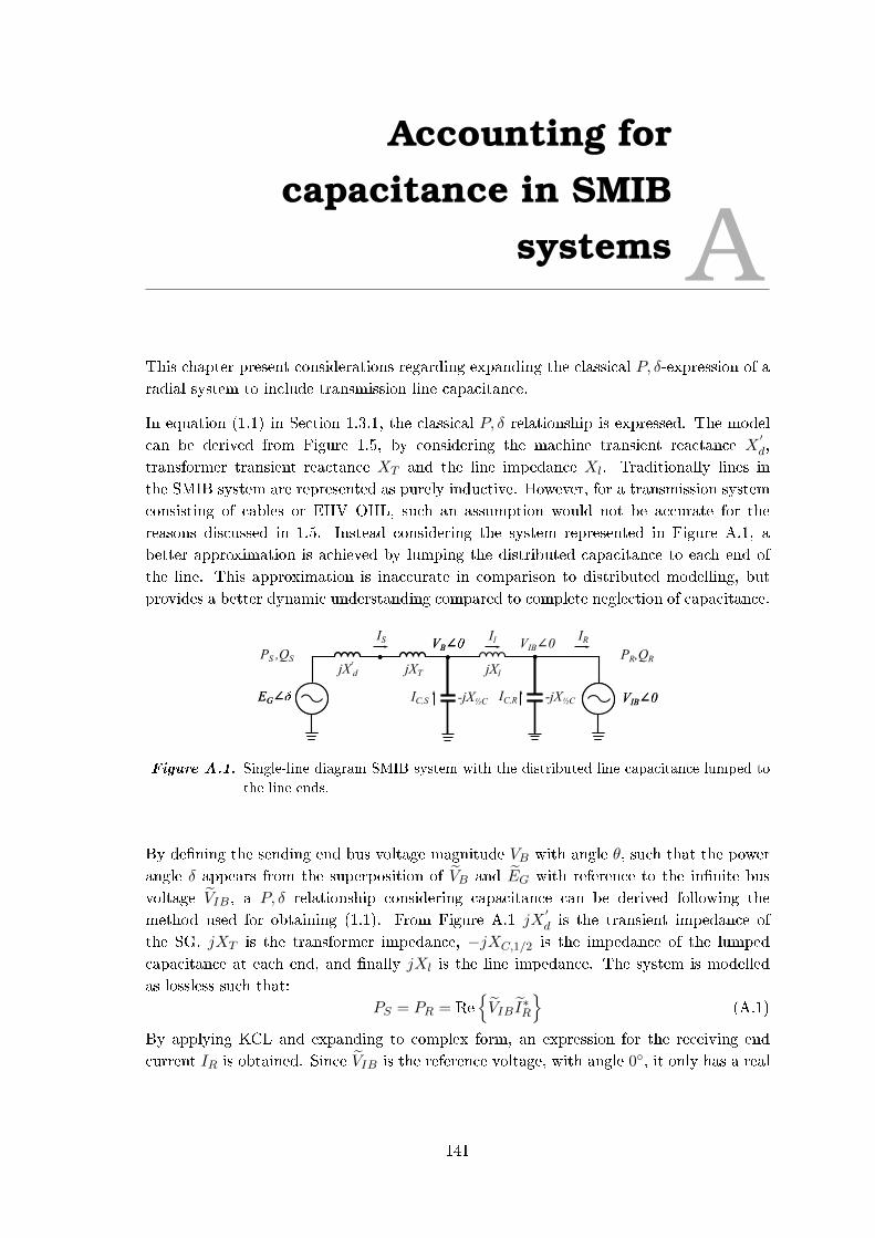
Accounting forcapacitance in SMIB

systems AThis chapter present considerations regarding expanding the classical P, δ-expression of a

radial system to include transmission line capacitance.

In equation (1.1) in Section 1.3.1, the classical P, δ relationship is expressed. The model

can be derived from Figure 1.5, by considering the machine transient reactance X′d,

transformer transient reactance XT and the line impedance Xl. Traditionally lines in

the SMIB system are represented as purely inductive. However, for a transmission system

consisting of cables or EHV OHL, such an assumption would not be accurate for the

reasons discussed in 1.5. Instead considering the system represented in Figure A.1, a

better approximation is achieved by lumping the distributed capacitance to each end of

the line. This approximation is inaccurate in comparison to distributed modelling, but

provides a better dynamic understanding compared to complete neglection of capacitance.

VB∠

VIB∠0EG∠

VB∠

VIB∠0EG∠

jX'd jXT jXl

-jX½C

IS

IC,S

Il

PS ,QS PR,QR

-jX½CIC,R

VIB∠0IR

Figure A.1. Single-line diagram SMIB system with the distributed line capacitance lumped to

the line ends.

By dening the sending end bus voltage magnitude VB with angle θ, such that the power

angle δ appears from the superposition of VB and EG with reference to the innite bus

voltage VIB, a P, δ relationship considering capacitance can be derived following the

method used for obtaining (1.1). From Figure A.1 jX′d is the transient impedance of

the SG, jXT is the transformer impedance, −jXC,1/2 is the impedance of the lumped

capacitance at each end, and nally jXl is the line impedance. The system is modelled

as lossless such that:

PS = PR = ReVIB I

∗R

(A.1)

By applying KCL and expanding to complex form, an expression for the receiving end

current IR is obtained. Since VIB is the reference voltage, with angle 0, it only has a real

141

component, such that VIB = VIB cos(0) + jVIB sin(0) = VIB.

IR = IS + IC,S + IC,R ⇒ (A.2)

IR =EG − VB

j(X′d +XT )

+0− VB−jXC,1/2

+0− VIB−jXC,1/2

⇒ (A.3)

IR =EG − VB

j(X′d +XT )

+VB

jXC,1/2+

VIBjXC,1/2

(A.4)

IR =(EG cos (δ) + jEG sin (δ))− (VB cos (θ) + jVB sin (θ))

j(X′d +XT )

+(VB cos (θ) + jVB sin (θ))

jXC,1/2+

VIBjXC,1/2

(A.5)

IR =−jEG cos(δ) + EG sin(δ) + jVB cos(θ)− VB sin(θ)

X′d +XT

+−jVB cos(θ) + VB sin(θ)

XC,1/2+−jVIBXC,1/2

(A.6)

PS = ReVIB IR

⇒ PS = VIBRe

I∗R

(A.7)

By complex conjugation and substitution of (A.6) into (A.7), the expression for P (δ) is

obtained in (A.8). The expression assumes the total capacitance is equally lumped at each

end, such that XC,1/2 = 12XC .

PS =VIBEG sin(δ)− VIBVB sin(θ)

X′d +XT

+2VIBVB sin(θ)

XC(A.8)

At a rst look it may seem odd that the expression in (A.8) is independent of the line

reactance Xl. However, the dependency of Xl appears indirectly from the sending end

bus voltage VB as expressed in (A.9).

VB = VIB − IR(jXl) (A.9)

The capacitance lumped at the receiving end of the line does not have an impact on

the P, δ-characteristic, as it is cancelled when taking the real part of the expression in

(A.6). This is a consequence of the model, assuming that the voltage at the receiving

end is constant VIB∠0, despite the presence of the capacitor. However, it is reasonable

that the capacitance lumped at the sending end bus, will have a greater impact on the

P, δ-characteristic of the local SG in a real system.

Expanding (A.8) yields (A.10), where the term highlighted by a box is the classical P (δ)

expression, with the exception of the inductive line reactance Xl. The model is still

dependent on the eld voltage EG and the power angle associated with the ow of active

and reactive power through X′d and XT . However, the two additional terms imply that the

presence of the capacitor at the sending end of the line changes the non-linear power-angle

relationship. The extra terms are independent of EG, and are primarily associated with the

voltage at the sending end of the line, VB∠θ. The bus voltage VB∠θ is dependent on the

142

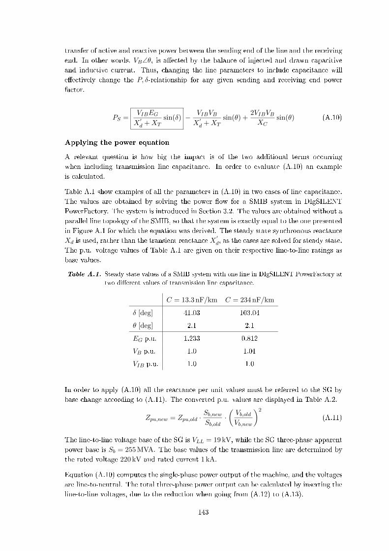
transfer of active and reactive power between the sending end of the line and the receiving

end. In other words, VB∠θ, is aected by the balance of injected and drawn capacitive

and inductive current. Thus, changing the line parameters to include capacitance will

eectively change the P, δ-relationship for any given sending and receiving end power

factor.

PS =VIBEG

X′d +XT

sin(δ) − VIBVB

X′d +XT

sin(θ) +2VIBVBXC

sin(θ) (A.10)

Applying the power equation

A relevant question is how big the impact is of the two additional terms occurring

when including transmission line capacitance. In order to evaluate (A.10) an example

is calculated.

Table A.1 show examples of all the parameters in (A.10) in two cases of line capacitance.

The values are obtained by solving the power ow for a SMIB system in DIgSILENT

PowerFactory. The system is introduced in Section 3.2. The values are obtained without a

parallel line topology of the SMIB, so that the system is exactly equal to the one presented

in Figure A.1 for which the equation was derived. The steady state synchronous reactance

Xd is used, rather than the transient reactance X′d, as the cases are solved for steady state.

The p.u. voltage values of Table A.1 are given on their respective line-to-line ratings as

base values.

Table A.1. Steady state values of a SMIB system with one line in DIgSILENT PowerFactory at

two dierent values of transmission line capacitance.

C = 13.3 nF/km C = 234 nF/km

δ [deg] 41.03 103.04

θ [deg] 2.1 2.1

EG p.u. 1.233 0.812

VB p.u. 1.0 1.01

VIB p.u. 1.0 1.0

In order to apply (A.10) all the reactance per unit values must be referred to the SG by

base change according to (A.11). The converted p.u. values are displayed in Table A.2.

Zpu,new = Zpu,old ·Sb,newSb,old

·(Vb,oldVb,new

)2

(A.11)

The line-to-line voltage base of the SG is VLL = 19 kV, while the SG three-phase apparent

power base is Sb = 255 MVA. The base values of the transmission line are determined by

the rated voltage 220 kV and rated current 1 kA.

Equation (A.10) computes the single-phase power output of the machine, and the voltages

are line-to-neutral. The total three-phase power output can be calculated by inserting the

line-to-line voltages, due to the reduction when going from (A.12) to (A.13).

143

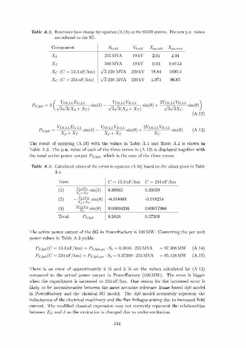
Table A.2. Reactance base change by equation (A.11) on the SMIB system. The new p.u. values

are referred to the SG.

Component Sb,old Vb,old Xpu,old Xpu,new

Xd 255 MVA 19 kV 2.01 2.01

XT 500 MVA 19 kV 0.03 0.0153

XC (C = 13.3 nF/km)√

3 220 MVA 220 kV 18.84 1690.4

XC (C = 234 nF/km)√

3 220 MVA 220 kV 1.071 96.05

PS,3ph = 3

(VIB,LLEG,LL√3√

3(Xd +XT )sin(δ)−

VIB,LLVB,LL√3√

3(Xd +XT )sin(θ) +

2VIB,LLVB,LL√3√

3XC

sin(θ)

)(A.12)

PS,3ph =VIB,LLEG,LLXd +XT

sin(δ)−VIB,LLVB,LLXd +XT

sin(θ) +2VIB,LLVB,LL

XCsin(θ) (A.13)

The result of applying (A.13) with the values in Table A.1 and Table A.2 is shown in

Table A.3. The p.u. value of each of the three terms in (A.13) is displayed together with

the total active power output PS,3ph, which is the sum of the three terms.

Table A.3. Calculated values of the terms in equation (A.10) based on the values given in Table

A.1.

Term C = 13.3 nF/km C = 234 nF/km

(1) VIBEG

X′d+XT

sin(δ) 0.39965 0.39059

(2) − VIBVBX

′d+XT

sin(θ) -0.018093 -0.018274

(3) 2VIBVBXC

sin(θ) 0.00004336 0.00077068

Total PS,3ph 0.3816 0.37309

The active power output of the SG in PowerFactory is 100 MW. Converting the per unit

power values in Table A.3 yields:

PS,3ph(C = 13.3 nF/km) = PS,3ph,pu · Sb = 0.3816 · 255 MVA = 97.308 MW (A.14)

PS,3ph(C = 234 nF/km) = PS,3ph,pu · Sb = 0.37309 · 255 MVA = 95.138 MW (A.15)

There is an error of approximately 3 % and 5 % on the values calculated by (A.13)

compared to the actual power output in PowerFactory (100 MW). The error is bigger

when the capacitance is increased to 234 nF/km. One reason for the increased error is

likely to be inconsistencies between the more accurate reference frame based dq0 model

in PowerFactory and the classical SG model. The dq0 model accurately represent the

inductances of the electrical machinery and the ux linkages arising due to increased eld

current. The modied classical expression may not correctly represent the relationships

between EG and δ as the excitation is changed due to under-excitation.

144

Despite the error, the main importance is the relationship between the three terms of the

expression. Term (1), which is the classical expression, account for the majority of the

power output. Term (2) and Term (3) account for just 0.05% of the total power output,

with a slight increase as the capacitance is increased. Due to the negative sign of Term

(2), Term (2) and (3) have a cancelling eect on each other, and collectively contribute

in a negligible decrease in active power output. The insignicance of Term (2) and Term

(3), lies in the fact that Term (1) accounts of the change in δ and EG, which is inuenced

by the line capacitance. The angle δ is signicantly larger than θ, and the bus voltage VBis hardly inuenced as the AVR is controlling the voltage by EG.

Conclusively, modelling of line capacitance has a negligible eect on the classical P, δ-

equation. This indicates that the inuence of capacitance on transient stability is likely

to be indirect, by aecting the control of reactive power and voltages.

145

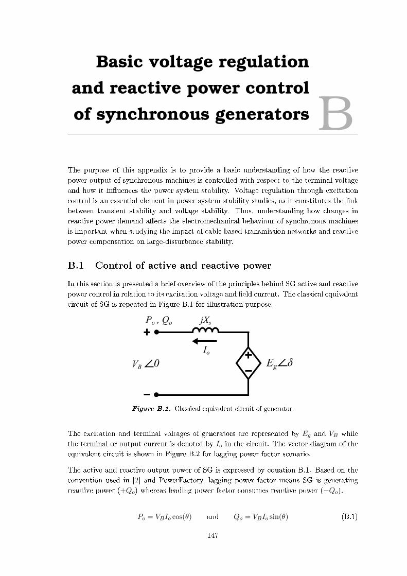
Basic voltage regulationand reactive power controlof synchronous generators B

The purpose of this appendix is to provide a basic understanding of how the reactive

power output of synchronous machines is controlled with respect to the terminal voltage

and how it inuences the power system stability. Voltage regulation through excitation

control is an essential element in power system stability studies, as it constitutes the link

between transient stability and voltage stability. Thus, understanding how changes in

reactive power demand aects the electromechanical behaviour of synchronous machines

is important when studying the impact of cable based transmission networks and reactive

power compensation on large-disturbance stability.

B.1 Control of active and reactive power

In this section is presented a brief overview of the principles behind SG active and reactive

power control in relation to its excitation voltage and eld current. The classical equivalent

circuit of SG is repeated in Figure B.1 for illustration purpose.

jXs

Eg δVB 0Io

Po , Qo

Figure B.1. Classical equivalent circuit of generator.

The excitation and terminal voltages of generators are represented by Eg and VB while

the terminal or output current is denoted by Io in the circuit. The vector diagram of the

equivalent circuit is shown in Figure B.2 for lagging power factor scenario.

The active and reactive output power of SG is expressed by equation B.1. Based on the

convention used in [2] and PowerFactory, lagging power factor means SG is generating

reactive power (+Qo) whereas leading power factor consumes reactive power (−Qo).

Po = VBIo cos(θ) and Qo = VBIo sin(θ) (B.1)

147

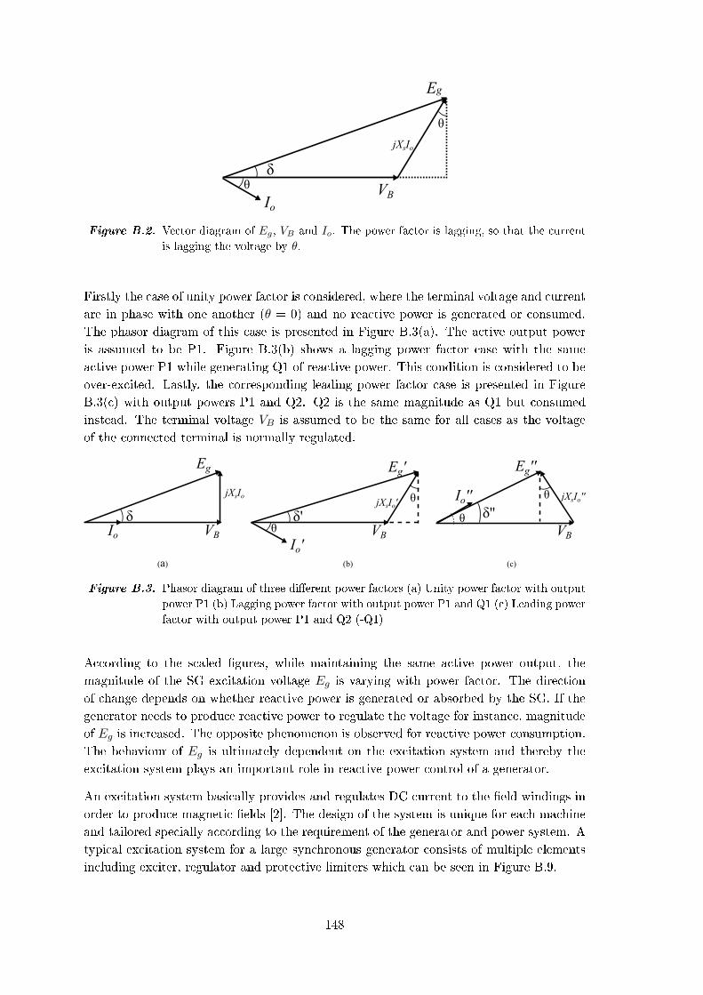
θ

θ

δ

Eg

VBIo

jXsIo

Figure B.2. Vector diagram of Eg, VB and Io. The power factor is lagging, so that the current

is lagging the voltage by θ.

Firstly the case of unity power factor is considered, where the terminal voltage and current

are in phase with one another (θ = 0) and no reactive power is generated or consumed.

The phasor diagram of this case is presented in Figure B.3(a). The active output power

is assumed to be P1. Figure B.3(b) shows a lagging power factor case with the same

active power P1 while generating Q1 of reactive power. This condition is considered to be

over-excited. Lastly, the corresponding leading power factor case is presented in Figure

B.3(c) with output powers P1 and Q2. Q2 is the same magnitude as Q1 but consumed

instead. The terminal voltage VB is assumed to be the same for all cases as the voltage

of the connected terminal is normally regulated.

δ

Eg

VBIo

jXsIo

(a)

δ'

Eg'

VB

jXsIo'

(b)

θ

Io'

δ''

Eg''

VB

jXsIo''

(c)

θ

Io''θ θ

Figure B.3. Phasor diagram of three dierent power factors (a) Unity power factor with output

power P1 (b) Lagging power factor with output power P1 and Q1 (c) Leading power

factor with output power P1 and Q2 (-Q1)

According to the scaled gures, while maintaining the same active power output, the

magnitude of the SG excitation voltage Eg is varying with power factor. The direction

of change depends on whether reactive power is generated or absorbed by the SG. If the

generator needs to produce reactive power to regulate the voltage for instance, magnitude

of Eg is increased. The opposite phenomenon is observed for reactive power consumption.

The behaviour of Eg is ultimately dependent on the excitation system and thereby the

excitation system plays an important role in reactive power control of a generator.

An excitation system basically provides and regulates DC current to the eld windings in

order to produce magnetic elds [2]. The design of the system is unique for each machine

and tailored specially according to the requirement of the generator and power system. A

typical excitation system for a large synchronous generator consists of multiple elements

including exciter, regulator and protective limiters which can be seen in Figure B.9.

148

The exciter is the element that is responsible for providing DC current to the eld windings

and thus controlling the excitation voltage. The relationship between eld current If and

excitation voltage Eg is shown in B.2, whereby magnetic saturation is neglected. M refers

to the mutual inductance between stator and rotor and ωs is synchronous speed. Both of

these are constant parameters and therefore constituting a linear form of relationship.

Eg,rms =ωsMIf√

2(B.2)

With equation B.2 being established, it is then possible to showcase the eects of power

control on eld current If . Figure B.4 shows the phasor diagram of two over-excited cases

with a constant lagging power factor. It can be seen that an increment in output power

is followed by increasing magnitude of Eg thereby If also rises proportionally.

δ

Eg

VB

jXsIo

θ

Io

θ

Io'

Eg'

jXsIo'

δ'

Figure B.4. Phasor diagram of constant power factor over-excitation cases. The power factor

is lagging, so that the current is lagging the voltage by θ. Dotted line refers to a

higher power operating state.

However for under-excited cases with a constant leading power factor the relationship

is not as straightforward. Referring to Figure B.5, starting from a low operating point,

increasing output magnitude would result in an initial decrease in Eg up to a minimum

point. Beyond this point the magnitude of Eg would begin to increase back again together

with the increment in output power. This explains the shape of the dotted red lines shown

in Figure B.6. This is only observed when the generator is operating under power factor

control.

As for voltage control operation where the active power is kept constant while reactive

power is varied accordingly, Eg and If tend to increase during over-excited conditions

within the operating limits and vice versa. The general behaviour of eld current If with

respect to power control of the generator can be summarized by the Io-If curves presented

in Figure B.6 [2]. Output current Io is analogous to output power magnitude assuming

constant terminal voltage VB.

149

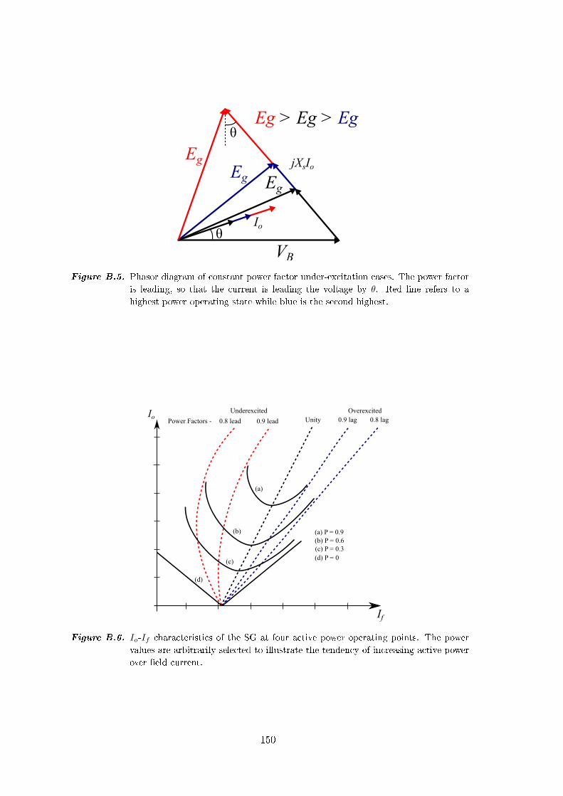
VB

θ Io

jXsIo

EgEg

Eg > Eg > Egθ

Eg

Figure B.5. Phasor diagram of constant power factor under-excitation cases. The power factor

is leading, so that the current is leading the voltage by θ. Red line refers to a

highest power operating state while blue is the second highest.

Io

If

0.8 lead 0.9 lead 0.9 lag 0.8 lagUnityPower Factors -

Underexcited Overexcited

(a)

(b)

(c)

(d)

(d) P = 0(c) P = 0.3(b) P = 0.6(a) P = 0.9

Figure B.6. Io-If characteristics of the SG at four active power operating points. The power

values are arbitrarily selected to illustrate the tendency of increasing active power

over eld current.

150

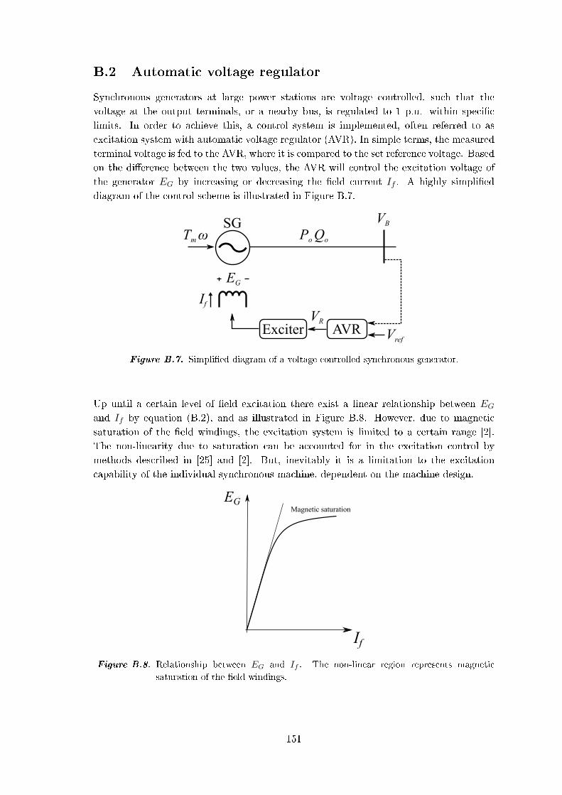
B.2 Automatic voltage regulator

Synchronous generators at large power stations are voltage controlled, such that the

voltage at the output terminals, or a nearby bus, is regulated to 1 p.u. within specic

limits. In order to achieve this, a control system is implemented, often referred to as

excitation system with automatic voltage regulator (AVR). In simple terms, the measured

terminal voltage is fed to the AVR, where it is compared to the set reference voltage. Based

on the dierence between the two values, the AVR will control the excitation voltage of

the generator EG by increasing or decreasing the eld current If . A highly simplied

diagram of the control scheme is illustrated in Figure B.7.

SGTm ω

AVR VrefExciter

EG

If

VR

Po Qo

VB

Figure B.7. Simplied diagram of a voltage controlled synchronous generator.

Up until a certain level of eld excitation there exist a linear relationship between EGand If by equation (B.2), and as illustrated in Figure B.8. However, due to magnetic

saturation of the eld windings, the excitation system is limited to a certain range [2].

The non-linearity due to saturation can be accounted for in the excitation control by

methods described in [25] and [2]. But, inevitably it is a limitation to the excitation

capability of the individual synchronous machine, dependent on the machine design.

EG

If

Magnetic saturation

Figure B.8. Relationship between EG and If . The non-linear region represents magnetic

saturation of the eld windings.

151

Figure B.9 show a more detailed, but yet simplied block diagram of a voltage regulated

excitation system. The elements of the block diagram are chosen based on the most

essential components described in [43]. Describing the system from the left to the right of

Figure B.9:

1. The control system receives the measured terminal voltage of the synchronous

generator as control signal. The signal is delayed by a rst order delay, which

represent any measurement time delay in the system.

2. A signal error is calculated by comparison with the reference voltage value (1 p.u.),

while accounting for possible input signals from over-excitation limiter (OEL) or

under-excitation limiter (UEL).

3. At the next summing junction, the signal is regulated by a stabilizing feedback Vfand a possible input from a power system stabilizer (PSS) if implemented. The

feedback is a rst-order lag controller, which stabilizes the AVR system by reducing

any steady state error in the signal.

4. Amplier: A rst-order forward regulator with gain KA and time constant TA. The

main function of this element is to amplify the control signal for the excitation

system to change the eld current If . The limits VR,MAX and VR,MIN incorporates

limitations to the amplier power supply or possible saturation [43].

5. The excitation system of the synchronous generator which can be designed in several

ways. Examples of both DC and AC excitation systems are given in [2] and [25].

However, the main purpose is to produce the DC eld current If in the eld windings

of the rotor to produce the excitation voltage EG. The excitation has gain KE and

time constant TE .

EG

If

VR

Field Armature

Synchronous generator Vref

∑

Vpss

Verr

VOEL VUEL

11+sT

VF

VB

TE∑

sKF

1+sTF

KA

1+sTA

VR,MIN

VR,MAX

VB

KE,

Figure B.9. AVR and excitation system with feedback control and amplier.

B.3 Excitation system inuence on power system stability

The speed and maximum level of the excitation system are of great importance for the

transient stability of the power system [25]. If the voltage VB at the terminals of the

synchronous generator drops due to a faulted condition, EG must be increased in order

to supply active and reactive power to maintain voltage at a reasonable level. When the

fault is removed by switching of a line, the thevenin equivalent impedance seen by the

generator changes, and the excitation system must react.

152

Thus, the described AVR and excitation system illustrated in Figure B.9 must be able

to respond as fast as possible with low time constants TA and TE . Standard values

for TA and TE in the IEEEX1 excitation system are 0.2 s and 0.5 s respectively, with a

measurement delay 1 ms. Besides speed, the maximum possible excitation level of EGis of great importance, also referred to as ceiling value. Imagining an excitation system

which reacts instantaneously, with a total time constant of 0 s, and with no limitation to

EG, then there would not exist a P, δ stability limit, and the terminal voltage VB would

be kept at 1 p.u. in any operating condition [25]. During electromechanical transients

following large disturbances, the synchronous generators experience P, δ-oscillations as it

is described in Section 1.3. If the excitation system is to slow, it will have a destabilizing

eect on the system, as the delayed control will interact with the system oscillations.

Thus, the delay of poorly designed excitation systems can in some cases result in worse

oscillations, than if the SG excitation was uncontrolled [25].

0 0.5 1 1.5 2 2.5 3 3.5 4 4.5

Time, t [s]

1

2

3

4

5

6

7

SG

exc

itatio

n vo

ltage

in p

.u. No AVR

IEEEX1DC2AAC2AST2A

0 0.5 1 1.5 2 2.5 3 3.5 4 4.5

Time, t [s]

0.2

0.3

0.4

0.5

0.6

0.7

0.8

0.9

1

1.1

SG

term

inal

vol

tage

in p

.u.

No AVRIEEEX1DC2AAC2AST2A

Figure B.10. Time response of EG and VB of SG2 following a three-phase fault on Line 4 in

the IEEE 9-bus system. The fault is kept for 60 ms, after which Line 4 is taken

out of service. Various cases of AVR systems are displayed according to [43].

IEEEX1: The 1979 IEEE type 1 (IEEEX1) excitation system model corresponds

to the 1981 IEEE type DC1 model. Field-controlled DC commutator exciters with

continuously acting voltage regulator. Few new synchronous machines are being

equipped with Type DC exciters, which have been superseded by AC and ST

systems. However many such systems are still in service [43].

DC2A: Field-controlled DC commutator exciters with continuously acting voltage

regulators. It diers from the Type DC1A model only in the voltage regulator output

limits, which are now proportional to terminal voltage.

AC2A: These excitation systems use an AC-alternator and either stationary or

rotating rectiers to produce the DC eld required [43].

ST2A: Static excitation system model utilizing both current and voltage sources

(generator terminal quantities) to control the excitation. In these excitation systems,

voltage and current is transformed to an appropriate level. Rectiers, either

controlled or non-controlled, provide the necessary direct current for the generator

eld. For many of the static systems, exciter ceiling voltage is very high. For such

systems, additional eld current limiter circuits may be used to protect the exciter

and the generator rotor [43].

153

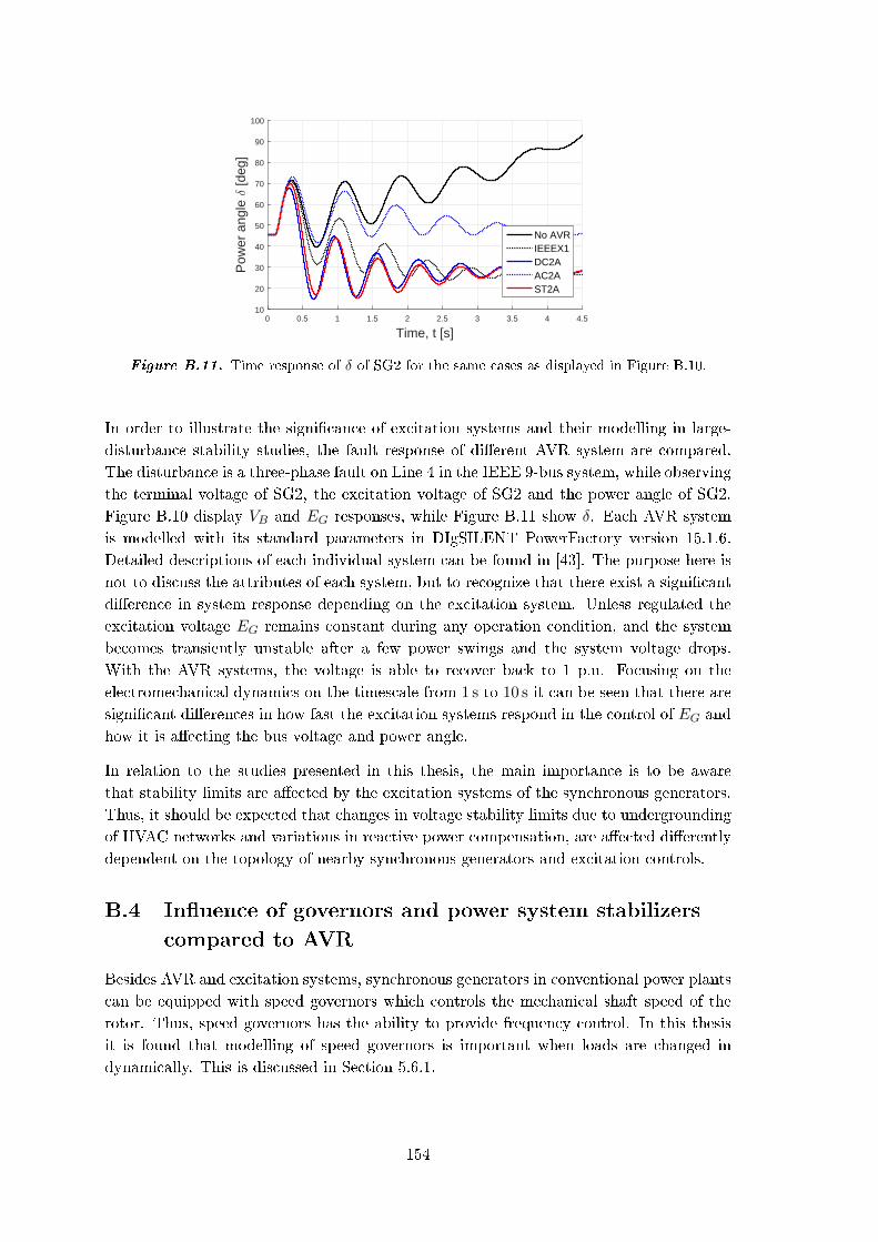
0 0.5 1 1.5 2 2.5 3 3.5 4 4.5

Time, t [s]

10

20

30

40

50

60

70

80

90

100

Pow

er a

ngle

δ [d

eg]

No AVRIEEEX1DC2AAC2AST2A

Figure B.11. Time response of δ of SG2 for the same cases as displayed in Figure B.10.

In order to illustrate the signicance of excitation systems and their modelling in large-

disturbance stability studies, the fault response of dierent AVR system are compared.

The disturbance is a three-phase fault on Line 4 in the IEEE 9-bus system, while observing

the terminal voltage of SG2, the excitation voltage of SG2 and the power angle of SG2.

Figure B.10 display VB and EG responses, while Figure B.11 show δ. Each AVR system

is modelled with its standard parameters in DIgSILENT PowerFactory version 15.1.6.

Detailed descriptions of each individual system can be found in [43]. The purpose here is

not to discuss the attributes of each system, but to recognize that there exist a signicant

dierence in system response depending on the excitation system. Unless regulated the

excitation voltage EG remains constant during any operation condition, and the system

becomes transiently unstable after a few power swings and the system voltage drops.

With the AVR systems, the voltage is able to recover back to 1 p.u. Focusing on the

electromechanical dynamics on the timescale from 1 s to 10 s it can be seen that there are

signicant dierences in how fast the excitation systems respond in the control of EG and

how it is aecting the bus voltage and power angle.

In relation to the studies presented in this thesis, the main importance is to be aware

that stability limits are aected by the excitation systems of the synchronous generators.

Thus, it should be expected that changes in voltage stability limits due to undergrounding

of HVAC networks and variations in reactive power compensation, are aected dierently

dependent on the topology of nearby synchronous generators and excitation controls.

B.4 Inuence of governors and power system stabilizers

compared to AVR

Besides AVR and excitation systems, synchronous generators in conventional power plants

can be equipped with speed governors which controls the mechanical shaft speed of the

rotor. Thus, speed governors has the ability to provide frequency control. In this thesis

it is found that modelling of speed governors is important when loads are changed in

dynamically. This is discussed in Section 5.6.1.

154

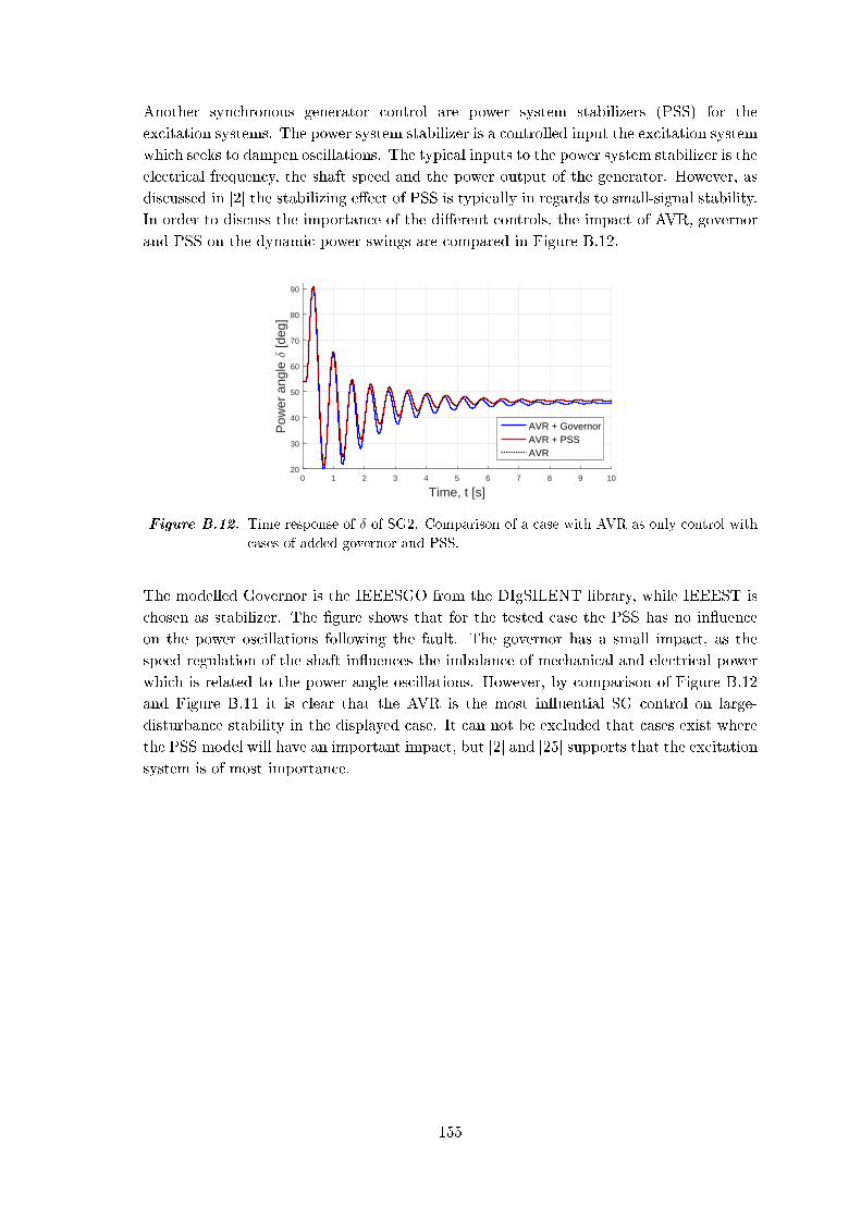
Another synchronous generator control are power system stabilizers (PSS) for the

excitation systems. The power system stabilizer is a controlled input the excitation system

which seeks to dampen oscillations. The typical inputs to the power system stabilizer is the

electrical frequency, the shaft speed and the power output of the generator. However, as

discussed in [2] the stabilizing eect of PSS is typically in regards to small-signal stability.

In order to discuss the importance of the dierent controls, the impact of AVR, governor

and PSS on the dynamic power swings are compared in Figure B.12.

0 1 2 3 4 5 6 7 8 9 10

Time, t [s]

20

30

40

50

60

70

80

90P

ower

ang

le δ

[deg

]

AVR + GovernorAVR + PSSAVR

Figure B.12. Time response of δ of SG2. Comparison of a case with AVR as only control with

cases of added governor and PSS.

The modelled Governor is the IEEESGO from the DIgSILENT library, while IEEEST is

chosen as stabilizer. The gure shows that for the tested case the PSS has no inuence

on the power oscillations following the fault. The governor has a small impact, as the

speed regulation of the shaft inuences the imbalance of mechanical and electrical power

which is related to the power angle oscillations. However, by comparison of Figure B.12

and Figure B.11 it is clear that the AVR is the most inuential SG control on large-

disturbance stability in the displayed case. It can not be excluded that cases exist where

the PSS model will have an important impact, but [2] and [25] supports that the excitation

system is of most importance.

155

Modelling parameters in9-bus and 39-bus systems C

This appendix is done for reference purpose of the test systems used in the thesis. Both

9-bus and 39-bus system models are obtained directly from PowerFactory with a certain

set of element parameters. Nonetheless the only elements included in this appendix are

line, synchronous generator (SG) and load.

For the line element, the parameters shown are as follow:

Terminal i and j: Terminals to which the line is connected

Length: Total length of the line

R: AC resistance at 20 per-km

L: Line inductance per-km

C : Line capacitance per-km

As for the SG element, the parameters shown are as follow:

Sn and Vn: Nominal power and voltage ratings

H : Inertia time constant of the machine

P : Active power dispatch

Vset: Voltage setpoint for voltage control mode

Finally, for the load element, the parameters shown are as follow:

P : Nominal active power

Q: Nominal reactive power

Power Factor: Nominal Power factor

C.1 9-bus system

With reference to Figure 4.1, the parameters of each line is shown in Table C.1.

Table C.2 presents the steady-state parameters and the inertia constant, H of the SGs in

the system. The dynamic modelling parameters of the generator models are not included

in the table. In PowerFactory version 15.2, there are two types of SG model available

in the RMS simulation tab: Classical and Detailed. Detailed model includes transient

and subtransient modelling (dq0) which is not included in classical model. Choosing

the classical mode yields coherent results as in [25] from which the IEEE 9-bus is rst

introduced with classical representation of SG for transient stability study. On the other

hand, the SG models used in the project are taken from version 15.1 which only includes

the detailed model. Therefore there exists a dierence between the results in this project

and in [25] even when subjected to the same disturbance.

157

One important dierence in the AVR design between the generators is that G1 and G3

have a very low gain KA as shown in Figure B.7 which renders the excitation system

insignicant during the transient period. It is fair to conclude that only G2 has an active

excitation system.

Lastly the load parameters are presented in Table C.3.

Table C.1. Line parameters of 9-bus model

Line Terminal i Terminal j Length [km] R [Ω/km] L [mH/km] C [µF/km]

Line 1 Bus 5 Bus 4 100 0.0529 1.431 0.01059

Line 2 Bus 7 Bus 5 100 0.1693 2.711 0.01841

Line 3 Bus 7 Bus 8 100 0.0449 1.212 0.00896

Line 4 Bus 8 Bus 9 100 0.0629 1.697 0.01257

Line 5 Bus 9 Bus 6 100 0.2063 2.862 0.02154

Line 6 Bus 6 Bus 4 100 0.0899 1.549 0.00951

Table C.2. Generator parameters of 9-bus model

Generator Sn [MVA] Vn [kV] H [s] P [MW] Vset in p.u.

G1 247.5 16.5 4.775 163 1.04

G2 192 18.0 1.77 163 1.025

G3 128 13.8 1.175 85 1.025

Table C.3. Load parameters of 9-bus model

Load P [MW] Q [Mvar] Power Factor

A 125 50 0.928 ind.

B 90 30 0.948 ind.

C 100 35 0.943 ind.

158

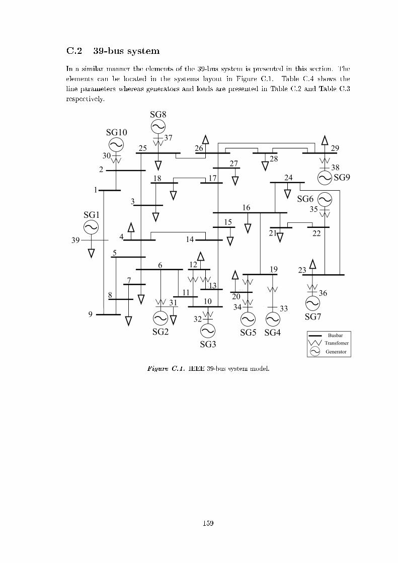
C.2 39-bus system

In a similar manner the elements of the 39-bus system is presented in this section. The

elements can be located in the systems layout in Figure C.1. Table C.4 shows the

line parameters whereas generators and loads are presented in Table C.2 and Table C.3

respectively.

3725

30

2

39

9

26

18

3

4

5

7

8

17

14

6

3111

10

32

12

13

15

16

2728

29

3824

35

21 22

23

36

33

19

20

Busbar

Transfomer

Generator

1

34

SG10

SG8

SG1

SG2SG3

SG5 SG4

SG7

SG9

SG6

Figure C.1. IEEE 39-bus system model.

159

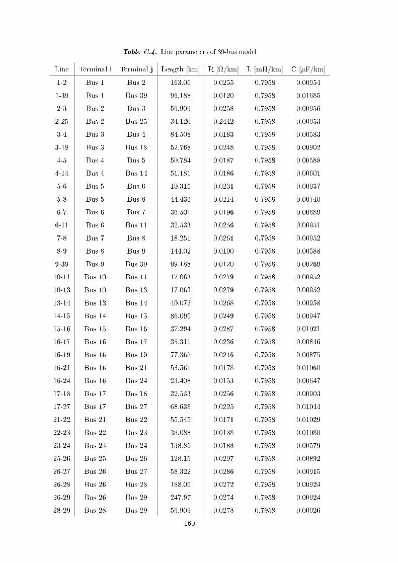
Table C.4. Line parameters of 39-bus model

Line Terminal i Terminal j Length [km] R [Ω/km] L [mH/km] C [µF/km]

1-2 Bus 1 Bus 2 163.06 0.0255 0.7958 0.00954

1-39 Bus 1 Bus 39 99.188 0.0120 0.7958 0.01685

2-3 Bus 2 Bus 3 59.909 0.0258 0.7958 0.00956

2-25 Bus 2 Bus 25 34.120 0.2442 0.7958 0.00953

3-4 Bus 3 Bus 4 84.508 0.0183 0.7958 0.00583

3-18 Bus 3 Bus 18 52.768 0.0248 0.7958 0.00902

4-5 Bus 4 Bus 5 50.784 0.0187 0.7958 0.00588

4-14 Bus 4 Bus 14 51.181 0.0186 0.7958 0.00601

5-6 Bus 5 Bus 6 10.316 0.0231 0.7958 0.00937

5-8 Bus 5 Bus 8 44.436 0.0214 0.7958 0.00740

6-7 Bus 6 Bus 7 36.501 0.0196 0.7958 0.00689

6-11 Bus 6 Bus 11 32.533 0.0256 0.7958 0.00951

7-8 Bus 7 Bus 8 18.251 0.0261 0.7958 0.00952

8-9 Bus 8 Bus 9 144.02 0.0190 0.7958 0.00588

9-39 Bus 9 Bus 39 99.188 0.0120 0.7958 0.00269

10-11 Bus 10 Bus 11 17.063 0.0279 0.7958 0.00952

10-13 Bus 10 Bus 13 17.063 0.0279 0.7958 0.00952

13-14 Bus 13 Bus 14 40.072 0.0268 0.7958 0.00958

14-15 Bus 14 Bus 15 86.095 0.0249 0.7958 0.00947

15-16 Bus 15 Bus 16 37.294 0.0287 0.7958 0.01021

16-17 Bus 16 Bus 17 35.311 0.0236 0.7958 0.00846

16-19 Bus 16 Bus 19 77.366 0.0246 0.7958 0.00875

16-21 Bus 16 Bus 21 53.561 0.0178 0.7958 0.01060

16-24 Bus 16 Bus 24 23.408 0.0153 0.7958 0.00647

17-18 Bus 17 Bus 18 32.533 0.0256 0.7958 0.00903

17-27 Bus 17 Bus 27 68.638 0.0225 0.7958 0.01044

21-22 Bus 21 Bus 22 55.545 0.0171 0.7958 0.01029

22-23 Bus 22 Bus 23 38.088 0.0188 0.7958 0.01080

23-24 Bus 23 Bus 24 138.86 0.0188 0.7958 0.00579

25-26 Bus 25 Bus 26 128.15 0.0297 0.7958 0.00892

26-27 Bus 26 Bus 27 58.322 0.0286 0.7958 0.00915

26-28 Bus 26 Bus 28 188.06 0.0272 0.7958 0.00924

26-29 Bus 26 Bus 29 247.97 0.0274 0.7958 0.00924

28-29 Bus 28 Bus 29 59.909 0.0278 0.7958 0.00926

160

Table C.5. Generator parameters of 39-bus model

Generator Sn [MVA] Vn [kV] H [s] P [MW] Vset in p.u.

SG1 10000 345 5 1000 1.03

SG2 700 16.5 4.329 520.8 0.982

SG3 800 16.5 4.475 650 0.9831

SG4 800 16.5 3.575 632 0.9972

SG5 300 16.5 4.333 254 1.0123

SG6 800 16.5 4.35 650 1.0493

SG7 700 16.5 3.771 560 1.0635

SG8 700 16.5 3.471 540 1.0278

SG9 1000 16.5 3.45 830 1.0265

SG10 1000 16.5 4.2 250 1.0475

Table C.6. Load parameters of 39-bus model

Load P [MW] Q [Mvar] Power Factor

3 322 2.4 0.99997 ind.

4 500 184 0.93847 ind.

7 233.8 84. 0.94110 ind.

8 522 176. 0.94758 ind.

12 7.5 88. 0.08491 ind.

15 320 153 0.90218 ind.

16 329 32.3 0.99521 ind.

18 158 30 0.98244 ind.

20 628 103 0.98681 ind.

21 274 115 0.92207 ind.

23 247.5 84.6 0.94624 ind.

24 308.6 -92.2 0.95815 cap.

25 224 47.2 0.97851 ind.

26 139 17 0.99260 ind.

27 281 75.5 0.96574 ind.

28 206 27.6 0.99114 ind.

29 283.5 26.9 0.99552 ind.

31 9.2 4.6 0.89442 ind.

39 1104 250 0.97530 ind.

161

DIgSILENT ProgrammingLanguage used in studies D

This appendix presents the DIgSILENT Programming Language (DPL) scripts that have

been used to obtain the critical clearing time in transient stability analysis of IEEE 9-bus

and 39-bus system. Three DPL scripts of coding that are used extensively throughout are

labelled as LineSweep, CCT and AngleLimit. LineSweep is the main script and CCT and

AngleLimit are sub-scripts that are automatically executed within the main script.

LineSweep: DPL script for sweeping across all the lines in the system

set S_gen , L , Events ; % Def ine s e t v a r i a b l e s

double i , Step ; % Def ine double v a r i a b l e s

i n t Step_2 , Step_3 , p ; % Def ine i n t e g e r v a r a i b l e s

ob j e c t I n i t i a l , RMS, o_gen ; % Def ine ob j e c t v a r i a b l e s

ob j e c t o_result , o_clear ;

ob j e c t A, o_fault , o_trip , pEvent , f au l t , f_c l ea r ;

s t r i n g Name, Pathway ; % Def ine ob j e c t v a r i a b l e s

ClearOutput ( ) ; % Clear output window

EchoOff ( ) ; % Turn o f f g r aph i c a l i n t e r f a c e − speed up s imu la t i on

I n i t i a l = GetCaseCommand( 'ComInc ' ) ; % Assign i n i t i a l c ond i t i on s

RMS = GetCaseCommand( 'ComSim ' ) ; % Assign RMS s imu la t i on command

! Se t t i ng the sw i t ch ing event for f a u l t

pEvent = I n i t i a l : p_event ; % Assign event o f i n i t i a l i z a t i o n

Events=pEvent . GetContents ( ) ; % Assign s e t o f events

f a u l t = Events . F i r s t F i l t ( ' Fault ' ) ; % Assign f a u l t event

f_c l ea r = Events . F i r s t F i l t ( ' Clear ' ) ; % Assign f a u l t c l e a r i n g event

Pathway = OHL_Result : f_name ; % Folder pathway f o r sav ing r e s u l t s

L=Lines . Get ( ) ; % Assign s e t o f l i n e s

% Loop to change l o c a t i o n o f the f a u l t on the l i n e s (1% and 99%)

for (p=99; p<100; p=p+98)

% Reset t ing dp l l o f a l l l i n e s − d e s c r i p t i o n parameter o f the l i n e s

A=L . F i r s t ( ) ; % Assign A the f i r s t l i n e in l i n e s s e t

while (A)

A: dpl1=0; % Reset dp l l to 0

163

A: f s h c l o c = p ; % Set f a u l t l o c a t i o n

A=L . Next ( ) ; % Proceed with next l i n e in L s e t

% Se t t i ng up the s imu la t ing events f o r f i nd i n g CCT

A=L . F i r s t ( ) ; % F i r s t l i n e

while (A) % Loop over a l l l i n e s

f a u l t : p_target=A; % Assign f au l t e d l i n e

f_c l ea r : p_target=A; % Assign l i n e to be c l e a r ed

CCT. Execute ( ) ; % Execute CCT s c r i p t

A: dpl1=CCT: t_cr i t ; % Assign CCT to each l i n e

A: dpl1=A: dpl1 −0.1 ; % Minus durat ion be f o r e f a u l t

% Assign name f o r each r e s u l t f i l e

Name = sprintf ( '%s_%i_%s_%f_%i%s ' ,Pathway ,A: f s h c l o c ,A: loc_name ,

A: dpl1 ,CCT: Step , ' . csv ' ) ;

OHL_Result : f_name = Name ; % Assign r e s u l t export f i l e name

OHL_Result . Execute ( ) ; % Export as CSV f i l e

A=L . Next ( ) ; % Proceed with next l i n e

% Print the CCTs o f each l i n e at d i f f e r e n t l o c a t i o n s

A=L . F i r s t ( ) ;

while (A)

p r i n t f ( 'CCT o f %s with f a u l t at %i percent i s %5.3 f seconds ' ,

A: loc_name , A: f s h c l o c , A: dpl1 ) ;

A=L . Next ( ) ;

p r i n t f ( ' ' ) ;

p r i n t f ( '−−−−−−−−−−−−−−−−−−−−−−−−−−−−−−−−−−−−−−−−−−−−−−−−− ' ) ;

OHL_Result : f_name = Pathway ; % Reset path f o r r e s u l t command

CCT: DPL script for increasing fault time to obtain CCT

set Events ; % Def ine s e t v a r i a b l e s

double i ; % Def ine double v a r i a b l e s

ob j e c t I n i t i a l , RMS, Resu l t s ; % Def ine ob j e c t v a r i a b l e s

ob j e c t pEvent , f au l t , f_c l ea r ;

s t r i n g Name ; % Def ine s t r i n g v a r i a b l e s

EchoOff ( ) ; % Turn o f f user i n t e r f a c e to speed up proce s s

I n i t i a l = GetCaseCommand( 'ComInc ' ) ; % Assign i n i t i a l c ond i t i on

RMS = GetCaseCommand( 'ComSim ' ) ; % Assign RMS s imu la t i on

Resu l t s = I n i t i a l : p_resvar ; % Assign s imu la t i on r e s u l t f i l e

% Se t t i ng the swi t ch ing events f o r f a u l t

164

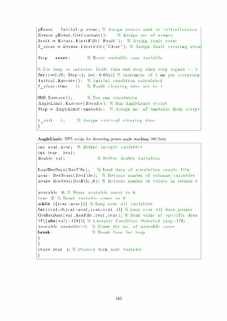
pEvent = I n i t i a l : p_event ; % Assign events used in i n i t i a l i z a t i o n

Events=pEvent . GetContents ( ) ; % Assign s e t o f events

f a u l t = Events . F i r s t F i l t ( ' Fault ' ) ; % Assign f a u l t event

f_c l ea r = Events . F i r s t F i l t ( ' Clear ' ) ; % Assign f a u l t c l e a r i n g event

Step = reset ; % Reset unstab l e case va r i ab l e

% For loop to i n c r e a s e f a u l t time and stop when step s i g n a l >= 1

for ( i =0.25; Step <1; i=i +0.001) % Increment o f 1 ms per i t e r a t i o n

I n i t i a l . Execute ( ) ; % I n i t i a l cond i t i on c a l c u l a t ed

f_c l ea r : time = i ; % Fault c l e a r i n g time s e t to i

RMS. Execute ( ) ; % Run rms s imu la t i on

AngleLimit . Execute ( Resu l t s ) ; % Run AngleLimit s c r i p t

Step = AngleLimit : unstab le ; % Assign no . o f unstab l e from s c r i p t

t_cr i t = i ; % Assign c r i t i c a l c l e a r i n g time

AngleLimit: DPL script for detecting power angle reaching 180 limit

i n t nval , nvar ; % Def ine i n t e g e r v a r i a b l e s

i n t ivar , i v a l ;

double va l ; % Def ine double v a r i a b l e s

LoadResData ( ResFi l e ) ; % Load data o f s imu la t i on r e s u l t f i l e

nvar= ResNvars ( ResFi l e ) ; % Returns number o f columns/ v a r i a b l e s

nval= ResNval ( ResFi le , 0 ) ; % Returns number o f va lue s in column 0

unstab le =0; % Reset unstab le count to 0

i va r =0; % Reset v a r i a b l e count to 0

while ( ivar<nvar ) % Loop over a l l v a r i a b l e s

for ( i v a l =0; i va l <nval ; i v a l=i v a l +1) % Loop over a l l data po in t s

GetResData ( val , ResFi le , i va l , i v a r ) ; % Read value at s p e c i f i c data

i f (abs ( va l )>179) % Unstable Condit ion Detected ( ang>179)

unstab le=unstab le +1; % Count the no . o f unstab le ca s e s

break ; % Break from f o r loop

i va r= iva r +1; % Proceed with next va r i ab l e

165

Pole-slip function inPowerFactory E

DIgSILENT PowerFactory has a built-in function for detection of pole-slip for transient

stability analysis. However, in the work presented in this thesis it was found that this tool

should be used with caution.

Prior to changing the CCT procedure in this thesis, the pole-slip function was utilized

in a DPL script to calculate CCT values. The script uses a function in the synchronous

machine, which changes a binary value from 0 to 1, if the machine loses synchronism.

This function is recognized as "out of step detection" or "pole-slip", and is dened in the

DIgSILENT documentation [36]. The DPL script runs a for-loop, which performs RMS

simulations while increasing the clearing time tc, and thus the fault duration tf . This

procedure is iterated until the pole-slip is detected, and the fault duration tf reached in

that iteration is the CCT.

An important note is that the pole-slip function is dened dierently depending on the

version of DIgSILENT PowerFactory. By correspondence with Stefan Weigel from the

DIgSILENT support on the 5th of April 2016, the following denition for pole-slip in

PowerFactory for all versions prior to 2016 was given:

"Till version 2016 the outofstep signal was calculated in a very simple, but not consistent

way: If the machine angle (rel) has two zero crossings in the same direction, then the

outofstep ag is set. This can mean that the outofstep ag is set in a range between 360

and 719 angle change. Dependent on the starting position of the machine angle (positive

or negative). This behavior was changed with version 2016 to a more consistent way".

In the 2016 version of the software, the out of step detection (pole-slip) is detected when

the rotor angle of the machine is changed 360 from its original operating point, with

reference to the local reference machine (in this case the innite bus).

Figure E.1 illustrates the dierence between the 2016 version of PowerFactory and older

versions. The consequence of the dierence is that CCT values calculated by the pole-

slip denition is dependent on the version of the software used. In the older versions

of PowerFactory the initial value of δ inuences the CCT directly, whereas the pole-slip

detection is independent of the initial value in version 2016. In any case the CCT will

always be inuenced by the initial power angle δ of the generator. The reason is that the

initial conditions inuence the P, δ characteristics and the change of states, illustrated in

Figure 1.9 in Section 1.3.1. In other words, the initial conditions should determine the

CCT together with the characteristics of the disturbance. However, the purpose of the

pole-slip function is to indicate when the machine is considered unstable beyond recovery.

167

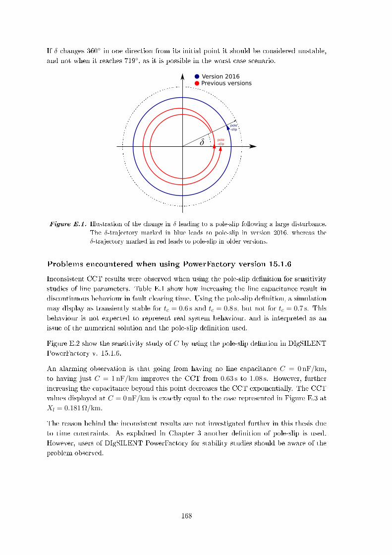
If δ changes 360 in one direction from its initial point it should be considered unstable,

and not when it reaches 719, as it is possible in the worst case scenario.

δ

pole-slip

pole-slip

Version 2016Previous versions

Figure E.1. Illustration of the change in δ leading to a pole-slip following a large disturbance.

The δ-trajectory marked in blue leads to pole-slip in version 2016, whereas the

δ-trajectory marked in red leads to pole-slip in older versions.

Problems encountered when using PowerFactory version 15.1.6

Inconsistent CCT results were observed when using the pole-slip denition for sensitivity

studies of line parameters. Table E.1 show how increasing the line capacitance result in

discontinuous behaviour in fault clearing time. Using the pole-slip denition, a simulation

may display as transiently stable for tc = 0.6 s and tc = 0.8 s, but not for tc = 0.7 s. This

behaviour is not expected to represent real system behaviour, and is interpreted as an

issue of the numerical solution and the pole-slip denition used.

Figure E.2 show the sensitivity study of C by using the pole-slip dention in DIgSILENT

PowerFactory v. 15.1.6.

An alarming observation is that going from having no line capacitance C = 0 nF/km,

to having just C = 1 nF/km improves the CCT from 0.63 s to 1.08 s. However, further

increasing the capacitance beyond this point decreases the CCT exponentially. The CCT

values displayed at C = 0 nF/km is exactly equal to the case represented in Figure E.3 at

Xl = 0.181 Ω/km.

The reason behind the inconsistent results are not investigated further in this thesis due

to time constraints. As explained in Chapter 3 another denition of pole-slip is used.

However, users of DIgSILENT PowerFactory for stability studies should be aware of the

problem observed.

168

Table E.1. Discontinuous behaviour of pole-slip detection

Clearing time, tc

0.5 s 0.6 s 0.7 s 0.8 s 0.9 s 1.0 s 1.1 s

Version 15.1.6

C = 0 nF X X 5 X X X 5

C = 1 nF X X 5 X X X 5

C = 100 nF X X X X 5 5 5

C = 200 nF X X 5 5 5 5 5

Version 2016

C = 0 nF X 5 5 5 5 5 5

C = 1 nF X 5 5 5 5 5 5

C = 100 nF 5 5 5 5 5 5 5

C = 200 nF X X 5 5 5 5 5

0 50 100 150 200 250 300 350 400

Transmission line capacitance, C [nF/km]

0.6

0.7

0.8

0.9

1

1.1

Critica

l cle

arin

g t

ime

, C

CT

[s]

df= 1 km

df= 99 km

0 nF/km

1 nF/km

Figure E.2. CCT sensitivity of line capacitance C in the SMIB system. The line is lossless, with

Xl = 0.181 Ω/km. Total length of the line, l = 100 km.

169

0.1 0.2 0.3 0.4 0.5 0.6 0.7 0.8 0.9 1

Line reactance, Xl [Ω/km]

0.45

0.5

0.55

0.6

0.65

0.7

Crit

ical

cle

arin

g tim

e, C

CT

[s]

df = 1 km

df = 99 km

Figure E.3. CCT sensitivity of line reactance Xl in the SMIB system. The line is purely

inductive, so that R = C = G = 0. Total length of the line, l = 100 km.

170

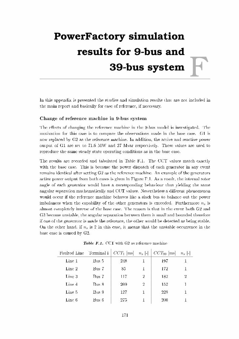
PowerFactory simulationresults for 9-bus and

39-bus system FIn this appendix is presented the studies and simulation results that are not included in

the main report and basically for ease of reference, if necessary.

Change of reference machine in 9-bus system

The eects of changing the reference machine in the 9-bus model is investigated. The

motivation for this case is to compare the observations made in the base case. G1 is

now replaced by G2 as the reference machine. In addition, the active and reactive power

output of G1 are set to 71.6 MW and 27 Mvar respectively. These values are used to

reproduce the same steady state operating conditions as in the base case.

The results are recorded and tabulated in Table F.1. The CCT values match exactly

with the base case. This is because the power dispatch of each generator in any event

remains identical after setting G2 as the reference machine. An example of the generators

active power output from both cases is given in Figure F.1. As a result, the internal rotor

angle of each generator would have a corresponding behaviour thus yielding the same

angular separation mathematically and CCT values. Nevertheless a dierent phenomenon

would occur if the reference machine behaves like a slack bus to balance out the power

imbalances when the capability of the other generators is exceeded. Furthermore ns is

almost completely inverse of the base case. The reason is that in the event both G2 and

G3 become unstable, the angular separation between them is small and bounded therefore

if one of the generator is made the reference, the other would be detected as being stable.

On the other hand, if ns is 2 in this case, it means that the unstable occurrence in the

base case is caused by G2.

Table F.1. CCT with G2 as reference machine

Faulted Line Terminal i CCT1 [ms] ns [-] CCT99 [ms] ns [-]

Line 1 Bus 5 248 1 197 1

Line 2 Bus 7 85 1 172 1

Line 3 Bus 7 117 2 182 2

Line 4 Bus 8 200 2 152 1

Line 5 Bus 9 127 1 228 1

Line 6 Bus 6 275 1 200 1

171

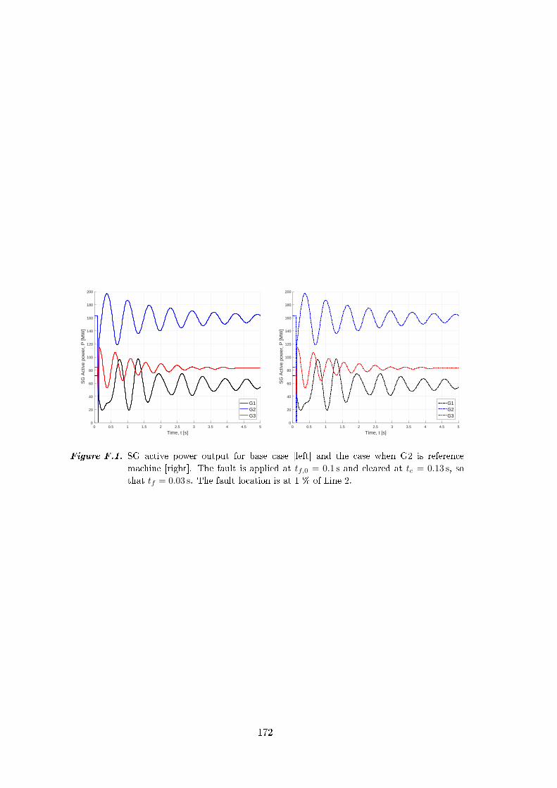
0 0.5 1 1.5 2 2.5 3 3.5 4 4.5 5

Time, t [s]

0

20

40

60

80

100

120

140

160

180

200

SG

Act

ive

pow

er, P

[MW

]

G1G2G3

0 0.5 1 1.5 2 2.5 3 3.5 4 4.5 5

Time, t [s]

0

20

40

60

80

100

120

140

160

180

200

SG

Act

ive

pow

er, P

[MW

]

G1G2G3

Figure F.1. SG active power output for base case [left] and the case when G2 is reference

machine [right]. The fault is applied at tf,0 = 0.1 s and cleared at tc = 0.13 s, so

that tf = 0.03 s. The fault location is at 1 % of Line 2.

172

Table F.2. CCT values of the base model in DIgSILENT PowerFactory.

Faulted Line Terminal i CCT1 [ms] ns [-] CCT99 [ms] ns [-]

1-2 Bus 1 639 1 197 1

1-39 Bus 1 630 1 851 1

2-3 Bus 2 264 1 317 2

2-25 Bus 2 158 1 115 2

3-4 Bus 3 315 2 263 1

3-18 Bus 3 315 1 307 1

4-5 Bus 4 279 2 239 2

4-14 Bus 4 287 1 284 1

5-6 Bus 5 239 2 227 2

5-8 Bus 5 253 2 300 2

6-7 Bus 6 238 2 301 2

6-11 Bus 6 236 1 234 1

7-8 Bus 7 304 1 300 2

8-9 Bus 8 298 1 848 1

9-39 Bus 9 863 1 960 1

10-11 Bus 10 217 1 238 1

10-13 Bus 10 209 1 233 1

13-14 Bus 13 224 1 254 1

14-15 Bus 14 266 1 285 2

15-16 Bus 15 272 1 173 4

16-17 Bus 16 136 2 197 1

16-19 Bus 16 191 1 358 1

16-21 Bus 16 144 1 172 2

16-24 Bus 16 183 1 224 1

17-18 Bus 17 227 1 295 1

17-27 Bus 17 241 1 201 1

21-22 Bus 21 108 2 92 2

22-23 Bus 22 202 1 188 1

23-24 Bus 23 170 2 198 1

25-26 Bus 25 206 1 125 1

26-27 Bus 26 139 1 211 1

26-28 Bus 26 110 1 102 1

26-29 Bus 26 96 1 71 1

28-29 Bus 28 68 1 53 1

173

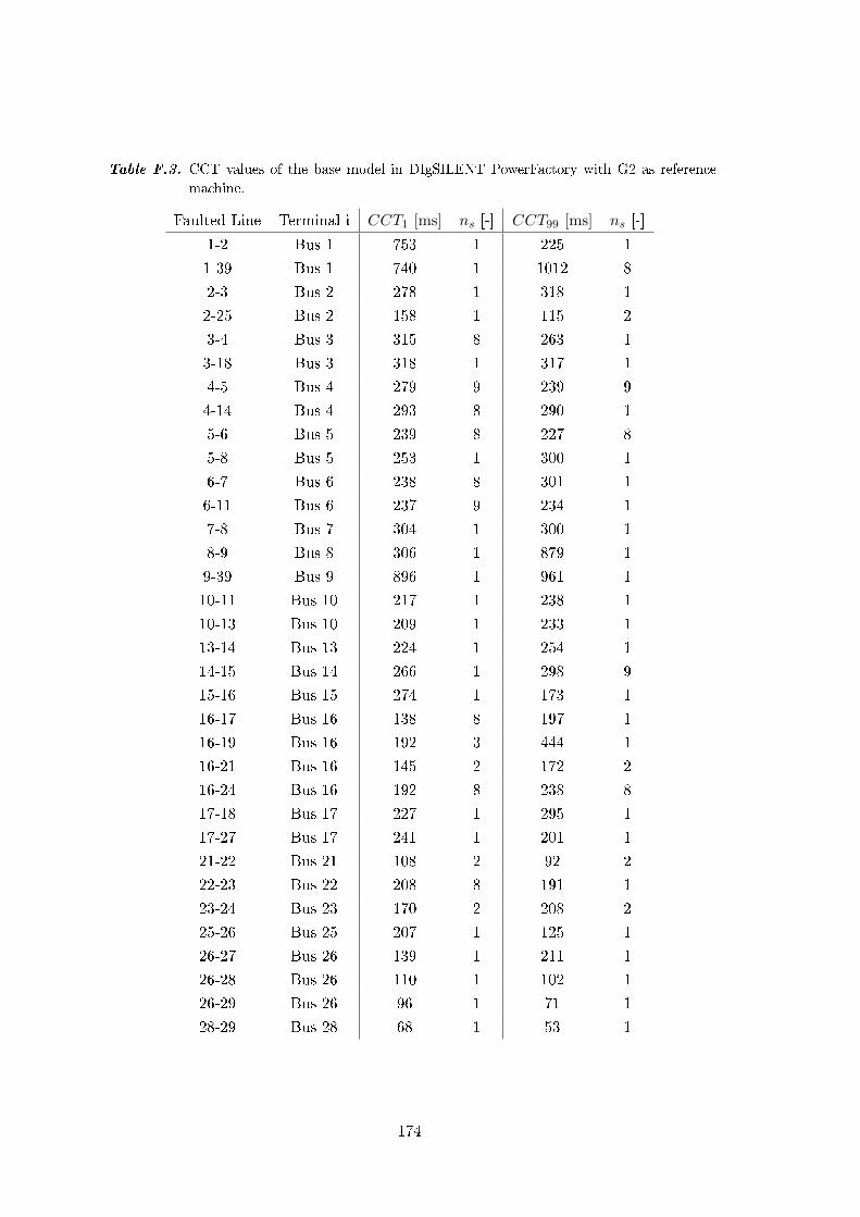
Table F.3. CCT values of the base model in DIgSILENT PowerFactory with G2 as reference

machine.

Faulted Line Terminal i CCT1 [ms] ns [-] CCT99 [ms] ns [-]

1-2 Bus 1 753 1 225 1

1-39 Bus 1 740 1 1012 8

2-3 Bus 2 278 1 318 1

2-25 Bus 2 158 1 115 2

3-4 Bus 3 315 8 263 1

3-18 Bus 3 318 1 317 1

4-5 Bus 4 279 9 239 9

4-14 Bus 4 293 8 290 1

5-6 Bus 5 239 8 227 8

5-8 Bus 5 253 1 300 1

6-7 Bus 6 238 8 301 1

6-11 Bus 6 237 9 234 1

7-8 Bus 7 304 1 300 1

8-9 Bus 8 306 1 879 1

9-39 Bus 9 896 1 961 1

10-11 Bus 10 217 1 238 1

10-13 Bus 10 209 1 233 1

13-14 Bus 13 224 1 254 1

14-15 Bus 14 266 1 298 9

15-16 Bus 15 274 1 173 1

16-17 Bus 16 138 8 197 1

16-19 Bus 16 192 3 444 1

16-21 Bus 16 145 2 172 2

16-24 Bus 16 192 8 238 8

17-18 Bus 17 227 1 295 1

17-27 Bus 17 241 1 201 1

21-22 Bus 21 108 2 92 2

22-23 Bus 22 208 8 191 1

23-24 Bus 23 170 2 208 2

25-26 Bus 25 207 1 125 1

26-27 Bus 26 139 1 211 1

26-28 Bus 26 110 1 102 1

26-29 Bus 26 96 1 71 1

28-29 Bus 28 68 1 53 1

174

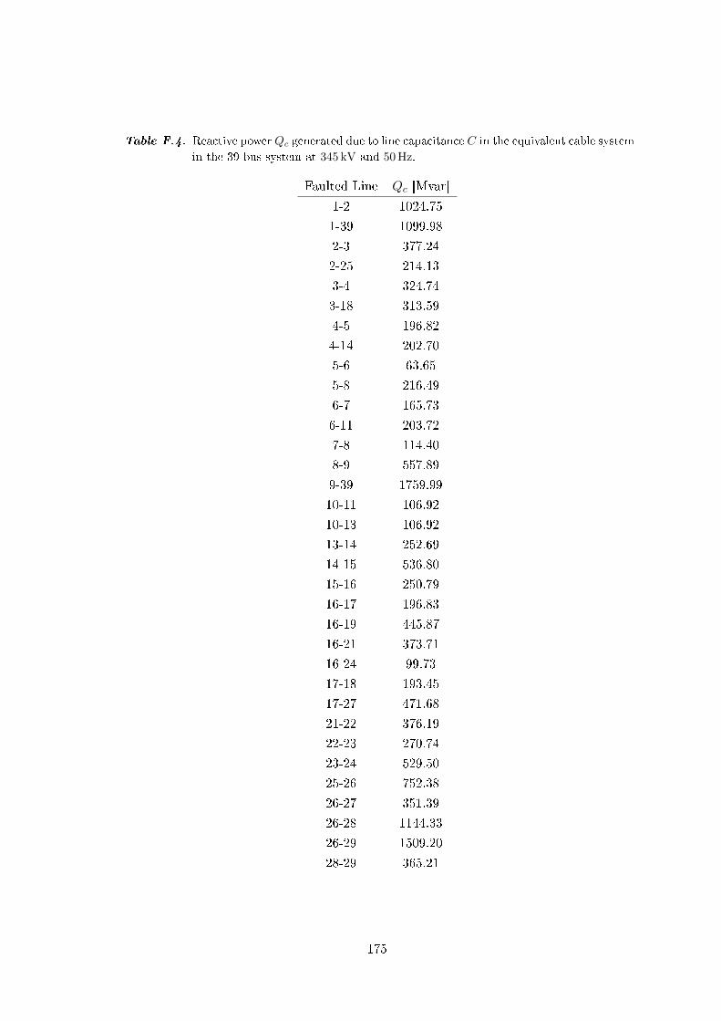
Table F.4. Reactive power Qc generated due to line capacitance C in the equivalent cable system

in the 39-bus system at 345 kV and 50 Hz.

Faulted Line Qc [Mvar]

1-2 1024.75

1-39 1099.98

2-3 377.24

2-25 214.13

3-4 324.74

3-18 313.59

4-5 196.82

4-14 202.70

5-6 63.65

5-8 216.49

6-7 165.73

6-11 203.72

7-8 114.40

8-9 557.89

9-39 1759.99

10-11 106.92

10-13 106.92

13-14 252.69

14-15 536.80

15-16 250.79

16-17 196.83

16-19 445.87

16-21 373.71

16-24 99.73

17-18 193.45

17-27 471.68

21-22 376.19

22-23 270.74

23-24 529.50

25-26 752.38

26-27 351.39

26-28 1144.33

26-29 1509.20

28-29 365.21

175

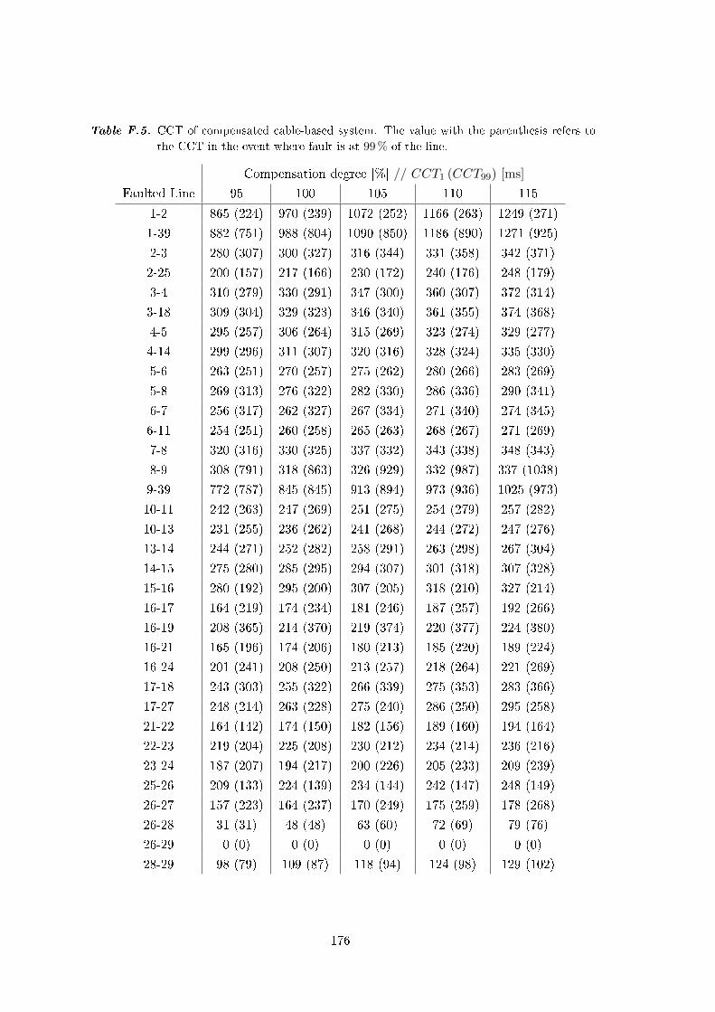
Table F.5. CCT of compensated cable-based system. The value with the parenthesis refers to

the CCT in the event where fault is at 99 % of the line.

Compensation degree [%] // CCT1 (CCT99) [ms]

Faulted Line 95 100 105 110 115

1-2 865 (224) 970 (239) 1072 (252) 1166 (263) 1249 (271)

1-39 882 (751) 988 (804) 1090 (850) 1186 (890) 1271 (925)

2-3 280 (307) 300 (327) 316 (344) 331 (358) 342 (371)

2-25 200 (157) 217 (166) 230 (172) 240 (176) 248 (179)

3-4 310 (279) 330 (291) 347 (300) 360 (307) 372 (314)

3-18 309 (304) 329 (323) 346 (340) 361 (355) 374 (368)

4-5 295 (257) 306 (264) 315 (269) 323 (274) 329 (277)

4-14 299 (296) 311 (307) 320 (316) 328 (324) 335 (330)

5-6 263 (251) 270 (257) 275 (262) 280 (266) 283 (269)

5-8 269 (313) 276 (322) 282 (330) 286 (336) 290 (341)

6-7 256 (317) 262 (327) 267 (334) 271 (340) 274 (345)

6-11 254 (251) 260 (258) 265 (263) 268 (267) 271 (269)

7-8 320 (316) 330 (325) 337 (332) 343 (338) 348 (343)

8-9 308 (791) 318 (863) 326 (929) 332 (987) 337 (1038)

9-39 772 (787) 845 (845) 913 (894) 973 (936) 1025 (973)

10-11 242 (263) 247 (269) 251 (275) 254 (279) 257 (282)

10-13 231 (255) 236 (262) 241 (268) 244 (272) 247 (276)

13-14 244 (271) 252 (282) 258 (291) 263 (298) 267 (304)

14-15 275 (280) 285 (295) 294 (307) 301 (318) 307 (328)

15-16 280 (192) 295 (200) 307 (205) 318 (210) 327 (214)

16-17 164 (219) 174 (234) 181 (246) 187 (257) 192 (266)

16-19 208 (365) 214 (370) 219 (374) 220 (377) 224 (380)

16-21 165 (196) 174 (206) 180 (213) 185 (220) 189 (224)

16-24 201 (241) 208 (250) 213 (257) 218 (264) 221 (269)

17-18 243 (303) 255 (322) 266 (339) 275 (353) 283 (366)

17-27 248 (214) 263 (228) 275 (240) 286 (250) 295 (258)

21-22 164 (142) 174 (150) 182 (156) 189 (160) 194 (164)

22-23 219 (204) 225 (208) 230 (212) 234 (214) 236 (216)

23-24 187 (207) 194 (217) 200 (226) 205 (233) 209 (239)

25-26 209 (133) 224 (139) 234 (144) 242 (147) 248 (149)

26-27 157 (223) 164 (237) 170 (249) 175 (259) 178 (268)

26-28 31 (31) 48 (48) 63 (60) 72 (69) 79 (76)

26-29 0 (0) 0 (0) 0 (0) 0 (0) 0 (0)

28-29 98 (79) 109 (87) 118 (94) 124 (98) 129 (102)

176

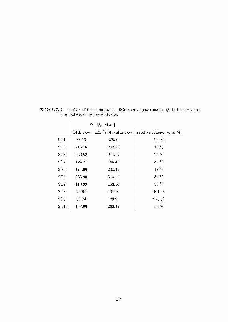
Table F.6. Comparison of the 39-bus system SGs reactive power output Qo in the OHL base

case and the equivalent cable case.

SG Qo [Mvar]

OHL case 100 % SR cable case relative dierence, dr %

SG1 88.15 325.6 269 %

SG2 213.16 242.85 14 %

SG3 222.52 271.19 22 %

SG4 124.27 186.42 50 %

SG5 171.86 200.35 17 %

SG6 233.96 313.79 34 %

SG7 113.99 153.50 35 %

SG8 21.68 108.70 401 %

SG9 57.74 189.91 229 %

SG10 168.06 262.43 56 %

177

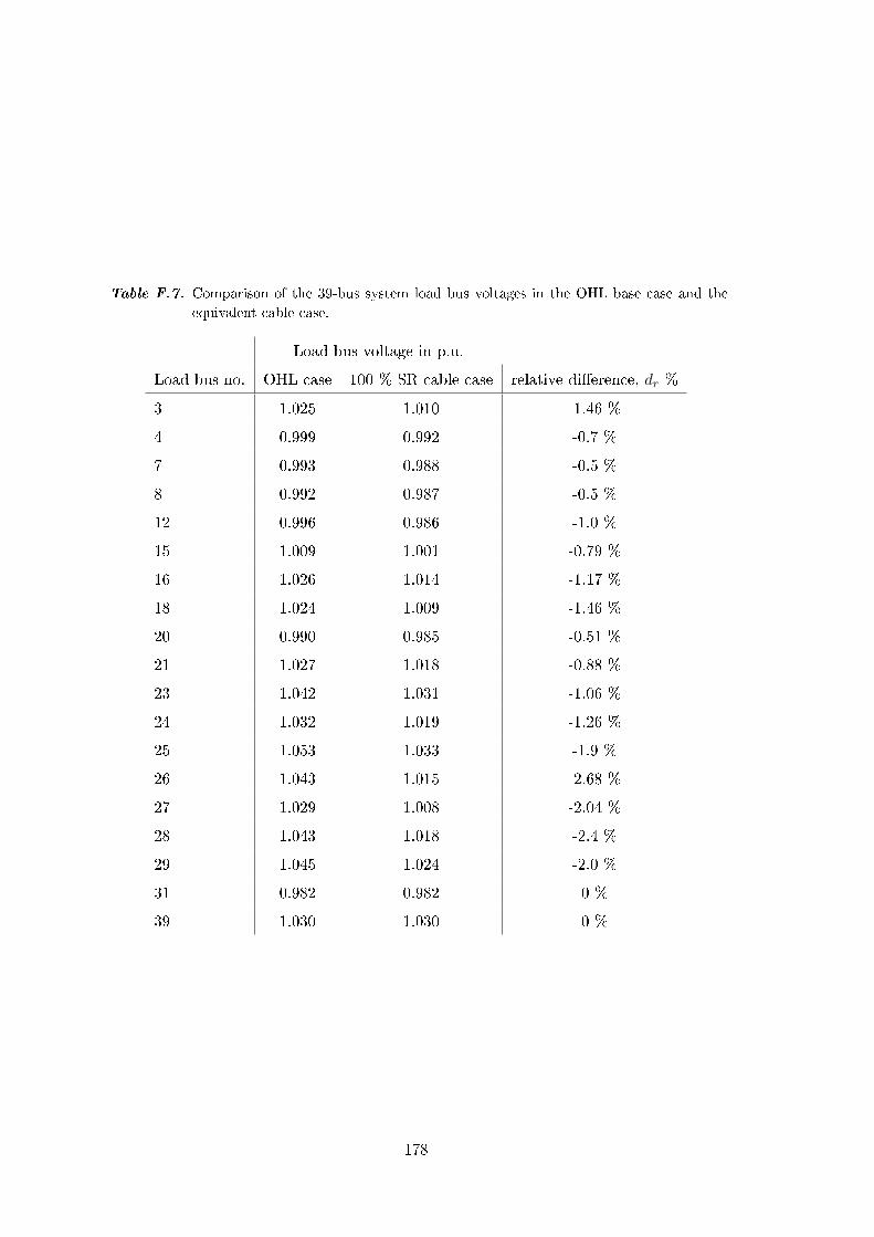
Table F.7. Comparison of the 39-bus system load bus voltages in the OHL base case and the

equivalent cable case.

Load bus voltage in p.u.

Load bus no. OHL case 100 % SR cable case relative dierence, dr %

3 1.025 1.010 -1.46 %

4 0.999 0.992 -0.7 %

7 0.993 0.988 -0.5 %

8 0.992 0.987 -0.5 %

12 0.996 0.986 -1.0 %

15 1.009 1.001 -0.79 %

16 1.026 1.014 -1.17 %

18 1.024 1.009 -1.46 %

20 0.990 0.985 -0.51 %

21 1.027 1.018 -0.88 %

23 1.042 1.031 -1.06 %

24 1.032 1.019 -1.26 %

25 1.053 1.033 -1.9 %

26 1.043 1.015 -2.68 %

27 1.029 1.008 -2.04 %

28 1.043 1.018 -2.4 %

29 1.045 1.024 -2.0 %

31 0.982 0.982 0 %

39 1.030 1.030 0 %

178

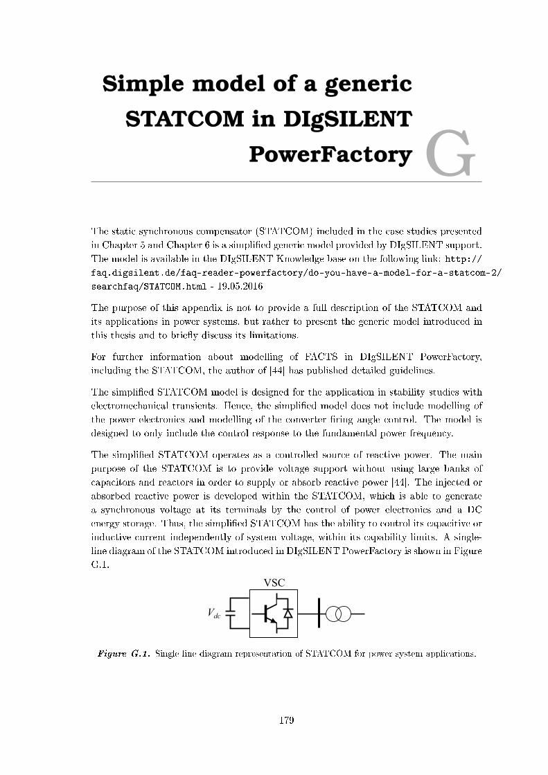
Simple model of a genericSTATCOM in DIgSILENT

PowerFactory GThe static synchronous compensator (STATCOM) included in the case studies presented

in Chapter 5 and Chapter 6 is a simplied generic model provided by DIgSILENT support.

The model is available in the DIgSILENT Knowledge base on the following link: http://

faq.digsilent.de/faq-reader-powerfactory/do-you-have-a-model-for-a-statcom-2/

searchfaq/STATCOM.html - 19.05.2016

The purpose of this appendix is not to provide a full description of the STATCOM and

its applications in power systems, but rather to present the generic model introduced in

this thesis and to briey discuss its limitations.

For further information about modelling of FACTS in DIgSILENT PowerFactory,

including the STATCOM, the author of [44] has published detailed guidelines.

The simplied STATCOM model is designed for the application in stability studies with

electromechanical transients. Hence, the simplied model does not include modelling of

the power electronics and modelling of the converter ring angle control. The model is

designed to only include the control response to the fundamental power frequency.

The simplied STATCOM operates as a controlled source of reactive power. The main

purpose of the STATCOM is to provide voltage support without using large banks of

capacitors and reactors in order to supply or absorb reactive power [44]. The injected or

absorbed reactive power is developed within the STATCOM, which is able to generate

a synchronous voltage at its terminals by the control of power electronics and a DC

energy storage. Thus, the simplied STATCOM has the ability to control its capacitive or

inductive current independently of system voltage, within its capability limits. A single-

line diagram of the STATCOM introduced in DIgSILENT PowerFactory is shown in Figure

G.1.

VSC

Vdc

Figure G.1. Single-line diagram representation of STATCOM for power system applications.

179

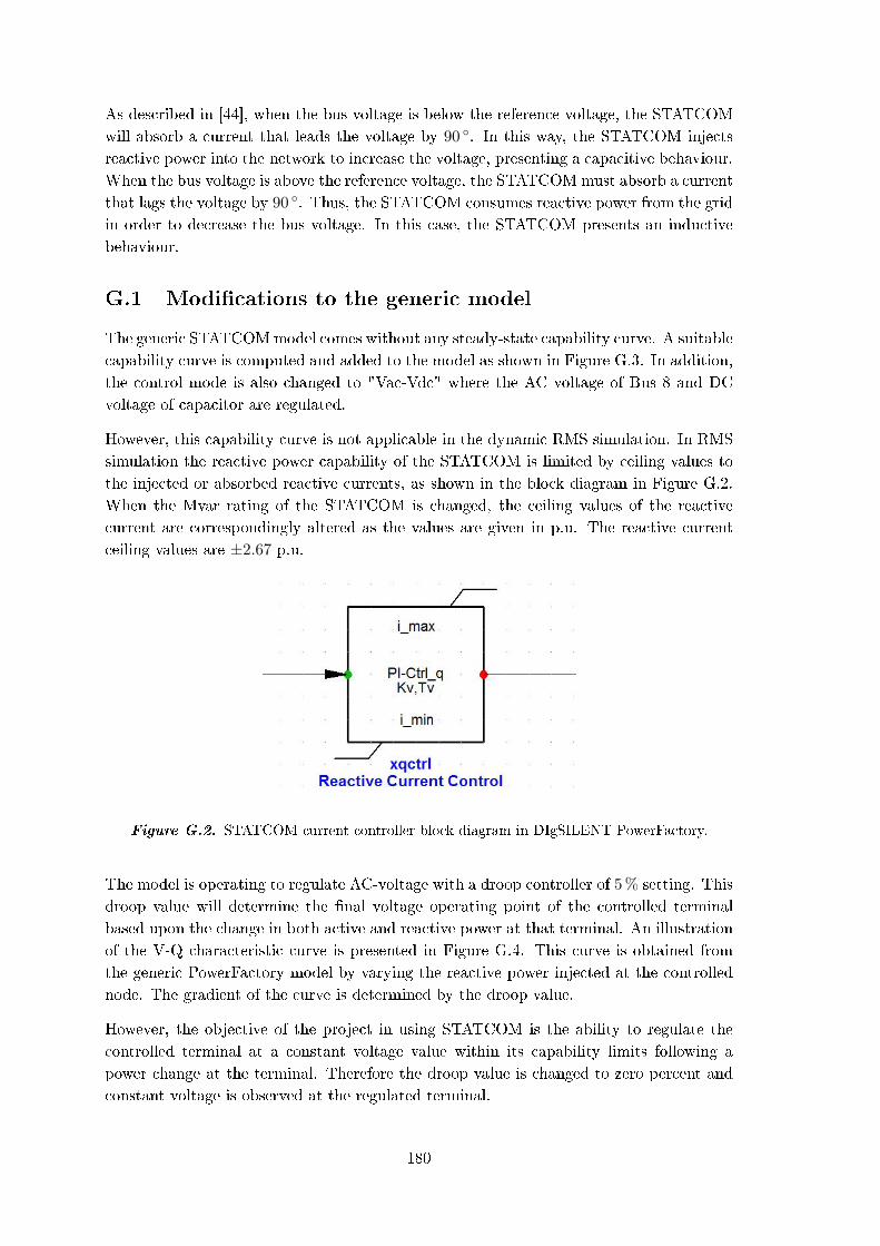
As described in [44], when the bus voltage is below the reference voltage, the STATCOM

will absorb a current that leads the voltage by 90 . In this way, the STATCOM injects

reactive power into the network to increase the voltage, presenting a capacitive behaviour.

When the bus voltage is above the reference voltage, the STATCOMmust absorb a current

that lags the voltage by 90 . Thus, the STATCOM consumes reactive power from the grid

in order to decrease the bus voltage. In this case, the STATCOM presents an inductive

behaviour.

G.1 Modications to the generic model

The generic STATCOMmodel comes without any steady-state capability curve. A suitable

capability curve is computed and added to the model as shown in Figure G.3. In addition,

the control mode is also changed to "Vac-Vdc" where the AC voltage of Bus 8 and DC

voltage of capacitor are regulated.

However, this capability curve is not applicable in the dynamic RMS simulation. In RMS

simulation the reactive power capability of the STATCOM is limited by ceiling values to

the injected or absorbed reactive currents, as shown in the block diagram in Figure G.2.

When the Mvar rating of the STATCOM is changed, the ceiling values of the reactive

current are correspondingly altered as the values are given in p.u. The reactive current

ceiling values are ±2.67 p.u.

Figure G.2. STATCOM current controller block diagram in DIgSILENT PowerFactory.

The model is operating to regulate AC-voltage with a droop controller of 5 % setting. This

droop value will determine the nal voltage operating point of the controlled terminal

based upon the change in both active and reactive power at that terminal. An illustration

of the V-Q characteristic curve is presented in Figure G.4. This curve is obtained from

the generic PowerFactory model by varying the reactive power injected at the controlled

node. The gradient of the curve is determined by the droop value.

However, the objective of the project in using STATCOM is the ability to regulate the

controlled terminal at a constant voltage value within its capability limits following a

power change at the terminal. Therefore the droop value is changed to zero percent and

constant voltage is observed at the regulated terminal.

180

Figure G.3. Screenshot of the load ow tab in the STATCOM model.

-20 -15 -10 -5 0 5 10 15 20

Injected reactive power, Qi [Mvar]

0.975

0.98

0.985

0.99

0.995

1

1.005

1.01

1.015

1.02

Bus

8 v

olta

ge in

p.u

.

Figure G.4. V-Q characteristic .

181

Additional case studies ofSR-switching and

STATCOM HThis appendix present additional study cases of SR-switching and STATCOM similar to

the one presented in Section 6.4.7.

Disturbance in Area G, observing Bus 12

Figure H.1 compares SR-switching and STATCOM for the disturbances in Area G, where

the voltage at Bus 12 is observed. In support of the results show in Figure 6.23, this

case reveal that the STATCOM is over-dimensioned in combination of SR-switching if it

placed directly in the weakened area. To benet from the combination, the capacity of the

STATCOM could be reduced or the STATCOM could be relocated to the area border (Bus

5). The presence of the STATCOM at either locations smoothens the voltage trajectory,

but the aforementioned problem of voltage spikes at the instant of SR-switching remains.

5 10 15 20 25 30

Time, t [s]

0.8

0.85

0.9

0.95

1

1.05

1.1

Bus

12

volta

ge in

p.u

.

Large-disturbance Case 1

SR-switching onlySTATCOM Bus 12 & 28STATCOM Bus 5 & 27No SR-sw. STATCOM 12 & 28No SR-sw. STATCOM 5 & 27

0 2 4 6 8 10 12 14 16 18

Time, t [s]

0.75

0.8

0.85

0.9

0.95

1

1.05

1.1

1.15

Bus

12

volta

ge in

p.u

.

Large-disturbance Case 2

SR-switching onlySTATCOM Bus 12 & 28STATCOM Bus 5 & 27No SR-sw. STATCOM 12 & 28No SR-sw. STATCOM 5 & 27

Figure H.1. Comparison of voltage trajectories at Bus 12 with STATCOMs in the network,

with and without SR-switching. Left: Large-disturbance Case 1. Right: Large-

disturbance Case 2.

Disturbance in Area A, observing Bus 3

Figure H.2 compares SR-switching and STATCOM for the disturbances in Area A, where

the voltage at Bus 3 is observed. A STATCOM is not placed directly in Area A as it was

dened as a strong area in the short-circuit analysis and by the Q,V -curves. The nearest

STATCOM is at Bus 5, when the area border STATCOM placement is used. Thus, the

most improved voltage trajectory at Bus 3 is observed when there is a STATCOM located

at Bus 3.

183

For both disturbance Case 4 and Case 5 it is shown that the STATCOM is unable to

supply sucient reactive power without the aid of the SR-switching. In the combination

of SR-switching and STATCOM the voltage trajectory is smooth and stabilizes quicker.

0 2 4 6 8 10 12 14 16 18 20

Time, t [s]

0.65

0.7

0.75

0.8

0.85

0.9

0.95

1

1.05

1.1

Bus

3 v

olta

ge in

p.u

.

Large-disturbance Case 4

SR-switching onlySTATCOM Bus 12 & 28STATCOM Bus 5 & 27No SR-sw. STATCOM 12 & 28No SR-sw. STATCOM 5 & 27

5 10 15 20 25 30

Time, t [s]

0.85

0.9

0.95

1

1.05

1.1

Bus

3 v

olta

ge in

p.u

.

Large-disturbance Case 5

SR-switching onlySTATCOM Bus 12 & 28STATCOM Bus 5 & 27No SR-sw. STATCOM 12 & 28No SR-sw. STATCOM 5 & 27

Figure H.2. Comparison of voltage trajectories at Bus 3 with STATCOMs in the network,

with and without SR-switching. Left: Large-disturbance Case 4. Right: Large-

disturbance Case 5.

Figure H.2(left) show that without SR-switching, disturbance Case 4 leads to transient

instability. Recalling Section 6.4.4, power angle oscillations are observed, but without the

STATCOMs the system nds a stable equilibrium. In other words, when STATCOMs

are included in the system model, Case 4 leads to transient instability unless the shunt

reactors are switched. It is highly likely that this result is due to limitations of the simple

STATCOM model used for this study. However, due to time constraints of the project

work presented in this thesis, this event is not investigated further. Though, caution

should be paid towards the behaviour of the STATCOM model in future work.

184

Utilizing Q,V-characteristicsfor SR-switching I

This appendix present the unsolved and very basic thoughts behind dQ/dV based SR-

switching. The purpose is to support the argument that further analysis of this concept

should be investigated in future work.

Recalling the Q,V -curves presented in Section 6.3. The gradients dQ/dV describes how

the voltage at a given bus reacts to changes in reactive power locally. Switching of SRs

is analogous to injecting reactive power by letting the cables supply Q, and thus move

in positive voltage direction on the Q,V -curve, as long as the system is operating above

critical level.

Thus, it is relevant to discuss if there exist a relation between the dQ/dV -sensitivities of

the network, and the necessary Qsw required to restore voltages in a large-disturbance

event. Hence, the question is if utilizing Q,V -characteristics is a possible method for

developing sequential switching schemes of SRs.

It is important to note that the Q,V -curves are produced for steady-state condition where

the topology of the network is intact. Thus, a dierence must be expected between the

voltage response to the injection of Qi in the steady-state and the electromechanical

transient. In the transient state, the Q,V -sensitivity is aected by topological changes

due line switching, loss of generation and interactions of AVR systems.

Using the data presented in Figures 6.7, 6.8 and 6.9, linearised ∆Q/∆V -slopes are dened

for three dierent voltage ranges. Figure I.1 show the basic concept of the linearisation.

For simplicity three ranges of voltage are dened, for which the ∆Q/∆V -slope are

specied. Table I.1 show the ∆Q/∆V for the three dierent areas in three dierent

voltage ranges.

Table I.1. Linearised ∆Q/∆V slopes based on Q,V -curves. The values indicate the necessary

Qi in Mvar to increase the voltage by 0.1 p.u.

∆Q/∆V [Mvar/0.1 p.u.]

Bus Area Vcrit < V < 0.8 0.8 < V < 0.9 0.9 < V < 1.0

3 A 242.42 714.29 1119.4

12 G 156.25 271.17 393.01

28 F 110.81 181.76 549.79

185

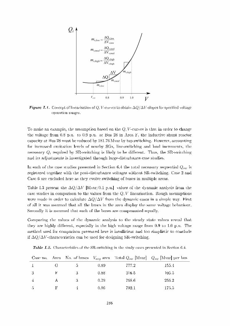
Qi

V0.90.8 1.0Vcrit

∆Qv,low∆Vv,low

∆Q∆V

mv,low

mv,med

mv,high

mv,low =

∆Qv,med∆Vv,med

mv,med =

∆Qv,high∆Vv,high

mv,high =

Figure I.1. Concept of linearisation ofQ,V -curves to obtain ∆Q/∆V -slopes for specied voltage

operation ranges.

To make an example, the assumption based on the Q,V -curves is that in order to change

the voltage from 0.8 p.u. to 0.9 p.u. at Bus 28 in Area F, the inductive shunt reactor

capacity at Bus 28 must be reduced by 181.76 Mvar by tap switching. However, accounting

for increased excitation levels of nearby SGs, line-switching and load increments, the

necessary Qi required by SR-switching is likely to be dierent. Thus, the SR-switching

and its adjustments is investigated through large-disturbance case studies.

In each of the case studies presented in Section 6.4 the total necessary sequential Qsw is

registered together with the post-disturbance voltages without SR-switching. Case 2 and

Case 6 are excluded here as they evolve switching of buses in multiple areas.

Table I.3 present the ∆Q/∆V [Mvar/0.1 p.u.] values of the dynamic analysis from the

case studies in comparison to the values from the Q,V linearisation. Rough assumptions

were made in order to calculate ∆Q/∆V from the dynamic cases in a simple way. First

of all it was assumed that all the buses in the area display the same voltage behaviour.

Secondly it is assumed that each of the buses are compensated equally.

Comparing the values of the dynamic analysis to the steady state values reveal that

they are highly dierent, especially in the high voltage range from 0.9 to 1.0 p.u. The

method used for comparison presented here is insucient and too simplistic to conclude

if ∆Q/∆V -characteristics can be used for designing SR-switching.

Table I.2. Characteristics of the SR-switching in the study cases presented in Section 6.4.

Case no. Area No. of buses Vavg area Total Qsw [Mvar] Qsw [Mvar] per bus

1 G 5 0.89 777.2 155.4

3 F 3 0.88 316.5 105.5

4 A 3 0.79 768.6 256.2

5 F 4 0.86 702.1 175.5

186

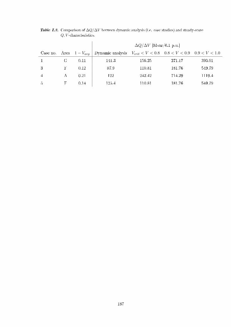
Table I.3. Comparison of ∆Q/∆V between dynamic analysis (i.e. case studies) and steady-state

Q,V -characteristics.

∆Q/∆V [Mvar/0.1 p.u.]

Case no. Area 1− Vavg Dynamic analysis Vcrit < V < 0.8 0.8 < V < 0.9 0.9 < V < 1.0

1 G 0.11 141.3 156.25 271.17 393.01

3 F 0.12 87.9 110.81 181.76 549.79

4 A 0.21 122 242.42 714.29 1119.4

5 F 0.14 125.4 110.81 181.76 549.79

187

CD content JThe CD contains the following:

Data and plots in Matlab File location

SMIB \Matlab scripts\ SMIB

9bus_voltage_stab \Matlab scripts\9-bus9bus_transient_stab \Matlab scripts\9-bus39bus_voltage_stab \Matlab scripts\39-bus39bus_transient_stab \Matlab scripts\39-bus

DIgSILENT PowerFactory models File location

SMIB_eqcable \Models

9-bus_eqcable \Models

39-bus_eqcable \Models

39-bus_STATCOM \Models

Misc File location

Report.pdf \Selected gures \Images