POWER SYSTEM FLEXIBILITY FOR THE ENERGY TRANSITION
76
POWER SYSTEM FLEXIBILITY FOR THE ENERGY TRANSITION PART II: IRENA FLEXTOOL METHODOLOGY November 2018 www.irena.org
Transcript of POWER SYSTEM FLEXIBILITY FOR THE ENERGY TRANSITION

POWER SYSTEM FLEXIBILITY FOR THE ENERGY TRANSITIONPART II: IRENA FLEXTOOL METHODOLOGY
November 2018
www.irena.org

Copyright © IRENA 2018
Unless otherwise stated, material in this publication may be freely used, shared, copied, reproduced, printed and/or
stored, provided that appropriate acknowledgement is given of IRENA as the source and copyright holder. Material in this
publication that is attributed to third parties may be subject to separate terms of use and restrictions, and appropriate
permissions from these third parties may need to be secured before any use of such material.
ISBN 978-92-9260-090-7
Citation: IRENA (2018), Power System Flexibility for the Energy Transition, Part 2: IRENA FlexTool methodology,
International Renewable Energy Agency, Abu Dhabi.
About IRENA
The International Renewable Energy Agency (IRENA) is an intergovernmental organisation that supports countries in their transition to a sustainable energy future and serves as the principal platform for international co-operation, a centre of excellence, and a repository of policy, technology, resource and financial knowledge on renewable energy. IRENA promotes the widespread adoption and sustainable use of all forms of renewable energy, including bioenergy, geothermal, hydropower, ocean, solar and wind energy, in the pursuit of sustainable development, energy access, energy security and low-carbon economic growth and prosperity.
Acknowledgements
This report benefited from the input of various experts, notably Debabrata Chattopadhyay (World Bank), Todd Levin (Argonne National Laboratory), Debra Lew (General Electric), Michael Milligan (consultant, ex-NREL), Simon Müller (IEA), Sakari Oksanen (consultant, ex-IRENA), Aidan Tuohy (EPRI) and Manuel Welsch (IAEA). Dolf Gielen and Asami Miketa (IRENA) also provided valuable input.
Contributing authors: Emanuele Taibi, Thomas Nikolakakis, Laura Gutierrez and Carlos Fernandez (IRENA) with Juha Kiviluoma, Tomi J. Lindroos and Simo Rissanen (VTT).
The report is available for download: www.irena.org/publications.
For further information or to provide feedback: [email protected]
Disclaimer
This publication and the material herein are provided “as is”. All reasonable precautions have been taken by IRENA to verify the reliability of the material in this publication. However, neither IRENA nor any of its officials, agents, data or other third-party content providers provides a warranty of any kind, either expressed or implied, and they accept no responsibility or liability for any consequence of use of the publication or material herein.
The information contained herein does not necessarily represent the views of the Members of IRENA. The mention of specific companies or certain projects or products does not imply that they are endorsed or recommended by IRENA in preference to others of a similar nature that are not mentioned. The designations employed and the presentation of material herein do not imply the expression of any opinion on the part of IRENA concerning the legal status of any region, country, territory, city or area or of its authorities, or concerning the delimitation of frontiers or boundaries.

3
CONTENTS
FIGURES ��������������������������������������������������������������������������������������������������������������������������������������������������� 5
TABLES �����������������������������������������������������������������������������������������������������������������������������������������������������6
ABBREVIATIONS ����������������������������������������������������������������������������������������������������������������������������������� 7
1 INTRODUCTION �������������������������������������������������������������������������������������������������������������������������������8
2 OVERVIEW OF EXISTING APPROACHES FOR FLEXIBILITY ASSESSMENT ���������������������9
3 OVERVIEW OF THE IRENA FLEXTOOL ������������������������������������������������������������������������������������15
4 USING THE IRENA FLEXTOOL ��������������������������������������������������������������������������������������������������� 18
4�1 Identifying flexibility needs and least-cost flexibility options ��������������������������������� 20
4�2 Studying a current system ���������������������������������������������������������������������������������������������������21
4�3 Representing more complex forms of generation and consumption ����������������������22
4�4 Using the FlexTool for other purposes �����������������������������������������������������������������������������22
5 IRENA FLEXTOOL MODEL DESCRIPTION ������������������������������������������������������������������������������23
5�1 Main modelling assumptions ����������������������������������������������������������������������������������������������25
5�2 Dimensions of the model �����������������������������������������������������������������������������������������������������26
5�3 Variables ����������������������������������������������������������������������������������������������������������������������������������27
5�4 Objective function �����������������������������������������������������������������������������������������������������������������28
5�5 Demand-supply balance ������������������������������������������������������������������������������������������������������28
5�6 Other constraints and auxiliary equations ����������������������������������������������������������������������29
5�7 Mathematical formulation ��������������������������������������������������������������������������������������������������� 31

POWER SYSTEM FLEXIBIL ITY FOR THE ENERGY TRANSITION4
6 IRENA FLEXTOOL INPUT DATA �����������������������������������������������������������������������������������������������32
6�1 Introduction ����������������������������������������������������������������������������������������������������������������������������32
6�2 Input data file �������������������������������������������������������������������������������������������������������������������������32
6�3 Input data structure ��������������������������������������������������������������������������������������������������������������32
6�4 Selection of time periods for the investment (and dispatch) model �����������������������37
7 IRENA FLEXTOOL RESULTS �������������������������������������������������������������������������������������������������������39
7�1 Flexibility needs, capabilities and violations ������������������������������������������������������������������39
7�2 Operational view �������������������������������������������������������������������������������������������������������������������47
7�3 Cost-effective flexibility �������������������������������������������������������������������������������������������������������47
7�4 Identifying and solving flexibility issues �������������������������������������������������������������������������52
8 INSIGHTS FROM CASE STUDIES ���������������������������������������������������������������������������������������������� 54
8�1 Introduction ��������������������������������������������������������������������������������������������������������������������������� 54
8�2 Engagement process and relevant stakeholders ����������������������������������������������������������55
8�3 Input data requirements ������������������������������������������������������������������������������������������������������55
8�4 IRENA FlexTool simulations for the case studies ����������������������������������������������������������57
8�5 Flexibility indicators used in the case studies ���������������������������������������������������������������57
8�6 Final outcomes of the case studies ����������������������������������������������������������������������������������59
8�7 Further work with the IRENA FlexTool �����������������������������������������������������������������������������59
REFERENCES ��������������������������������������������������������������������������������������������������������������������������������������� 60
APPENDIX I� TOOL VALIDATION WITH PLEXOS �������������������������������������������������������������������������62
APPENDIX II� MODEL EQUATIONS ������������������������������������������������������������������������������������������������� 68
APPENDIX III� USING THE TOOL FOR PLANNING A FUTURE SYSTEM WITH HIGH SHARES OF VARIABLE RENEWABLE ENERGY �����������������������������������������������������74

PART I I : IRENA FLEXTOOL METHODOLOGY 5
FIGURES
Figure 1: The IRENA FlexTool in the planning process 14
Figure 2: IRENA FlexTool workflow 15
Figure 3: Flowchart on how to use the IRENA FlexTool depending on the investment information 17
Figure 4: Overview of the modelling process in the IRENA FlexTool 18
Figure 5: The three alternative ways to run the optimisation for each scenario 19
Figure 6: An example of a common workflow with the IRENA FlexTool: identifying flexibility shortages and solving the least-cost flexibility options 20
Figure 7: Another example of a possible workflow with the IRENA FlexTool: studying the current electricity system under unexpected events, e� g�, poor water year, high natural gas price or broken interconnector 21
Figure 8: Overview of the tool input data (black font) and model variables, i� e�, outputs (red font) 23
Figure 9: Dispatch model solve time in minutes (right y-axis) for various problem sizes as expressed by the number of units and connections between the nodes (left y-axis) 24
Figure 10: Example of selection of representative periods for the IRENA FlexTool simulations based on demand and VRE penetration 38
Figure 11: Duration curve for energy demand and net load (lines) together with unit capacities (leftmost column for conventional capacity and rightmost for VRE and storage) 43
Figure 12: Ramp duration curve for demand and net load (change between two time periods) as well as upward ramping capabilities of units (leftmost column for conventional capacity and rightmost for VRE and storage) 43
Figure 13: Net load ramp with upward and downward one-hour ramping capabilities 44
Figure 14: Network diagram showing the installed capacity and peak demand per node (left side) and generation mix (right side) of the system used to present the results 45
Figure 15: Loss of load in different scenarios 45
Figure 16: Curtailment in different scenarios 46
Figure 17: Provision of reserves from different units calculated as full load hours 47
Figure 18: An example of generation to meet the demand + exports - imports 48
Figure 19: Full load hours of generation units in different scenarios 48
Figure 20: Total annualised costs in different scenarios 49

POWER SYSTEM FLEXIBIL ITY FOR THE ENERGY TRANSITION6
TABLES
Table 1: Overview of existing flexibility assessment approaches and their typical characteristics and limitations 11
Table 2: The sources and availability of existing flexibility assessment approaches 12
Table 3: Variables from the IRENA FlexTool model 27
Table 4: Sheet content descriptions for the input data workbooks 33
Table 5: Unit type parameters that can be defined for different unit type categories 35
Table 6: Summary of results from the IRENA FlexTool for four scenarios 41
Table 7: Summary of costs from the IRENA FlexTool for two example scenarios 50
Table 8: Relevant stakeholders participating in the engagement and data collection processes of the flexibility assessment 55
Table 9: Summary of data needed for a FlexTool case study 56
Table 10: Flexibility enablers of a specific power system 57
Table 11: Flexibility indicators assessed by the IRENA FlexTool 58
Table 12: Indicators to measure the remaining flexibility in the power system 58
Table 13: Characteristics of case studies 63
Table 14: Main differences between the IRENA FlexTool and PLEXOS running on MIP model 64
Table 15 Benchmarking results for case 1 65
Table 16 Benchmarking results for case 2 67
Table 17: Weighted average error of generation and cost 67
Figure 21: CO2 costs for the units in different scenarios 51
Figure 22: Investments in new capacity and the marginal value for additional capacity 51
Figure 23: Quick guide to how to check and solve grid issues in the IRENA FlexTool 53
Figure 24: Methodology followed to develop country case studies 54
Figure 25: Possible workflow for analysing investment scenarios for a target year 74

PART I I : IRENA FLEXTOOL METHODOLOGY 7
ABBREVIATIONSAC alternating current
AMPL a mathematical programming language
CAISO California Independent System Operator
cf capacity factor
Clp COIN-OR linear programming
CO₂ carbon dioxide
CSP concentrated solar power
csv comma-separated values
DC direct current
EDF Électricité de France
EPRI Electric Power Research Institute
ERCOT Electric Reliability Council of Texas
FAST2 Flexibility Assessment Tool 2
GIVAR Grid Integration of Variable Renewables
GLPK GNU Linear Programming Kit
GWh gigawatt-hour
IEA International Energy Agency
IRENA International Renewable Energy Agency
IRRE Insufficient Ramping Resource Expectation
kW kilowatt
kWh kilowatt-hour
LP linear programming
M USD millions of US dollars
MIP mixed integer programming
MW megawatt
MWh megawatt-hour
NASA National Aeronautics and Space Agency (United States)
NREL National Renewable Energy Laboratory (United States)
OPF optimal power flow
O&M operation and maintenance
p. u. unitary magnitude
PV photovoltaic
SNSP system non-synchronous penetration
TSO transmission system operator
TWh terawatt-hour
USD US dollar
VRE variable renewable energy

POWER SYSTEM FLEXIBIL ITY FOR THE ENERGY TRANSITION8
1 INTRODUCTION
The growth in variable renewable energy (VRE), notably wind and solar photovoltaics (PV), has focused efforts worldwide on the need for flexibility in electricity systems�
In Part 1 of this report has defined system flexibility as follows:
“Flexibility is the capability of a power system to cope with the variability and uncertainty that VRE generation introduces into the system in different time scales, from the very short to the long term, avoiding curtailment of VRE and reliably supplying all the demanded energy to customers.”
Following this definition and taking account of the various challenges encountered in practice, the International Renewable Energy Agency (IRENA) has developed a tool to assess the flexibility of any particular power system� This is the IRENA FlexTool�
While Part I provided an overview of flexibility challenges and solutions, Part 2 now aims to explain the methodology behind the FlexTool� Inevitably, this second part steers the discussion away from the policy level and more towards an audience of technical practitioners�
Within part 2, meanwhile, section 2 presents an overview of the existing approaches for flexibility assessment, and of the value added of the FlexTool� Sections 3 and 4 give a high-level overview of the IRENA FlexTool and its different uses� In Sections 5 to 7 the methodology, input data and result of the tool are presented from a technical perspective�
Finally, Section 8 offers key insights obtained from the first four countries where the FlexTool was applied� These cases can be useful for other IRENA members interested in applying the tool�
At the end of this report, Appendix I shows a comparison of the FlexTool with a widely used modelling tool that gives validity to the results obtained� Appendix II contains the mathematical formulation of the model, and Appendix III shows how the tool could be used for planning future systems with a high share of VRE�
Variable renewables introduce new levels of uncertainty into the power system at different time scales, from the very short to the very long term
nmacdonald
Stamp

PART I I : IRENA FLEXTOOL METHODOLOGY 9
2 OVERVIEW OF EXISTING APPROACHES FOR FLEXIBILITY ASSESSMENT
Existing flexibility assessment tools and methods are designed to serve different purposes ranging from visual comparisons to operational stochastics and planning with varying degrees of complexity� Simpler tools can be used to provide preliminary modelling for regions without extensive know-how and tools needed for detailed renewable integration studies, and to raise awareness and motivation for more detailed analysis, while more comprehensive tools can be an integral part of full-scale grid integration studies�
For example the NREL System Evaluation Tool (Milligan et al�, 2009) can act as a checklist for potential improvements in current practices, while the IRENA FlexTool can be used for more detailed analysis� In addition, each tool has a particular method for evaluating flexibility� The overall objective of these tools is the same, but the effort required to use them and the robustness of their results are different�
Based on complexity and level of detail, the existing approaches for flexibility assessment found in literature have been divided into three tiers:
• Tier 1: Tools with light data requirements, e� g�, no time series� These can be based on data about the generation portfolio, interconnections and other potential sources of flexibility and usually require expert judgement� A qualitative assessment can provide a quick comparison of different power systems and give guidance on where to start improving the system flexibility�
• Tier 2: Tools that calculate sufficiency of flexibility based on time series and more detailed unit data or based on a separate dispatch from an external tool, typically with calculations performed on a spreadsheet without full power system optimisation� Time series (e� g�, demand and variable generation, which should be synchronous with each other) are attained from historical data and/or meteorological sources and are converted for possible future situations� The tools are meant for screening potential issues (e� g�, curtailments and high ramps) as the share of variable generation increases� Power systems can be complex – due to, for example, interconnections, storage and links with other energy sectors – and consequently these tools use simplifications that try to capture the most important aspects from the perspective of flexibility�
• Tier 3: Tools based on dispatch models, possibly combined with generation planning models� Unit commitment and economic dispatch models are used extensively in power system operations and planning� Consequently they provide a solid foundation for analysing the sufficiency of flexibility� However, unit commitment tools are often sophisticated and require expert knowledge to be operated� They usually have been developed for other purposes than assessing flexibility, and therefore most of them require post-processing or other developments for flexibility analysis�

POWER SYSTEM FLEXIBIL ITY FOR THE ENERGY TRANSITION10
Tier 1 tools can be useful for increasing preliminary understanding of the possible challenges associated with the increase in variable generation in a particular power system� These tools also can highlight where possible solutions might be, but they will not provide much quantitative information� Tier 2 tools can indicate when more flexibility is likely to be required in order to avoid excessive curtailments� Tier 3 tools can be used either for planning operations in a system that already has a lot of variable generation (to prepare for situations where, for example, ramping capability could become scarce) or to support the planning of the expansion of a power system, including possible sources of flexibility�
Based on this classification, Table 1 provides a quick overview of several tools and methodologies that can be used for flexibility assessments, and presents typical characteristics and limitations of each� Table 2 provides information on the availability of each tool and methodology as well as references for more detailed descriptions of the models/tools�
Existing approaches range from tools with light data requirements to sophisticated tools based on dispatch models

PART I I : IRENA FLEXTOOL METHODOLOGY 11
Table 1: Overview of existing flexibility assessment approaches and their typical characteristics and limitations
Tier Approach Tool / Methodology
Typical characteristics Requirements and constraints
Tier 1
Expert comparison
NREL system evaluation (NREL)
Gives a framework for evaluating characteristics relevant from a flexibility perspective�
Requires expertise to score power systems from differ-ent flexibility perspectives� Not based on actual data�
Visual comparison
GIVAR (IEA), Flexibility Charts (Yasuda et al�, n� d�)
Presents a snapshot of the current situation with relevant informa-tion on generic flexibility� Fast to compare countries�
Based on a limited set of data� Can give only an overview�
Tier 2
Ramp evaluation
FAST2 (IEA), IRRE (Lannoye et al�, 2012)
Calculates system dispatch based on required net load (total load – VRE) and calculates required upward and downward ramping capabilities and resources for each hour or for longer periods� Reports insufficient ramping capabilities�
Dispatch using calculation rules based on either minimising cost or maximising flexibility� Focuses on ramping and reserves�
Operational stochastics
InFLEXion (EPRI)
Extension for a unit commitment or a dispatch tool� Uses results from the dispatch tool and histori-cal variability and uncertainty to assess potential flexibility short-falls in different situations�
Post-processing tool
Requires a separate unit commitment and dispatch model�
Flexibility check for/within planning tool
Flex Assessment (EDF), REFLEX (E3)
Assess within-hour flexibility needs in the planning phase� Pos-sibility to consider stochastics, operational constraints and ad-ditional reserves�
Pre-optimisation tool
Requires a separate planning and unit commitment model�
Tier 3
Reserve evaluation
FESTIV (NREL) Unit commitment, dispatch and reserve provision tool for scenarios with high levels of VRE� Can be used to explore different strategies to operate the system and the reserves� Focuses on relatively short time scales (seconds to day-ahead)�
High level of detail and consequently requires considerable expertise to be used effectively� Does not perform capacity expansion, only system operations�
Planning and operations
REFlex (NREL), RESOLVE (E3)
Optimises future dispatch and/or portfolios (capacity, storages, demand response) while considering operational constraints relevant from a flexibility perspective� RESOLVE also performs least-cost capacity expansion planning�
REFlex uses time slices where storage is handled with a valley-filling algorithm, which may result in inaccuracies� RESOLVE is a proprietary tool�
Planning and operations
IRENA FlexTool Optimises dispatch, investments or both� Can be used to explore whether the power system has sufficient flexibility and how to improve the flexibility of the system�
Requires generator, grid and time-series data� Linear optimisation only� Freely available from IRENA’s website�

POWER SYSTEM FLEXIBIL ITY FOR THE ENERGY TRANSITION12
Table 2: The sources and availability of existing flexibility assessment approaches
Tier Tool Report / paper Owner Public availability¹
Tier 1
NREL System Evaluation Tool
Milligan et al�, 2009 NREL Contact the author
GIVAR IEA, 2014 IEA Not available
Flexibility Charts Yasuda et al�, n�d Yasuda
et al� Contact the author
Tier 2
FAST2 IEA, 2014 IEA Contact the IEA
IRRE Lannoye et al�, 2012 Lannoye et al� Not available
InFLEXion Tuohy, 2016 EPRI EPRI (commercial)
REFLEX Hargreaves et al�, 2015 E3 E3 (not for sale)
Flex Assessment Silva et al�, n�d� EDF Not available
Tier 3
FESTIV Ela et al�, 2011 NREL Contact the author
REFlex Denholm and Margolis, 2007 NREL Proprietary
RESOLVE CAISO, 2016 E3 E3 (not for sale)
IRENA FlexTool This report IRENA IRENA (free)
1 When “contact the author” is stated, contacts are available in the original publication listed in the references.
The IRENA FlexTool was developed using the principles of Tier 3� It is an optimisation tool capable of solving the hourly (or sub-hourly if data are available) economic dispatch problem of a specific power system for one year� Until this point, there is no difference with any other tool in literature capable of solving an economic dispatch problem� However, the FlexTool adds value when compared with the other flexibility approaches because:
• Although it uses a typical economic dispatch formulation, the input data as well as the results are focused on power system flexibility (see Section 6 and Section 7)�
• The FlexTool is capable of solving a capacity expansion problem looking at a one-year horizon, which gives an overview of the most suitable flexibility solutions for a specific power system� None of the above-mentioned existing tools is capable of doing this�
• The FlexTool is the only publicly and freely available tool that performs capacity expansion and dispatch with a focus on power system flexibility�
Apart from this, the FlexTool was intended to be a detailed enough but simplified approach; therefore some simplifications had to be made:
PART I I : IRENA FLEXTOOL METHODOLOGY 13
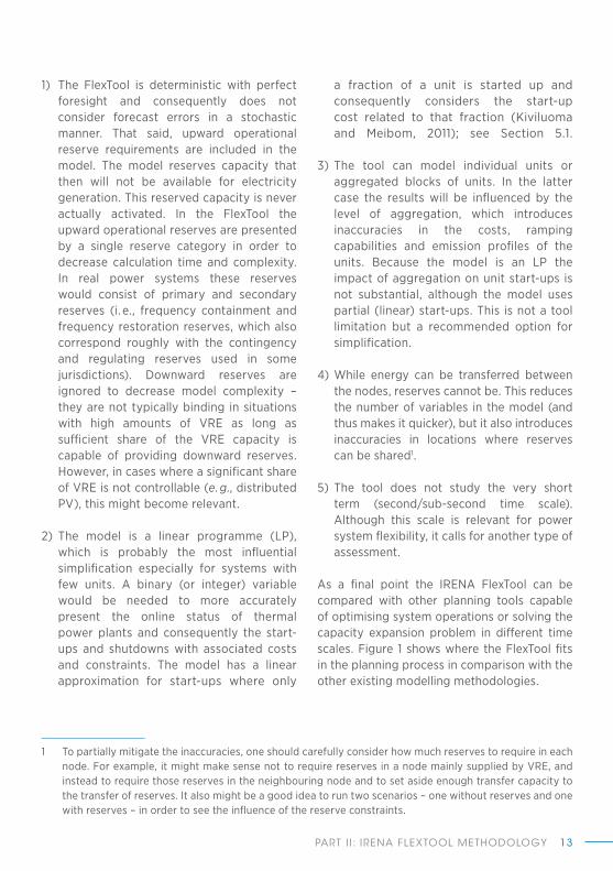
1) The FlexTool is deterministic with perfect foresight and consequently does not consider forecast errors in a stochastic manner� That said, upward operational reserve requirements are included in the model� The model reserves capacity that then will not be available for electricity generation� This reserved capacity is never actually activated� In the FlexTool the upward operational reserves are presented by a single reserve category in order to decrease calculation time and complexity� In real power systems these reserves would consist of primary and secondary reserves (i� e�, frequency containment and frequency restoration reserves, which also correspond roughly with the contingency and regulating reserves used in some jurisdictions)� Downward reserves are ignored to decrease model complexity – they are not typically binding in situations with high amounts of VRE as long as sufficient share of the VRE capacity is capable of providing downward reserves� However, in cases where a significant share of VRE is not controllable (e� g�, distributed PV), this might become relevant�
2) The model is a linear programme (LP), which is probably the most influential simplification especially for systems with few units� A binary (or integer) variable would be needed to more accurately present the online status of thermal power plants and consequently the start-ups and shutdowns with associated costs and constraints� The model has a linear approximation for start-ups where only
1 To partially mitigate the inaccuracies, one should carefully consider how much reserves to require in each node� For example, it might make sense not to require reserves in a node mainly supplied by VRE, and instead to require those reserves in the neighbouring node and to set aside enough transfer capacity to the transfer of reserves� It also might be a good idea to run two scenarios – one without reserves and one with reserves – in order to see the influence of the reserve constraints�
a fraction of a unit is started up and consequently considers the start-up cost related to that fraction (Kiviluoma and Meibom, 2011); see Section 5�1�
3) The tool can model individual units or aggregated blocks of units� In the latter case the results will be influenced by the level of aggregation, which introduces inaccuracies in the costs, ramping capabilities and emission profiles of the units� Because the model is an LP the impact of aggregation on unit start-ups is not substantial, although the model uses partial (linear) start-ups� This is not a tool limitation but a recommended option for simplification�
4) While energy can be transferred between the nodes, reserves cannot be� This reduces the number of variables in the model (and thus makes it quicker), but it also introduces inaccuracies in locations where reserves can be shared1�
5) The tool does not study the very short term (second/sub-second time scale)� Although this scale is relevant for power system flexibility, it calls for another type of assessment�
As a final point the IRENA FlexTool can be compared with other planning tools capable of optimising system operations or solving the capacity expansion problem in different time scales� Figure 1 shows where the FlexTool fits in the planning process in comparison with the other existing modelling methodologies�

POWER SYSTEM FLEXIBIL ITY FOR THE ENERGY TRANSITION14
Figure 1: The IRENA FlexTool in the planning process
FlexTool in the planning process
Optimal Capacity Expansion
System OperationGrid Studies
(Power Factory1, PSS/E2)
1 Second 1 Hour 1 Year 10 Years 50 Years
Time Horizon Analysed
FlexTool Dispatch
FlexTool Expansion
Dispatch Models (PLEXOS-ST3, SDDP4)
Capacity Expansion Models(PLEXOS-LT3, Opt-Gen4)
Energy Planning Models (Message5, MARKAL/TIMES6)
1Copyrighted by DIgSILENT GmbH2Copyrighted by Siemens PTI3Copyrighted by Drayton Analytics Pty Ltd, Australia and Energy Exemplar Pty Ltd, Australia4Developed by PSR5Developed by the International Atomic Energy Agency (IAEA)6Developed by the International Energy Agency (IEA)
The IRENA FlexTool dispatch and investment horizon ranges from less than a year to two years2, and within this horizon the tool can optimise both system operations and capacity expansion using an LP solver� Commercial modelling tools can also solve this problem using more powerful solvers with mixed integer programming (MIP); however, depending on the complexity of the problem, differences between solving an LP or an MIP might not be so high�
The FlexTool was benchmarked comparing it with a commercial modelling tool that uses MIP and a commercial solver, and the results showed no major differences between the two models (see Appendix I)� This does not mean that the FlexTool performs equal
2 The IRENA FlexTool could simulate more years; however, this tool solves the problem in only one step, and when analysing more than two years in a row the solving time could be high and it could make sense to use any other of the presented tools� Furthermore, it is beyond the scope of the tool to look at long time horizons�
to or better than commercial modelling tools, but it validates the results that the FlexTool is producing and demonstrates that when the input data are sufficiently aggregated, the benefit of using more complex methodologies and tools is limited�
The clear advantage of the FlexTool is that it is open source, free and comparably easy to use, requiring less input data than is typical when modelling every single power plant with its specific technical characteristics at a high level of disaggregation� Based on this, the FlexTool can be a valuable addition to the power system planning toolkit, between long-term investment models and short-term operational and network models�

PART I I : IRENA FLEXTOOL METHODOLOGY 15
3 OVERVIEW OF THE IRENA FLEXTOOL
As already discussed, the IRENA FlexTool is capable, on the one hand, of analysing system operations using a time step that represents real-world challenges (an hour or less in the case of VRE variability)� On the other hand it can help to identify a least-cost mix of flexibility options for a given power system that might be facing insufficient flexibility at some points in time during operations�
The FlexTool was designed to have an accessible (i� e�, Microsoft Excel) interface, to encourage use by a broad range of stakeholders and presenting results in a concise, visual and informative way� It is an optimisation tool that has abilities to perform 1) long-term least-cost capacity expansion analysis and 2) short-term dispatch simulations� The main goal of the
model is to identify flexibility gaps in the short term and to explore optimal investments that support system flexibility in the long term�
The tool incorporates enough mathematical complexity to address important aspects of system flexibility while at the same time is less complex than advanced commercial packages designed for use by utilities, consulting firms and other institutions/organisations to address complex technical questions� The tool can model systems of any size, as long as input data are sufficiently aggregated (e� g�, generation by technology and fuel, not by power plant, and dividing the grid into a few regions rather than hundreds or thousands of nodes)� A simplified workflow of the tool is shown in Figure 2�
Figure 2: IRENA FlexTool workflow
Inputs:
• Generation mix
• Demand
• VRE profiles
• Scenarios
• Reserve requirements
• Investment candidates
• …
Outputs:
IRENAFlexTool
3.0
GW
2.5
2.0
1.5
1.0
0.5
0.0
-0.5

POWER SYSTEM FLEXIBIL ITY FOR THE ENERGY TRANSITION16
The FlexTool can perform the optimal scheduling of power system operations using economic dispatch with an option to optimise the investment into various flexibility sources and other technologies� The investment phase does not consider plant retirements� Existing investment planning (capacity expansion) and operational scheduling (i� e�, dispatch) tools typically require considerable experience to be operated, but the FlexTool is designed to be easier to use for less-expert users� It relies on a simplified Microsoft Excel interface with partially pre-filled data sets� The optimisation is performed using open-source software�
In comparison to generation expansion tools, where flexibility constraints are generally omitted or, when considered, are frequently limited to the flexibility from thermal generators (Poncelet et al�, 2018) the value added of a dispatch-focused tool like the FlexTool is in the explicit focus on flexibility constraints and consideration of all possible sources of flexibility in the investment phase (e� g�, going beyond more flexible generation, transmission expansion and storage to include sector coupling) aimed at addressing flexibility gaps, including coupling with heat and gas grids� This is necessary to avoid overestimation of integration challenges in high-VRE scenarios as a consequence of limiting the sources of flexibility for the power system to thermal generation only (Poncelet et al�, 2018)�
The FlexTool can be used in various ways as it can perform both an operational optimisation and an investment optimisation of the energy system� Flexibility issues are best revealed at the operational level, but often their mitigation requires investments in new assets� Therefore
a good flexibility tool needs both capabilities� The user can choose whether the portfolios are decided by the user or whether the planning of the investments is optimised by the model� Investments in the FlexTool can take place not only because of lack of flexibility but also due to economics, as it is also a suitable tool to solve a capacity expansion problem and to invest, for instance, in additional VRE (see Appendix III)�
When the portfolios are given by the user, the FlexTool performs a least-cost economic dispatch optimisation based on the provided time series (typically one year of hourly data)� When the portfolio is defined by enabling the model’s investment planning option, the investments are optimised typically using representative time periods in hourly resolution (see Section 6�4)� In either case, the dispatch optimisation is subsequently applied to detect if there is any issue with flexibility�
When the portfolios are given by the user, based on the existing or projected power system, this step explores any critical issues that are related to flexibility within the given system� If issues are detected in this step, an investment optimisation can be run to identify possible remedies for these flexibility issues� In this step the FlexTool will solve a capacity expansion problem and then perform a dispatch optimisation with the new investments, in order to reveal any remaining issues that the investment phase was not able to consider (it simplifies certain aspects, as explained later)� These two suggested ways of using the FlexTool are represented in Figure 3, and a flowchart on how to identify and solve flexibility issues using the tool is shown in Figure 23 in Section 7�4�

PART I I : IRENA FLEXTOOL METHODOLOGY 17
The tool presents the results highlighting possible operational problems arising from insufficient flexibility as well as costs related to the investments and operations� In order to be easy to use, the tool simplifies some aspects of power system planning and operations that are required for safe and secure operation of power systems with high levels of VRE (most notably those aspects that are concerned with the stability control of the power system as well as the changes in the operational scheduling that would be used to manage the increasing forecast errors; see more detailed description in Section 5� A more thorough approach, which the FlexTool can be a part of, is described by the IEA Wind Task 25 report on the recommended practices for integration studies (IEA Wind Task 25, 2018) and also by the IRENA report Planning for the renewable future (IRENA, 2017)�
The IRENA FlexTool has been developed with the VTT Technical Research Centre of Finland Ltd (VTT, 2018) and as of 2018 is the only publicly and freely available tool that performs capacity expansion and dispatch with a focus on power system flexibility�
Figure 3: Flowchart on how to use the IRENA FlexTool depending on the investment information
Initial inputdata
Investmentsportfoliogiven?
Flexibilityassessment
Any flexibility
issue?
End of theanalysis
Redefineinvestmentcandidatesand changesimulation
periods
YesYes
No
No Optimalinvestments
FlexTool runin dispatch
mode
FlexTool runin investment
mode
The tool highlights possible operational problems and costs arising from insufficient flexibility

POWER SYSTEM FLEXIBIL ITY FOR THE ENERGY TRANSITION18
4 USING THE IRENA FLEXTOOL
Figure 4 gives an overview of the modelling process using the IRENA FlexTool� First, the user needs to input all necessary technology and cost data as well as time series into an input data workbook� Without these data, the behaviour of the system is not possible to model� The input data workbook defines the base scenario� The workbook indicates if there are obvious inconsistencies or deficiencies in the given data through data validation rules in
the input data workbooks� Then, in the FlexTool master workbook, additional scenarios can be defined� For example the tool can analyse different scenarios where the VRE generation capacity is high and where the VRE might cause flexibility issues� Multiple scenarios can then be run automatically, and the results will be available automatically for comparison in the results workbook�
Original data sources
IRENA FlexTool
Energy system model and an open-source solver
Scenariodata
Scenarioresults
Input data workbooksSystem data Technical data Time series
Master workbookSensitivity scenarios General settings Run the tool
Results workbook Flexibility needs Flexibility solutions Dispatch and costs
Figure 4: Overview of the modelling process in the IRENA FlexTool

PART I I : IRENA FLEXTOOL METHODOLOGY 19
The user also decides whether to use the dispatch optimisation alone (Alternative 1 in Figure 5) or to activate the investment planning module with or without the dispatch mode (Alternatives 2 and 3 in Figure 5)� The mode can be selected separately for each scenario� The investment mode optimises the investments and schedules all units, but it does not consider operational reserves, minimum loads or unit start-ups while it can use a capacity margin� The investment mode can use a reduced time-series set in order to reduce the computational burden�
After the investments have been optimised, the tool can re-optimise the full dispatch with all the constraints and the time series selected for the dispatch mode (Alternative 2 in Figure 5)� This can reveal issues not visible in the investment mode due to the additional constraints and possibly better representation of time� With
the investment optimisation activated, the tool can optimise additional investments in those flexibility options that have been included in the input data� Alternative 3 in Figure 5 would not be suitable for flexibility assessment, since it would not include all the operational constraints available in the FlexTool�
The tool then creates a results workbook to be interpreted by the user� The results workbook will highlight the main results and possible flexibility issues in a summary sheet (curtailment of VRE, loss of load due to insufficient peak capacity, loss of load due to insufficient ramping capability, reserves inadequacy as well as capacity inadequacy in the investment mode)� The issues can then be examined more closely using more detailed results spread out over several sheets�
Figure 5: The three alternative ways to run the optimisation for each scenario
Investment mode Dispatch mode
Dispatch mode1)
2)
3) Investment mode

POWER SYSTEM FLEXIBIL ITY FOR THE ENERGY TRANSITION20
The FlexTool can be used to analyse multiple scenarios� First the user defines a baseline data set, which serves as the base scenario� Then each new scenario is defined by making changes to the original base scenario (these changes can affect parameters related to either investments or operations)� In this way the user can easily perform sensitivity analysis on any parameter in the input data (e� g�, the maximum share of non-synchronous generation or reserve requirements)�
The results may show whether or not a power system has sufficient flexibility to cope with a high share of variable power generation� If not, then the user can investigate what has caused the problems by interpreting the graphs and values in the results workbook� The tool can then be used to search for reasonable sources of flexibility using the investment mode and also by manually including new sources of flexibility after the problems have been identified� To better illustrate, the three examples below explain various ways to use the tool3�
3 Appendix III explains how to use the IRENA FlexTool for planning, although this is not the primary purpose of the tool�
4.1 IDENTIFYING FLEXIBILITY NEEDS AND LEAST-COST FLEXIBILITY OPTIONS
Figure 6 provides a practical example of how to perform a flexibility assessment with the tool� The user defines a set of new input data, e� g�, expected or planned capacity mix for 2030, and runs the model for dispatch optimisation (i� e�, disabling new investments from the model run)� The model outputs all variables into the Excel results workbook, but the user can focus on the flexibility shortages (e� g�, unusual amount of VRE curtailment or loss of load), which are highlighted on the first sheet of the results workbook� The last step would be to make an alternative scenario, which has the same input data but the user allows the model to invest in new capacity (flexibility sources, i� e�, generation, storage or transmission)�
Comparing the results between these two runs, the user obtains, for example, least-cost flexibility solutions and capacity mix (additional capacity, additional interconnectors, additional storage)�
1. Input 2. Run the model
3. Results 4. Alternative run
• Estimated generation mix in a future scenario
• Identify flexibility shortages• Check if any other issues
• Run dispatch• New investments disabled
• Same input data, allow investments• Get least-cost flexibility solutions
Figure 6: An example of a common workflow with the IRENA FlexTool: identifying flexibility shortages and solving the least-cost flexibility options

PART I I : IRENA FLEXTOOL METHODOLOGY 21
The last step also could be replaced with a manual exploration of different options to mitigate the flexibility issues� For example, if there is a loss of load due to a shortage of generation capacity, the user can test different options to increase capacity in the power system using new generators, transmission lines or demand response and see how those impact the flexibility shortages and the total system costs� If the reason for the shortage is in the ramping capability of existing units (highlighted in the results), then the user can compare, for example, improving the ramping rate of existing units and building new, more flexible units� If there is too much curtailment of VRE, then the user could compare, for example, new transmission lines, storage and increasing the flexibility of electricity demand�
4.2 STUDYING A CURRENT SYSTEM
Figure 7 shows another example where the tool is used to study the current electricity system under an unexpected event, such as a poor hydro inflow year, high natural gas prices or an unavailable interconnector� In these runs, the user needs to first input the current electricity system, run the operational model and check the results� Once the scenario for a normal year works in the expected manner, the user can proceed to alternative scenarios – for example, decrease the amount of inflow to simulate a poor hydro inflow year, increase electricity demand, assume retirement of some units or try a low wind year�
Figure 7: Another example of a possible workflow with the IRENA FlexTool: studying the current electricity system under unexpected events, e. g., poor water year, high natural gas price or broken interconnector
1. Input 2. Run the model
3. Results 4. Alternative run
• Current electricity system
• Model run for normal year with current system• Check if any issues
• Run dispatch• New investments disabled
• Decrease water inflow to simulate poor water year• Run new dispatch and check cost increase + if enough electricity + if enough flexibility

POWER SYSTEM FLEXIBIL ITY FOR THE ENERGY TRANSITION22
From the new model run, the user would get a full set of results about, for example, the loss of load situations, lack of ramping capability and how the total system costs change� These are examples of issues that might be caused by the alternative scenario that stresses the system� The results can show where the problems might take place, and the tool could then be used to also find solutions for the possible problems�
A similar method can be applied to study future electricity systems, and it can be combined with investment optimisation to get least-cost flexibility solutions if so required�
4.3 REPRESENTING MORE COMPLEX FORMS OF GENERATION AND CONSUMPTION
The tool can represent more complex processes for electricity generation and consumption – including other energy sectors� This can be achieved by defining separate energy grids for the processes to be described� Some examples for these are in the provided input files: electric vehicles (EVs), simple demand response, a concentrated solar power (CSP) plant with internal heat storage, and a district heating grid� The inclusion of additional features in the model increases the problem size and may require either more computing power/memory or a smaller-size system, especially when performing investment optimisation�
,
Other energy sectors can be described in the same way as the power grid: units are connected to the nodes, and the energy grid consists of connected nodes� Transfer of energy between the nodes within the new energy grid works the same way as within the power grid (using net transfers and ignoring the electromagnetic characteristics of the power grid)� In addition, conversion units can convert energy from one grid to another� For instance, a heat pump connects the electricity grid to the heat grid, a hydrogen electrolyser connects the electricity grid to a gas grid, and a CSP generator connects a thermal grid to the electricity grid�
4.4 USING THE FLEXTOOL FOR OTHER PURPOSES
The main goal of the IRENA FlexTool is to assess the flexibility in specific power systems and to propose least-cost flexible solutions looking at one specific year� Although results are processed in a way that flexibility-related information is clearly displayed, the FlexTool, with some minor modifications, can be used as a power system modelling tool for other purposes� For instance, the FlexTool could be used to analyse the system operation, get the optimal dispatch and revenues of specific technologies, calculate the integration costs of VRE or plan a future system with high shares of VRE (see Appendix III)�

PART I I : IRENA FLEXTOOL METHODOLOGY 23
5 IRENA FLEXTOOL MODEL DESCRIPTION
4 The GNU MathProg Language is a subset of the AMPL programming language and is intended for describing linear mathematical programming models (Fourer et al�, 1990)�
The IRENA FlexTool model minimises the costs of operating a power system or a more general energy system� The tool can be used to assess multiple scenarios with different assumptions related to generation capacities, technological constraints, emission costs, etc� It has an option to perform investment optimisation into flexibility options, including generation and storage units as well as transmission lines� The model uses linear programming and is written in GNU MathProg4� Figure 8 provides an
overview of the tool’s input data and structure and describes the possible linkages to other energy grids, such as the heating grid, or other end-use sectors, which can be important flexibility sources�
The model includes a set of mathematical constraints that simulate the real technical constraints of power systems� These constraints include energy balance, reserve requirements, ramping constraints, minimum
Grid (power)
Time series Prices
Node
Demand time series
Generation
Transfer
Node 2
Node 3Import/export
time series
charge
HeatNode
Sector coupling (e.g., V2G)
Convert
State
Fuel use Online Start-up Reserve
Invest
Invest Invest
GasNode
EVNode
Figure 8: Overview of the tool input data (black font) and model variables, i. e., outputs (red font)

POWER SYSTEM FLEXIBIL ITY FOR THE ENERGY TRANSITION24
load constraints, transfer and conversion constraints, and a constraint on the maximum share of non-synchronous generation/imports�
The scenarios are solved with an open-source solver5 (both GLPK and COIN-OR Clp are included in the assessment package – Clp is likely to be considerably faster)� The solver minimises total system costs (including operational scheduling and optional investments in flexibility options) while respecting all constraints (as defined later in Sections 5�5 and 5�6)�
The FlexTool is capable of optimising generation, transmission and storage planning and a full year of hourly (or sub-hourly) operations� Since the model optimises everything at once, the problem can become too large to solve, especially when investment variables are included in the model�
5 A commercial problem solver such as CPLEX could also be used if the MathProg problem were adjusted to be solvable by such platforms�
The solving time is more or less linearly dependent on the problem size, as indicated by Figure 9 (using a 64-bit Intel i5-5400 central processing unit at 2�3 gigahertz and 8 gigabytes of memory)� Computer memory also can become an issue for larger problems� Some of the constraints (e� g�, reserves, minimum loads) can be easily relaxed so that larger system sizes can be solved with less computational effort�
In the following sub-sections, the model sets and variables are introduced, and the model equations are briefly described� Equations are fully formulated in the FlexTool model file (written in GNU MathProg), and Appendix II of this document contains the equations in a mathematical form�
0
20
40
60
80
100
120
0
20
40
60
80
100
120
140
160
Num
ber
of u
nits
/con
nect
ions
Run
tim
e (m
inut
es)
2016 hours
8760 hours
Units
Connections
5 nodes 10 nodes 15 nodes 15 nodes (more connections)
Figure 9: Dispatch model solve time in minutes (right y-axis) for various problem sizes as expressed by the number of units and connections between the nodes (left y-axis)

PART I I : IRENA FLEXTOOL METHODOLOGY 25
5.1 MAIN MODELLING ASSUMPTIONS
Operational reserves
The operational reserve can be set two ways� Both can be active, in which case both requirements have to be met at all times� In the first approach, operational reserve requirements in the model can depend on the share of wind and solar generation (reserve requirements are calculated as a fixed share of VRE generation in each time step, called dynamic reserve in the FlexTool)� In the second approach, operational reserve requirements can be set using time series, which allows for the use of constant reserve requirement or for establishing a more refined correlation between the reserve requirements and the VRE generation using external calculations or tools�
These two ways to set reserve requirements are independent constraints in the tool� This means that the user can use one approach, both or neither� If both reserve requirements are on at the same time, the tool checks which is higher in each time step and satisfies the higher one� If both reserve categories are switched off, the model operates without reserve constraints�
Note that the reserve requirement used in the FlexTool does not refer to tertiary reserves, but refers specifically to the reserve requirement for balancing variability and correcting forecasting error within the model time step�
Minimum stable level and start-up costs
As already mentioned, the FlexTool uses linear programming to solve the problem and therefore does not consider binary variables that would be required to model some flexibility parameters such as minimum stable
levels or start-up costs� However, the FlexTool considers a linear approximation similar to the one in Kiviluoma and Meibom (2011) to model these parameters� For this purpose the model includes an online variable, which represents the amount of power that is online per unit type� This variable includes not only generation but also upward reserve provision and curtailment�
Using this online variable, the minimum stable level constraint establishes that the total generation of a unit has to be greater than a user-specified fraction multiplied by the online variable� For instance, if we have 100 megawatts (MW) of coal online, with a minimum stable level of 40 %, coal has to generate at least 40 MW and can provide up to 60 MW of upward reserves�
To model start-up costs the approach is similar� Instead of starting up a bulk unit, as would happen in a mixed integer programme (MIP), the FlexTool starts up a fraction of a unit by using the variations in the online variable� Start-up costs are then applied only to this fraction� For instance, if at the first time step there is 100 MW of coal online and in the second time step there is 200 MW online, start-up costs will be applied to the additional 100 MW that was started�
Transmission network
In literature there are different approaches to model the transmission network� The most complete, but also the most complex, one would be modelling a full alternating current optimal power flow (AC-OPF)� However, this problem would contain non-linearities that would require techniques such as lagrangian relaxation or dynamic programming (Fu et al�, 2005) and is beyond the scope of the FlexTool� A common approach to simplify the AC power flow is the direct current optimal power flow

POWER SYSTEM FLEXIBIL ITY FOR THE ENERGY TRANSITION26
(DC-OPF), which linearises all the previous equations and considers only the real part of the power flow (active power) (Stott et al�, 2009)� This approach would be feasible to implement in the FlexTool; however, it would increase computational time and require some technical data (e� g�, resistance, reactance) that generally are not easy to access�
The FlexTool simplifies the DC-OPF and models the transmission network using a Transport Model6� This approach considers transmission lines between nodes as “pipelines” that can transfer a user-defined maximum power� With this approach all transmission lines have a controllable flow, and a flow variation in one line will not affect the others� Apart from this, line losses in the FlexTool are considered as linear, calculated as a user-defined fraction of the power flow� The FlexTool also differentiates between AC lines and DC lines by constraining the maximum system non-synchronous penetration (SNSP)�
5.2 DIMENSIONS OF THE MODEL
Sets are fundamental building blocks in any mathematical model, and they form the dimensions (time, space, etc�) of the model� Sets are used to define the scope of the model and the applicability of different equations in the model� In addition, the model uses subsets and multidimensional sets that define the confines of particular costs and constraints in the model (e� g�, fuel costs apply only to units that use fuel)� These are documented in the model description file�
6 The transport problem is a common optimisation problem in operations research� It consists of obtaining the least-cost plan to distribute goods or supplies from multiple origins to multiple destinations� In this case the goods to distribute are megawatts of electricity�
The four basic sets of the FlexTool model are:
• Grid (g). An energy grid, where energy of particular form can be generated, consumed and transferred (e� g�, electricity grid, gas grid, heat grid)�
• Node (n). A node in the energy grid aggregates generation and consumption of energy� Energy can be transferred between nodes in the same energy grid�
• Unit (u). Units represent devices that can generate energy from an exogenous source (e� g�, electricity from coal in a condensing coal power plant), reduce the consumption of energy that is included in the energy demand time series (price-sensitive demand response), increase the consumption of energy (for this, the unit type must define an “eff charge” parameter), store energy or convert energy from one energy form to another (e� g�, from power to heat)�
• Time (t). The modelled time span is divided into connected time periods� Time set represents all the available time periods in the model (based on input data), and a subset, which also can be equal to the full set, called time_in_use, defines the time periods actually in use�
FlexTool outputs can be time dependent and can be extracted per node, per unit or even per grid
PART I I : IRENA FLEXTOOL METHODOLOGY 27
5.3 VARIABLES
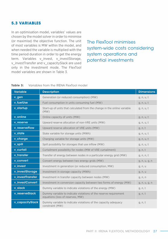
In an optimisation model, variables’ values are chosen by the model solver in order to minimise (or maximise) the objective function� The unit of most variables is MW within the model, and when needed the variable is multiplied with the time period duration in order to get the energy term� Variables v_invest, v_investStorage, v_investTransfer and v_capacitySlack are used only in the investment mode� The FlexTool model variables are shown in Table 3�
Table 3: Variables from the IRENA FlexTool model
Variable Description Dimensions
v_gen Generation (or reduced consumption) (MW) g, n, u, t
v_fuelUse Fuel consumption in units consuming fuel (MW) g, n, u, t
v_startup Start-up of units that calculated from the change in the online variable (MW)
g, n, u, t
v_online Online capacity of units (MW) g, n, u, t
v_reserve Upward reserve allocation of non-VRE units (MW) g, n, u, t
v_reserveFlow Upward reserve allocation of VRE units (MW) g, n, t
v_state State variable for storage units (MWh) g, n, u, t
v_charge Charging variable for storage units (MW) g, n, u, t
v_spill Spill possibility for storages that use inflow (MW) g, n, u, t
v_curtail Curtailment possibility for nodes (MW of VRE curtailment) g, n, t
v_transfer Transfer of energy between nodes in a particular energy grid (MW) g, n, n, t
v_convert Convert energy between two energy grids (MW) g, n, u, g, n
v_invest Investment in generation (or reduced consumption, MW) g, n, u
v_investStorage Investment in storage capacity (MWh) g, n, u
v_investTransfer Investment in transfer capacity between nodes (MW) g, n, n
v_investConvert Investment in conversion capacity between two forms of energy (MW) g, n, u, g, n
v_slack Dummy variable to indicate violations of the energy (MW) g, n, t
v_reserveSlack Dummy variable to indicate violations of the reserve requirement equations (loss of reserves, MW)
g, n, t
v_capacitySlack Dummy variable to indicate violations of the capacity adequacy constraint (MW)
g, n, t
The FlexTool minimises system-wide costs considering system operations and potential investments

POWER SYSTEM FLEXIBIL ITY FOR THE ENERGY TRANSITION28
5.4 OBJECTIVE FUNCTION
The model minimises the costs tabulated in the objective function (see Appendix II for the exact formulation)� These costs for the operational model are:
• fixed operation and maintenance (O&M) costs of units
• variable O&M costs of units• fuel costs of units• carbon dioxide (CO2) emission costs• start-up costs (using linear, i� e�, partial,
version of unit start-ups; compared in Kiviluoma and Meibom (2011))
• penalty cost for using v_slack variable (loss of load)
• penalty cost for using v_reserveSlack variable (insufficient upward reserves)
• penalty cost for using v_capacitySlack variable (insufficient capacity margin)
• penalty cost for using v_curtail variable (curtailment of VRE)�
If run in the investment mode, the model sees in addition to the above production costs also the investment costs (as annuities):
• unit investment costs (storage in terms of both capacity [MW], which, in an example case of a battery, relates mostly to the power electronics and grid connection, and energy [megawatt-hour (MWh)], which would mostly relate to the actual battery cells);
• transmission line investment costs�
All of these various cost items are added together in the optimisation� The operational costs are expanded to represent a full year (if not already representing a full year), and the investment costs are annualised to also correspond to one year� In order for the model
to return an accurate production cost for one year, the dispatch model has to be run for a full year (or more)� The investment mode can also use a full year, but this might become computationally too cumbersome� Hence the user can select a separate, reduced time series in the input file, to represent a smaller temporal set for investment decisions�
5.5 DEMAND-SUPPLY BALANCE
The balance between consumption and generation needs to be maintained in all time periods that the model considers� If not, this will be reported (the use of v_slack variable)� Energy balance in each node includes the following items:
• generation from non-VRE units (including reduction of energy demand)
• plus generation from VRE units (constrained by the available generation or inflow)
• plus energy imports/exports to the node (both exogenous and endogenous)
• plus energy conversions to the node (e� g�, heat to district heating)
• plus discharging of storage• plus slack variable (loss of load)• equals• energy demand• plus energy exports from the node (both
exogenous and endogenous)• plus energy conversions from the node (e� g�,
electricity used to generate district heat)• plus charging of storage• plus curtailment variable (VRE curtailment –
the model does not distinguish the source of curtailment in order to reduce the number of variables)�
Energy transfers and conversions include energy losses�

PART I I : IRENA FLEXTOOL METHODOLOGY 29
5.6 OTHER CONSTRAINTS AND AUXILIARY EQUATIONS
Various constraints are in place to represent the technical limits of different technologies, while auxiliary equations are needed to calculate necessary variables� All of these constraints need to be met in each time step for each node or unit�
Generation
• Generation plus reserve provision by a unit must be less than the existing capacity and additional investments in new capacity (if enabled)�
• Fuel use is equal to the generation divided by the efficiency� (When using online variables, it can consider no load fuel use and consequently part-load efficiency, but without a piece-wise linearisation where the typically convex efficiency curve can be more closely approximated�)
• Minimum stable level for units that have a minimum load restriction and an online variable� (The limit is set in the input data for each unit / aggregated unit, enabling the user to consider what is a reasonable approximation for the minimum load of an aggregated group of units� An aggregated unit can represent, for example, 10 actual units, and if only one of them is started up, then the minimum load of the aggregated unit is 1/10 of the summed minimum load�)
Storage
• Storage level is equal to the storage content at the previous time period plus charging and inflow minus discharging and spill�
• Storage content must be less than the existing storage capacity and additional investments in storage capacity�
• Storage discharge and reserve provision must be less than the existing and invested capacity (uses the same equation as generation)�
• Charging the storage must be less than the storage capacity�
• It is possible to fix the ratio between invested MW and MWh capacity in storage (e� g�, a specific battery technology has a fixed relation between power and energy, while a fuel cell can have a separable cost for charging/discharging versus storing energy)�
• Conversions of energy are possible from one energy grid to another energy grid�
• Energy conversion must be less than the existing and invested capacity�
• Conversion units can provide upward reserve only when converting�
• An optional minimum load limit is possible for the conversion units�
Ramps (apply also to storage units)
• Scheduled upward ramp (actual scheduled ramp plus upward reserve procurement by the unit) is less than the upward ramping capability of the unit�
• Downward ramp is less than the downward ramping capability of the unit�

POWER SYSTEM FLEXIBIL ITY FOR THE ENERGY TRANSITION30
Reserves
• Upward reserve is required using exogenous time series (or a constant) for each node�
• Upward reserve is required (dynamic, induced by generation from VRE units) for each node�
• For each unit the provision of upward reserve is constrained by the capability of the unit to provide reserve�
• Reserve provision by units with an online status due to a minimum load parameter is less than the capacity online multiplied by the “max_reserve” parameter�
• Units without online variable are restricted by their maximum generation multiplied by the “max_reserve” parameter�
• Storage units are additionally constrained by the stored energy divided by the “reserve_duration” parameter�
• Transmission cannot be used to share reserves� Each node has its own reserve requirement, and it has to be met by the units in the node�
7 Availability factor multiplied by the installed plus invested capacity�8 Capacity factor time series multiplied by the installed plus invested capacity�
Capacity margin (applied to each time step separately, only used in the investment mode)
• Available capacity7 from non-VRE units (reduction of energy demand); this should typically represent forced outage rate, as scheduled maintenance should not take place close to system net peak load
• plus generation from VRE units (constrained by the available capacity8 or inflow for run-of-river hydropower)
• plus discharging of storage• plus energy transfers to/from the node
(both exogenous and endogenous)• plus energy conversions to the node to/from
other energy grids
is greater than
• charging of storage• plus energy exports from the node (both
exogenous and endogenous)• plus energy conversions from the node• plus energy demand• plus curtailment variable (VRE curtailments)• plus capacity margin�

PART I I : IRENA FLEXTOOL METHODOLOGY 31
Online and start-up variables
• Unit start-up is greater than a change in the online capacity (but at least 0)�
• Unit online capacity is less than available capacity�
Transfers
• Transfers between nodes are less than available capacity�
Instantaneous share of non-synchronous generation
• Generation or storage discharging from non-synchronous sources
• plus incoming energy conversions from non-synchronous sources9
• plus imports using DC connection
are less than
• pre-defined portion of • energy demand (including storage charging
and demand increase) • plus energy exports (regardless whether DC
or AC)10
• plus outgoing energy conversions (regardless whether DC or AC)
• plus curtailments�
9 Energy-converting devices can be connected to the power grid synchronously (e� g�, synchronous motors/compressors) or non-synchronously (e� g�, resistance heaters)�
10 This side of the equation calculates how large the total generation must be and consequently it does not matter whether the outgoing energy is synchronous or non-synchronous�
5.7 MATHEMATICAL FORMULATION
The full mathematical formulation under the IRENA FlexTool can be found in Appendix II�
The FlexTool optimises dispatch considering technical limitations like system non-synchronous penetration (SNSP) limit

POWER SYSTEM FLEXIBIL ITY FOR THE ENERGY TRANSITION32
6 IRENA FLEXTOOL INPUT DATA
6.1 INTRODUCTION
The IRENA FlexTool is data driven� This means that the model structure is relatively general and the input data have a large role in specifying what the model does� In most cases the model will be run for one year with hourly resolution, but the time span can be shortened or expanded by pre-selecting periods, and the resolution can be changed by using different input data sets (i� e�, two years in 10-minute time steps, or three months in one-day time steps)�
Similarly, the final level of detail is decided with input data� The FlexTool structure enables, for example, that all coal power plants are summed to one unit, aggregated by technology family (e� g�, coal split in integrated gasification combined cycle, subcritical pulverised coal, supercritical pulverised coal) of uniform flexibility or presented as individual plants� The number is limited by the available data and computational limits� Automated aggregation of units is not currently supported but can be done manually�
Scenarios that require different time-series data can be made only by making multiple input data files� For other data, sensitivity scenarios can be defined in the FlexTool master workbook� Time-series data are read only if the time-series folders containing the time-series text files are empty (in order to avoid re-writing the text files when not necessary) or if the user chooses to re-write the text files from the tool�
The following paragraphs provide documentation on input data structures and the selection of the time periods� The Getting Started guide, which accompanies the model, provides hands-on examples of how to use existing FlexTool instances, and a point-by-point guide on how to create your own FlexTool instances (e� g�, for a new country, or by adding more nodes to an existing country)�
6.2 INPUT DATA FILE
The input data file is an Excel workbook with different sheets where the user can define all the required information to run the FlexTool� Table 4 shows what information is required in each sheet�
6.3 INPUT DATA STRUCTURE
IRENA FlexTool input data that are required for each case study can be classified into eight main categories:
• Node data (annual)• Time-series data (e� g�, hourly time steps, or
10-minute time steps)• Unit type data (general data for different
unit types)• Data for specific units in specific locations
– Generation unit data (e� g�, coal power, wind power, etc�)
– Storage unit data (e� g�, hydro reservoir, batteries, etc�)
– Conversion unit data (e� g�, electricity-to-heat in heat pumps)
• Fuel data• Interconnector data (each interconnector
that connects two nodes)• Master data (changes model behaviour)• Scenario data (redefines base case data for
another scenario)�

PART I I : IRENA FLEXTOOL METHODOLOGY 33
Node data refers to the data specific to each node in all the described energy grids, for example annual electricity demand for the nodes that can present a region, an area or a country� See Section 7 for detailed explanations� Each grid/node combination requires the following input data:
• Annual demand, MWh/year (for the year that is to be studied)
• Annual imports, MWh/year (optional and requires also time series)
• Capacity margin, MW (an approximation of required available capacity reserve (MW) for additional dispatchable generation over peak net load, see Section 7 for details, only used by the investment mode)
• Maximum share of non-synchronous generation, ratio (see Section 7 for details)
• Flag for the use of pre-calculated reserve requirement time series
• Flag for the use of dynamic reserves (sets a reserve requirement by multiplying a pre-defined ratio with the generation from VRE units)�
Time-series data presents the temporal behaviour of the studied system� Typically time-series data are for each hour of the year, but the model also accepts other time steps and periods� Required time-series data consists of:
Table 4: Sheet content descriptions for the input data workbooks
Sheet Description
info Presents a summary of the contents
masterDefines parameters and settings affecting the whole model: run modes, constraint types, penalties from loss_of_load, curtailment, etc�
gridNodeDefines which nodes (areas) and grids (electricity, heat, etc�) exist, and the main parameters for these
unit_typeDefines all unit types and their parameters� Only these unit types are available for the regions (nodes) in the model�
fuel Available fuels and their parameters
units Parameters for units (or unit aggregations) located in a specific node
nodeNode Parameters for connections between two nodes
ts_cfTime series for units that are constrained by available energy flow expressed as a capacity factor that varies between 0 and 1 (typically wind power and solar PV)
ts_inflowTime series for units that are constrained by available energy flow expressed as absolute energy in MWh (typically hydropower)
ts_energy Time series for energy demand in each node
ts_importTime series for exogenous energy imports (or exports as negative numbers) into a specific node
ts_reservesTime series for reserve requirement in each node (typically a constant unless dynamic data available)
ts_time Defines which time periods are to be modelled in the investment and in the dispatch phase
calcCalculates the jumps between time periods – should not be modified unless it needs to be extended

POWER SYSTEM FLEXIBIL ITY FOR THE ENERGY TRANSITION34
• Electricity demand for each node, a profile that can be, for example, MWh (in addition to time series, annual values for the modelled year are needed to scale the time series)
• Electricity net imports from regions that are not modelled in any other way, a profile that can be, for example, MWh (in addition to time series, annual values for the modelled year are needed)
• Wind power per unit, i� e�, normalised generation as percentage of nominal capacity (reasonable data from global data, local data would probably be better)
• Solar power per unit, i� e�, normalised generation as percentage of nominal capacity (reasonable data from global data, local data would probably be better)
• Hydro inflow for run-of-river and reservoirs, MWh during the time period (poor estimates from global data possible, local data would be much better); important to have separate time series for a typical year, a dry year and a wet year, for meaningful sensitivity analysis
• Upward reserve requirement, MW (time series allows using pre-calculated dynamic reserves; the tool comes with a workbook that can be used for the pre-calculation)
• Representative time periods (e� g�, weeks) for the capacity expansion phase; the tool does not select the time periods automatically, but an Excel macro can be shared, to calculate a representative selection of time periods�
Unit type data defines the general characteristics for different types of units� Unit types generalise some properties of units, so that those properties do not need to be redefined for each particular unit (unit type does not have a location, but unit does, and consequently there can be many units linked to one unit type)� The template input data file provides generic unit type data, but these can be adjusted for a specific case study whenever better data are available�
A unit can be linked with a fuel source, with an inflow time series or with a capacity factor time series, thus defining the energy source for the unit� A unit also can be without any of these, but the unit type definition should then include, for example, an O&M cost� Demand decrease is an example of a unit without an energy source� Demand increase also can be defined – in this case the regular efficiency of the unit type should be left blank and instead the charging efficiency should be defined together with a negative O&M cost� For different categories of units, different data items may or may not be relevant, as indicated by Table 5�
Data for specific units defines current capacity and investment constraints for existing or investable units in specific locations� It also connects a particular unit with its energy source and with a node where it is located� The input data do not include the start year of the units, and consequently retirements need to be manually included in the input data (i� e�, the generation fleet in the input data should correspond to the available units in the year that is to be modelled)� Here the units are divided into three sub-categories, although in the input data table they are all in the same table�

PART I I : IRENA FLEXTOOL METHODOLOGY 35
Generation unit data can be for coarse categories (e� g�, coal, open-cycle gas turbine, combined-cycle gas turbine, oil, wind) or more refined� Model structure allows unit-by-unit description in small systems where it is computationally feasible� For each unit or unit aggregate, the input data set needs the following parameters:
• Connect each unit with energy grid and node where the unit is located
• Installed capacity, MW• Invested capacity, MW (capacity that the
model is forced to invest, which functions otherwise the same as installed capacity, but the investment costs are included in the results)
• Capacity max invest, MW (to indicate possible resource limitations, e� g�, wind power; no value means that investments are not allowed, only used by the investment mode)
• Connect the unit with either a fuel source, inflow series (MWh/h) or capacity factor (cf) time series (per unit, i� e�, varies between 0 and 1)
• Reserve increase ratio (linear) for units that are assumed to cause an increase in the reserve requirement based on their generation (i� e�, wind and solar PV)
• Inflow multiplier for units using inflow time series (enables, for example, “dry” and “wet” years using simple scaling)�
Table 5: Unit type parameters that can be defined for different unit type categories
Note: Some parameters are used only for the capacity expansion mode (‘Inv.’).
Unit type parameter Thermal, demand decrease
Wind / PV Hydro Storage Demand increase
Conver-sion
Efficiency (%), also charging and conversion efficiency x – x x x x
Minimum load (p�u�) x – x – – x
Efficiency at minimum load x – x – – x
Ramp rates (p�u�/hour) x – x x x x
O&M cost (USD/MWh) x – x x x x
Start-up cost (USD/MW) x – x x x x
Maximum reserve provision (p�u�) x x x x x x
Fixed cost (USD/MW/year) x x x x x x
Investment cost (USD/kW and or USD/kWh) Inv� Inv� Inv� Inv� Inv� Inv�
Annuity factor (based on lifetime and interest rate) Inv� Inv� Inv� Inv� Inv� Inv�
Availability (for capacity margin/ peak net load) Inv� Inv� Inv� Inv� Inv� Inv�
Storage power/reserve ratio (kW/kWh) (for investments with such constraint)
– – – Inv� – –
Is the unit non-synchronous x x x x x x

POWER SYSTEM FLEXIBIL ITY FOR THE ENERGY TRANSITION36
• Storage unit data describes unit (or aggregate) data for units that can store energy� However, storage increases the computational burden rapidly� The following input data are required for each storage unit:
• Energy grid and node where the unit is located
• Installed storage, MW and MWh (existing storage capacity)
• invested storage, MW and MWh (capacity that the model is forced to invest, which functions otherwise the same as installed capacity, but the investment costs are included in the results)
• Storage max invest, MW and MWh (if there is a need to limit, for example, reservoir hydro potential)� – One should define two out of the three parameters: max_invest_MW, max_invest_MWh and fixed_kW_per_kWH_ratio, which is defined in the “unit_type” sheet� Depending on what has been defined the model either chooses both MW and MWh freely or uses a fixed ratio between them� Both investment costs (USD/kilowatt and USD/kilowatt-hour) apply in all cases as long as they are larger than 0, as they represent the investment in the storage (container of the energy) and in the generation (e� g�, hydro turbine, pumping station, power converter)� This is only used by the investment mode�
• Optional initial and final storage filling, MWh (if either one is not provided then the model assumes that the start level has to equal the final level)
• Connect the storage with an inflow series (optional, but not possible with capacity factor time series)�
Conversion unit data describes units (or aggregates) that can convert one energy type (grid) to another, for example heat pumps or electric boilers that, from the model perspective, convert electricity to heat� The input data include:
• Energy grid and node of the source energy as well as the energy grid and node of the output energy (energy conversion is one-way, but separate units can be defined for both directions)
• Installed capacity, MW (existing capacity, it will not add to the investment costs in the results)
• Invested capacity, MW (capacity that the model is forced to invest; it will add to the investment costs in the results)
• Capacity max invest, MW (only used by the investment mode)�
Fuel data is required to calculate operational costs of thermal generation� The IRENA FlexTool needs the following fuel data:
• Price, USD/MWhfuel
• CO2 content, tonne of CO2/MWhfuel
Interconnector data is needed for each interconnector separately� The following input data are required for each:
• Installed capacity, MW (existing capacity, rightward and leftward separately)
• Invested capacity, MW (capacity that the model is forced to invest; it will add to the investment costs in the results)
• Maximum investment limit for the transfer capacity, MW (only used by the investment mode)

PART I I : IRENA FLEXTOOL METHODOLOGY 37
• Losses, per unit, i� e�, fraction, 0–1
• Annuity, USD/year (input data workbook will calculate a discounted annuity based on the lifetime and the interest rate, only used by the investment mode)
• Type of connection (high-voltage direct current or not), 0/1�
Master data defines common parameters for the whole model and defines how the model behaves using flags:
• CO2 cost, USD/tonne• Loss of load penalty, USD/MWh• VRE curtailment penalty, USD/MWh• Lack of capacity penalty, USD/MWh• Lack of reserve penalty, USD/MWh• Length of the full time series in years• Time-period duration, minutes (the length
of each time step in the time series)• Reserve duration, hour (how long reserve
needs to provide for)• Use of capacity margin, 0/1 (in the
investment mode)• Use of online variables, 0/1• Use of ramp constraints, 0/1• Use of non-synchronous generation
constraint, 0/1• Use of dispatch mode, 0/1• Use of investment mode, 0/1• Print duration curves in the results file
(slows down calculation), 0/1• Print ramp duration curves in the results file
(slows down calculation), 0/1�
Scenario data redefines any of the above data items for a particular scenario� For example the capacity of wind power generation can be
11 An alternative would have been to use rolling unit commitment in the scheduling mode� This would have complicated the representation of storage and the value of start-ups, as they would have required start and end states and estimation of the shadow value at the end of the model horizon� Furthermore, the model would have become slower in smaller system presentations (looping through multiple solves can take time)�
redefined from the original to, for example, a high wind power scenario with double the capacity� One scenario can change multiple data items if that is desirable� Multiple scenarios can then be run automatically one after another and the results can be compared�
6.4 SELECTION OF TIME PERIODS FOR THE INVESTMENT (AND DISPATCH) MODEL
The model optimises all time steps at once, and consequently the problem can become too large to solve in larger systems11� To keep the model solvable or to reduce solving time, the full year can be simulated using representative time periods (e� g�, by selecting five weeks that in combination have similar characteristics as the full year)� This can be done separately for the dispatch and investment modes using separate time series� More typically this would be used for the investment mode, since it is a larger problem and consequently may take too much time to solve�
If both investment and dispatch modes are enabled for one model run, the IRENA FlexTool runs first the investment run and then the dispatch run, including the possible new investments� In this case, if the investment time series does not include all hours of the year, the dispatch can still be run for the full year�
Figure 10 shows an example with three selected time periods (blue lines)� The selected time periods can be of any length and can be freely chosen by the user from the full time series (the figure here shows only five weeks in order to keep the variations in the figure

POWER SYSTEM FLEXIBIL ITY FOR THE ENERGY TRANSITION38
readable)� Within the selected periods, the time resolution is the original time resolution� The user should naturally try to pick time periods that are as representative as possible and should consider using external tools12 or calculations to asses which time periods to use� It would be preferable to use a full year or multiple years if computationally feasible�
Dispatch optimisation should be able to use long time series in most systems, but investment optimisation in a big system can
12 For this purpose IRENA has a MATLAB algorithm implemented through an Excel macro that can be included in the IRENA FlexTool�
often require the use of selected periods� The time periods are connected in the model by skipping the time periods in between and by linking the last time step with the first time step, as demonstrated by the dashed arrows� This forces, for example, storage to maintain continuity in its degree of fullness over the year� If less than a year (or more than a year) is used, the model scales the results to present a single year� Investment costs are annualised, while operational costs are scaled linearly to correspond with a full year�
Figure 10: Example of selection of representative periods for the IRENA FlexTool simulations based on demand and VRE penetration
200
400
600
800
1 000
1 200
1 400
1 600
1 800
2 000
0
Pow
er (
MW
h/h)
Time (~5 weeks)
Selected periods Demand PV Wind
Note: Investment model can use selected periods (blue lines) to represent the whole year in order to reduce the
model size. The selection here is only illustrative and does not attempt to select the best periods.

PART I I : IRENA FLEXTOOL METHODOLOGY 39
7 IRENA FLEXTOOL RESULTS
13 Otherwise it will use the results from the investment optimisation�
The tool results include flexibility needs (using duration curves for load, net load and ramps), total system costs, optimal investments (including new sources of flexibility), optimal dispatch, VRE curtailments and violations of constraints� The results will be presented in various ways, including charts, time series and annual summaries� The model stores the results as comma-separated value (�csv) files� These can be imported to Excel using the “Import results” button in the IRENA FlexTool master workbook or by selecting automatic import before running the optimisation�
Some plots are generated automatically during the import� These are meant for examining the results and can be further processed for publishing purposes� In this report, raw forms of the figures are used in order to show the outputs of the tool� The most important thing to check is that the model has not failed� The first line in the results should read “Optimal solution found…” for each scenario� If the solution has been infeasible, the rest of the results are meaningless� If this occurs, the user would have to check the input data and the scenario definition to ensure that everything is consistent and re-run the model� If still infeasible there could be an issue with the tool version that would be fixed in the following update�
The import process takes most of the results from the operational run if one is available13� If the model has both the investment and operational phases, then both results are available as �csv files� For showing costs, investment costs are combined with operational costs to show them together (in
this case the model passes the investment costs through the operational model)�
There is some control over what results are printed� First, duration curve and ramp duration curve can take time to calculate, and consequently they can be switched off from the input file� Second, some results can be printed for each node� Depending on the number of nodes in the simulation this could result in a large number of result files and sheets in the result workbook� They can be switched off for each node separately� If these results are needed later, the only way to get them is to re-run the scenario(s) with the switches turned on�
7.1 FLEXIBILITY NEEDS, CAPABILITIES AND VIOLATIONS
The IRENA FlexTool dispatches the power system and displays whether there have been problems in meeting the flexibility needs, in particular meeting demand at all times and accepting all VRE generation� These would show up in the “summary” sheet of the results workbook file shown in Table 6 (dispatch run summary is called “summary_D”, and capacity expansion run summary is called “summary_I” – they output the same items, but the results will differ to some degree)� The summary table contains the following elements:
• Rows 3–8 contain information about the solve� Row 3 returns the solver status – if the solver has failed, the results are wrong and possibly very wrong� If the solver has succeeded, the row reads “Optimal

POWER SYSTEM FLEXIBIL ITY FOR THE ENERGY TRANSITION40
objective” with the objective value� Row 4 states how many iterations the optimisation required, and row 5 shows how many seconds the solver required� Row 7 shows the objective value as seen by the solver (not necessarily the same as the sum of the grid costs below, because the solver does not pass constants like fixed costs)� Row 8 displays what fraction of a year was included in the solve (full year would be 1)�
• “General results” section displays the percentage for loss of load out of all demand, curtailment of VRE out of all VRE generation and the lack of reserves out of total reserve demand�
• “Flexibility issues” section shows further detail (maximum amounts in MW and total amounts in terawatt-hours, TWh)� Capacity inadequacy will be shown only for the investment mode where the capacity adequacy constraint can be in use� Capacity inadequacy is the maximum difference between the required (including the capacity margin) and available capacities�
• “Energy balance” section shows all energy consumption as negative and all energy generation or avoided consumption as positive� Their sum should always be zero (loss of load is considered as positive hence reducing energy consumption)� “Demand” refers to consumption time series that are not flexible, and “consume” refers to controllable increase in consumption through price-sensitive demand response�
• “Costs” section separates the costs into operational, investment, fixed annual and penalty costs� All costs here have been annualised independent of the modelled time periods� Adding them together gives a comparable cost between the scenarios and can be used to determine cost-efficient sources of flexibility� The “Total cost obj�
function” on row 3 may differ from the sum of costs in the “grid costs” section, as the summary_D (dispatch) does not include investment costs or fixed costs in the objective of the cost minimisation� All the costs are given in millions of USD (M USD)�
The “General results”, “Flexibility issues”, “Energy balance” and “Costs” are all shown for each grid separately�
The summary sheets also show the utilisation (%), capacity (MW) and generation (TWh) for each unit and transfer connection� Transfer connections can have a utilisation above 100 % in case they have different capacities in each direction – the utilisation is calculated by dividing the actual use by the average of transfer capacity in both directions� Otherwise these are rather self-explanatory and are not visible in Table 6�
Figure 11 plots the energy demand sorted in descending order (the orange line, starting from the peak consumption and going down to the lowest demand within the modelled time steps) as well as the net load, i� e�, demand net of VRE generation (blue line)� The same plot also shows the generation capacities of VRE units (column 2) and other units (column 1)�
Comparing the net load to the load shows how well the VRE matches with the demand, since the difference between both curves is uniform along the horizontal axis� When comparing column 1 with the load or the net load, one can quickly see whether the system is likely to have enough capacity to meet the peaks� Column 2 gives additional insight, as VRE capacity is the reason why the net load is lower than the load�
Storage without inflow is also shown in column 2, as its capacity contribution will depend on how long it can provide energy for� The installed capacity was separated into two columns because VRE and storage, due to their

PART I I : IRENA FLEXTOOL METHODOLOGY 41
Table 6: Summary of results from the IRENA FlexTool for four scenarios
Row # Item 1st Scenario 2nd Scenario 3rd Scenario 4th Scenario
#2 Base Transmission Gas turbine Battery storage
#3 Optimal objective 1596133518 1581713439 1374114903 1488654231
#4 Iterations 8516 8586 8432 7199
#5 Time (s) 19,582 16,292 16,412 20,252
#6
#7Total cost obj� function (M USD) 1272,476 1258,056 1050,456 1164,996
#8 Time in use in years 0,230 0,230 0,230 0,230
#9
#10 General results elec elec elec elec
#11VRE share (% of annual demand) 31,09 31,19 31,09 31,13
#12Loss of load (% of demand) 1,42 1,34 0,44 0,76
#13 -> ramp up constrained (% of demand) 0,01 0,02 0,01 0,01
#14Insufficient reserves (% of reserve demand) 0 0 0 0
#15Curtailment (% of VRE gen�) 0,18 0,11 0,18 0,15
#16
-> ramp down constrained (% of VRE gen�) 0 0 0 0
#17
#18 Flexibility issues elec elec elec elec
#19 Loss of load (max MW) 872,765 872,765 572,765 872,765
#20Reserve inadequacy (max MW) 0 0 0 0
#21 Curtailment (max MW) 601,47 353,47 601,47 580,244
#22 Curtailment (TWh) 0,086 0,051 0,086 0,071
#23Capacity inadequacy (max MW) 0 0 0 0
#24 Spill (TWh) 0 0 0 0
#25
#26 Energy balance elec elec elec elec
#27 Demand (TWh) -35 -35 -35 -35
#28 Consume (TWh) -0,011 -0,005 -0,011 -0,008
#29 Loss of load (TWh) 0,497 0,469 0,153 0,265

POWER SYSTEM FLEXIBIL ITY FOR THE ENERGY TRANSITION42
characteristics (variability and uncertainty for VRE and limited energy for storage), should not be taken into account to prove generation adequacy�
A similar plot (Figure 12) is available for ramps of one time period (typically one hour, but it depends on the input data)� Typically power systems have much more ramping capability than they have ramps� However, only a portion of the capability is available, as units running at full power or offline cannot ramp upward anymore (making it sometimes necessary to commit additional generation to provide this ramping capability)� Despite this, the figure gives a first impression of how much ramping
capability the system contains in relation to the need, considering that there are no units working at maximum power or offline� If there is a narrow margin between the ramps in the system and the ramping capability, it might lead to flexibility shortages� Further figures, explained next, show the ramping need and capability over time� These two plots give an overview of the capacity adequacy of the system and the potential to meet the ramps present in the system�
Figure 13 shows how the available ramping capability evolves over time� It distinguishes between the ramping capability of conventional units (non-VRE), VRE and potential transfers
Row # Item 1st Scenario 2nd Scenario 3rd Scenario 4th Scenario
#30Generation, fuel based (TWh) 21,804 21,793 22,146 22,038
#31Generation, VRE inc� river hydro (TWh) 10,882 10,916 10,882 10,897
#32Discharge, inc� reserv� hydro (TWh) 1,337 1,337 1,337 1,495
#33 Charge (TWh) -0,009 -0,009 -0,008 -0,184
#34 Convert (TWh) 0,549 0,549 0,546 0,549
#35 Import (TWh) 0,01 0,01 0,01 0,01
#36 Transfer losses (TWh) -0,059 -0,061 -0,054 -0,062
#37
#38 Costs elec elec elec elec
#39Cost operations (M USD) 1474,529 1475,861 1424,508 1484,069
#40Cost investments (M USD) 0 16,433 12,87 26,825
#41Fixed annual costs (M USD) 141,5 141,5 147,5 141,5
#42Cost loss of load (M USD) 248,718 234,702 76,718 132,449
#43Cost curtailment (M USD) 4,289 2,552 4,289 3,538
#44Cost of insufficient reserves (M USD) 0 0 0 0
#45Cost of insufficient capacity (M USD) 0 0 0 0

PART I I : IRENA FLEXTOOL METHODOLOGY 43
Figure 11: Duration curve for energy demand and net load (lines) together with unit capacities (leftmost column for conventional capacity and rightmost for VRE and storage)
Figure 12: Ramp duration curve for demand and net load (change between two time periods) as well as upward ramping capabilities of units (leftmost column for conventional capacity and rightmost for VRE and storage)
500
1 000
1 500
2 000
2 500
3 000
3 500
4 000
4 500
5 000
5 500
0Non-VRE VRE and storage
Cap
acit
y (M
W)
Base
CSP collectorPVWindHydro (run-of-river)Hydro (reservoir)GeothermalST bioCC oilGT gasST coal
Demand decreaseDemand increaseBatteryCSP generatorCSP storage
DemandNet load
-20
-10
0
10
20
30
40
50
60
70
Non-VRE VRE and storage
Ram
p ca
pabi
lity
(MW
/min
)
Base
CSP collectorPVWindHydro (run-of-river)Hydro (reservoir)GeothermalST bioCC oilGT gasST coal
Demand decreaseDemand increaseBatteryCSP generatorCSP storage
Demand rampNet load ramp

POWER SYSTEM FLEXIBIL ITY FOR THE ENERGY TRANSITION44
Figure 13: Net load ramp with upward and downward one-hour ramping capabilities
from neighbouring regions (but not from neighbours’ neighbours)� In this case, units working at maximum power are taken into account, so that they cannot provide upward ramping�
The example in the figure shows how upward ramping capability is dominated by available conventional capacity� VRE provides upward ramping capability only when it has been curtailed� When conventional units have been replaced by VRE generation, then downward ramping is not available from conventional units at all – however, there is considerable downward capability in the VRE during these moments�
The following figures use a power system with three regions (nodes A, B and C), as shown in Figure 14�
The system studied has 46 % VRE penetration, of which 32 % is wind and 14 % is solar� The total installed generation capacity is 8 100 MW, and the peak demand of the system is 5 384 MW, with a total annual demand of 35 TWh� Four scenarios were considered to develop this section: the “Base” scenario considers a reference capacity mix, the “Transmission” scenario adds 300 MW of transmission between nodes B and C, the “Gas turbine” scenario adds 300 MW of gas turbine capacity in node B, and the “Battery storage” scenario adds 300 MW / 600 MWh of battery storage in node C� In all four scenarios the tool is running in dispatch mode with the mentioned investments added manually by the user and not optimised by the tool�
Loss of load is reported for each scenario (see Figure 15) and is shown separately, using different colours, for each node� The cause
-2 500
-2 000
-1 500
-1 000
-500
0
500
1 000
1 500
2 000
913 933 953 973 993 1 013 1 033 1 053 1 073
Ram
p ca
pabi
lity
(MW
)
Time Upward 1h transfers
Upward 1h VRE Upward 1h non-VRE Net load ramp
Downward 1h non-VRE Downward 1h VRE
Downward 1h transfers

PART I I : IRENA FLEXTOOL METHODOLOGY 45
Figure 14: Network diagram showing the installed capacity and peak demand per node (left side) and generation mix (right side) of the system used to present the results
Figure 15: Loss of load in different scenarios
Node A
Nod
e B
Nod
e C
2 720 MW
1 422 MW 2 464 MW
2 000 MW
1 566 MW
3 350 MW
500 MW
300 MW
50 MW Wind32 %
Geothermal 3 %
Others 1 %Biomass 6 %
Coal7 %
Oil12 %
PV 14 %
Hydro 6 %
GT 19 %
0
0,1
0,2
0,3
0,4
0,5
0,6
Base Transmission Gas turbine Battery storage
Loss
of l
oad
(TW
h)
Scenarios
Load shedding
Node C Node B Node A

POWER SYSTEM FLEXIBIL ITY FOR THE ENERGY TRANSITION46
of the loss of load can be hard to distinguish automatically� Consequently all loss of load situations can be found on a separate sheet where they can be examined more closely� As there can be an arbitrary number of separate situations, these are not plotted automatically�
Curtailment of VRE is also an indication of insufficient flexibility, although it can be interpreted as flexibility provided by VRE, because by curtailing VRE these sources could provide upward reserves� The key consideration is whether or not curtailment is the most cost-effective way to operate a specific power system� In general, a limited amount of curtailment is likely to be part of the optimal system� Where curtailment exceeds an optimal amount, investing in technologies to reduce curtailment becomes economically viable, and this can be assessed using the investment mode of the IRENA FlexTool�
Figure 16 shows the curtailment of VRE in different scenarios (described above)� The model does not distinguish which VRE it curtails – they all have the same curtailment penalty as far as the model is concerned�
Part of the flexibility in the power system is allocated as reserves, which the model only keeps based on the requirements given by the user and does not activate� In other words, reserves are only kept in terms of power, but they are not actually dispatched� Figure 17 shows which units are used to provide the reserve requirement� Reservoir hydropower, gas turbines and batteries tend to be used to provide reserves more often than other sources in these scenarios� Reserve provision by a unit can be constrained by the maximum output and minimum stable level of the unit, by the maximum reserve provision capability and by the ramping capability of the unit�
Figure 16: Curtailment in different scenarios
0
0,01
0,02
0,03
0,04
0,05
0,06
0,07
0,08
0,09
0,1
Curt
aile
d lo
ad (T
Wh)
Scenarios
VRE curtailment
Node C Node B Node A
Base Transmission Gas turbine Battery storage

PART I I : IRENA FLEXTOOL METHODOLOGY 47
7.2 OPERATIONAL VIEW
The model maintains a balance between energy demand and generation while minimising costs� How this is achieved is shown in Figure 18 (this figure gives an overview by unit type, while another figure in the results workbook displays the same for each unit type in each node)� These figures give an indication that the model is performing as expected� For instance, in this model an 80 % maximum share of non-synchronous penetration was defined� This figure shows that the model curtails VRE to avoid a SNSP higher than 80 %, and thus, it is respecting that constraint�
The results also show how different units have been operated in different scenarios� Figure 19 shows full load hours for each unit (unit aggregation) in different scenarios� There also are separate plots for generation (MWh),
charging of storage (MWh), maximum and minimum ramps (p�u�) as well as reserve use (full load hours)� The figure shows how solar PV generation reduces the full load hours of gas- and oil-based generation especially� Similarly there are figures that show the use of transmission lines (absolute MWh, maximum and minimum ramps as well as full load hours)�
7.3 COST-EFFECTIVE FLEXIBILITY
The model can be used to explore the costs and benefits of different generation mixes either using handcrafted scenarios or by letting the model perform investment planning using cost minimisation� The main result will be a comparison of costs between the scenarios� In the previous figures the investment scenarios were handcrafted, and all of them were considering the investment in 300 MW of a specific flexibility source� The following
Figure 17: Provision of reserves from different units calculated as full load hours
0
2
4
6
8
10
12
ST c
oal
Hyd
ro (
rese
rvoi
r)
Hyd
ro (
run-
of-r
iver
)
Win
d
PV
GT
gas
CSP
gen
erat
or
GT
gas
ST b
io
Geo
ther
mal
PV
Loss
of l
oad
Bat
tery
CC
oil
Win
d
PV
Dem
and
incr
ease
Dem
and
decr
ease
Node A Node B Node C
Shar
e of
rese
rve
prov
isio
n (%
)
Units
Base Gas turbine Battery storage Transmission

POWER SYSTEM FLEXIBIL ITY FOR THE ENERGY TRANSITION48
Figure 18: An example of generation to meet the demand + exports - imports
Figure 19: Full load hours of generation units in different scenarios
0
1 000
2 000
3 000
4 000
5 000
6 000 1 6 11 16
21
26
31
36
41
46
51
56
61
66
71
76
81
86
91
96
101
106 111
116
12
1 12
6 131
136
141
146 151
156
161
166
MW
Time
Gas turbine
Battery CSP storage Demand increase Loss of load Curtailed
Demand decrease CSP generator CSP collector PV Wind
Hydro (run-of-river) Hydro (reservoir) Geothermal ST bio CC oil
GT gas ST coal Demand+exp.-imp.
0
20
40
60
80
100
120
Utilisation rate in percent
ST c
oal
Hyd
ro (
rese
rvoi
r)
Hyd
ro (
run-
of-r
iver
)
Win
d
PV
GT
gas
CSP
gen
erat
or
GT
gas
ST b
io
Geo
ther
mal
PV
Loss
of l
oad
Bat
tery
CC
oil
Win
d
PV
Dem
and
incr
ease
Dem
and
decr
ease
Node A Node B Node C
Units
Base Gas turbine Battery storage Transmission
Util
isat
ion
(%)

PART I I : IRENA FLEXTOOL METHODOLOGY 49
figures consider the same power system, but investments are optimised by the model in every scenario�
Figure 20 shows results as a change to the Base scenario� The Base scenario does not have enough generation capacity and results in some loss of load� In the Transmission scenario the model invests in 55�97 MW of additional transmission capacity between nodes B and C, which reduces fuel costs and loss of load while increasing CO2 costs� In the Gas turbine scenario 1 006�6 MW of gas turbine capacity is installed in node B, which had the most loss of load� This decreases the loss of load much more than the transmission line�
In the Battery storage scenario, a battery of 788 MW (1 576 MWh of storage) is installed in node C� This reduces loss of load but increases operation costs; however, it reduces total
system costs� In a more complete analysis, other flexibility options also should be added, such as different types of conventional power plants, different forms of demand response (the model allows for demand increase and demand decrease by defining units with appropriate properties), connections to neighbouring systems and connections to other energy sectors�
These costs can also be seen in the summary table, as in Table 6� Table 7 shows cost results for a Base scenario without investments and for the other three scenarios considering investment in transmission, gas turbine and battery storage� Here, for instance, the costs of investments in the Battery storage scenario were covered by both reduced VRE curtailment and by reduced loss of load even if the costs of operations increase� If the user would, for example, set a higher penalty for
Figure 20: Total annualised costs in different scenarios
-350
-300
-250
-200
-150
-100
-50
0
50
100
Transmission
Net profit
Gas turbine Batterystorage
4.1 281.8 73.44
Cost
di�
eren
ce fr
om b
ase
(M U
SD)
Curtailment costs
Cost of loss of load
Fixed annual costs
Investment costs Operational costs (incl. fuel)

POWER SYSTEM FLEXIBIL ITY FOR THE ENERGY TRANSITION50
the curtailment, the model would invest in additional capacity and there would be further decrease in curtailment�
In addition to total costs, there are figures that break down the costs into components (investment, O&M, fuel, CO2 emission, start-up, curtailment penalty and loss of load penalty costs)� Figure 21 shows an example for CO2 emission costs� These can be helpful for better understanding where the costs and benefits for different scenarios originate� The operational costs can also be seen over time, which can further help to understand the cost formation in specific scenarios�
Finally, the user can compare different investment options easily, as the model calculates the shadow value of these (see Figure 22)� The shadow value of a variable, in this case the amount of investment per unit, is how much the objective function would vary if the user increased the variable in one unit, for example if the user invested in an extra MW� If the shadow value is positive, then the objective function and therefore the total costs would increase; however, if it is negative then the total costs would decrease�
To illustrate this, a new scenario called “Invest” was created using the same three-node system� This scenario allows the model to invest in battery storage and transmission in all system nodes, and in biomass in node B�
The left panel show that the model invests in battery storage in all three nodes and in 350 MW of biomass in node B (there is also a figure in the results file that shows the investment in energy storage in MWh)� The panel on the right shows that the marginal value (i� e�, shadow value) of batteries is zero, meaning that no further investment in any of the nodes would have reduced the total costs of the system� The right panel also shows that the model would have found more investment in biomass profitable, but the model could not choose that option due to the limits set by the user (maximum allowed investment is 350 MW)�
The other shadow values are not very relevant, since those technologies are not considered as investment candidates in this example; however, they can give the user an orientation for other possible investments to consider� For instance, once the additional capacities have been added to the generation mix, and the
Table 7: Summary of costs from the IRENA FlexTool for two example scenarios
Base Transmission Gas turbine Battery storage
Grid costs
Cost operations (M USD) 1474,529 1474,871 1377,096 1488,999
Cost investments (M USD) 0 3,066 43,185 70,463
Fixed annual costs (M USD) 141,5 141,5 161,632 141,5
Cost loss of load (M USD) 248,718 241,765 1,054 91,839
Cost curtailment (M USD) 4,289 3,742 4,289 2,792
Cost of insufficient reserves (M USD) 0 0 0 0
Cost of insufficient capacity (M USD) 0 0 0 0

PART I I : IRENA FLEXTOOL METHODOLOGY 51
Figure 21: CO2 costs for the units in different scenarios
Figure 22: Investments in new capacity and the marginal value for additional capacity
-1600 -1400 -1200 -1000 -800 -600 -400 -200
0 200
ST c
oal
Hyd
ro (
rese
rvoi
r)
Hyd
ro (
run-
of-r
iver
) W
ind
PV
Bat
tery
G
T ga
s G
T ga
s ST
bio
G
eoth
erm
al
PV
Bat
tery
C
C o
il W
ind
PV
Dem
and
incr
ease
D
eman
d de
crea
se
Bat
tery
Node A Node B Node C
elec
Inve
st d
ual (
USD
/kW
)
Units
Shadow value for additional capacity
0 50
100 150
200 250 300 350 400
ST c
oal
Hyd
ro (
rese
rvoi
r)
Hyd
ro (
run-
of-r
iver
) W
ind
PV
Bat
tery
G
T ga
s G
T ga
s ST
bio
G
eoth
erm
al
PV
Bat
tery
C
C o
il W
ind
PV
Dem
and
incr
ease
D
eman
d de
crea
se
Bat
tery
Node A Node B Node C
elec
Inve
st (M
W)
Units
Invested capacity
Invest
0 20 40 60 80
100 120 140 160 180
200
Pena
lties
Pena
lties
Nod
e C
CO2 c
osts
(M U
SD)
ST c
oal
Win
d
PV
GT
gas
GT
gas
ST b
io
Geo
ther
mal
PV
Bat
tery
CC
oil
Win
d
PV
Dem
and
incr
ease
Pena
lties
Dem
and
decr
ease
Node A Node B Node C
Units
Base Gas turbine Battery storage Transmission

POWER SYSTEM FLEXIBIL ITY FOR THE ENERGY TRANSITION52
user wants to invest further, the user would know that investing in wind in nodes A and C would not be profitable (positive shadow value) and would consider other investment candidates (e� g�, solar PV in all nodes)�
7.4 IDENTIFYING AND SOLVING FLEXIBILITY ISSUES
The IRENA FlexTool reports a summary of possible flexibility and grid issues in the “summary” sheet of each results Excel file� In the result sheet the sections “Grid general”, “Grid balance” and “Grid costs” give an overview of the results� The section “Grid issues” compiles the flexibility issues from the other three tables� It includes the following categories
• Loss of load (MW). Occurs when the supply cannot match the demand and energy must go unserved� The tool shows the maximum amount of loss of load given in a single period�
• Reserve inadequacy (max MW). Occurs when the reserve requirement cannot be met� The tool shows the maximum amount of reserve inadequacy given in a single period�
• Curtailment (max MW). Occurs when VRE output has to be reduced because of inflexibility of the system or because VRE generation exceeds the demand� The tool shows the maximum amount of curtailment given in a single period�
• Curtailment (TWh). Conceptually equal to the previous one; however, here the tool shows the total amount of energy curtailed in a year�
14 USD in the default input data files; however, other currencies can be defined as an alternative�
• Capacity inadequacy (max MW). Occurs when the installed capacity does not meet the established capacity margin� The tool shows the maximum amount of capacity inadequacy given in a single period�
• Spill (TWh). Occurs when the water inflow exceeds the amount that can be used by hydropower generators when reservoirs are full� The tool shows the total amount of energy spilled in a year�
All these are allowed in the model solution, but they add penalty costs as defined by the input data� The FlexTool tries to avoid the additional costs, but sometimes the system does not have enough capacity or flexibility, and some of these appear in the cost-optimal solution�
In the default settings, the loss of load and loss of reserves have the highest penalties (around USD 10 000 / MWh14), followed by lack of capacity penalty (USD 5 000 / MWh), which is the cost of not meeting the defined capacity margins and only affects the investment mode, and curtailment penalty (USD 50 / MWh), which is the cost of curtailing 1 MWh of VRE� The spilled water at hydro generators does not have an additional penalty, but spilling water that could have been used to replace fuel-based generation is avoided by the model if possible�
Due to the high penalties, loss of reserves, loss of load and lack of capacity are severe issues in the solution, and the user should always check if results are realistic� For instance if the loss of load penalty is extremely high, the operation costs might be too high with a very small amount of loss of load, or, in case the

PART I I : IRENA FLEXTOOL METHODOLOGY 53
investment mode is run, the model might invest in expensive and unnecessary generation capacity just to avoid a small amount of loss of load� Curtailments and spills are associated with lower penalties� The user should assess whether those results are reasonable�
Figure 23 provides a quick guide to how to check and solve flexibility issues in the IRENA FlexTool� Furthermore, Section 7�3 demonstrates how to use the investment mode to analyse and find solutions for these flexibility issues�
Figure 23: Quick guide to how to check and solve grid issues in the IRENA FlexTool
Open input data� For each node in each hour consider: 1) available generation
capacity by unit type, 2) available transmission capacity + imports - exports, 3) demand, and
4) reserve demand� According to input data, should there be enough capacity?
From the results excel, check 'onlineUnit_elec' and 'node_t_elec_xxx' sheets� Do they have
the same 1) online unit capacities as calculated, 2) are transfers
utilised, 3) are demands correct, and 4) are reserve needs correct?
Check interconnector parameters and all time series
for discntinuities (e. g., negative numbers, or
odd zero hours)� Did you spot
mistakes?
Are non-synchronous shares
or ramp rates limiting constraints?
Check shadow values from 'events'� Testalso switching these off from the input data 'master'
sheet
Check how the investment mode can
solve the problem� Also check input data
for typos, errors or missing parameters�
These two have very high cost in the model�
Check from 'events' sheet in the rosults file when and where the issue happens� Is it a
realistic result?
Look at the 'grid issues' at summary_D of the results sheet� Are there grid
issues? See example below:
Grid issues elecLoss of load (max MW) 0Reserve inadequacy (max MW) 0Curtailment (max MW) 666�975Curtailment (TWh) 0�525Capacity inadequancy (max MW) 0Spill (TWh) 0
There's not enough capacity available for the investment phase�
Solve as 'solution option 1' but with
additional 'max invest (MW)' for units and
interconnectors�
Are non-synchronous shares
constraining? (Can be tested by
switching these off from the input data
'master' sheet)
Then the Spill comes from reservoir hydro� Open the input data and calculate in the excel if the storage size should be large enough to
store the inflow?
Compare "run-of-river" hydro production from results (genUnit_elec) to inflow in input data (ts_inflow)� Do they
match?
Check from 'events' sheet where and when the Spill occurs� Is it a
realistic result?
Open input data� Compare the hourly inflow and generation
capacity of "run-of-river" hydro� Is inflow larger than
capacity in some hours?
Check input data for typos, errors or
missing parameters�
Error in the input data: Update input data file
(data or settings)�
Insufficient Capacity/Flexibility: See if the investment mode can
solve the grid issues� Check allowed investments if the problem remains�
Decide how to report results�
The studied system has enough flexibility. Decide how to report
results�
Is there about the same amount of Spill in results and in your excel calculations?
Check how investment mode solves the problem�
Check input data for storage costs, typos, errors or missing parameters�
Calculate the share of curtailed VRE� Check from 'events' sheet
where and when� Is it a realistic result?
Plot generation from the hours when FlexTool curtails VRE production� Check 1) Is therea
significant peak in the VRE production? 2) Is storage (incl� reservoir hydro) utilised?
3) Does thermal generation decrease production?
This might be a result� Check how investment mode solves the issue (transmission, storage
and demand response may reduce curtailment) and reconsider if this is a result or error� Consider
checking the result and input data the long way as soon in option 1�
No Yes, curtailment
Yes, Capacity inadequacy
Yes, Lossof load
or inadequacy
YesSpill
No
Yes
Yes
Yes
Yes
Yes
Yes
Yes
Yes
Yes
NoNo/Not sure
Quick checks for Spill
Curtailment: input data error or a result?
No No
NoNo
No
No to 3) or 4)
No to 1) or 2)
No
No/Not sureNo to 2)
No
No to 1) or 3)
All yes
Yes

POWER SYSTEM FLEXIBIL ITY FOR THE ENERGY TRANSITION54
8 INSIGHTS FROM CASE STUDIES
8.1 INTRODUCTION
The IRENA FlexTool was first applied by analysing the power systems of four different countries: Colombia, Panama, Thailand and Uruguay� These selected countries have varying power mixes and capabilities to support the analysis process and were useful to assess the impact that a flexibility assessment study could have in the planning process of these specific countries�
The methodology that was followed for these case studies, from the engagement process to the final outcomes, is depicted in Figure 24�
Each step shown in this workflow is explained in the following sections� Section 8�2 presents the engagement process and relevant stakeholders such as country experts, Section 8�3 shows the required input data to build the input files for the FlexTool, Section 8�4 briefly explains the FlexTool simulations that were carried out with the FlexTool in these case studies, Section 8�5 explains the main flexibility indicators used in these case studies to present the results, Section 8�6 presents the main outcomes, and Section 8�7 opens a path for further work�
Figure 24: Methodology followed to develop country case studies
Countryengagement
process
Check the validity of the results and summarise them
Goals of the analysis
Send outcomes to Member
Input data foranalysis
Run IRENAFlexTool
Prepare input files
Directcommunication with country experts for
the definition of case study and scenarios

PART I I : IRENA FLEXTOOL METHODOLOGY 55
8.2 ENGAGEMENT PROCESS AND RELEVANT STAKEHOLDERS
The FlexTool application to a country typically starts with a set of discussions with the country, in which they show interest in engaging with IRENA in this flexibility assessment� These discussions and the case studies involve relevant stakeholders to both make the study possible and guarantee relevance, credibility and use of the results for national purposes� Key stakeholders include the IRENA focal point (to identify agencies or ministries that can provide the data) and relevant decision makers (to comment on and use the results), for example utility companies, transmission system operators (TSOs) and ministries�
After this IRENA sends an invitation letter to the country to initiate the flexibility assessment and starts collaborating with the relevant focal point for data collection and analysis, which might or might not be the same as the one participating in the engagement process�
Table 8 shows the main stakeholders that participated in the flexibility assessment in the four case studies developed�
In three of the countries analysed the engagement and data collection focal points
were the same; however, in Thailand the engagement was with the Ministry of Energy while the data collection was made with the state-owned enterprise that owns the generation and transmission in the country� In general the focal point has been the Ministry of Energy, except for Panama where the focal point was the TSO directly�
8.3 INPUT DATA REQUIREMENTS
The first step of the flexibility assessment is the input data collection� Based on our experiences with the completed case studies, this is the most time-consuming part of the study due to data availability� In this stage of the analysis collaboration between IRENA and the country focal point is crucial for the success of the case study�
Table 9 provides a summary of the required input data� Most data can be acquired from public sources that are typically maintained by the TSO and/or the statistical agency of the country� TSOs often have more detailed data, but these data are not necessarily publicly available� Statistical agencies typically have data that are openly available, but these data are usually too aggregated� Some data also can be acquired from statistics compiled by the InternationaI Energy Agency or IRENA�
Table 8: Relevant stakeholders participating in the engagement and data collection processes of the flexibility assessment
Colombia Panama Thailand Uruguay
Engagement
UPME (National Mining and Energy Planning Unit)
Electricity Transmission Company (ETESA) – transmission system operator of Panama
Department of Alternative Energy Development and Efficiency (DEDE) of the Ministry of Energy
Ministry of Industry, Energy and Mines (MIEM)
Data collection
Electricity Generating Authority of Thailand (EGAT)

POWER SYSTEM FLEXIBIL ITY FOR THE ENERGY TRANSITION56
Time-series data are not typically directly available, but they can be enquired from the TSOs� Wind and solar power time series can be generated from meteorological models (ReAnalysis data from the European Centre for Medium-Range Weather Forecasts
15 Renewables�ninja works by taking weather data from global re-analysis models and satellite observations� The two data sources used are NASA MERRA re-analysis and CM-SAF’s SARAH dataset (copyright 2015 EUMETSAT)� Solar irradiance data are converted into power output using the GSEE (Global Solar Energy Estimator) model written by Stefan Pfenninger (Pfenninger and Staffell, 2016)� Wind speeds are converted into power output using the VWF (Virtual Wind Farm) model written by Iain Staffell (Staffell and Pfenninger, 2016)�
(ECMWF) or the US National Aeronautics and Space Agency (NASA))� With a certain level of geographical aggregation, hourly data are readily available in an open repository15 (Pfenninger and Staffell, 2018)�
Table 9: Summary of data needed for a FlexTool case study
System data (annual, each node)
Annual demand (GWh) needed
Annual imports (GWh) needed
Losses (GWh) if available
Capacity margin (MW or %) if available
Max� non-synchronous share (% of VRE generation + high-voltage direct current imports in one hour) optional
Electricity transmission (each node)
Interconnector capacity with other countries (MW) needed
Transmission capacity between nodes (MW)* needed
Max� investment in transmission – separate values for each couple of nodes optional
Data of generation capacity (each node)
Existing capacity by fuel/technology (MW) needed
Details of capacity by fuel (efficiency, O&M cost, etc�) if available
Generation by fuel/technology (GWh) needed
Hydro reservoir capacity (GWh) needed
Decided/planned investments 2015 -> 2030 needed
Max� limit of certain investment optional
Time-series data (8 760 hourly values, each node)
Electricity demand (MW in each hour) needed
Hydro inflow (GWh) needed
Wind generation needed
Solar generation needed
Electricity imports (for the nodes with cross-border interconnection) needed
Fuel data
Fuel cost needed

PART I I : IRENA FLEXTOOL METHODOLOGY 57
8.4 IRENA FLEXTOOL SIMULATIONS FOR THE CASE STUDIES
Once all the input data are collected, IRENA is in charge of building the input files and running the FlexTool for the base and future scenarios and then analysing the results, identifying possible flexibility issues and proposing solutions� This is completed in a period of between two and four weeks assuming that all the input data are available�
The case studies focused on assessing the flexibility in the four countries’ power development plans for a future year (typically 2030) and analysing potential additional investments to either solve identified flexibility issues or to reduce the operational costs, in the event that no flexibility issues are identified� Both the main flexibility assessment and the additional investment studies included sensitivity analysis, for example in annual rainfall or in fuel prices� In addition, the FlexTool
was used to analyse how much variable generation the countries’ power systems could potentially include before more widespread flexibility problems start to appear�
8.5 FLEXIBILITY INDICATORS USED IN THE CASE STUDIES
A set of flexibility indicators was used in the case studies to measure 1) flexibility in the power system based on country information, 2) flexibility in a power system as an outcome of the simulations and 3) remaining flexibility in the power system�
Flexibility enablers based on country’s power system information
With the input data collected, it is possible to calculate a set of flexibility indicators that will characterise the system’s flexibility without needing to conduct simulations� These indicators are presented in Table 10�
Table 10: Flexibility enablers of a specific power system
Enabler Units Description
Interconnection capacity vs. average demand
– Shows how big the interconnection capacity with neighbouring countries is, in comparison to the average system demand (average of the yearly time series)�
Generator ramping capabilities
MW/min
Represents the total ramping capability of the system’s dispatchable generation (i� e�, non-VRE generation), assuming that all units are online and working at their technical minimum�
Matching of demand with VRE generation
% Shows the correlation co-efficient between the demand time series and the VRE time series�
Hydro inflow stability % Shows the standard deviation of the historical hydro inflows profile, and shows how variable the inflows are in the country�
Strength of internal grid – Expresses how strong the internal grid is, and if there is enough transmission capacity in the system�
Storage vs. annual demand
– Shows how much storage capacity is available (including hydro reservoirs) in comparison to the total annual demand�
Geographical dispersion of VRE generation and demand
Shows how dispersed installed VRE generation and demand in the system are (the ideal case is that generation serves demand in the same node, with no need to use the transmission system)�
VRE vs. minimum demand – Represents the likelihood of VRE curtailment by comparing the VRE installed capacity to the minimum demand� If VRE installed capacity exceeds minimum demand, then VRE curtailment is likely�

POWER SYSTEM FLEXIBIL ITY FOR THE ENERGY TRANSITION58
Flexibility in the power system as an outcome of the simulations
Once the simulations are conducted, a set of flexibility indicators is given by the FlexTool as an outcome� These indicators are similar to those explained in Section 7�4 and are shown in Table 11�
Remaining flexibility in the power system
Finally, if there is enough flexibility in the system, some indicators to measure the amount of flexibility left could be defined� These are shown in Table 12�
Table 11: Flexibility indicators assessed by the IRENA FlexTool
Indicator Units Description
Curtailment GWh and MW Occurs when VRE output has to be reduced because of inflexibility of the system or because VRE generation exceeds the demand�
Loss of load GWh and MW Occurs when the supply cannot match the demand and energy must go unserved�
Spill GWh and MW Occurs when water inflow exceeds the amount that can be used by hydropower generators when reservoirs are full�
Reserve inadequacy* GWh and MW Occurs when the reserve requirement cannot be met�
* Note that the model only considers reserves as capacity (MW), which will then not be available to generate. Reserves in the FlexTool are never activated, and therefore for the reserve inadequacy indicator the units are not energy (GWh), but power multiplied by hours.
Table 12: Indicators to measure the remaining flexibility in the power system
Indicator Units Description
Residual ramping capability
MW/min
Measures how much ramping capability from dispatchable generation (i� e�, non-VRE generation) is available for the system for the following time period (typically one hour)� The indicator refers to upward ramping capability since downward ramping is not an issue, as it can be provided almost instantaneously by utility-scale VRE, in cases where thermal generators might be too slow�
Share of time when the transmission is not congested
% Measures the average transmission capacity available in the system and shows the most congested transmission corridors between areas� Since the FlexTool representation of transmission is not analysing the AC power flow this value is a (DC) approximation� This only applies to models with more than one node�
Remaining interconnection capacity
% Measures how much interconnection capacity is available in the system on average� The indicator will also capture the presence (or absence) of active cross-border trading�
Unused hydro reservoir capacity
% Measures how much available storage capacity remains unused in the reservoirs, i� e�, how far the reservoirs are from spilling water (for example, if the unused reservoir capacity is 0%, then the reservoirs are full, and water might be spilled)�
Note: All indicators are estimated for the annual average of all time periods (typically of one hour) and for the most critical time period (or time interval), which represents the worst conditions for each of the indicators under a modelled scenario (e. g., the hour with the lowest ramping capability).

PART I I : IRENA FLEXTOOL METHODOLOGY 59
8.6 FINAL OUTCOMES OF THE CASE STUDIES
After IRENA finishes the simulations and does all the calculations of the above-mentioned flexibility indicators, the final outcomes of the case study are sent to the country� These include:
• the IRENA FlexTool model together with the input files used for the simulations
• a slide deck with the main results found during the analysis
• an eight-page IRENA publication in brochure format, which will be published only after acceptance from the member; an example can be found on the IRENA website (IRENA, 2018b)�
8.7 FURTHER WORK WITH THE IRENA FLEXTOOL
The first four case studies presented together with this report are expected to be only the initial stage of the IRENA FlexTool application� All IRENA members whose national expansion plans envisage high VRE penetration and see the need to increase their power system flexibility are encouraged to engage with IRENA on this�
Additionally IRENA plans further work on power-to-hydrogen and power-to-heat solutions, with the expectation of using the FlexTool to analyse the value of sector coupling in specific countries� IRENA members that are interested in exploring sector coupling alternatives are encouraged to engage with IRENA on FlexTool application in this area�

POWER SYSTEM FLEXIBIL ITY FOR THE ENERGY TRANSITION60
REFERENCES
CAISO (2016), Senate Bill 350 Study – The Impacts of a Regional ISO-Operated Power Market on California, California Independent System Operator, Folsom, California�
CER (2012), Validation of Market Simulation Software in SEM to end 2012, Commission for Energy Regulation, Dublin�
Chiodi, A., Deane, J.P., Gargiulo, M. and Gallachóir, B .P. Ó. (2011), Modelling Electricity Generation – Comparing Results: From a Power Systems Model and an Energy Systems Model, 30th International Energy Workshop, Stanford University, Palo Alto, California, 6–8 July�
Denholm, P. and Margolis, R. M. (2007), Evaluating the limits of solar photovoltaics (PV) in traditional electric power systems, Energy Policy 35, pages 2852–2861� https://doi�org/10�1016/j�enpol�2006�10�014�
Ela, E., Milligan, M. and O’Malley, M. (2011), A flexible power system operations simulation model for assessing wind integration, in: 2011 IEEE Power and Energy Society General Meeting� Presented at the Energy Society General Meeting, IEEE, Detroit, Michigan, pages 1–8� https://doi�org/10�1109/PES�2011�6039033�
Fourer, R., Gay, D. M. and Kernighan, B. W. (1990), A Modeling Language for Mathematical Programming, Management Science�
Fu, Y., Shahidehpour, M. and Li, Z. (2005), Security-Constrained Unit Commitment With AC Constraints, IEEE Transactions on Power Systems 20, page 14�
Hargreaves, J., Hart, E.K., Jones, R. and Olson, A. (2015), REFLEX: An Adapted Production Simulation Methodology for Flexible Capacity Planning, IEEE Transactions on Power Systems 30, pages 1306–1315� https://doi�org/10�1109/TPWRS�2014�2351235�
IEA Wind Task 25 (2018), Expert Group Report on Recommended Practices, 16� Wind/PV Integration Studies, International Energy Agency, Paris�
IEA-ETSAP (2018), TIMES model, International Energy Agency Energy Technology Systems Analysis Programme� https://iea-etsap�org/index�php/etsap-tools/model-generators/times (accessed 23 July 2018)�
IEA (2014), The Power of Transformation: Wind, Sun and the Economics of Flexible Power Systems, International Energy Agency, Paris� https://doi�org/10�1787/9789264208032-en�
IRENA (2017), Planning for the Renewable Future: Long-term modelling and tools to expand variable renewable power in emerging economies, International Renewable Energy Agency, Abu Dhabi�
IRENA (2018a), Power System Flexibility for the Energy Transition� Part I: Overview for policy makers, International Renewable Energy Agency, Abu Dhabi�
IRENA (2018b), Colombia Power System Flexibility Assessment: IRENA FlexTool case study, International Renewable Energy Agency, Abu Dhabi�
Kiviluoma, J., Meibom, P. (2011), Methodology for modelling plug-in electric vehicles in the power system and cost estimates for a system with either smart or dumb electric vehicles� Energy 36, pages 1758–1767� https://doi�org/10�1016/j�energy�2010�12�053�
Lannoye, E., Flynn, D. and O’Malley, M. (2012), Evaluation of power system flexibility, IEEE Transactions on Power Systems 27, pages 922–931� https://doi�org/10�1109/TPWRS�2011�2177280�
Lilley, B., Szatow, A. and Jones, T. (2009), Intelligent grid – a value proposition for distributed energy in Australia�

PART I I : IRENA FLEXTOOL METHODOLOGY 61
Malla, K. (2012), Market Benefit Assessment of Basslink in the Australian National Electricity Market, University of Canterbury�
Milligan, M., Kirby, B., Gramlich, R. and Goggin, M. (2009), Impact of Electric Industry Structure on High Wind Penetration Potential, US National Renewable Energy Laboratory, Golden, Colorado� https://doi�org/10�2172/962494�
NAS (2016), Analytic Research Foundations for the Next-Generation Electricity Grid� US National Academies of Sciences, Engineering, and Medicine, Washington, D�C�
Nidras, P. (2018), 2018–19 Margin Peak and Margin Off-peak Review�
Palchak, D., Cochran, J., Ehlen, A., McBennett, B., Milligan, M., Chernyakhovskiy, I., Deshmukh, R., Abhyankar, N., Soonee, S. K., Narasimhan, S. R., Joshi, M. and Sreedharan, P. (2017), Greening the Grid: Pathways to Integrate 175 Gigawatts of Renewable Energy into India’s Electric Grid, Vol� I -- National Study, US National Renewable Energy Laboratory, Golden, Colorado� https://doi�org/10�2172/1369138�
Pfenninger, S. and Staffell, I. (2018), Renewables�ninja� https://www�renewables�ninja/ (accessed 15 August 2018)�
Pfenninger, S. and Staffell, I. (2016), Long-term patterns of European PV output using 30 years of validated hourly reanalysis and satellite data, Energy 114, pages 1251–1265� https://doi�org/10�1016/j�energy�2016�08�060�
Poncelet, K., Delarue, E. and D’haeseleer, W. (2018), Integrating flexibility constraints in long-term planning models: impact, pitfalls and modeling recommendations�
Silva, V., Prime, G., Hinchliffe, T., Lafond, D., Rehulka, F. and Zulueta, L.-B. (n.d.), Challenges of the representation of near term electricity system flexibility in energy system models�
Staffell, I. and Pfenninger, S. (2016), Using bias-corrected reanalysis to simulate current and future wind power output, Energy 114, pages 1224–1239� https://doi�org/10�1016/j�energy�2016�08�068�
Stott, B., Jardim, J. and Alsac, O. (2009), DC power flow revisited� IEEE Transactions on Power Systems 24, pages 1290–1300� https://doi�org/10�1109/TPWRS�2009�2021235�
Tuohy, A. (2016), Power System Flexibility Assessment InFLEXion flexibility assessment tool�
VTT (2018), VTT Technical Research Center of Finland Ltd website, https://www�vttresearch�com/ (accessed 8 October 2018)�
Yasuda, Y., Årdal, A.R., Hernando, D.H., Carlini, E. M., Estanqueiro, A., Flynn, D., Gomez-Lazaro, E., Holttinen, H. and Kiviluoma, J. (n.d.), Evaluation on diversity of flexibility in various areas�

POWER SYSTEM FLEXIBIL ITY FOR THE ENERGY TRANSITION62
APPENDIX I. TOOL VALIDATION WITH PLEXOS
16 The IRENA FlexTool has been already been applied to four real-world cases and compared with historical data (see Section 8)� However, as real-world dispatch is based on the specific market conditions validating a model that minimises system costs (such as FlexTool), using historical market data might not necessarily be a good basis of comparison as the results could be affected by market distortions� For that reason, the FlexTool had to be benchmarked against a similar model like PLEXOS�
17 PLEXOS Integrated energy model software tool, copyrighted by Drayton Analytics Pty Ltd, Australia and Energy Exemplar Pty Ltd, Australia, pursuant to a Research End User License Agreement provided by Energy Exemplar�
18 Model verification is the process of confirming that the model is correctly implemented with respect to the conceptual model� Part of the verification process is testing the model to find and fix errors in the implementation� Model validation is the process of ensuring that a model’s results are within acceptable ranges of error�
The process of validating a model is a necessary step during the final stages of development of a computational tool� Model validation refers to comparing the results of a model with real-world data or benchmarking it with another existing model, the accuracy of which has already been validated against actual data� The former type of model validation requires representing a real-world system using the tool and comparing the results with historical data�
The FlexTool was validated using the first approach for the four country case studies16, and then further validated by applying the second method for two of the case studies� More specifically, the FlexTool was benchmarked with PLEXOS17, a commercial package from Energy Exemplar that is capable of performing production cost and capacity expansion modelling (integrated gas and electricity)� PLEXOS is an industry standard software that has been validated against real-world cases (CER, 2012; Nidras, 2018) and also has been widely used to simulate power
systems around the world (Malla, 2012; Lilley et al�, 2009; Palchak et al�, 2017)� PLEXOS also has been used as a benchmark reference for other widely used models (Chiodi et al�, 2011)�
For the benchmarking process two base case studies were used, both referring to power systems with high renewable energy shares (year 2030)� The two case studies were chosen among the four case studies that were used to apply and verify18 the FlexTool, as described in Section 8� For each base case study two models were built, one using PLEXOS and one using the FlexTool� The main characteristics of each case study are shown in Table 12�
The first case study is characterised by low complexity, as the system is modelled as a single node� Case 1 represents a small system with 13 generators and low capacity share of energy storage (10�1 %) in the form of hydropower generators with reservoirs� The VRE share considered is 18�6 %� The second case represents a more complex system with 15 nodes, 56 generators and 25 transmission

PART I I : IRENA FLEXTOOL METHODOLOGY 63
lines� The second system has a much larger amount of hydropower generation (with reservoirs), representing 54�2 % of total installed capacity� The VRE share in the second system is around 12�7 %�
The FlexTool uses an open-source, free linear solver� Linear programming (LP) traditionally has been a core algorithm in power system modelling� LP algorithms are robust, and solution times are small compared to other algorithms� However, mixed integer programming (MIP) algorithms have been widely used over the last decade to account for a number of technical characteristics that cannot be modelled with LP� Such characteristics are minimum up and down times and non-convex thermal behaviour of thermal units (for example, CHP units)�
Today a number of large system operators such as the California Independent System Operator (CAISO), the Electric Reliability
Council of Texas (ERCOT) and ISO New England use MIP for day-ahead market optimisation (NAS, 2016)� High detail on system representation is important for system operators whose main objective is to maintain system reliability at minimum cost� However, for high-level policy-related analysis it is important to balance between computational complexity and accuracy� Many tools oriented for policy making (such as the FlexTool) use LP algorithms to minimise computational time (IEA-ETSAP, 2018)�
PLEXOS is a more specialised commercial software with capabilities for both LP and MIP� Both base case studies in the benchmark process were simulated using linear solvers to preserve ground for comparison between the two models� However, a case variant using a MIP solver was created on PLEXOS (see Table 13) to compare the results with the base case and to estimate the impact of integer unit commitment on the results�
Table 13: Characteristics of case studies
Case 1 base Case 2 base
Number of nodes 1 15
Number of generators* 13 56
Number of transmission lines 0 25
Installed capacity 7 750 24 310
Peak load (MW) 3 485 14 928
Thermal capacity share 46�8% 21�8%
Capacity share of VRE 25�0% 16�9%
Capacity share of hydro with reservoirs 10�1% 54�2%
Energy share of VRE** 44�3% 12�2%
* This is the number of generators given as inputs in the model. Individual generators might be aggregated capacity of the same technology at a specified node.** The number represents the maximum share assuming no VRE curtailment

POWER SYSTEM FLEXIBIL ITY FOR THE ENERGY TRANSITION64
A single-step optimisation period of one year with hourly dispatch step is used in both base cases� The FlexTool cannot optimise on a rolling basis to reduce computational burden or simulate operations under uncertainty; therefore PLEXOS has been set up to run in the same way� However, PLEXOS can also optimise using a rolling horizon� For that reason, a variation of the base case was created in PLEXOS to compare results�
The FlexTool is currently simulating reserve requirement at a nodal level, while, in general, reserves are shared at a system level� The user needs to identify the reserve requirement to be withheld by generators connected to a specified node� Both base cases in PLEXOS and FlexTool have the reserves allocated separately for each node� A variation of the second base case was created and run with PLEXOS only, where reserves are aggregated and procured at a system level, to see how this limitation of the tool affects results�
19 Input data used in both models were the same; only the use of the solver was changed� There are not many features in case 2 that can be only modelled with MIP to make a strong case for comparison� For example, capacity of units is aggregated per type of technology and per node� Thermal efficiencies are fixed, there are no minimum up and down times given as inputs, and there are no CHP plants� The difference in results depicts mainly the effect of integer programming to account for start-up costs� Calculation of start-up costs in the FlexTool is linearised, while in PLEXOS it is integer�
The FlexTool was benchmarked against PLEXOS based on generation, generation costs, unserved energy and VRE curtailment� Results for case 1 (see Table 14) indicate a good agreement between the two models� Generation was compared based on type of generating technology� The high absolute percent error for coal generation shows that PLEXOS generates 0�001 % of total electricity from coal, while the FlexTool does not run coal at all, and it is insignificant when weighted (see Table 15)�
Very good agreement between the models exists when comparing various cost components where the weighted average error is zero� Similarly, results show no significant difference when PLEXOS running in MIP mode as compared with the FlexTool� This makes sense considering that the data for both models used in the benchmarking process are of comparatively low complexity (e� g�, generators are aggregated by fuel, not including minimum up and down times, fuel cost curves, etc�)19�
Table 14: Main differences between the IRENA FlexTool and PLEXOS running on MIP model
FlexTool Linear PLEXOS MIP
Start-up costs Accounted for but linearised Accounted for
Minimum up and down times Not accounted for Accounted for per unit that starts up
Thermal efficiencies Can only represent fixed efficiency Can represent partial efficiency of units

PART I I : IRENA FLEXTOOL METHODOLOGY 65
Table 15: Benchmarking results for case 1
FlexTool PLEXOS Linear % error PLEXOS
MIP % error
Generation (GWh)
Coal (combined cycle) 0�00 0�21 -100�0 % 0�21 -100�0 %
Coal (steam) 0�00 0�00 0�0 % 0�00 0�0 %
Natural gas (combined-cycle gas turbine) 9 289 9 297 -0�1 % 9 298 -0�1 %
Natural gas (gas turbine) 12�00 11�73 2�3 % 12 2�3 %
Oil (gas turbine) 0�00 0�00 0�0 % 0�00 0�0 %
Oil (internal combustion engine) 0�00 0�00 0�0 % 0�00 0�0 %
Hydro reservoir 2 913 2 912 0�0 % 2 912 0�0 %
Hydro run-of-river 5 684 5 684 0�0 % 5 684 0�0 %
Solar PV 1 170 1 169 0�0 % 1 170 0�0 %
Wind 2 943 2 936 0�2 % 2 936 0�2 %
System parameters
Load (GWh) 22 082 22 082 0�0 % 22 082 0�0 %
Total generation (GWh) 22 082 22 082 0�0 % 22 082 0�0 %
Unserved energy (GWh) 0 0 0�0 % 0 -100�0 %
VRE curtailment (GWh) 0 0 0�0 % 0 0�0 %
VRE share (%) 44�3 % 44�3 % -0�1 % 44�33 % -0�1 %
Fuel cost (million USD) 603 603 0�0 % 603 0�0 %
O&M (million USD) 9 9 0�0 % 9�3 2�0 %
Fixed cost (million USD) 213 213 0�0 % 213 0�0 %
Cost of start-ups (million USD) 0�032 0�0032 -892 % 0�016 -98�4 %

POWER SYSTEM FLEXIBIL ITY FOR THE ENERGY TRANSITION66
Results for case 2 (see Table 15) indicate good agreement between the two base models in most parameters, as in case 1� A comparison between the linear models indicates a weighted average error of 0�7 % on generation and 0�3 % on costs� Good agreement between models is maintained when PLEXOS is run in MIP mode, as in case 1�
In addition, results show no significant difference between the IRENA FlexTool and PLEXOS, with reserves being shared within the synchronous area� However, sub-optimal generation or reserve shortages might occur in a different set-up (for example, if reserve requirements on a nodal base are not allocated carefully, looking at available flexible generation in each node), which would not occur with reserve requirements defined at a system level�
Thus, the current outcome on reserve sharing cannot be generalised, as reserve allocation to individual nodes in models with many nodes requires expert judgement from an analyst�
The main conclusion of the analysis is that the FlexTool produces accurate results� The benchmarking process with PLEXOS shows that the annual weighted absolute average error of energy production and costs of generation is below 1 % for all cases� It can be inferred that the FlexTool can be used to simulate power systems of low to average complexity without compromising accuracy� Thus, the FlexTool is a practical tool for policy making considering that it is easier to use compared with more advanced power systems analysis software�

PART I I : IRENA FLEXTOOL METHODOLOGY 67
Table 16: Benchmarking results for case 2
FlexTool PLEXOS linear % error PLEXOS
MIP % errorPLEXOS shared
reserves% error
Generation (GWh)
Coal (steam turbine) 4 112 4 133 -0�5% 4 142 -0�7% 4 078 0�7%
Natural gas (gas turbine) 18 018 18 210 -1�1% 18 201 -1�0% 18 224 -1�1%
Oil (combined cycle) 0 92 -100�0% 93�13 -100�0% 135�6 -100�0%
Biofuel (steam turbine) 6 303 5 974 5�5% 5 974 5�5% 5 969 5�6%
Geothermal 776 780 -0�5% 780 -0�5% 780 -0�5%
Hydro reservoir 59 065 59 061 0�0% 59 061 0�0% 59 061 0�0%
Hydro run-of-river 3 125 3 149 -0�8% 3 149 -0�8% 3 149 -0�8%
Wind 7 314 7 314 0�0% 7 313 0�0% 7 314 0�0%
Solar PV 1 815 1 815 0�0% 1 815 0�0% 1 815 0�0%
System parameters
Load (GWh) 100 529 100 529 0�0% 100 529 0�0% 100 529 0�0%
Total generation (GWh) 100 529 100 529 0�0% 100 529 0�0% 100 529 0�0%
Unserved energy (GWh) 0 0 0�0% 0 0�0% 0�1 -100�0%
VRE curtailment (GWh) 0 0 0�0% 0 0�0% 0�0 0�0%
VRE share (%) 12�2% 12�2% -0�2% 12�2% -0�2% 12�2% -0�2%
Fuel cost (million USD) 1 154 1 158 -0�3% 1 162 -0�7% 1 152 -0�2%
O&M (million USD) 64 63 1�2% 63 1�4% 63 1�5%
Fixed cost (million USD) 371 371 0�0% 371 0�0% 371 0�2%
Cost of start-ups (million USD) 0�08 0 0�0% 0�12 0�0% 0 �094 -100�0%
Table 17: Weighted average error of generation and cost
Case 1 Case 2
Weighted average error (%) of results, FlexTool compared with
Generation (GWh)
Generation cost (USD/year)
Generation (GWh)
Generation cost (USD/year)
PLEXOS linear (base) 0�1 % 0�0 % 0�7 % 0�3 %
PLEXOS MIP 0�1 % 0�0 % 0�7 % 0�5 %
PLEXOS with shared reserves N/A N/A 0�7 % 0�2 %
Note: N/A (not applicable) because “Case 1” was modelled as a single node and therefore reserves cannot be shared between nodes.

POWER SYSTEM FLEXIBIL ITY FOR THE ENERGY TRANSITION68
APPENDIX II. MODEL EQUATIONS
Symbols Description
cf capacity factor
e emission
F fuel
g grid
h duration (hours) of the time periods
L a line between two nodes
n node
NN both directions for a connection between two nodes
Nn nodes with a line to node n
p parameter
r reserve
t time step index
T set of time steps t
t-ht previous time period
u unit
U set of units u
v variable

PART I I : IRENA FLEXTOOL METHODOLOGY 69
Objective equation adds all the costs, including possible investment costs and penalties for violating certain constraints�
Energy balance has to be maintained in all nodes� This includes the terms for generation, consumption, loss of load, exogenous imports/exports, endogenous transfers and conversions from/to other energy grids�
60
Appendix II. Model equations
Symbols Description
cf capacity factor e emission F fuel g grid h duration (hours) of the time periods L a line between two nodes n node
NN both directions for a connection between two nodes Nn nodes with a line to node n p parameter r reserve t time step index T set of time steps t
t-ht previous time period u unit U set of units u v variable
Objective equation adds all the costs, including possible investment costs and penalties for violating certain constraints. ∀{𝑡𝑡} ∈ 𝑇𝑇 ∶ 𝑣𝑣obj = ∑ (𝑣𝑣𝑡𝑡omCost + 𝑣𝑣𝑡𝑡fuelCost + 𝑣𝑣𝑡𝑡
startupCost + 𝑣𝑣𝑡𝑡penalties) × ℎ +𝑡𝑡 𝑣𝑣investmentCost
where
𝑣𝑣𝑡𝑡omCost = ∑ [𝑝𝑝𝑢𝑢omCosts × 𝑣𝑣𝑔𝑔,𝑛𝑛,𝑢𝑢,𝑡𝑡gen ]{𝑔𝑔,𝑛𝑛,𝑢𝑢}∈𝑼𝑼𝑔𝑔,𝑛𝑛,𝑢𝑢
𝑣𝑣𝑡𝑡fuelCost = ∑ (𝑣𝑣𝐹𝐹,𝑢𝑢,𝑡𝑡fuelUse × 𝑝𝑝𝐹𝐹fuelCost){𝑛𝑛,𝑢𝑢,𝐹𝐹}∈𝑭𝑭𝑛𝑛,𝑢𝑢,𝐹𝐹
𝑣𝑣𝑡𝑡startupCost =∑ (𝑣𝑣𝑢𝑢,𝑡𝑡
startup × 𝑝𝑝𝑢𝑢startCost)𝑢𝑢∈𝑼𝑼𝑢𝑢
startup
𝑣𝑣investmentCost = ∑ [𝑝𝑝𝑢𝑢investmentCost × 𝑣𝑣𝑔𝑔,𝑛𝑛,𝑢𝑢investedCapacity]
{𝑔𝑔,𝑛𝑛,𝑢𝑢}∈𝑼𝑼𝑔𝑔,𝑛𝑛,𝑢𝑢
𝑣𝑣𝑡𝑡penalties =∑ (𝑣𝑣𝑛𝑛,𝑡𝑡lossOfLoad × 𝑝𝑝𝑛𝑛
lossOfLoadPenalty + 𝑣𝑣𝑛𝑛,𝑡𝑡lossOfReserve × 𝑝𝑝𝑛𝑛lossOfReservePenalty
𝑛𝑛+ 𝑣𝑣𝑛𝑛,𝑡𝑡curtail × 𝑝𝑝𝑛𝑛
curtailmentPenalty + 𝑣𝑣𝑛𝑛capacityInadequacy × 𝑝𝑝𝑛𝑛
capacityInadequacyPenalty)
𝑝𝑝𝐹𝐹,𝑛𝑛,𝑡𝑡fuelCost = 𝑝𝑝𝐹𝐹,𝑛𝑛,𝑡𝑡fuelPrice + ∑ 𝑝𝑝𝐹𝐹,𝑒𝑒fuelEmission
𝑒𝑒∈𝑬𝑬𝐹𝐹
× 𝑝𝑝𝑛𝑛,𝑒𝑒emissionTax
61
Energy balance has to be maintained in all nodes. This includes the terms for generation, consumption, loss of load, exogenous imports/exports, endogenous transfers and conversions from/to other energy grids.
𝑣𝑣𝑔𝑔,𝑛𝑛,𝑡𝑡gen + 𝑣𝑣𝑔𝑔,𝑛𝑛,𝑡𝑡convertIn + 𝑝𝑝𝑔𝑔,𝑛𝑛,𝑡𝑡
import−export + 𝑣𝑣𝑔𝑔,𝑛𝑛,𝑡𝑡lossOfLoad = 𝑝𝑝𝑔𝑔,𝑛𝑛,𝑡𝑡demand + 𝑣𝑣𝑔𝑔,𝑛𝑛,𝑡𝑡charge + 𝑣𝑣𝑔𝑔,𝑛𝑛,𝑡𝑡transfer + 𝑣𝑣𝑔𝑔,𝑛𝑛,𝑡𝑡convertOut
Where
𝑣𝑣𝑔𝑔,𝑛𝑛,𝑡𝑡gen =∑ 𝑣𝑣𝑔𝑔,𝑛𝑛,𝑢𝑢,𝑡𝑡
gen𝑢𝑢∈𝑈𝑈nonVRE
+ (∑ 𝑝𝑝𝑢𝑢,𝑡𝑡cf𝑢𝑢∈𝑈𝑈𝑉𝑉𝑉𝑉𝑉𝑉
× [𝑝𝑝𝑔𝑔,𝑛𝑛,𝑢𝑢capacity + 𝑣𝑣𝑔𝑔,𝑛𝑛,𝑢𝑢invest]) − 𝑣𝑣𝑔𝑔,𝑛𝑛,𝑡𝑡curtail
𝑣𝑣𝑔𝑔,𝑛𝑛,𝑡𝑡transfer =∑ (𝑣𝑣𝑛𝑛2,𝑛𝑛,𝑡𝑡−ℎ𝑡𝑡transfer × 𝑝𝑝𝑛𝑛2,𝑛𝑛transferEff − 𝑣𝑣𝑛𝑛,𝑛𝑛2,𝑡𝑡−ℎ𝑡𝑡
transfer )𝑛𝑛2∈𝑁𝑁𝑛𝑛
𝑣𝑣𝑔𝑔,𝑛𝑛,𝑡𝑡convertIn =∑ 𝑣𝑣𝑔𝑔2,𝑛𝑛2,𝑢𝑢,𝑔𝑔,𝑛𝑛convert{𝑔𝑔2,𝑛𝑛2,𝑢𝑢}∈𝑈𝑈𝑔𝑔2,𝑛𝑛2,𝑢𝑢,𝑔𝑔,𝑛𝑛convert
× 𝑝𝑝𝑢𝑢conversionEff
𝑣𝑣𝑔𝑔,𝑛𝑛,𝑡𝑡convertOut =∑ 𝑣𝑣𝑔𝑔,𝑛𝑛,𝑢𝑢,𝑔𝑔2,𝑛𝑛2convert{𝑔𝑔2,𝑛𝑛2,𝑢𝑢}∈𝑈𝑈𝑔𝑔,𝑛𝑛,𝑢𝑢,𝑔𝑔2,𝑛𝑛2convert
The balance equation for storage units:
∀𝑢𝑢 ∈ 𝑈𝑈storage ∶ 𝑣𝑣𝑔𝑔,𝑛𝑛,u,𝑡𝑡state
= 𝑣𝑣𝑔𝑔,𝑛𝑛,𝑢𝑢,𝑡𝑡−ℎ𝑡𝑡state + 𝑝𝑝𝑢𝑢,𝑡𝑡−ℎ𝑡𝑡
influx
+ (𝑣𝑣𝑔𝑔,𝑛𝑛,u,𝑡𝑡−ℎ𝑡𝑡charge − 𝑣𝑣𝑔𝑔,𝑛𝑛,u,𝑡𝑡−ℎ𝑡𝑡
gen − 𝑣𝑣𝑔𝑔,𝑛𝑛,u,𝑡𝑡−ℎ𝑡𝑡spill − 𝑣𝑣𝑔𝑔,𝑛𝑛,u,𝑡𝑡−ℎ𝑡𝑡
state × 𝑝𝑝𝑢𝑢selfDischargeLoss) × ℎ
Power grids have a reserve demand constraint:
∑ 𝑣𝑣𝑟𝑟,𝑢𝑢,𝑡𝑡reserve +∑ (𝑣𝑣𝑟𝑟,𝑛𝑛2,𝑛𝑛,𝑡𝑡reserveTransfer × 𝑝𝑝𝑛𝑛2,𝑛𝑛transferEff)𝑛𝑛2∈𝑁𝑁𝑛𝑛reserve{𝑔𝑔,𝑛𝑛,𝑢𝑢,𝑟𝑟}∈𝑈𝑈𝑟𝑟,𝑢𝑢reserve
= 𝑝𝑝𝑟𝑟,𝑛𝑛,𝑡𝑡reserveDemand +∑ (𝑣𝑣𝑟𝑟,𝑛𝑛,𝑛𝑛2,𝑡𝑡reserveTransfer × 𝑝𝑝𝑛𝑛,𝑛𝑛2transferEff)𝑛𝑛2∈𝑁𝑁𝑛𝑛reserve
Transfer between nodes is limited by transfer capacity:
∀{𝑛𝑛, 𝑛𝑛2} ∈ 𝑁𝑁𝑁𝑁 ∶ 𝑣𝑣𝑛𝑛,𝑛𝑛2,𝑡𝑡transfer ≤ 𝑝𝑝𝑛𝑛,𝑛𝑛2transferCap + 𝑣𝑣𝑙𝑙∈𝐿𝐿invest
transferInvest
Fuel use:
where
where

POWER SYSTEM FLEXIBIL ITY FOR THE ENERGY TRANSITION70
61
Energy balance has to be maintained in all nodes. This includes the terms for generation, consumption, loss of load, exogenous imports/exports, endogenous transfers and conversions from/to other energy grids.
𝑣𝑣𝑔𝑔,𝑛𝑛,𝑡𝑡gen + 𝑣𝑣𝑔𝑔,𝑛𝑛,𝑡𝑡convertIn + 𝑝𝑝𝑔𝑔,𝑛𝑛,𝑡𝑡
import−export + 𝑣𝑣𝑔𝑔,𝑛𝑛,𝑡𝑡lossOfLoad = 𝑝𝑝𝑔𝑔,𝑛𝑛,𝑡𝑡demand + 𝑣𝑣𝑔𝑔,𝑛𝑛,𝑡𝑡charge + 𝑣𝑣𝑔𝑔,𝑛𝑛,𝑡𝑡transfer + 𝑣𝑣𝑔𝑔,𝑛𝑛,𝑡𝑡convertOut
Where
𝑣𝑣𝑔𝑔,𝑛𝑛,𝑡𝑡gen =∑ 𝑣𝑣𝑔𝑔,𝑛𝑛,𝑢𝑢,𝑡𝑡
gen𝑢𝑢∈𝑈𝑈nonVRE
+ (∑ 𝑝𝑝𝑢𝑢,𝑡𝑡cf𝑢𝑢∈𝑈𝑈𝑉𝑉𝑉𝑉𝑉𝑉
× [𝑝𝑝𝑔𝑔,𝑛𝑛,𝑢𝑢capacity + 𝑣𝑣𝑔𝑔,𝑛𝑛,𝑢𝑢invest]) − 𝑣𝑣𝑔𝑔,𝑛𝑛,𝑡𝑡curtail
𝑣𝑣𝑔𝑔,𝑛𝑛,𝑡𝑡transfer =∑ (𝑣𝑣𝑛𝑛2,𝑛𝑛,𝑡𝑡−ℎ𝑡𝑡transfer × 𝑝𝑝𝑛𝑛2,𝑛𝑛transferEff − 𝑣𝑣𝑛𝑛,𝑛𝑛2,𝑡𝑡−ℎ𝑡𝑡
transfer )𝑛𝑛2∈𝑁𝑁𝑛𝑛
𝑣𝑣𝑔𝑔,𝑛𝑛,𝑡𝑡convertIn =∑ 𝑣𝑣𝑔𝑔2,𝑛𝑛2,𝑢𝑢,𝑔𝑔,𝑛𝑛convert{𝑔𝑔2,𝑛𝑛2,𝑢𝑢}∈𝑈𝑈𝑔𝑔2,𝑛𝑛2,𝑢𝑢,𝑔𝑔,𝑛𝑛convert
× 𝑝𝑝𝑢𝑢conversionEff
𝑣𝑣𝑔𝑔,𝑛𝑛,𝑡𝑡convertOut =∑ 𝑣𝑣𝑔𝑔,𝑛𝑛,𝑢𝑢,𝑔𝑔2,𝑛𝑛2convert{𝑔𝑔2,𝑛𝑛2,𝑢𝑢}∈𝑈𝑈𝑔𝑔,𝑛𝑛,𝑢𝑢,𝑔𝑔2,𝑛𝑛2convert
The balance equation for storage units:
∀𝑢𝑢 ∈ 𝑈𝑈storage ∶ 𝑣𝑣𝑔𝑔,𝑛𝑛,u,𝑡𝑡state
= 𝑣𝑣𝑔𝑔,𝑛𝑛,𝑢𝑢,𝑡𝑡−ℎ𝑡𝑡state + 𝑝𝑝𝑢𝑢,𝑡𝑡−ℎ𝑡𝑡
influx
+ (𝑣𝑣𝑔𝑔,𝑛𝑛,u,𝑡𝑡−ℎ𝑡𝑡charge − 𝑣𝑣𝑔𝑔,𝑛𝑛,u,𝑡𝑡−ℎ𝑡𝑡
gen − 𝑣𝑣𝑔𝑔,𝑛𝑛,u,𝑡𝑡−ℎ𝑡𝑡spill − 𝑣𝑣𝑔𝑔,𝑛𝑛,u,𝑡𝑡−ℎ𝑡𝑡
state × 𝑝𝑝𝑢𝑢selfDischargeLoss) × ℎ
Power grids have a reserve demand constraint:
∑ 𝑣𝑣𝑟𝑟,𝑢𝑢,𝑡𝑡reserve +∑ (𝑣𝑣𝑟𝑟,𝑛𝑛2,𝑛𝑛,𝑡𝑡reserveTransfer × 𝑝𝑝𝑛𝑛2,𝑛𝑛transferEff)𝑛𝑛2∈𝑁𝑁𝑛𝑛reserve{𝑔𝑔,𝑛𝑛,𝑢𝑢,𝑟𝑟}∈𝑈𝑈𝑟𝑟,𝑢𝑢reserve
= 𝑝𝑝𝑟𝑟,𝑛𝑛,𝑡𝑡reserveDemand +∑ (𝑣𝑣𝑟𝑟,𝑛𝑛,𝑛𝑛2,𝑡𝑡reserveTransfer × 𝑝𝑝𝑛𝑛,𝑛𝑛2transferEff)𝑛𝑛2∈𝑁𝑁𝑛𝑛reserve
Transfer between nodes is limited by transfer capacity:
∀{𝑛𝑛, 𝑛𝑛2} ∈ 𝑁𝑁𝑁𝑁 ∶ 𝑣𝑣𝑛𝑛,𝑛𝑛2,𝑡𝑡transfer ≤ 𝑝𝑝𝑛𝑛,𝑛𝑛2transferCap + 𝑣𝑣𝑙𝑙∈𝐿𝐿invest
transferInvest
Fuel use:
62
𝑣𝑣𝑔𝑔,𝑛𝑛,𝑢𝑢,𝑡𝑡fuelUse = 𝑣𝑣𝑔𝑔,𝑛𝑛,𝑢𝑢,𝑡𝑡gen × 𝑝𝑝𝑢𝑢
slope + 𝑣𝑣𝑔𝑔,𝑛𝑛,𝑢𝑢,𝑡𝑡online × 𝑝𝑝𝑢𝑢section
Online and start-up variables:
∀𝑢𝑢 ∈ 𝑈𝑈noOnline: 𝑣𝑣𝑔𝑔,𝑛𝑛,𝑢𝑢,𝑡𝑡online = 𝑝𝑝𝑔𝑔,𝑛𝑛,𝑢𝑢capacity + 𝑣𝑣𝑔𝑔,𝑛𝑛,𝑢𝑢invest
∀𝑢𝑢 ∈ 𝑈𝑈online: 𝑣𝑣𝑔𝑔,𝑛𝑛,𝑢𝑢,𝑡𝑡online = 𝑣𝑣𝑔𝑔,𝑛𝑛,𝑢𝑢,𝑡𝑡−ℎ𝑡𝑡online + 𝑣𝑣𝑔𝑔,𝑛𝑛,𝑢𝑢,𝑡𝑡−ℎ𝑡𝑡
startup
∀𝑢𝑢 ∈ 𝑈𝑈nonVRE ∶ 𝑣𝑣𝑔𝑔,𝑛𝑛,𝑢𝑢,𝑡𝑡online ≤ 𝑝𝑝𝑔𝑔,𝑛𝑛,𝑢𝑢capacity + 𝑣𝑣𝑔𝑔,𝑛𝑛,𝑢𝑢invest
∀𝑢𝑢 ∈ 𝑈𝑈VRE ∶ 𝑣𝑣𝑔𝑔,𝑛𝑛,𝑢𝑢,𝑡𝑡online ≤ 𝑝𝑝𝑢𝑢,𝑡𝑡cf × (𝑝𝑝𝑔𝑔,𝑛𝑛,𝑢𝑢capacity + 𝑣𝑣𝑔𝑔,𝑛𝑛,𝑢𝑢invest)
Minimum and maximum limits for units that generate or consume:
𝑣𝑣𝑔𝑔,𝑛𝑛,𝑢𝑢,𝑡𝑡gen − 𝑣𝑣𝑔𝑔,𝑛𝑛,𝑢𝑢,𝑡𝑡
charge + 𝑣𝑣𝑔𝑔,𝑛𝑛,𝑢𝑢,𝑡𝑡reserve ≤ 𝑣𝑣𝑔𝑔,𝑛𝑛,𝑢𝑢,𝑡𝑡online
∀𝑢𝑢 ∈ 𝑈𝑈charge: 𝑣𝑣𝑔𝑔,𝑛𝑛,𝑢𝑢,𝑡𝑡charge ≤ 𝑣𝑣𝑔𝑔,𝑛𝑛,𝑢𝑢,𝑡𝑡online
Ramping constraints:
𝑣𝑣𝑔𝑔,𝑛𝑛,𝑢𝑢,𝑡𝑡gen − 𝑣𝑣𝑔𝑔,𝑛𝑛,𝑢𝑢,𝑡𝑡
charge + 𝑣𝑣𝑔𝑔,𝑛𝑛,𝑢𝑢,𝑡𝑡reserve ≤ 𝑣𝑣𝑔𝑔,𝑛𝑛,𝑢𝑢,𝑡𝑡−ℎ𝑡𝑡gen − 𝑣𝑣𝑔𝑔,𝑛𝑛,𝑢𝑢,𝑡𝑡−ℎ𝑡𝑡
charge − 𝑝𝑝𝑢𝑢rampUpCapability
𝑣𝑣𝑔𝑔,𝑛𝑛,𝑢𝑢,𝑡𝑡gen − 𝑣𝑣𝑔𝑔,𝑛𝑛,𝑢𝑢,𝑡𝑡
charge ≥ 𝑣𝑣𝑔𝑔,𝑛𝑛,𝑢𝑢,𝑡𝑡−ℎ𝑡𝑡gen − 𝑣𝑣𝑔𝑔,𝑛𝑛,𝑢𝑢,𝑡𝑡−ℎ𝑡𝑡
charge + 𝑝𝑝𝑢𝑢rampDownCapability
Minimum load limit: 𝑣𝑣𝑔𝑔,𝑛𝑛,𝑢𝑢,𝑡𝑡gen + 𝑣𝑣𝑔𝑔,𝑛𝑛,𝑢𝑢,𝑡𝑡reserve ≤ 𝑣𝑣𝑔𝑔,𝑛𝑛,𝑢𝑢,𝑡𝑡online × 𝑝𝑝𝑢𝑢minLoad
Curtailment limit: 𝑣𝑣𝑔𝑔,𝑛𝑛,𝑡𝑡curtail ≤ ∑ 𝑝𝑝𝑢𝑢,𝑡𝑡cf
𝑢𝑢∈𝑈𝑈VRE× (𝑝𝑝𝑔𝑔,𝑛𝑛,𝑢𝑢
capacity + 𝑣𝑣𝑔𝑔,𝑛𝑛,𝑢𝑢invest)
Upper limit for storage: ∀𝑢𝑢 ∈ 𝑈𝑈storage ∶ 𝑣𝑣𝑔𝑔,𝑛𝑛,𝑢𝑢,𝑡𝑡state ≤ 𝑝𝑝𝑔𝑔,𝑛𝑛,𝑢𝑢
capacityStorage + 𝑣𝑣𝑔𝑔,𝑛𝑛,𝑢𝑢investStorage
Reserve provision limit for the demand increase:
The balance equation for storage units:
Power grids have a reserve demand constraint:
Transfer between nodes is limited by transfer capacity:
Fuel use:
Online abd start-up variables:

PART I I : IRENA FLEXTOOL METHODOLOGY 71
62
𝑣𝑣𝑔𝑔,𝑛𝑛,𝑢𝑢,𝑡𝑡fuelUse = 𝑣𝑣𝑔𝑔,𝑛𝑛,𝑢𝑢,𝑡𝑡gen × 𝑝𝑝𝑢𝑢
slope + 𝑣𝑣𝑔𝑔,𝑛𝑛,𝑢𝑢,𝑡𝑡online × 𝑝𝑝𝑢𝑢section
Online and start-up variables:
∀𝑢𝑢 ∈ 𝑈𝑈noOnline: 𝑣𝑣𝑔𝑔,𝑛𝑛,𝑢𝑢,𝑡𝑡online = 𝑝𝑝𝑔𝑔,𝑛𝑛,𝑢𝑢capacity + 𝑣𝑣𝑔𝑔,𝑛𝑛,𝑢𝑢invest
∀𝑢𝑢 ∈ 𝑈𝑈online: 𝑣𝑣𝑔𝑔,𝑛𝑛,𝑢𝑢,𝑡𝑡online = 𝑣𝑣𝑔𝑔,𝑛𝑛,𝑢𝑢,𝑡𝑡−ℎ𝑡𝑡online + 𝑣𝑣𝑔𝑔,𝑛𝑛,𝑢𝑢,𝑡𝑡−ℎ𝑡𝑡
startup
∀𝑢𝑢 ∈ 𝑈𝑈nonVRE ∶ 𝑣𝑣𝑔𝑔,𝑛𝑛,𝑢𝑢,𝑡𝑡online ≤ 𝑝𝑝𝑔𝑔,𝑛𝑛,𝑢𝑢capacity + 𝑣𝑣𝑔𝑔,𝑛𝑛,𝑢𝑢invest
∀𝑢𝑢 ∈ 𝑈𝑈VRE ∶ 𝑣𝑣𝑔𝑔,𝑛𝑛,𝑢𝑢,𝑡𝑡online ≤ 𝑝𝑝𝑢𝑢,𝑡𝑡cf × (𝑝𝑝𝑔𝑔,𝑛𝑛,𝑢𝑢capacity + 𝑣𝑣𝑔𝑔,𝑛𝑛,𝑢𝑢invest)
Minimum and maximum limits for units that generate or consume:
𝑣𝑣𝑔𝑔,𝑛𝑛,𝑢𝑢,𝑡𝑡gen − 𝑣𝑣𝑔𝑔,𝑛𝑛,𝑢𝑢,𝑡𝑡
charge + 𝑣𝑣𝑔𝑔,𝑛𝑛,𝑢𝑢,𝑡𝑡reserve ≤ 𝑣𝑣𝑔𝑔,𝑛𝑛,𝑢𝑢,𝑡𝑡online
∀𝑢𝑢 ∈ 𝑈𝑈charge: 𝑣𝑣𝑔𝑔,𝑛𝑛,𝑢𝑢,𝑡𝑡charge ≤ 𝑣𝑣𝑔𝑔,𝑛𝑛,𝑢𝑢,𝑡𝑡online
Ramping constraints:
𝑣𝑣𝑔𝑔,𝑛𝑛,𝑢𝑢,𝑡𝑡gen − 𝑣𝑣𝑔𝑔,𝑛𝑛,𝑢𝑢,𝑡𝑡
charge + 𝑣𝑣𝑔𝑔,𝑛𝑛,𝑢𝑢,𝑡𝑡reserve ≤ 𝑣𝑣𝑔𝑔,𝑛𝑛,𝑢𝑢,𝑡𝑡−ℎ𝑡𝑡gen − 𝑣𝑣𝑔𝑔,𝑛𝑛,𝑢𝑢,𝑡𝑡−ℎ𝑡𝑡
charge − 𝑝𝑝𝑢𝑢rampUpCapability
𝑣𝑣𝑔𝑔,𝑛𝑛,𝑢𝑢,𝑡𝑡gen − 𝑣𝑣𝑔𝑔,𝑛𝑛,𝑢𝑢,𝑡𝑡
charge ≥ 𝑣𝑣𝑔𝑔,𝑛𝑛,𝑢𝑢,𝑡𝑡−ℎ𝑡𝑡gen − 𝑣𝑣𝑔𝑔,𝑛𝑛,𝑢𝑢,𝑡𝑡−ℎ𝑡𝑡
charge + 𝑝𝑝𝑢𝑢rampDownCapability
Minimum load limit: 𝑣𝑣𝑔𝑔,𝑛𝑛,𝑢𝑢,𝑡𝑡gen + 𝑣𝑣𝑔𝑔,𝑛𝑛,𝑢𝑢,𝑡𝑡reserve ≤ 𝑣𝑣𝑔𝑔,𝑛𝑛,𝑢𝑢,𝑡𝑡online × 𝑝𝑝𝑢𝑢minLoad
Curtailment limit: 𝑣𝑣𝑔𝑔,𝑛𝑛,𝑡𝑡curtail ≤ ∑ 𝑝𝑝𝑢𝑢,𝑡𝑡cf
𝑢𝑢∈𝑈𝑈VRE× (𝑝𝑝𝑔𝑔,𝑛𝑛,𝑢𝑢
capacity + 𝑣𝑣𝑔𝑔,𝑛𝑛,𝑢𝑢invest)
Upper limit for storage: ∀𝑢𝑢 ∈ 𝑈𝑈storage ∶ 𝑣𝑣𝑔𝑔,𝑛𝑛,𝑢𝑢,𝑡𝑡state ≤ 𝑝𝑝𝑔𝑔,𝑛𝑛,𝑢𝑢
capacityStorage + 𝑣𝑣𝑔𝑔,𝑛𝑛,𝑢𝑢investStorage
Reserve provision limit for the demand increase:
63
∀𝑢𝑢 ∈ 𝑈𝑈demandIncrease ∶ 𝑣𝑣𝑔𝑔,𝑛𝑛,𝑢𝑢,𝑡𝑡reserve ≤ 𝑣𝑣𝑢𝑢,𝑡𝑡
charge × 𝑝𝑝𝑔𝑔,𝑛𝑛,𝑢𝑢reserveCapability
Power energy ratio constraints for storage: ∀𝑢𝑢 ∈ 𝑈𝑈storageWithFixedPowerEnergyRatio ∶ 𝑣𝑣𝑔𝑔,𝑛𝑛,𝑢𝑢invest ≤ 𝑣𝑣𝑔𝑔,𝑛𝑛,𝑢𝑢
investStorage × 𝑝𝑝𝑔𝑔,𝑛𝑛,𝑢𝑢fixed_kW_per_kWh_ratio
Conversion limits: ∀𝑢𝑢 ∈ 𝑈𝑈convert ∶ 𝑣𝑣𝑔𝑔,𝑛𝑛,𝑢𝑢,𝑡𝑡convert ≤ 𝑝𝑝𝑔𝑔,𝑛𝑛,𝑢𝑢
capacity + 𝑣𝑣𝑔𝑔,𝑛𝑛,𝑢𝑢invest
∀𝑢𝑢 ∈ 𝑈𝑈convert ∶ 𝑣𝑣𝑔𝑔,𝑛𝑛,𝑢𝑢,𝑡𝑡reserve ≤ 𝑣𝑣𝑔𝑔,𝑛𝑛,𝑢𝑢,𝑡𝑡convert × 𝑝𝑝𝑔𝑔,𝑛𝑛,𝑢𝑢reserveCapability
∀𝑢𝑢 ∈ 𝑈𝑈convert ∶ 𝑣𝑣𝑔𝑔,𝑛𝑛,𝑢𝑢,𝑡𝑡convert ≥ 𝑣𝑣𝑔𝑔,𝑛𝑛,𝑢𝑢,𝑡𝑡online × 𝑝𝑝𝑔𝑔,𝑛𝑛,𝑢𝑢minLoad
Pre-calculated reserve need: 𝑣𝑣𝑔𝑔,𝑛𝑛,𝑡𝑡reserveVRE + 𝑣𝑣𝑔𝑔,𝑛𝑛,𝑡𝑡lackOfReserves +∑ 𝑣𝑣𝑔𝑔,𝑛𝑛,𝑢𝑢,𝑡𝑡reserve
𝑢𝑢∈𝑈𝑈nonVRE≥ 𝑝𝑝𝑔𝑔,𝑛𝑛,𝑡𝑡reserveNeed
Dynamic upward reserve constraint based on VRE generation: 𝑣𝑣𝑔𝑔,𝑛𝑛,𝑡𝑡reserveVRE + 𝑣𝑣𝑔𝑔,𝑛𝑛,𝑡𝑡lackOfReserves +∑ 𝑣𝑣𝑔𝑔,𝑛𝑛,𝑢𝑢,𝑡𝑡reserve
𝑢𝑢∈𝑈𝑈nonVRE≥∑ 𝑣𝑣𝑔𝑔,𝑛𝑛,𝑢𝑢,𝑡𝑡
gen𝑢𝑢∈𝑈𝑈VRE
× 𝑝𝑝𝑔𝑔,𝑛𝑛,𝑢𝑢reserveIncreaseFraction
VRE reserve provision constraint, which is an optimistic approximation: 𝑣𝑣𝑔𝑔,𝑛𝑛,𝑡𝑡reserveVRE ≤ 𝑣𝑣𝑔𝑔,𝑛𝑛,𝑡𝑡curtail × max
𝑢𝑢∈𝑈𝑈VRE𝑝𝑝𝑔𝑔,𝑛𝑛,𝑢𝑢maxReserveFraction
Storage reserve constraint: ∀𝑢𝑢 ∈ 𝑈𝑈storage ∶ 𝑣𝑣𝑔𝑔,𝑛𝑛,𝑢𝑢,𝑡𝑡reserve ≤ 𝑣𝑣𝑔𝑔,𝑛𝑛,u,𝑡𝑡state ÷ 𝑝𝑝reserveDuration
Capacity margin constraint tries to ensure that there is also enough capacity outside of the modelled time periods. It is applied only in the investment mode. The balance equation tries to capture the energy balance over the year, whereas capacity margin is interested in the capacity
Minimum and maximum limits for units that generate or consume:
Ramping constraints:
Curtailment limit:
Upper limit for storage:
Reserve provision limit for the demand increase:
Power energy ratio constraints for storage:
Minimum load limit:

POWER SYSTEM FLEXIBIL ITY FOR THE ENERGY TRANSITION72
63
∀𝑢𝑢 ∈ 𝑈𝑈demandIncrease ∶ 𝑣𝑣𝑔𝑔,𝑛𝑛,𝑢𝑢,𝑡𝑡reserve ≤ 𝑣𝑣𝑢𝑢,𝑡𝑡
charge × 𝑝𝑝𝑔𝑔,𝑛𝑛,𝑢𝑢reserveCapability
Power energy ratio constraints for storage: ∀𝑢𝑢 ∈ 𝑈𝑈storageWithFixedPowerEnergyRatio ∶ 𝑣𝑣𝑔𝑔,𝑛𝑛,𝑢𝑢invest ≤ 𝑣𝑣𝑔𝑔,𝑛𝑛,𝑢𝑢
investStorage × 𝑝𝑝𝑔𝑔,𝑛𝑛,𝑢𝑢fixed_kW_per_kWh_ratio
Conversion limits: ∀𝑢𝑢 ∈ 𝑈𝑈convert ∶ 𝑣𝑣𝑔𝑔,𝑛𝑛,𝑢𝑢,𝑡𝑡convert ≤ 𝑝𝑝𝑔𝑔,𝑛𝑛,𝑢𝑢
capacity + 𝑣𝑣𝑔𝑔,𝑛𝑛,𝑢𝑢invest
∀𝑢𝑢 ∈ 𝑈𝑈convert ∶ 𝑣𝑣𝑔𝑔,𝑛𝑛,𝑢𝑢,𝑡𝑡reserve ≤ 𝑣𝑣𝑔𝑔,𝑛𝑛,𝑢𝑢,𝑡𝑡convert × 𝑝𝑝𝑔𝑔,𝑛𝑛,𝑢𝑢reserveCapability
∀𝑢𝑢 ∈ 𝑈𝑈convert ∶ 𝑣𝑣𝑔𝑔,𝑛𝑛,𝑢𝑢,𝑡𝑡convert ≥ 𝑣𝑣𝑔𝑔,𝑛𝑛,𝑢𝑢,𝑡𝑡online × 𝑝𝑝𝑔𝑔,𝑛𝑛,𝑢𝑢minLoad
Pre-calculated reserve need: 𝑣𝑣𝑔𝑔,𝑛𝑛,𝑡𝑡reserveVRE + 𝑣𝑣𝑔𝑔,𝑛𝑛,𝑡𝑡lackOfReserves +∑ 𝑣𝑣𝑔𝑔,𝑛𝑛,𝑢𝑢,𝑡𝑡reserve
𝑢𝑢∈𝑈𝑈nonVRE≥ 𝑝𝑝𝑔𝑔,𝑛𝑛,𝑡𝑡reserveNeed
Dynamic upward reserve constraint based on VRE generation: 𝑣𝑣𝑔𝑔,𝑛𝑛,𝑡𝑡reserveVRE + 𝑣𝑣𝑔𝑔,𝑛𝑛,𝑡𝑡lackOfReserves +∑ 𝑣𝑣𝑔𝑔,𝑛𝑛,𝑢𝑢,𝑡𝑡reserve
𝑢𝑢∈𝑈𝑈nonVRE≥∑ 𝑣𝑣𝑔𝑔,𝑛𝑛,𝑢𝑢,𝑡𝑡
gen𝑢𝑢∈𝑈𝑈VRE
× 𝑝𝑝𝑔𝑔,𝑛𝑛,𝑢𝑢reserveIncreaseFraction
VRE reserve provision constraint, which is an optimistic approximation: 𝑣𝑣𝑔𝑔,𝑛𝑛,𝑡𝑡reserveVRE ≤ 𝑣𝑣𝑔𝑔,𝑛𝑛,𝑡𝑡curtail × max
𝑢𝑢∈𝑈𝑈VRE𝑝𝑝𝑔𝑔,𝑛𝑛,𝑢𝑢maxReserveFraction
Storage reserve constraint: ∀𝑢𝑢 ∈ 𝑈𝑈storage ∶ 𝑣𝑣𝑔𝑔,𝑛𝑛,𝑢𝑢,𝑡𝑡reserve ≤ 𝑣𝑣𝑔𝑔,𝑛𝑛,u,𝑡𝑡state ÷ 𝑝𝑝reserveDuration
Capacity margin constraint tries to ensure that there is also enough capacity outside of the modelled time periods. It is applied only in the investment mode. The balance equation tries to capture the energy balance over the year, whereas capacity margin is interested in the capacity
Conversion limits:
Pre-calculated reserve need:
Dynamic upward reserve constraint based on VRE generation:
VRE reserve provision constraint, which is an optimistic approximitation:
Storage reserve constraint:

PART I I : IRENA FLEXTOOL METHODOLOGY 73
63
∀𝑢𝑢 ∈ 𝑈𝑈demandIncrease ∶ 𝑣𝑣𝑔𝑔,𝑛𝑛,𝑢𝑢,𝑡𝑡reserve ≤ 𝑣𝑣𝑢𝑢,𝑡𝑡
charge × 𝑝𝑝𝑔𝑔,𝑛𝑛,𝑢𝑢reserveCapability
Power energy ratio constraints for storage: ∀𝑢𝑢 ∈ 𝑈𝑈storageWithFixedPowerEnergyRatio ∶ 𝑣𝑣𝑔𝑔,𝑛𝑛,𝑢𝑢invest ≤ 𝑣𝑣𝑔𝑔,𝑛𝑛,𝑢𝑢
investStorage × 𝑝𝑝𝑔𝑔,𝑛𝑛,𝑢𝑢fixed_kW_per_kWh_ratio
Conversion limits: ∀𝑢𝑢 ∈ 𝑈𝑈convert ∶ 𝑣𝑣𝑔𝑔,𝑛𝑛,𝑢𝑢,𝑡𝑡convert ≤ 𝑝𝑝𝑔𝑔,𝑛𝑛,𝑢𝑢
capacity + 𝑣𝑣𝑔𝑔,𝑛𝑛,𝑢𝑢invest
∀𝑢𝑢 ∈ 𝑈𝑈convert ∶ 𝑣𝑣𝑔𝑔,𝑛𝑛,𝑢𝑢,𝑡𝑡reserve ≤ 𝑣𝑣𝑔𝑔,𝑛𝑛,𝑢𝑢,𝑡𝑡convert × 𝑝𝑝𝑔𝑔,𝑛𝑛,𝑢𝑢reserveCapability
∀𝑢𝑢 ∈ 𝑈𝑈convert ∶ 𝑣𝑣𝑔𝑔,𝑛𝑛,𝑢𝑢,𝑡𝑡convert ≥ 𝑣𝑣𝑔𝑔,𝑛𝑛,𝑢𝑢,𝑡𝑡online × 𝑝𝑝𝑔𝑔,𝑛𝑛,𝑢𝑢minLoad
Pre-calculated reserve need: 𝑣𝑣𝑔𝑔,𝑛𝑛,𝑡𝑡reserveVRE + 𝑣𝑣𝑔𝑔,𝑛𝑛,𝑡𝑡lackOfReserves +∑ 𝑣𝑣𝑔𝑔,𝑛𝑛,𝑢𝑢,𝑡𝑡reserve
𝑢𝑢∈𝑈𝑈nonVRE≥ 𝑝𝑝𝑔𝑔,𝑛𝑛,𝑡𝑡reserveNeed
Dynamic upward reserve constraint based on VRE generation: 𝑣𝑣𝑔𝑔,𝑛𝑛,𝑡𝑡reserveVRE + 𝑣𝑣𝑔𝑔,𝑛𝑛,𝑡𝑡lackOfReserves +∑ 𝑣𝑣𝑔𝑔,𝑛𝑛,𝑢𝑢,𝑡𝑡reserve
𝑢𝑢∈𝑈𝑈nonVRE≥∑ 𝑣𝑣𝑔𝑔,𝑛𝑛,𝑢𝑢,𝑡𝑡
gen𝑢𝑢∈𝑈𝑈VRE
× 𝑝𝑝𝑔𝑔,𝑛𝑛,𝑢𝑢reserveIncreaseFraction
VRE reserve provision constraint, which is an optimistic approximation: 𝑣𝑣𝑔𝑔,𝑛𝑛,𝑡𝑡reserveVRE ≤ 𝑣𝑣𝑔𝑔,𝑛𝑛,𝑡𝑡curtail × max
𝑢𝑢∈𝑈𝑈VRE𝑝𝑝𝑔𝑔,𝑛𝑛,𝑢𝑢maxReserveFraction
Storage reserve constraint: ∀𝑢𝑢 ∈ 𝑈𝑈storage ∶ 𝑣𝑣𝑔𝑔,𝑛𝑛,𝑢𝑢,𝑡𝑡reserve ≤ 𝑣𝑣𝑔𝑔,𝑛𝑛,u,𝑡𝑡state ÷ 𝑝𝑝reserveDuration
Capacity margin constraint tries to ensure that there is also enough capacity outside of the modelled time periods. It is applied only in the investment mode. The balance equation tries to capture the energy balance over the year, whereas capacity margin is interested in the capacity
64
sufficiency. Consequently import and demand time series in the capacity margin constraint may differ from the import and demand time series in the balance equation. The balance equation time series are scaled so that the modelled time period time series correspond to the annual demand, whereas the time series in the capacity margin are scaled so that the whole time series match with the annual demand (these are equal if full time series are modelled). ∑ 𝑝𝑝𝑔𝑔,𝑛𝑛,𝑢𝑢
availability × (𝑝𝑝𝑔𝑔,𝑛𝑛,𝑢𝑢capacity + 𝑣𝑣𝑔𝑔,𝑛𝑛,𝑢𝑢invest)
𝑢𝑢∈𝑈𝑈𝑛𝑛𝑛𝑛𝑛𝑛𝑛𝑛𝑛𝑛𝑛𝑛𝑛𝑛𝑛𝑛𝑛𝑛𝑛𝑛𝑛𝑛𝑛𝑛𝑛𝑛𝑛𝑛𝑛𝑛𝑛𝑛+∑ 𝑣𝑣𝑔𝑔,𝑛𝑛,𝑢𝑢,𝑡𝑡
gen𝑢𝑢∈𝑈𝑈𝑠𝑠𝑛𝑛𝑛𝑛𝑛𝑛𝑛𝑛𝑛𝑛𝑛𝑛
+∑ 𝑣𝑣𝑔𝑔,𝑛𝑛,𝑢𝑢,𝑡𝑡gen
𝑢𝑢∈𝑈𝑈𝑛𝑛𝑛𝑛𝑛𝑛
+ 𝑣𝑣𝑔𝑔,𝑛𝑛,𝑡𝑡convertIn + 𝑝𝑝𝑔𝑔,𝑛𝑛,𝑡𝑡import−exportFull + 𝑣𝑣𝑔𝑔,𝑛𝑛,𝑡𝑡
inadequateCapacity + 𝑣𝑣𝑔𝑔,𝑛𝑛,𝑡𝑡lossOfLoad
≥ 𝑝𝑝𝑔𝑔,𝑛𝑛,𝑡𝑡demandFull + 𝑝𝑝𝑔𝑔,𝑛𝑛capacityMargin +∑ 𝑣𝑣𝑔𝑔,𝑛𝑛,𝑢𝑢,𝑡𝑡
charge𝑢𝑢∈𝑈𝑈𝑠𝑠𝑛𝑛𝑛𝑛𝑛𝑛𝑛𝑛𝑛𝑛𝑛𝑛
+ 𝑣𝑣𝑔𝑔,𝑛𝑛,𝑡𝑡transfer + 𝑣𝑣𝑔𝑔,𝑛𝑛,𝑡𝑡convertOut
System non-synchronous limit: 𝑣𝑣𝑔𝑔,𝑛𝑛,𝑡𝑡genNonSynchronous + 𝑣𝑣𝑔𝑔,𝑛𝑛,𝑡𝑡
convertInNonSynchronous + 𝑣𝑣𝑔𝑔,𝑛𝑛,𝑡𝑡transferInNonSynchronous
≤ 𝑝𝑝𝑔𝑔,𝑛𝑛nonSynchronousFraction
× (𝑝𝑝𝑔𝑔,𝑛𝑛,𝑡𝑡demand + 𝑣𝑣𝑔𝑔,𝑛𝑛,𝑡𝑡charge + 𝑣𝑣𝑔𝑔,𝑛𝑛,𝑡𝑡transfer + 𝑣𝑣𝑔𝑔,𝑛𝑛,𝑡𝑡convertOut + 𝑝𝑝𝑔𝑔,𝑛𝑛,𝑡𝑡
export−import − 𝑣𝑣𝑔𝑔,𝑛𝑛,𝑡𝑡lossOfLoad)
Capacity margin constraint tries to ensure that there is also enough capacity outside of the modelled time periods� It is applied only in the investment mode� The balance equation tries to capture the energy balance over the year, whereas capacity margin is interested in the capacity sufficiency� Consequently import and demand time series in the capacity margin constraint may differ from the import and demand time series in the balance equation� The balance equation time series are scaled so that the modelled time period time series correspond to the annual demand, whereas the time series in the capacity margin are scaled so that the whole time series match with the annual demand (these are equal if full time series are modelled)�
System non-synchronous limit:

POWER SYSTEM FLEXIBIL ITY FOR THE ENERGY TRANSITION74
APPENDIX III. USING THE TOOL FOR PLANNING A FUTURE SYSTEM WITH HIGH SHARES OF VARIABLE RENEWABLE ENERGY
The IRENA FlexTool can also be used for planning future systems with high shares of VRE, although this was not the primary purpose for the development of the tool� Planning requires more inputs than flexibility assessment� The tool allows planning only for a specific target year and not for a sequence of years (e� g�, 2020, 2030 and 2040), although multiple years can be explored by manually copying the results between the years�
The input data should contain the existing power plants that are likely to be still in use in the target year (the tool does not retire units)� It should also have the selection of
available technologies for investments, including possible transmission lines� VRE can be represented by scenarios with set capacities or by a range of cost estimates for the different VRE technologies, whereby the model will also optimise their expansion�
Interesting results include the resulting VRE shares, emissions, costs and possible flexibility shortages – especially if the investment mode has had a reduced temporal representation� More elaborate alternative scenarios can be constructed by representing other energy grids and the so-called sector coupling with heat, gas or transport grids�
1. Input 2. Run the model
3. Results 4. Alternative runs
• Current power plants still in use at the target year • Cost scenarios for VRE• Select technologies available for investments
• VRE penetrations • Emissions • Costs • Possible flexibility shortages
• Run the investment model with the investment dispatch
• Consider coupling of energy sectors
and new forms of electricity demand to increase flexibility
Figure 25: Possible workflow for analysing investment scenarios for a target year