Power Structures in Finite Fields

and the Riemann Hypothesis

Alessandro DallariITIS Leonardo da Vinci, Carpi (MO) - Italy

alessandro.dallari@istruzione.it

Abstract

Some tools are discussed, in order to build power structures of primi-tive roots in finite fields for any order qk; relations between distinct rootsare deduced from m- and shift-and-add- sequences. Some heuristic com-putational techniques, where information in a m- sequence is built frombelow, are proposed. Full settlement is finally viewed in a physical sce-nario, where a path leading to the Riemann Hypothesis can be enlighted.

Contents

1 Introduction 2

2 Arithmetic preliminaries about finite fields 42.1 Prime fields Fp . . . . . . . . . . . . . . . . . . . . . . . . . . . . 42.2 Location of periods in additive values . . . . . . . . . . . . . . . 5

2.2.1 Computing π(k + 1) from π(k) . . . . . . . . . . . . . . . 52.2.2 Periods of opposite additive values . . . . . . . . . . . . . 6

2.3 Gauss’ algorithm through iterated global sums . . . . . . . . . . 62.4 Finite fields Fpk for k > 1 . . . . . . . . . . . . . . . . . . . . . . 82.5 An extra-property: number of ascending sequences . . . . . . . . 9

3 Power structures for Fqk over Fq: row-by-row construction 103.1 General properties: non-nullity and permanence . . . . . . . . . . 10

3.1.1 Fields Fq2 . . . . . . . . . . . . . . . . . . . . . . . . . . . 103.1.2 Fields Fq3 . . . . . . . . . . . . . . . . . . . . . . . . . . . 123.1.3 Extension to general Fqk . . . . . . . . . . . . . . . . . . . 13

3.2 Passing to m- and shift-and-add- sequences . . . . . . . . . . . . 153.3 Some enumerations . . . . . . . . . . . . . . . . . . . . . . . . . . 16

4 Power structures in Fpk over Fp for k > 2 174.1 Background on linear sequences and general formalism . . . . . . 174.2 Power structures for x . . . . . . . . . . . . . . . . . . . . . . . . 214.3 Reduction of sequences for xpl

and decimations . . . . . . . . . . 22

1

4.4 Base change over a whole power structure . . . . . . . . . . . . . 274.5 Concluding enumeration of power structures . . . . . . . . . . . . 30

5 Subfield relation Fph → Fpk for h|k 325.1 General construction of power sub-structures . . . . . . . . . . . 325.2 Power structures for Fpk with a stabilized subfield Fph . . . . . . 33

5.2.1 Representations of Fpk with a Fph stable . . . . . . . . . . 335.2.2 Enumeration of sub-structures for Fpk with a Fph stable . 34

6 Self-organization of m-sequences 356.1 Starting from random fragments . . . . . . . . . . . . . . . . . . 36

6.1.1 Gauss’ algorithm applied to random d-tuples . . . . . . . 366.1.2 Effective algorithm with backtracking . . . . . . . . . . . 37

6.2 Starting from m-subsequences . . . . . . . . . . . . . . . . . . . . 376.3 Other combinatorial regularities . . . . . . . . . . . . . . . . . . . 39

7 A path towards the Riemann Hypothesis 397.1 Hilbert-Polya conjecture and its environement . . . . . . . . . . . 407.2 A Physics of Mathematics . . . . . . . . . . . . . . . . . . . . . . 41

7.2.1 Characteristic p, thermodynamics and information . . . . 417.2.2 p-adic numbers, locality and globality . . . . . . . . . . . 427.2.3 Singularities, space and time . . . . . . . . . . . . . . . . 42

7.3 Dynamics of numbers and the Riemann ζ-function . . . . . . . . 427.4 Conflict between characteristics . . . . . . . . . . . . . . . . . . . 437.5 Commesuration of primes and Riemann’s ζ . . . . . . . . . . . . 44

1 Introduction

Finite fields arise as number-theoretical entities, from initial works by Gaussand Euler; recent applications are in cryptography and coding theory. The mainreason for such an interest is due to a trivial additive structure and an almosttrivial multiplicative structure, together with a strongly untrivial exponentialand logarithmic structure. Characteristic 2 is preferred since it gives a straightbinary information; but quasi-randomness is shown by powers in fields F2k aswell as Fpk for any prime p and actual complexity seems to grow for higher k’srather than for higher p’s.

Such an uncertainty was controlled at first by means of linear recurringsequences (see [12] for a background) and, only at a mature stage (since e.g.Golomb’s work [13]), it has been driven to a fully informational machinery, whereordinary tools about (quasi-)randomess have been used and a wide class of sim-ilar objects came out: shift-register-, shift-and-add-, pseudo-random-, pseudo-noise- sequences. In recent years (see e.g. [14]), wider extensions reach p-adicstructures and abstract vector spaces.

Main attention has been paid insofar to deduce linear sequences from genericprimitive elements; the opposite way seems to have been neglected, so a basic

2

fact is hidden: maximal linear recurring sequences are built together with powerstructures of primitive elements and the relation comes out to be so close thatit seems meaningless to ask what builds whatelse.

In present article, organization of m-sequences in power tables of primitiveelements is explained in complete generality and a “counting everything per-spective” is kept throughout each section; as an intermediate goal, it is shownthat usual specifications of irreducible polynomials and primitive elements arealmost secondary, since they all can be determined top-down by m-sequencesand, when fields Fql for q = ph and h 6= 1 are not involved, equivalence of m-and shift-and-add- definitions makes a full environment of its own.

Exposition is self-contained as much as possible and many collateral roads(towards e.g. normal bases, autocorrelations or similar subjects) are not takeninto account. Section 2 gives basic preliminaries, recalling difficulties in exactcomputation of multiplicative periods; mail tool to compute complete powerstructures, Gauss’ algorithm, is presented in a matricial form where some signif-icant properties can be easily managed; a remarkable “ferromagnetic” propertyof ascending sequences is (without proof) led to attention.

In section 3, power structures for Fqk over Fq are built row by row; both m-and shift-and-add- requirements are deduced from two properties, with elemen-tary tools. Full counting of these structures and distinction between q prime orprime power are left to section 5.

Section 4 presents main results: a fixed power structure is always viewedglobally as a matrix; organization of m-sequences fo a general finite field Fpk

over Fp is discussed and theoretical tools of pure linear algebra are required.Framework for x primitive gives a complete account of power tables and theirrelations, since any power table for a generic α primitive can be built froma table with x primitive using only two tools: (1) Euler-like transformations(usually known as decimations) and (2) base change over the whole structure(since complete power structures are stable under such a transformation); acombinatorial exhaustion of power tables for Fpk over Fp is given.

Section 5 takes into account subfield relations for Fpk over any Fph with h|k.Subject needs some subtleties, since m- vs shift-and-add- properties separate,even if power structures are built only by m-sequences that satisfy shift-and-add-properties; an interleaving structure (as defined in [14]) comes out and specialrepresentations, where a subfield Fph is made stable by a double reduction,can be treated; this allows any chain of stable subfields Fp → Fpk1 → . . . →F((pk1)...)kl to be fully defined and enumerated.

Section 6 proposes some heuristic constructions of m-sequences, ex nihilo offrom linear recurring sequences of lower order. The most interesting propertythat emergies is self-organizational: sequences in power structures have an upperstability checksum, usually a shift-and-add- condition, that can be evoked alsoin any interleaving structure.

As an outcome of ideas collected from anywhere along the article, section 7enlarges the settlement to physical considerations and proposes informal tracesleading to the Riemann Hypothesis.

3

2 Arithmetic preliminaries about finite fields

2.1 Prime fields Fp

Building blocks of finite Arithmetic are rings Zn of integers mod n. Additivestructure is trivial: due to associativity law, table ti,j = i+ j mod n) is a latinsquare with consecutively shifted rows and columns: ti+1,j = ti,j+1 mod n).

Table of multiplication requires no zero-divisors a, b 6= 0 such that a·b = 0, inorder to have inverses for each non-zero element; this leads to restriction n = pa prime. Multiplication can be fully deduced from power tables, a well-knownfact shortly recalled.

Proposition 2.1 ([20], [11]) - Ring Zp for p prime is a field; multiplicativegroup Z×p is cyclic, that is ∃a 6= 0, 1 such that

(ah)p−1

h=1fills all values 1, . . . , p−1;

this field, unique up to isomorphisms, is denoted Fp.

The period of a non-null element a, defined as the least h such that ah = 1,will be indicated by π(a); when π(a) = p − 1, the element is called a primitiveroot. Much of regularity is given by Euler φ-function, defined as:

φ(n) = card k < n|MCD(k;n) = 1

and satisfying known properties [20]:

• if k - n then (n − k) - n, that is φ(n) values prime with n are locatedsimmetrically around n

2 ;

• if p is a prime number then φ(pm) = pm−pm−1, in particular φ(p) = p−1;

• φ is multiplicative, that is φ(hk) = φ(h)φ(k) whenever MCD(h; k) = 1;

• n =∑d|n

φ(d)

Following statement collects various results ([20],[11]) and shows that powerstructure in Fp is fully explained by Euler φ-function:

Proposition 2.2 1. let k and k−1 be multiplicative inverses; then π(k) =π(k−1) and powers of k−1 form the same sequence of k, in the oppositeverse;

2. multiplicative group F×p has φ(p − 1) generators; they exchange one ea-chother in φ(p− 1) exponents relatively primes with p− 1;

3. periods of non-primitive elements are associated with divisors of p−1, foreach d|(p − 1) there are φ(d) elements with period d which exchange oneeachother in exponents relatively primes with d;

4. for k ∈ F×p with period π(k), powers kα, α < π(k) are occupied either byother elements with period π(k) or by elements with lower periods ρ|π(k);

4

5. equation n =∑d|n

φ(d) fills all values from 1 to p−1 with periods determined

by φ.

So one can face the main obstacle: multiplicative elements in a prime fieldbuild up a closed power structure, ruled by characteristic p.

2.2 Location of periods in additive values

A good result would be to write down suddenly (at least) one primitive root; abetter result would be to write down all primitive elements; best result wouldbe to give a closed rule for the location of periods in additive values; since 1is clearly the only element with period 1, such a rule could be reduced to atheorem like

“if k has period α, then (k + 1) has period β”

Unfortunately, perfect combinatorics of power tables hardly matches with ad-ditive rules and situation expressed e.g. in [18] is: “no useful formula for aprimitive root exists” and it isn’t really changed.

As soon as one tries to combine multiplicative periods and additive sequence1, . . . , p− 1, only a few rules can be summarized.

2.2.1 Computing π(k + 1) from π(k)

Proposition 2.3 Let F×p (p 6= 2) be a a prime field; let k ∈ F×p be such thatπ(k) = 3, then π(k + 1) = 6.

Proof - Let k3 = 1 (mod p) with k2 6= 1 so that k 6= ±1. One has (with allcoefficients unreduced):

(k + 1)6 = k6 + 6k5 + 15k4 + 20k3 + 15k2 + 6k5 + 1 =

= 1 + 6k2 + 15k + 20 + 15k2 + 6k + 1 =

= 21k2 + 21k + 21 + 1 = 21(k2 + k + 1) + 1

now, k3 − 1 = 0 ( mod p) implies (k − 1)(k2 + k + 1) = 0 ( mod p) that is(k2 + k + 1) = 0 (mod p) due to integrity property; thus

21(k2 + k + 1) + 1 = 1 mod p

that is, element k + 1 has period 1, 2, 3 or 6. But 1, 2 are impossible and

(k + 1)3 = 1 + 3k2 + 3k + 1 = 3k2 + 3k + 3− 1 = 3(k2 + k + 1)− 1 = −1

is a contradiction; thus π(k) = 6. Complexity in higher periods is due to crossed relations between binomial

coefficients and characteristic p, so the study of these values might be a worldapart. Global location rule for elements with fixed periods undergoes combina-toral rules but, on the surface, a substantial randomness appears.

5

2.2.2 Periods of opposite additive values

A more readable property ties periods of opposite additive values ±k and it isnothing but an easy case of periods for a primitive polynomial (see [20]).

Proposition 2.4 1. If 2 - π(k) then π(−k) = 2π(k), so π(−k) has factor 2just once;

2. if 2|π(k) and 4 - π(k) then π(k) = 2π(−k);

3. if 4|π(k) then π(−k) = π(k).

Proof -

1. Let π(k) = α be odd; then (−k)α = (−1)αkα = −1 and, by squaring,(−k)2α = 1 so (−k) has period 2α.

2. Let π(k) = α = 2β with β odd; then (−k)α = (−1)αkα = kα = 1 and(kβ)2 = 1, so kβ = −1 and (−k)β = (−1)βkβ = (−1)2 = 1.

3. let π(k) = α = 4β; then (−k)4α = (−1)4αk4α = 1 so π(−k) ≤ 4β;but π(−k) = 2β implies (−k)2β = (−1)2βk2β = 1, a contradiction, andπ(−k) = 4γ for any γ|β implies (−k)4γ = k4γ = 1, a contradiction; thus,π(−k) ≮ 4β and π(−k) = 4β.

This property gives a partition of periods around p−12 and it is worth to note

the difference between a symmetric (opposite elements with period divisible by4) and an anti-symmetric case (periods divisible only by 2).

2.3 Gauss’ algorithm through iterated global sums

Since no pre-defined way is known to access a primitive element, it can bereached from below, given an initial element a 6= 0, 1. Gauss’ algorithm is thebest possible way to target such an element, starting from a random entry.

Gauss’ algorithm [24]: given a multiplicative element a 6= 0, 1 of a finitefield Zp such that π(a) 6= p− 1, choose an element b 6= ai whose period π(b) isnot a divisor of π(a); choose a decomposition mn = mcm(π(a);π(b)) such thatMCD(π(a);π(b)) = 1,m|π(a), n|π(b); then element aπ(a)/mbπ(b)/n has periodmcm(π(a);π(b)), so an higher period has been found.

Gauss’ algorithm may look a bit obscure, but it can be easily computedthrough an iterated application of global sums or differences, where decomposi-tion mn (a strange request, at a first glance) is a direct outcome of the followingalgorithm.

Let a non-primitive element a be given, with period π(a) 6= (p − 1); write

6

down all its powers in column:

1aa2

...aπ(a)−1

(aπ(a) = 1)

since a is non-primitive, not all sums ai±1 give some aj ; in fact, primitivity

is equivalent to∀i∀j∃h∃l(ai + aj = ah ∧ ai − aj = al)

Choose b = ai ± 1 6= aj and build subsequent columns, each with iteratedmultiplication by a (in column) and b (in row), up to the first value bµ = aλ,clearly satisfying MCD(λ;µ) = 1:

1 b = ai ± 1 b2 . . . bµ = aλ

a b · a b2 · aa2 b · a2 b2 · a2

......

...aπ(a)−1

(aπ(a) = 1)

Value b extends π(a) and an element with period π(a)µ can be found by

a suitable visit of this π(a) × µ matrix. In fact, last column is a copy of thefirst one, maybe with some vertical shift; candidate element with higher periodbelongs to second column and is of the form b · al, for some l expressing verticaljump across consecutive columns. Actually, subsequent powers 1, (b · al), (b ·al)2 reach last column in a value (b · al)µ = aλ+lµ and correct requirement isrelative primality with π(a), for otherwise some values in the matrix would beexcluded. Thus, higher periods π(a) · µ are associated to each value b · al suchthat MCD(π(a);λ+ lµ) = 1.

If such an element is not primitive, another extension can be performed, andso on.

This tabular algorithm makes clear that any sequence of powers of a non-primitive element has a weak inner stability and reaches a stronger (maybemaximum) stability when it is perturbed by a global sum/difference and mixedwith such a perturbation. Thus, global property of primitive elements can alsobe viewed as a complete stability of their power sequence under global additiveoperations, a fact that gives some relevance to the following property, maybeelementary but proper of a primitive element:

∀i∀k∃h, h′(ai+k + ai = ai+h, ai+k − ai = ai+h′

)Previous realization of Gauss’ algorithm, together with considerations about

stability under global sum oeprations, will be widely applied to higher fields insubsequent chapters.

7

2.4 Finite fields Fpk for k > 1

If a finite field with cardinality not a prime is required, only cardinalities pk,powers of a prime, can be accepted. Euler φ-function is yet important. Generalproperties about orders pk for k > 1 are collected in the following statement.

Proposition 2.5 [20]

• A finite product Fp×. . .×Fp = Fpk (k times) is a field under multiplicationmodulo an irreducible polynomial Pk(x) = xk+ak−1x

k−1+. . .+a0 of degreek.

• both additive and multiplicative structures are unique up to isomorphisms,so this field can be referred to as Fpk

• multiplicative group F×pk has φ(pk − 1) generators; they exchange one ea-

chother in φ(pk − 1) exponents relatively primes with pk − 1;

• periods of non-primitive elements are associated with divisors of pk − 1and follow the same rules as for Fp

• Fph is a subfield of Fpk if and only if h|k.

Following property, absolutely non-trivial (note that e.g. k - (pk−1) happensvery often) holds:

Proposition 2.6 One has k|φ(pk − 1) ∀p prime, ∀k > 1.

Proof A, enumerative - Powers pi, 0 ≤ i ≤ k − 1, are all relatively primewith pk − 1 and values d counted by φ

(pk − 1

)are partitioned in equivalence

classes by relation d ∼ d′ ↔ d′ = dph for some h.Proof B, combinatorial - Values counted by φ(pk − 1) are equally dis-

tributed in intervals

Ih =[h− 1k

(pk − 1) . . .h

k(pk − 1)

[for h = 1, . . . , k. Once one has some care of boundaries, this is a deep appli-cation of Inclusion-Exclusion Principle (see [28]). Given ordinary factorization(pk − 1

)= pα1

1 . . . pαl

l , build sets

Aj,h = ipj |i ∈ N ∩ Ih , j = 1..l

and follow standard notation

T ⊆ 1..l , AT,h = ∩i∈TAi,h , Sm =∑|T |=m

|AT,h| ;

then, distinct countings

](A1,h ∩ . . . ∩Al,h

)= S0 − S1 + . . .+ (−1l)Sl

cancel the same number of naturals in each interval.

8

2.5 An extra-property: number of ascending sequences

A remarkable property, that seems yet unproved, comes from counting sequencesof monotone values, a phœnonenon that shows an extreme regularity.

Definition 2.1 An ascending sequence is a maximal sequence of monotonepowers βi < βi+1 < . . . < βi+j (in usual ordering of N) such that βi−1 > βi

and βi+j+1 < βi+j.

Location of value 1 seems ambiguous but, without contradiction, it could beplaced either at the beginning (then, initial 1 means power a0) or at the end(then, final 1 has to be discarded). Following regularity appears:

Proposition 2.7 Let any list of powers (1); k; k2; . . . ; (kπ(k) = 1) be segmentedin ascending sequences; then, from known examples,

• powers of primitive elements in Fp tend to be organized in p−12 monotone

sequences;

• if k is not primitive and a(k) is the number of monotone sequences in itspower structure, one has

π(k) = a(k) + a(k−1) = π(k−1)

as it is shown in table 1 for F13.

1 2 3 4 5 6 7 8 9 10 11 121 (1)2 2 4 8 3 6 12 11 9 5 10 7 (1)3 3 9 (1)4 4 3 12 9 10 (1)5 5 12 10 (1)6 6 10 8 9 2 12 7 3 5 4 11 (1)7 7 10 5 9 11 12 6 3 8 4 2 (1)8 8 12 5 19 9 3 (1)10 10 9 12 3 4 (1)11 11 4 5 3 7 12 2 9 8 10 6 (1)12 12 (1)

Table 1: ascending sequences mod 13

Ascending sequences give an addictional regularity, since this counting couldbe afforded by means of strict combinatorial considerations: find a partitionof values 1, . . . , p − 1 satisfying above combinatorics, together with all sub-sequences derived from Euler φ-function.

9

3 Power structures for Fqk over Fq: row-by-rowconstruction

In present section, full details for power structures in fields Fq2 and Fq3 aregiven, together with an effective generalization to Fqk generic. As a remarkablefeature, machinery of linear recurring sequences is not needed to prove twogeneral properties, always satisfied by any complete power structure.

3.1 General properties: non-nullity and permanence

Given a non-null element α ∈ F×qk , multiplication by α can be performed in a

matricial form αh+1 = αhB(α) whose entries αi,j satisfy a recursive rule wherea given irreducible polynomial xk ≡ a0 + a1x+ . . .+ ak−1x

k−1, irreducible overFqk , appears:

α0,j = α1j

αi,j = αi−1,j−1 + αi−1,k−1ai

Any power structure satisfies properties focused in following lemmas, wherecases k = 2, 3 and k > 3 are distinguished for practical reasons.

3.1.1 Fields Fq2

Lemma 3.1 (Non-nullity) - With notation as above, let αh = αh0 +αh

1x be h-th power of α and

(αh

j

)h

be the sequence of values for a fixed component j = 0, 1;if αh+i

j = 0 for two consecutive values i = 0, 1 then initial assumptions fail (thatis, choosen polynomial is reducible or α has a null power) or the sequence

(αh

j

)h

is everywhere null.

Proof - Assume αh+i0 = 0 for i = 0, 1; then αh+1

0 =(αh

0 ;αh1

)· (α0,0;α1,0) =

αh1α

11a0 = 0 means either αh

1 = 0 and αh ≡ 0, a contradiction, or α11 = 0

and α ∈ Fq, a contradiction, or a0 = 0 and choosen polynomial is reducible, acontradiction.

Assume αh+i1 = 0 for i = 0, 1; then αh+1

1 =(αh

0 ;αh1

)· (α0,1;α1,1) = αh

0α11

means either αh0 = 0 and αh ≡ 0, a contradiction, or α1

1 = 0 and α ∈ Fq, acontradiction.

Nullity of whole sequence(αh

j

)h

for k > 2 seems to be the deepest property,even if for k = 2 it is obvious:

• for j = 0:

αh+20 =

(αh+1

0 ;αh+11

)· (α0,0;α1,0) =

(αh

1α0,1a0

)α0,1a0 = 0

since αh1α0,1a0 = αh+1

0 = 0;

10

• for j = 1:

αh+21 =

(αh+1

0 ;αh+11

)· (α0,1;α1,1) =

(αh

0α0,0

)α0,1 = 0

since αh0α0,1 = αh+1

1 = 0.

A sequence everywhere null occurs in special conditions, namely it is impos-sible when both q is prime and no subfield representation is stabilized. Thiscase will be examined in chapter 5

Lemma 3.2 Permanence - With notation as above, let αh, αh′ be distinctpowers such that αh+i

0 = αh′+i1 for i = 0, 1; then αh+2

0 = αh′+21 .

Proof - Condition αh+10 = αh′+1

1 , rewritten with substitution αh0 = αh′

1 ,means (

αh′

1 ;αh1

)· (α0,0;α1,0) =

(αh′

0 ;αh′

1

)· (α0,1;α1,1)

and term αh′

1 α0,0 can be reduced:(αh′

1 ;αh1

)· (0;α1,0) =

(αh′

0 ;αh′

1

)· (α0,1;α0,1a1) ;

value

αh+20 =

(αh+1

0 ;αh+11

)· (α0,0;α1,0) =

(αh′+1

1 ;αh+11

)· (α0,0;α1,0)

can be further developed as

(αh

0 ;αh1

)·B (α)

(α0,0

α1,0

)=(αh′

1 ;αh1

)·B (α)

(α0,0

α1,0

)Now, comparison

αh+20 =

(αh+1

0 ;αh+11

)· (α0,0;α1,0) ?↔

(αh′+1

0 ;αh′+11

)· (α0,1;α1,1) = αh′+2

1

can be reduced:

(αh′+1

1 ;αh+11

)· (0;α1,0) ?↔

(αh′+1

0 ;αh′+11

)· (α0,1;α0,1a1)(

αh0 ;αh

1

)· (α0,1;α1,1)α1,0

?↔(αh′+1

0 ;αh′+11

)· (α0,1;α0,1a1)(

αh′

1 ;αh1

)· (α0,1;α1,1)α1,0

?↔(αh′+1

0 ;αh′+11

)· (α0,1;α0,1a1)

and αh1α1,0 can be translated:

(αh′

1 α1,0;(αh′

0 ;αh′

1

)· (α0,1;α0,1a1)

)(α0,1;α1,1)α1,0

?↔(αh′

0 ;αh′

1

)·B (α)·(α0,1;α0,1a1)

where two members are the same, since

αh′

0 α0,1α1,1 = αh′

0 α0,1 (α0,0 + α0,1a1)

11

3.1.2 Fields Fq3

Computations for fields Fq3 make a wider structure to appear.

Lemma 3.3 (Non-nullity) - With notation as above, let αh = αh0+αh

1x+αh2x

2

be h-th power of α and(αh

0

)h

be the sequence of values for fixed component j = 0;if αh+i

j = 0 for a fixed j = 0, 1, 2 and three consecutive values i = 0, 1, 2 thenαh+3

j = 0 and the sequence(αh

j

)h

is everywhere null.

Proof

• Fix j = 0; then αh+10 = 0 means a reduction

αh+10 = αh

1α1,0 + αh2α2,0 = 0

and analogous αh+20 = 0 means

αh+20 = αh

1 (α1,1α1,0 + α1,2α2,0) + αh2 (α2,1α1,0 + α2,2α2,0) = 0

that is, first index 0 can always be omitted. Each of these reductions canbe used to rewrite αh+3

0 as a combination αh1β1,0 + αh

2β2,0 where

βl,0 =∑

m1,m2 6=0

αl,m1αm1,m2αm2,0

now, top-down from αh+20 , following combinations can be cancelled:

αh+20 α1,1 = αh

1 (α1,1α1,0α1,1 + α1,2α2,0α1,1) +

+ αh2 (α2,1α1,0α1,1 + α2,2α2,0α1,1)

αh+20 α2,2 = αh

1 (α1,1α1,0α2,2 + α1,2α2,0α2,2) +

+ αh2 (α2,1α1,0α2,2 + α2,2α2,0α2,2)

αh+10 (α1,2α2,1) = αh

1 (α1,0α1,2α2,1) + αh2 (α2,0α1,2α2,1)

αh+10 (−α1,1α2,2) = αh

1 (−α1,0α1,1α2,2) + αh2 (−α2,0α1,1α2,2)

and all terms reduce one each other, giving

αh+30 = αh+2

0 (α1,1 + α2,2) + αh+10 (α1,2α2,1 − α1,1α2,2) = 0

• Fix j = 1 to obtain analogous reduction

αh+31 = αh+2

1 (α0,0 + α2,2) + αh+11 (α0,2α2,0 − α0,0α2,2)

• Fix j = 2 to obtain analogous reduction

αh+32 = αh+2

2 (α0,0 + α1,1) + αh+10 (α0,1α1,0 − α0,0α1,1) = 0

The same machinery can be applied to permanence property.

12

Lemma 3.4 Permanence - With notation as above, let αh, αh′ be distinctpowers such that αh+i

j = αh′+ij′ for i = 0, 1, 2; then αh+3

j = αh′+3j′ .

Proof - Fix e.g. αh+i0 = αh′+i

2 . As for non-nullity, αh0 = αh′

2 can be directlyused in αh+1

0 = αh′+12 , giving a translation of

αh0α0,0 + αh

2α2,0 = αh′

0 α0,2 + αh′

1 α1,2 + αh′

2 (α2,2 − α0,0)

where the main ratio of permanence appears: linear combinations, as for non-nullity, are used not to be put = 0, but to transfer combination of coefficientsαl,m from i = 0 to i′ = 2; indeed, αh+2

0 = αh′+22 , after reduction of previously

translated terms, gives a translation of αh1β1,0 + αh

2β2,0 above. Since αh+10 and

αh+20 can be translated, one can write down all terms of αh+3

0 and look at atranslation

αh+30 = αh+2

0 (α0,0 + α1,1 + α2,2)+αh+10

(α2

0,0 + α0,1α1,0 + α0,2α2,0 + α1,2α2,1 − α1,1α2,2

)where, by direct computation (details omitted), terms in index h′ can be exactlyricomposed to have αh′+3

2 . A purely combinatorial rule appears, to be discussedin next subsection; direct computations for all cases in Fq3 give a general rulefor translation:

αh+3j = αh+2

j (α0,0 + α1,1 + α2,2) +

+αh+1j

(α2

j,j + α0,1α1,0 + α0,2α2,0 + α1,2α2,1 − αl 6=j,l 6=jαm/∈j,l,m/∈j,l)

so permanence holds. One can note following properties:

• rule for translation αh+ij → αh′+i

j′ relies only upon initial index j, sincenested translations adjust dependence upon j′;

• no distiction between j <> j′ matters, since translation depends on middleindexes of terms αl,m;

• non-nullity rule uses the same operations amongst αl,m, but l,m = j arecanceled.

3.1.3 Extension to general Fqk

Non-nullity and permanence are low-level properties and can be treated bymeans of a pure combinatorics of indexes, often an application of inclusion-exclusion principle.

Theorem 3.1 Let α ∈ F×qk be a non-null element of period π (α) > k; then,

with notation as above, non-nullity and permanence hold:

• for any h, j fixed, αh+ij = 0 for 0 ≤ i ≤ k − 1 implies αh+k

j = 0;

13

• for any h, h′, j, j′ fixed, αh+ij = αh′+i

j′ for 0 ≤ i ≤ k − 1 implies αh+kj =

αh′+kj′

Proof, sketch - About non-nullity. Let αh+ij = 0 for 0 ≤ i ≤ k − 1; then a

linear decomposition αh+ij =

∑l 6=j α

hl β

(i)l,j holds, where

β(i)l,j =

∑l1,...li−1 6=j

αl,l1αl1,l2...αli−1,j.

Now, αh+kj =

∑l 6=j α

hl β

(k)l,j can be written as a linear combination

αh+kj = αh+k−1

j γk−1,j + . . .+ αhj γ0,j

where coefficients γl,j are top-down determined as follows:

step 1.1 - terms αk−1l,l αl,j can be canceled, as a first choice, with αl,l

(αk−2

l,l αl,j

)belonging to αh+k−2

j , so γk−1,j =∑

l 6=j αl,l is applied;

steps 1.2 . . . 1.k − 1 - for decreasing i’s, each αh+ij cancels a maximum term

given by cyclic indexes

γi,j =∑

l1,...,lk−i 6=j,lmall distinct

αl1,l2αl2,l3 . . . αlk−i,l1

up to αh+1j , when initial αh+k

j is canceled; e.g. all terms in αh+41 are

canceled by

−αh+31 (α0,0 + α2,2 + α3,3)− αh+2

1 (α0,2α2,0 + α0,3α3,0 + α2,3α3,2) +−αh+1

1 (α0,2α2,3α3,0 + α0,3α3,2α2,0)

steps 2.1 . . . 2.k − 2 - terms with minus sign appear, from αh+k−1j downto αh+1

j ,and terms remaining in αh+k−1

j can be canceled by terms with oppositesign, from αh+k−2

j downto αh+1j ; e.g. terms remaining in αh+3

1 can becanceled by

αh+21 (α0,0α2,2 + α0,0α3,3 + α2,2α3,3) +

+αh+11 (α0,2α2,0α3,3 + α0,3α3,0α2,2 + α2,3α3,2α0,0)

where indexes are partitioned in two disjoint sets;

step i.j at each step, a larger partition of indexes is applied; this is a purelycombinatorial property and reduces each term to lower ones, with alternatesigns;

14

step k − 1.1 last cancelation involves (−1)k−1αh+1

j

(∏l 6=j αl,l

), e.g. in previ-

ous example −αh+11 (α0,0α2,2α3,3)

About permanence. Each condition αh+ij = αh′+i

j′ for 0 ≤ i ≤ k−1 translatescomponents from h to h′; translation actually gives the same effect as non-nullityand has a combinatorial nature, so its rule depends only upon initial index j.

3.2 Passing to m- and shift-and-add- sequences

Previous results show that main properties about power structures have to bered in sequences of components and in relations between them; this leads ina natural way to ordinary treatement of linear sequences, discussed in nextsection. It can be useful to remark that basic properties of m- and shift-and-add-sequences follow in a natural way from non-nullity and permanence.

Theorem 3.2 Let α ∈ Fqk for be a generic non-null element and let S =[αh

j

]i,j

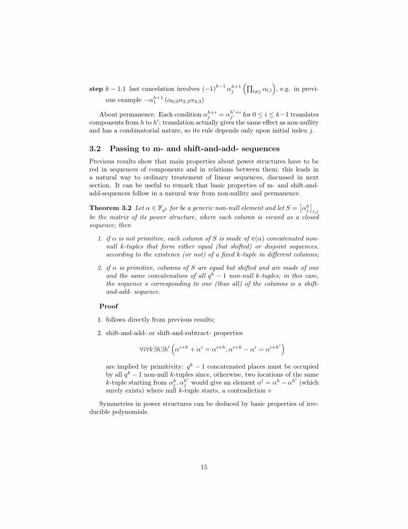
be the matrix of its power structure, where each column is viewed as a closedsequence; then

1. if α is not primitive, each column of S is made of π(α) concatenated non-null k-tuples that form either equal (but shifted) or disjoint sequences,according to the existence (or not) of a fixed k-tuple in different columns;

2. if α is primitive, columns of S are equal but shifted and are made of oneand the same concatenation of all qk − 1 non-null k-tuples; in this case,the sequence s corresponding to one (thus all) of the columns is a shift-and-add- sequence.

Proof

1. follows directly from previous results;

2. shift-and-add- or shift-and-subtract- properties

∀i∀k∃h∃h′(αi+k + αi = αi+h, αi+k − αi = αi+h′

)are implied by primitivity: qk − 1 concatenated places must be occupiedby all qk − 1 non-null k-tuples since, otherwise, two locations of the samek-tuple starting from αh

j , αh′

j would give an element αl = αh−αh′ (whichsurely exists) where null k-tuple starts, a contradiction

Symmetries in power structures can be deduced by basic properties of irre-ducible polynomials.

15

3.3 Some enumerations

Complete power structures show four obvious symmetries, combined by inver-sion of components and inversion of recyprocal polynomials

(x0; . . . ;xk−1)←→ (tk−1; . . . ; t0)

xk ≡ a0 + a1x+ . . .+ ak−1xk−1

1 ≡ a0tk + a1t

k−1 + . . .+ ak−1t

tk ≡ a−10 − a1a

−10 t− . . .− ak−1a

−10 tk−1

with substitutions

a′0 = a−10

a′l = −ak−la−10 for 1 ≤ l ≤ k − 1

One may ask whether enumeration of relative shifts amongst maximal se-quences equals counting of irreducible polynomials times number of primitiveelements in a field representation, that is

Nq (k)φ(qk − 1

)=φ(qk − 1

)k

∑d|q

µ (d) qk/d

Without deeper considerations, a trivial result can be stated for qk = p2,since all possible choices for 1 are p and possible choices for 0 are p − 1; thus,power structures for Fp2 simply come out from each relative shift between twoinstances of the same shift-and-add-sequence, giving element “10” in some place:

12[µ(1)p2 + µ(2)p

]φ(p2 − 1) =

p2 − p2

(p2 − 1)

Exact counting will be proved in section 4 to hold for a general Fpk over Fp

and only in section 5 it will be sketched for a general subfield relation.Note that, for a choosen relative shift amongst maximal sequences, a squaring

condition can always be tested, since tuples (1; 0; . . . ; 0), . . . , (0; 0; . . . 1) must be

16

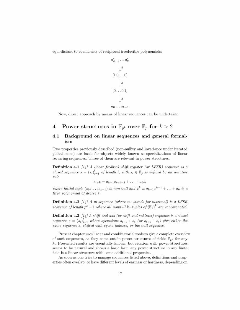
equi-distant to coefficients of reciprocal irreducible polynomials:

a′k−1 . . . a′0yd

[1 0 . . . 0]yd

[0 . . . 0 1]yd

a0 . . . ak−1

Now, direct approach by means of linear sequences can be undertaken.

4 Power structures in Fpk over Fp for k > 2

4.1 Background on linear sequences and general formal-ism

Two properties previously described (non-nullity and invariance under iteratedglobal sums) are basic for objects widely known as specializations of linearrecurring sequences. Three of them are relevant in power structures.

Definition 4.1 [14] A linear feedback shift register (or LFSR) sequence is aclosed sequence s = (si)

li=1 of length l, with si ∈ Fp is defined by an iterative

rulesi+k = ak−1si+k−1 + . . .+ a0si

where initial tuple (s0; . . . ; sk−1) is non-null and xk ≡ ak−1xk−1 + . . .+ a0 is a

fixed polynomial of degree k.

Definition 4.2 [14] A m-sequence (where m- stands for maximal) is a LFSRsequence of length pk − 1 where all nonnull k−tuples of (Fp)k are concatenated.

Definition 4.3 [14] A shift-and-add (or shift-and-subtract) sequence is a closedsequence s = (si)

li=1 where operations si+1 + si (or si+1 − si) give either the

same sequence s, shifted with cyclic indexes, or the null sequence.

Present chapter uses linear and combinatorial tools to give a complete overviewof such sequences, as they come out in power structures of fields Fpk for anyk. Presented results are essentially known, but relation with power structuresseems to be natural and shows a basic fact: any power structure in any finitefield is a linear structure with some additional properties.

As soon as one tries to manage sequences listed above, definitions and prop-erties often overlap, or have different levels of easiness or hardness, depending on

17

the point of view: e.g., shift-and-add definition is trivially an ultimate propertyof sequences of components of primitive elements and, for a given non-primitiveelement, Gauss’ algorithm makes a proper mixing of these properties, up to aprimitive element.

An example with low complexity can be examined: let F33 be representedby x3 ≡ 1 + x+ x2 irreducible over F3; power structure for x is:

x1 → (0; 1; 0) x8 → (1; 2; 0)x2 → (0; 0; 1) x9 → (0; 1; 2)x3 → (1; 1; 1) x10 → (2; 2; 0)x4 → (1; 2; 2) x11 → (0; 2; 2)x5 → (2; 0; 1) x12 → (2; 2; 1)x6 → (1; 0; 1) x13 → (1; 0; 0)

sequences(xi

0

)i,(xi

2

)i = σ are the same,(xi

1

)= τ is both their shift-and-add

and shift-and-subtract counterpart; Gauss’ algorithm applied to xi−xi−1 gives:

(0;1;0) → x2 − x1 ≡ (0; 2; 1) →(x2 − x1

)2 ≡ (1; 2; 2)

(0; 0; 1) → x3 − x2 ≡ (1; 1; 0)... (2; 0; 1)

(1; 1; 1)... (0; 1; 1)

... (1; 0; 1)

(1; 2; 2) (1; 1; 2)... (1; 2; 1)

(2; 0; 1) (2; 0; 0) (1; 2; 0)(1; 0; 1) (0; 2; 0) (0; 1; 2)(1; 2; 1) (0; 0; 2) (2; 2; 0)(1; 2; 0) (2; 2; 2) (0; 2; 2)(0; 1; 2) (2; 1; 1) (2; 2; 1)(2; 2; 0) (1; 0; 2) (1; 0; 0)(0; 2; 2) (2; 0; 2) (0;1;0)(2; 2; 1) (2; 1; 2) (0; 0; 1)(1; 0; 0) (2; 1; 0) (1; 1; 1)

with notations as in chapter 2, choose b2 = a3 and l = 0 so a primitiveelement is built up with its power table and the same sequence comes out in allcomponents:

Stability under global sums or differences is an inner property of the se-quence, not strictly related to a fixed primitive element; so, the most importantstep is to change point of view inside a power table and to look at sequencesalong components. Defining the order of a polynomial p(x) as lowest e suchthat f(x)|xe − 1, following known results are extracted from [14] and [20]:

Theorem 4.1 1. Any irreducible polynomial p(x) of degree k and order eover Fp outcomes a LFSR sequence of length e;

2. nonnull k−tuples over Fp are partitioned in classes, each with cardinalitye;

18

↓α ↓β ↓γ ↓δ ↓ε ↓ζ0 1 0 0 2 00 2 1 0 1 21 2 2 2 1 11 1 2 2 2 11 2 1 2 1 20 0 2 0 0 12 2 0 1 1 01 0 2 2 0 11 0 0 2 0 02 1 0 1 2 01 1 1 2 2 20 1 1 0 2 21 0 1 2 0 2↓δ ↓ε ↓ζ ↓α ↓β ↓γ

3. if q(x) is primitive, resulting sequence is a m-sequence;

4. each m-sequence is a shift-and-add sequence.

Remark 4.1 - Counting irreducible polynomials of degree k can be performedby two different formulas, namely∑

d|k

µ (d) pk/d =∑

e|(pk−1)e-(ph−1),h|k

φ (e)

where φ (e) /k counts irreducible polynomials of degree k and order e. Relationabove is a simple application of inclusion-exclusion principle for k = k1 · . . . · kn

and elementary property pk − 1 =∑

e|(pk−1) φ (d) and it is relevant since, for kfixed, orders e avoid values e|

(ph − 1

)for h|k and this happens if and only if a

given power structure entirely falls in subfield Fph , so a lower degree polynomialand a LFSR subsequence are involved. This situation is fully studied in chapter5.

Results from previous chapter show that these properties can be as welldeduced if initial requirements are restricted to non-nullity and permanence;any further completion using Gauss’ algorithm gives a proper shift-and-addsequence. But non-nullity and permanence for α generic have shown to be awfulproperties, so a purely combinatorial generalization from x to any α primitiveis available:

1. non-nullity and permanence for x primitive follow from linear recurrence;

2. sequences in components of power tables for xpl

(these elements are usuallycalled Galois conjugates) are the same as for x, ∀1 ≤ h ≤ k − 1;

19

3. wheneverxidk−1

i=1are linearly independent, base change

xik−1

i=1→

xidk−1

i=1gives a power table with the same sequence;

4. previous steps fulfill enumeration of primitive roots for Fph over Fp.

Matricial notation is as in chapter 3 and special case α = x allows easiertools.

• Matrix B(x), performing product a · x = a · B(x), is usual companionmatrix for polinomial p(x) (see [20]) with changed signs:

B(x) =

0 1 0 . . . 00 0 1 0 . . . 0...

.... . .

0 0 . . . 1a0 a1 . . . ak−1

where (bi,j)k−1

j=0 contains coefficients of xi as as vector and last row givesxk ≡ a0 + . . .+ ak−1x

k−1;

• global matrix M(x) =[xi

j

](π(x);k−1)

(i;j)=(1;0)of order π(x) × k, containing all

powers of x as rows, has B(x) as first block.

Properties of M(x) are:

1. (Reduction to previous row)

xij = xi−1

j−1 + xk−1j−1aj (1)(

xij

)k−1

j=0=(xi−1

j

)k−1

j=0·B(x) (2)

(3)

2. (Reduction up to first row) - Each element xij or α(h)

i,j can be written as

a row-column product where row shifts from(xi−1

j

)k−1

j=0to lower powers(

xi−lj

)k−1

j=0while column shifts from

(x1+l

j

)k−1

l=0to higher powers

(xi

j

)k−1

j=0,

as far as row(xk

j

)k−1

j=0and element xi−1

j in column are reached:

xij =

(xi−1

0 ; . . . ;xi−1k−1

)·(x1

j ; . . . ;xkj

)=

=(xi−2

0 ; . . . ;xi−2k−1

)·(x2

j ; . . . ;xk+1j

)=

=(xk

0 ; . . . ;xkk−1

)·(xi−k

j ; . . . ;xi−1j

)

20

last equality simply means a restatement of recurrence relation, shiftedalong rows and columns:

xij = a0x

i−kj + . . .+ ak−1x

i−1j

3. linear independence∣∣(xh+i

j

)∣∣ 6= 0 for each continuous block with h fixedand i, j = 0 . . . k − 1 follows since∣∣(xh+i

j

)∣∣k−1

i,j=0=∣∣(xi

j

)∣∣k−1

i,j=0·∣∣Bh(x)

∣∣ = 1 · |B(x)|h =(

(−1)ka0

)h

6= 0

Matrix B (α) performing product by any α and higher powers Bh (α) can beviewed as layers of a 3D-matrix where B (x) = B0 (α) is front layer B0(α)∀α;following usual notation αh

i,j for a general entry of Bh (α), reductions and prop-erties similar to M (x) may be useful:

1. (Reduction to previous row)[αh

i,j

]j

=[αh

i−1,j−1

]j

+ αhi−1,k−1 [aj ]j

2. (Reduction up to first row)

αhi,j =

(αh

i−1,0; . . . ;αhi−1,k−1

)·(x1

j ; . . . ;xkj

)=

=(αh

i−2,0; . . . ;αhi−2,k−1

)·(x2

j ; . . . ;xk+1j

)=...

=(αh

0,0; . . . ;αh0,k−1

)·(xi

j ; . . . ;xi+k−1j

)3. linear independence

∣∣(αh+ij

)∣∣ 6= 0 is a special quest, often superseded byenumerations to be explained.

According to this notation, power αh is in 0-th row of Bh (α) and powertable for α is upper face of the parallepiped.

4.2 Power structures for x

Information in power structure of element x can be easily deduced from non-nullity and permanence.

Lemma 4.1 Let B (x) ,M (x) be power structures for x ∈ Fph ; then:

1. (Non-nullity) - for any fixed component 0 ≤ j ≤ k− 1 and any 1 ≤ h ≤π(x), system of conditions

xh+lj = 0 for 0 ≤ l ≤ k − 1

implies xh+kj = 0, impossible for given assumptions;

21

2. (Permanence) - for any fixed components 0 ≤ j, j′ ≤ k− 1, if h, h′ existsuch that

xh+lj = xh′+l

j′ for 0 ≤ l ≤ k − 1

then xh+kj = xh′+k

j′ .

Proof - About non-nullity, if xh+lj = 0 for 0 ≤ l ≤ k − 1, then

xh+kj =

(xh+k−1

0 ; . . . ;xh+k−1k−1

)·(x1

j ; . . . ;xkj

)= . . .

=(xk

0 ; . . . ;xkk−1

)·(xh

j ; . . . ;xh+k−1j

)= 0

and whole sequence(xh

j

)pk−1

h=1would be null.

About permanence, if xh+lj = xh′+l

j′ for 0 ≤ l ≤ k − 1 then

xh+kj =

(xh+k−1

0 ; . . . ;xh+k−1k−1

)·(x1

j ; . . . ;xkj

)= . . .

=(xk

0 ; . . . ;xkk−1

)·(xh

j ; . . . ;xh+k−1j

)=

=(xk

0 ; . . . ;xkk−1

)·(xh′

j′ ; . . . ;xh′+k−1j′

)= . . .

=(xh′+k−1

0 ; . . . ;xh′+k−1k−1

)·(x1

j′ ; . . . ;xkj′)

= xh′+kj′ .

Relation between irreducible polynomials and full power structures can thusbe stated.

Theorem 4.2 Let Fph be represented by p(x) of order e, so that x has periodπ (x) = e; then

1. columns(xi

j

)π(x)

i=1in power table for x are LFSR sequences generated by

p(x) and either are equal but shifted or have no common concatenatedk-tuples;

2. if p is primitive (thus x is a primitive root), columns(xi

j

)pk−1

i=1are equal

but shifted and are built of the m-sequence generated by p.

Proof - Follows directly from previous lemmas.

Enumeration of primitive polynomials isφ(pk − 1

)k

and recyprocal polyno-mials can be put together, so a complete example with low complexity can be

F34 over F3, to haveφ(80)

4= 4 distinct m-sequences listed in tables 2 to 5, each

with its own couple of primitive polynomials.

4.3 Reduction of sequences for xpland decimations

Any α primitive is often considered together with what are called its Galoisconjugates αpl

, 2 ≤ l ≤ k − 1, which are also primitive. It can be shown that

22

→ε 1 0 0 0 1 0 0 2 1 0 1 1 1 2 0 0 →α

→α 2 2 0 1 0 2 2 1 1 0 1 0 1 2 1 2 →β

→β 2 1 2 0 1 2 2 2 2 0 0 0 2 0 0 1 →γ

→γ 2 0 2 2 2 1 0 0 1 1 0 2 0 1 1 2 →δ

→δ 2 0 2 0 2 1 2 1 1 2 1 0 2 1 1 1 →ε

Table 2: sequence s1, x4 ≡ 1 + 2x⇔ x4 ≡ 1 + x3

→ε 1 0 0 0 1 0 0 1 1 0 1 2 1 1 0 0 →α

→α 2 1 0 2 0 1 2 2 1 0 1 0 1 1 1 1 →β

→β 2 2 2 0 1 1 2 1 2 0 0 0 2 0 0 2 →γ

→γ 2 0 2 1 2 2 0 0 1 2 0 1 0 2 1 1 →δ

→δ 2 0 2 0 2 2 2 2 1 1 1 0 2 2 1 2 →ε

Table 3: sequence s2, x4 ≡ 1 + x⇔ x4 ≡ 1 + 2x3

→ε 1 0 0 0 1 2 2 1 1 1 0 0 2 2 0 1 →α

→α 0 0 1 0 1 0 2 2 1 0 2 1 2 1 1 0 →β

→β 1 1 1 1 2 1 0 1 2 0 0 0 2 1 1 2 →γ

→γ 2 2 0 0 1 1 0 2 0 0 2 0 2 0 1 1 →δ

→δ 2 0 1 2 1 2 2 0 2 2 2 2 1 2 0 2 →ε

Table 4: sequence s3, x4 ≡ 1 + x+ x2 + 2x3 ⇔ x4 ≡ 1 + x+ 2x2 + 2x3

→ε 1 0 0 0 1 1 2 2 1 2 0 0 2 1 0 2 →α

→α 0 0 1 0 1 0 2 1 1 0 2 2 2 2 1 0 →β

→β 1 2 1 2 2 2 0 2 2 0 0 0 2 2 1 1 →γ

→γ 2 1 0 0 1 2 0 1 0 0 2 0 2 0 1 2 →δ

→δ 2 0 1 1 1 1 2 0 2 1 2 1 1 1 0 1 →ε

Table 5: sequence s4, x4 ≡ 1 + 2x+ x2 + x3 ⇔ x4 ≡ 1 + 2x+ 2x2 + x3

23

they share the same m-sequence as α. Due to a basic property of characteristicp:

(a+ b)p = ap + bp in any Fpk

This leads to a general reduction of p-powers as vectors:

xhpl

=(xh

0 + xh1x+ . . .+ xh

k−1xk−1)pl

= xh0x

0 + xh1x

pl

+ . . .+ xhk−1x

(k−1)pl

where exponents cannot be further reduced since they refer to rows of matrixM(x). So, for x primitive, defining properties of a primitive sequence may beproved for sequences of xpl

:Non-nullity: previous condition, written on compontents, means

xhpl

j =(xh

0 ; . . . ;xhk−1

)·(x0

j ;xpl

j ; . . . ;x(k−1)pl

j

)thus

x

(h+i)pl

j = 0 for 0 ≤ i ≤ (k − 1) becomes a system in xipl

j ’s:(xh+i

m

)m·(xmpl

j

)m

= 0 i = 0, . . . , k − 1

whose determinant∣∣∣∣∣∣∣xh

0 . . . xhk−1

.... . .

...xh+k−1

0 . . . xh+k−1k−1

∣∣∣∣∣∣∣ =

∣∣∣∣∣∣∣∣(xh

j

)j

...(xh+k−1

j

)j

∣∣∣∣∣∣∣∣is 6= 0 since rows are a continuous block of M(x); then xipl

j = 0 ∀i is the

only solution, a contradiction since above formula for xhpl

j would imply(xhpl

j

)j

to be a null sequence.

Pulling down to xij : since

(xhpl

j

)pk−1

h=1satisfies non-nullity, any of its seg-

ments of length k has one and only one location in(xi

j

)pk−1

i=1; fixed initial segment(

x0j ;xpl

j ; . . . ;x(k−1)pl

j

), ∃! hl such that(

xipl

j

)k−1

i=0=(xhl+i

j

)k−1

i=0

Thus, for each subsequent xhpl

j one can apply usual reduction rules for M(x):

xhpl

j =(xh

0 ; . . . ;xhk−1

)·(x0

j ; . . . ;x(k−1)pl

j

)=

=(xh

0 ; . . . ;xhk−1

)·(xhl

j ; . . . ;xhl+k−1j

)= xh+hl

j

Non-nullity holds in a more general situation, where the question about anypower structure can be put and answered.

24

Corollary 4.1 In power table M(x) for x primitive, let α be a generic elementsuch that αd(h+i) for i = 0, . . . , k − 1 are linearly independent; then, for anyl = 1, . . . , k − 1 and j fixed, system

0≤i≤(k−1)αd(h+i)pl

j = 0

is incompatible with initial assumptions.

Proof - Explicitation of(α

d(h+i)0 + α

d(h+i1 x+ . . .+ α

d(h+i)k−1 xk−1

)pl

gives sys-tem

0≤i≤(k−1)

(α

d(h+i)0 ; . . . ;αd(h+i)

k−1

)·(x0

j ;xpl

j . . . ;x(k−1)pl

j

)= 0

whose determinant ∣∣∣∣∣∣∣αdh

...αd(h+k−1)

∣∣∣∣∣∣∣is 6= 0, implying impossibility. Now, one can partition exponents 1 ≤ d ≤ pk − 1 in four classes:

1. d = pl, thus counted by φ(pk − 1);

2. remaining d 6= pl counted by φ(pk − 1);

3. d = l∑k|h

i=0 pk−ih for 1 ≤ l ≤ ph − 1 and h|k;

4. d out of previous cases.

Power structures show to be strongly sensible to previous classification ofd’s and each power structure can be defined in a suitable way, starting fromstructures for x primitive. As a basic fact of finite fields, rows of M(x) can bepermuted according to exponents d counted by φ(pk−1); a purely combinatorialoperation on rows in M(x) is frequently appled to sequences of components.

Definition 4.4 Let s be a given m-sequence of length pk−1 and d = 1 . . . pk−2fixed; then, let MCD(d; pk−1) = e so that d = ef , pk−1 = eg for f, g relativelyprimes; then, a decimation φd is the map defined componentwise as

φd(s) =

(si+hd)g−1h=0 for 0 ≤ i ≤ (e− 1)

If a decimation φd is applied on a whole k−tuple, cyclic groups properties

seem to have a role superimposed to algebraic structure, but applications to am-sequence are interesting: they simply pick out of s values sh whose indiceslie at distance d and, for d and pk − 1 relatively primes, φd gives a new powerstructure. Main properties of φd are collected in a result quite obvious, thatenlights the ratio for such a definition:

25

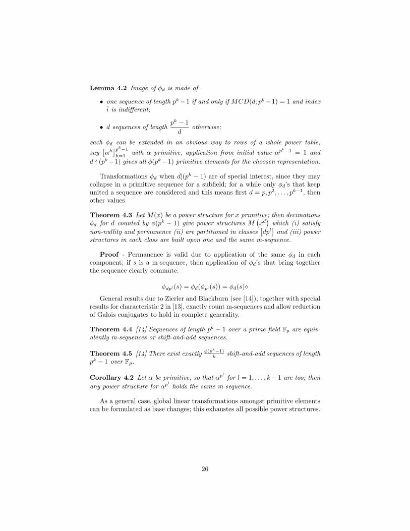
Lemma 4.2 Image of φd is made of

• one sequence of length pk−1 if and only if MCD(d; pk−1) = 1 and indexi is indifferent;

• d sequences of lengthpk − 1d

otherwise;

each φd can be extended in an obvious way to rows of a whole power table,

say[αh]pk−1

h=1with α primitive, application from initial value αpk−1 = 1 and

d - (pk−1) gives all φ(pk−1) primitive elements for the choosen representation.

Transformations φd when d|(pk − 1) are of special interest, since they maycollapse in a primitive sequence for a subfield; for a while only φd’s that keepunited a sequence are considered and this means first d = p, p2, . . . , pk−1, thenother values.

Theorem 4.3 Let M(x) be a power structure for x primitive; then decimationsφd for d counted by φ(pk − 1) give power structures M

(xd)

which (i) satisfynon-nullity and permanence (ii) are partitioned in classes

[dpl]

and (iii) powerstructures in each class are built upon one and the same m-sequence.

Proof - Permanence is valid due to application of the same φd in eachcomponent; if s is a m-sequence, then application of φd’s that bring togetherthe sequence clearly commute:

φdpl(s) = φd(φpl(s)) = φd(s)

General results due to Zierler and Blackburn (see [14]), together with specialresults for characteristic 2 in [13], exactly count m-sequences and allow reductionof Galois conjugates to hold in complete generality.

Theorem 4.4 [14] Sequences of length pk − 1 over a prime field Fp are equiv-alently m-sequences or shift-and-add sequences.

Theorem 4.5 [14] There exist exactly φ(pk−1)k shift-and-add sequences of length

pk − 1 over Fp.

Corollary 4.2 Let α be primitive, so that αpl

for l = 1, . . . , k− 1 are too; thenany power structure for αpl

holds the same m-sequence.

As a general case, global linear transformations amongst primitive elementscan be formulated as base changes; this exhaustes all possible power structures.

26

4.4 Base change over a whole power structure

Power structure in a finite field is always defined by means of a linear trans-formation, so ultimate representation is by means of base changes. Followingresult shows that primitive elements and irreducible polynomials are differentviews of one and the same structure built up by a fixed m-sequence.

Lemma 4.3 Let x be primitive and 1 ≤ d ≤ pk − 1 be fixed; then:

1. any system of vectorsxidk−1

i=0is a base if and only if xid’s don’t belong

to a subfield Fph ;

2. xid’s belong to a subfield if and only if d = l∑k|h

i=0 pk−ih for some l and

h|k;

3. number of distinct linearly idndependent systemsxid

is exactly countedby

kNp(k) =∑h|k

µ(h)pk/h

Proof

1. Let(xid)k−1

i=0be a base; then linear indipendence implies

∑k−1i=0 cix

id = 0if and only if ci = 0 ∀i, but for d = l

(ph − 1

)one has cyclic vectors, since

xd is a root of a polynomial of degree h|k, ∃co, . . . ch−1 not all = 0 suchthat xhd =

∑h−1i=0 cix

id and ch = . . . ck−1 = 0 can be added, contradictingprevious indipendence. Argument is clearly invertible, due to the samedefinition of subfield.

2. values d = l pk−1

ph−1lie cyclically in exponents satisfying basic rule h|k needed

for subfield relation.

3. Let k = kα11 . . . kαl

l be prime decomposition of exponent k non-prime; eachh|k gives values

d = l(pk−h + pk−2h + . . .+ p+ 1

), 1 ≤ l ≤ ph − 1

that have to be treated according to inclusion exclusion rules, so theircoefficient in global counting is µ

(kh

)and∑

h|k

µ

(k

h

)(ph − 1

)=∑h|k

µ

(k

h

)ph −

∑h|k

µ

(k

h

)=∑h|k

µ(h)pk/h

Recurrence relation and ordinary base change give biggest set of transfor-mations that leave a m-sequence unchanged. Any power structure S for xprimitive can be simply viewed as a (pk − 1) × k matrix where a base change(xi)k−1

i=07→(xid)k−1

i=0is applied; matrix A =

[(xo,j) ; (xd,j) ; . . . ;

(x(k−1)d,j

)]has

columns related to inverse base change, so one can compute A−1, transpose itand look at S ×

(A−1

)t as a new power structure, obtained by means of purelylinear tools.

27

Theorem 4.6 Let x be primitive, with S associated global power structure; letT (xi) = xid, 0 ≤ i ≤ k − 1 be any base change amongst linearly independent,regularly located powers of x and T−1(xi) = xti be inverse base change; then

1. matrix products S′ = S × T (xi) and S′′ = S × T−1(xi) give other powerstructures;

2. resulting power structures are different from those derived by cyclicityproperties, except for base change T (xi) = xip, which gives the same resultas for transformation φd;

3. S′ and S′′ are built upon the same primitive sequence as S.

Proof

1. Completeness of power structures S′, S′′ is given by two facts: T, T−1 arebijections over F×

pk and they correspond to a reduction

xkd ≡ a0 + a1xd + . . .+ ak−1x

(k−1)d

always valid since p(x) is irreducible.

2. Definition of T forxi7→xip

is the same as φp over x0, . . . , xk−1:

T(xi)j

=(xi

0; . . . ;xik−1

)·(x0

j ; . . . ;x(k−1)pj

)= φp

(xi)

and φp is linear since (λa+ µb)p = λap + µbp.

3. Let T (xi) = xid, 0 ≤ i ≤ k−1 be a fixed base change as above; by linearity,one has

T(xh)

= xh0 + xh

1xd + . . .+ xh

k−1x(k−1)d

or, in components,

T(xh)j

=(xh

0 ; . . . xhk−1

)·(x0

j ;xdj ; . . . ;x(k−1)d

j

).

First, non-nullity holds: condition T(xh+h

)= 0 for 0 ≤ h ≤ (k−1), that

is (xh+h

0 ; . . . xh+hk−1

)·(x0

j ;xdj ; . . . ;x(k−1)d

j

)= 0, 0 ≤ h ≤ (k − 1)

this is a system in x0j , x

dj , . . . , x

(k−1)dj whose matrix, a sequence of h consec-

utive powers of x, cannot have null determinant; so xidj = 0, 0 ≤ h ≤ (k−1)

is the only solution, a contradiction since it is a column of matrix withxid’s, that is a base.

Then ∃!h1 such that T (x0)j = xh1j , T (x1)j = xh1+1

j , . . . , T (xk−1)j =xh1+k−1

j and subsequent power k is

28

T (xk)j =(xk

0 ; . . . xkk−1

)·(x0

j ;xdj ; . . . ;x(k−1)d

j

)=

=(xk

0 ; . . . xkk−1

)·(T (x0)j ;T (x1)j ; . . . ;T (xk−1)j

)=

=(xk

0 ; . . . xkk−1

)·(xh1)j ;xh1+1

j ; . . . ;xh1+k−1j

)= xh1+k

j

and T (xh)j = xh1+hj can be extended to any higher h, so for the whole

sequence one has S = S′. Inverse linear transformation can also beapplied, so that T−1(1) = 1, T−1(x) = α1 = xt1 , T−1(x2) = α2 =xt2 , . . . , T−1(xk−1) = αk−1 = xtk−1 where exponents ti have no knownrelation with i. General definition is, by linearity, T−1(xh) = xh

0 +xh1x

t1 +. . .+ xh

k−1xtk−1 and non-nullity is

T−1(xh+h)j = xh0x

0j + xh

1xt1j + . . .+ xh

k−1xtk−1j =

=(xh

0 ; . . . xhk−1

)·(x0

j ;xt1j ; . . . ;xtk−1

j

)= 0, 0 ≤ h ≤ (k − 1)

and x0j = xt1

j = . . . = xtk−1j = 0 is a contradiction, since it is a column

of a base change. Then ∃!h1 such that T−1(xh)j = xh1+hj and subsequent

power k is

T−1(xk)j =(xk

0 ; . . . xkk−1

)·(x0

j ;xt1j ; . . . ;xtk−1

j

)=

=(xk

0 ; . . . xkk−1

)·(T−1(x0)j ;T−1(x1)j ; . . . ;T−1(xk−1)j

)=

=(xk

0 ; . . . xkk−1

)·(xh1)j ;xh1+1

j ; . . . ;xh1+k−1j

)= xh1+k

j

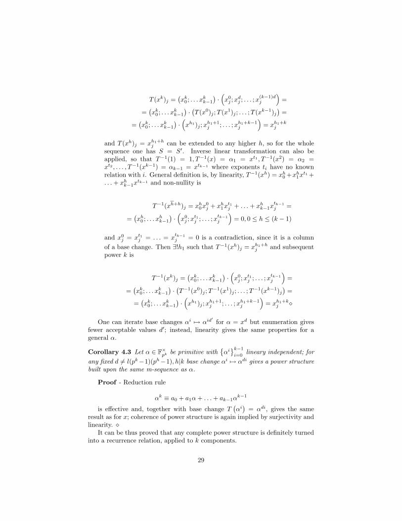
One can iterate base changes αi 7→ αid′ for α = xd but enumeration givesfewer acceptable values d′; instead, linearity gives the same properties for ageneral α.

Corollary 4.3 Let α ∈ F×pk be primitive with

αik−1

i=0lineary independent; for

any fixed d 6= l(pk−1)(ph−1), h|k base change αi 7→ αdi gives a power structurebuilt upon the same m-sequence as α.

Proof - Reduction rule

αk ≡ a0 + a1α+ . . .+ ak−1αk−1

is effective and, together with base change T(αi)

= αdi, gives the sameresult as for x; coherence of power structure is again implied by surjectivity andlinearity.

It can be thus proved that any complete power structure is definitely turnedinto a recurrence relation, applied to k components.

29

Corollary 4.4 For a fixed m-sequence, relative shifts amongst k instances giv-ing an effective power structure are determined by a location of elements αi = xdi

(from an initial configuration where x is primitive) and prosecuted component-wise by recurrence relation.

Proof - Once k rows αi = xdi are choosen, for each component an initialstate (si,j)j is fixed and recurrence relation sh = ak−1sh−1 + . . . + a0sh−k canbe started; linearity assumes, in each component, the same outcome as for abase change.

As a final step, a complete enumeration can be collected.

4.5 Concluding enumeration of power structures

Previous results can be collected in an enumeration to fullfill total number

φ(pk − 1

)k

∑d|k

µ (d) pk/d

of power structures for Fpk over Fp; enumeration can be made shortly upondecimations and, at least, partitioned in different m-sequences.

Theorem 4.7 Each ofφ(pk − 1)

kprimitive sequences of length pk−1 can build

Np(k) · k =∑d|kµ(d)pk/d correct power structures for Fpk over Fp; thus, global

counting φ(pk − 1)Np(k) always holds.

Proof - Enumeration∑d|kµ(d)pk/d can be applied to transformations φd for any

1 ≤ d ≤ (pk − 1), since any fixed φd falls into one and only one of followingcases:

1. if d 6= ph − 1 for all h|k, image of φd has cardinality MCD(d; pk − 1) andfragments form a partition of non-null k-tuples;

2. if d = ph−1 for some h|k, image of φd collapses in fragments made of eitherone (and the same) primitive sequence for a representation of subfield Fph ,or the null sequence (0i)i.

Transformations of type (1) correctly count all acceptable φd’s, but theyare used only to localize squaring conditions and they are not really applied;instead, transformations of type (2) have to be discarded, since they cannotbuild a structure of order (pk − 1).

Now, factorization of k = pα11 . . . pαn

n gives values of d that have to be dis-carded and product of pαi

i ’s exactly matches requests for µ-function:factorization (pk − 1) = (ppi − 1) · (pp

αi−1i + . . .+ 1) gives (ppi − 1) transfor-

mations φl(pp

αi−1i +...+1)

that have to be discarded; further exponents of pi are

30

indifferent, since they are included in previous counting; indifference of αi’s isthe same condition as µ(n) = 0 when n contains almost a square. So, only valuesd|k that are products of distinct pi’s count, with usual sums or subtractions inorder to balance multiple countings; a direct application of Inclusion-ExclusionPrinciple gives total counting of acceptable φd’s:

(pk−1)−∑

|T |=n−1

(p

∏i∈T pi − 1

)+

∑|T |=n−2

(p

∏i∈T pi − 1

)−. . .+(−1)n

n∑i=1

(ppi − 1)

where (−1)’s can be collected and cancelled, since their total number is

n∑l=0

(n

l

)(−1)l = 0

for a basic property of bynomials. Thus, previous counting gives same terms as∑d|kµ(d)pk/d.

Corollary 4.5 For any fixed m-sequence of length pk − 1, following completepower structures can be built:

• Build an m-sequence s1 of length pk − 1 over Fp; checksum of elements(δij

)k−1

j=0at distance 1 gives basic structure for x primitive and identifies

primitive recyprocal polynomials p(x), p(x).

• Transformations φpl for 1 ≤ l ≤ (k− 1) hold the same sequence s1; check-

sum of elements(δij

)k−1

j=0at distances pl give power structures for xpl

.

• Transformations φd for d counted by φ(pk−1) give power structures parti-tioned in m-sequences s2, . . . , sφ(pk−1)/k according to classes

[dpl]; check-

sum of elements(δij

)k−1

j=0at distance d is locked since primitive polynomials

p(x), p(x) don’t change under these operations.

• Transformations in previous step can be cyclically applied (e.g. to imagesof φd(s) or by means of base changes

xdi→xi); a set of power

structures of cardinality(φ(pk − 1)

)2/k is defined; the same cardinality

is given by checksums of elements(δij

)k−1

j=0at distances d along all m-

sequences; irreducible polynomials involved are all primitive.

• For d not counted by φ(pk − 1) and d 6= l pk−1

ph−1with h|k, base changes

xdi→xi

hold the same initial m-sequence si and fulfill remaining

φ(pk − 1)k

∑d|k

µ(d)pk/d − φ(pk − 1)

31

power structures; the same cardinality is given by checksums of elements(δij

)k−1

j=0at distances d along all m-sequences; all irreducible polynomials

involved have order e < (pk − 1).

5 Subfield relation Fph → Fpk for h|kDistinct representations of a subfield Fph → Fpk are all isomorphic and, aftera theorem of Blackburn (see [14]), quest for shift-and-add- or m- propertiesimplies that m-sequences over ground field Fp have always to be considered.But any Fpk can also be built upon a fixed Fph , required to be stable; this maygive chains of subfields, for a fixed decomposition k = h1 . . . kl. Stability of asubfield is proved to give specific relative shifts amongst blocks of m-sequences.

5.1 General construction of power sub-structures

Following result collects basic results.

Lemma 5.1 Let α ∈ Fpk be a primitive element, M (α) be the matrix of itspower structure, with m-sequence s and k = hl, e =

(pk − 1

)/(ph − 1

); then

1. matrix M(αei)

for 1 ≤ i ≤ ph−1 is a power structure for (a representationof) a subfield Fph ;

2. columns of M(αei)

are made of either one and the same m-sequence t oflength ph − 1 or the null sequence;

3. equally shifted rows M(αei+r

)are made of either the same sequence t or

the null sequence, thus s is uniquely determined as an extension of t.

Proof

1. Elements αei satisfy(αei)ph−1 = 1, that is a basic property defining Fph ,

both for additive and multiplicative structure.

2. Property ∀i1∀i2∃i3(αei1 + αei2 = αei3

)implies that components of add-

shift, placed e.g. in position αe + 1 = αei, thus they are made of eitherone and the same recurrence relation

ti = b0ti−h + . . .+ bh−1ti−1

or everywhere null values. It is worth noting that this recurrence is definedin h values but holds in k components (apart from everywhere null ones).

3. Segmentation of s at distances e means that a decimation φe has beenapplied, so proof of this part can be given for α = x, that is for a primitive

polynomial. Fix 1 ≤ r ≤ e− 1 and extract rows(xei+r

)ph−1

i=1from M(x);

recurrence relation holds for xeij , that is

xeij = bh−1x

e(i−1)j + . . .+ b0x

e(i−h)j ;

32

let(xr

j ; . . . ;x(h−1)e+rj

)be an initial segment, assumed to be 6= 0; then ∃!

position ir,j such that x(ir,j+l)e)j = xle+r

j for 0 ≤ l ≤ h − 1. Subsequentvalue xhe+r

j can be computed for xhe+r = xhl ·Br(x), where

xhe+rj =

(h−1∑i=0

bixie0 ; . . . ;

h−1∑i=0

bixiek−1

)·(xr

j ; . . . ;xr+k−1j

)=

=h−1∑i=0

bi(xie

0 ; . . . ;xiek−1

)·(xr

j ; . . . ;xr+k−1j

)=

= b0xrj + . . .+ bh−1x

(h−1)e+rj =

= b0xir,jej + . . .+ bh−1x

(ir,j+h−1)ej = x

(ir,j+h)ej

and recurrence relation can be extended along the whole component. Ifinitial segment is null, last equivalence means x(ir,j+h)e

j = 0.

Decimations φd for d = l(pk − 1

) (ph − 1

)were left aside in previous chap-

ters, so full information for any d is now explained.

5.2 Power structures for Fpk with a stabilized subfield Fph

Special structures for Fpk can be built upon an exact representation of Fph ;this happens together with a precise phoenomenology: power structure of Fph

is surrounded by everywhere null components; algebraic equivalent is a systemof (almost) two reductions

xh ≡ a0 + . . .+ ah−1xh−1, ai ∈ Fp

yl ≡ b0 + . . .+ bl−1yl−1, bi ∈ Fph

...

that can be studied in detail.

5.2.1 Representations of Fpk with a Fph stable

When a power structure for Fpk is built upon a power structure for a standardFph , elements of the latter appear in l copies and are everywhere surroundedby null components. One may say that these structures stabilize subfield Fph .Since shift-and-add properties and maximal linear recurring properties on h-tuples hold also in each component, stabilization of a subfield implies a strongerregularity between m-sequences.

When Fpk is built upon Fp, relative shifts between components have beenpreviously related to alighment of block

(δij

)at equal distances; this makes

relative shifts everywhere different and shift-and-add property does not holdbetween h-tuples. But if a subfield Fph has to be stabilized, one and the same

33

shift-and-add property must hold between h-tuples; this implies a specific sim-metry in relative shifts inside h-tuples: they are obtained by a power structurefor Fpk blowing at distance

(pk − 1

)/(ph − 1

).

Relative shifts σ1, . . . σh−1 referred to e.g. first column are related to shiftsτ1, . . . τh−1 by rule

σi = τi(pk − 1

)/(ph − 1

)and each m-sequence for Fph seems to blow in

φ(pk − 1

)h

kφ (ph − 1)m-sequences for

Fpk .A phœnomenology of stabilized subfields takes into account partitioned pe-

riods [mpn] for 1 ≤ m ≤ pk − 1 and n|k, where n is least integer such thatmpn ≡ m mod pk − 1.

Number an of classes with period n is given by empirical rule[a1 = pk − p

ad = 1d

(pd − p−

∑n|d nan

)∀ d|k

this enumeration is however superseded by a more complete one, where a powerstructure for Fpk can be blowed from a power structure for some Fph .

5.2.2 Enumeration of sub-structures for Fpk with a Fph stable

If a complete enumeration of power structures for Fpk with a stable Fph isrequired, exact number

φ(pk − 1

)Np(h)Nph(l)

can be reached with following steps:

1. power structures for Fph are

φ(ph − 1

)Np(h) =

φ(ph − 1

)h

(hNp(h))

2. each m-sequence t of length ph − 1 blows inφ(pk − 1

)lφ (ph − 1)

m-sequences s of

length pk − 1 and the same happens for a whole power structure;

3. relative shifts amongst l blocks of h instances of s follow the same rule asdescribed in section 4, with lNph(l) acceptable relative shifts; this givestotal number

φ(pk − 1

)lφ (ph − 1)

φ(ph − 1

)Np(h)lNph(l)

same as above.

34

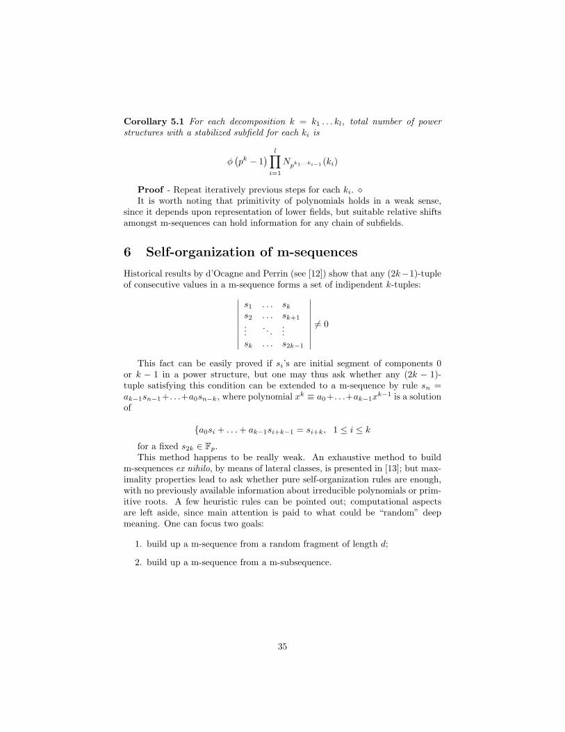
Corollary 5.1 For each decomposition k = k1 . . . kl, total number of powerstructures with a stabilized subfield for each ki is

φ(pk − 1

) l∏i=1

Npk1...ki−1 (ki)

Proof - Repeat iteratively previous steps for each ki. It is worth noting that primitivity of polynomials holds in a weak sense,

since it depends upon representation of lower fields, but suitable relative shiftsamongst m-sequences can hold information for any chain of subfields.

6 Self-organization of m-sequences

Historical results by d’Ocagne and Perrin (see [12]) show that any (2k−1)-tupleof consecutive values in a m-sequence forms a set of indipendent k-tuples:∣∣∣∣∣∣∣∣∣

s1 . . . sk

s2 . . . sk+1

.... . .

...sk . . . s2k−1

∣∣∣∣∣∣∣∣∣ 6= 0

This fact can be easily proved if si’s are initial segment of components 0or k − 1 in a power structure, but one may thus ask whether any (2k − 1)-tuple satisfying this condition can be extended to a m-sequence by rule sn =ak−1sn−1+. . .+a0sn−k, where polynomial xk ≡ a0+. . .+ak−1x

k−1 is a solutionof

a0si + . . .+ ak−1si+k−1 = si+k, 1 ≤ i ≤ k

for a fixed s2k ∈ Fp.This method happens to be really weak. An exhaustive method to build

m-sequences ex nihilo, by means of lateral classes, is presented in [13]; but max-imality properties lead to ask whether pure self-organization rules are enough,with no previously available information about irreducible polynomials or prim-itive roots. A few heuristic rules can be pointed out; computational aspectsare left aside, since main attention is paid to what could be “random” deepmeaning. One can focus two goals:

1. build up a m-sequence from a random fragment of length d;

2. build up a m-sequence from a m-subsequence.

35

6.1 Starting from random fragments

6.1.1 Gauss’ algorithm applied to random d-tuples

Let a random non-null d-tuple (si)di=0, si ∈ Fp be given; one may ask whether it

is the sequence of any component in any power structure and whether an appli-cation of Gauss’ algorithm may give a full m-sequence. Following preliminaryrequests are necessary:

• p - d;

• converge occurs at lowest e such that d| (pe − 1)

• d-tuples too much regular (e.g. constant) are forbidden;

• cyclicity may be closed with second d-tuple, since any global sum is definedmodulo (a1; . . . ; ad) ≈ (a1 + c; . . . ; ad + c);

• as soon as an iteration breaks requirements of cardinality for some value0 . . . p− 1, computation cannot give an acceptable result.

Indeed, Gauss’ algorithm always works when full information is available,but in a random situation it simply computes power-like values

l∑n=0

(−1)n

(l

n

)ai+nh

at step l and for a fixed h, as far as a cyclicity is closed. The only interestingremark is as follows.

Proposition 6.1 Let (si)di=1 be a random d-tuple in Fp and let k be the least

exponent (if any) such that d|(pk− 1); if a representation for Fpk over Fp existssuch that (si)

di=1 is associated to a component in power table of an element with

period d, then Gauss’ algorithm gives a linear sequence of higher order or maybea m-sequence; this surely happens when initial tuple itself is a LFSR sequence.

Some examples with d prime can be given.

• Choose d = 5 and pick at random (1; 2; 2; 0; 1) over (F3), put it in columnand apply ai−ai−1 in subsequent columns; after 16 iterations the originalcomes back, so 5 · 16 = 80 = 34 − 1 elements have been generated, thatare a m-sequences for F34 . This example works in an optimal way, due tofactorization.

• In F33 one has 33 − 1 = 2 · 13, factor 2 isn’t enough and factor 13 is toomuch, so random 13-tuples give an unpredictable result, if randomnessdoes not give a 13-tuple linearly recurring.

• If (si)di=1 is a random tuple, d|(pk − 1) and exactly

(pk − 1

)iterations are

needed to give back (si) it’s a bad new, since (si ± si+l)pk−1 = si ± si+l

is a basic property of arithmetic modp and every iterated sum ends likethat. This may happen e.g. in F35 , with 35 − 1 = 2 · 112, if a 11-tuple ischoosen.

36

6.1.2 Effective algorithm with backtracking

Shift-and-add condition on k-tuples makes any m-sequence constructible with astep-by-step algorithm, that roughly searches for the first stability point underany cyclic sum; such a point may be for a non maximal linear sequence.

Definition 6.1 A (k+l)-tuple (s1; . . . ; sk+l) ∈ (Fp)k+l is acceptable if it verifiesno conditions contradicting global stability, that means:

• k-tuples (s1; . . . ; sk) , (s2; . . . ; sk+1) , . . . , (s1+l; . . . ; sk+l) are all non-nulland distinct;

• any fixed arbitrary cyclic sum (si ± si+j1 ± . . .± si+jm) between values

(not necessarily consecutive) gives k-tuples either everywhere null, or non-null and distinct.

An algorithm may simply backtrack acceptable tuples:

1. fix a non-null k-tuple (s1; . . . ; sk);

2. given an acceptable segment of length (k+ l− 1), entail a new value sk+l

and verify segment (si)k+li=1 be also acceptable;

3. as soon as a configuration is reached, where a segment (si)k+li=1 or any of its

cyclic sums share a common tuple, segment (si)k+li=1 has one and only one

completion to a candidate linear sequence, maximal or not; each furtherentailed value must give an acceptable segment;

4. as soon as a non acceptable segment is reached, change last value entailedor backtrack to change more than one;

At step (s1; . . . ; sk+l), possible global sums are:

(±si ± δ1si+1 ± . . .± δlsi+l)ki=1

where δj = 0, 1 is a Kroneker-like symbol; so, there are 2l+1 possible signsand

(2l − 1

)acceptable δj (since δj = 0 ∀j returns initial segment and is

discarded), so there are 2l+1(2l − 1

)possible iterated sums of length at least k:

indeed too much, but this algorithm only needs to reach a stable configuration asnear as possible. Factors of pk−1 have some relevance, so Mersenne primesMk =2k − 1 for k prime are worst examples and no subsequence can be reached; thisis perhaps the main reason why such structures are best used in criptography.

6.2 Starting from m-subsequences

Known results about decimation [14] take into account subfield relation Fph →Fpk for k = hl, with a given primitive element α ∈ Fpk and any ω ∈ Fpk ,along trace considerations; a m-sequence s of length pk − 1 is thus written as a(pk−h + . . .+ 1

)×(ph − 1

)matrix whose columns are either a m-sequence t of

37

length ph − 1 or a null sequence (pk−2h + . . . + 1 total occurrences). But onemay try to tuild s by a checksum involving t, using no upward knoledge. Shift-and-add/-subtract properties are yet the cornerstone and a special empiricalstructure comes out.

Definition 6.2 For k, h, l as above, a l-skeleton is a configuration of pk−2h +. . .+ ph + 1 positions in a closed sequence of length pk−h + . . .+ 1 such that:

1. there is one and only one largest block of l − 1 consecutive positions;

2. number of positions at distance d is the same ∀1 ≤ d ≤(pk−h + . . .+ ph

),

where distances need not to be counted in the same block.

A l-skeleton can be computed by an independent task and, as a relevant fact,m-subsequence t seems to occupy positions around a l-skeleton; moreover, let ψd

be a trasformation that exchanges columns of s for MCD(d; pk−h + . . .+1) = 1,that is nothing but a decimation on columns; obviously, property (2) of a l-skeleton is invariant under ψd and, for p, k low, property (1) is invariant too.As the most relevant fact, the shape of a l-skeleton is invariant under some ψd’sand empirical counting gives unproved formula

φ(pk − 1

)k

≈φ(ph − 1

)h

φ(pk−h + . . .+ 1

)φ (l)

where(pk−h + . . .+ 1

)/φ (l) is candidate total number of l-skeletons.

Given a l-skeleton and a m-sequence t as above, following heuristic tool iseffective for add/subtract checksum:

• fix a block of order(ph − 1

)× l

0 . . . 0 s1...

......

0. . . 0 sph−1

with only one non-null column;

• choose a checksum block of order(ph − 1

)× (l + 1)

B(i, j) =

si . . . si sj

si+1 . . . si+1 sj+1

......

...

si−1. . . si−1 sj−1

where first row is aligned with (0; . . . ; 0; s1) in previous block;

• each admissible location for B(i, j), where 1 ≤ i 6= j ≤ (l − 1), gives oneand only one completion in full matrix, as far as either s is completed ora wrong values occurs.

38

Exact control occurs at nearest boundary around empty colums where check-sum block is placed inside l-skeleton; dimension of this computation has beenno further investigated and it can be surely optimized.

6.3 Other combinatorial regularities

Remark 6.1 Fix a m-sequence for Fq2 and a matricial representation

→ 1 · · · 0 →→ α 0 →

.... . .

...→ α−1 · · · 0 →

with α primitive for Fq, columns from 1 (second index) to p − 1 are made oftransversal shifts of the first column (considered as cyclic) satysfing the condi-tions:

• tk + tp−k = q

• τ q−12

= q+12 , τ q−1

2 −k − τ q−12 +k = ±k where the sign is uniform for all k.

Such a regularity property allows to break down the number of combinationsfor transversal shifts and, since a regular location of 1 values implies a regularityfor all the others, an equivalent formulation for this property is: given two

consecutive zeroes 0i

p+1− 0i+1, for each value a one has:

0id←→ a

p+1−d←→ 0i+1 ⇔ 0(i− p+12 +d)

p+1−d←→ ad←→ 0(i− p−1

2 +d)

7 A path towards the Riemann Hypothesis

Since shift-and-add- properties are intrinsic in power structures modulo deci-mations, some concluding remarks open a glimpse on a physical scenario; basicelements for such a transition are:

• additive structure in Zn is a low-level interaction (“thermodynamical”)and allows to built an upper structure if and only if n is a prime;

• non-nullity and permanence are global self-organizational properties andallow iterative construction of m-sequences of order pk for any k;

• structural relation of m-sequences is invariance under global cyclic sums,that tend to be dissipative, but cannot change any m-sequence, due toshift-and-add- properties.

Wherever considerations about self-organization and stability can be carriedout, a way is open towards an operative definition where primes p, prime powerspk and composite integers n =

∏i p

αii are distinguished by means of a physical

39

dictionary, and processes of interaction (thus dynamics) between primes can beconsidered.

Such an opportunity is already written in elementary number theory itself:where is a prime number located ? and what does “where” means ? It meanssomething about additive location, but it is driven by multiplicative structure,so this property seems a bit frustrating: a prime is located in a position at thesame time fixed but undetermined (up to present knoledge) and this propertyinvolves a clear relation amongst primes: a prime falls wherever no lower prime(or any of its multiples) falls; one can try to write down such a rule as aninteraction (a dynamics) between primes that compute altogether theire relative(as an outcome of interaction) or absolute (because they are fixed) positions andRiemann’s ζ-function may have its place in such a frame.

7.1 Hilbert-Polya conjecture and its environement

In never-too-much-famous 8-pages Riemann’s paper [25] defined complex func-tion ζ(s) and posed known hypothesis (RH from now on) about location ofprime numbers; a great amount of theoretical work succeded, in order to attackthat conjecture on many battlefields. A deep suggestion was born from informalcommunications between Hilbert and Polya (see Odlyzko home page [23]) andthe outcome has been an idea fully immersed in Physics: RH would be true ifnon-trivial zeros are related to eigenvalues of some hermitian matrix.

Further research enlighted a strong similarity between statistics of zeroes andGUE eigenvalues (see [26]) and went on enough to give many expected properties(see [3]), together with a deep confirmation of GUE statistics for ζ-functionsover finite fields (see [17]). As a very relevant fact, physical analogies havebeen correctly posed in many aspects of Number Theory and, since scientificresearch often makes large amounts of analogies to become reality, some areashave grown, that can just be listed: Unified Field Theory, linked toRH via Non-commutative Geometry; black hole analogies, used to describe arithmeticity ingravitation theory; string theory and tools from p-adic and adelic Analysis.

The most prominent adherence is however in p-adic analysis (an importantoverview is [5]; original Hilbert-Polya conjecture suggested a matrix to describesuch a dynamics and a p-adic matrix, as reported by [26], was Paul Cohen’s lineto approach RH. But p-adic Analysis has been focused also for purely physicalsuggestions by Volovic et alii in a monography [30] and by Volovic alone in aseminal paper [29]. Two deep insights are sketched in the latter:

1. suggestion to abandon the Archimedean axiom at Planck scale, since(cited) ‘this is a physical axiom which concerns the process of measure-ment’, leads the author to think about Physics over p-adic fields (a roadeventually taken by the author itself and by many others, see [2]);

2. suggestion to think about fluctuations of ground field, since (cited) ‘allphysical parameters undergo quantum fluctuations’, leads the author toinvoke use of automorphic functions (apart from cited report, this roadhas many confluences, mainly following Langlands program, see [21]).

40

Physical propositions are shifted into the kernel of Number Theory, a neo-pythagorism calling from a new order of phœnomena (see e.g. Seminar [22]); butalso mathematical propositions come out from some intial phœnomenology (reg-ularities observed in mathematical objects), fully satisfied by proved theorems.An arrow opposite to ordinary Mathematical Physics leads to a framework ofPhysical Mathematics.

7.2 A Physics of Mathematics

Deepest question only hinted in [29] is: build a physical theory upon finite fields;even if some suggestions are listed, the author seems to omit farest boundariesof this new horizon: ground fields can be subjected, like any other “object”, tophysical considerations.

Recent developments by He [15] move along this road.Arguments collected in present article suggest to study whether numerical

objects can have some evolution in some space-time or, equivalently, what doesmove, or happen, and where. Available materials can be collected in a (random)path along Number Theory, in order to find some arguments for a Physics infinite fields.

7.2.1 Characteristic p, thermodynamics and information

Basic property of Fpk as an additive structure, a+ . . .+ a = 0 (p times) definescharacteristic for a = 1 and 1+ . . .+1 = 0 (p times) means that any incrementaloperation goes back to 0. It is a remarkable fact that characteristic is always aprime p, since this allows cyclicity of F× as a group and irreducibility of polyno-mial needed to build F×

pk . Now, +1 is an elementary increment in any algebraicstructure and skill to hold information is a basic property of m-sequences, soone can push on the analogy and look at characteristic as a quantity related toentropy ; this implies usual equivalences between time arrow, information andsimilar concepts; but this implies that thermodynamics in finite fields violatessecond principle of thermodynamics, that means: some structures in finite fieldshave non-dissipative properties.

Thermodynamical-like properties indeed already came out in previous sec-tions: primitive roots are fully determined by their relative global location (rulesgiven by Euler φ) but their additive location has no known rule, a hint of max-imum entropy principle, since they tend to occupy additive positions as ran-dom as possible. Difficulties in proving properties about primitive roots arewell known (see [24]) and show some analogies between additive/multiplicativeproperties and thermodynamics:

• study statistical location of primitive roots for Fp (where p is big enough)and for Fpk ;

• study whether primitive roots satisfy any maximality condition, in orderto occupy maximum space available;

41

• compare it with some statistics of prime numbers in N, since primitiveroots for Fp resemble primes in N.

7.2.2 p-adic numbers, locality and globality

Attempts to put p-adic numbers as the main wall separating RH and Physicsopened some advanced lines of attack by means of p-adic strings or by a dy-namical system defined ad hoc by Bost and Connes ([4]). Little attention hasyet been put to a strong analogy: a particle is localized, a wave is global; equiv-alently, a prime p is localized, its p−-adic space balls is everywhere dense inN.

Uncertainty conditions hold in following sense: prime numbers show globalregularity (the whole structure of a prime p) and local randomness (additivelocation of a prime); in fact, additive +1 scale is of the same size as additivelocation. This may seem just another formulation of Heisenberg principle.

7.2.3 Singularities, space and time

Hilbert-Polya conjecture evokes a quantum-dynamical system but it is rele-vant that some advanced physical lines of research come instead from a non-commutative geometric setting (see [10]) with a short-circuit between UnifiedField Theory and RH.

Objects more often recalled in such a frame are black holes )considered in anabstract setting as singular solutions of space-time-like equations) and strings.

Black holes are often requested to fill in arithmetical properties of stringtheory ([10]) or come out in compactification techniques (from celebrated [6]).Yet stronger words can be cited from [19] about 2 + 1 gravitation theory: ‘blackholes make universe arithmetic’. Recent results ([16]) hint another bridge totype II strings.

It is indeed quite immediate to look at a finite field as a black hole: asingularity, a clear separation of an inner horizon (p-adic or in characteristic p)where some space-time collapses, but such a setting is only propedeutic.

Such an amount of analogies leads to an overall scenario, that one can tryto sketch.

7.3 Dynamics of numbers and the Riemann ζ-function

Fix Zn as a set of values where global random additive exchanges happen; forn composite, all of these processes either fall in 0 or are incomplete or don’t goback to 1 and no stable line of universe can be started; but for n = p prime, non-null values find a self-organization stable under iterated global sums and eachprime defines a singular universe, held together by stability properties, with agreat amount of indeterminism, due to purely combinatorial rules: generatorsof multiplicative structure are exactly enumerated but indistinct and exchangeone eachother by Euler φ-function.

42

Concatenation of non-null values, as performed in m-sequences, makes ef-fective proximity relation and stability effective; one can represent central sin-gularity of a prime field Fp by means of a choosen m-sequence or, equivalently,a choosen sequence of (ai)

p−1i=1 of non-null p-digits where a is primitive, central

0 means collapse of information and values have an almost spatial closeness bymeans of consecutive powers; this structure satisfies many invariance propertiesto be used as a primordial space structure: first of all, it comes out as a relationamongst objects.

Thus m-sequences (or, more generally, linear and algebraic sequences) mayhave relevant links to random matrices and GUE statistics, since they both showrandomness properties.

Construction of primordial space properties could take into account twolandscapes: Grothendieck’s topoi (see [7]), where functions necessary to definespace come from truth tables, and Lukasiewicz’s logics Ln, that are functionallypre-complete if and only if n−1 is a prime; these give, together, Grothendieck’stopoi with basic truth values choosen in Ln. Another perspective is to look atprime fields Fp as quantum processors, where each higher Fpk is needed as acomputing device.

While more than one theoretical setting can be applied to give a primitivedefinition of space inside a finite field, possible definition of time seems to bejust one: arrow time as a thermodynamical quantity, that is arrow of increasinginformation (entropy).

One can study some topology (maybe algebraic) relating consecutive values+1 as additive or exponential increment; one can also extend, by means of someproduct (maybe topological), sequence (ai)i to any higher degree sequence forFpk ; properties defining a m-sequence of length pk−1 have much in common withproperties of a space texture: global relation amongst elements, stability underglobal additive exchanges and under base change, dimension k (since k copiesare needed); the most relevant property is localization: each value 1 ≤ n ≤ pk−1is uniquely located in each copy of s, a sort of cohordinate system.

Evolution of Fpk ’s is thus an effective self-evolution and both structures(additive and multiplicative, where additive is sequential in k and multiplicativeis by relation Fph → Fpk when h|k) keep the same basic proximity properties.

Whole structure ruled by Fp is Fp =⋃

k≥1 Fpk : this is world or universein characteristic p, with its closed inner (physical) rules. Its outer limit canbe made of p-adic numbers, that are no more in characteristic p, but are builtupon it according to sub-mersions Fpk → Fpk+1 , due to limit definition of Qp,or even by enormous completion Ωp (see [1]); but one can speak about an outerlimit if and only if any out can be focused, and possible interactions betweenstructures in different characteristic have to be considered, since out of a worldin characteristic p there are worlds in other characteristics.

7.4 Conflict between characteristics

It is reasonable to say that, if one passes from Fpk to either Fpk+1 or Fpkh , infor-mation increases, between either linear spaces or super-fields; but this happens

43

only in a strict sense: due to characteristic p, information in⋃

k≥1 Fpk increasesonly in a multiplicative sense.

Attempts to describe formally any sort of interaction between different char-acteristics gives unstable situations, but it is arguable that any attempt to putside-by-side different characteristics leads to an effective superposition of states,and two research lines start here:

• distinct characteristics p and p′

build a world outer to both (the first worldreally outer to both), with some tensorial properties;

• multiplications in different characteristics (and, in general, factorizationof composite integers) cohexist in superposed (maybe entangled) states.

Quantum-mechanical considerations would exactly come out, as quantuminformation, from computational properties and additive values begin to find arelative location, when spaces homogenize.

As a relevant property, factorization can be polynomially computed by quan-tum registers, as Shor’s algorithm ([27]) proves.

7.5 Commesuration of primes and Riemann’s ζ

If any representation of merged characteristics is possible, then multiplicativestructure built up together by different primes leads step-by-step to a higherentropy and to a greater exchange of information; apply some thermodynamiclimit and last object appears: a dynamics (in a global sense of inner evolution)that makes all primes com-mensurable, that is equally measured each one bythe other.

One can at least argue that any dynamical system formalizing previous sce-nario implies some relation with function ζ, since reciprocal location (that is,interaction) of all primes gives monoid N.

Where could any confirmation or confutation of RH be looked for? Accord-ing to path traced insofar, its truth seems to follow from some global regular-ization leading to σ = 1

2 as a shared exponent where primes recognize, computeand put aligned one eachother.

Indeed, absolute primality of a given n, proved if relative primality of n withany prime p ≤ n1/2 holds, is a property not exactly marginal but intrinsic: assoon as n = pipj , value 1

2 is central exponent for any possible decompositionfrom below (note that relative primality with any prime between n1/2 and n−1is unuseful) and a correct, shared arrow from-below-to-above can be created bya complete exchange of information between prime fields.

References

[1] M.R.Alain, A course in p-adic analysis, Springer Verlag, 2000.

[2] M.V.Altaisky, B.G.Sidarth, p-Adic physics below and above Planck scale,arxiv:gr-qc/9802034.

44

[3] M.Berry, Keating, H = xp and the Riemann zeros, in Supersymmetry andTrace Formulae: Chaos and Disorder, Kluwer Acad. Pub.

[4] J.-B.Bost, A.Connes, Hecke Algebras, Type III factors and phase transitionswith spontaneous symmetry breaking in number theory, Selecta Mathemat-ica, New Series 1, n.3 (1995).

[5] L.Brekkea and P.G.O.Freund, p-adic numbers in Physics, Physics ReportsVol. 233, Issue 1 (1993), pp. 1-66.

[6] M.Banados, C.Teitelboim, J.Zanelli, The Black Hole in Three DimensionalSpace Time, preprint at http://www.arxiv.org.

[7] P.Cartier, A mad day’s work: from Grothendieck to Connes andKontsevich. The evolution of concepts of space and symmetry,Bull.Amer.Math.Soc. Volume 38, nr. 4.

[8] C.Castro, various preprints at http://vixra.org/.

[9] C.Castro, J.Mahecha, Final steps towards a proof of the Riemann hypoth-esis, at www.arxiv.org.

[10] A.Connes, M.Marcolli, Noncommutative Geometry, Quantum Fields andMotives, AMS Colloquium Publications, vol. 55.

[11] Richard Crandall, Carl Pomerance, Prime Numbers. A computationa per-spective, Springer.

[12] L.E.Dickson, History of the Theory of Numbers, vol. 1, Chelsea.

[13] S.Golomb, Shift Register Sequences, Aegean Park Press, 1982.

[14] M.Goresky, A.Klapper, Algebraic Shift Register Sequences, draft availableat www.cs.uky.edu.

[15] Y.-H. He, On Fields over Fields, arxiv:1003.2986.

[16] Y.-H. He, V.Jejjala, D.Minic, On the Physics of Riemann zeros,arxiv:1004.1172v1.

[17] N.M.Katz, P.Sarnak, Random Matrices, Frobenius Eigenvalues and Mon-odromy, AMS Coll. Publ., vol. 45.

[18] H.Iwaniec, E.Kowalski, Analitic Number Theory, AMS Coll. Publ., vol. 53.

[19] A.L.Kholodenko, Statistical Mechanics of 2 + 1 Gravity From RiemannZeta Function and Alexander Polynomial:Exact Results, J.Geom.Phys. 38(2001).

[20] R.Lidl, H.Niederreiter, Introduction to finite fields and their applications,Cambridge Univ. Press.

45

[21] Links to Langlands program at http://mathworld.wolfram.com.

[22] Number Theory and Physics at the Crossroads, 2006 Banff InternationalResearch Station for Mathematical Innovation and Discovery.

[23] Correspondence about the origins of the Hilbert-Polya Conjecture inA.Odlyzko site at http://www.dtc.umn.edu/.

[24] P.Ribenboim, The New Book of Prime Number Records, Springer.

[25] B.Riemann, Ueber die Anzahl der Primzahlen unter einer gegebenenGrosse, available at http://www.maths.tcd.ie.

[26] D.Rockmore, Stalking the Riemann Hypothesis, Pantheon Pub.

[27] P.W.Shor, Polynomial-Time Algorithms for Prime Factorization and Dis-crete Logarithms on a Quantum Computer, SIAM J.Sci.Statist.Comput. 26(1997).

[28] Richard P.Stanley, Enumerative Combinatorics, Cambridge UniversityPress.

[29] I.V.Volovic, Number theory as the ultimate physical theory, CERN-TH.4781/87.

[30] V.S.Vladimirov, I.V.Volovic, E.I.Zelenov, p-adic Analysis and Mathemati-cal Physics, World Scientific.

46