POWER MODELING - University of Otago

CHAPTER 5

POWER MODELING

Jason Mair1, Zhiyi Huang1, David Eyers1, Leandro Cupertino2,Georges Da Costa2, Jean-Marc Pierson2 and Helmut Hlavacs3

1Department of Computer Science, University of Otago, New Zealand2Institute for Research in Informatics of Toulouse (IRIT), University of Toulouse III, France3Faculty of Computer Science, University of Vienna, Austria

5.1 Introduction

Power consumption has long been a concern for portable consumer electronics, with manymanufacturers explicitly seeking to maximize battery life in order to improve the usabilityof devices such as laptops and smart phones. However, it has recently become a concernin the domain of much larger, more power hungry systems such as servers, clusters anddata centers. This new drive to improve energy efficiency is in part due to the increasingdeployment of large-scale systems in more businesses and industries, which have two pri-mary motives for saving energy. Firstly, there is the traditional economic incentive for abusiness to reduce their operating costs, where the cost of powering and cooling a largedata center can be on the order of millions of dollars [18]. Reducing the total cost of own-ership for servers could help to stimulate further deployments. As servers become moreaffordable, deployments will increase in businesses where concerns over lifetime costs pre-viously prevented adoption. The second motivating factor is the increasing awareness ofthe environmental impact—e.g. greenhouse gas emissions—caused by power production.Reducing energy consumption can help a business indirectly reduce their environmentalimpact, making them more clean and green.

The most commonly adopted solution for reducing power consumption is a hardware-based approach, where old, inefficient hardware is replaced with newer, more energy effi-

COST Action 0804, edition.By author Copyright c© 2013 John Wiley & Sons, Inc.

9

10 POWER MODELING

cient alternatives. Hardware upgrades provide a means of improvement which is transpar-ent to end users, requiring no changes in user behavior. Despite this convenience, there areseveral key drawbacks to such hardware deployment. The foremost problem is the signif-icant financial cost associated with upgrading hardware, which will be substantial for anylarge deployment. Moreover, such upgrades challenge sustainability, creating significantamounts of material waste that is hard to handle. Furthermore, efficiency improvements areoften mistakenly equated with a corresponding reduction in total power consumption [24].This is commonly not the case, as efficiency improvements have a tendency to increasethe scale of system deployments, resulting in greater energy consumption [33]. Previously,such impacts were exacerbated by datacenter over-provisioning, which resulted in a sub-stantial amount of idle resources [2].

As an alternative, software usage can be explored to reduce energy consumption. Dueto power savings mechanisms present on newer hardware, software execution plays a bigrole on the total dissipated power in computers. Since there is no technique to directlymeasure the power of an application, this approach requires an applications power estima-tor development through the use of power measurements in a feedback mechanism. Suchestimator needs to provide power values at a significantly finer granularity than hardwarepower metering allows, i.e. providing application or component specific power consump-tion statistics. By incorporating power measurements, software policies will be capable ofquantitatively evaluating the runtime tradeoffs made between power and performance fora given configuration selection.

In addition to improving the effectiveness of many existing power saving policies, suchas workload consolidation within a datacenter, power models allow new policies to bedeveloped that were not possible previously. One such policy is the implementation ofsoftware-based power caps, where tasks are free to execute on a system as long as totalpower consumption remains below a set threshold. When exceeded, applications will beprogressively throttled, or stalled until power consumption decreases. Such a policy canbe applied at a finer granularity, enforcing caps specific to applications, potentially reiningin rogue applications that are prone to excessive power consumption. A further policy,proposed by Narayan and Rao [28], is to charge datacenter users for power use, similarlyto how other resources would be charged. These are but two of the possible use-cases, withmore discussed later in the chapter, none of which could be realized without the inclusionof accurate, fine-grained power estimation models.

Advanced power saving policies commonly require application specific power valuesfor determining optimal configurations at runtime. Power meters have traditionally beenused to provide application specific power measurements in single processor systems, asonly one task was able to execute at any given time. However, modern multi-core proces-sors present a more significant challenge, where system resources can be shared betweena large number of concurrently executing tasks. As will be discussed in the next section,hardware power metering has not kept pace with the new processor developments as thesemeters are not capable of providing the fine-grained power measurements required to iso-late individual applications. Therefore, techniques for power estimation models have beenproposed that seek to quantify the relationship between application performance, hardwareutilization and the resulting power consumption.

It has long been understood that a close, fine-grained relationship exists between mod-est changes in application performance and power use. This is intuitive as the power use ofa system is strictly dependent upon the utilization levels of each component. It is this veryrelationship which is often leveraged in power saving policies, designed to lower utiliza-tion levels of key components in response to changes in execution workloads. The most

MEASURING POWER 11

prominent policies to enact these responses are processor governors, which utilize hard-ware based Dynamic Voltage and Frequency Scaling (DVFS). Power estimation modelsattempt to quantify such changes i.e. determine the change in power consumption for acorresponding variation in component utilization (performance).

For example, if the running software is CPU intensive, the processor will have a highutilization level and a correspondingly high power level. Alternatively, if a large numberof cache-misses are observed, memory accesses will be high, causing processor stalls andlow utilization, resulting in a lower overall power draw. In quantifying the strength ofthe relationships between key performance events and power, an analytical model can bederived, enabling accurate runtime power estimation.

In this chapter we present how application or system’s power models are created. First,section 5.2 describes different types of power metering techniques. Next, section 5.3 de-scribes the most used performance indicators and how they are implemented. Then, sec-tion 5.4 relates performance and power, showing how performance impacts the power dis-sipated on some devices based on their polices and specifications. The main aspects ofpower modelling are briefly described in section 5.5, followed by a detailed description ofeach of such aspect, such as variable selection, learning algorithms, model evaluation anderrors. Later, some use cases and experimental results are presented in section 5.6 alongwith a list of available softwares (section 5.7). Finally, some conclusions are drawn insection 5.8.

5.2 Measuring Power

Power meters can be divided according to its location, into two major classes: external orinternal to the compute box. External meters are put in between computer’s power plug andthe socket-outlet, while internal ones are inside the computing box and can be device spe-cific. Despite hardware power meters providing the most accurate source for system powermeasurements, they are incapable of providing the fine-grained, application specific valuesrequired by some power-aware policies. Consequently, power measurements are used asthe target while creating a power estimation model, acting as an explanatory variable.

5.2.1 External Power Meters

The most commonly used method for monitoring runtime system power is through theuse of an external, hardware power meter. For small scale deployments, i.e. a standalonesystem, commodity wall connected power meter, like the Watts Up? Pro1 and iSocket2

(InSnergy Socket) are used. Alternatively, large-scale, datacenter deployments can use in-telligent power distribution units (PDU), which are standard rack PDUs with the additionalcapability of independently monitoring power for each connected machine. Despite incur-ring an additional purchase/upgrade cost for hardware, power meters have the significantadvantage of easy deployment, requiring no alterations to be made to existing equipmentor infrastructure.

However, power meters have two drawbacks regarding the granularity of results. First,the sample rate of power, typically once a second, is insufficient for detailed, fine-grainedpower analysis of application characteristics [14]. Second, power meters only return coarse-

1http://www.wattsupmeters.com2http://web.iii.org.tw

12 POWER MODELING

grained power values, for the entire system, making it impractical to determine relativepower use of individual applications or system components. Without this capability, powermanagement policies can only be acted upon the entire system, rather than individual ap-plications. This becomes a more significant restriction as processor core counts increase,allowing for more concurrently executing applications. Therefore, another solution is re-quired for fine-grained power saving policies.

5.2.2 Internal Power Meters

A solution to the problem of coarse-grained power measurements is to embed lower levelpower sensors inside a system, enabling the isolation of component specific power use.Fine-grained measurements are possible by independently monitoring the DC power railssupplying power to each system component at the required voltage. Two of the mostcommonly used metering techniques are shunt resistors and clamp meters. Shunt resistorsare placed inline for each power rail and measure the voltage drop across the resistor,allowing the current and power to be calculated. For easier deployment, clamp meterscan be placed around each power rail, using Hall effect sensors to measure power. Despitesuch techniques being used during product development and testing of system components,manufacturers rarely incorporate internal meters into commodity products, partly due toconcerns of additional cost [26].

However, since the Sandy Bridge microarchitecture, Intel has begun to embed powersensors in new processor designs, making predicted power values available through hard-ware registers. Currently, power measurements are restricted to a selection of three granu-larities: the entire processor package, power for all cores, or integrated graphics power [30].System wide measurements can be made using third party solutions, like PowerMon23,which uses inline metering to monitor all system components using the 3.3V, 5V and 12Vpower rails. More specific monitoring is available through the NI4 and DCM5 meters,which only meter the 12V rail powering the processor. This highlights one of the key lim-itations of internal metering, that is, not all system components are able to be monitored.Components such as the power supply unit are outside the scope of metering, while not allsolutions provide enough sensors to build a full system power model.

Despite the significantly finer granularity of power measurements, internal meters areincapable of isolating application specific power for shared resources. For example, multi-core processors are powered by a single power rail, meaning individual core consumption isindistinguishable. Furthermore, placing additional equipment within a system can disruptthe airflow, causing increases in system temperature and a corresponding increase in poweruse [27]. This is not to mention the added inconvenience and potential cost of a manualdeployment of metering equipment inside existing system deployments.

5.3 Performance Indicators

Performance values are the second key input parameter for power modeling, which areused as a proxy for hardwares utilization levels. During training, performance events pro-vide the independent variables to be correlated with power observations. For the derived

3http://github.com/beppodb/PowerMon4http://www.ni.com5A non-commercial power meter by Universitat Jaume I

PERFORMANCE INDICATORS 13

model, performance events are the only source of input used for power estimation, requir-ing sample rates to match runtime power values. Therefore, performance event selectionis not only dependent upon correlation strength, but additionally on potential restrictionsimposed by the expected execution environment. Fortunately, many alternative methodsexist for monitoring application performance, where each has been designed to serve adifferent purpose. Techniques range from alternating applications and the correspondingexecution, to monitoring low-level hardware events to unobtrusively glean performanceinsights at runtime. A range of such monitoring methods are presented in this section,enabling power model deployment across varied environments.

5.3.1 Source Instrumentation

The most commonly used technique for performance analysis is source code instrumenta-tion, where additional instructions are inserted into the source code at key points of interestin order to provide detailed information during execution. Typical performance informa-tion can include data values or the execution time of code segments or functions. Thisperformance data is mainly used during application development and testing in order todetermine any points of execution bottleneck, isolating where a developer’s efforts shouldbe focused to improve an application’s overall performance.

Source code instrumentation can either be achieved by manual code instrumentation,where instructions are selectively placed by the developer in a few key points of interest,or more extensively through the use of compiler tools. Gprof [17] is one such tool, capableof generating function call graphs, and determining the execution time for each functionand its corresponding children.

Unfortunately, this dependence on the availability of application source code imposessome significant limitations on the usability of the approach. First, the instrumentation ofcode can alter the execution characteristics of an application [19], adding overhead thatincreases execution effort, and thus cause more energy to be used. Second, the perfor-mance statistics themselves are not sufficient to isolate component utilization levels. Forthis technique to be usable in power estimation it would need to be supplemented with ad-ditional sources of performance data, such as hardware performance counters, which willbe discussed shortly.

5.3.2 Binary Instrumentation

Binary instrumentation allows for analysis functions to be inserted into an application bi-nary, providing instrumentation of applications whose source code is not available. ThePin tool from Intel [25] is able to achieve this by using JIT (Just in Time) recompilation ofthe executable, whereby a user’s predefined analysis routine is executed within the sourcebinary. Instrumentation routines can be triggered when predetermined conditions are met.For instance, these can occur when: a specific function is called, a new function is calledor on memory writes. Pin has been written such that it can be used with architecture inde-pendent profiling tools.

However, binary instrumentation suffers from similar limitations to source code instru-mentation, with the primary concern being runtime overhead. For binary instrumentation,this can be even more significant, as a persistent overhead is incurred due to recompilation,which has been measured to be 30% before the execution of any analysis routes. Whileit has been proposed that such overheads can be reduced by limiting the profiling time by

14 POWER MODELING

dynamically attaching and detaching Pin, this is not sufficient for our use case of requiringruntime performance analysis to allow for persistent power estimation.

5.3.3 Performance Monitoring Counters

Performance Monitoring Counters (PMCs) are a set of special purpose hardware registersdesigned to monitor and record low-level performance events occurring at runtime in theprocessor. Such low-level performance events can include cache misses, processor stalls,instruction counts and retired operations. This allows for detailed insights into the uti-lization of different regions within a processor’s hardware that are not possible with othermonitoring techniques. Furthermore, the hardware-specific nature requires PMC regis-ters to be placed on a per-core basis, enabling fine-grained performance monitoring withinshared resources i.e. multi-core processors.

However, the use of hardware-specific performance monitoring can give rise to someadditional challenges, where different manufacturers, or even micro-architecture versions,will support a different number of events and hardware registers, e.g. both AMD and In-tel have their own model-specific PMC specifications [1, 22]. The AMD 10h microar-chitecture supports four performance registers whose value can be selected from the 120available performance events, where the Intel Sandy Bridge microarchitecture supportseight general-purpose performance counters per core, or four per-thread if two-way multi-threading is used.

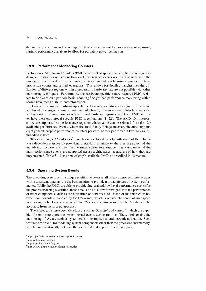
Tools such as perf 6 and PAPI7 have been developed to help with some of these hard-ware dependence issues by providing a standard interface to the user regardless of theunderlying microarchitecture. While microarchitecture support may vary, many of themain performance events are supported across architectures, regardless of how they areimplemented. Table 5.1 lists some of perf ’s available PMCs as described in its manual.

5.3.4 Operating System Events

The operating system is in a unique position to oversee all of the component interactionswithin a system, placing it in the best position to provide a broad picture of system perfor-mance. While the PMCs are able to provide fine-grained, low level performance events forthe processor during execution, these details do not allow for insights into the performanceof other components, such as the hard drive or network card. Much of the interaction be-tween components is handled by the OS kernel, which is outside the scope of user-spacemonitoring tools. However, some of the OS events require kernel patches/modules to beaccecible from the user perspective.

Therefore, tools have been developed, such as Oprofile8 and netatop9, which are capa-ble of monitoring operating system kernel events during runtime. These tools enable themonitoring of events, such as system calls, interrupts, bus and network utilization. Suchfeatures are crucial for modeling system components other than the processor and memory,which have traditionally not been the focus of detailed performance analysis.

6https://perf.wiki.kernel.org/index.php/Main Page7http://icl.cs.utk.edu/papi/8http://oprofile.sourceforge.net9http://www.atoptool.nl/downloadnetatop.php

INTERACTION BETWEEN POWER AND PERFORMANCE 15

Table 5.1 Some of the hardware performance counters available in perf.

Name Description

cpu-cycles Total cycles (affected by CPU frequency scaling).

instructions Retired instructions.

branch-instructions Retired branch instructions.

branch-misses Mispredicted branch instructions.

bus-cycles Bus cycles, which can be different from total cycles.

idle-cycles-frontend Stalled cycles during issue.

idle-cycles-backend Stalled cycles during retirement.

ref-cycles Total cycles (not affected by CPU frequency scaling).

L1-dcache-(loads/stores/prefetches) Level 1 Data cache read/write/prefetch accesses.

L1-dcache-(loads/stores/prefetches)-misses Level 1 Data cache read/write/prefetch misses.

LLC-(loads/stores/prefetches) Last Level Cache read/write/prefetch accesses.

LLC-(loads/stores/prefetches)-misses Last Level Cache read/write/prefetch misses.

iTLB-loads Instruction TLB read accesses.

iTLB-load-misses Instruction TLB read misses.

node-(loads/stores) Local memory read/write accesses.

node-loads-misses Local memory read misses.

5.3.5 Virtual Machine Performance

Virtualized environments present a challenging problem for performance monitoring. Even-though some PMC can be accessed from the host (physical) machine for some virtualiza-tion software, such as VMware and KVM; the guest virtual machines (VMs) do not havedirect access to the underlying hardware. This may prevent the use of some previouslydiscussed profiling techniques. For instance, Xen does not virtualize the PMC registersdue to the significant performance cost that would be incurred, preventing the use of toolslike perf and Oprofile in the guest machine.

Tools such as Xenoprof 10 instrument the hypervisor and the guest OS to enable the mon-itoring of PMCs within the hypervisor, which are then matched to the guests’ operations.Since Xenoprof is an extension of Oprofile, it is capable of providing similar performanceanalysis functionality. Recent versions of KVM and Qemu also support PMC in the guestOS.

5.4 Interaction between Power and Performance

While the performance characteristics of key system components are generally well un-derstood, the corresponding power characteristics remain less so. This can largely be at-tributed to differences in component interactions, where performance is often consideredindependent, power has many flow-on effects, creating interdependencies between compo-

10http://xenoprof.sourceforge.net/

16 POWER MODELING

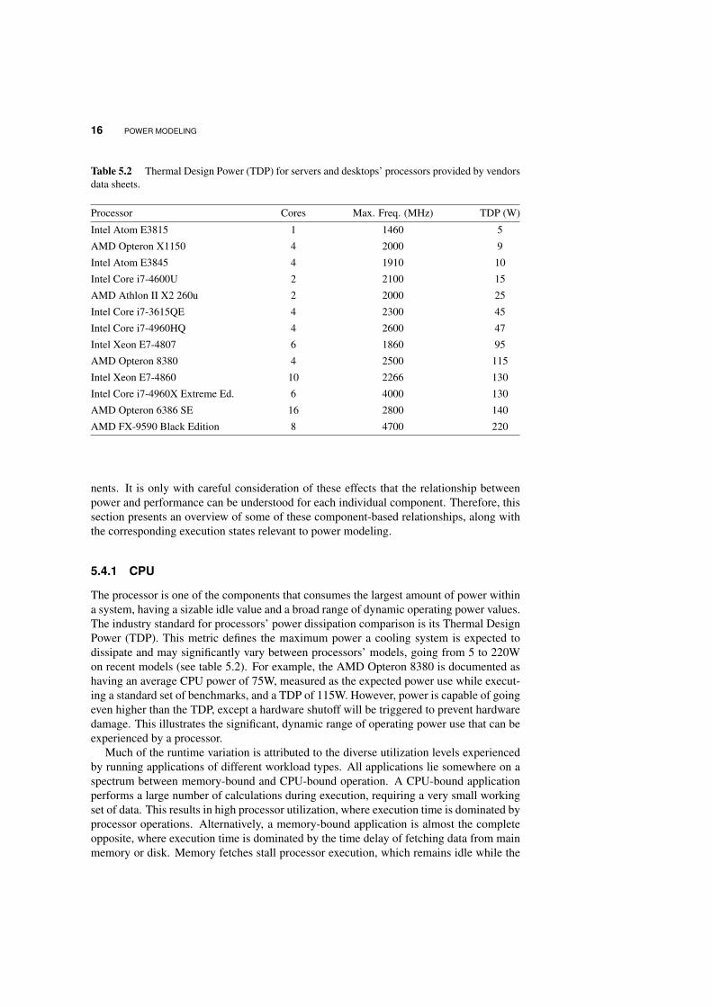
Table 5.2 Thermal Design Power (TDP) for servers and desktops’ processors provided by vendorsdata sheets.

Processor Cores Max. Freq. (MHz) TDP (W)

Intel Atom E3815 1 1460 5

AMD Opteron X1150 4 2000 9

Intel Atom E3845 4 1910 10

Intel Core i7-4600U 2 2100 15

AMD Athlon II X2 260u 2 2000 25

Intel Core i7-3615QE 4 2300 45

Intel Core i7-4960HQ 4 2600 47

Intel Xeon E7-4807 6 1860 95

AMD Opteron 8380 4 2500 115

Intel Xeon E7-4860 10 2266 130

Intel Core i7-4960X Extreme Ed. 6 4000 130

AMD Opteron 6386 SE 16 2800 140

AMD FX-9590 Black Edition 8 4700 220

nents. It is only with careful consideration of these effects that the relationship betweenpower and performance can be understood for each individual component. Therefore, thissection presents an overview of some of these component-based relationships, along withthe corresponding execution states relevant to power modeling.

5.4.1 CPU

The processor is one of the components that consumes the largest amount of power withina system, having a sizable idle value and a broad range of dynamic operating power values.The industry standard for processors’ power dissipation comparison is its Thermal DesignPower (TDP). This metric defines the maximum power a cooling system is expected todissipate and may significantly vary between processors’ models, going from 5 to 220Won recent models (see table 5.2). For example, the AMD Opteron 8380 is documented ashaving an average CPU power of 75W, measured as the expected power use while execut-ing a standard set of benchmarks, and a TDP of 115W. However, power is capable of goingeven higher than the TDP, except a hardware shutoff will be triggered to prevent hardwaredamage. This illustrates the significant, dynamic range of operating power use that can beexperienced by a processor.

Much of the runtime variation is attributed to the diverse utilization levels experiencedby running applications of different workload types. All applications lie somewhere on aspectrum between memory-bound and CPU-bound operation. A CPU-bound applicationperforms a large number of calculations during execution, requiring a very small workingset of data. This results in high processor utilization, where execution time is dominated byprocessor operations. Alternatively, a memory-bound application is almost the completeopposite, where execution time is dominated by the time delay of fetching data from mainmemory or disk. Memory fetches stall processor execution, which remains idle while the


data is retrieved. This results in few calculations been performed, and a correspondinglylow processor utilization.

This variation in workload utilization characteristics has been leveraged by the mostprevalent power saving policies in modern operating systems. Power is saved by adjust-ing the processors’ operating frequency at runtime using DVFS, so that it is ideally setproportionally to the memory-boundedness of an application. Using a low operating fre-quency will slow the rate of processor operations, increasing execution time for computetasks while saving power. Since only processor operations are impacted, a memory-boundworkload will experience minimal performance degradation as the memory access latencyis not affected. However, running a CPU-bound workload at a low frequency will sacrificea great deal of performance. Many alternate policies have been implemented to evaluatethe tradeoff between power and performance, attempting a maximizing savings withoutimpacting performance. Figure 5.1 shows the power dissipated by a machine equippedwith an Intel Core i7-3615QE processor while running Linux’s CPU stress benchmark atall available frequencies.

1.2 1.3 1.4 1.5 1.6 1.7 1.8 1.9 2.0 2.1 2.2 2.3

86

88

90

92

94

96

Stressed CPU

Frequency (GHz)

Pow

er

(W)

Figure 5.1 Power dissipated by a Intel(R) Core(TM) i7-3615QE CPU machine while running thesame workload on different frequencies.

Unfortunately, such policies do not allow for any power savings while executing CPU-bound applications, resulting in high power consumption. To achieve such savings, manu-facturers have implemented fine-grained, low-level power saving techniques in hardware,namely Cstates. Aggressive clock gating is used to switch off parts of the microproces-

18 POWER MODELING

sor’s circuity, temporarily suspending functional units, where state is maintained by stop-ping flip-flops. Reasonable power savings may be made with the ever increasing densityof processors and number of functional units. However, this essentially creates a hiddenpower state, strictly controlled in hardware, that the operating system is not able to observe.This raises new challenges for modeling power, although if enough fine-grained details areknown about the current application workload, the processor’s functional unit state couldpotentially be inferred by the expected unit utilization.

While the processor consumes a large amount of power, it is worth remembering thatsome of the observed consumption may be due to flow-on effects from other system com-ponents. The most straightforward illustration of this is the power use of system fans. Asthe processor’s utilization increases, the temperatures generated increase, causing the cool-ing system to use more power. However, this relationship is complicated by the thermalchanges occurring at a slower rate than the corresponding changes in utilization, as wasobserved in [38]. Such cross-component power dependencies are more significant for theprocessor than any other system component, given the central role played in all systemoperations.

5.4.2 Memory

The interdependence of processor and memory power consumption was indirectly shownin the previous section, where memory-bound workloads stall execution, lowering utiliza-tion and power consumption of the processor. However, the power reduction in the pro-cessor cannot be easily isolated from any potential increase in power use from the memorymodules due the changes occurring simultaneously.

This can lead to the actual power use of memory modules been obscured, causing erro-neous conclusions to be drawn as to the significance of power use. For instance, memoryis sometimes thought to consume a sizable amount of power, but the specifications forKingston hyperx memory shows a power draw of only 0.795W11 while operating. A typ-ical system may contain about eight memory modules, giving a total of 6.36W, which isalmost insignificant in the context of other system components.

Observed changes in power consumption for a memory dominated workload can mostlikely be attributed to cross-component power dependencies, where the memory modulesthemselves have minimal impact. Instead power reduction comes from lower processorutilization, given that a new task is not switched onto the processor, which will have thefurther flow-on effect of reducing temperatures.

5.4.3 I/O

A certain percentage of memory accesses will result in pages being fetched from the harddisk, incurring additional processor latency as data transfers are significantly slower thanthe processor’s operating speed. However, any large data transfers will be handled bya direct memory access (DMA) operation, allowing the processor to continue executionwhile transfers proceed independently.

As a result, the processor will not be aware of the hard disk’s operating state at any giventime. Therefore, hard disk utilization levels can only be monitored from the operatingsystem, which is able to track the interrupts used to handle the transfer, in addition to busutilization levels.

11http://www.valueram.com/datasheets/khx1600c8d3t1k2 4gx.pdf


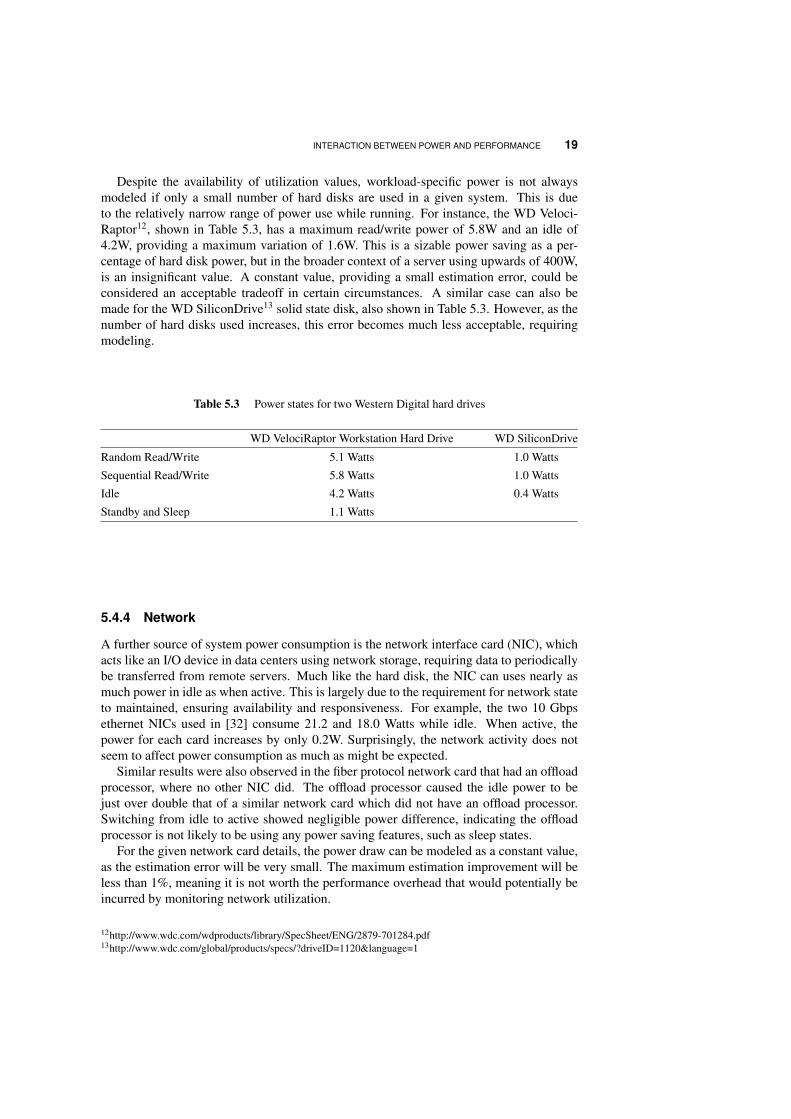
Despite the availability of utilization values, workload-specific power is not alwaysmodeled if only a small number of hard disks are used in a given system. This is dueto the relatively narrow range of power use while running. For instance, the WD Veloci-Raptor12, shown in Table 5.3, has a maximum read/write power of 5.8W and an idle of4.2W, providing a maximum variation of 1.6W. This is a sizable power saving as a per-centage of hard disk power, but in the broader context of a server using upwards of 400W,is an insignificant value. A constant value, providing a small estimation error, could beconsidered an acceptable tradeoff in certain circumstances. A similar case can also bemade for the WD SiliconDrive13 solid state disk, also shown in Table 5.3. However, as thenumber of hard disks used increases, this error becomes much less acceptable, requiringmodeling.

Table 5.3 Power states for two Western Digital hard drives

WD VelociRaptor Workstation Hard Drive WD SiliconDrive

Random Read/Write 5.1 Watts 1.0 Watts

Sequential Read/Write 5.8 Watts 1.0 Watts

Idle 4.2 Watts 0.4 Watts

Standby and Sleep 1.1 Watts

5.4.4 Network

A further source of system power consumption is the network interface card (NIC), whichacts like an I/O device in data centers using network storage, requiring data to periodicallybe transferred from remote servers. Much like the hard disk, the NIC can uses nearly asmuch power in idle as when active. This is largely due to the requirement for network stateto maintained, ensuring availability and responsiveness. For example, the two 10 Gbpsethernet NICs used in [32] consume 21.2 and 18.0 Watts while idle. When active, thepower for each card increases by only 0.2W. Surprisingly, the network activity does notseem to affect power consumption as much as might be expected.

Similar results were also observed in the fiber protocol network card that had an offloadprocessor, where no other NIC did. The offload processor caused the idle power to bejust over double that of a similar network card which did not have an offload processor.Switching from idle to active showed negligible power difference, indicating the offloadprocessor is not likely to be using any power saving features, such as sleep states.

For the given network card details, the power draw can be modeled as a constant value,as the estimation error will be very small. The maximum estimation improvement will beless than 1%, meaning it is not worth the performance overhead that would potentially beincurred by monitoring network utilization.

12http://www.wdc.com/wdproducts/library/SpecSheet/ENG/2879-701284.pdf13http://www.wdc.com/global/products/specs/?driveID=1120&language=1

20 POWER MODELING

5.4.5 Idle states

Power models seek to model the power response in components for various utilizationlevels. However, one utilization level which is often not explicitly modeled [31], is thebase power while the system is idle. This is important because in many large-scale serverdeployments, a significant proportion of time is spent idle [2]. If a model does not incor-porate these workload phases, then the model will begin to diverge from real world poweruse over long periods of operation.

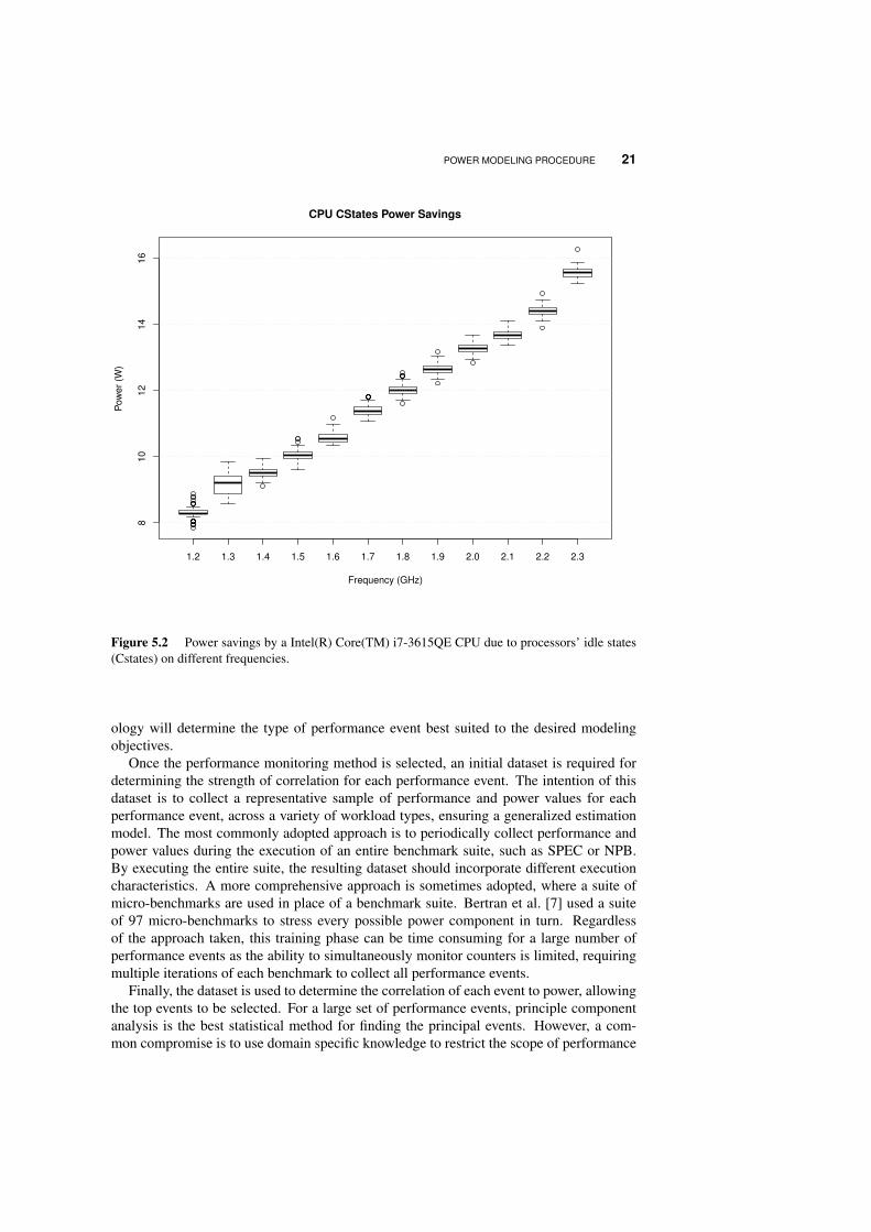
Power models essentially estimate the dynamic response in power for a correspondingchange in utilization, specifically the dynamic power of a system. Therefore, the systempower, which does not change with utilization is considered static power, representing thebase power for the system and components. The static power includes many unmodeledsystem components, such as the power supply unit or motherboard chipset. At a finergranularity, it can also be thought of including the base power for many of the ‘dynamic’components. For instance, the processor consists of both static and dynamic power, wheredynamic power is the utilization response and static power is the persistent base power forthe component. Figure 5.2 presents the power savings due to the use of these techiniqueson a Intel Core i7-3615QE. Considering that its TDP is 45W (table 5.2), these savingscan achieve up to 33% of processors’ TDP. Furthermore, it will be shown in the modelevaluation section, that not making this distinction between what is and is not modeled hasthe potential to misrepresent the accuracy of estimations.

In summary, different workload types will keep different components busy in the systemand therefore incur different power usage patterns. This observation is crucial for buildingpower estimation models based on system events.

5.5 Power Modeling Procedure

The process of deriving a power model, capable of providing accurate runtime power es-timates, without the need for special purpose hardware metering, can be broken down tofour steps: (1) variable selection, (2) training data acquisition, (3) model construction, and(4) model evaluation. The process followed during each stage of development will ulti-mately determine the generality and accuracy of the resulting model. In this section, eachstep is independently discussed, providing general guidance, that can be used to createimplementations in a variety of system environments.

5.5.1 Variable Selection

The first step in deriving a power estimation model is the selection of performance eventsthat strongly correlate with power, namely Key Performance Indicators (KPI), for a diverseset of workloads. The available performance events are largely dictated by the chosenmodeling methodology and systems execution environment.

For instance, many modeling methodologies restrict performance monitoring to the pro-cessor and memory modules, given their dominance of both execution performance andpower consumption. In such cases, fine-grained performance events are desired, resultingin the selection of PMCs for their ability to monitor low-level events. This in turn imposesa limit on the number of events able to be monitored simultaneously, due to the microar-chitecture dependence of the chosen approach. Alternatively, including network and I/Ocomponents in the modeling methodology requires the use of kernel performance events,possibly in addition to PMCs. Therefore, the initial specification of modeling method-

POWER MODELING PROCEDURE 21

1.2 1.3 1.4 1.5 1.6 1.7 1.8 1.9 2.0 2.1 2.2 2.3

810

12

14

16

CPU CStates Power Savings

Frequency (GHz)

Pow

er

(W)

Figure 5.2 Power savings by a Intel(R) Core(TM) i7-3615QE CPU due to processors’ idle states(Cstates) on different frequencies.

ology will determine the type of performance event best suited to the desired modelingobjectives.

Once the performance monitoring method is selected, an initial dataset is required fordetermining the strength of correlation for each performance event. The intention of thisdataset is to collect a representative sample of performance and power values for eachperformance event, across a variety of workload types, ensuring a generalized estimationmodel. The most commonly adopted approach is to periodically collect performance andpower values during the execution of an entire benchmark suite, such as SPEC or NPB.By executing the entire suite, the resulting dataset should incorporate different executioncharacteristics. A more comprehensive approach is sometimes adopted, where a suite ofmicro-benchmarks are used in place of a benchmark suite. Bertran et al. [7] used a suiteof 97 micro-benchmarks to stress every possible power component in turn. Regardlessof the approach taken, this training phase can be time consuming for a large number ofperformance events as the ability to simultaneously monitor counters is limited, requiringmultiple iterations of each benchmark to collect all performance events.

Finally, the dataset is used to determine the correlation of each event to power, allowingthe top events to be selected. For a large set of performance events, principle componentanalysis is the best statistical method for finding the principal events. However, a com-mon compromise is to use domain specific knowledge to restrict the scope of performance

22 POWER MODELING

events to key units of interest. For example, Singh et al. [31] decomposed the processor andmemory into four categories, considered the most significant functional units: FPU, mem-ory accesses, processor stalls and instructions retired. Consequently, only 13 PMCs neededto be collected for the dataset, with a single, strongly correlated event being selected to rep-resent each category. Such a small dataset facilitated simpler, manual correlation methods.

5.5.2 Training Data Collection

While the benchmarks used for event selection provide a representative sample of workloadtypes and utilization levels, they are not guaranteed to represent an exhaustive set of pos-sible values. For a power model to be widely deployable, it needs be capable of accuratelyestimating the power of previously unseen workloads, requiring benchmark independence.Therefore, micro-benchmarks are exclusively used for collecting model training data.

A specific micro-benchmark is created for each of the selected performance events,with each being configured to explore a diverse spread of performance values. If micro-benchmarks were used for event selection, those corresponding to the selected events canbe reconfigured and reused for collecting the model training data. By replicating perfor-mance events beyond typical ranges, the resulting model will be more capable of accuratelyestimating power for less commonly seen applications. However, this requires a tradeoffto be made between accuracy and training time, as a significant number of execution con-figurations exist. A commonly used compromise is to explore a select sample of boundarycases, while spending the majority of training time within typical ranges.

5.5.3 Learning from Data

The most commonly used approach for modeling power is to derive a linear regressionmodel from a training set of key performance indicators (KPI)/power observations. Train-ing data is periodically collected as a series of tuples, 〈power ,KPI 1, . . . ,KPI n〉, wherethe resulting accuracy of the model will depend on how well the training data representsthe expected workload type for power estimation. For the regression model, power is thedependent variable estimated by the explanatory performance values.

Let y be a vector of n power measurements (observations) from the training dataset

y = [y1, y2, . . . , yn] , (5.1)

where n is the total number of tuples in the dataset. The performance events are the inde-pendent variables used for predicting power, defining a Xn×m matrix, where each matrixline is described as

xi = [xi,1, xi,2, . . . , xi,m] i ∈ {1, . . . , n}, (5.2)

where xi is a vector of m key performance event measurements taken at time ti. Thisforms the linear regression model:

yi = β0 +

m∑j=1

βjφjxi,j + ξi, (5.3)


where ξi is the measurement error and φ1, . . . , φm are non-linear functions. The β coeffi-cient parameters can be estimated by calculating the least squares

S =

n∑i=1

yi − β0 − m∑j=1

βjφjxi,j

2

, (5.4)

which minimizes the sum of the squared errors for all of the coefficients.The resulting regression coefficients, β0, . . . , βm, are used to form the power estimation

model, where the runtime measurements of performance event are used as input parame-ters to the model to estimate the dependent power value. This determines the analyticalrelationship between a set of key performance events and power. The accuracy of the re-sulting model will depend on many factors, including the selection of performance events,which will be discussed in more detail throughout this chapter.

5.5.3.1 Alternative Modeling Methods A variety of alternate approaches to powermodeling have previously been proposed, varying in the selection of performance eventsand the correlation methods. Many of the early models were formed by the observed re-lationship between system utilization, typically measured as instructions per cycle (IPC),and power [37]. Essentially, only the processor power is modeled, but a reasonable esti-mation accuracy was able to be reached. This was due in a large part to the dominance ofprocessor power in the simple, single-core system.

Mantis [16] extended the relationship between utilization and power to other systemcomponents, deriving a power model for the entire system by incorporating memory, harddisk and network performance in addition to processor utilization. The selected perfor-mance events come from hardware Performance Monitoring Counters (PMCs) and OSperformance events: CPU utilization, off-chip memory access counters, hard disk I/O rateand network I/O rate. The power model is derived from an initial, one-time calibrationphase in which benchmarks are run to stress each of these system components in turn,while recording the power from each AC line. A linear program is then used to derivethe power model by minimizing the estimation error across all performance events with alinear function. However, the model’s accuracy relies on the calibration phase providing arange of utilization levels that are representative of realistic workloads, and not merely thescientific workloads used for model evaluation.

More refined power models are possible by modeling sub-components instead of aggre-gate component utilization levels. Bellosa [5] noted a strong linear relationship betweenfour synthetic workloads designed to stress individual processor functional units, four log-ically correlated low-level performance events and power. The four performance eventswere: processor micro-uops, FLOPS, l2-cache misses and memory transactions. By isolat-ing the power draw of each low-level function, the linear models were able to be combinedinto a single power model, Joule Watcher.

A similarly fine-grained, processor based, power model was proposed by Singh et al.in [31], which used domain specific knowledge to decompose the processor into four keyfunctional units. A single, strongly correlated PMC was found for each functional unit.Event-specific micro-benchmarks were designed to stress the breadth of potential oper-ating values, taking care to include some extreme outliers. Through this exploration of alarge utilization space, it was observed that some performance events experienced differentpower characteristics at low levels than at high levels, which can only be modeled with anon-linear function. The model was further improved through the use of a piecewise linearfunction, separating the low event values from high, allowing subtly more complex event

24 POWER MODELING

characteristics to be modeled. However, the improvements provided were not explicitlyevaluated, merely the accuracy of the resulting model.

The increasing complexity of processor hardware has raised some concerns that linearmodels may not be sufficiently complex to accurately model power anymore. In fact, theseconcerns are not new but merely an extension of the ongoing debate regarding the requiredtrade off between model complexity and accuracy. A marginally more complex model wasproposed by Bircher et al. [8] where the key subsystems are modeled independently using aquadratic function. The five key subsystems modeled are: CPU, memory, chipset, I/O anddisk. The power for each subsystem is determined during an initial training period by plac-ing resistors in series with the power supply, making it a significantly more complicatedprocedure than the other approaches discussed so far. After the power for each compo-nent is isolated, a series of benchmarks are run, stressing each subsystems in turn. Theresulting model uses processor-centric performance events, all PMCs with the exceptionof interrupt counters, to model all of the components. This is a rather unique approach, asmany of the previous systems rely on operating system events to monitor utilization levelsfor components such as the hard disk. Instead, the processor PMCs are used to analyze the“trickle-down” effect of processor events through other system components. For instance,a last-level cache miss will cause a memory access, which may in turn cause a disk access.Monitoring these effects allowed the subsystem components to be modeled using only sixperformance events, with an average error of less than 9% per subsystem.

A potential problem with using general utilization metrics, like IPC, is that they provideinsufficient detail to adequately distinguish between various workload types. This was ob-served by Dhiman et al. [13] when executing a series of benchmarks in a range of alternateconfigurations, which resulted in different levels of power use for similar utilization levels.Therefore, the authors propose a modeling technique based upon a rudimentary clusteringof workload types using a Gaussian Mixture Model (GMM), with four input performancecounters: instructions per cycle (IPC), memory accesses per cycle (MPC), cache trans-actions per cycle (CTPC) and CPU utilization. The resulting power model was able tooutperform two simple, alternative regression-based models during evaluation.

These are but a select few of the wide variety of power modeling methodologies tohave previously been proposed. Alternate methodologies differ in the approach taken forperformance event selection, collection of training data, modeled system components andthe regression method used to derive the power model. Consequently, the remainder of thischapter attempts to remain implementation independent by discussing all relevant conceptsat a high-level whenever possible.

5.5.4 Event Correlation

The power model is constructed by quantifying the relationship between the selected per-formance events and power for an extensive model training dataset. In the model, per-formance events provide the explanatory variables used to predict the dependent powervariable. This arrangement lends itself well to the use of regression techniques to form anestimation model. One of the simplest, and most readily applied regression techniques isto derive a series of per-component regression models, combined into a single model:

power = XCPU +Xmemory +XI/O + ξ (5.5)

While such a model is easily understood, given the prevalence of component-specificperformance events, the previously discussed impact of cross-component effects is largelyneglected. The use of an error term may mitigate some of the impact, but does not resolve


the underlying problem, with the model’s simplicity sacrificing accuracy. Support vectorregression provides a more robust regression method by fitting a single, non-linear functionto a small training dataset. This approach was used in [35].

The accuracy of simple regression models is limited by the use of a single fitting func-tion, required to adequately represent the execution characteristics of widely varying uti-lization levels and workload types. The resulting estimation model may become overlygeneral, where a more accurate fit could be achieved by characterizing utilization. Thevariation in high and low utilization behavior was noted by Singh et al. [31]. To rectifythese differences, a piecewise regression model was proposed, enabling different estima-tion functions to be used at each of the utilization levels.

The improvements provided by workload characterization can be further extended byusing a workload classification scheme. By classifying execution workloads, a separateregression model can be derived for each source of a dominant workload. For instance,most derived models are processor centric, achieving good estimation accuracy for pro-cessor dominated workloads. However, the accuracy can be significantly worse for otherworkloads, such as memory-bound applications, due to the model’s bias towards processorpower. Enabling the model to tailor power estimates to a given workload helps to removemuch of this bias by using the most appropriate estimation function at the appropriatetime. Such an approach was taken in Dhiman et al. [13], where it was observed that sim-ilar utilization levels often resulted in different power consumption for various workloadtypes. Classification allowed each workload to be treated separately, improving the overallestimation accuracy.

5.5.5 Model Evaluation Concepts

Power models are evaluated by assessing the effectiveness of power estimates for a suite ofbenchmarks. For a fair evaluation, the chosen benchmark suite should not be the same aswas used during event selection, but should similarly consist of a diverse set of workloadtypes. This helps determine how well a given model will generalize across various utiliza-tion levels, as a poorly selected set of performance events and training dataset may containbias towards a specific workload.

5.5.5.1 Statistical Metrics Summary statistics like the median error are commonly usedto present the evaluation error of the estimation model, but this has the potential to mis-represent the accuracy of the model. This is primarily due to the selection of evaluationbenchmarks, which are typically scientific workloads, and their dominance of a singleexecution phase. For example, a compute intensive benchmark will spend much of its ex-ecution time in high utilization phases, with a significantly smaller portion of executiontime spent executing memory-bound tasks, such as reading/writing log files. As a result,a power estimation model will achieve a low median error overall if it is able to closelyestimate the dominant execution phase—compute intensive work—given its dominance.Therefore the median error is not affected by the other execution phases, making it a poormetric to gauge the quality of fit for all execution phases.

Alternatively, the mean absolute error (MAE) provides the mean estimation error for allexecution phases, and will thus be negatively impacted by any significant outliers causedby poor estimation during non-dominant phases. However, this only solves part of theproblem, as a single metric, such as the mean absolute or median error, is not capable ofproviding a meaningful description of total execution accuracy. They can only providecursory insights. More detail can easily be provided by additionally including the standard

26 POWER MODELING

deviation, which describes the spread of estimation values from the mean over the entireexecution.

5.5.5.2 Static versus Dynamic power The importance of the distinction between staticand dynamic power was previously discussed, which is an important consideration to bemade when evaluating power estimation. The most important takeaway is that a powermodel is essentially only estimating the dynamic power of a system. That is the responsein power consumption to a corresponding change in performance events or utilization. Pre-senting the estimation error as a percentage of the system’s dynamic power—that is actu-ally being estimated—allows for fairer comparisons to be made between different models,developed on different systems. An example of this was given in [38]:

For example, suppose there are two different power models with identical mean esti-mation errors of 5%, but for different machines with an equal total power consumptionof 200W. Without further information, the initial conclusion that can be drawn by thereader is both power models are equally accurate. However, a different conclusion can bedrawn if it was additionally known that machine ‘A’ has a dynamic power (aka workloaddependent power) of 30%, while machine ‘B’ has a larger dynamic power of 60%. Givena total error of 10W (5% of total 200W) and the constant static power (aka base power),it is now clear that the model based on machine ‘A’ has a 16.6% error for dynamic powerwhile the model based on machine ‘B’ has a much lower error of 8.3% for dynamic power.The extra information on the proportion of static power and dynamic power enables a faircomparison to be made between the two, otherwise apparently identical power estimationmodels.

Results can appear misleading or lead to erroneous conclusions if they are not presentedin the fairest way possible. Furthermore, the actual accuracy of an estimation model canpotentially be obscured by the relative static and dynamic power values on systems witha relatively small dynamic power range as a proportion of total power. Such cases aremore likely on systems that use low-power components, which can have minimal operatingranges.

5.5.6 Model Evaluation

While it is desirable to achieve perfect power estimation, such an objective may be unob-tainable in practice. Such attempts may incur significant runtime overhead, where a lessaccurate, but more efficient power model, may prove to be sufficient for most use-cases.

5.5.6.1 Estimation errors In modeling hardware component power consumption, atradeoff between model complexity and accuracy is required. This problem is exacer-bated by the increasing complexity of newer microarchitectures, which can be attributed tothe incorporation of: hardware threading, fine-grained power saving modes, and increas-ing component densities. Therefore, estimation models must approximate many of thesepower factors, balancing runtime performance monitoring and model complexity with es-timation accuracy. Collecting a large number of performance events, and modeling all ofthe corresponding interactions reaches a point where it becomes more akin to simulation,with gains in accuracy being outweighed by the runtime overhead.

Fortunately, if appropriate care is taken while deriving the model, many sources of ap-proximation can be controlled for, or incorporated into the model. For instance, Mair etal. [39] noted that the version of compiler used or the compiler optimization level, impactsa benchmarks power characteristics. Such variations could be incorporated into the model


by treating alternative compiler/benchmark configurations as separate benchmarks usedduring training, instead of a single benchmark run multiple times. Temperature is anothercommonly considered factor influencing power consumption, which can be difficult toreliably measure. This is primarily due to the poor quality of standard measurement equip-ment and significant latencies in observable thermal effects within a system. A simple,but apparently rarely considered, approach to mitigating some of the impact is to ensurethat execution times are sufficiently long so that a stable operating temperature is reachedbefore data collection. Short, periodic executions can lead to below-average power usefor a given workload, as the temperature will be below the typical operating point giveninsufficient time for processor warm-up. These two factors, among others, illustrate theimportance of taking care in setting up a model’s experimental configuration.

However, some sources of estimation error are beyond measurement and are unableto be incorporated into the model. The most common source of these errors is hardwarepower saving features that operate independently of the operating system, and are thereforetransparent to the system. The best example of this, which was previously mentioned, is theanecdotal evidence of aggressive clock gating in modern processors [26], where functionalunits within the processor are shut off while inactive, in order to save power. Given the lackof understanding as to how this feature operates, it is even difficult to trigger the occurrenceof certain actions during model training in an attempt to incorporate the respective powervariations. A further source of inconsistent hardware power measurements may be due tomanufacturing variability. An experiment in [26] observed an 11% difference in powerbetween two Intel Core i5-540M processors, in the same experimental configuration.Thiscan exacerbate estimation errors where a model is trained on one processor and is used onother processors, thought to be identical. This illustrates the unlikely nature of eliminatingall sources of estimation error. Therefore, the question should be, what is an acceptableestimation error?

5.5.6.2 An Acceptable Error There is no single criteria for determining if a given powerestimation model is accurate enough, as each use case will have different tolerances ofestimation errors. For instance, using the power model to evaluate how best to consolidateworkloads in a datacenter has a rather high tolerance, suggested to be 5-10% by [26], dueto the coarse-grained nature of per-server power estimation. Alternatively, if the samedatacenter were to use this model to charge clients for the power each submitted job usesduring execution, an error this high for the entire system would not be tolerated. Such ahigh error would possibly lead to charging clients for resources not actually used.

The most commonly proposed use for power models is in making power-aware taskschedulers. Power-aware task scheduling is a rather generic term, giving rise to many dif-ferent scheduling policies. For the discussion here, we define “power-aware task schedul-ing” as using a scheduler that prioritizes resource allocation to the most power efficientuses, while maintaining all strict resource requirements and workload deadlines. For in-stance, to determine which task should be allocated additional processor cores, the powermodel can be used to determine the change in power in response to a given allocation. Thepower efficiency for each task is then evaluated as the size of the relative power change,thereby indicating which task will use the least additional power. A fair evaluation has twoaccuracy requirements. First, the estimation error needs to remain stable across workloadsto prevent any bias in evaluation. Second, the estimation error needs to be less than thepower difference of any two cores, otherwise the error may hide the real change in power.These requirements mean the allowable estimation error will be system specific, as differ-ent architectures will have processors with significantly varying operating ranges for power

28 POWER MODELING

use. Unfortunately, this means that no single rule exists for determining a specific thresh-old for modeling accuracy. However, the simple fact remains, the greater the estimationaccuracy, the better.

5.6 Use Cases

Power estimators can be used on several perspectives. This section presents some of itsapplications focusing on three possible kinds of users: end-users, software developers andsystem managers. These usage perspectives provide the motivational background for thecreation of power estimators which differ according to the machine’s architecture. Here wedivide the power modeling methodology based on single core, multicore and distributedsystems, summarizing some implementations and their accuracy.

5.6.1 Applications

Depending on the interest/knowledge of the user, the power dissipated by an applica-tion/machine may be differently exploited. If we consider the end-user, i.e. a person whointeracts with the system without bothering about implementation details, such estimatorsmay provide a user feedback on how much power is dissipated by the system while execut-ing some programs, increasing the awareness of use impact. This can be achieved either apriori, using energy efficiency labels, or at execution time, providing an energy per processmonitoring solution. While the former faces some disagreement on how the labels shouldbe created, the latter method is already used, mainly by the operating systems of portabledevices.

For software developers, hardware’s usage deeply depends on how the application isimplemented. The impact of an application over its dissipated power includes the librariesthat it uses, its coding patterns and the compilers employed. In [29], the authors com-pare the impact of compiling a similar code using different compilers and programminglanguages on its overall energy consumption. They used different implementations of theTower of Hanoi solver and compared their energy spent to solve the same problem size.The codes were written by different authors and their expertise on the programming lan-guages are not taken into account in the evaluation. A similar approach can be done toselect which compilation flags and libraries given software may use.

Possibly, due to its highest energy consumption, the system manager is the one whomay have the major benefits. The possibility of monitoring applications’ power usage maylead to new resource managing policies on different levels. In [36], the authors exploit theenergy as a resource on Linux systems, proposing kernel level allocation policies. Someportable OS, such as Google’s Android and Apple’s iOS, also monitor applications’ poweruse and the battery status can define if software may or may not be launched. At the datacenter level, the resource allocation and job scheduler can use such information to turnnodes on or off.

5.6.2 Single core systems

Single core systems are the easiest on which to implement the previously explained meth-ods. On such systems, as there is only a single flow of execution, it is simpler to takethe necessary measurements. Indeed, there is only one subject as the core is the sameas the processor and as the node. It is then possible to correlate measurements from the

USE CASES 29

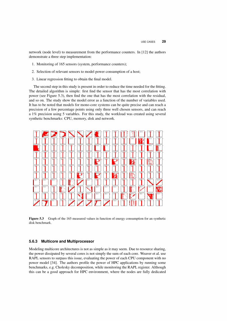
network (node level) to measurement from the performance counters. In [12] the authorsdemonstrate a three step implementation:

1. Monitoring of 165 sensors (system, performance counters);

2. Selection of relevant sensors to model power consumption of a host;

3. Linear regression fitting to obtain the final model.

The second step in this study is present in order to reduce the time needed for the fitting.The detailed algorithm is simple: first find the sensor that has the most correlation withpower (see Figure 5.3), then find the one that has the most correlation with the residual,and so on. The study show the model error as a function of the number of variables used.It has to be noted that models for mono-core systems can be quite precise and can reach aprecision of a few percentage points using only three well chosen sensors, and can reacha 1% precision using 5 variables. For this study, the workload was created using severalsynthetic benchmarks: CPU, memory, disk and network.

3:2 4:2 5:2 6:2 7:2 8:2 9:2 10:2 11:2 12:2 13:2 14:2 15:2 16:2 17:2

18:2 19:2 20:2 21:2 22:2 23:2 24:2 25:2 26:2 27:2 28:2 29:2 30:2 31:2 32:2

33:2 34:2 35:2 36:2 37:2 38:2 39:2 40:2 41:2 42:2 43:2 44:2 45:2 46:2 47:2

48:2 49:2 50:2 51:2 52:2 53:2 54:2 55:2 56:2 57:2 58:2 59:2 60:2 61:2 62:2

63:2 64:2 65:2 66:2 67:2 68:2 69:2 70:2 71:2 72:2 73:2 74:2 75:2 76:2 77:2

78:2 79:2 80:2 81:2 82:2 83:2 84:2 85:2 86:2 87:2 88:2 89:2 90:2 91:2 92:2

93:2 94:2 95:2 96:2 97:2 98:2 99:2 100:2 101:2 102:2 103:2 104:2 105:2 106:2 107:2

108:2 109:2 110:2 111:2 112:2 113:2 114:2 115:2 116:2 117:2 118:2 119:2 120:2 121:2 122:2

123:2 124:2 125:2 126:2 127:2 128:2 129:2 130:2 131:2 132:2 133:2 134:2 135:2 136:2 137:2

138:2 139:2 140:2 141:2 142:2 143:2 144:2 145:2 146:2 147:2 148:2 149:2 150:2 151:2 152:2

153:2 154:2 155:2 156:2 157:2 158:2 159:2 160:2 161:2 162:2 163:2 164:2 165:2 166:2 167:2

Figure 5.3 Graph of the 165 measured values in function of energy consumption for an syntheticdisk benchmark.

5.6.3 Multicore and Multiprocessor

Modeling multicore architectures is not as simple as it may seem. Due to resource sharing,the power dissipated by several cores is not simply the sum of each core. Weaver et al. useRAPL sensors to surpass this issue, evaluating the power of each CPU component with nopower model [34]. The authors profile the power of HPC applications by running somebenchmarks, e.g. Cholesky decomposition, while monitoring the RAPL register. Althoughthis can be a good approach for HPC environment, where the nodes are fully dedicated

30 POWER MODELING

to execute one application at a time, it can only be used on some generations of Intelprocessors.

Basmadjian and Meer address this issue by modeling each CPU component [4]. Thesecomponents are stressed at different levels through the execution of micro benchmarks.Hence, the authors propose a power model based on the collected measurements, i.e. ob-servations, including the power saving techniques. The power models are validated usingtwo benchmarks: while-loop and lookbusy. The reported errors are usually less than 5%and always under 9% (3W). The authors also claim that the additive approach (consideringthe power of a multicore as the sum of several single core CPU) can overestimate the powerconsumption of the CPU by up to 50%.

5.6.4 Distributed Systems

Recent efforts aim to create/adapt existing data centers to be more energy efficient, by mod-eling the power consumption. In [3], the authors propose a hierarchical model to estimatethe energy consumption of the entire data center, including PSUs, and rack/tower serversat the node level. Even though the authors propose a fine-grained power estimation, thereis a lack of validation: the total estimated power of a data center is not compared with itsactual consumption. In [9], the authors propose new heuristics to provide an energy-awareservice allocation; these heuristics consider not only the energy but also the performanceof servers.

CoolEmAll is a European project that addresses the energy efficiency of data centers [6].Its main goals are to propose new energy-efficient metrics and to provide complete datacenter monitoring, simulation and visualization software to help aid the design and opti-mization of new and/or existing data centers. Due to the high cost of data center’s coolingsystem, the heat generation is also considered in job scheduling. CoolEmAll measureshotspots on a datacenter through CFD simulations, providing results that are more accuratethan heat matrix simulations. These simulations include a high granularity of informationthat encloses the estimation of power use of each application, the impact of fans on theairflow, the distribution of nodes in a rack and of rack in a room.

5.7 Available Softwares

Tools for estimating the power consumption of computing devices are widely available asboth commercial and open source software systems. These tools vary according to the level(system wide, application or thread) and accuracy of their estimations. All of the softwaredescribed here is open source, but the accuracy of these software systems is not evaluated.

Powerstat [10] is an Ubuntu package that fetches the power drained by the battery andlogs it along with the resource utilization of the machine. The software does not havea power model, and thus can only provide system-wide power consumption information.This is the simplest approach to allow users to have an overall impression of the impact ofapplications on power consumption, but it requires the use of portable devices and do notwork while the devices are plugged into mains power.

PowerTOP [23] is a power estimation tool that monitors not only applications, but alsodevices such as the display and USB devices (e.g. keyboard, mouse). It identifies the mostpower consuming applications/devices and proposes some tuning guidelines. PowerTOPuses information gained by interrupting each process in order to estimate its power con-sumption, i.e. it needs the total power consumption of the machine provided by a power

AVAILABLE SOFTWARES 31

meter. For portable devices, this power is retrieved from the battery discharging data, whilefor other devices, it supports using the Extech Power Analyzer/Datalogger (model number380803). The use of a power meter also allows it to calibrate the power model, providinga more accurate estimation. PowerTOP is written in C++ and requires some kernel config-uration options enabled in order function properly, so depending on your system you willneed to recompile the kernel in use. It is being ported to Android devices as well.

pTop [15] is a kernel-level tool, that is software-based (i.e. there is no need to run onbattery power, or use external power meters). To use pTop, the target system needs tobe running at least Linux kernel version 2.6.31, with a kernel patch applied. Energy iscomposed as the sum of energy used by a set of different components: CPU, memory, diskand the wireless network. For the CPU model, it uses a load-proportional model based onits minimum and maximum power consumption. For the other devices, power-per-event(e.g. memory read, disk access, network upload) data needs to be provided and the deviceconsumption is based on the number of times the event occurred by the energy spent torealize such event. It was originally conceived for laptops. All devices’ specificationsmust be provided by the user (no preexisting calibration data is included).

A similar tool is provided by PowerAPI [20], a Scala-based library that estimates thepower at the process level. In contrast to pTop, it contains a CMOS CPU power formulathat depends on the CPU’s TPD, allowed frequencies and their respective operating volt-ages. It also contains a graphical interface to plot runtime graphs instead of a top-likeinterface. As for pTop, PowerAPI requires that the user provides the hardware specifica-tions.

Intel Energy Checker SDK [21] proposes to measure the “greenness” of systems bycomparing the dissipated power with the productivity of a system, facilitating energy ef-ficiency analysis and optimizations. It was originally conceived to run in data center ortelecom environments, but nowadays the SDK can be used on client or mobile platformsas well. Energy Checker supports a variety of programming languages (e.g. C/C++, C#,Objective-C, Java, PHP, Perl, and other scripting languages) enabling source code instru-mentation. It uses different metrics regarding the type of application. These metrics need tohave at least two counters: one to provide the amount of useful work, while the other givesthe energy consumed while performing this work. This SDK can operate with or without apower meter. If the user does not have a power meter, a CPU proportional power estimatoris used. This estimator only considers the variable power drawn by the computing node.Otherwise, it supports a wide variety of power meters.

Ectools [11] aims to aid the research of new power models. It is a set of tools conceivedto not only profile and monitor the power dissipated by applications, but also to develop andcompare new estimators. Its core library (libec) provides a set of power sensors/estimators.The sensors can either be used as variables for the power models or extended into new sen-sors. The library provides a CPU proportional power estimator which can be calibratedin the presence of a power meter. Interfaces for accessing ACPI, Plogg and WattsUp Propower meters data are available, allowing an easy way to access the system-wide dissipatedpower. Ectools contains three auxiliary tools (1) a data acquisition application (ecdaq) thatlogs all available system wide sensors while running a given benchmark to allow furtherdata analysis; (2) a processes’ top list (ectop) that can be configured to show specific sen-sors or estimators, enabling the user to compare different power models at runtime andorder the list by a specific sensor/estimator; and (3) an application energy profiler (val-green) that provides the total energy spent during the execution of an application. Ectoolsis written in C++ and can be used to monitor the power dissipated by VMs.

32 POWER MODELING

5.8 Conclusion

By quantifying the observed relationship between key execution performance events andsystem power consumption, an analytical power model can be derived. Such power mod-els are capable of providing power values at a significantly finer granularity than hardwarepower metering allows, i.e. providing application or component specific power consump-tion statistics. The availability of application-specific power values allows for significantlyimproved runtime power analysis over what has previously been possible.

This chapter presented and discussed the concepts behind, and steps involved in, de-riving an analytical power estimation model. These steps included: performance eventselection, training data collection, model derivation, and model evaluation. The discus-sion accompanying each step was purposely kept general in order to avoid details thatwould make the material too implementation or architecture specific. This in turn enablesthe high-level concepts presented in the chapter to be broadly applied to power model-ing across a diverse set of system configurations and execution environments. However,more specific details were presented during the concluding discussion regarding previouslypublished experimental results, with implementations achieving average estimation errorsbelow 5%. Furthermore, power modeling techniques are increasingly being utilized withinwidely-available software packages, which is likely to stimulate more general uses of de-tailed power analysis. In the future, power models are set to become an integral feature inthe development of advanced software-based power saving policies.

REFERENCES

1. AMD. BIOS and Kernel Developer’s Guide (BKDG) For AMD Family 10h Proces-sors, Jan 2013.

2. L.A. Barroso and U. Holzle. The case for energy-proportional computing. Computer,40(12):33–37, 2007.

3. R. Basmadjian, N. Ali, F. Niedermeier, H. de Meer, and G. Giuliani. A methodologyto predict the power consumption of servers in data centres. In Proceedings of the 2ndInternational Conference on Energy-Efficient Computing and Networking, e-Energy’11, pages 1–10, New York, NY, USA, 2011. ACM.

4. R. Basmadjian and H. De Meer. Evaluating and modeling power consumption ofmulti-core processors. In Future Energy Systems: Where Energy, Computing andCommunication Meet (e-Energy), 2012 Third International Conference on, pages 1–10, 2012.

5. F. Bellosa. The benefits of event: driven energy accounting in power-sensitive sys-tems. In Proceedings of the 9th workshop on ACM SIGOPS European workshop:beyond the PC: new challenges for the operating system, EW 9, pages 37–42, NewYork, NY, USA, 2000. ACM.

6. M. Berge, G. Da Costa, A. Kopecki, A. Oleksiak, J.M. Pierson, T. Piontek, E. Volk,and S. Wesner. Modeling and simulation of data center energy-efficiency in coolemall.In Jyrki Huusko, Hermann Meer, Sonja Klingert, and Andrey Somov, editors, EnergyEfficient Data Centers, volume 7396 of Lecture Notes in Computer Science, pages25–36. Springer Berlin Heidelberg, 2012.

7. R. Bertran, M. Gonzalez, X. Martorell, N. Navarro, and E. Ayguade. Decomposableand responsive power models for multicore processors using performance counters.

CONCLUSION 33

In Proceedings of the 24th ACM International Conference on Supercomputing, ICS’10, pages 147–158, New York, NY, USA, 2010. ACM.

8. W.L. Bircher and L.K. John. Complete system power estimation: A trickle-downapproach based on performance events. In Performance Analysis of Systems Software,2007. ISPASS 2007. IEEE International Symposium on, pages 158–168, 2007.

9. D. Borgetto, H. Casanova, G. Da Costa, and J.M. Pierson. Energy-aware serviceallocation. Future Gener. Comput. Syst., 28(5):769–779, May 2012.

10. Canonical Ltd. Powerstat, 2012.

11. L.F. Cupertino, G. Costa, A. Sayah, and J.M. Pierson. Energy consumption library. InJean-Marc Pierson, Georges Da Costa, and Lars Dittmann, editors, Energy Efficiencyin Large Scale Distributed Systems, Lecture Notes in Computer Science, pages 51–57.Springer Berlin Heidelberg, 2013.

12. G. Da Costa and H. Hlavacs. Methodology of measurement for energy consumptionof applications. In Grid Computing (GRID), 2010 11th IEEE/ACM InternationalConference on, pages 290–297, 2010.

13. G. Dhiman, K. Mihic, and T. Rosing. A system for online power prediction in virtual-ized environments using gaussian mixture models. In Design Automation Conference(DAC), 2010 47th ACM/IEEE, pages 807–812, 2010.

14. M. Diouri, M.F. Dolz, O. Gluck, L. Lefevre, P. Alonso, S. Catalan, R. Mayo, and E.S.Quintana-Ortı. Solving some mysteries in power monitoring of servers: Take care ofyour wattmeters! In Energy Efficiency in Large Scale Distributed Systems, LectureNotes in Computer Science, pages 3–18. Springer Berlin Heidelberg, 2013.

15. T. Do, S. Rawshdeh, and W. Shi. pTop: A Process-level Power Profiling Tool. In Hot-Power ’09: Proceedings of the Workshop on Power Aware Computing and Systems,New York, NY, USA, October 2009. ACM.

16. D. Economou, S. Rivoire, C. Kozyrakis, and P. Ranganathan. Full-system power anal-ysis and modeling for server environments. In Workshop on Modeling Benchmarkingand Simulation (MOBS), 2006.

17. S.L. Graham, P.B. Kessler, and M.K. Mckusick. Gprof: A call graph execution pro-filer. SIGPLAN Not., 17(6):120–126, June 1982.

18. A. Greenberg, J. Hamilton, D.A. Maltz, and P. Patel. The cost of a cloud: researchproblems in data center networks. SIGCOMM Comput. Commun. Rev., 39(1):68–73,December 2008.

19. C.H. Hsu and U. Kremer. The design, implementation, and evaluation of a compileralgorithm for cpu energy reduction. SIGPLAN Not., 38(5):38–48, May 2003.

20. INRIA. PowerAPI, 2013.

21. Intel Corporation. Intel Energy Checker Software Developer Kit User Guide, 2010.

22. Intel Corporation. Intel 64 and IA-32 Architectures Software Developer’s ManualVolume 3B: System Programming Guide, Part 2, Sept 2013.

23. Intel Corporation. PowerTop, 2013.

24. R.P. Larrick and K.W. Cameron. Consumption-based metrics: From autos to IT.Computer, 44(7):97–99, 2011.

25. C.K. Luk, R. Cohn, R. Muth, H. Patil, A. Klauser, G. Lowney, S. Wallace, V.J. Reddi,and K. Hazelwood. Pin: building customized program analysis tools with dynamicinstrumentation. SIGPLAN Not., 40(6):190–200, June 2005.

26. J.C. McCullough, Y. Agarwal, J. Chandrashekar, S. Kuppuswamy, A.C. Snoeren, andR.K. Gupta. Evaluating the effectiveness of model-based power characterization. In

34 POWER MODELING

Proceedings of the 2011 USENIX conference on USENIX annual technical confer-ence, USENIXATC’11, pages 12–12, Berkeley, CA, USA, 2011. USENIX Associa-tion.

27. A. Milenkovic, M. Milenkovic, E. Jovanov, D. Hite, and D. Raskovic. An environ-ment for runtime power monitoring of wireless sensor network platforms. In SystemTheory, 2005. SSST ’05. Proceedings of the Thirty-Seventh Southeastern Symposiumon, pages 406–410, 2005.

28. A. Narayan and S. Rao. Power-aware cloud metering. IEEE Transactions on ServicesComputing, 99(PrePrints):1, 2013.

29. A. Noureddine, A. Bourdon, R. Rouvoy, and L. Seinturier. A Preliminary Study ofthe Impact of Software Engineering on GreenIT. In First International Workshop onGreen and Sustainable Software, pages 21–27, Zurich, Suisse, June 2012.

30. E. Rotem, A. Naveh, D. Rajwan, A. Ananthakrishnan, and E. Weissmann. Power-management architecture of the intel microarchitecture code-named sandy bridge.Micro, IEEE, 32(2):20–27, 2012.

31. K. Singh, M. Bhadauria, and S.A. McKee. Real time power estimation and threadscheduling via performance counters. SIGARCH Comput. Archit. News, 37(2):46–55,July 2009.

32. R. Sohan, A. Rice, A.W. Moore, and K. Mansley. Characterizing 10 gbps networkinterface energy consumption. In Local Computer Networks (LCN), 2010 IEEE 35thConference on, pages 268–271, 2010.

33. B. Tomlinson, M.S. Silberman, and J. White. Can more efficient IT be worse for theenvironment? Computer, 44(1):87–89, 2011.

34. V.M. Weaver, M. Johnson, K. Kasichayanula, J. Ralph, P. Luszczek, D. Terpstra, andS. Moore. Measuring energy and power with papi. In Parallel Processing Workshops(ICPPW), 2012 41st International Conference on, pages 262–268, 2012.

35. H. Yang, Q. Zhao, Z. Luan, and D. Qian. iMeter: An integrated VM power modelbased on performance profiling. Future Generation Computer Systems, 2013.

36. H. Zeng, C.S. Ellis, A.R. Lebeck, and A. Vahdat. ECOSystem: managing energyas a first class operating system resource. SIGOPS Oper. Syst. Rev., 36(5):123–132,October 2002.

37. T. Li, and L.K. John. Run-time modeling and estimation of operating system powerconsumption. In ACM SIGMETRICS Performance Evaluation Review, vol. 31, no. 1,pp. 160-171. ACM, 2003.

38. J. Mair, Z. Huang, D. Eyers, and H. Zhang. Myths in PMC-Based Power Estimation.In Energy Efficiency in Large Scale Distributed Systems, pp. 35-50, 2013.

39. J. Mair, D. Eyers, Z. Huang, and H. Zhang. Myths in PMC-based Power Estimation.Under review, 2013.

POWER MODELING - University of Otago

Documents

Transcript of POWER MODELING - University of Otago