Power Grid Modeling Using Graph Theory and Machine Learning Techniques

by

Daniel Duncan

A PROJECT

submitted to

Oregon State University

University Honors College

in partial fulfillment of

the requirements for the

degree of

Honors Baccalaureate of Science in Electrical and Computer Engineering

(Honors Scholar)

Presented June 4, 2015

Commencement June 2015

AN ABSTRACT OF THE THESIS OF

Daniel Duncan for the degree of Honors Baccalaureate of Science in Electrical and

Computer Engineering presented on June 4, 2015. Title: Power Grid Modeling

Using Graph Theory and Machine Learning Techniques.

Abstract approved:

______________________________________________________

Eduardo Cotilla-Sanchez

Graphs have a wide variety of real-world applications. In the area of social networks,

graphs are composed of individuals and their relationships with others. Analysis of

social networks led to the discovery of the small-world phenomena, which is also

known as six degrees of separation. Our analysis is focused on discovering the

properties of real-world power grids. Analyzing the structure of power grids is useful

for protecting it from various forms of attack. Power grid failure is a devastating

event that can be triggered by certain events. We describe what randomly generated

grids are similar to real power grids, so that tests can be run with the randomly

generated experimental model grids. We also evaluate the clustering of similar nodes

within a power grid so that computers can have a better understanding of the power

grid's operation at any point in time.

Key Words: Graphs, Machine Learning

Corresponding e-mail address: duncanda@onid.oregonstate.edu

©Copyright by Daniel Duncan

June 4, 2015

All Rights Reserved

Power Grid Modeling Using Graph Theory and Machine Learning Techniques

by

Daniel Duncan

A PROJECT

submitted to

Oregon State University

University Honors College

in partial fulfillment of

the requirements for the

degree of

Honors Baccalaureate of Science in Electrical and Computer Engineering

(Honors Scholar)

Presented June 4, 2015

Commencement June 2015

Honors Baccalaureate of Science in Electrical and Computer Engineering project of

Daniel Duncan presented on June 4, 2015.

APPROVED:

Eduardo Cotilla-Sanchez, Mentor, representing the Department of Electrical

Engineering and Computer Science

Matthew Johnston, Committee Member, representing Department of Electrical

Engineering and Computer Science

Benjamin McCamish, Committee Member, representing Department of Electrical

Engineering and Computer Science

Toni Doolen, Dean, University Honors College

I understand that my project will become part of the permanent collection of Oregon

State University, University Honors College. My signature below authorizes release

of my project to any reader upon request.

Daniel Duncan, Author

Power Grid Modeling Using Graph Theory andMachine Learning Techniques

Daniel Duncan

June 3, 2015

C O N T E N T S

1 introduction 4

2 graphs 6

2.1 Graphlet Degree Distribution 9

2.2 Results 11

2.3 GDD-A Analysis 13

3 clustering 18

4 conclusions 21

2

L I S T O F F I G U R E S

Figure 1 A graph representing a Facebook users’ social network [6]. 5

Figure 2 A small undirected graph with numbered vertices [7]. 6

Figure 3 Degree distribution for our simple graph. 7

Figure 4 A random network (no hubs) and a scale-free network (three hubs).[9] 7

Figure 5 An example power-law distribution. [13] 8

Figure 6 The 29 graphlets used in our graphlet degree distribution comparisonalgorithm. [16] 9

Figure 7 The Polish power grid model for Winter 1999. 11

Figure 8 The degree distribution for the Winter 1999 Poland power grid model. 12

Figure 9 The Polish power grid model for Summer 2004. 13

Figure 10 The degree distribution for the Summer 2004 Poland power grid model. 14

Figure 11 A minimum-distance graph. 15

Figure 12 Degree distribution for the minimum-distance graph. 15

Figure 13 US Power Grid Interconnections. [19] 16

Figure 14 Comparison of arithmetic GDD-A for the mindis and Polish graphswith Erdos-Renyi, Geometric, and Scale-free random graphs. 17

Figure 15 Comparison of Western Interconnection, Texas Interconnection, andmindis with Erdos Renyi and Scale-free random graphs. 17

Figure 16 Clustering of Polish Winter Test Case based on zones 18

Figure 17 Clustering of Polish Winter Test Case based on electrical distance. 19

Figure 18 Orginal cluster assignments histogram. Horizontal axis indicates clus-ter number, vertical axis indicates number of nodes assigned to thatcluster. 19

Figure 19 Cluster assignments based on electrical distance. Horizontal axis indi-cates cluster number, vertical axis indicates number of nodes assignedto that cluster. 20

3

1I N T R O D U C T I O N

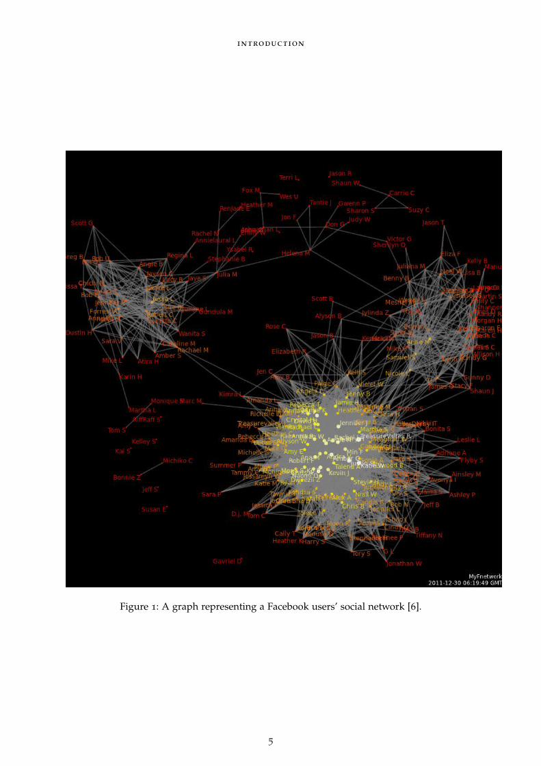
Graphs have a wide variety of real-world applications. In the area of social networks, graphsare composed of individuals and their relationships with others. Analysis of social networksled to the discovery of the small-world phenomena, which is also known as six degrees of sep-aration. The small-world property was first explored by Stanley Milgram in his small-worldexperiment [1]. His experiment consisted of sending letters randomly with instructions to for-ward the letter to a certain person. The letters were initially mailed to Omaha, Nebraska andWichita, Kansas, and the final recipients were in Boston. The letters instructed the randomrecipients to forward the letter back to its intended recipient in Boston. If the random recipi-ent did not know the final recipient’s address, they were instructed to forward it to someonethey thought would know the final recipient’s address. Many of the letters did not reachtheir intended targets, but of the ones that did, the average number of forwards required wasbetween 5 and 6. In one experiment, 160 letters were mailed out, of the 24 that were received,16 of them were correctly sent by a clothing merchant. The clothing merchant is an exampleof a hub in a social network, where one person is connected to many more than an averageperson.

With respect to biological networks, there are graphs that describe the interactions of pro-teins within cells. These graphs are referred to as protein-protein-interaction (PPI) networks.Comparing a diseased cellular network to a healthy one can provide insights for finding acure, and comparing the cellular networks of animals to those of their ancestors can helpexplain the evolutionary process.

In the area of electric power systems, graphs can be used to model the structure of a grid,and especially its resilience to blackouts. Through research in the field of power system pro-tection, we know that certain structures are more resilient to certain kinds of attacks. Ourcurrent power grid is less susceptible to random attacks, but the removal of key nodes canresult in large-scale disconnection and outages. The metrics to define those key nodes area substantial focus in related literature [2] [3] [4]. It should also be noted that, for exam-ple, a complete transient electromagnetic simulation of the US power grid is an extremelychallenging computational task, therefore using reduced models that can respond to variousparameters is a more feasible approach [5].

4

introduction

Figure 1: A graph representing a Facebook users’ social network [6].

5

2G R A P H S

A graph is commonly defined as a set of vertices and edges. Graphs are commonly referred toas networks, vertices are commonly referred to as nodes, and edges are commonly referred toas links or arcs. Generally the application of a graph dictates the terminology used to describeit. The degree of a vertex is the number of edges that are connected to it, or the number ofdirect neighbors it has. Directed graphs have a direction associated with each edge. In thispaper, we will focus on undirected graphs. A small undirected graph with numbered verticescan be seen below.

Figure 2: A small undirected graph with numbered vertices [7].

There are many different kinds of graphs (directed, undirected, regular, Hamiltonian) withmany different properties that define them. When comparing graphs, it is necessary to usestatistics in order to quantify differences and similarities between graphs. Some commonstatistics used to compare graphs are degree distribution, clustering coefficient, and networkdiameter.

The degree distribution of a graph counts the number of edges connected to each node,ranging from smallest degre to largest degree [8]. A degree distribution plot is a histogramwhere each bin contains the total number of nodes that have the number of edges indicatedby that bin. The degree distribution for our example graph can be seen in Figure 3.

The degree distribution is an important statistic because it can indicate whether or not agraph is scale-free. We will detail later the significance of scale-free graphs. A scale-free graphis a graph with many nodes that have a much higher degree than the average. Visually, thedifference between a scale-free graph and a non-scale-free graph is depicted in Figure 4.

Many real networks are best-modeled as scale-free networks [10] [11]. Social networks,power grids, journal papers, airline routes, etc. tend to have a few hubs with many connect-ing nodes [9]. However, power grids can differ significantly in some ways from scale-freenetworks [12]. The degree distribution of a scale-free network is power-law, which, mathe-matically, can be written as

P(k) ∼ k−a (1)

which gives the probability that a randomly-selected node has exactly k edges. For mostnetworks, the value of a is somewhere between two and three. A plot of a typical power-lawdistribution is seen below.

6

graphs

Figure 3: Degree distribution for our simple graph.

Figure 4: A random network (no hubs) and a scale-free network (three hubs). [9]

The clustering coefficient for a given node can be defined as the proportion of nodes thatare connected to it versus the greatest number of nodes that could be connected [14]. Theclustering coefficient for a given node can be computed by the fraction of possible trianglesthat exist within the graph. Mathematically, this is given as

cu =2T(u)

deg(u)(deg(u)− 1)(2)

where T(u) is the number of triangles through node u and deg(u) is the degree of u. Theclustering coefficient for node 1 of our example graph (Figure 2) is 1, because each of itsneighbors, 2 and 5, are connected. The clustering coefficient for node 4 is 0, because none of

7

graphs

Figure 5: An example power-law distribution. [13]

its neighbors, 3, 5, and 6, are connected. The global clustering coefficient is the mean of eachclustering coefficient of each node i,

Cglobal =1n

n

∑i=1

Ci (3)

The global clustering coefficient is a measure of how clustered a graph is overall. Forexample, the global clustering coefficient of a scale-free graph will be larger than that of atruly random graph.

Network diameter is defined as the longest path possible between any two nodes u and vin a network [15].

maxu,vd(u, v) (4)

Network diameter is related to the small-world property, which is the idea that any twonodes in a graph can be reached in a small number of steps. The concept of six degreesof separation, or that no two people are more than six friends apart, is an example of thesmall-world property.

These statistics can be easily used to show differences between networks, however graphsconstructed to have the same statistics could actually differ greatly in their behavior, as wehave seen in the power systems literature. This is a motivation to apply more advancedmetrics in order to understand the statistics of graphs that represent electric power networks.

8

2.1 graphlet degree distribution

2.1 graphlet degree distribution

In order to generalize the similarities and differences between power system graphs, we willuse a new metric that is introduced in the biological networks literature: the graphlet degreedistribution (GDD). The definition of GDD is similar to the regular degree distribution, asin fact GDD is a generalized version of the degree distribution [16]. The simple degreedistribution measures the number of edges touching each node. On the other hand, the GDDmeasures the number of subgraphs touching each node. A subgraph is defined here out of acomplete template graph composed by 5 nodes (can be larger). In this analysis we will use 29

graphlets, or orbits, as shown below.

Figure 6: The 29 graphlets used in our graphlet degree distribution comparison algorithm.[16]

In order to make a meaningful comparison between two graphs based on their degreedistribution, the measure of graphlet degree distribution agreement (GDD-A) is used. Thefollowing description is adapted from [16] .

For each orbit j, one needs to measure the j-th GDD,

djG(k) (5)

or the distribution of the number of nodes in G “touching” the corresponding graphlet at orbitj k times. The simple degree distribution, for example, is the 0th GDD, or the distribution forthe 2-node graphlet. (2) is scaled by k in order to decrease the contribution of larger degreesin a GDD.

SjG(k) =

djG(k)k

(6)

9

2.1 graphlet degree distribution

(3) is then normalized with respect to its total area,

T jG =

∞

∑k=1

SjG(k) (7)

giving

N jG(k) =

SjG(k)

T jG

(8)

The j-th GDD-agreement compares the j-th GDDs of two networks. For two networks Gand H and a particular orbit j, the “distance” D(G,H) between their normalized j-th GDDs is:

Dj(G, H) =1√2(

∞

∑k=1

[N jG(k)− N j

H(k)]2)

12 (9)

The distance is defined between 0 and 1, where 0 means that G and H have identical j-thGDDs, and 1 means that their j-th GDDs are far away. Next, D(G,H) is reversed to obtain thej-th GDD-agreement:

Aj(G, H) = 1− Dj(G, H), f orj ∈ {0, 1, . . . , 72} (10)

The total GDD-agreement between two networks G and H is the arithmetic or geometricaverage of the j-th GDD-agreements over all j

Aarith(G, H) =173

72

∑j=0

Aj(G, H) (11)

or

Ageo(G, H) =

(72

∏j=0

Aj(G, H)

) 173

(12)

GDD-agreement is scaled between 0 and 1, where 1 means that two networks are identicalin terms of GDD-A.

In order to determine the structure of our graphs, we will compare them to various randomnetwork models. The first one being used for comparison is the Erdos-Renyi (ER) model. Inthe ER model, the goal is to create a “truly” random graph with an average degree between2 and 3. An Erdos Renyi random network can be seen in Figure 4. A complete procedure forgenerating Erdos Renyi random graphs can be found in: [17]. We also compare the powersystem test case models with scale-free and minimum-distance graphs [18].

10

2.2 results

2.2 results

As a main power systems test dataset, we are using a model for the Polish grid. Using theGraphcrunch 2 software package, statistics such as degree distribution, average diameter, andclustering coefficient can be computed. Most importantly, we also obtain the pairwise GDD-Afor the Polish and synthetic graphs.

Figure 7: The Polish power grid model for Winter 1999.

Figure 7 is a rendering of the Polish power grid model that represents a snapshot for theWinter 1999-2000. The average degree is 2.422. The degree distribution is shown in Figure 8.

The degree distribution follows the exponential distribution seen in scale-free networks.[18]

We are also considering a different snapshot of the Polish power grid corresponding to Sum-mer 2004 during peak conditions. It is shown in Figure 9, along with its degree distributionin Figure 10.

Not surprisingly, its degree distribution is similar to that of the Winter 1999 graph showingthat the structure is fundamentally conserved over time in power grid networks.

We are also using a randomly generated graph based on the minimum-distance algorithm,which generates edges based on topological proximity to other nodes [18]. A new node ismore likely to connect to a nearby node rather than a far one. Graphs generated based onthis property exhibit a fat-tail property for their degree distribution as seen in Figures 11 and12, also consistent with empirical power grid models.

11

2.2 results

Figure 8: The degree distribution for the Winter 1999 Poland power grid model.

In addition to the Polish grid, we are also analyzing certain portions of the US grid. Anoverview of the division of Interconnections for the US (Eastern Interconnection, WesternInterconnection, Texas Interconnection) can be seen in Figure 13.

Finally, we present a table summarizing the key statistics for each graph:

Graph Average Degree NetworkDiame-ter

Average Clustering Coefficient

Poland Winter 1999 2.422 30 0.0122

Poland Summer 2004 2.555 30 0.015

Minimum-Distance 2.41 29 0.184

Eastern Interconnection 2.697 88 0.048

Texas Interconnection 2.592 34 0.024

Western Interconnection 2.695 68 0.065

12

2.3 gdd-a analysis

Figure 9: The Polish power grid model for Summer 2004.

2.3 gdd-a analysis

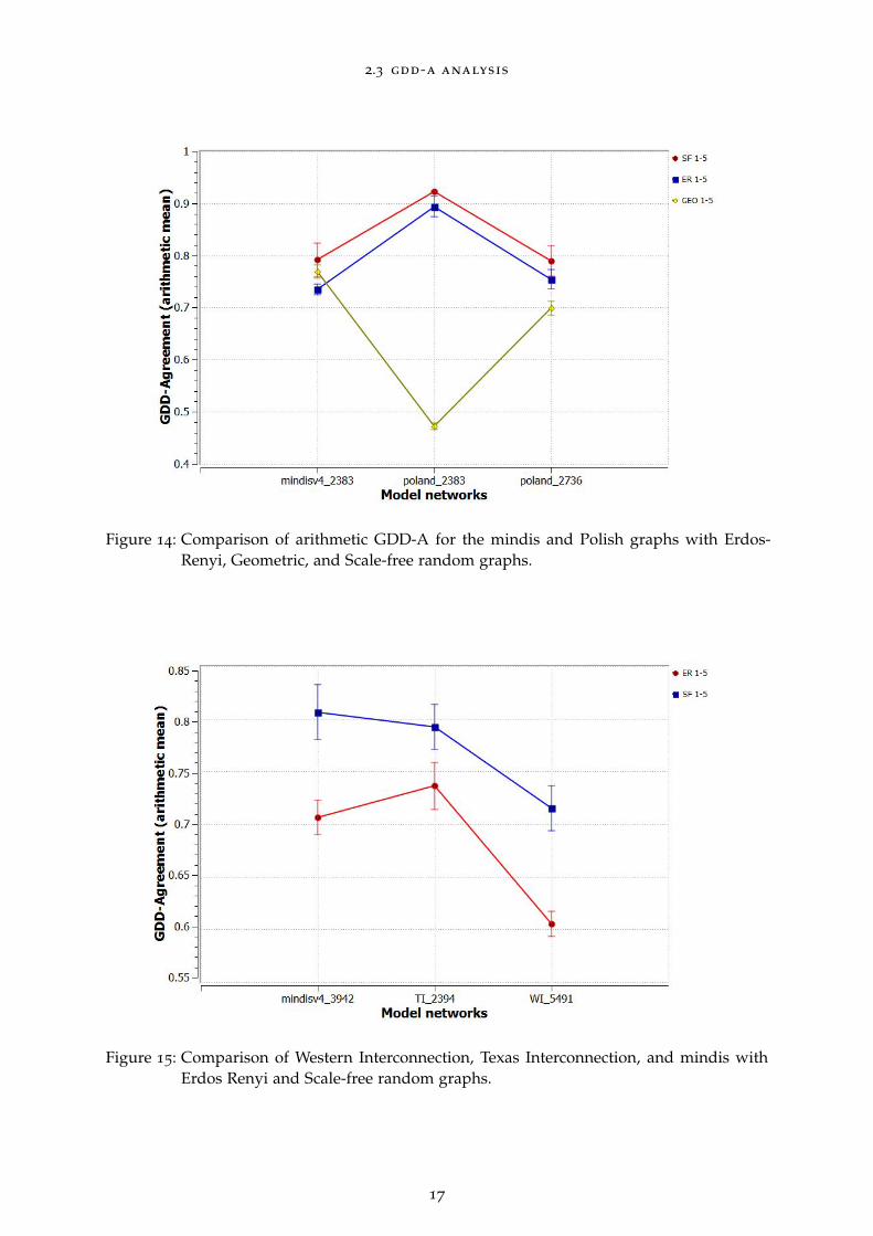
Figure 14 illustrates a comparison of the two Polish graphs and a minimum-distance graph tothe synthetized networks (random ER, geometric, and scale-free graphs). Scale free modelsconsistently agree with the power system models. Random ER also display high agreementwith the power system models. Geometric graphs show a high variation in the GDD-Acoefficients with respect to the Poland test case.

Figure 15 summarizes a similar analysis with respect to the US power networks (WesternInterconnection and Texas Interconnection) and a similarly sized minimum-distance graphwhere we kept the synthetic graphs with highest agreement (random ER, scale-free). Again,scale-free graphs show the maximum agreement with all US network subgrids. The randomER models show a similar pattern agreement but lower magnitudes for GDD-A.

As seen in figures 14 and 15, scale-free networks have the largest GDD-agreement with ourgraphs. The main characteristic of scale-free networks is the presence of hub nodes. Removalof hub nodes in a scale-free graph can result in disconnectivity between components of thegraph. Further removal of hub nodes would cause the remaining portions of the graph tomore closely resemble the Erdos Renyi random graph model.

13

2.3 gdd-a analysis

Figure 10: The degree distribution for the Summer 2004 Poland power grid model.

Of particular interest is also the dissimilarity seen between Polish winter test case and thegeometric random graph model. This is because in power grids node distance is determinedby electrical distance instead of physical distance. For example, two buses can be in closephysical proximity but have a large phase shift. For future reference, it would be better to usea model that accounts for both electrical distance and physical distance between nodes.

14

2.3 gdd-a analysis

Figure 11: A minimum-distance graph.

Figure 12: Degree distribution for the minimum-distance graph.

15

2.3 gdd-a analysis

Figure 13: US Power Grid Interconnections. [19]

16

2.3 gdd-a analysis

Figure 14: Comparison of arithmetic GDD-A for the mindis and Polish graphs with Erdos-Renyi, Geometric, and Scale-free random graphs.

Figure 15: Comparison of Western Interconnection, Texas Interconnection, and mindis withErdos Renyi and Scale-free random graphs.

17

3

C L U S T E R I N G

Clustering is an unsupervised machine learning algorithm used in many fields, such as imageprocessing, data analytics, and bioinformatics. In this chapter we use an electrical distancemetric [18] to cluster the buses from the Polish winter test case.

With respect to power grids, clustering of buses can help with power system protection.The electrical structure of a grid (voltage phase angle between generators) can be modeled asa graph, with each node having a certain phase angle. The nodes can then be grouped intoclusters based on similarity of voltage phase angle [20].

For our experiment, we are using the Poland Winter 1999 test case. As before, it consistsof 2383 buses and 6 zones. For our purposes, we can think of each zone as an “original”cluster according to the design of the system. A rendering of the Polish grid with the originalclusters based on zones can be seen in Figure 16.

Figure 16: Clustering of Polish Winter Test Case based on zones

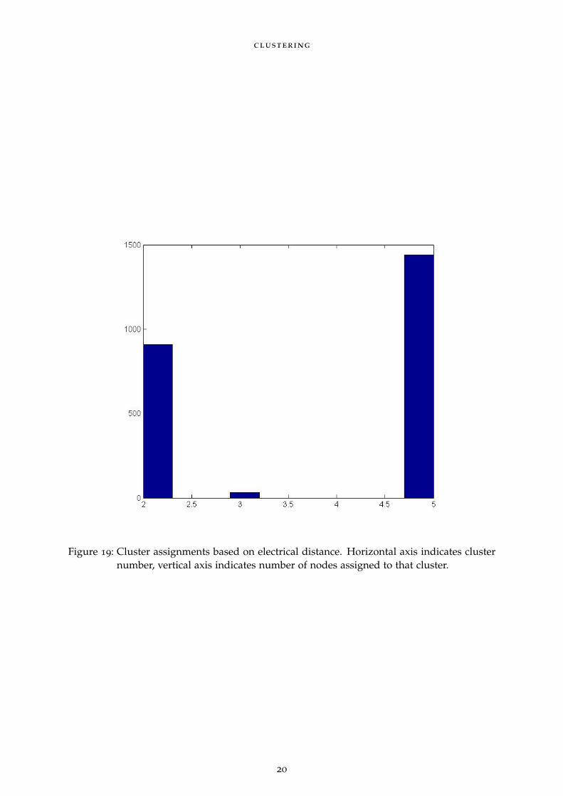
Instead of clustering based on physical space, we assigned clusters based on electricaldistance. The first step of procedure is to convert the Ybus for the power system into anelectrical distance matrix. Next, find the smallest average electrical distance between nodes.This resulted in only 3 clusters, instead of the original 6. This indicates that many nodes inthe grid are not distant from one another electrically speaking.

18

clustering

Figure 17: Clustering of Polish Winter Test Case based on electrical distance.

Figure 18: Orginal cluster assignments histogram. Horizontal axis indicates cluster number,vertical axis indicates number of nodes assigned to that cluster.

19

clustering

Figure 19: Cluster assignments based on electrical distance. Horizontal axis indicates clusternumber, vertical axis indicates number of nodes assigned to that cluster.

20

4

C O N C L U S I O N S

We compared synthetic graphs to real power networks according to a higher dimensionalmetric that measures the degree distribution with respect to a set of graphlets, the GraphletDegree Distribution Agreement. We find that scale-free networks agree with several empiricalpower system networks. Similarly, Erdos Renyi random graphs also suggest similarity interms of GDD-A. On the other hand, geometrical graphs did not consistently score high inthis regard.

We also test the cluster accuracy of the Polish grid for a metric of electrical distance. Wefound that clustering based on electrical distance reduces the number of clusters with respectto the original partition for this system (which was based on topological distance). Thisindicates that there are many nodes in the network that are close in an electrical sense.

21

B I B L I O G R A P H Y

[1] J. Travers and S. Milgram, “An experimental study of the small world problem,”Sociometry, vol. 32, no. 4, pp. 425–443, Dec. 1969. [Online]. Available: http://links.jstor.org/sici?sici=0038-0431%28196912%2932%3A4%3C425%3AAESOTS%3E2.0.CO%3B2-W

[2] E. Cotilla-Sanchez, P. Hines, C. Barrows, S. Blumsack, and M. Patel, “Multi-attributepartitioning of power networks based on electrical distance,” Power Systems, IEEE Trans-actions on, vol. 28, no. 4, pp. 4979–4987, Nov 2013.

[3] A. F. S.Arianos, E.Bompard, “Power grids vulnerability: a complex network approach,”Chaos, 2009.

[4] K. Atkins, J. Chen, V. S. A. Kumar, and A. Marathe, “The structure of electrical networks:a graph theory based analysis.” IJCIS, vol. 5, no. 3, pp. 265–284, 2009. [Online]. Available:http://dblp.uni-trier.de/db/journals/ijcritis/ijcritis5.html#AtkinsCKM09

[5] R. Albert, I. Albert, and G. L. Nakarado, “Structural vulnerability of the North Americanpower grid,” Physical Review E, vol. 69, 2004.

[6] [Online]. Available: http://commons.wikimedia.org/wiki/File:Kencf0618FacebookNetwork.jpg

[7] [Online]. Available: http://commons.wikimedia.org/wiki/File:6n-graf.svg

[8] R. Albert and A. laszlo Barabasi, “Statistical mechanics of complex networks,” Rev. Mod.Phys, p. 2002.

[9] C. Castillo, “Effective web crawling,” Ph.D. dissertation, University of Chile, 11 2004.

[10] A.-L. Barabasi and R. Albert, “Emergence of scaling in random networks,”Science, vol. 286, no. 5439, pp. 509–512, 1999. [Online]. Available: http://www.sciencemag.org/cgi/content/abstract/286/5439/509

[11] S. Boccaletti, V. Latora, Y. Moreno, M. Chavez, and D.-U. Hwang, “Complex networks :Structure and dynamics,” Phys. Rep., vol. 424, no. 4-5, pp. 175–308, Fervier 2006.

[12] P. Hines, S. Blumsack, E. Cotilla Sanchez, and C. Barrows, “The topological and electri-cal structure of power grids,” in System Sciences (HICSS), 2010 43rd Hawaii InternationalConference on, Jan 2010, pp. 1–10.

[13]

[14] D. Watts and S. Strogatz, “Collective dynamics of ‘small-world’ networks,” NATURE, vol.393, no. 6684, pp. 440–442, JUN 4 1998.

[15] E. W. Weisstein, “Graph diameter,” Internet, jan, weisstein, Eric W.

[16] N. Przulj, “Biological network comparison using graphlet degree distribution,”Bioinformatics, vol. 23, no. 2, pp. e177–e183, 2007. [Online]. Available: http://bioinformatics.oxfordjournals.org/content/23/2/e177.abstract

22

Bibliography

[17] P. Erdos and A. Renyi, “On random graphs. I,” Publ. Math. Debrecen, vol. 6, pp. 290–297,1959.

[18] E. Cotilla-Sanchez, “A complex network approach to analyzing the structure and dynam-ics of power grids,” 2009.

[19] [Online]. Available: http://commons.wikimedia.org/wiki/File:NERC-map-en.svg

[20] E. Hogan, E. Cotilla-Sanchez, M. Halappanavar, S. Wang, P. Mackey, P. Hines,and Z. Huang, “Towards effective clustering techniques for the analysis ofelectric power grids,” in Proceedings of the 3rd International Workshop on HighPerformance Computing, Networking and Analytics for the Power Grid, ser. HiPCNA-PG ’13. New York, NY, USA: ACM, 2013, pp. 1:1–1:8. [Online]. Available:http://doi.acm.org/10.1145/2536780.2536785

23