Power and Bandwidth allocationfor High-Throughput Satellites

using Particle Swarm Optimization

Author:

Nils Pachler de la Osa

Supervisors:

Prof. Edward Crawley

Dr. Bruce Cameron

Engineering Systems LaboratoryDepartment of Aeronautics and Astronautics

Massachusetts Institute of Technology10/02/2019

Abstract

In the recent years, communications satellites have been evolving from static payloads to highly flex-ible components. Modern satellites are able to provide four orders of magnitude higher throughputthan their ancestors fourty years ago, going from the few Mbps with the first commercial communi-cation satellite to the hundreds of Gbps of current approaches. This enhancement in performanceaims to cover an ever-increasing highly variable demand. An automatic tool able to dynamicallymanage the satellites’ resources, despite optional in the early years of this industry, has become anecessity.

Academic interest in the resource allocation problem for satellite communications has beengrowing in the last years. Previous literature show successful implementations of a vast varietyof algorithms (mathematical programming, heuristic and metaheuristic approaches, etc) for theseparate power and bandwidth allocation problems. Some research has also been focused on thejoint problem, but the number of implementations is low. Moreover, the number of successfulimplementations is furtherly reduced when considering time restrictions. This thesis aims to providea new implementation of a metaheuristic, commonly known to be fast, to solve the joint power andbandwidth allocation in a real case scenario, where the time restrictions are a constraint.

To do so, the satellite communications context in first introduced. Then, the joint problem,including the variables, restrictions and metrics, is formulated and the simulation model is ex-plained. At this point, the Particle Swarm Optimization implementation is provided and each ofthe functionalities of the algorithm is explained and detailed.

The results show a fast convergence of the implementation, reaching a good enough solutionin under 10s, but getting stuck in a local optima. To solve this problem, a hybrid version of thealgorithm combined with a genetic algorithm is developed. The new results show that the hybridis a well suited implementation for the power allocation problem, as it consistently improves theGA-only results. For the joint problem, it provides an 80% power reduction and 2% lower unmetdemand than the GA-only in the low runtime scenario.

i

Resum

En els ultims anys, els satel·lits de comunicacions han evolucionat des d’una carrega util estaticafins a components completament dinamics. Els satel·lits moderns son capacos de proveir quatreordres de magnitud mes data rate que els seus predecessors quaranta anys abans, anant des delspocs Mbps amb el primer satel·lit de comunicacions comercial fins als centenars de Gbps delsdarrers plantejaments. Aquest increment en rendiment intenta cobrir una sempre creixent i canviantdemanda. Una eina automatica capac de gestionar dinamicament els recursos dels satel·lits, tot ique opcional en els primers anys d’aquesta industria, es ara una necessitat.

L’interes academic en el problema d’assignacio de recursos en un satel·lit ha crescut els ultimsanys. Literatura previa mostra implementacions exitoses d’una gran varietat d’algoritmes (progra-macio matematica, plantejaments heurıstics i metaheurıstics, etc) pels problemes d’assignacio depotencia i d’ample de banda. Alguns treballs tambe s’han centrat en el problema conjunt, pero elnombre d’implementacions es baix. A mes a mes, el nombre d’implementacions exitoses es encarames reduıt quan es consideren restriccions temporals. Aquesta tesis te com a objectiu proporcionaruna nova implementacio d’una metaheurıstica, coneguda per la seva rapida convergencia, per solu-cionar el problema conjunt d’assignacio de potencia i ample de banda en un escenari real, on lesrestriccions temporals estan a l’ordre del dia.

Amb aquest objectiu, primer s’introdueix el context de comunicacions de satel·lits. Seguidament,es formula el problema conjunt, incloent les variables, restriccions i metriques, i s’explica el modelde simulacio. En aquest moment, es proveeix la implementacio del Particle Swarm Optimization is’expliquen i detallen cada una de les funcionalitats de l’algoritme.

Els resultats mostren una rapida convergencia de la implementacio, aconseguint una suficient-ment bona solucio en menys de 10s, pero convergint a un optim local. Per solucionar aquestproblema, es desenvolupa una versio hıbrida de l’algoritme, combinant-lo amb un Genetic Algo-rithm. Els nous resultats mostren que l’hıbrid es un algoritme adequat per resoldre el problema del’assignacio de potencia, ja que, de manera consistent, millora els resultats de la implementacio delGA. Pel problema conjunt, proporciona un 80% de reduccio de potencia i un 2% de reduccio endemanda no satisfeta en escenaris de baix temps d’execucio.

ii

Resumen

En los ultimos anos, los satelites de comunicaciones han evolucionado desde una carga util estaticahasta componentes enteramente dinamicos. Los satelites modernos son capaces de proveer cuatroordenes de magnitud mas data rate que sus predecesores cuarenta anos antes, pasando de los pocosMbps con el primer satelite de comunicaciones comercial hasta los centenares de Gbps de los ultimosplanteamientos. Este incremento en rendimiento intenta cubrir una siempre creciente y cambiantedemanda. Una herramienta capaz de gestionar dinamicamente los recursos de los satelites, aunqueopcional en los primeros anos de esta industria, es ahora una necesidad.

En interes academico en el problema de asignacion de recursos en un satelite ha crecido enlos ultimos anos. Literatura previa muestra implementaciones exitosas de una gran variedad dealgoritmos (programacion matematica, planteamientos heurısticos y metaheurısticos, etc) para losproblemas de asignacion de potencia y ancho de banda. Algunos trabajos tambien se han centradoen el problema conjunto, pero el numero de implementaciones es bajo. Ademas, el nombre deimplementaciones exitosas es aun mas reducido cuando se consideran restricciones temporales. Estatesis tiene como objetivo proporcionar una nueva implementacion de una metaheurıstica, conocidapor su rapida convergencia, para solucionar el problema conjunto de asignacion de potencia i anchode banda en un escenario real, donde las restricciones temporales estan a la orden del dia.

Con este objetivo, primero se introduce el contexto de comunicaciones de satelites. Seguida-mente, se formula el problema conjunto, incluyendo las variables, restricciones y metricas, y seexplica el modelo de simulacion. En este momento, se provee la implementacion del Particle SwarmOptimization y se explican y detallan cada una de las funcionalidades del algoritmo.

Los resultados muestran una rapida convergencia de la implementacion, consiguiendo una sufi-cientemente buena solucion en menos de 10s, pero convergiendo a un mınimo local. Para solucionareste problema, se desarrolla una version hıbrida del algoritmo, combinandolo con un Genetic Al-gorithm. Los nuevos resultados muestran que el hıbrido es un algoritmo adecuado para resolverel problema de asignacion de potencia, ya que, de manera consistente, mejora los resultados de laimplementacion del GA. Para el problema conjunto, proporciona un 80% de reduccion en potenciay un 2% de reduccion en demanda no satisfecha en escenarios de bajo tiempo de ejecucion.

iii

Acknowledgements

First, I would like to thank Prof. Edward Crawley and Dr. Bruce Cameron for their unconditionalsupport during my stay at MIT. Together, they introduced me to System Architecture and showedme new ways of facing a problem. Ed, Bruce, thank you for all the advice I have received regardingpersonal and professional endeavours. Truly, it has been an honor to work with you.

Special thanks to Juan Jose Garau for all the advice and counseling since my arrival at MITearlier this year. Juanjo, thank you for sharing your experience and skills with me, both in academicand personal environments. I would also like to thank Markus Guerster, for the development of thesimulation model used in this thesis, and Inigo del Portillo, for his research and programming tips.

I don’t want to miss the chance to thank Prof. Alejandro Pajuelo, professor at UPC, and Prof.Miguel Angel Barja, director of CFIS, without whom this project would not have been possible.Thank you for fulfilling my dream of studying at MIT. There are many other individuals aroundthe campus that helped to make my time at MIT unique. It would be too lengthy to list them all.

I would like to thank SES S.A. and the Fundacio Cellex for the financial support during thedevelopment of this thesis and my stay in Boston.

Finally, but not less important, I would like to thank my parents, Jørn and Nina, for theirunconditional support and love during my whole life. Thank you both for all you gave me and theknowledge and skills that have helped me achieve my dreams.

iv

Contents

1 Introduction 1

1.1 Motivation . . . . . . . . . . . . . . . . . . . . . . . . . . . . . . . . . . . . . . . . . 1

1.2 General objectives . . . . . . . . . . . . . . . . . . . . . . . . . . . . . . . . . . . . . 2

1.3 Background . . . . . . . . . . . . . . . . . . . . . . . . . . . . . . . . . . . . . . . . . 2

1.4 Specific objective . . . . . . . . . . . . . . . . . . . . . . . . . . . . . . . . . . . . . . 3

1.5 Overview . . . . . . . . . . . . . . . . . . . . . . . . . . . . . . . . . . . . . . . . . . 3

2 Satellite Communications System 4

2.1 Information theory applied to space communications . . . . . . . . . . . . . . . . . . 5

2.1.1 Channel: electromagnetic sub-space . . . . . . . . . . . . . . . . . . . . . . . 5

2.1.2 Antennas . . . . . . . . . . . . . . . . . . . . . . . . . . . . . . . . . . . . . . 6

2.2 Link budget equation: calculating the receiving power . . . . . . . . . . . . . . . . . 9

2.2.1 Electromagnetic disturbances . . . . . . . . . . . . . . . . . . . . . . . . . . . 10

2.2.2 Signal to noise ratio . . . . . . . . . . . . . . . . . . . . . . . . . . . . . . . . 13

2.3 Data Rate . . . . . . . . . . . . . . . . . . . . . . . . . . . . . . . . . . . . . . . . . . 13

3 Model description 15

3.1 Problem formulation . . . . . . . . . . . . . . . . . . . . . . . . . . . . . . . . . . . . 15

3.1.1 Problem’s variables . . . . . . . . . . . . . . . . . . . . . . . . . . . . . . . . . 15

v

3.1.2 Restrictions . . . . . . . . . . . . . . . . . . . . . . . . . . . . . . . . . . . . . 17

3.1.3 Metrics: Unmet Demand and Power . . . . . . . . . . . . . . . . . . . . . . . 17

3.2 Simulation model . . . . . . . . . . . . . . . . . . . . . . . . . . . . . . . . . . . . . . 18

3.2.1 User terminal . . . . . . . . . . . . . . . . . . . . . . . . . . . . . . . . . . . . 18

3.2.2 Carrier . . . . . . . . . . . . . . . . . . . . . . . . . . . . . . . . . . . . . . . 19

3.2.3 Beam . . . . . . . . . . . . . . . . . . . . . . . . . . . . . . . . . . . . . . . . 19

3.2.4 Satellite . . . . . . . . . . . . . . . . . . . . . . . . . . . . . . . . . . . . . . . 19

3.2.5 Constellation . . . . . . . . . . . . . . . . . . . . . . . . . . . . . . . . . . . . 20

4 Metaheuristics approach 21

4.1 Particle Swarm Optimization: PSO . . . . . . . . . . . . . . . . . . . . . . . . . . . . 21

4.1.1 Flight . . . . . . . . . . . . . . . . . . . . . . . . . . . . . . . . . . . . . . . . 22

4.1.2 Global and local bests . . . . . . . . . . . . . . . . . . . . . . . . . . . . . . . 23

4.1.3 Implementation . . . . . . . . . . . . . . . . . . . . . . . . . . . . . . . . . . . 24

4.1.4 Heuristics . . . . . . . . . . . . . . . . . . . . . . . . . . . . . . . . . . . . . . 26

4.1.5 Parameter selection . . . . . . . . . . . . . . . . . . . . . . . . . . . . . . . . 27

4.2 Genetic Algorithm: GA . . . . . . . . . . . . . . . . . . . . . . . . . . . . . . . . . . 27

5 Results 29

5.1 Traffic model . . . . . . . . . . . . . . . . . . . . . . . . . . . . . . . . . . . . . . . . 29

5.2 Simulation parameters . . . . . . . . . . . . . . . . . . . . . . . . . . . . . . . . . . . 30

5.3 Scenario 1: Power allocation . . . . . . . . . . . . . . . . . . . . . . . . . . . . . . . . 30

5.3.1 Sub-scenario 1: Low demand . . . . . . . . . . . . . . . . . . . . . . . . . . . 30

5.3.2 Sub-scenario 2: Balanced demand . . . . . . . . . . . . . . . . . . . . . . . . 32

5.3.3 Sub-scenario 3: Excess demand . . . . . . . . . . . . . . . . . . . . . . . . . . 33

5.4 Scenario 2: Optimizing power and bandwidth . . . . . . . . . . . . . . . . . . . . . . 34

vi

5.4.1 Sub-scenario 1: Low demand . . . . . . . . . . . . . . . . . . . . . . . . . . . 34

5.4.2 Sub-scenario 2: Balanced demand . . . . . . . . . . . . . . . . . . . . . . . . 35

5.4.3 Sub-scenario 3: Excess demand . . . . . . . . . . . . . . . . . . . . . . . . . . 36

6 Conclusions 38

6.1 Conclusions and remarks . . . . . . . . . . . . . . . . . . . . . . . . . . . . . . . . . . 38

6.2 Future work . . . . . . . . . . . . . . . . . . . . . . . . . . . . . . . . . . . . . . . . . 39

Appendices 40

A PSO-GA: a hybrid approach 41

A.1 Implementation of a PSO-GA . . . . . . . . . . . . . . . . . . . . . . . . . . . . . . . 41

A.2 PSOGA+ . . . . . . . . . . . . . . . . . . . . . . . . . . . . . . . . . . . . . . . . . . 42

A.3 Simulation parameters . . . . . . . . . . . . . . . . . . . . . . . . . . . . . . . . . . . 42

B Scenario 2 complete results 44

vii

List of Figures

2.1 Information Theory Diagram . . . . . . . . . . . . . . . . . . . . . . . . . . . . . . . 4

2.2 Information Theory applied to Space Communications (EM: Electromagnetic) . . . . 5

2.3 Division of frequency spectrum [1] . . . . . . . . . . . . . . . . . . . . . . . . . . . . 6

2.4 Example of a linear polarization [2] . . . . . . . . . . . . . . . . . . . . . . . . . . . . 7

2.5 Gain of a parabolic antenna [3] . . . . . . . . . . . . . . . . . . . . . . . . . . . . . . 8

3.1 Prefixed division of the frequency pool into beams (shades) and variable division ofthe prefixed slots into 3 carriers (C, dashed lines) . . . . . . . . . . . . . . . . . . . . 16

3.2 Graphical representation of resource’s variables . . . . . . . . . . . . . . . . . . . . . 17

3.3 Class diagram for the simulated model . . . . . . . . . . . . . . . . . . . . . . . . . . 18

4.1 Particle’s position and initialization . . . . . . . . . . . . . . . . . . . . . . . . . . . . 25

5.1 Scenario 1, Pareto Front for Low demand . . . . . . . . . . . . . . . . . . . . . . . . 31

5.2 Scenario 1, Pareto Front for Low demand, including the hybrid . . . . . . . . . . . . 31

5.3 Scenario 1, Pareto Front for Balanced demand . . . . . . . . . . . . . . . . . . . . . 32

5.4 Scenario 1, Pareto Front for Balanced demand, including the PSOGA+ . . . . . . . 33

5.5 Scenario 1, Pareto Front for Excess demand . . . . . . . . . . . . . . . . . . . . . . . 33

5.6 Scenario 2, 18h timestamp, Pareto Front for Low demand . . . . . . . . . . . . . . . 35

5.7 Scenario 2, 0h timestamp, Pareto Front for Balanced demand . . . . . . . . . . . . . 35

5.8 Scenario 2, 9h timestamp, Pareto Front for Excess demand . . . . . . . . . . . . . . 36

viii

A.1 Particle swarm optimization convergence in 18 iterations . . . . . . . . . . . . . . . . 42

B.1 Scenario 2, 0h timestamp, Pareto Front for Low demand . . . . . . . . . . . . . . . . 45

B.2 Scenario 2, 9h timestamp, Pareto Front for Low demand . . . . . . . . . . . . . . . . 46

B.3 Scenario 2, 18h timestamp, Pareto Front for Low demand . . . . . . . . . . . . . . . 47

B.4 Scenario 2, 0h timestamp, Pareto Front for Balanced demand . . . . . . . . . . . . . 48

B.5 Scenario 2, 9h timestamp, Pareto Front for Balanced demand . . . . . . . . . . . . . 49

B.6 Scenario 2, 18h timestamp, Pareto Front for Balanced demand . . . . . . . . . . . . 50

B.7 Scenario 2, 0h timestamp, Pareto Front for Excess demand . . . . . . . . . . . . . . 51

B.8 Scenario 2, 9h timestamp, Pareto Front for Excess demand . . . . . . . . . . . . . . 52

B.9 Scenario 2, 18h timestamp, Pareto Front for Excess demand . . . . . . . . . . . . . . 53

ix

List of Tables

5.1 PSO and GA parameter selection . . . . . . . . . . . . . . . . . . . . . . . . . . . . . 30

A.1 PSOGA and PSOGA+ parameter selection . . . . . . . . . . . . . . . . . . . . . . . 43

x

Nomenclature

Acronyms

GA Genetic Algorithm

ITU International TelecommunicationUnion

MD Met Demand

MODCOD Modulation and Coding

PSO Particle Swarm Optimization

SINR Signal to Interference plus NoiseRatio

UD Unmet Demand

Common sub-indices

3dB Value in the 3dB threshold

R Receiving antenna

T Transmitting antenna

u User

Symbols

Γ Spectral efficiency

λ Wavelength

θ Angle with reference to the beampointing

A Area

c Speed of light

D Antenna diameter

f Frequency

G Gain

k Boltzmann constant

N Noise power

P Power

R Data rate

r Antenna radius

T Temperature

W Watt

xi

Chapter 1

Introduction

1.1 Motivation

Since its beginnings in the early 60s, the satellite communications market has experienced anexponential growth which does not seem to stop any time soon. While in the early years of thisindustry a communications satellite was only able to manage a few phone lines (few Mbps), a rapidevolution of on-board technology and an increase in power generation led to the development ofthe so-called High-Throughput Satellites (HTS), able to provide tens and even hundreds of Gbps.According to recent reports [4][5], the growth in demand is expected to continue over the next years.

The growth in the first decades of the industry was heavily boosted by an increase the launcher’scapacity, allowing higher power generation, which is directly related with the satellite’s capacity.This factor, however, eclipsed the impact of the payload’s technology evolution. In the last decades,however, the launcher’s capacity growth has seemed to stall while the development of on-boardpayload has become crucial to maintain the growth imposed by the demand.

Within early stages of this industry, those resources where assigned once, prior to the launchof the satellite, directly depending on the contract signed with the users. This works perfectlywhen the users consume exactly the amount of data rate demanded at every time. However, theharsh reality is that the data consumed is bursty. The nature of current systems is based on highlyfluctuating consumption, as it depends on single individuals’ behaviour. The static assignation ofresources incurs in a waste of power and bandwidth when the demand is not maximal, which happensfrequently. To solve this problem, satellite manufacturers have developed highly flexible payloadsable to change the assignation of resources much more often than once in a lifetime. Thanks torecent technology improvements, satellite’s payload have evolved from static preassigned resourcesto fully dynamic components, able to change their behaviour based on on-ground command. Asan example, current satellite operators are planning to launch new constellations able to managethousands of fully re-configurable beams (multi-beam architectures), while able to change frequencyand power on command.

1

While this allows for a better satisfaction of the demand, both in terms of quality of service andrevenues, it comes at the expense of a higher complexity in the dynamic management. Althoughmanual resource allocation was well suited for static management, it is unfeasible for the newgeneration of satellite communications. An automatic tool has to be developed to fully exploit thenovel capabilities. The problem underlying the development of this tool is known as the resourceallocation (RA) problem.

1.2 General objectives

The main purpose of this thesis is to solve the allocation of power and bandwidth within the RAproblem for High-throughput multibeam Satellites. To this end, this thesis proposes the applicationof a new algorithm to solve the joint problem. Finally, this work compares and tests the newimplementation against a predefined baseline.

1.3 Background

The Resource Allocation (RA) problem in the context of satellite communications has been pro-foundly studied in the recent years. Within the RA problem, literature often identifies four resourcesto allocate: radio-transmitted power, radio-transmission frequency, beam pointing and beam shape.For this thesis, the literature review is divided in three parts: power allocation, frequency assign-ment and the joint problem. The following paragraphs comprise the work for each of these fields.

The power allocation problem consists of assigning the power level for each transmitting beamwithin a satellite. The problem is known to be NP-hard and hard to approximate when the satel-lite’s power generation is not enough to satisfy the power demand [6]. In the recent years, manyapproaches have been developed to solve this problem. Authors in [7] propose a convex optimizationtechnique to find the trade-off between system capacity and the fairness between users. Work [8]tries to find a solution with a heuristic based on Lagrange multipliers. Regarding more modern tech-niques, [6] uses a hybrid between the Simmulated Annealing and Genetic Algorithm metaheuristicsto solve a multiobjective formulation of the problem, while [9] uses a Particle Swarm OptimizationApproach to solve a single objective formulation. The authors in [10] rely on a Deep ReinforcementLearning technique to find a solution. All these studies try to distribute the available power poolinto different carriers and beams to meet users’ demand.

The frequency assignment problem consists of dividing the frequency pool, either in the fre-quency domain (beam coloring) or in the time domain (beam hopping), among beams to fulfil thedemand of each user. As the power allocation problem, the frequency assignment is known to beNP hard and hard to approximate [11]. Starting with mathematical programming, this problemhas also been solved using heuristic approaches [12] and convex optimization [13]. Regarding ar-tificial intelligence and machine learning approaches, [14] proposes a deep reinforcement learningmethodology, while [15] uses a hybrid neural network combined with a Genetic Algorithm.

2

Both problems have also been studied together in recent literature. Authors in [16] propose analgorithm to minimize co-channel interference. This problem has also been studied in [17] followinga Genetic Algorithm approach. Both works show significant improvements in power when allocatingjoint power and bandwidth compared to only power allocation. None of this works, however, teststhe algorithms under time restriction conditions, crucial for real applications.

1.4 Specific objective

The specific purpose of this thesis is to solve the joint power and bandwidth allocation problemfor multibeam HTS by formulating the problem as a multi-objective problem and solving it usingParticle Swarm Optimization (PSO). To this purpose, this thesis presents this new implementationof the algorithm for the joint problem, while benchmarking the algorithm for several test cases ina realistic environment.

1.5 Overview

The following lines give a general overview of this thesis and its main sections.

Chapter 2 gives a brief introduction of the Satellite Communication context. The main elementsthat interact in a communication are explained in section 2.1. The equations that govern the systemare presented in section 2.2. Finally, the the metric used in this work for satellite communicationssystems is introduced in 2.3.

Chapter 3 describes the model used to formulate and solve the problem. The formulation,metrics and variables used are presented in section 3.1. A short grasp to the simulation model isgiven in section 3.2.

Chapter 4 gives a detailed explanation of the metaheuristic used to solve the problem, as well asa secondary metaheuristic used to compare the solution space. The Particle Swarm Optimizationalgorithm and its implementation is discussed in section 4.1. An overview of the Genetic Algorithmis given in section 4.2.

Chapter 5 presents and discusses the results of this thesis. Refer to sections 5.3 and 5.4 for thethree studied scenarios.

Chapter 6 concludes with the main findings of this thesis and its implications in future work.

3

Chapter 2

Satellite Communications System

Information theory, presented in [18] over 50 years ago, mathematically describes the entities andrelations in a general communication system. As a general overview, it exposes 6 elements thattake part in the information’s flow:

• Information Source: starting point of the communication.

• Transmitter : element in charge of emitting the message.

• Transmitting Medium: physical link between transmitter and receiver.

• Receiver : element in charge of receiving the message.

• Destination: end point of the communication.

• Noise Source: interference in the message due to disturbances in the Transmitting Medium.

The flow of this system is clear and is the source of the known diagram shown in figure 2.1.

Information

SourceTransmitter

Transmitting

MediumReceiver Destination

Noise Source

Message

Signal

Transmitted Received

Signal

Message

Figure 2.1: Information Theory Diagram

Space communications accurately follow the description presented in [18]. In the following lines,an introduction and brief explanation of all the elements will be given while the laws and equationsthat govern the system will be presented and explained. 1

1This thesis briefly resumes the information presented in [3]. Refer to this source for further clarification.

4

2.1 Information theory applied to space communications

Space communications are vastly governed by two interlocutors: ground stations and satellites.Ground stations are entities located in the surface of the Earth that demand a flow of commu-nication. Satellites, on the other hand, are entities located in orbits around the Earth in chargeof satisfying this demand. These two entities are associated with the endpoints of the communi-cation (source and destination). The exact mapping depends on the direction of the information.Standardization defines the following directions:

• Uplink : from ground stations (source) to satellites (destination).

• Downlink : from satellites (source) to ground stations (destination).

• Intersatellite links: between satellites.

In order to get the information from the source to the destination, space communications rely onantennas. Antennas are devices able to convert electric signals into electromagnetic waves andvice-versa. Each endpoint, then, requires an antenna to establish the communication. Followingthis definition, antennas fulfil the roles of transmitting and receiving entities, as their main functionis to interact the endpoints with the medium.

From the description of antennas, it can be seen that the Transmitting Medium is the electromag-netic space between the two antennas. The noise, then, are the disturbances in this electromagneticspace.

With all the elements described, the mapping of figure 2.1 to space communications can bedirectly done:

Ground St.

Satellite

Transmitting

AntennaEM Noise

Receiving

Antenna

Satellite

Ground St.

EM

disturbances

Message Transmitted

Signal

Received

Signal

Message

Figure 2.2: Information Theory applied to Space Communications (EM: Electromagnetic)

2.1.1 Channel: electromagnetic sub-space

The electromagnetic waves are responsible of transmitting the information from the transmitter tothe receiver. These waves are primarily defined by three factors:

• Power : determines the wave’s travel distance. This parameter is crucial for satellite commu-nications as it restricts the wave’s reachable destinations.

5

• Frequency : Rate of oscillation of the signal. Due to the limitation in the accessible frequencies,an international organization (International Telecommunication Union, ITU) is responsible ofdividing the frequency space into the different sectors that use it. For space communications,the ITU has assigned different bands (figure 2.3), which are further subdivided into channels.This thesis assumes the utilization of the Ka band (26.5 - 40GHz) for the communications.Channels are arbitrarily defined sub-bands of the frequency space that have an ideal maximumthroughput related to the bandwidth associated. Therefore, the system’s capacity is directlyrelated with the number of channels in use and the bandwidth of each channel.

Figure 2.3: Division of frequency spectrum [1]

• Polarization: Any electromagnetic wave is composed by an electric field component and amagnetic field component. These two components are orthogonal and perpendicular to thepropagation of the wave. The direction of these fields is arbitrary, defined by the emittingantenna. Any antenna that transmits or receives in a particular direction cannot transmitor receive in the opposite one. This permits doubling the effective bandwidth of the commu-nication, as two opposite polarizations can be transmitted without any interference betweenthem. Figure 2.4 shows a single wave polarization. Neither the electric, nor the magnetic fieldinterfere when the fields are orthogonal.

2.1.2 Antennas

An antenna is a device that converts an electrical signal into an electromagnetic wave and viceversa. Antennas are defined by two main parameters: gain and beamwidth, which determine theexact behaviour of the wave transmitted.

6

Figure 2.4: Example of a linear polarization [2]

Gain

Ratio of power transmitted or received per unit of solid angle with respect to the power transmittedor received per unit of solid angle by an isotropic antenna. Common antennas focus their powerinto a single or a subset of directions, which amplifies the power in those directions and reducesit in the others. Depending of the characteristics of the gain, different sub types of antennas aredefined:

• Isotropic: power in all directions is the same.

• Torus: increased power in a plane.

• Parabolic: increased power in a single direction.

The parabolic antenna is the most used in space communications, as the power requirementsare very restrictive and the position of the receiving antenna is known. The gain, thus, depends onthe direction considered and is maximized in the electromagnetic axis of the antenna (boresight).For parabolic antennas, the maximum gain is obtained by:

Gmax =4π

λ2Aeff (2.1)

Where λ is the wavelength and Aeff is the effective area of the antenna. The latter parameter

can be computed using the area of the antenna (A = πD2

4 ) and an efficiency parameter based onthe imperfections of the antenna (shape, obstacles, etc).

7

Beamwidth

The beamwidth defines the pattern of the gain in the different directions. In the parabolic antenna,the gain is focused in a single direction, but some directions still have residual gain:

Figure 2.5: Gain of a parabolic antenna [3]

As can be seen in 2.5, the gain is lobe-shaped and rapidly decays after the 3dB limit. That is,when computing the gain in dB (G(dB) = 10log(G)), the gain loss rapidly increases when surpassingthe limit G = Gmax − 3dB. Therefore, the range of the antenna lies within this margin (whichproduces a circular shape). This is called the beamwidth. Current technology allows multiplebeams per antenna, each with its own pointing and beamwidth. Also, modern approaches permitother shapes in the beam, but its technology and applications are outside the range of this thesis.

The angle of 3dB can be computed as

θ3dB = 70λ

D[rad] (2.2)

The gain with respect to θ3dB can be adjusted to the formula:

G(θ) = Gmax − 12

(θ

θ3dB

)2

[dB] (2.3)

For sufficiently small angles (0 < θ < θ3dB2 )

Antenna sub-systems

Although antennas have a fundamental role in space communications, they require from otherdevices to properly work. Within those, the following are usually found:

8

• Modulators: electronic systems capable of codifying a signal into an electronic wave, using aspecific MODCOD.

• Demodulators: inverse of modulators. These systems can be found in receiver antennas, whichmust first decode the wave to obtain the signal.

• Power amplifiers: electric systems capable of amplifying the power of an electromagneticwave.

• Signal processors: electronic systems in charge of the signal processing needed to perform thecommunication.

2.2 Link budget equation: calculating the receiving power

One of the most important factors in the design of a space communication system is the powerthat will be fed to the transmitting antenna. This value directly influences the power received atthe receiving antenna, which must be higher that the surrounding power level in order to correctlyidentify the signal.

With the defined gain parameter, the power transmitted is straight-forward to compute:

GTPT [W ] (2.4)

Where PT is the power radiated by an isotropic antenna, which is directly the power that feedsthe antenna. As the gain depends on the direction, is useful to characterize the power per unit ofsolid angle:

GTPT4π

[W

steradian

](2.5)

A receiver antenna with area A located at a distance r would be defined by a solid angle equalto:

A

r2[steradian] (2.6)

Thus, the received power in the destination antenna would be equal to:

PR =GTPT

4π

ARr2

[W ] (2.7)

Where GT can be assumed to be constant for AR

r2 << 1.

The receiver antenna is also defined by its gain and efficiency. Therefore:

9

PR =GTPT

4π

1

r2GR4πλ2

[W ] (2.8)

At this point, we can define the free space loss as LFS =(4πrλ

)2. The receiving power is then:

PR =GTGRLFS

PT [W ] (2.9)

This is known as the link budget equation. Usually, this formula is written in logarithmic form:

PR = PT +GT +GR − L (2.10)

Where X(dB) = 10log(X)

Due to the imperfections in the chain, the free space loss is not the only loss of the system.Electrical, thermal and other losses also degrade the quality of the link. It is notable that in thisequation all the losses have been unified in a single term L. In section 2.2.1, an explanation for allthe losses, except for the already explained LFS , can be found.

2.2.1 Electromagnetic disturbances

In order to be functional, receiving antennas have to be able to identify the signal from the receivedwave. To do so, the power of the wave has to be higher than the power of the surrounding noise.Thus, the ratio of signal power versus the noise power is a valuable metric to assess the correctidentification of the signal. This leads to the necessity of the noise characterization.

Noise is commonly defined as random interferences within a signal. This is translated to achange in the frequencies observed by the receiver. Thus, the noise can be defined by:

N = N0B[W ] (2.11)

Where N is the noise power, N0 the white noise power (random signal with equal intensity inall frequencies), and B the bandwidth of the signal.

In order to assimilate random noise with a physical meaning, the term noise temperature isused. Noise temperature is defined as:

T =N0

k(2.12)

Where k is the Boltzmann constant. This temperature T is the temperature at which a resistorproduces the noise N0.

Characterizing the noise for a single element simply becomes knowing its analog noise tem-perature. Modern systems, however, rely on a succession of elements to work and therefore it is

10

necessary to characterize the noise in an aggregation of subsystems. To do so, the amplification inthose subsystems must be considered. For example, if the first subsystem amplifies the signal, therelative noise of the second system would be lower, as the intensity of the signal would be higher.This can be written as:

Tsystem = T1 +T2G1

+T3

G1G2+ ... (2.13)

Where Tsystem is the noise temperature level of the system, Ti is the increase in temperatureintroduced by the element i and Gi is the amplification in power in the element i. The equationshows that it is useful to have a low noise amplifier prior to the system, as it will reduce the noisefor the rest of elements.

Noise sources

In order to correctly identify the amount of noise we can encounter in the system, the differentsources in the space context must be known:

• Atmospheric noise: some atmospheric layers absorb and/or emit electromagnetic signals.Therefore, they act as losses and noise sources.

• Thermal noise: electromagnetic noise produced by the electronic systems near the antenna.The temperature of the antenna is defined by the sum of the atmospheric noise and the groundnoise.

• Electrical receiver : noise introduced by the electrical wires due to their resistance.

• Receiver : noise introduced when amplifying the signal.

• Attenuators: some weather conditions, as well as other disturbances, act as attenuators ofthe signal. This elements, instead of acting as an additional element, increase all the othernoises of the system. The temperature increase is defined by T = (L − 1)TATT where L isthe attenuation due to the specific condition, TATT is the temperature prior to the conditionand T is the increase in temperature. Thus, rain and meteorological formations may heavilyaffect the quality of the signal.

The combination of the temperatures of each source results in a global system temperature T.The noise power can thus be defined as N = kTB, k being the Boltzmann constant and B thebandwidth of the signal.

Interferences

In addition to noise sources, interferences between antennas and between beams are also relevant.As physics states, if two electromagnetic waves that work in the same frequency band and with

11

the same polarization collide, the resulting signal will be a combination of both waves, thus beingunable to extract the initial information. This is known as electromagnetic interference and thesources must be known and controlled in order to avoid them. The most common interference typesare:

• Carrier to adjacent beam interference (CABI): two beams from the same antenna point tonear locations and occupy the same frequency band and polarization. As the interferencecomes from the same antenna, can be computed and avoided.

• Carrier to adjacent satellites interference (CASI): two near satellites have beams pointing tonear locations that operate in the same band and polarization. This is difficult to compute asthe traffic parameters of other satellites is usually not known. Cooperation between operatorsis necessary to avoid it.

• Carrier cross polarization interference (CXPI): occurs when a fraction of the orthogonal-polarization signals interfere with the beam under study. Is usually difficult to compute as isa result of cross polarization waves and depolarization effects.

• Carrier to third order inter-modulation products of interference (C3IM): occurs due to non-linearities in the signal transformation chain in nearby beams that operate at similar fre-quencies. The transformation chain produces residual signals in nearby frequencies that mayinterfere with other waves.

Losses

While noise and interference affect the quality of the electromagnetic environment, losses directlydisrupt the quality of the transmitted signal, reducing the effective power fed to the antenna. Lossesappear due to imperfections in the system and must be avoided to minimize the waste of power inthe communication. The most common types of losses are:

• Electrical loss: A part from the losses in efficiency due to shapes and obstacles, antennasalso suffer from losses in the electrical circuits. These losses are small, but add a term to theequation (LTX for the transmitter and LRX for the receiver).

• Depointing loss: Usually, the antennas are not perfectly aligned with each other. Thereforethe gain is not maximized, which can be interpreted as an additional loss.

L = 12

(θ

θ3dB

)2

(2.14)

This can be computed for both antennas, leading to 2 new losses: LT and LX .

• Polarization loss: This loss only occurs if the receiving antenna is not correctly oriented withthe polarization of the field. This can be due to a mounting error or a mismatch in the signaldue to atmospheric depolarization. This loss is included in the formula with the symbol LPOL.

• Atmospheric loss: The diverse layers of the atmosphere are usually source of losses, due tothe energy necessary to cross these regions. The travel loss, thus, composes of LFS and LA.

12

2.2.2 Signal to noise ratio

Taking all this into account, the link budget equation results in:

PR = PT +GT +GR − LFS − LTX − LRX − LT − LR − LPOL − LA [dB] (2.15)

This equation computes the power in the receiving antenna transported by the wave (also knownas carrier). In order to determine if this power is enough to distinguish the information from thesurrounding noise power, the ratio carrier to noise factor is used:

C

N0=

PTGT

LTXLT

1LFSLA

GR

LRXLRLPOL

kTsys(2.16)

This value is critical when designing a space communication system. Adding the interference tothis equation results in the commonly used signal to interference plus noise ratio:

SINR =1

1CN0

+ 1CABI + 1

CASI + 1CXPI + 1

C3IM

(2.17)

2.3 Data Rate

Previous section showed that SINR is a highly valuable metric for satellite operators, as it directlyrelates the power consumption of the antenna with the design variables of the system. For the endusers, however, this value is of low relevance. Satellite communications customers are guided byinformation trade. Due to the nature of current systems, information is measured in bits, as anyknowledge can be easily converted into binary code. The amount of information per time, then, iswhat determines the capacity of a satellite communication system. This is also known as the datarate and is measured in bits

s .

Wave formation: MODCODs

Prior to sending the information into the electromagnetic space, antennas have to convert theelectrical signal into a wave. For that purpose, MODCODs schemes are used. MODCOD standsfor modulation and coding and is the technique used to encode the information. These schemesare defined by an spectral efficiency and a quality. The spectral efficiency is measured in bit

sHz andrepresents the amount of information (in bits) that can be transmitted per second with 1 Hz ofbandwidth available. The quality determines the minimum amplitude that must be received inorder to correctly identify the signal. Thus, the MODCOD scheme acts as a gain or a loss in thelink budget equation, which makes the SINR and the MODCOD mutually dependent.

13

Data Rate equation

MODCODs have a fundamental role in the data rate equation, as it determines the efficiency of thecodification. The actual amount of information, however, also depends on the bandwidth assignedfor the transmission. The equation resulting is very simple and self explanatory:

R = Γ(P )B

[bits

s

](2.18)

B is the bandwidth of the channel and Γ stands for the spectral efficiency of the codification( bitsHz ), which is directly related with the MODCOD used. As mentioned in the previous subsection,

the MODCOD directly depends on the power fed to the antenna for a given SINR. Due to thisrelation, the data rate depends on the physical characteristics of the system, which makes thesolution unique for each set of variables.

Data Rate is the final ”product” of space communications. End users contract a specific rate ofinformation in exchange of a revenue for the satellite operator. This contracts are know as ServiceLevel Agreement (SLA) and reign the space communications market. The next chapter will iterateover this concept, as are the fundamental part of any communication.

14

Chapter 3

Model description

This chapter aims to formulate the problem of this thesis and a general approach to it. To thatextent, the space communication scenario will be presented. Section 3.1.1 introduces the variablesof the problem, while section 3.1.2 introduces the constrains to that variables. Then, section 3.1.3discusses the metrics used to assess the problem. Finally, the model used for the simulations willbe explained in section 3.2.

3.1 Problem formulation

As seen in chapter 2, a satellite communications process is driven by the necessity to transmit theinformation from the source point to the demanding point. Although the nature of the demandingpoint depends on the specific customer, many users have similar behaviour and can be grouped intypes of service.

Satellite operators, then, have to serve the demand for different types of service using thesatellite’s resources. The optimal resource allocation is the one that serves all users with theminimum usage of resources. This statement defines the optimization problem. Before solving it,however, we must define the actors involved.

3.1.1 Problem’s variables

A communications satellite is responsible of transmitting information from one point to another. Forthe uplink, a user is understood as the entity that emits this information, while in the downlink isthe entity that receives it. For simplicity, during this whole thesis, only the downlink communicationwill be considered. However, the same formulation and resolution can be applied for the uplink.

15

At a specific time, a satellite has a defined amount of users that demand certain information.In order to carry out the communication, a satellite has at its disposal a set of antennas, each onewith one or more beams. Each beam is assumed to be previously pointed and has a frequency slotpredefined. The amount of beams in a satellite will be denoted as Nbeams. It is also assumed thatthe conjunction of beams allows to cover all the users. Each user is mapped to one, and only one,beam, which is the responsible to provide the demanded data rate. To do so, the satellite has toallocate power and a bandwidth sub-slot to that user from the pool available.

Following this formulation, each satellite consists of a set of beams and each beam covers asubset of users. In concordance with the electromagnetic formulation and to distinguish the physicalreceiving antenna from the subset of resources allocated to it, each of the users is assigned a carrier.A carrier is a modulated wave generally used to carry information. Each carrier has two principalparameters: the carrier main frequency and the size of the bandwidth. The former stands for thecenter and main frequency of the wave, while the latter represents how much bandwidth the waveoccupies.

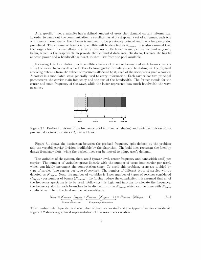
Figure 3.1: Prefixed division of the frequency pool into beams (shades) and variable division of theprefixed slots into 3 carriers (C, dashed lines)

Figure 3.1 shows the distinction between the prefixed frequency split defined by the problemand the variable carrier division modifiable by the algorithm. The bold lines represent the fixed bydesign frequency slots, while the dashed lines can be moved to adapt user’s demand.

The variables of the system, then, are 3 (power level, center frequency and bandwidth used) percarrier. The number of variables grows linearly with the number of users (one carrier per user),which can highly increment the computation time. To avoid this problem, users are divided bytype of service (one carrier per type of service). The number of different types of service will bedenoted as Ntypes. Now, the number of variables is 3 per number of types of services considered(Ntypes) per number of beams (Nbeams). To further reduce the complexity, it is assumed that all ofthe frequency spectrum is to be used. Following this logic and in order to allocate the frequency,the frequency slot for each beam has to be divided into the Ntypes, which can be done with Ntypes- 1 divisions. Then, the final number of variables is:

Nvar = Nbeams ·Ntypes︸ ︷︷ ︸Power allocation

+Nbeams · (Ntypes − 1)︸ ︷︷ ︸Frequency allocation

= Nbeams · (2Ntypes − 1) (3.1)

This number only depends on the number of beams allocated and the types of service considered.Figure 3.2 shows a graphical representation of the resource’s variables.

16

Bea

ms

Type of servicep11 p12 ... p1Ntypes

p21 p22 ... p2Ntypes

... ... ... ...

(a) Power allocation

Bea

ms

Type of serviceb11 b12 ... b1(Ntypes−1)

b21 b22 ... b2(Ntypes−1)

... ... ... ...

(b) Bandwidth allocation

Figure 3.2: Graphical representation of resource’s variables

3.1.2 Restrictions

Due to the limitations of on-board technology, current satellites have some restrictions regardingits resources. As it is common with modern spacecrafts, the most limiting restriction is the power.Within this restriction, two sub-restrictions must be considered:

• Total Power : The total amount of power consumed by all the beams cannot surpass a max-imum. This is directly related with the amount of energy that the satellite can absorb andstore during time. ∑

b

Pb ≤ Pmax (3.2)

• Amplifiers: For this problem, we assume that the satellite has a maximum number of ampli-fiers (Nampl) which is less than the number of beams (Nampl < Nbeams). This means thatthe beams have to be split into the amplifiers, which introduces another constraint regardingsubsets of beams and maximum amplifier power: the maximum power for all the beams inthe same amplifier cannot surpass the capacity of the amplifier.∑

b

Pb,a ≤ Pmax,a ∀ a in amplifiers (3.3)

For the bandwidth allocation, only one restriction has been considered: due to limitation intechnology, each carrier has to be allocated a minimum bandwidth. The distance between twoconsecutive divisions, then, must be higher than a threshold:

Bc > Bthreshold ∀ c in carriers (3.4)

No other restrictions have been considered, as the bandwidth, is not dependent on the satellite’spayload.

3.1.3 Metrics: Unmet Demand and Power

To define the metrics, we need to focus on the objective of the system: satisfy the user’s demandwhile minimizing the usage of resources.

17

• Required Data Rate (Rreq,u): data rate demanded by a user

• Offered Data Rate (Roff,u): data rate provided by the system to a user

Roff,u = Γ(Pu)Bu ∀ u in users (3.5)

• Met Demand (MD): system capacity demanded by the users that the system is able to provide.On the contrary, Unmet Demand (UD), a metric used in previous resource allocations studies[6], is the capacity demanded that the system is not able to provide

MD =∑u

min(Rreq,u, Roff,u) ∀ u in users (3.6)

UD =∑u

max(Rreq,u −Roff,u, 0) ∀ u in users (3.7)

Although both the MD and the UD define how ”well” the resources are allocated with respectto the users, the latter is economically more interesting, as usually companies have to compensateusers for unmet minimum requirements. Therefore, this will be one of the metrics of our system,and will allow us to compare our results with other algorithms.

Another economically interesting metric is the usage of resources, as the unused resources couldpotentially lead to serving more users and, thus, more revenues. Within our formulation, we considertwo main resources: Power and Bandwidth. While the former directly depends on the payload’scapacity, the latter is always available and its limits do not depend on the satellite. Companiesare usually more interested in reducing power, rather than reducing bandwidth, and, therefore, thetotal amount of power consumed will be the second metric of our system.

3.2 Simulation model

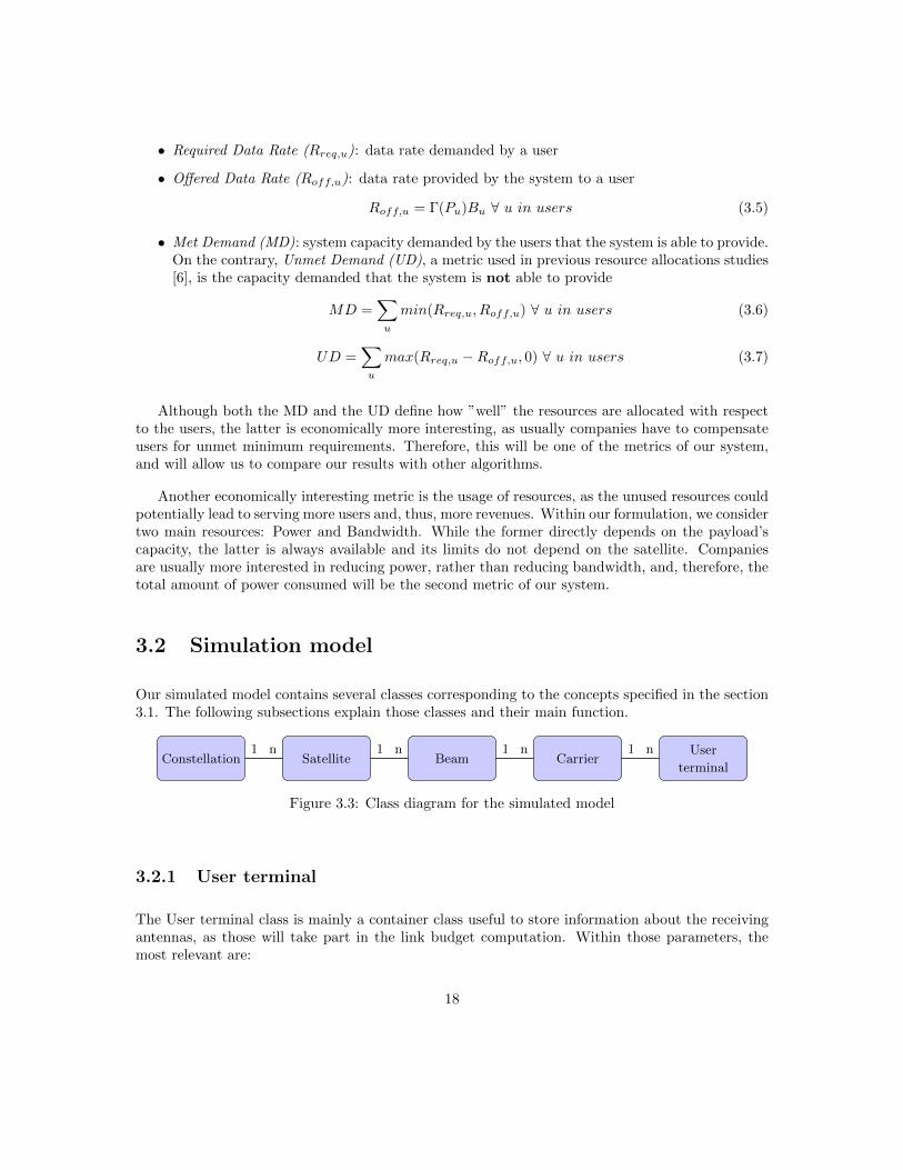
Our simulated model contains several classes corresponding to the concepts specified in the section3.1. The following subsections explain those classes and their main function.

Constellation Satellite Beam CarrierUser

terminal

1 n 1 n 1 n 1 n

Figure 3.3: Class diagram for the simulated model

3.2.1 User terminal

The User terminal class is mainly a container class useful to store information about the receivingantennas, as those will take part in the link budget computation. Within those parameters, themost relevant are:

18

• Location: useful to assign the user to a beam and the computation of distances for the linkbudget equation.

• Type of service: it determines to which carrier in the beam is going to be assigned.

• Power : how much the input signal is going to be amplified. Useful for the link budgetequation.

• Efficiency : determines a certain loss in the user’s antenna. This includes mainly electricallosses, but also depointing and degrading factors.

• Diameter : parameter of the antenna to determine the gain.

• Demand : capacity that has to be served for that user.

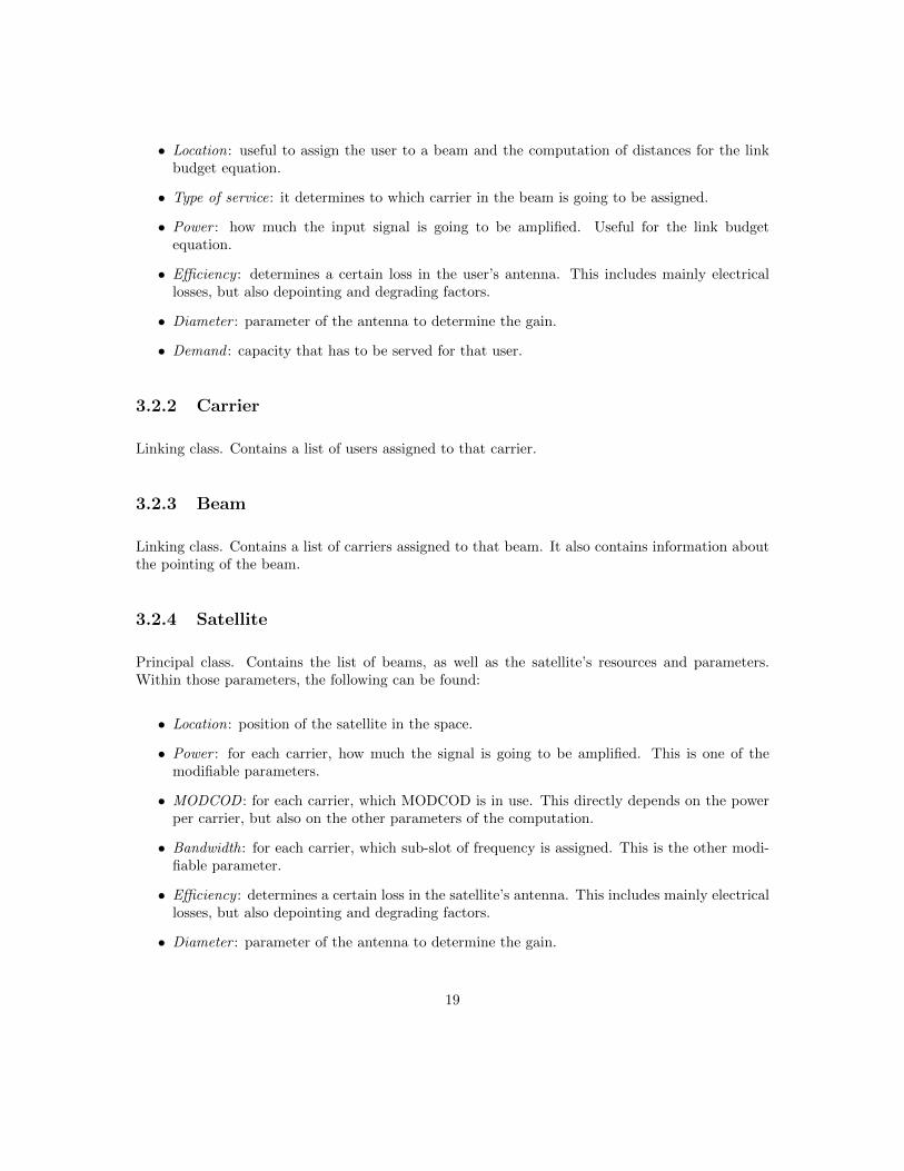
3.2.2 Carrier

Linking class. Contains a list of users assigned to that carrier.

3.2.3 Beam

Linking class. Contains a list of carriers assigned to that beam. It also contains information aboutthe pointing of the beam.

3.2.4 Satellite

Principal class. Contains the list of beams, as well as the satellite’s resources and parameters.Within those parameters, the following can be found:

• Location: position of the satellite in the space.

• Power : for each carrier, how much the signal is going to be amplified. This is one of themodifiable parameters.

• MODCOD : for each carrier, which MODCOD is in use. This directly depends on the powerper carrier, but also on the other parameters of the computation.

• Bandwidth: for each carrier, which sub-slot of frequency is assigned. This is the other modi-fiable parameter.

• Efficiency : determines a certain loss in the satellite’s antenna. This includes mainly electricallosses, but also depointing and degrading factors.

• Diameter : parameter of the antenna to determine the gain.

19

• Beams: list of beams of the satellite.

With all this information, the following functionalities can be implemented:

• Get demand : for each carrier, get the actual demand.

Rreq,carrier =∑u

Rreq,carrier,u ∀ u in users

• Get MODCOD : for each carrier and given a power, computes the quality of the link and thenthe MODCOD that is going to be used based on this quality. In the link budget equation,the MODCOD acts as a gain. Thus, knowing the SINR that has to be achieved (this is aparameter set by the operator of the satellite) allows us to compute the MODCOD.

• Get actual data rate: for each carrier, get the data rate provided. This functionality assumesthat the power and bandwidth are given. As mentioned in 2.3, the spectral efficiency is givenby the MODCOD, which depends on the power.

Roff,carrier = Γ(Pcarrier)Bcarrier

This allows us to compute the metrics explained in section 3.1.3 and give a reference on the opti-mality of the solution found.

3.2.5 Constellation

Linking class. Contains a list of satellites part of the same constellation and a list of terminals.With that information, the assignation of beams to satellites can be done. Although this thesisassumes that each beam is mapped to the nearest satellite, other mappings can be applied withoutchanging the behaviour of the algorithm.

20

Chapter 4

Metaheuristics approach

The following sections explain the algorithms implemented to solve the problem formulated insection 3.1. First, the reason behind a metaheuristic will be explained. Then, the PSO algorithmwill be theoretically presented and the practical implementation will be showed. Finally, this chapterends with a brief introduction to the GA, which will be used as a baseline to compare to in theresults.

Years of research have shown that finding the optimal solution for each of the power and fre-quency allocation problems is NP-hard and hard to approximate [6] [11]. Therefore, the complexityof the problem scales highly with the number of variables, making the finding of optimal solutioninfeasible computationally for a sufficiently large number of variables. This backs the reasoningbehind a sub-optimal algorithm that allows finding a ”good enough” solution in a feasible time.

Several sub-optimal techniques have been developed throughout the years in order to solve op-timization problems. One of the most used techniques is what is called the metaheuristic approach.According to Wikipedia, ”a metaheuristic is a higher-level procedure or heuristic designed tofind, generate, or select a heuristic (partial search algorithm) that may provide a sufficiently goodsolution to an optimization problem, especially with incomplete or imperfect information orlimited computation capacity” [19]. This definition fits perfectly the type of problem describedpreviously and, thus, it is a reasonable strategy to approach the problem. Moreover, some meta-heuristics have already been successfully applied to the power allocation, frequency assignment andjoint problem [9, 6, 17].

4.1 Particle Swarm Optimization: PSO

The Particle Swarm Optimization (PSO) is a metaheuristic algorithm, first presented in [20], basedon the movement of bird flocks. In nature, bird flocks try to find the best place to land by flyingover the search space and analyzing the possible landing spots. The flight is directed by a leader,

21

whose movements determine the direction of the flight. Each bird also remembers the best placefound so far. By analyzing a sufficient portion of the search space over time, flocks are able to finda good enough landing spot. The PSO algorithm is constructed around all these ideas.

4.1.1 Flight

Analogising bird flocks, PSO algorithms are based on a set of ”birds” flying through the searchspace aiming to find the best solution. These birds are just entities able to identify solutions andmove through the space. As any movement, the flight is mainly characterized by a position andspeed. A position in the search space is equivalent to a solution and the PSO’s objective is to findthe best position. Therefore, these elements are broadly called particles due to the resemblance withtheir physical analogy. The nature of the set of particles classifies the PSO as a population-basedalgorithm.

The particles use the concepts of leader and memory to define their trajectory. The leader isassociated with the global best, which is the best particle of the set of particles. This underlies thatall the particles know the position of all the other particles in the set and move towards the bestone. This is usually a behaviour found in hives or swarms, which is the reasoning behind the usageof the latter term for a set of particles in PSO. The memory is associated with the local best, whichis the best position that that particle has found throughout time.

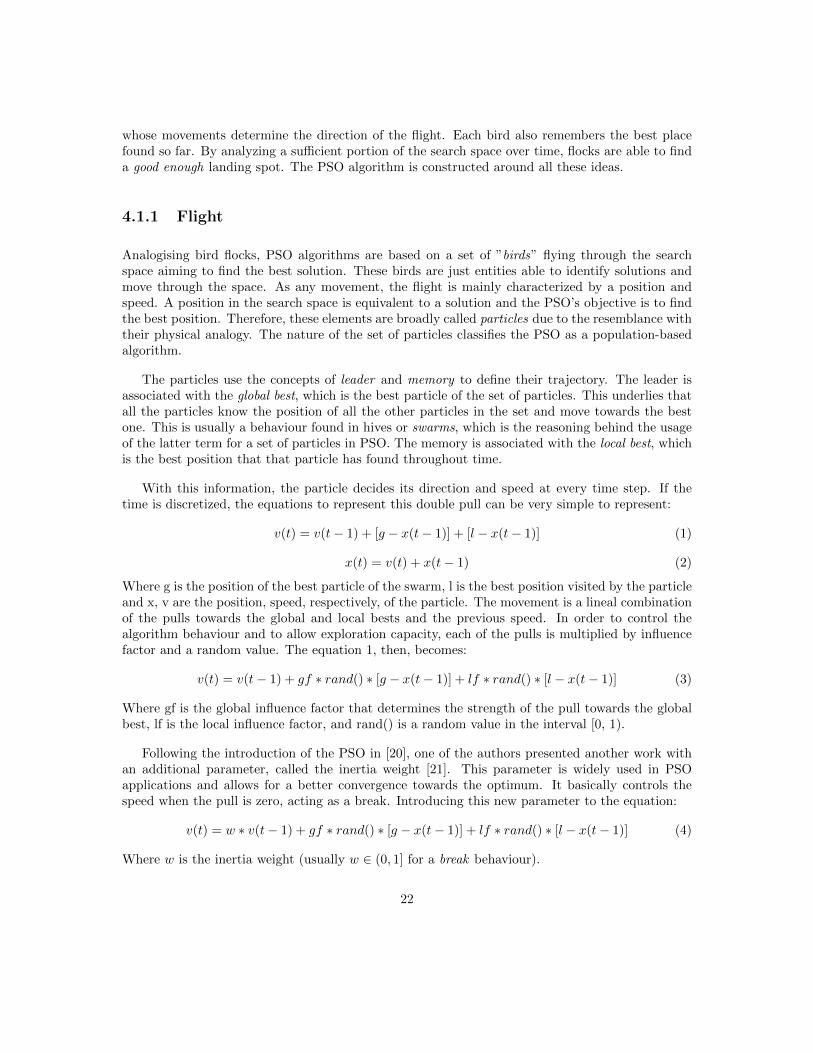
With this information, the particle decides its direction and speed at every time step. If thetime is discretized, the equations to represent this double pull can be very simple to represent:

v(t) = v(t− 1) + [g − x(t− 1)] + [l − x(t− 1)] (1)

x(t) = v(t) + x(t− 1) (2)

Where g is the position of the best particle of the swarm, l is the best position visited by the particleand x, v are the position, speed, respectively, of the particle. The movement is a lineal combinationof the pulls towards the global and local bests and the previous speed. In order to control thealgorithm behaviour and to allow exploration capacity, each of the pulls is multiplied by influencefactor and a random value. The equation 1, then, becomes:

v(t) = v(t− 1) + gf ∗ rand() ∗ [g − x(t− 1)] + lf ∗ rand() ∗ [l − x(t− 1)] (3)

Where gf is the global influence factor that determines the strength of the pull towards the globalbest, lf is the local influence factor, and rand() is a random value in the interval [0, 1).

Following the introduction of the PSO in [20], one of the authors presented another work withan additional parameter, called the inertia weight [21]. This parameter is widely used in PSOapplications and allows for a better convergence towards the optimum. It basically controls thespeed when the pull is zero, acting as a break. Introducing this new parameter to the equation:

v(t) = w ∗ v(t− 1) + gf ∗ rand() ∗ [g − x(t− 1)] + lf ∗ rand() ∗ [l − x(t− 1)] (4)

Where w is the inertia weight (usually w ∈ (0, 1] for a break behaviour).

22

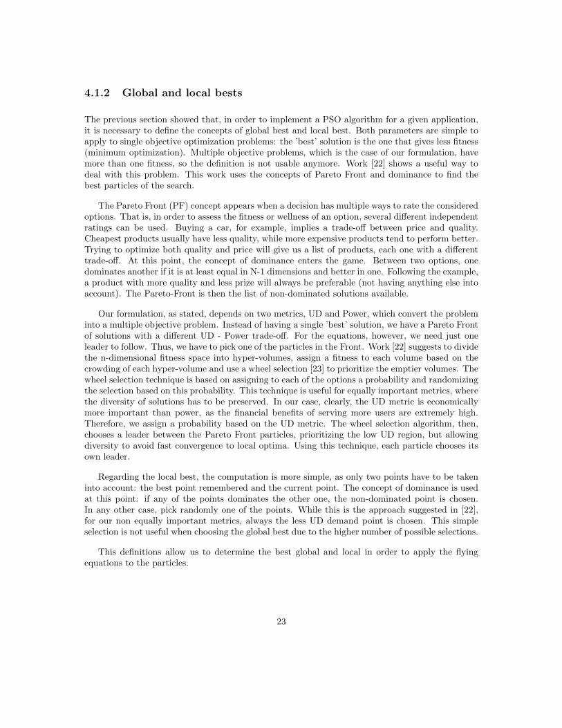
4.1.2 Global and local bests

The previous section showed that, in order to implement a PSO algorithm for a given application,it is necessary to define the concepts of global best and local best. Both parameters are simple toapply to single objective optimization problems: the ’best’ solution is the one that gives less fitness(minimum optimization). Multiple objective problems, which is the case of our formulation, havemore than one fitness, so the definition is not usable anymore. Work [22] shows a useful way todeal with this problem. This work uses the concepts of Pareto Front and dominance to find thebest particles of the search.

The Pareto Front (PF) concept appears when a decision has multiple ways to rate the consideredoptions. That is, in order to assess the fitness or wellness of an option, several different independentratings can be used. Buying a car, for example, implies a trade-off between price and quality.Cheapest products usually have less quality, while more expensive products tend to perform better.Trying to optimize both quality and price will give us a list of products, each one with a differenttrade-off. At this point, the concept of dominance enters the game. Between two options, onedominates another if it is at least equal in N-1 dimensions and better in one. Following the example,a product with more quality and less prize will always be preferable (not having anything else intoaccount). The Pareto-Front is then the list of non-dominated solutions available.

Our formulation, as stated, depends on two metrics, UD and Power, which convert the probleminto a multiple objective problem. Instead of having a single ’best’ solution, we have a Pareto Frontof solutions with a different UD - Power trade-off. For the equations, however, we need just oneleader to follow. Thus, we have to pick one of the particles in the Front. Work [22] suggests to dividethe n-dimensional fitness space into hyper-volumes, assign a fitness to each volume based on thecrowding of each hyper-volume and use a wheel selection [23] to prioritize the emptier volumes. Thewheel selection technique is based on assigning to each of the options a probability and randomizingthe selection based on this probability. This technique is useful for equally important metrics, wherethe diversity of solutions has to be preserved. In our case, clearly, the UD metric is economicallymore important than power, as the financial benefits of serving more users are extremely high.Therefore, we assign a probability based on the UD metric. The wheel selection algorithm, then,chooses a leader between the Pareto Front particles, prioritizing the low UD region, but allowingdiversity to avoid fast convergence to local optima. Using this technique, each particle chooses itsown leader.

Regarding the local best, the computation is more simple, as only two points have to be takeninto account: the best point remembered and the current point. The concept of dominance is usedat this point: if any of the points dominates the other one, the non-dominated point is chosen.In any other case, pick randomly one of the points. While this is the approach suggested in [22],for our non equally important metrics, always the less UD demand point is chosen. This simpleselection is not useful when choosing the global best due to the higher number of possible selections.

This definitions allow us to determine the best global and local in order to apply the flyingequations to the particles.

23

4.1.3 Implementation

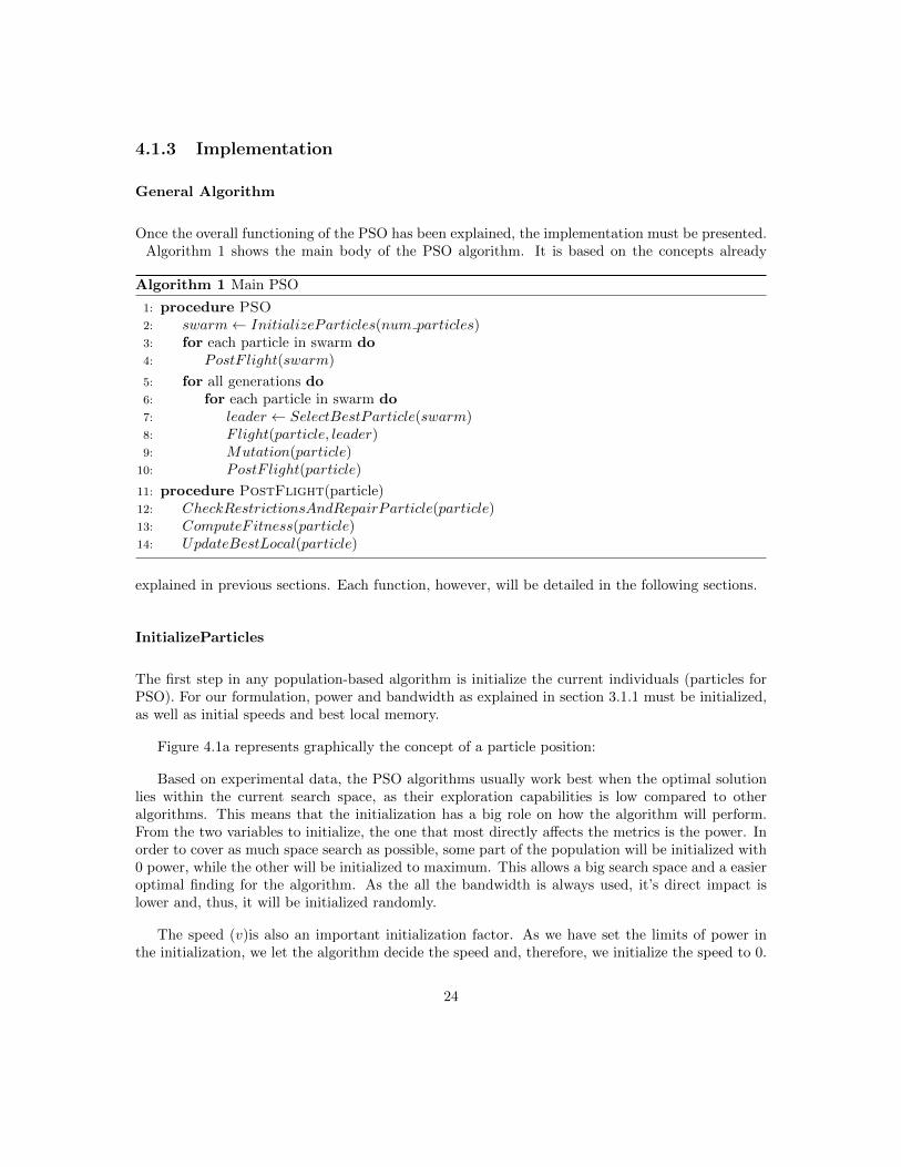
General Algorithm

Once the overall functioning of the PSO has been explained, the implementation must be presented.Algorithm 1 shows the main body of the PSO algorithm. It is based on the concepts already

Algorithm 1 Main PSO

1: procedure PSO2: swarm← InitializeParticles(num particles)3: for each particle in swarm do4: PostF light(swarm)

5: for all generations do6: for each particle in swarm do7: leader ← SelectBestParticle(swarm)8: Flight(particle, leader)9: Mutation(particle)

10: PostF light(particle)

11: procedure PostFlight(particle)12: CheckRestrictionsAndRepairParticle(particle)13: ComputeF itness(particle)14: UpdateBestLocal(particle)

explained in previous sections. Each function, however, will be detailed in the following sections.

InitializeParticles

The first step in any population-based algorithm is initialize the current individuals (particles forPSO). For our formulation, power and bandwidth as explained in section 3.1.1 must be initialized,as well as initial speeds and best local memory.

Figure 4.1a represents graphically the concept of a particle position:

Based on experimental data, the PSO algorithms usually work best when the optimal solutionlies within the current search space, as their exploration capabilities is low compared to otheralgorithms. This means that the initialization has a big role on how the algorithm will perform.From the two variables to initialize, the one that most directly affects the metrics is the power. Inorder to cover as much space search as possible, some part of the population will be initialized with0 power, while the other will be initialized to maximum. This allows a big search space and a easieroptimal finding for the algorithm. As the all the bandwidth is always used, it’s direct impact islower and, thus, it will be initialized randomly.

The speed (v)is also an important initialization factor. As we have set the limits of power inthe initialization, we let the algorithm decide the speed and, therefore, we initialize the speed to 0.

24

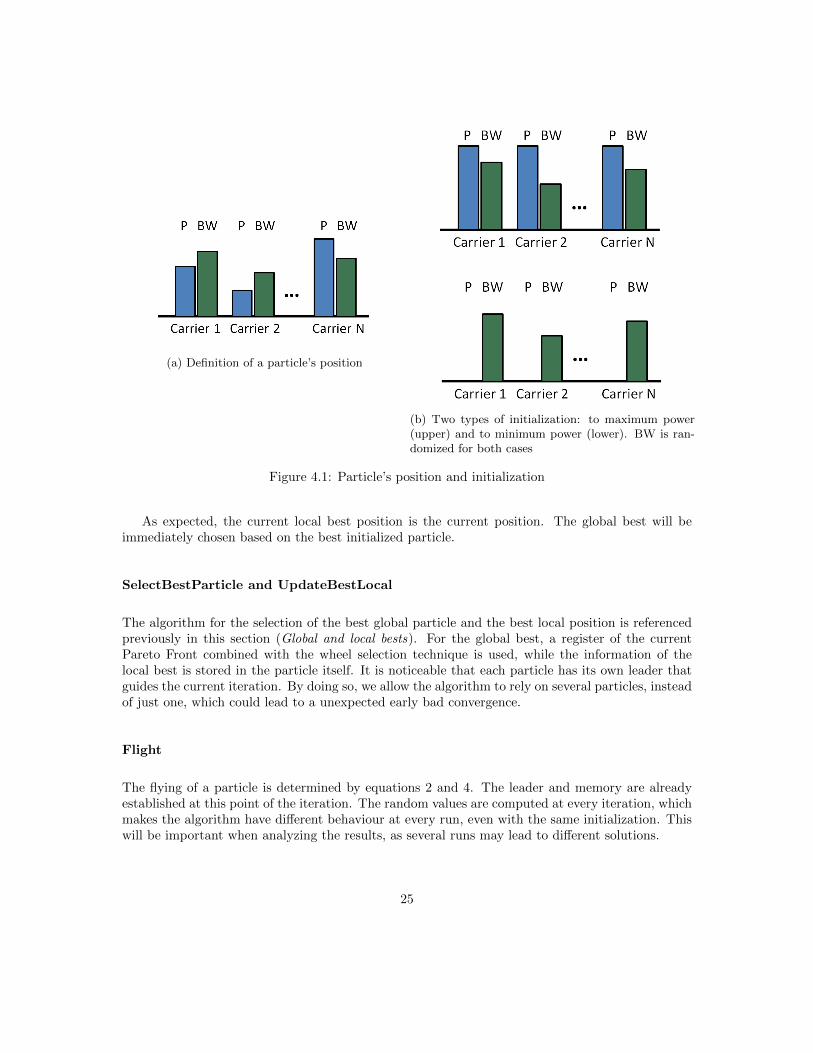
(a) Definition of a particle’s position

(b) Two types of initialization: to maximum power(upper) and to minimum power (lower). BW is ran-domized for both cases

Figure 4.1: Particle’s position and initialization

As expected, the current local best position is the current position. The global best will beimmediately chosen based on the best initialized particle.

SelectBestParticle and UpdateBestLocal

The algorithm for the selection of the best global particle and the best local position is referencedpreviously in this section (Global and local bests). For the global best, a register of the currentPareto Front combined with the wheel selection technique is used, while the information of thelocal best is stored in the particle itself. It is noticeable that each particle has its own leader thatguides the current iteration. By doing so, we allow the algorithm to rely on several particles, insteadof just one, which could lead to a unexpected early bad convergence.

Flight

The flying of a particle is determined by equations 2 and 4. The leader and memory are alreadyestablished at this point of the iteration. The random values are computed at every iteration, whichmakes the algorithm have different behaviour at every run, even with the same initialization. Thiswill be important when analyzing the results, as several runs may lead to different solutions.

25

CheckRestrictionsAndRepairParticle

This function refers to the restriction explained in section 3.1.2. Before computing the new fitness,the correctness of the current state must be validated. If the position is not valid, it has to berepaired. In our approach, we consider the following non-valid rules:

• Out of limits (Equation 3.2): the position is above the maximum or below the minimum poweror bandwidth. In the formulation, it can be seen that the power is limited by the satellite,being 0 the minimum and the maximum amplifier capacity the maximum. The bandwidth isjust a slot that has to be subdivided, while the variables are the position of the subdivision.By normalizing, the bandwidth can be clamped to the [0, 1] interval.

• Amplifier (Equation 3.3): for each amplifier, the maximum capacity cannot be surpassed. Ifthat’s the case, all the carrier’s powers within that amplifier are reduced proportionally untilthe maximum is reached.

• Bandwidth minimum distance (Equation 3.4): due to the limitations in current technology,even if the demand is 0, some resources have to be assigned to the carrier to maintain theconnection. Therefore, a sub bandwidth slot of 0 is not possible. If that’s the case, we reducethe neighboring slots to allow a minimum bandwidth for every carrier.

ComputeFitness

Using the class and function explained in section 3.2.4, both the metrics of the particle can be easilycomputed. The particles can then be rated and the Pareto Front can easily be found.

Mutation

Although it is not broadly used in PSO applications, our implementation includes a particle mu-tation [24]. This type of function allows for a better exploration, as allow the particles to get outof the current exploration zone. In our case, the mutation function simply changes some of thepositions randomly, aiming for a broader search.

4.1.4 Heuristics

Until this point, almost no information about the problem has been used in the implementation ofthe algorithm. In order to improve the performance of the PSO, some directives can be implementedto help reduce the search space and decrease convergence runtime.

From the problem, it is known that, for a specific carrier, a decrease in power or bandwidthimplies a decrease in data rate. As the UD directly depends on this factor, a decrease in datarate may imply an increase in UD. Therefore, in order to achieve higher data rates, we have to

26

increase the resources allocated for that carrier. This can be used in the flight function to guidethe flight. In our implementation, if a specific carrier has some UD, we do not allow to decreasethe power nor bandwidth. This directly means that the speed of the variables related to thatcarrier cannot allow the decrease in resources. On the other hand, if the UD is zero, the resourcesmay be excessively allocated. Then we don’t allow allocating more resources for that carrier. Thisimplementation favors the reduction of both metrics, putting more emphasis in the UD, which isof higher relevance.

4.1.5 Parameter selection

Once the algorithm’s functions have been defined, the different parameters that control the be-haviour must be decided:

• Global Influence Factor (gf): As suggested by the original PSO implementation [20], thisfactor has a value of 2. The reasoning behind this number is the equiprobability of notarriving to the point and surpassing the point, allowing some exploration capabilities.

• Local Influence Factor (lf): For the same reasons behind the gf, this factor has a value of 2.Also, neither the global best nor the local best should be prioritized in front of the other.Thus, both influence factors should be kept equal.

• Inertia Weight (w): This factor has been assigned a value of 0.729844 after the comparisonmade in [25], which states this value as the best convergence value.

• Maximum speed : In order to allow some degree of exploration, we clamp the maximum speedof the algorithm to certain limits. By doing so, we avoid getting stuck in the initializationvalues, and enforce a minimum exploration before convergence. For power, the limit is set to2.5% of the maximum power, for bandwidth, the limit is set to 5% of the maximum bandwidth.

• Mutation probability : This states the probability of a single variable of mutating. For ourimplementation, we have set this value to 0.0625% allowing the change of only a few variablesevery iteration.

4.2 Genetic Algorithm: GA

This section is intended to give a brief description of the GA and its application to this problem.As the GA is not the main topic of this thesis, just the general concepts will be explained.

The Genetic Algorithm (GA), also known as Evolutionary Algorithm, is a metaheuristic, population-based algorithm built around the evolution of living populations. Throughout time, populationssuffer from different effects that lead to better and stronger individuals, able to better fit in thecurrent environment. The GA uses those functions to evolve the set of solutions and improve themtowards the global optimum.

27

Within those functions, three are commonly found:

• Selection: The population only supports a maximum number of individuals. Thus, creatingnew individuals imply that some part of the population will be erased in order to leave place tothe new generation. Due to the multiple objectives, the Pareto Front and dominance conceptsreappear at this point.

• Mating : Following the reasoning behind animal population, the way to create new individualsis based on the mating within the current population: two individuals create another bycrossing its characteristics. The new individual has characteristics from both creators.

• Mutation: Individuals can also create another individual by randomly mutating some of itscharacteristics.

In the algorithm, the mating and mutating functions allow the population to evolve, while theselection ensures the convergence to the best solutions (a.k.a. global optimum).

The implementation of the Genetic Algorithm in this thesis is a similar approach as the presentedin [17]. To this algorithm, the heuristic presented in section 4.1.4 has been added.

28

Chapter 5

Results

This chapter aims to present the results obtained with the explained algorithms. First, the simula-tion data will be described. Then, the results for several scenarios will be provided and discussed.

5.1 Traffic model

All the analysis in this thesis are based on the traffic model provided by SES S.A., which representsa distribution of beams across America. This model contains information about a set of beams,including position, user’s antenna characteristics, maximum demand (SLA),... It contains all thenecessary physical characteristics to compute the link budget equation. A part from this spatialmodel, it also includes a temporal model, with the demand per type of service every 5 minutes fora 24h period.

The set contains 160 beams, distributed along America within ±65o latitude. With this distri-bution, we consider several demand cases based on the number of type of services considered. Atmaximum, the model considers 4 different types of services, which will be referred as A, B, C andD. In terms of demand, A<B<C<D. Considering the demand in each beam, taking 1 or 2 types(e.g. A or AB) can be stated as low demand, where the user’s requirements are always met and theUD is zero. Taking 3 types (e.g. ABC) is stated as balanced demand, where the user’s requirementsare vastly met and the UD is near zero. Finally, excess demand is understood as taking all 4 of thetypes (e.g. ABCD) and the requirements are not met. The algorithms try to minimize UD, butnever reaches 0.

Each beam has its own prefixed frequency slot defined by the model. The frequency slot dis-tribution tries to minimize the interference between the beams. As it is constrained by the model,the algorithm cannot change this distribution. The carriers, however, receive a sub-slot of thebandwidth assigned to the beam and that is one of the variables considered in the problem andchangeable by the algorithm.

29

5.2 Simulation parameters

This section presents the values of the parameters chosen for each algorithm.

Parameter Value

Swarm size 500Global factor 2Local factor 2

Power max speed 2.5%Bandwidth max speed 5%Mutation probability 15%

Variables mutated 1/16%

(a) PSO parameter selection

Parameter Value

Population size 100Crossing probability 75%

Gens crossed 60%Alpha blending (crossing) 20%

Mutation probability 15%Gens mutated 2%

(b) GA parameter selection

Table 5.1: PSO and GA parameter selection

5.3 Scenario 1: Power allocation

This first scenario presents a basic concept test of the algorithms and a general overview of theirperformance in the described problem. In order to assess the performance of the algorithms, onlythe power will be allocated, and the bandwidth will split among the carriers based on the user’smaximum contracted demand, as for this case an optimal power allocation can be found. Both thePSO and the GA will be compared with this baseline. For the results, the power will be normalizedto the optimal power, while the UD will be normalized to the total demand.

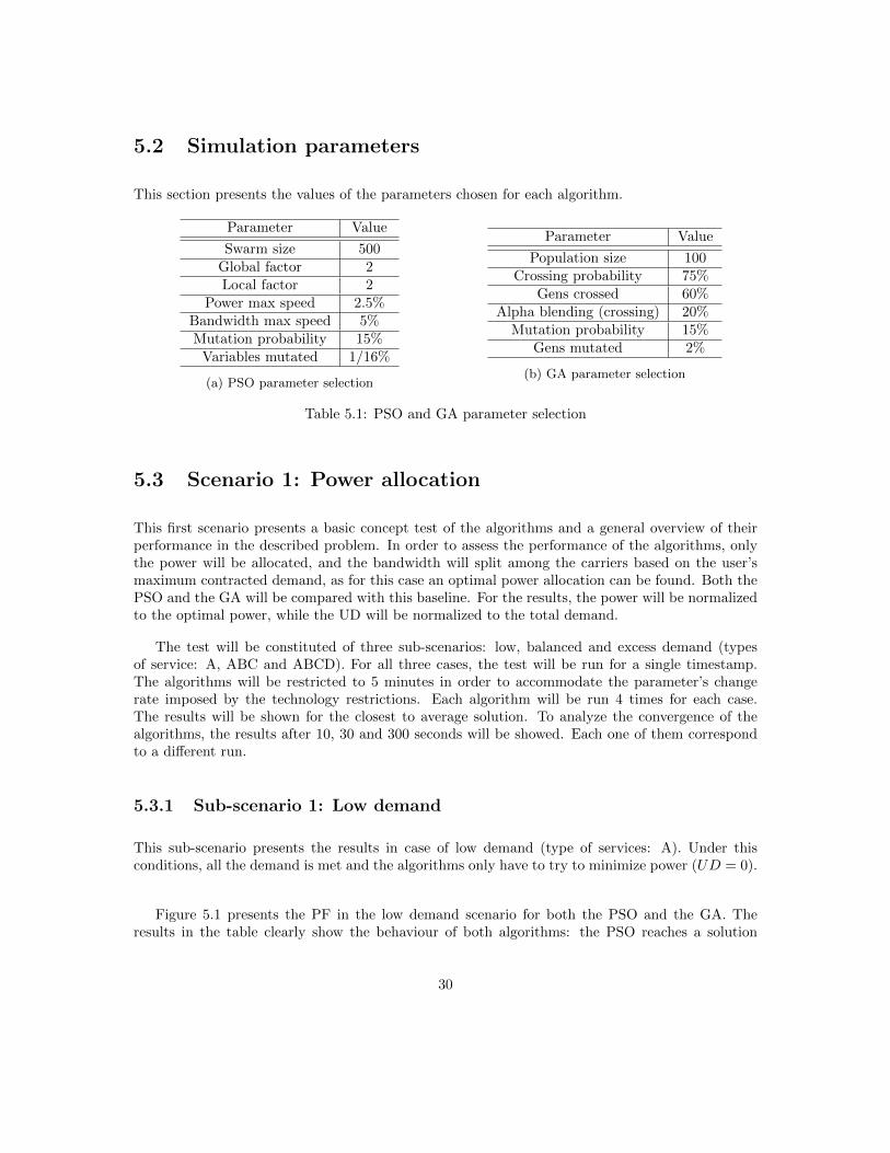
The test will be constituted of three sub-scenarios: low, balanced and excess demand (typesof service: A, ABC and ABCD). For all three cases, the test will be run for a single timestamp.The algorithms will be restricted to 5 minutes in order to accommodate the parameter’s changerate imposed by the technology restrictions. Each algorithm will be run 4 times for each case.The results will be shown for the closest to average solution. To analyze the convergence of thealgorithms, the results after 10, 30 and 300 seconds will be showed. Each one of them correspondto a different run.

5.3.1 Sub-scenario 1: Low demand

This sub-scenario presents the results in case of low demand (type of services: A). Under thisconditions, all the demand is met and the algorithms only have to try to minimize power (UD = 0).

Figure 5.1 presents the PF in the low demand scenario for both the PSO and the GA. Theresults in the table clearly show the behaviour of both algorithms: the PSO reaches a solution

30

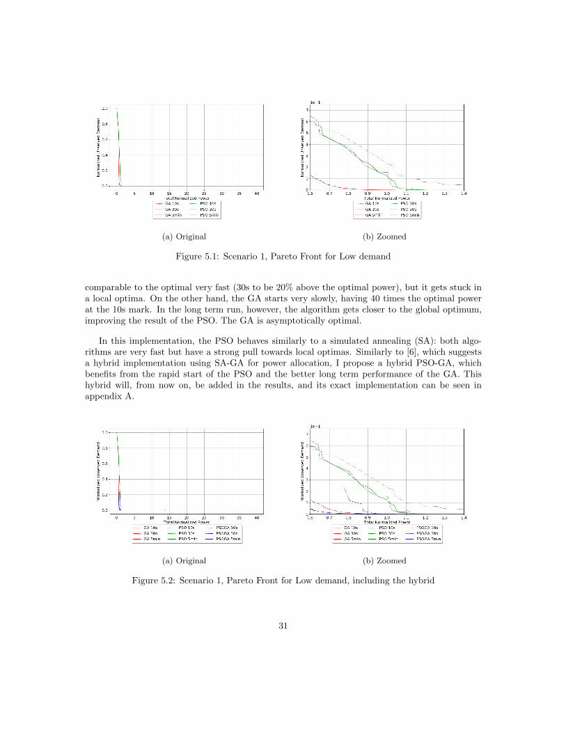
(a) Original (b) Zoomed

Figure 5.1: Scenario 1, Pareto Front for Low demand

comparable to the optimal very fast (30s to be 20% above the optimal power), but it gets stuck ina local optima. On the other hand, the GA starts very slowly, having 40 times the optimal powerat the 10s mark. In the long term run, however, the algorithm gets closer to the global optimum,improving the result of the PSO. The GA is asymptotically optimal.

In this implementation, the PSO behaves similarly to a simulated annealing (SA): both algo-rithms are very fast but have a strong pull towards local optimas. Similarly to [6], which suggestsa hybrid implementation using SA-GA for power allocation, I propose a hybrid PSO-GA, whichbenefits from the rapid start of the PSO and the better long term performance of the GA. Thishybrid will, from now on, be added in the results, and its exact implementation can be seen inappendix A.

(a) Original (b) Zoomed

Figure 5.2: Scenario 1, Pareto Front for Low demand, including the hybrid

31

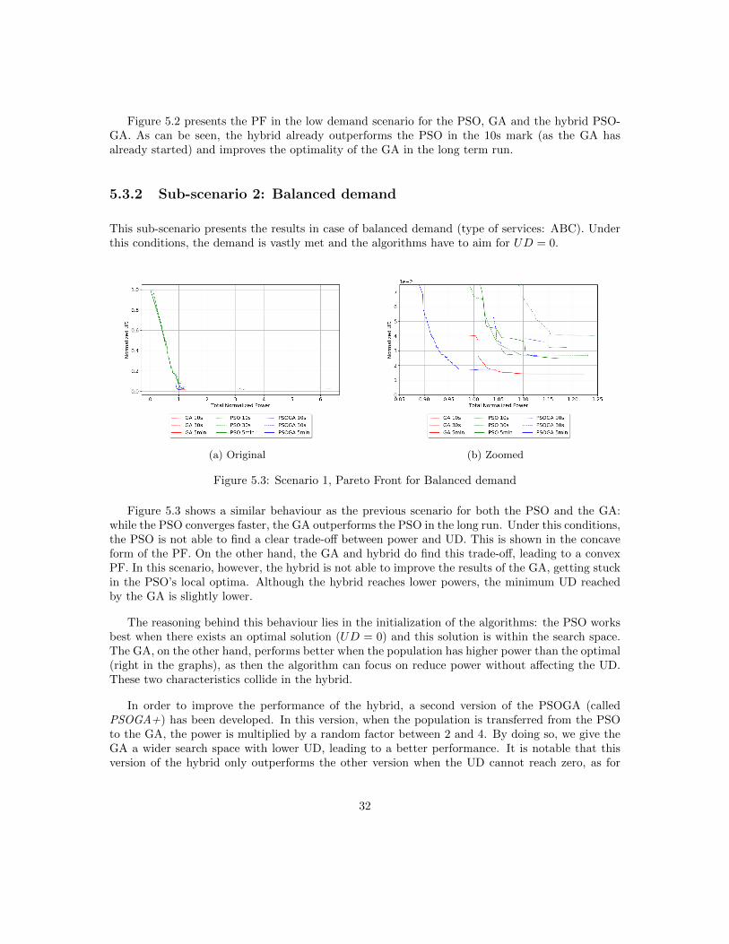
Figure 5.2 presents the PF in the low demand scenario for the PSO, GA and the hybrid PSO-GA. As can be seen, the hybrid already outperforms the PSO in the 10s mark (as the GA hasalready started) and improves the optimality of the GA in the long term run.

5.3.2 Sub-scenario 2: Balanced demand

This sub-scenario presents the results in case of balanced demand (type of services: ABC). Underthis conditions, the demand is vastly met and the algorithms have to aim for UD = 0.

(a) Original (b) Zoomed

Figure 5.3: Scenario 1, Pareto Front for Balanced demand

Figure 5.3 shows a similar behaviour as the previous scenario for both the PSO and the GA:while the PSO converges faster, the GA outperforms the PSO in the long run. Under this conditions,the PSO is not able to find a clear trade-off between power and UD. This is shown in the concaveform of the PF. On the other hand, the GA and hybrid do find this trade-off, leading to a convexPF. In this scenario, however, the hybrid is not able to improve the results of the GA, getting stuckin the PSO’s local optima. Although the hybrid reaches lower powers, the minimum UD reachedby the GA is slightly lower.

The reasoning behind this behaviour lies in the initialization of the algorithms: the PSO worksbest when there exists an optimal solution (UD = 0) and this solution is within the search space.The GA, on the other hand, performs better when the population has higher power than the optimal(right in the graphs), as then the algorithm can focus on reduce power without affecting the UD.These two characteristics collide in the hybrid.

In order to improve the performance of the hybrid, a second version of the PSOGA (calledPSOGA+) has been developed. In this version, when the population is transferred from the PSOto the GA, the power is multiplied by a random factor between 2 and 4. By doing so, we give theGA a wider search space with lower UD, leading to a better performance. It is notable that thisversion of the hybrid only outperforms the other version when the UD cannot reach zero, as for

32

this case the PSO reaches a local optima and constricts the search space of the GA.

(a) Original (b) Zoomed

Figure 5.4: Scenario 1, Pareto Front for Balanced demand, including the PSOGA+

It can be seen in figure 5.4 that the PSOGA+ reaches an UD comparable to the GA, whilereducing the power. For higher UD, however, version 1 of the hybrid outperforms version 2, as theinitialization proposed inherently increases power.

5.3.3 Sub-scenario 3: Excess demand

This sub-scenario presents the results in case of excess demand (type of services: ABCD). Underthis conditions, the demand is vastly met, but UD = 0 is unreachable, so the algorithms must tryto reduce it as much as possible.

(a) Original (b) Zoomed

Figure 5.5: Scenario 1, Pareto Front for Excess demand

33

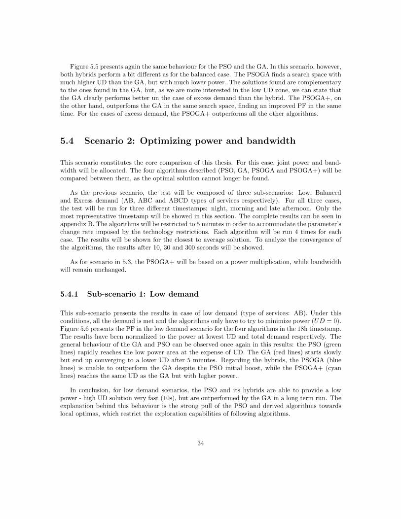
Figure 5.5 presents again the same behaviour for the PSO and the GA. In this scenario, however,both hybrids perform a bit different as for the balanced case. The PSOGA finds a search space withmuch higher UD than the GA, but with much lower power. The solutions found are complementaryto the ones found in the GA, but, as we are more interested in the low UD zone, we can state thatthe GA clearly performs better un the case of excess demand than the hybrid. The PSOGA+, onthe other hand, outperfoms the GA in the same search space, finding an improved PF in the sametime. For the cases of excess demand, the PSOGA+ outperforms all the other algorithms.

5.4 Scenario 2: Optimizing power and bandwidth

This scenario constitutes the core comparison of this thesis. For this case, joint power and band-width will be allocated. The four algorithms described (PSO, GA, PSOGA and PSOGA+) will becompared between them, as the optimal solution cannot longer be found.

As the previous scenario, the test will be composed of three sub-scenarios: Low, Balancedand Excess demand (AB, ABC and ABCD types of services respectively). For all three cases,the test will be run for three different timestamps: night, morning and late afternoon. Only themost representative timestamp will be showed in this section. The complete results can be seen inappendix B. The algorithms will be restricted to 5 minutes in order to accommodate the parameter’schange rate imposed by the technology restrictions. Each algorithm will be run 4 times for eachcase. The results will be shown for the closest to average solution. To analyze the convergence ofthe algorithms, the results after 10, 30 and 300 seconds will be showed.

As for scenario in 5.3, the PSOGA+ will be based on a power multiplication, while bandwidthwill remain unchanged.

5.4.1 Sub-scenario 1: Low demand

This sub-scenario presents the results in case of low demand (type of services: AB). Under thisconditions, all the demand is met and the algorithms only have to try to minimize power (UD = 0).Figure 5.6 presents the PF in the low demand scenario for the four algorithms in the 18h timestamp.The results have been normalized to the power at lowest UD and total demand respectively. Thegeneral behaviour of the GA and PSO can be observed once again in this results: the PSO (greenlines) rapidly reaches the low power area at the expense of UD. The GA (red lines) starts slowlybut end up converging to a lower UD after 5 minutes. Regarding the hybrids, the PSOGA (bluelines) is unable to outperform the GA despite the PSO initial boost, while the PSOGA+ (cyanlines) reaches the same UD as the GA but with higher power..

In conclusion, for low demand scenarios, the PSO and its hybrids are able to provide a lowpower - high UD solution very fast (10s), but are outperformed by the GA in a long term run. Theexplanation behind this behaviour is the strong pull of the PSO and derived algorithms towardslocal optimas, which restrict the exploration capabilities of following algorithms.

34

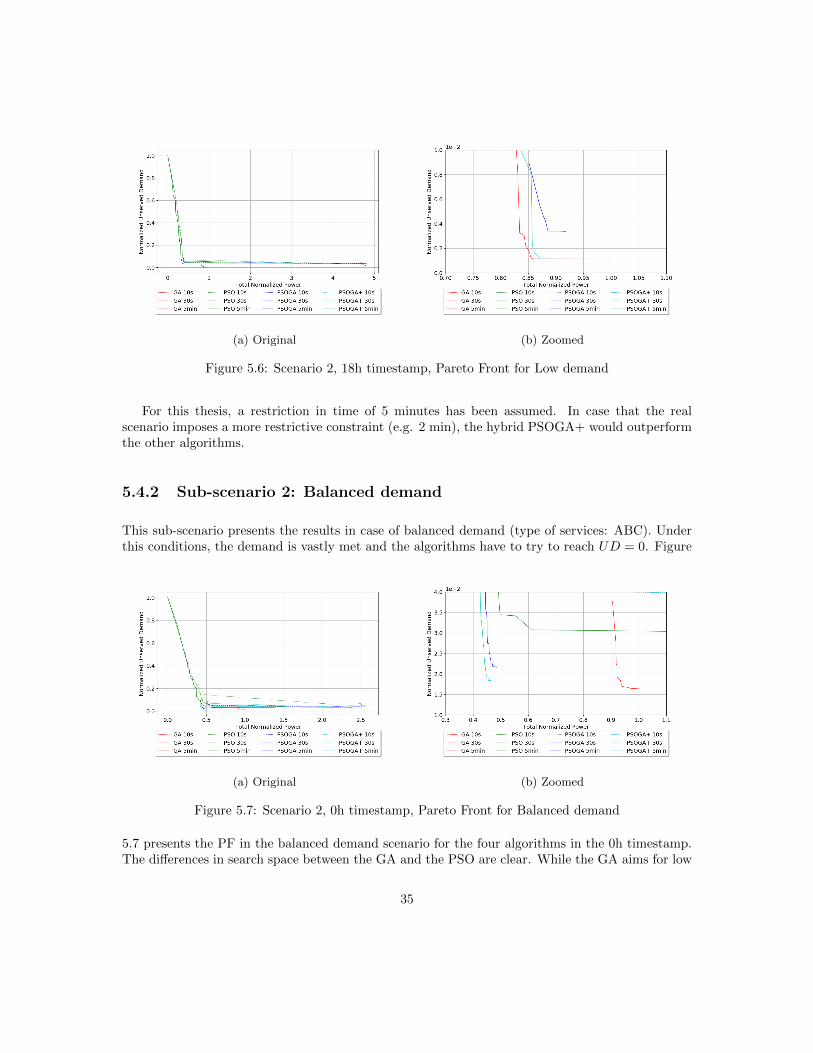
(a) Original (b) Zoomed

Figure 5.6: Scenario 2, 18h timestamp, Pareto Front for Low demand

For this thesis, a restriction in time of 5 minutes has been assumed. In case that the realscenario imposes a more restrictive constraint (e.g. 2 min), the hybrid PSOGA+ would outperformthe other algorithms.

5.4.2 Sub-scenario 2: Balanced demand

This sub-scenario presents the results in case of balanced demand (type of services: ABC). Underthis conditions, the demand is vastly met and the algorithms have to try to reach UD = 0. Figure

(a) Original (b) Zoomed

Figure 5.7: Scenario 2, 0h timestamp, Pareto Front for Balanced demand

5.7 presents the PF in the balanced demand scenario for the four algorithms in the 0h timestamp.The differences in search space between the GA and the PSO are clear. While the GA aims for low

35

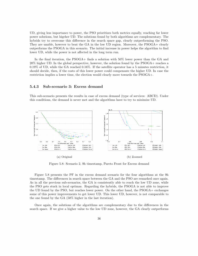
UD, giving less importance to power, the PSO prioritizes both metrics equally, reaching far lowerpower solutions, but higeher UD. The solutions found by both algorithms are complementary. Thehybrids try to overcome this difference in the search space gap, clearly outperforming the PSO.They are unable, however to beat the GA in the low UD region. Moreover, the PSOGA+ clearlyoutperforms the PSOGA in this scenario. The initial increase in power helps the algorithm to findlower UD, while the power is not affected in the long term run.

In the final iteration, the PSOGA+ finds a solution with 50% lower power than the GA and20% higher UD. In the global perspective, however, the solution found by the PSOGA+ reaches a0.19% of UD, while the GA reached 0.16%. If the satellite operator has a 5 minutes restriction, itshould decide, then, if the costs of this lower power could compensate the higher UD. In case therestriction implies a lower time, the election would clearly move towards the PSOGA+.

5.4.3 Sub-scenario 3: Excess demand

This sub-scenario presents the results in case of excess demand (type of services: ABCD). Underthis conditions, the demand is never met and the algorithms have to try to minimize UD.

(a) Original (b) Zoomed

Figure 5.8: Scenario 2, 9h timestamp, Pareto Front for Excess demand

Figure 5.8 presents the PF in the excess demand scenario for the four algorithms at the 9htimestamp. The differences in search space between the GA and the PSO are remarked once again.As in all the previous sub-scenarios, the GA is consistently able to reach the low UD zone, whilethe PSO gets stuck in local optimas. Regarding the hybrids, the PSOGA is not able to improvethe UD found by the PSO, but reaches lower power. On the other hand, the PSOGA+ exchangessome of this power improvements to get lower UD. This lower UD, however, is not comparable tothe one found by the GA (50% higher in the last iteration).

Once again, the solutions of the algorithms are complementary due to the differences in thesearch space. If we give a higher value to the low UD zone, however, the GA clearly outperforms

36

all the other algorithms, including the hybrids, in the long term run.

37

Chapter 6

Conclusions

This chapter summarizes the main findings of this thesis and introduces possible future works toimprove the results presented in this document.

6.1 Conclusions and remarks

This thesis presents a PSO and two hybrids PSOGA implementations to solve the RA problem insatellite communications. First, the motivation and objectives of this work have been presented.Second, the satellite communications context has been introduced. Third, the problem has beenformulated and the simulation model has been explained. Fourth, the implementation of the PSOhas been shown and, finally, the results for the PSO, the baseline GA and the hybrids have beendiscussed.

As a first remark, the PSO is a suitable algorithm to solve the dynamic resource managementproblem in High-Throughput Multi-beam satellite systems and can be successfully implemented ina real-case application.

For power and joint power and bandwidth allocation, the PSO has a very fast convergence (15 to20 iterations, 12 - 15s for 500 particles) towards a local optima. The results show big improvementsin early stages with respect to a standard implementation of a GA. The latter, however, consistentlyoutperforms the PSO in the long term run.

Both the characteristics of the PSO and the GA can be unified in a hybrid PSOGA. The PSOGAand variants clearly outperform both the PSO and the GA in the problem of power allocation,reaching lower UD regions.

For the joint power and bandwidth allocation problems, the hybrid algorithms are able toreduce highly (up to 50%) the power consumption, at the expense of an up to 50% increase in UD

38

in the worst case, compared with the sole GA execution in the 5 min mark. In a 30s execution,however, the PSO and hybrids reach an 80% power reduction, while achieving 2% lower UD, clearlyoutperforming the GA.

6.2 Future work

This thesis has introduced the formulation and implementation of the Particle Swarm Optimizationmethod to the joint power and bandwidth allocation subproblem inside the Dynamic ResourceManagement problem for satellite communications. Possible extensions of the work presented inthis thesis may cover:

• Inclusion of the frequencies flexibilities for modern constellations: while this thesis worksunder a frequency fixed model, modern constellations allow to change the frequency perbeam, variable that could potentially be included in the algorithm as a decision variable.

• Inclusion of other subproblems inside the RA problem: this thesis presents the implementationof the joint power and bandwidth allocation problem. Other subproblems inside the RA, suchas the beam placement and beam shape could also be included in the decision variables ofthe algorithm.

• PSO and hybrids heuristic improvements: while this thesis works with the presented imple-mentation of the algorithms, further improvements in the algorithms could reach significantbetter results.

• Robustness and size sensitivity analyses: to further understand the behaviour and advantagesof all algorithms.

• Parameter tuning: while for this thesis, the parameter selection has followed an ad hoc proce-dure based on the results obtained, a further work could include a better parameter refiningto increase the performance of the PSO and hybrids.

39

Appendices

40

Appendix A

PSO-GA: a hybrid approach

In general terms, the PSO is a fast optimization technique with low exploration capabilities. Thistends to lead the algorithm to a local optima solution. On the other hand, the GA is a slowerconvergence technique with high exploration and exploitation capabilities. This leads to a globaloptimum at the cost of computation time. These characteristics suggest for a hybrid algorithm,able to combine the fastness of the PSO and the exploration of the GA to converge faster to theglobal optimum.

A.1 Implementation of a PSO-GA

We envision this hybrid as a two step process: first, a fast PSO execution to obtain a better startingpoint for the GA and then a long GA run to reach the expected convergence of the algorithm. Basedon this, our implementation is based on a 10-iteration PSO run followed by the GA. The explanationof this 10-iteration concept is detailed in the following lines.

Figure A.1 shows the PSO fast convergence. In very few iterations, the algorithm provides agood enough solution. This value, however, is a local optima, and the algorithm gets stuck in there.For this reason, the starting point of the GA should not be the convergence value of the PSO, butrather a previous step, before entering the local optima. The 10th iteration is a good compromisebetween a far from optimal solution and a local optima solution.

Although the transfer of population between the two algorithms is simple due to the nature ofthe implementations, the search space has to be taken into account. In our formulation, the UDis more important than the power consumed. While both metrics are interesting from the point ofview of the algorithm, the low power - high UD region is not interesting from the financial point ofview. Thus, the interest region will be around the low UD region. While the PSO has not troublewhen dealing with a big search space, the exploitation capabilities of the GA make the algorithmperform better in an enclosed small region. Therefore, when transfering from the PSO to the GA,

41

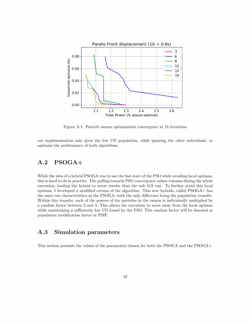
Figure A.1: Particle swarm optimization convergence in 18 iterations

our implementation only gives the low UD population, while ignoring the other individuals, tooptimize the performance of both algorithms.

A.2 PSOGA+

While the idea of a hybrid PSOGA was to use the fast start of the PSO while avoiding local optimas,this is hard to do in practice. The pulling towards PSO convergence values remains during the wholeexecution, leading the hybrid to worst results than the sole GA run. To further avoid this localoptimas, I developed a modified version of the algorithm. This new hybrids, called PSOGA+ hasthe same run characteristics as the PSOGA, with the only difference being the population transfer.Within this transfer, each of the powers of the particles in the swarm is individually multiplied bya random factor between 2 and 4. This allows the execution to move away from the local optimaswhile maintaining a sufficiently low UD found by the PSO. This random factor will be denoted aspopulation modification factor or PMF.

A.3 Simulation parameters

This section presents the values of the parameters chosen for both the PSOGA and the PSOGA+.

42

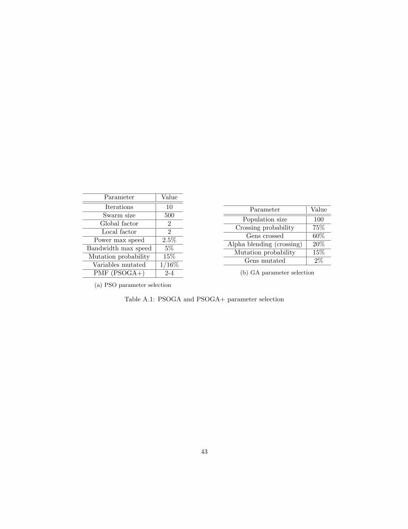
Parameter Value

Iterations 10Swarm size 500

Global factor 2Local factor 2

Power max speed 2.5%Bandwidth max speed 5%Mutation probability 15%

Variables mutated 1/16%PMF (PSOGA+) 2-4

(a) PSO parameter selection

Parameter Value

Population size 100Crossing probability 75%

Gens crossed 60%Alpha blending (crossing) 20%

Mutation probability 15%Gens mutated 2%

(b) GA parameter selection

Table A.1: PSOGA and PSOGA+ parameter selection

43

Appendix B

Scenario 2 complete results

This chapter presents the complete results for joint power and bandwidth allocation with the fouralgorithms presented.

44

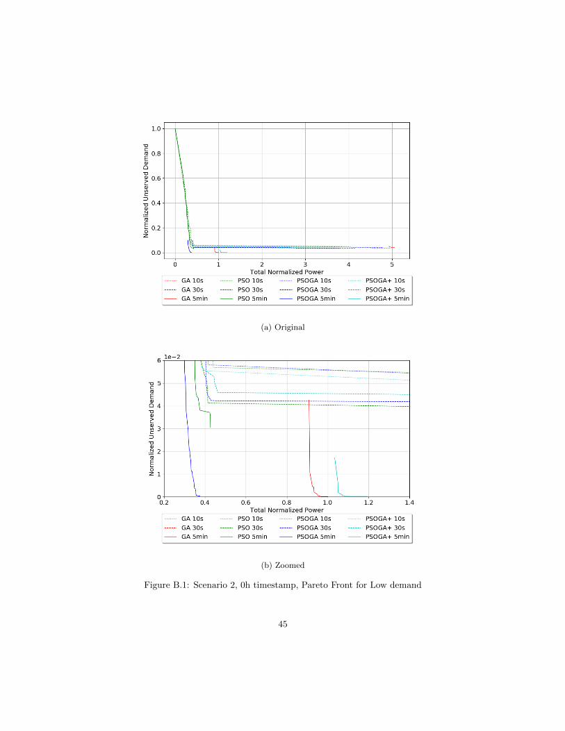
(a) Original

(b) Zoomed

Figure B.1: Scenario 2, 0h timestamp, Pareto Front for Low demand

45

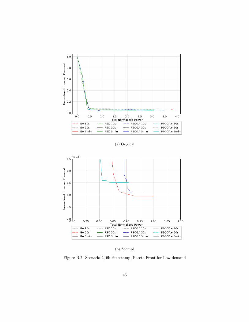
(a) Original

(b) Zoomed

Figure B.2: Scenario 2, 9h timestamp, Pareto Front for Low demand

46

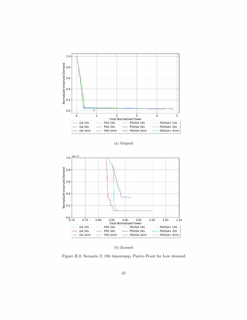
(a) Original

(b) Zoomed

Figure B.3: Scenario 2, 18h timestamp, Pareto Front for Low demand

47

(a) Original

(b) Zoomed

Figure B.4: Scenario 2, 0h timestamp, Pareto Front for Balanced demand

48

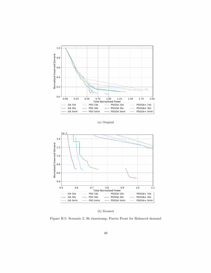
(a) Original

(b) Zoomed

Figure B.5: Scenario 2, 9h timestamp, Pareto Front for Balanced demand

49

(a) Original

(b) Zoomed

Figure B.6: Scenario 2, 18h timestamp, Pareto Front for Balanced demand

50

(a) Original

(b) Zoomed

Figure B.7: Scenario 2, 0h timestamp, Pareto Front for Excess demand

51

(a) Original

(b) Zoomed

Figure B.8: Scenario 2, 9h timestamp, Pareto Front for Excess demand

52

(a) Original

(b) Zoomed

Figure B.9: Scenario 2, 18h timestamp, Pareto Front for Excess demand

53

Bibliography

[1] E. S. Agency, “Satellite frequency bands,” 2019. Available at: https://www.esa.int/

spaceinimages/Images/2013/11/Satellite_frequency_bands Last visited: 2019-07-12.

[2] Saburchill.com, “The open door web site : Ib physics : Waves : Polarization of waves,”2019. Available at: https://www.saburchill.com/physics/chapters2/0040.html Last vis-ited: 2019-07-12.

[3] G. Maral and M. Bousquet, Satellite communications systems: systems, techniques and tech-nology. John Wiley & Sons, 2011.

[4] M. Stanley, “Space: Investment implications of the fi-nal frontier,” tech. rep., M. Stanley, 2017. Available at:https://fa.morganstanley.com/griffithwheelwrightgroup/mediahandler/media/106686/Space%20Investment%20Implications%20of%20the%20Final%20Frontier.pdf (2019/23/08).

[5] S. Networks, “Unleashing the potential of an empowered -world with the launch of o3bmpower,” tech. rep., SES, 2017. Available at: https://www.ses.com/sites/default/files/2017-09/170908 SES%20Launches%20O3b%20mPOWER FINAL.pdf (2019/23/08).

[6] A. I. Aravanis, B. S. MR, P.-D. Arapoglou, G. Danoy, P. G. Cottis, and B. Ottersten, “Powerallocation in multibeam satellite systems: A two-stage multi-objective optimization,” IEEETransactions on Wireless Communications, vol. 14, no. 6, pp. 3171–3182, 2015.

[7] H. Wang, A. Liu, X. Pan, and J. Yang, “Optimization of power allocation for multiusersin multi-spot-beam satellite communication systems,” Mathematical Problems in engineering,vol. 2014, 2014.

[8] Y. Hong, A. Srinivasan, B. Cheng, L. Hartman, and P. Andreadis, “Optimal power allocationfor multiple beam satellite systems,” in 2008 IEEE Radio and Wireless Symposium, pp. 823–826, IEEE, 2008.

[9] F. R. Durand and T. Abrao, “Power allocation in multibeam satellites based on particleswarm optimization,” AEU-International Journal of Electronics and Communications, vol. 78,pp. 124–133, 2017.

[10] J. J. G. Luis, M. Guerster, I. del Portillo, E. Crawley, and B. Cameron, “Deep reinforcementlearning architecture for continuous power allocation in high throughput satellites,” arXivpreprint arXiv:1906.00571, 2019.

54

[11] T. Mizuike and Y. Ito, “Optimization of frequency assignment,” IEEE Transactions on Com-munications, vol. 37, no. 10, pp. 1031–1041, 1989.

[12] U. Park, H. W. Kim, D. S. Oh, and B.-J. Ku, “A dynamic bandwidth allocation scheme for amulti-spot-beam satellite system,” Etri Journal, vol. 34, no. 4, pp. 613–616, 2012.

[13] H. Wang, A. Liu, X. Pan, and L. Jia, “Optimal bandwidth allocation for multi-spot-beamsatellite communication systems,” in Proceedings 2013 International Conference on Mecha-tronic Sciences, Electric Engineering and Computer (MEC), pp. 2794–2798, IEEE, 2013.

[14] X. Hu, S. Liu, R. Chen, W. Wang, and C. Wang, “A deep reinforcement learning-based frame-work for dynamic resource allocation in multibeam satellite systems,” IEEE CommunicationsLetters, vol. 22, no. 8, pp. 1612–1615, 2018.

[15] S. Salcedo-Sanz and C. Bousono-Calzon, “A hybrid neural-genetic algorithm for the frequencyassignment problem in satellite communications,” Applied Intelligence, vol. 22, no. 3, pp. 207–217, 2005.

[16] J. Lei and M. A. Vazquez-Castro, “Joint power and carrier allocation for the multibeam satel-lite downlink with individual sinr constraints,” in 2010 IEEE International Conference onCommunications, pp. 1–5, IEEE, 2010.

[17] A. Paris, I. Del Portillo, B. Cameron, and E. Crawley, “A genetic algorithm for joint powerand bandwidth allocation in multibeam satellite systems,” in 2019 IEEE Aerospace Conference,pp. 1–15, IEEE, 2019.

[18] C. E. Shannon, “A mathematical theory of communication,” Bell System Technical Journal,vol. 27, no. 3, p. 379–423, 1948.

[19] En.wikipedia.org., “Metaheuristic,” 2019. Available at: https://en.wikipedia.org/wiki/

Metaheuristic Last visited: 2019-06-24.

[20] R. Eberhart and J. Kennedy, “A new optimizer using particle swarm theory,” in MHS’95.Proceedings of the Sixth International Symposium on Micro Machine and Human Science,pp. 39–43, Ieee, 1995.

[21] Y. Shi and R. Eberhart, “A modified particle swarm optimizer,” in 1998 IEEE internationalconference on evolutionary computation proceedings. IEEE world congress on computationalintelligence (Cat. No. 98TH8360), pp. 69–73, IEEE, 1998.

[22] C. C. Coello and M. S. Lechuga, “Mopso: A proposal for multiple objective particle swarmoptimization,” in Proceedings of the 2002 Congress on Evolutionary Computation. CEC’02(Cat. No. 02TH8600), vol. 2, pp. 1051–1056, IEEE, 2002.

[23] A. Lipowski and D. Lipowska, “Roulette-wheel selection via stochastic acceptance,” PhysicaA: Statistical Mechanics and its Applications, vol. 391, no. 6, pp. 2193–2196, 2012.

[24] M. R. Sierra and C. A. C. Coello, “Improving pso-based multi-objective optimization us-ing crowding, mutation and ε-dominance,” in International conference on evolutionary multi-criterion optimization, pp. 505–519, Springer, 2005.

55

[25] J. C. Bansal, P. Singh, M. Saraswat, A. Verma, S. S. Jadon, and A. Abraham, “Inertia weightstrategies in particle swarm optimization,” in 2011 Third world congress on nature and biolog-ically inspired computing, pp. 633–640, IEEE, 2011.

56