Poverty Mapping in the Kyrgyz Republic1 - The World...

1

Poverty Mapping in the Kyrgyz Republic1

Methodology and Key Findings

Meera Mahadevan (World Bank)

Nobuo Yoshida (World Bank)

Larisa Praslova (National Statistics Committee, Kyrgyz Republic)

April, 2013

Poverty Reduction and Economic Management Unit

Europe and Central Asia Region

Document of the World Bank

1 This report is prepared by a team from the World Bank and the National Statistics Committee, Kyrgyz Republic.

This study has been conducted under an umbrella work program, “Kyrgyz Republic Poverty Analysis Program.” We

would like to thank Sarosh Satter (the Task Team Leader of the work program) for her continued guidance and

support. We gratefully acknowledge Brian Blankespoor produced all maps and provided the market accessibility

index map. We would also like to thank Aibek Balibagysh Uulu, and Aziz Atamanov for their useful comments and

suggestions. We would thankfully acknowledge two peer reviewers, Umar Serajuddin and Hai-Anh Dang, for their

insightful and constructive comments. Finally, we would like to thank Peter Lanjouw and Roy Van der Weide for

their technical advices, particularly informing us of the latest recommendations in the World Bank‟s research

department.

Disclaimer: The boundaries, colors, denominations and any other information shown on these maps do not imply, on

the part of The World Bank Group, any judgment on the legal status of any territory, or any endorsement or

acceptance of such boundaries.

Pub

lic D

iscl

osur

e A

utho

rized

Pub

lic D

iscl

osur

e A

utho

rized

Pub

lic D

iscl

osur

e A

utho

rized

Pub

lic D

iscl

osur

e A

utho

rized

Pub

lic D

iscl

osur

e A

utho

rized

Pub

lic D

iscl

osur

e A

utho

rized

Pub

lic D

iscl

osur

e A

utho

rized

Pub

lic D

iscl

osur

e A

utho

rized

wb350881

Typewritten Text

76690

2

I. Introduction 1. This report describes the process of and results from a poverty mapping exercise for the Kyrgyz

Republic, using the Kyrgyz Integrated Household Survey (KIHS 2009)2 and the Population and Housing

Census (2009).

2. Poverty mapping is an exercise to estimate poverty incidence at a level where a typical household

income and expenditure survey cannot produce statistically reliable poverty estimates due to high

sampling errors. In the Kyrgyz Republic, official poverty rates are not produced below oblast level, as the

sampling errors of the survey data become non-negligible. Various poverty mapping methodologies were

devised to overcome increasing imprecision of poverty estimates as they are disaggregated.

3. The poverty mapping methodology used for this exercise is the Small Area Estimation (SAE)

method developed by Elbers, et al. (2003). This methodology is one of the most commonly used poverty

mapping methodologies around the world and has been widely tested and validated. The method takes

advantage of the strengths of both sources: the breadth of data in the integrated survey, including

expenditure data, and the size and coverage in the Census, meaning that data were collected from all

households in the country as opposed to „sampled‟ from a primary sampling unit.

4. The goal for the poverty maps of the Kyrgyz Republic was to obtain poverty estimates at rayon or

district level, a level at which the survey is not representative. For the purposes of this poverty map, all 7

oblasts of the Kyrgyz Republic have been considered and one out of the two cities holding a similar status

to oblasts, for which data was collected in the survey.3 These include Issyk-Kul, Jalalabad, Naryn,

Batken, Osh, Talas, Chui and Bishkek city. Oblasts are further disaggregated into 40 administrative units

called “rayons” (equivalent to districts) and 13 towns4 Bishkek is also divided into 4 rayons,

5. This poverty mapping exercise has been conducted jointly with the National Statistics Committee

(NSC). The World Bank team has provided hands-on training on the poverty mapping method to the NSC

members. Since then, the NSC team and the World Bank team have continued to work together and have

cooperated on the technical and methodological aspects of the analysis.

Poverty mapping and Kyrgyzstan

6. Kyrgyzstan's landscape is blessed with a dramatic range of weather conditions and altitudes from

snow-capped peaks, dry deserts, vast grasslands, to fertile farmlands. This rich terrain supports a rich

diversity of plant and animal life. Kyrgyzstan is also rich in cultural diversity - the life style varies from a

traditional nomadic style to the modern lifestyles in Bishkek. The landscape has shaped and preserved this

nomadic lifestyle and culture for centuries while also allowing for economic growth in cities like Bishkek

and Osh. Kyrgyzstan is a land-locked country surrounded by four countries: Kazakhstan in the north,

2 We use the KIHS 2009, in spite of the availability of the KIHS 2010. The 2009 KIHS was conducted the same year as the census. Poverty

mapping involves the assumption that the parameters of the consumption model remain constant between the survey and the census, and only the

household variables change. This assumption holds true if the survey and the census are from the same year, and this is usually given the highest preference. 3 The Government of the Kyrgyz Republic has identified Bishkek and Osh City as cities with “republican subordination” which, in effects, gives

these two cities oblast status. 4 Throughout the report the term rayon is used both for towns and rayon for brevity.

3

China to the east and south-east, Tajikistan to the south-west and Uzbekistan to the west. Trade with these

countries shapes economic opportunities for border areas.

7. Poverty mapping is useful for a country with strong regional diversity. For example, Atamanov et

al. (forthcoming) suggests discernible welfare disparities between the capital city of Bishkek and the rural

and urban areas in the rest of the country. It shows that educational attainment and household

demographics differ significantly depending on the area of residence. Such diversities can be observed

even among rural areas. The rural areas of Chui (in relatively close proximity to the capital, Bishkek)

appear to enjoy significantly better living standards than rural areas in the rest of the country.

8. National poverty rates alone cannot tell us the living standards faced by people in different parts

of the country. Disaggregated poverty indicators will help policy makers provide resources to the areas

that need it the most in an objective and transparent manner. Besides poverty maps, Kyrgyzstan has other

rich geo-referenced databases which include rayon level public expenditure data created by the

government of Kyrgyzstan and the World Bank.

Figure 1: Administrative Map of Kyrgyzstan

Source: nationsonline.org

4

Figure 2: Elevation Map of Kyrgyzstan

Source: SRTM5

II. Methodology and Data

II.1. Methodology

9. The selection of the specific poverty mapping methodology is critical; numerous methods are

available and have been documented by Bigman and Deichmann (2000). An SAE method developed by

Elbers et al. (2003) (henceforth referred to as ELL) has gained wide popularity amongst development

practitioners around the world.

10. This Kyrgyz poverty map adopted the SAE method developed by ELL. It imputes consumption

levels into census households based on a consumption model estimated from the household survey. In

order for this to be possible, the consumption model must include explanatory variables (household and

individual characteristics) that are available in both the census and the survey. By applying the estimated

coefficients to the “common” variables from the census data, consumption expenditures of census

households are imputed. Poverty and inequality statistics for small areas are then calculated with the

imputed consumption of census households.

11. One advantage of this method is that it not only estimates poverty incidence but also estimates

standard errors of poverty estimates. Since poverty estimates are computed based on imputed

consumption, they cannot escape imputation errors, which are their standard errors. ELL analyzed the

properties of such imputation errors in detail and derived a procedure to compute standard errors of

poverty estimates. Box 1 below provides greater detail on this method.

II.2. Main Data Sources and Issues faced

12. The ELL method generally makes use of household survey and population census data. The

Kyrgyzstan poverty map is no exception, using the unit record Kyrgyz Integrated Household Survey

5 Jarvis , A., H.I. Reuter, A. Nelson, E. Guevara, 2008, Hole-filled SRTM for the globe Version 4, available from the CGIAR-CSI SRTM 90m

Database ( http://srtm.csi.cgiar.org )

http://www.cgiar-csi.org/2010/03/108/uot;http:/srtm.csi.cgiar.org

5

(2009) and the Population and Housing Census (2009).6 The household survey and the Census for the

Kyrgyz Republic were from the same year, 2009, so there was some confidence that the requisite

requirement for poverty mapping would be fulfilled – the common variables between the survey and the

census would be comparable.

13. The census data covered roughly 1.2 million households, while the household survey covered

around 4,500 households. A wide range of household information was collected including educational

attainments, labor activities and occupation, residential information, and employment and housing

conditions. As is the practice in all countries, the Census did not include household consumption and

6 Details of Kyrgyz Integrated Household Survey (2009) are available in Annex. 7 In the case of this Kyrgyz poverty mapping, we did not find much difference in results by increasing the number of replications.

Box 1: The Small Area Estimation Method Developed by ELL (2003)

The method proposed by ELL has two stages. In the first part, a model of log per capita

consumption expenditures ( chyln ) is estimated in the survey data:

chchch uZXy

ln

where

chX is the vector of explanatory variables for household h in cluster c, is the vector of

associated regression coefficients, Z is the vector of location specific variables with being the

associated vector of coefficients, and chu is the regression disturbances due to the discrepancy

between the predicted household consumption and the actual value. This disturbance term is

decomposed into two independent components: chcchu with a cluster-specific effect, c and

a household-specific effect, ch . This error structure allows for both a location effect – common to

all households in the same area – and heteroskedasticity in the household-specific errors. The

location variables can be at any level – rayon and village, and can be drawn from any data source

that includes all the locations in the country. All parameters regarding the regression coefficients (

, ) and distributions of the disturbance terms are estimated by Feasible Generalized Least

Square (FGLS). In the second part of the analysis, poverty estimates and their standard errors are

computed. There are two sources of errors involved in the estimation process: errors in the

estimated regression coefficients ( ̂ , ̂ ) and the disturbance terms, both of which affect poverty

estimates and their levels of accuracy. ELL propose a way to properly calculate poverty estimates

as well as measure their standard errors while taking into account these sources of bias. A

simulated value of expenditure for each census household is calculated with predicted log

expenditures ˆˆ

ZX ch and random draws from the estimated distributions of the disturbance

terms, c and ch . These simulations are typically repeated 100 times.7 For any given location

(such as a rayon), the mean across the 100 simulations of a poverty statistic provides a point

estimate of the statistic, and the standard deviation provides an estimate of the standard error.

6

income levels, but its wide coverage of household characteristics is an advantage for imputing household

consumption precisely.

II.3. Technical Challenges

14. The ELL poverty mapping methodology has been continued to be updated to improve statistical

accuracy of poverty estimates in response to findings from the latest studies by experts and researchers.

To this end, the World Bank research department prepares a variety of documents and manuals to inform

development practitioners of the latest developments and methodological improvements in the ELL

method, and they provide recommendations so that the latest findings are reflected in the ongoing poverty

mapping exercise. These improvements are also reflected in the updated versions of the PovMap2

software produced by the World Bank to assist with application of the procedure.

15. The present Kyrgyzstan Poverty Mapping Exercise has faced two main technical challenges: (i)

some inconsistencies in reporting between the Census and the Kyrgyz Integrated Household Survey 2009;

(ii) potential over-assessment of the precision of poverty estimates; and (iii) significant differences in

consumption pattern across oblasts

Addressing inconsistencies between the census and the household survey

16. As per the recommendation of ELL, a national level model was created using the consumption

variable from the KIHS and several household and region level variables on the right hand side, that were

also present in the census. These common variables included the household size, educational level of

household head and other household members, employment status of household head and other household

members, employment industry, household characteristics (such as availability of electricity, sanitation

facilities, size of living area and so on).

17. However, in order to generate reliable poverty maps, these variables need to have a similar mean

and distribution across the census and survey. In the case of Kyrgyzstan, this was not achieved, and an

important variable, household size, was different in the survey and census. As is common in some country

surveys and censuses, the definition of a household differed during the implementation of the survey and

census. This could explain the difference in the mean household size across the survey and census. This

difference in definition also prevented a feasible adjustment procedure to the household identifier in either

the survey or the census prior to implementation of the modeling and simulation exercises. This may have

occurred because surveys and censuses are not necessarily designed for an exercise such as poverty

mapping and often serve other purposes. For the purpose of poverty mapping, however, the difference in

the way a household was defined – household in the survey, and housing unit in the census – also caused

a number of other household level variables to not be strongly comparable across the survey and census.

18. In order to ensure robustness of the estimates, the Kyrgyz poverty mapping exercise minimizes

the use of household and individual level variables, and instead uses many village aggregates of census

variables to predict household expenditures. By construction, the latter group of variables is comparable

in that the means and distributions are similar between the census and the survey since they are created

from the census. However, a challenge of using such location aggregates of census variables is that they

cannot explain variation of household expenditure within the location. Therefore, if the location is larger,

its ability to explain variation of household expenditures will be limited. To minimize such a problem, the

7

Kyrgyzstan poverty mapping created as many village aggregates of census variables as possible to more

closely predict household expenditure.8 However, when comparable, household level variables were used.

Addressing possible over-statement of the precision of estimates

19. In a recent contribution, Tarozzi and Deaton (2009) highlighted a number of concerns with the

ELL methodology. Notably, they show that, under certain circumstances, the ELL method can result in

an overly optimistic assessment of the statistical precision of the poverty map estimates. The present

Kyrgyzstan Poverty Mapping Exercise has paid special attention to this concern and has undertaken a

number of steps to address these issues.

20. The specific concerns raised by Tarozzi and Deaton (2009) can be summarized as follows. First,

differences in consumption patterns can bias both poverty estimates and the standard errors. The ELL

method estimates a consumption model that is assumed to apply to all households within each domain.

The implicit assumption is that the relationship between household expenditures and its correlates is the

same for all households within the domain, and that all remaining differences are due not to structural

factors, but are attributable to errors. This is not a minor assumption and is explicitly acknowledged as

such in ELL (2003)

21. Second, Tarozzi and Deaton (2009) caution that the misspecification in the error structure can

lead to overstating the precision of poverty estimates. PovMap2, the software used for poverty mapping,

in its current configuration can incorporate only two layers of errors (or residuals): at the levels of the

household and at the level of some unit of aggregation above the household. In the case of the

Kyrgyzstan poverty mapping exercise, the two layers of errors were selected to be households and the

clusters (i.e., rayon). However, as noted by Tarozzi and Deaton (2008), there could be correlation in

errors also at the oblast level. Tarozzi and Deaton (2009) show that if the ELL method is applied and the

possible correlation of errors at these higher levels of aggregation are ignored, then standard errors on

poverty estimates could be sharply understated – resulting in an overly optimistic assessment of the

precision of the poverty estimates. An obvious solution to this issue is to introduce multiple layers of

errors during the consumption modeling. This, however, is not a practical solution given the structure of

the available PovMap2 software and, more importantly, given the sampling design of most household

surveys, including the Kyrgyz Integrated Household Survey.

22. Alternative remedies to resolve this issue were explored in the Kyrgyz Poverty Mapping

Exercise. These are suggestive, but are not able to entirely remove the potential concern. Apart from

setting the cluster level to rayon, dummies for each oblast were also included, and even interacted with

rayon and household level variables.

Different consumption models for each oblast

23. The latest recommendation from the World Bank research department is not to use multiple

consumption models to predict household expenditures. Increasing the number of consumption models is

8 In other words, location characteristics can explain well between-location effects but cannot explain within-

location effects. To explain the within-location effects, further disaggregated location specific characteristics need to

be constructed. Location characteristics have additional benefits to minimize the risk of biases indicated by Tarozzi

and Deaton (2009), as described below.

8

good to reflect differences in consumption patterns across areas. However, it is sometimes problematic

since the number of observations for each area becomes small and, as a result, the regression coefficients

become less stable. The World Bank research department now recommends one model for each poverty

map and if there is any geographic variation in consumption pattern, then they recommend the use of area

dummies and their interactions with other variables.

24. The Kyrgyzstan poverty mapping exercise tries to follow the recommendations as much as

possible. However, analysis shows clear evidence of heterogeneity in consumption models across oblasts.

Therefore, the Kyrgyzstan poverty mapping produces a separate consumption model for each oblast. This

issue will be discussed in the next section where production of poverty mapping exercise is described.

III. Production of Poverty Maps

Creation of village level aggregates of variables in the Census

25. As stated before, household and individual level variables are not always comparable between the

Census and the Survey. For example, Table 1 shows average household sizes are largely different for

some oblasts such as Jalalabad, Osh, Talas, and Chui. Furthermore, the direction of difference is not

uniform. For Chui oblast, the census average is smaller than the survey average. On the other hand, for

Jalalabad, Osh and Talas, the census average is larger than the survey average. Such differences are also

observed for other household and individual level variables. This restricts the use of household and

individual level variables for predicting household expenditures. However, the use of the variable

household size in a few models is justified due to the fact that the census mean still lies within the survey

confidence intervals. The household size variable therefore was included in the final models unless the

coefficient of the variable is statistically significant.

Table 1:Average Household Size per oblast in Census and

Survey

Oblast

CENSUS SURVEY

Oblast-

level

Oblast-

level

Std.

error

95%

confidence

interval

Issyk-Kul oblast 4.29 4.62 0.61 3.25 6.00

Jalalabad oblast 5.48 4.98 0.52 3.83 6.13

Naryn oblast 5.05 4.94 0.52 3.77 6.11

Batken oblast 5.44 5.27 0.51 4.12 6.42

Osh oblast 5.99 5.01 0.59 3.69 6.34

Talas oblast 5.16 4.82 0.52 3.65 6.00

Chui oblast 3.84 4.42 0.59 3.10 5.74

Bishkek city 3.78 3.84 0.53 2.58 5.10

Source: The World Bank and NSC team calculations based on KIHS 2009 and

Populaiton Census 2009.

26. To overcome the limited availability of household and individual level variables to predict

household expenditure, many location specific variables are created. In Kyrgyzstan, due to confidentiality

reasons, the National Statistical Office, in its goal to ensure the anonymity of respondents includes

9

location identifiers only down to the rayon level in the Census and household surveys. As a result,

originally, this poverty mapping exercise created rayon level means of variables including household size,

household education and employment variables, and other household characteristics. These census means

were then merged into the survey, effectively creating an entire array of rayon level means that were

entirely comparable between the survey and census because they were created in one dataset.

27. Although these rayon level aggregates of the census variables effectively solved the issue of

comparability between the census and the survey, the rayons were too large (only 56 rayons exist in

Kyrgyzstan) and rayon level variables thus leave a significant portion of variation in household

expenditure unexplained by these models. As a result, consumption models with rayon level variables

cannot produce reliable poverty estimates.

28. In response to this challenge, the Kyrgyz National Statistical Office used village level codes to

create more disaggregated location variables. With this added level of disaggregation, many village level

means of census variables were created and merged into the survey as well. Kyrgyzstan has only 56

rayons while it has almost 1800 villages in the Census. Even the Survey includes nearly 200 villages in

the dataset. Inclusion of village level aggregates of the census variables significantly improves the ability

of consumption models to explain the variation of household expenditures within rayons.

One Model vs. Multiple Models

29. Following recommendations from the research group at the World Bank, only one consumption

model was created to predict household expenditures. As a preliminary validation exercise for poverty

mapping, poverty rates at oblast level using just one (national level) consumption model, predicted by the

ELL method, were compared with those directly estimated from household expenditure in the Survey.

Note that even poverty rates from the direct estimation in the Survey have sizeable standard errors at the

oblast level. Therefore, if poverty rates produced by the ELL method differ significantly from the direct

estimates (or lie outside their confidence intervals), this can be seen as evidence that poverty rates derived

from the ELL method are likely to be far off from the true levels.

30.

10

31. Figure 3: Poverty Estimates from PovMap (National Model) vs poverty estimates from survey

32. shows results from using the ELL method for just one (national level) consumption model to

estimate poverty rates at the oblast level. It appears that using just one model makes it avoidable that a

few oblasts will have imputed poverty rates that are outside the confidence interval of the survey direct

estimates.

11

Figure 3: Poverty Estimates from PovMap (National Model) vs poverty estimates from survey

Source: The World Bank and NSC team calculations based on KIHS 2009 and

Populaiton Census 2009.

Note: Oblast codes for this graph are as follows: 2-Issyk-Kul, 3-Jalalabad, 4-Naryn,

5-Batken, 6-Osh, 7-Talas, 8-Chui, 11-Bishkek

33. In

0.2

.4.6

.8

2 4 6 8 10 12Oblast

Conf. Interval (lower)/Conf. Interval (upper) Poverty Rate (survey)

National model (village level means)

12

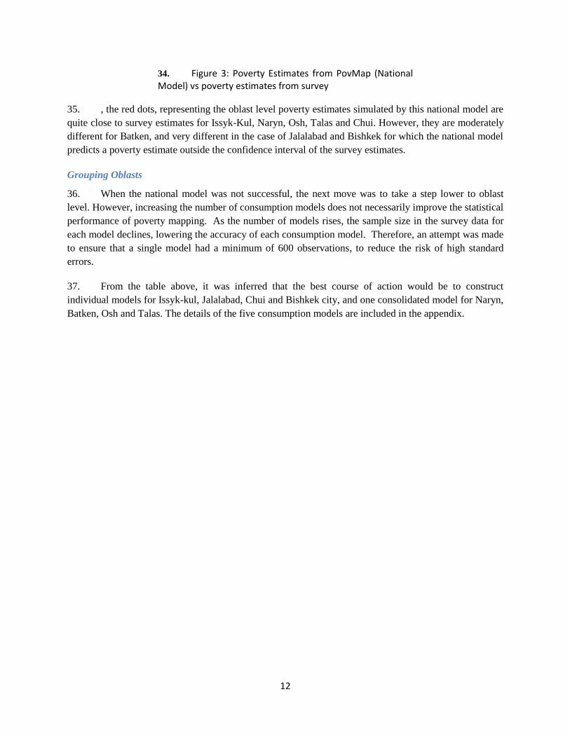
34. Figure 3: Poverty Estimates from PovMap (National Model) vs poverty estimates from survey

35. , the red dots, representing the oblast level poverty estimates simulated by this national model are

quite close to survey estimates for Issyk-Kul, Naryn, Osh, Talas and Chui. However, they are moderately

different for Batken, and very different in the case of Jalalabad and Bishkek for which the national model

predicts a poverty estimate outside the confidence interval of the survey estimates.

Grouping Oblasts

36. When the national model was not successful, the next move was to take a step lower to oblast

level. However, increasing the number of consumption models does not necessarily improve the statistical

performance of poverty mapping. As the number of models rises, the sample size in the survey data for

each model declines, lowering the accuracy of each consumption model. Therefore, an attempt was made

to ensure that a single model had a minimum of 600 observations, to reduce the risk of high standard

errors.

37. From the table above, it was inferred that the best course of action would be to construct

individual models for Issyk-kul, Jalalabad, Chui and Bishkek city, and one consolidated model for Naryn,

Batken, Osh and Talas. The details of the five consumption models are included in the appendix.

13

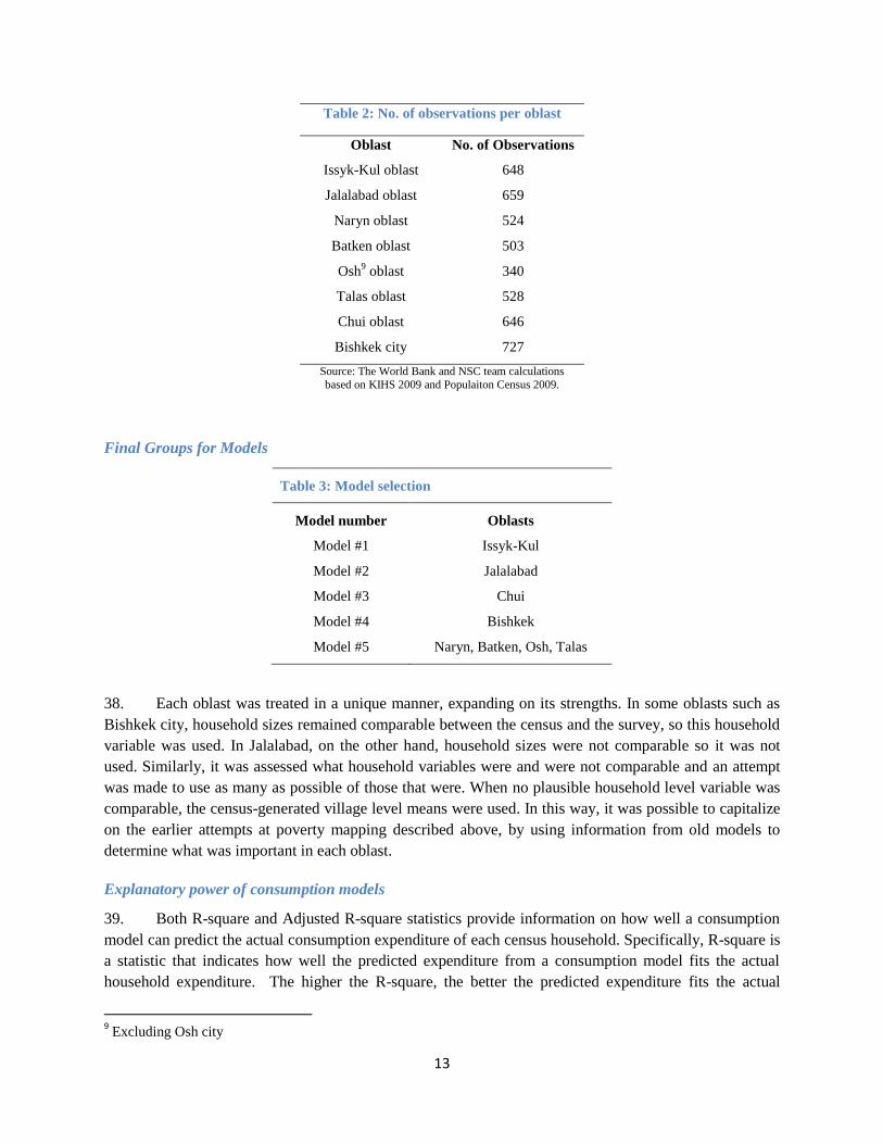
Table 2: No. of observations per oblast

Oblast No. of Observations

Issyk-Kul oblast 648

Jalalabad oblast 659

Naryn oblast 524

Batken oblast 503

Osh9 oblast 340

Talas oblast 528

Chui oblast 646

Bishkek city 727

Source: The World Bank and NSC team calculations

based on KIHS 2009 and Populaiton Census 2009.

Final Groups for Models

Table 3: Model selection

Model number Oblasts

Model #1 Issyk-Kul

Model #2 Jalalabad

Model #3 Chui

Model #4 Bishkek

Model #5 Naryn, Batken, Osh, Talas

38. Each oblast was treated in a unique manner, expanding on its strengths. In some oblasts such as

Bishkek city, household sizes remained comparable between the census and the survey, so this household

variable was used. In Jalalabad, on the other hand, household sizes were not comparable so it was not

used. Similarly, it was assessed what household variables were and were not comparable and an attempt

was made to use as many as possible of those that were. When no plausible household level variable was

comparable, the census-generated village level means were used. In this way, it was possible to capitalize

on the earlier attempts at poverty mapping described above, by using information from old models to

determine what was important in each oblast.

Explanatory power of consumption models

39. Both R-square and Adjusted R-square statistics provide information on how well a consumption

model can predict the actual consumption expenditure of each census household. Specifically, R-square is

a statistic that indicates how well the predicted expenditure from a consumption model fits the actual

household expenditure. The higher the R-square, the better the predicted expenditure fits the actual

9 Excluding Osh city

14

household expenditure. Adjusted R-square is a modification of R-square that adjusts for the number of

regressors in a model. R-square always increases when a new variable is added to a model, but adjusted

R-square increases only if the new variable improves the model more than would be expected by chance.

40. In the Kyrgyzstan Poverty Mapping Exercise, the adjusted R-square is generally quite high: 4 out

of 5 models record an adjusted R-square of over 43 percent and one model recorded an adjusted R-square

over 55 percent. For example, recent poverty mapping exercises in other countries, like Bangladesh and

India, some models have the adjusted R-squares less than 40 percent.

Table 4: Adjusted R2 of the different models

Model number Oblasts Adj. R2

Model #1 Issyk-Kul 56.77%

Model #2 Jalalabad 48.14%

Model #3 Chui 42.66%

Model #4 Bishkek 36.36%

Model #5 Naryn, Batken, Osh, Talas 47.48%

Source: The World Bank and NSC team calculations based on KIHS 2009 and Populaiton Census 2009.

Results of Poverty Mapping

41. The results from this grouping of models were successful and the poverty estimates obtained at

oblast level were not only well within survey confidence intervals but also had very low standard errors.

In addition, as stated above, the models had consistently high R2 s.

Table 5: Estimated poverty rates

Figure 4: Poverty estimates from PovMap (5 models) vs poverty estimates from survey

Oblast Poverty Rate Std. Error.

Issyk-Kul oblast 47% 0.00

Jalalabad oblast 33% 0.00

Naryn oblast 46% 0.02

Batken oblast 32% 0.02

Osh oblast 40% 0.01

Talas oblast 34% 0.02

Chui oblast 20% 0.01

Bishkek city 13% 0.01


Note: Oblast codes for this graph are as follows: 2-Issyk-Kul, 3-Jalalabad, 4-Naryn, 5-Batken, 6-Osh, 7-Talas, 8-Chui, 11-Bishkek

0.2

.4.6

.8

2 4 6 8 10 12Oblast

Conf. Int. (lower)/Conf. Int. (upper) Poverty Rate (survey)

Mod. Conf. Int. (lower)/Mod. Conf. Int. (upper) Poverty Rate (model)

15

IV. Maps

42. It is a natural perception that the incidence of poverty can vary markedly across localities within a

state or even within a smaller entity such as a rayon. The KIHS data, which is representative only at the

oblast level, does not allow for reliable estimates of poverty rates at the rayon level. As described in

section I, the ELL poverty mapping procedure combines census and survey data to generate estimates of

poverty incidence and inequality at levels of disaggregation such as the rayon. This section examines the

spatial patterns of estimated poverty and how they correlate with well-known determinants of poverty like

education, employment in agriculture, among others. In addition, this section provides a snapshot of poor

areas through poverty maps, including distributions of the poor population.

IV.1. Poverty Map

Figure 5: Poverty Map and Administrative Map of the Kyrgyz Republic


Note: For oblast boundaries, please refer to Figure 1. The above map shows the various rayons, and and the circles depict some towns

and cities that are often considered rayons themselves. The smaller circles depict selected populated areas, often rural areas.

43. Using the rayon-level poverty estimates simulated by the poverty mapping exercise, visual

representation of the incidence was created on maps of Kyrgyzstan10

, using shape-files. One of its most

striking features is to be able to visually depict spatial disparities that may not be obvious on examining

data.

44. In the poverty map above, the darker colors indicate higher incidence of poverty. The poorer

areas appear to be in the central parts of Kyrgyzstan. The border areas of Kyrgyzstan have a lower

incidence of poverty, probably due to their access and connectivity with surrounding countries –

particularly with affluent countries such as China to the east and south-east and Kazakhstan to the north.

10

By Brian Blankespoor (DECCT, The World Bank)

16

The circles in the map identify populated areas – most notably the capital city of Bishkek, which

predictably has a high population along with a low incidence of poverty.

45. Although a poverty headcount rate is no doubt among the more important poverty statistics, it can

be misleading at times for poverty alleviation purposes. For example, an area may exhibit a high poverty

rate, but might be sparsely populated, resulting in few poor people residing there. In contrast, a large city

might exhibit a low poverty rate, but represent a large concentration of the poor due to its high population

density. For this reason, a combination of information on which places have a high degree of poverty (a

map of poverty headcount rates) and where poor people live (a map of poor population) is useful for the

governments and the development partners to identify most in need areas and gauge the scale of resources

needed for the identified areas.

46. According to the World Development Report (WDR) of 2009, such maps not only help identify

the most in need areas, but also provide useful information on urban-rural linkages. The WDR 2009

argues that, if a country has many poor people living in poor areas (usually remote and rural areas), the

country, or at least the poor in the country, have not been able to fully exploit positive externalities from

urban agglomeration. In contrast, if many poor people are living in rich areas (usually large cities), the

country and even the poor have been able to enjoy the benefits of urban agglomeration.

Figure 6: Poverty Map and Poor Population Map of the Kyrgyz Republic

17


47. While the map of the distribution of the poor population above appears to be largely consistent

with the poverty map (first map in Figure 6), it must be noted that while a few districts (rayons) to the

east have poverty rates lower that 30%, they do have a sizeable share of the poor population. The opposite

may also be true, such as in the rayon Toguz-Torous, the poverty rate is greater than 75%, but the actual

poor population in absolute terms is moderate. When formulating policy, particularly for alleviating

poverty, it is important to note these nuances, as looking at a poverty map may suggest a very different

policy initiative than when both maps are studied in conjunction.

18

IV.2. Comparisons with maps of other socio-economic indicators

48. This section presents maps on the distribution of indicators that may provide some insight into

welfare outcomes and access to public services.

Figure 7: Market Accessibility Map and Poverty Map of the Kyrgyz Republic

Source: Market Accessibility from Blankespoor (2013) and the poverty map from the World Bank and NSC team estimations.

49. The market accessibility potential index is a measure of how far an area is from a group of select

major cities. In principle, the formula is a sum of population of the select major cities weighted by travel

time to reach there. Therefore, the index takes a larger score if surrounding cities are larger or travel time

to these cities is shorter. Geographic Information System software is used to find the shortest route and

estimate travel time based on road network data.

50. Predictably, areas near Bishkek and Osh city exhibit high market accessibility since both are large

cities. In contrast, central areas farthest from these cities have the lowest market accessibility. Some

19

mid-size cities (according to their being population centers) in the eastern areas (also due to Lake Issyk-

Kul) also have high market accessibility.

51. It is interesting to note that this is largely consistent with the poverty map, with the areas around

Bishkek and Osh having very low incidence of poverty. However, in terms of poor population, the

numbers are quite high even in these areas, particularly around Osh city. However, this is also owing to

the fact that, in general the population of these areas is quite high.

52. In the figure below, it is striking to note that the percentage of household members who are

employed is lower in a few of the less poorer regions of Kygyzstan, more notably the Bishkek area. This

could be because there may not be a need for too many household members to work as the working

members earn enough to support the whole household. In contrast to this scenario, is the low percentage

of employed household members in some poor areas such as a few central and southern districts. This

may represent a shortage of employment opportunities in the region.

Figure 8: Average percent of the household employed

20


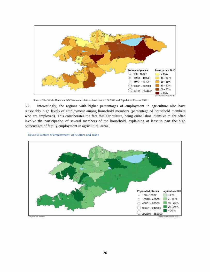
53. Interestingly, the regions with higher percentages of employment in agriculture also have

reasonably high levels of employment among household members (percentage of household members

who are employed). This corroborates the fact that agriculture, being quite labor intensive might often

involve the participation of several members of the household, explaining at least in part the high

percentages of family employment in agricultural areas.

Figure 9: Sectors of employment: Agriculture and Trade

21


54. The above figure depicts the percentage of the employed involved in trade confirms what can be

seen in the market accessibility map, namely that the two big trade centers in Kyrgyzstan are around

Bishkek and Osh city.

55. The figures below indicate that relatively poor regions in the center and western parts of the

country are coincident to regions where there is a high percentage of population whose highest

educational qualification is the completion of primary school. People with higher levels of education

(tertiary) appear to be concentrated around the capital area in the north, which is consistent with it being

the educational center. However, the same does not apply to Osh city where a quarter of the population

has at the most completed primary education.

22

Figure 10: Education (primary, secondary, tertiary)


V. Conclusion

56. This report summarizes the steps towards creating the latest poverty map of Kyrgyzstan and

overlays the poverty map with maps of other socio-economic indicators. Despite some methodological

challenges to constructing this map, we were able to produce it making the most of the data available to

us. To overcome this limitation, several village level aggregates of the available variables from the

Census were created. The more disaggregated the location variables, the more accurately household

expenditure can be estimated. Therefore, the success of this new Kyrgyzstan poverty mapping exercise

should rightly be attributed to the National Statistics Committee‟s effort to make the village codes

23

available for the analysis. Their effort made it possible to create these highly disaggregated means, in

place of the rayon level means that were available earlier.

57. Interesting observations come out after comparing the poverty map with the other maps. Poverty

incidence in border areas is in general low, with a few exceptions. This likely reflects the importance of

trade with neighboring countries. Reasonably high correlation between market accessibility and poverty

incidence further supports this hypothesis. A comparison between poverty incidence and poor population

reveals that big cities like Osh or Bishkek exhibit low incidence of poverty, but a high concentration of

poor population. This indicates that a low incidence of poverty does not necessarily imply that poverty

alleviation policies are not needed, and close attention must be paid to these pockets of poverty. The

correlation between education outcomes and poverty incidence is relatively limited.

58. A poverty map is a good monitoring instrument, but it becomes useful only if it is actively used

for policy making. Overlaying the poverty map with maps of other socio-economic indicators makes it

easy to identify what the key bottlenecks to poverty could be. Also, linking a poverty map and maps of

other outcome indicators with distribution of public expenditures would be highly useful to see how

outcomes and inputs are related. In fact, the Government of Kyrgyzstan and the World Bank have

recently completed the creation of a public expenditure database, which is organized by the World Bank‟s

software “BOOST”. This software enables one to see the linkage between distribution of the public

expenditure and outcomes like poverty, making such crucial information easily accessible to policy

makers.

24

References

Atamanov, A. and S. Sattar (2012). Regional disparities report. Kyrgyz Republic Programmatic Poverty

Assessment, mimeo.

Bigman, D. and U. Deichmann. (2000), „Spatial indicators of access and fairness for the location of public

facilities‟, in Geographical Targeting for Poverty Alleviation. Methodology and Applications, edited by

D. Bigman and H. Fofack, World Bank Regional and Sectoral Studies, Washington DC.

Library of Congress, Federal Research Division (2007). “Country Profile: Kyrgyzstan.”

Blankespoor, B. (2013). “Market Accessibility and Regional Maps: Kyrgyz Republic,” mimeo.

Elbers, C., J.O. Lanjouw, and P. Lanjouw (2002). “Micro-level estimation of welfare,” Policy Research

Working Paper Series no. 2911, The World Bank.

Elbers, C., J.O. Lanjouw, and P. Lanjouw (2003). “Micro-level Estimation of Poverty and Inequality,”

Econometrica, 71(1):355-364.

Ibraghimova, S. (2012). “Review of Sample Household and Labor Surveys in the Kyrgyz Republic,”

mimeo.

Jarvis, A., H.I. Reuter, A. Nelson, E. Guevara (2008). “Hole-filled SRTM for the globe Version 4”,

CGIAR-CSI SRTM 90m Database (http://srtm.csi.cgiar.org)

National Statistical Committee of the Kyrgyz Republic (2009). "Population and Housing Census of the

Kyrgyz Republic of 2009," Downloaded from http://cod.humanitarianresponse.info/country-

region/Kyrgyzstan, accessed 2012-08.

Tolipov, F. (2011). “Uzbekistan-Kyrgyzstan Relations after June 2010 Imply a Continued Lack of

Regionalism,” Central Asia Caucasus Institute Analyst.

Tarozzi, A. and A. Deaton (2009). “Using Census and Survey Data to Estimate Poverty and Inequality for

Small Areas,” Review of Economics and Statistics, 91(4), 773-792.

World Bank (2008), World Development Report 2009: Reshaping Economic Geography, the World

Bank, Washington, D.C.

Yefimova-Trilling, N. (2012). “Kyrgyzstan & Tajikistan: Disputed Border Heightens Risk of Conflict,”

Eurasianet.

http://www.cgiar-csi.org/2010/03/108/uot;http:/srtm.csi.cgiar.org

http://cod.humanitarianresponse.info/country-region/Kyrgyzstan

http://cod.humanitarianresponse.info/country-region/Kyrgyzstan

25

Appendix 1.

Model for Issyk-Kul R2=0.5817 adjR2=0.5677

Model variables

OLS Consumption

Model

GLS Consumption

Model

Variables Coeff. Std. Err. Coeff. Std. Err.

_intercept_

4.7298 0.2604 4.6614 0.203

AGE Age -0.0061 0.0013 -0.0074 0.0013

HHSIZE_MEAN_2 Village level average of household size squared -0.0145 0.0064 -0.0093 0.0039

HH_CHILD_RATIO Ratio of no. of children to total HH members -1.2133 0.0917 -1.2069 0.0897

HH_EDU_DUMMY1 Ratio of no. of HH members with higher prof. degree 0.3548 0.0685 0.3776 0.0734

HH_EDU_DUMMY3 Ratio of no. of HH members with secondary prof. degree 0.2964 0.0705 0.3686 0.0576

HH_EDU_DUMMY4 Ratio of no. of HH members with primary vocational degree 0.3787 0.0902 0.3841 0.0877

HH_EDU_DUMMY9_MEAN Village level mean of ratio of HH members who are illiterate 9.2419 3.2261 8.6219 2.8604

HH_IND_COMM_MEAN Village level mean of ratio of HH members employed in commerce 3.1398 0.9229 3.7405 0.6876

HH_WORKING_AGE_RATIO Ratio of no. of working age members to total HH members -0.3975 0.0669 -0.4181 0.0631

RAYON_2225_1 Rayon dummy -0.6482 0.1234 -0.6448 0.1155

SEX_1 Sex dummy 0.1501 0.0304 0.1412 0.0278

_HH_EDU_DUMMY2_MEAN$RAYON_2205#0 Interaction term of education level with Rayon dummy -19.0382 3.4875 -19.499 3.3543

_HH_EDU_DUMMY2_MEAN$RAYON_2210#0 Interaction term of education level with Rayon dummy 24.1624 2.8543 24.1552 2.6967






_HH_IND_COMM$RAYON_2210#0 Interaction term of occupation (commerce) with Rayon dummy 0.3902 0.1192 0.327 0.1095

_HH_IND_FIN$RAYON_2420#0 Interaction term of occupation (finance) with Rayon dummy 0.5023 0.1004 0.494 0.096

_HH_IND_MFG$RAYON_2210#0 Interaction term of occupation (manufacturing) with Rayon dummy 0.4187 0.1556 0.3585 0.1576

Model for Jalalabad R2=0.4948 adjR2=0.4814

Model variables OLS Consumption Model

GLS Consumption

Model


_intercept_

3.8074 0.061 3.8044 0.0562

HH_IND_DUM10 Ratio of HH members employed in unspecified activities 0.2387 0.1192 0.2687 0.1198

HH_IND_FIN Ratio of HH members employed in finance 0.2181 0.0668 0.1702 0.0675

HH_IND_TRADE_MEAN Village level mean of ratio of HH members employed in trade 1.6479 0.6232 1.6501 0.5669

HH_IND_TRANS Ratio of HH members employed in transport 0.2721 0.0661 0.281 0.0657

HH_OLD_RATIO Ratio of over 60 (age) members to total HH members 0.5387 0.0654 0.5778 0.0559

HH_WORKING_AGE_RATIO Ratio of no. of working age members to total HH members 0.5475 0.0573 0.5454 0.0554

RAYON_3215_1 Rayon dummy 0.2819 0.0333 0.2661 0.0315




26

SEX_1 Sex dummy 0.1093 0.0233 0.1145 0.0253

SEX_MEAN Village level mean of sex dummy -1.3787 0.2866 -1.3518 0.258

TOILET_MEAN Toilet dummy 0.5566 0.0783 0.5539 0.0707

_HH_EDU_DUMMY1$RAYON_3225#0 Interaction term of education level with Rayon dummy 0.5226 0.0638 0.5333 0.0597



_HH_EDU_DUMMY9$RAYON_3420#0 Interaction term of education level with Rayon dummy -0.3619 0.1435 -0.3307 0.1428

Model for Naryn, Batken, Osh and Talas

R2=0.4825 adjR2=0.4748


GLS Consumption

Model


_intercept_

5.3557 0.1455 5.5569 0.1671

DWELL_OWN_3 Type of Dwelling owned 0.1202 0.0412 0.0864 0.0379

HHSIZE HH size -0.3039 0.0173 -0.2999 0.0155

HHSIZE2 HH size squared 0.0163 0.0018 0.0163 0.0015

HH_EDU_DUMMY4_MEAN

Village level mean of ratio of HH members who have primary

vocational degree -1.9698 0.5132 -2.1148 0.6958

HH_IND_MFG_MEAN Village level mean of ratio of HH members employed in manufacturing -3.0806 1.0958 -3.283 1.1281





SEX_MEAN Village level mean of sex dummy -1.2629 0.2903 -1.475 0.326

_HHSIZE_MEAN$RAYON_4210#1 Interaction term of HH size village mean with Rayon dummy -0.0499 0.02 -0.0482 0.0231


_HHSIZE_MEAN$RAYON_4235#0 Interaction term of HH size village mean with Rayon dummy 0.0499 0.0083 0.0478 0.0132







_HH_IND_EGW_MEAN$RAYON_4210#1 Interaction term of occupation (elec, gas & water) with Rayon dummy 150.291 45.9702 153.1182 56.1497

_HH_IND_EGW_MEAN$RAYON_5236#1 Interaction term of occupation (elec, gas & water) with Rayon dummy -138.0274 30.4097 -145.8496 24.7981



_HH_IND_TRADE_MEAN$RAYON_4245#1 Interaction term of occupation (trade) with Rayon dummy 16.564 3.2646 19.6583 5.8034


_HH_IND_TRADE_MEAN$RAYON_6207#1 Interaction term of occupation (trade) with Rayon dummy -4.5712 0.8202 -4.4963 0.761


_HH_IND_TRADE_MEAN$RAYON_7232#1 Interaction term of occupation (trade) with Rayon dummy -42.0566 7.0623 -32.3349 8.6524

27

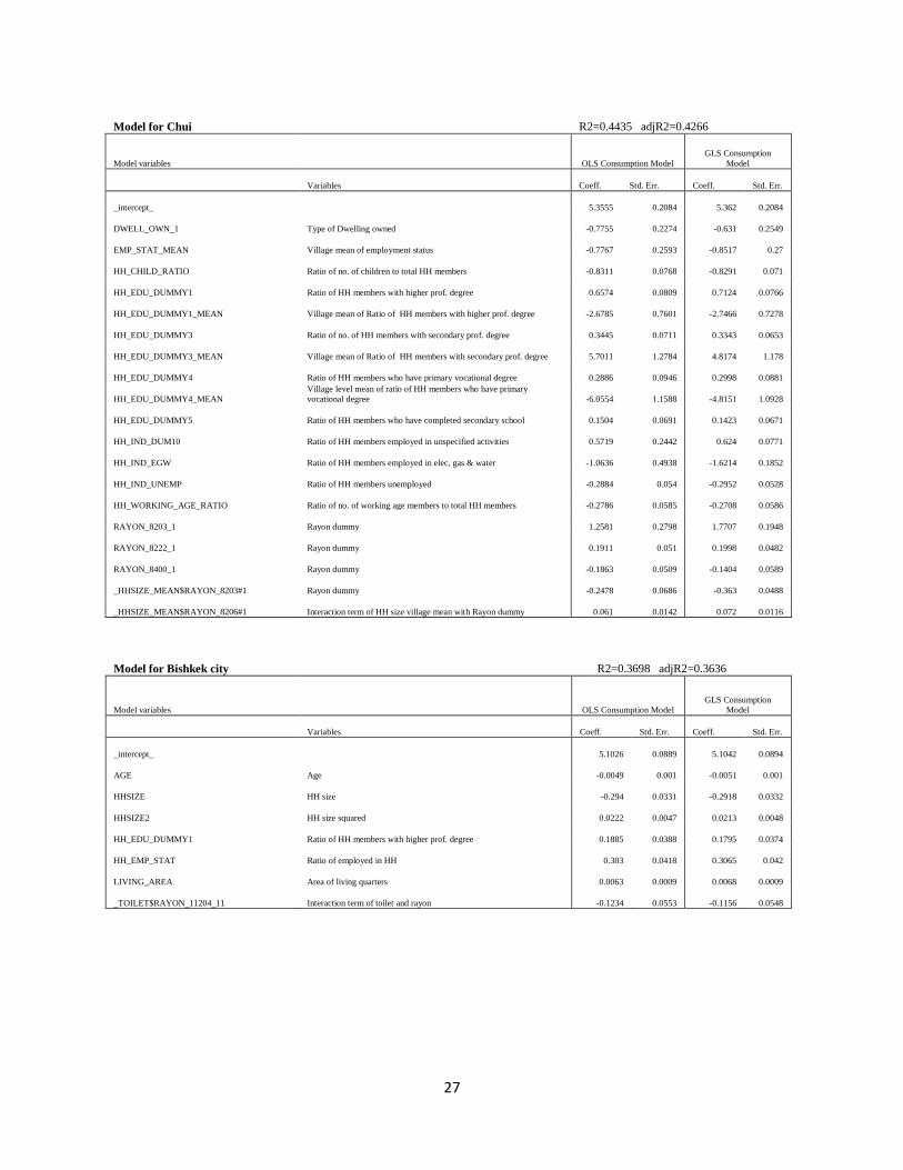
Model for Chui

R2=0.4435 adjR2=0.4266


GLS Consumption

Model


_intercept_

5.3555 0.2084 5.362 0.2084

DWELL_OWN_1 Type of Dwelling owned -0.7755 0.2274 -0.631 0.2549

EMP_STAT_MEAN Village mean of employment status -0.7767 0.2593 -0.8517 0.27

HH_CHILD_RATIO Ratio of no. of children to total HH members -0.8311 0.0768 -0.8291 0.071

HH_EDU_DUMMY1 Ratio of HH members with higher prof. degree 0.6574 0.0809 0.7124 0.0766

HH_EDU_DUMMY1_MEAN Village mean of Ratio of HH members with higher prof. degree -2.6785 0.7601 -2.7466 0.7278

HH_EDU_DUMMY3 Ratio of no. of HH members with secondary prof. degree 0.3445 0.0711 0.3343 0.0653

HH_EDU_DUMMY3_MEAN Village mean of Ratio of HH members with secondary prof. degree 5.7011 1.2784 4.8174 1.178

HH_EDU_DUMMY4 Ratio of HH members who have primary vocational degree 0.2886 0.0946 0.2998 0.0881

HH_EDU_DUMMY4_MEAN

Village level mean of ratio of HH members who have primary

vocational degree -6.0554 1.1588 -4.8151 1.0928

HH_EDU_DUMMY5 Ratio of HH members who have completed secondary school 0.1504 0.0691 0.1423 0.0671

HH_IND_DUM10 Ratio of HH members employed in unspecified activities 0.5719 0.2442 0.624 0.0771

HH_IND_EGW Ratio of HH members employed in elec, gas & water -1.0636 0.4938 -1.6214 0.1852

HH_IND_UNEMP Ratio of HH members unemployed -0.2884 0.054 -0.2952 0.0528

HH_WORKING_AGE_RATIO Ratio of no. of working age members to total HH members -0.2786 0.0585 -0.2708 0.0586




_HHSIZE_MEAN$RAYON_8203#1 Rayon dummy -0.2478 0.0686 -0.363 0.0488


Model for Bishkek city R2=0.3698 adjR2=0.3636


GLS Consumption

Model


_intercept_

5.1026 0.0889 5.1042 0.0894

AGE Age -0.0049 0.001 -0.0051 0.001

HHSIZE HH size -0.294 0.0331 -0.2918 0.0332

HHSIZE2 HH size squared 0.0222 0.0047 0.0213 0.0048

HH_EDU_DUMMY1 Ratio of HH members with higher prof. degree 0.1885 0.0388 0.1795 0.0374

HH_EMP_STAT Ratio of employed in HH 0.303 0.0418 0.3065 0.042

LIVING_AREA Area of living quarters 0.0063 0.0009 0.0068 0.0009

_TOILET$RAYON_11204_11 Interaction term of toilet and rayon -0.1234 0.0553 -0.1156 0.0548

28

Table. Poverty Rates and Standard Error per Rayon

Rayon Rayon name Population

Poverty

rate

Standard error of

poverty

41704210 Ak-Talaa 29650 0.383 0.0372

41704220 At-Bashy 49029 0.1764 0.025

41704230 Jumgal 40015 0.4636 0.0327

41704235 Kochkor 57519 0.6178 0.0265

41704245 Naryn 42785 0.7016 0.0243

41704400 Naryn town 33051 0.3495 0.063

41705214 Batken 68308 0.2254 0.0287

41705236 Leilek 99865 0.2422 0.0405

41705258 Kadamjai 152713 0.4638 0.0227

41705410 Batken town 18795 0.0945 0.0356

41705420 Sulukta 18333 0.1772 0.0449

41705430 Kyzyl-Kia 43089 0.2778 0.0802

41706207 Alai 59687 0.6206 0.0472

41706211 Aravan 97757 0.3209 0.0255

41706226 Kara-Suu 327038 0.423 0.0262

41706242 Nookat 233756 0.2831 0.0232

41706246 Kara-Kulja 85844 0.4382 0.0297

41706255 Uzgen 219523 0.469 0.0315

41706259 Chon-Alai 22241 0.2585 0.0273

41707215 Kara-Buura 57248 0.5887 0.0366

41707220 Bakai-Ata 41990 0.4295 0.031

41707225 Manas 32344 0.1806 0.0303

41707232 Talas 55297 0.0814 0.028

41707400 Talas town 30830 0.3545 0.0831

41702205 Aksui 60705 0.3141 0.0051

41702210 Jeti-Oguz 76727 0.8031 0.0084

41702215 Issyk-Kul 73003 0.3053 0.0048

41702220 Ton 47437 0.6332 0.014

41702225 Tup 55903 0.6951 0.01

41702410 Karakol 59828 0.1837 0.0071

41702420 Balykchi 41858 0.2876 0.0059

41703204 Ala-Buka 86547 0.3438 0.0061

41703207 Bazar-Korgon 138485 0.3715 0.006

41703211 Aksyi 112016 0.4964 0.006

41703215 Nooken 115364 0.0758 0.0058

41703220 Suzak 231232 0.3683 0.0056

41703223 Toguz-Toro 21853 0.7845 0.0082

41703225 Toktogul 85209 0.5321 0.0066

41703230 Chatkal 20888 0.162 0.0095

41703410 Jalal-Abad 84168 0.1509 0.0061

41703420 Tash-Kumyr 33651 0.0876 0.0147

29

41703430 Maili-Suu 19863 0.1585 0.0075

41703440 Kara-Kul 22164 0.0561 0.0053

41708203 Alamudun 140275 0.1508 0.0086

41708206 Issyk-Ata 128786 0.1102 0.0098

41708209 Jayil 89813 0.2275 0.0142

41708213 Kemin 41942 0.242 0.0126

41708217 Moscow 80799 0.3219 0.0111

41708219 Panfilov 41029 0.2196 0.0125

41708222 Sokuluk 151280 0.1529 0.0094

41708223 Chui 43959 0.2817 0.0101

41708400 Tokmok 51935 0.3463 0.0307

41711201 Leninsky 189128 0.1126 0.0067

41711202 Oktyabrsky 214786 0.117 0.0066

41711203 Pervomaysky 146427 0.1108 0.0067

41711204 Sverdlovsky 193976 0.1776 0.0075

30

Appendix 2. Sampling of the Kyrgyz Integrated Household Survey 2009 (Shamsiya Ibraghimova,

2012)

The 1999 Population Census was used as a sample frame of KIHS. The smallest territorial units available

in the computer database were the portfolios, which were compiled during the Census operation, of up to

400 persons in each. Based on the Census data, 13,067 portfolios have been compiled, which were

sufficiently homogenous in terms of the number of Census questionnaires. The available Census data

allowed using a two-stage sample design:

On the first stage, by using Census portfolios as primary sampling units, and the number of

households as a portfolio size, a certain number of portfolios was selected (primary sampling

units - PSU) through the haphazard procedure, with probability proportional to the portfolio

size.

On the second stage, by using household listings from the selected PSUs, a certain number of

households were randomly selected, with probability proportional to the household size.

Prior to the formulation of the sample for household survey across the country, measures have been taken

to determine the size of the sample and to identify the optimal method for households selection, i.e., the

design of the sample was developed in the initial phase of sample formulation. More detailed discussion

of sample design and formulation can be found in the report of the Consultant on Sampling, Mr. Juan

Muñoz (Annex А).

The first factor taken into account when designing the sample was the need to report survey data broken

into rural and urban areas by country regions. These 15 groups (seven oblasts including rural and urban

areas, and Bishkek city) became the main focal areas for integrated household budgets and labor force

survey estimates. Each of these areas were represented by a separate stratum, therefore, the initial task

was to distribute 5,000 households across 15 strata.

Due to the fact that the survey was planned to incorporate a section on labor force, there was also a need,

when distributing households among strata, to account for fluctuations of unemployment levels in each of

the strata, and unemployment homogeneity in each of the selected census portfolios.

Obviously, it was envisaged that the results of the survey will be used for comparative analysis between

oblasts, as well as for obtaining acceptable estimations both at the national and at the regional levels. It

was also considered in the sample design that the number of sampled households should be divisible by

11 (number of households per PSU), the number of PSUs should be a multiple of 6 (workload per 1

interviewer) and divisible by 12 to provide for a 12-percent rotation of the sample.

Upon consideration of various methods of sample composition, finally a sample distribution method was

selected with standard error smoothing.

31

Table: Sample distribution by regions

Oblast

Number of PSUs Number of households Standard error

urban rural total urban rural total urban rural total

Bishkek 72 0 72 792 0 792 2,4% 0% 2,4%

Issykkulskaya

oblast 36 24 60 396 264 660 4,0% 2,8% 2,3%

Jalalabadskaya

oblast 36 24 60 396 264 660 3,8% 2,1% 1,8%

Narynskaya oblast 24 24 48 264 264 528 4,5% 2,7% 2,4%

Batkenskaya

oblast 24 24 48 264 264 528 5,1% 2,4% 2,2%

Oshskaya oblast 36 24 60 396 264 660 3,7% 1,6% 1,5%

Talasskaya oblast 24 24 48 264 264 528 3,8% 2,3% 2,0%

Chuiskaya oblast 24 36 60 264 396 660 4,4% 2,7% 2,3%

Country Total 276 180 456 3 036 1 980 5 016 1,5% 0,9% 0,8%

Whereas such sample distribution increases standard error by 0.1% for the country overall, the estimate

deviations by strata with such sample distribution will be smoothed out significantly.

The following conclusions may be drawn from the consideration of the selected portfolios profiles, which

impact on the design of the sample:

All strata are sufficiently large, and, therefore, the accuracy of the sample will be determined by

the absolute size of the sample.

Unemployment is much higher in urban areas than in rural areas. Thus, although two thirds of

the country population are rural dwellers, urban areas require more surveying.

Intra-portfolio unemployment rate correlation suggests that out from the given number of

households, the maximum possible number of PSUs should be visited with a small number of

households in each.

When determining the number of PSUs, it should be taken into account that the PSU number

must be a multiple of 6 to regulate workload per interviewer, and also be a multiple of 12 to

ensure the 12-percent rotation of the sample.

In this manner, on the first sampling stage portfolios have been randomly selected in each of 16 strata,

with probability proportional to the number of households in portfolios. In total, 456 portfolios have been

selected for the country.

On the second stage, 11 households have been randomly selected in each portfolio, with probability

proportional to the size of the households. Then the codes have been identified of the households included

in the sample, and the listings prepared with indication of PSU locations and households addresses.

32

Considering the fact that household selection probability varies between strata, for the purpose of survey

data spreading over the country as a whole, spreading coefficients need to be calculated by strata.

Spreading coefficients are obtained from the following formula:

i

i

in

NW ,

where iW - is a household's weight in stratum i;

iN - number of households in stratum i;

in - number of households in stratum i included in the sample.

In the course of sample selection, problems have been encountered, which are related with

incompleteness of the address part of the households' entries. The work carried out on preparation of the

household lists for each PSU detected that there are populated areas in the Kyrgyz Republic, where street

names and house numbers are not available. Where such areas were included in the sample, additional

work was carried out on refining household lists by using Village Councils' (at present Village Districts)

data on availability of the household economic record books ('economic books') and accounts therein.

These data were collected for each population center in rural areas in February and April 2002. For each

population center, a certain number of economic books were selected, equal to the number of census

portfolios selected for such population center. Then, depending on the number of personal accounts in the

selected book, the sampling interval was calculated (number of accounts / 11), and then a systematic

selection of personal accounts was made starting from the randomly selected beginning (within the

sampling interval) and using the sampling interval so calculated. In this manner, the rule of random

household selection was observed, preventing potentially subjective approach to the selection of

households in the localities.

Under the new sample design, the number of primary sample units was increased almost 3.8 times (the

old sample is marked with asterisks). However, attention should be drawn to the fact that the size of the

sample increased only 1.7 times. Sample distribution may be clearly seen on the map, where PSUs

included in the new sample are marked with grey circles. It also may be seen that on some occasions the

same PSUs were included in the new sample, which have been used in the old sample. Such cases are

marked with starlets inside the gray circles.

33

Figure: PSU distribution across regions of the country.

Source: NSC publication

Thus, the sample size was determined of 5,016 households. To prevent biased sample selection, any

substitution of addresses is inadmissible on all subsequent stages of the work.

Household survey in the Kyrgyz Republic is conducted on the continuous basis, i.e., quarterly.

Households included in the sample are surveyed in accordance with a certain timetable, and thereafter

new households are selected as a substitution for them.

As a matter of practice, a number of HHs drops out from the survey during the year for various reasons.

Due to this, the need arises to substitute the dropouts for new ones for the next year. In order to retain the

distribution of the number of the surveyed HHs by months, it is recommended to conduct surveys of the

new HHs during those specific months, when the previous HHs have been dropped.

Poverty Mapping in the Kyrgyz Republic1 - The World...

Documents

Transcript of Poverty Mapping in the Kyrgyz Republic1 - The World...