Poverty, growth, and environment in Brazil: spatial insights for...
111
Poverty, growth, and environment in Brazil: spatial insights for policymaking April 2006 Environmental and Socially Sustainable Development Latin America and the Caribbean Region Note to the reader: The graphics in this report are intended to be viewed or printed in color.
-
Upload
hoangquynh -
Category
Documents
-
view
220 -
download
3
Transcript of Poverty, growth, and environment in Brazil: spatial insights for...

Poverty, growth, and environment in Brazil:
spatial insights for policymaking
April 2006
Environmental and Socially Sustainable Development Latin America and the Caribbean Region
Note to the reader: The graphics in this report are intended to be viewed or printed in color.

Spatial insights for policy page ii
Acknowledgments
This report is an output of the “Brazil Spatial Approach” study, managed by Kenneth Chomitz under the supervision of L. Gabriel Azevedo. It was drafted by Chomitz, drawing on contributions from a number of sources. The labor market analyses of section 2 draws on, and in some cases quotes, joint work with colleagues in the Urban and Regional Directorate of IPEA, especially Daniel da Mata, Alexandre Ywata de Carvalho, and João Carlos Magalhaes. The review of spatial policies in section 1 including the analysis of water system costs is based on a draft by Edinaldo Tebaldi. Timothy Thomas contributed to the analyses of the spatial distribution of RPAP and PRONAF funds. Some of the Northeastern and Ceara GIS data used in section 3 was compiled by Sonia Barreto Perdigão de Oliveira and Mauro Santos de Melo of FUNCEME under the direction of its president, Francisco de Assis de Souza Filho. Marcos Holanda and Claudio Andre Gondim Nogueira of IPECE collaborated in the weather analysis. The Amazonian analysis of section 4 draws on work by Sheila Wertz-Kanounnikoff and was supported in part by a German Consultant Trust Fund. Other GIS analysis was undertaken by Jonny Andersson and Piet Buys. The discussion in section 4 draws heavily on work sponsored by the Global Overlay program, the Research Support Board sponsored Economic Instruments for Conservation Project, undertaken in collaboration with IESB, Conservation International and the University of California, Santa Barbara.
An earlier, condensed version of some of this material was presented at the Fórum Nacional in 2005 and was published as Kenneth M. Chomitz, “Políticas de desenvolvimento para um espaço heterogêneo”,. in O Desafio da China e da Índia: A Resposta do Brasil, João Paulo dos Reis Velloso (coord.), Editora José Olympio, Rio de Janeiro, RJ, 2005.
We are grateful to Alex Araujo, Francisco de Assis de Souza Filho, Marco Holanda, and Marcelo Piancastelli for valuable discussions. Helpful comments were provided by Tulio Barbosa, Edward Bresnyan, Luis Coirolo, Uwe Deichmann, Somik Lall and by peer reviewers Francisco Ferreira, Antônio Magalhaes, and Dorte Verner.
Disclaimer
This report is a product of the staff of the International Bank for Reconstruction and Development/ The World Bank. The findings, interpretations, and conclusions expressed in this paper do not necessarily reflect the views of the Executive Directors of The World Bank or the governments they represent. The World Bank does not guarantee the accuracy of the data included in this work. The boundaries, colors, denominations, and other information shown on any map in this work do not imply any judgment on the part of The World Bank concerning the legal status of any territory or the endorsement or acceptance of such boundaries.
The material in this publication is copyrighted. Copying and/or transmitting portions or all of this work without permission may be a violation of applicable law. The International Bank for Reconstruction and Development/ The World Bank encourages dissemination of its work and will normally grant permission to reproduce portions of the work promptly.
For permission to photocopy or reprint any part of this work, please send a request with complete information to the Copyright Clearance Center, Inc., 222 Rosewood Drive, Danvers, MA 01923, USA, telephone 978-750-8400, fax 978-750-4470, http://www.copyright.com/.

Spatial insights for policy page iii
All other queries on rights and licenses, including subsidiary rights, should be addressed to the Office of the Publisher, The World Bank, 1818 H Street NW, Washington, DC 20433, USA, fax 202-522-2422, e-mail [email protected].

Spatial insights for policy page iv
Abbreviations
CCM Chomitz, Carvalho, and da Mata (in prep.)
CMCM Chomitz, da Mata, Carvalho, Magalhaes (2005)
FNE Constitutional fund for the Northeast
HDI Human Development Index
IBGE Instituto Brasileiro de Geografia e Estatística
IPEA Instituto de Pesquisa Econômica Aplicada
IUS-WwC Brazil: Inputs for an Urban Strategy - Working with Cities
MCA Minimum Comparable Area (of municipios)
PRONAF Programa Nacional de Fortalicemento da Agricultura Familiar
RED: Brazil: Regional Economic Development – (Some) Lessons from Experience
RPAP Rural poverty alleviation project
ZFM Zona Franca de Manaus

Spatial insights for policy page v
Executive Summary
This report examines the implications of spatial heterogeneity – the uneven distribution of poverty, growth, and environmental assets – for policy. Its goal is to inform a wide set of policies that are either explicitly spatially targeted or may have unanticipated spatial implications. These include:
• Poverty alleviation policies targeted on poor municipios • Demand-driven poverty alleviation policies • ‘Territorial development’ policies aimed at stimulating growth in a multi-
municipio region • Growth policies targeted on semi-arid regions • Policies to protect environmental assets
The report does not assess particular policies in detail; it complements two contemporaneous Bank reports that look at urban policies and at regional development policies such as fiscal incentives and subsidized loans.. Rather, it focuses on clarifying some of the fundamental assumptions and underpinnings of spatially oriented development policies, addressing six questions organized in three sections:
Spatial inequality and policy targeting • Are policies targeted at poor municipios effective in reaching poor people? • Do demand-driven policies favor poor people?
Policy lessons of spatial heterogeneity in poverty and growth • What explains divergent labor market experiences in rural areas? • Are poverty and economic stagnation in the Northeast closely tied to
agroclimatic conditions? Reconciling forest conservation with poverty reduction and agricultural development
• Is poverty a major determinant of Amazonian deforestation? • Is there a steep trade-off between forest protection and agricultural output?
The report advances knowledge in each of these areas, but unresolved issues remain for debate and research.
Policies targeted at poor municipios may be inefficient in reaching poor people
Concerns about spatial inequality have been heavily shaped by a focus on poverty rates rather than poverty densities. These alternative definitions of ‘poor areas’ yield radically different poverty maps. (See below; red=high rates or densities.) Municipios with the lowest poverty rates (equivalently, low human development index or HDI) tend to have high poverty densities, so that many poor people live in high HDI municipios. High poverty rate (or low HDI) municipios vary greatly in poverty density. Among municipios with poverty rates in the 60% to 80% range, poverty densities vary from barely 1 person per km2 to over 150.
.

Spatial insights for policy page vi
Proportion of people who are indigent, 2000 Indigent people/km2, 2000
Low-poverty-density municipios face another challenge: high unit costs of service and infrastructure provision. Grid-connected electricity and rural roads are examples of infrastructure with increasing returns to density. For these reasons, programs – of which there are many – that direct priority funding to low HDI municipios merit reconsideration with regard to their goals. If the goal is to reduce aggregate poverty, then this approach may be inefficient. It assigns lower priority to more numerous groups of poor people who can potentially be served at lower unit costs.
On the other hand, some interventions, such as transfers, may be more efficacious in targeting resources on the poor when poverty rates are high, because this minimizes leakage to nonpoor, or costs of screening out the nonpoor. These considerations suggest that a typology based on high vs. low poverty density and high vs. low poverty rate can be a useful starting point for considering local development policies. Probably the greatest challenge is faced by areas with high poverty rates and low poverty densities. Areas with these conditions might want to explore trade-offs among different lines of intervention. For instance, investments in telecommunications and education might have higher payoffs than feeder roads. Direct transfers provide a benchmark against which to assess productive investments for these difficult areas.
Demand-driven programs can have unexpected spatial impacts
Demand-driven programs such as PRONAF, the FNE, and community-driven development projects combine eligibility rules based on location with demand-responsive allocation. In principle, demand-driven programs solve problems associated with other forms of spatial allocation of resources. Technocratic, top-down planning (e.g., picking spatial winners) risks the appearance or actuality of bias. Formula-based allocation of funds is transparent and impartial, but it could be inefficient if it fails to recognize that investments may have differential impacts among places due to differences in local capacity. Demand-based programs appear to combine transparency with efficiency, by filtering eligibility and favoring capable participants.
However, the spatial outcomes of demand-driven programs may be unexpected, reflecting behavior of both demanders and suppliers. Geographic analysis can be used to detect and diagnose factors that influence allocation. An analysis of the Bahia rural poverty alleviation

Spatial insights for policy page vii
project shows that, expenditures per poor person are much higher in very low-population municipios in low rainfall areas. Further analysis is necessary to determine the reason for this concentration, and to assess whether program expenditures have higher impacts in these areas. PRONAF rural credits, aimed at family farmers, also exhibit marked geographical concentrations at the national level. The South received about half of the R$6 billion disbursements in 2004-5, but has only 18% of rural workers. Further analysis is necessary to determine whether this pattern of concentration reflects higher rates of landholdings, higher educational levels, or perceived lower risk levels for farms in favorable agroclimatic areas. Within the Northeast, spatial patterns of allocation of PRONAF credits were largely unrelated to poverty or literacy rates. However, policies favoring the semi-arid seem to have been effective. Other things equal, location in the semi-arid was associated with an increment of 7.6 Group B or C contracts (those aimed at the poorest farmers) per 100 rural residents; the overall mean incidence was 6.2.
Dynamic metropolitan areas absorbed labor while also increasing mean labor earnings
“Dynamic metropolitan areas” are large urban agglomerations that exhibited both growth in mean labor earnings over 1991-2000 and employment growth more rapid than mean national population growth. These areas had 32% of Brazilian employment in 1991, but absorbed 53% of the country’s net increase in employment, with immigration apparently playing a large role. The success of these areas in boosting earnings is remarkable in view of this report’s finding that, other things equal, wages decline elastically in response to an increase in labor supply. This suggests that it is possible for large cities to boost demand rapidly enough to accommodate newcomers. This parallels the finding of a companion report that metropolitan areas with rapid growth in formal housing can grow in total population while decreasing their slum population.
Education, transfers, and spillovers boost earnings growth in nonmetropolitan areas
Over the 1990s there were starkly divergent economic trends between the Northeast and the rest of the country – but also, considerable within-region heterogeneity. The figure left depicts labor market dynamics for non-metropolitan areas. Areas in red experienced a drop in average earnings per worker between 1991 and 2000. The areas shown in dark red experienced both a decline in earnings and slower than average growth in employment, suggestive of a local economic decline. The pink areas are stagnant: in these areas, employment grew rapidly, but earnings fell. Areas in light blue experienced growth in both earnings per worker and in employment.
Analyses of these patterns at both national and Northeastern levels (undertaken in collaboration with IPEA) found that increases in average earnings were strongly related to the initial level of education of the workforce. One year of additional earnings accounted for an additional 6 to 8 percentage point increase in the nine year growth rate of earnings/

Spatial insights for policy page viii
Differences in educational attainment account for much of the difference in earnings growth between the southern and northern parts of the country. This dynamic effect is distinct from, and in addition to, the more well-known relationship between education levels and wage levels. Although it is not possible to conclude that the relationship is causal (there could be complex feedbacks between local social capital and mean education, for instance), these finding direct additional weight towards educational investments as a means of helping lagging regions, either by boosting local earnings or facilitating outmigration.
The analyses also found evidence that income growth in urban areas could enhance both earnings and employment growth in neighboring rural areas. This suggests that if secondary city growth could be stimulated, as many hope, there could be significant spillovers to local areas. Though not a subject of this report, however, there is little solid guidance on the efficacy of ‘territorial development’ and ‘cluster’ approaches. A cautious approach would insist that any attempt at promoting secondary city growth have a firm economic rationale – for instance, addressing coordination failures in providing training, infrastructure, or marketing support for local industries, or investing in complements to local natural resources.
Increases in transfers had a powerful effect on boosting average earnings – perhaps because low-wage pensioners were induced to withdraw from the labor market, but perhaps also as a result of low multiplier effects as the pensioners increased their demand for local services.
Climate may not be the most important constraint on northeastern growth and poverty alleviation.
Cross-sectional analysis found that education, rather than location in the semi-arid, was the main correlate of poverty and child mortality in the Northeast. (See graphs, which distinguish ‘more difficult’ and ‘less difficult’ regions within the semi-arid.). The connection may be only partly causal; low educational attainment may itself reflect unfavorable social conditions. The strength of the association suggests however that, in looking to relax local constraints, we look more closely at human and social capital than at agroclimate --- at the implications of addressing functional illiteracy, for instance, rather than at remediating soils or lack of water.
Indigency and education Child mortality and education

Spatial insights for policy page ix
There is also a strong association between increases in household transfer payments (presumably mostly rural pensions) and decreased poverty rates.
However, as one would expect, the semi-arid does have some detectable influences on welfare. Location in the semi-arid regions is associated with lower labor earnings, other things equal. And this report presents evidence that economic sensitivity to climatic fluctuations is most serious in the most agroclimatically constrained part of the semi-arid. In the caatinga of Ceara, rainfall 20% below average is associated with a 5% reduction in municipal agricultural GDP; outside the caatinga there is no statistically significant relationship. This finding focuses attention on interventions, such as weather insurance, related specifically to these constraints and benefiting the rural dwellers who are most exposed to these conditions, rather than more diffuse preferences for the entire semi-arid. The report used census-tract level data to quantify the number of rural people living in the most difficult part of the semi-arid (roughly equivalent to the sertão) and estimated this population at about 4.0 million in 2000, a reduction of about 10% from 1991.
Poverty is not a major driver of Amazônian deforestation
Amazonia has poor people and rapid deforestation, but the link between the two is relatively weak. (see below). There are poor people undertaking deforestation in Amazonia, but they
account for a relatively small portion of total deforestation, and deforestation is not generally the cause of their poverty. While this may be relatively well known among specialists, it is not fully appreciated by the wider public, and this report provides new supporting evidence. Over the period 2000-2003, incremental annual forest clearings of less than 20 hectares

Spatial insights for policy page x
(which presumably encompass most small-farmer activity) accounted for only 19% of total deforestation. Clearings of over 200 hectares, which presumably reflect the actions of very large, well-financed actors, accounted for 39% of deforestation. Analysis shows also that deforestation rates are very closely related to the farmgate price of beef, suggesting a strong market rather than subsistence orientation of most deforestation. Distinct policy approaches are needed to address the problems of deforestation and rural poverty alleviation.
Economic instruments could sharply reduce trade-offs between forest conservation and agricultural development
In the Atlantic Forest and cerrado areas, agriculture vies for land with threatened ecosystems featuring very high levels of species endemism. Conservation policies are made more difficult by the need to conserve large contiguous forest areas in order to maintain ecological processes (e.g. the survival of viable populations of ‘charismatic’ primate species.). However, empirical and simulation studies suggest that the trade-offs may be less steep than imagined. A study in the Atlantic Forest of Bahia (undertaken in collaboration with IESB and Conservation International) found that land values were on average low, and were strikingly lower under forest cover. A related study simulated the impact of an auction-based system for environmental services, similar to those used in the US and Australia. It found that a R$80 million budget would elicit lands for reserves that would encompass twelve large distinct contiguous areas that each satisfied a ‘viability’ criterion, representing five of the eight sub-ecosystem types of the region.
Another set of studies looked at the impact of allowing trade in legal forest reserve. Many landholders are out of compliance with legal reserve regulations. Compliance under current inflexible rules would require these landowners to tear up productive fields and attempt to replace them with native vegetation. On the other hand, current practice would also allow conversion of forest to low-value pasture in areas that still have significant forest cover. Legal reserve trading offers, in theory, a superior outcome on both economic and environmental grounds, by letting the forest-poor landholder satisfy legal reserve obligations by purchasing services from the forest-rich landholder. A study that simulated a hypothetical such trading system for Minas Gerais found that it would reduce landholders’ compliance costs by about two thirds, compared to an inflexible, command and control system. Moreover, it would boost the proportion of legal reserve which is ‘high quality’ forest from 60% to 90%, and increase the protection designated as the highest priority for biodiversity conservation.
Directions for follow-on research.
The report highlights a number of specific areas for follow-up research and analysis.
o Invest in more monitoring and evaluation of demand-driven programs and ‘territorial devleopment’ initiatives. A number of large and expensive programs, such as the Constitutional Funds, community-driven development projects, PRONAF, are based on unexamined assumptions and do not mount monitoring and evaluation efforts proportional to the resources involved. Similarly, there is a great need to systematically evaluate the experience with territorial development and cluster approaches

Spatial insights for policy page xi
o Invest in a new Agricultural Census, and other spatial information. To assess program and policy impacts accurately, it is important to have detailed spatial information about ambient economic, social, and environmental conditions. While IBGE and INPE have made great strides in assembling and disseminating geographical information, there is need for further data integration and gap filling. An up-to-date Agricultural Census is urgently needed.
o Examine the economies of small rural towns, especially in the Northeast. Outside the metropolitan areas, mean incomes (and education) are very strongly related to the ‘urban’ proportion of the population. Here, ‘urban’ refers to small towns, with populations of a few thousand. More research is required in order to understand the policy significance of this correlation. What drives these micro-economies? Is it possible to stimulate their growth?
o Assess options for and impacts of service and infrastructure delivery in remote and/or low population density areas. Analysis and synthesis is needed on the costs and benefits of alternative technologies for delivering various services to these areas.
o Assess prospects for weather insurance as part of an overall water management system. Weather-based index insurance could help state and federal governments to better manage funding of disaster relief, and help farmers and firms better to manage year-to-year variation in productivity. Further studies are needed to understand the scope, mechanisms, and potential impacts of offering weather insurance.
o Critically examine the hypothesis that secondary city development reduces social and environmental externalities in large cities. Stimulating secondary cities is often justified on the grounds that it reduces the burden of migration-driven growth of the largest cities. This widely-accepted rationale, however rests on a whole chain of poorly-examined assumptions:
o Reliable, cost-effective policy interventions exist for stimulating secondary city growth
o More rapid growth of secondary cities will divert rural migrants away from primary cities
o Reduced immigration to primary cities will significantly reduce their population growth rates
o Reduced population growth rate of primary cities will lead to a reduction in social and environmental burdens (such as crime and pollution) and to better economic outcomes.
o The social benefits from reduced social and environmental burdens outweigh the losses in economic productivity associated with a shift in production from larger to smaller cities (which offer fewer scale economies).

Spatial insights for policy page xii
o It is cheaper to reduce those social and environmental burdens indirectly (by diverting migrants) than directly (e.g. by providing housing, police, and sanitation in the primary cities).
All of these propositions are in need of careful scrutiny; together they define a research agenda with important implications for the way that regional development is viewed.
.

Spatial insights for policy page xiii
CONTENTS 1. CONTEXT ...........................................................................................................................................1
INTRODUCTION AND OVERVIEW: THE CHALLENGE OF SPATIAL DEVELOPMENT ...........................................1 RATIONALES FOR SPATIAL POLICY ..............................................................................................................3
Poverty reduction in ‘poverty traps’......................................................................................................4 Spatial inequality reduction...................................................................................................................4 Unlocking growth potential ...................................................................................................................4 Reducing migration to large cities?.......................................................................................................5 Allocating land between agricultural production and forest conservation ...........................................5
SPATIAL DEVELOPMENT MECHANISMS IN PRACTICE....................................................................................5 Fiscal incentives and subsidies for lagging regions ..............................................................................6 Fomenting spatial winners: Territorial Development, Growth Pole, and Cluster Approaches ............7 Targeting poor municipios ....................................................................................................................8 Demand driven programs with spatial criteria......................................................................................9
2. ISSUES IN SPATIAL TARGETING...............................................................................................10
ARE POLICIES TARGETED AT POOR MUNICIPIOS EFFECTIVE IN REACHING POOR PEOPLE?...........................10 Poverty density differs from poverty rates ...........................................................................................10 Economies of scale and density in infrastructure and service provision .............................................16 A normative model of spatial allocation of expenditure ......................................................................23
DO DEMAND-DRIVEN PROGRAMS REACH POOR PEOPLE? ...........................................................................27 Example 1: The Bahia Rural Poverty Alleviation Project ...................................................................27 Example 2: Spatial allocation of PRONAF rural credits ....................................................................34
3. UNDERSTANDING SPATIAL DIFFERENCES IN ECONOMIC PERFORMANCE .............38
WHAT ACCOUNTS FOR DIFFERENTIAL LABOR MARKET PERFORMANCE BETWEEN MUNICIPIOS? ................38 TO WHAT EXTENT DO POOR AGROCLIMATIC CONDITIONS CONSTRAIN NORTHEASTERN GROWTH?.............45
Agroclimate and investments ...............................................................................................................45 How many people live in agro-climatically constrained areas in the Northeast? ...............................46 Geographic and policy determinants of labor market changes in the Northeast ................................53 Economic vulnerability to weather shocks ..........................................................................................54
SUMMARY AND IMPLICATIONS ..................................................................................................................57
4. FOREST CONSERVATION, POVERTY, AND AGRICULTURAL DEVELOPMENT ..........60
ENVIRONMENTAL ASSETS..........................................................................................................................60 DOES POVERTY DRIVE AMAZÔNIAN DEFORESTATION?..............................................................................61 IS THERE A STEEP TRADEOFF BETWEEN FOREST CONSERVATION AND AGRICULTURAL OUTPUT? ...............71
5. CONCLUSIONS................................................................................................................................76
PROPOSITIONS FOR FURTHER DISCUSSION .................................................................................................76 Thoughtfully articulate concerns about spatial inequality and goals for regional development; recognize the shortcomings of municipios as spatial planning units...................................................76 Experiment with territorial development approaches only where there are compelling rationales of comparative advantage and coordination. ..........................................................................................77 Relate growth and development interventions to poverty rate and poverty density.............................77 Tailor interventions in the semi-arid to the distinctive problems of the semi-arid ..............................78 Examine education and its correlates as a long-term instrument for reducing spatial inequalities....78 Frame rules for demand-driven programs carefully; monitor and evaluate performance..................78 Don’t assume that poverty alleviation and environmental protection are synonymous ......................79
DIRECTIONS FOR FUTURE RESEARCH, MONITORING AND EVALUATION, AND INFORMATION......................79 Invest in more monitoring and evaluation of demand-driven programs..............................................79 Assess the performance of territorial development and clustering initiatives .....................................79 Invest in the Agricultural Census, and other spatial information........................................................79 Examine the economies of small rural towns, especially in the Northeast ..........................................80

Spatial insights for policy page xiv
Assess options for and impacts of service and infrastructure delivery in remote and/or low population density areas. .......................................................................................................................................80 Assess prospects for weather insurance as part of an overall water management system. .................80 Assess alternative options for implementing legal reserve trading or other economic instruments for conservation.........................................................................................................................................80 Critically examine the hypothesis that secondary city development reduces social and environmental externalities in large cities...................................................................................................................81
Figures
Figure 1 Contrasting views of poverty and environment .............................................................. 2
Figure 2 Indigency rates, 2000......................................................................................................... 12
Figure 3 Indigency densities, 2000 .................................................................................................. 12
Figure 4 Cumulative poverty distribution by HDI, Northeast 2000.......................................... 13
Figure 5 Poverty densities vs. HDI, Northeast, 2000 .................................................................. 14
Figure 6 Extreme poverty density vs. rate, Northeast municipios ............................................. 14
Figure 7 Illiteracy density vs. rate, Northeast municipios........................................................... 15
Figure 8 Density vs. rate of nonenrolled children, Northeast municipios ................................ 16
Figure 9 Unit costs of electric grid connection ............................................................................. 17
Figure 10 Water supply costs and population density, Northeast, 2002 ................................... 19
Figure 11 Water supply costs and municipio size, Brazilian Northeast, 2002.......................... 19
Figure 12 Amazonas: rural proportion without improved water source................................... 20
Figure 13 Amazonas: rural density of population without improved water source ............... 21
Figure 14 Number of people without improved waters in urban and rural settlements ....... 22
Figure 15 Map of Bahia RPAP expenditure/population............................................................. 29
Figure 16 RPAP expenditure by municipio size and rainfalll ..................................................... 32
Figure 17 Incidence of PRONAF credits (group B and C) in the Northeast .......................... 36
Figure 18 Labor dynamics 1991-2000 ............................................................................................ 40
Figure 19 Education and earnings growth, Brazil......................................................................... 43
Figure 20 Northeast: Semi-arid areas, soils, rivers and urban settlements ................................ 47

Spatial insights for policy page xv
Figure 21 Rural population declined in the semi-arid between 1991 and 2000 ....................... 48
Figure 22 Population in "Extremely High Priority" areas for Caatinga biodiversity............... 49
Figure 23 Poverty is strongly inversely related to education....................................................... 50
Figure 24 Poverty is strongly inversely correlated with urban proportion................................ 51
Figure 25 Earnings/worker are strongly associated with education .......................................... 51
Figure 26 Child mortality declines with education ....................................................................... 52
Figure 27 Increased transfers are associated with decreased indigency..................................... 53
Figure 28 Ceará: caatinga and population density......................................................................... 56
Figure 29 Impact of weather shocks on agriculture in the Ceará caatinga................................ 56
Figure 30 Map of Amazonian deforestation showing rate and typical clearing size................ 63
Figure 31 Rural adult illiteracy density and rates, Amazonia....................................................... 64
Figure 32 Deforestation rates (km2 deforestation/100 km2 territory) and rural adult illiteracy density.................................................................................................................................................. 64
Figure 33 Distribution of Amazonian land by tenure category .................................................. 66
Figure 34 Land tenure map of Amazonia ...................................................................................... 67
Tables
Table 1 Determinants of water network density........................................................................... 18
Table 2 Challenges of different combinations of poverty rate and density ............................. 25
Table 3 Determinants of RPAP expenditure per poor person................................................... 30
Table 4: Municipio characteristics and RPAP Participation by size class and rainfall............. 31
Table 5 PRONAF rural credits: criteria and terms....................................................................... 34
Table 6 PRONAF Rural credits 2004-2005................................................................................... 35
Table 7 Determinants of PRONAF credit allocation in the Northeast .................................... 37
Table 8 Employment trends by labor market outcome.............................................................. 40
Table 9 Northeastern population by agroclimatic constraints, 1991 and 2000........................ 49

Spatial insights for policy page xvi
Table 10 Sensitivity of local agricultural GDP to weather: regression estimates .................... 57
Appendix Tables Appendix Table 1 Growth promoting policies in the Northeast ............................................... 82
Appendix Table 2 State programs targetting poor municipios................................................... 84
Appendix Table 3 Correlates of 2000 indigency in nonmetropolitan areas.............................. 85
Appendix Table 4 Correlates of 2000 child mortality in nonmetropolitan areas..................... 86
Appendix Table 5 Regression estimates, nonmetropolitan Brazil excluding North ............... 87
Appendix Table 6 Northeast Brazil: regressions of wage and employment change................ 89
Appendix Table 7 Amazonian deforestation rate by accessibility, tenure, and rainfall........... 90
Appendix Table 8 Geographic distribution of population and literacy in Amazonia ............. 91
Boxes Box 1: Competition among municipalities....................................................................................... 9
Box 2: Spatial poverty and income measures in this report. ....................................................... 11

Spatial insights for policy page 1
1. CONTEXT
INTRODUCTION AND OVERVIEW: THE CHALLENGE OF SPATIAL DEVELOPMENT
Spatial inequality of incomes is a deep concern not only in Brazil, but in many countries throughout the developed and developing world. However, dealing with spatial inequality remains a challenge for which no easy recipes exist. While the New Economic Geography has advanced our theoretical understanding of spatial inequality, translating this understanding into practical policy instruments has remained elusive, and ‘hands-on’ interventions are largely unevaluated. Europe and the US, for instance, have spent extremely large sums on encouraging development in lagging regions, with modest results.
The spatial relationships between environment, poverty, and local development are also a matter of policy concern in Brazil and abroad. Economic-ecological zoning has been used in Brazil and in several Latin American countries to try to balance environmental management goals with regional development goals. Again, results have been either disappointing or unevaluated. And the discussion of spatial aspects of poverty, environment, and growth has been largely divorced from the discussion of spatial income inequality, even though both issues are intimately related to geographic patterns of development.
This report complements two contemporary World Bank reports in trying to illuminate portions of the large and complex puzzle of spatial development in Brazil. It should be understood from the outset that none of these studies is definitive, that debate continues, and that open questions remain. Nonetheless, increasingly powerful geographic tools and datasets are helping to provide a productive framework for policy assessment.
The two complementary studies are:
o Brazil: Regional Economic Development – (Some) Lessons from Experience. (RED) This study reviewed global experience in within-country spatial inequalities and spatial policies; the Brazilian experience with fiscal subsidies and infrastructure as instruments of regional development; and the experience of Bahia, Ceará, and Santa Caterina in trying to shape intra-state patterns of development.
o Brazil: Inputs for an Urban Strategy - Working with Cities.(IUS-WwC) This study reviews and analyzes historical patterns of growth and economic specialization among the Brazilian metropolitan areas; and looks at determinants of slum population growth among those metropolitan regions.
This report examines the implications of spatial heterogeneity – the uneven distribution of poverty, growth, and environmental assets – for policy. Its goal is to inform a wide set of policies that are either explicitly spatially targeted or may have unanticipated spatial implications. These include:
• Poverty alleviation policies targeted on poor municipios • Demand-driven poverty alleviation policies

Spatial insights for policy page 2
• ‘Territorial development’ policies aimed at stimulating growth in a multi-municipio region
• Growth policies targeted on semi-arid regions • Policies to protect environmental assets
The report does not assess particular policies in detail. Rather, it focuses on clarifying some of the fundamental assumptions and underpinnings of these policies, addressing the questions:
• Are policies targeted at poor municipios effective in reaching poor people? • Do demand-driven policies favor poor people? • What explains divergent labor market experiences in rural areas? • Are poverty and economic stagnation in the Northeast closely tied to
agroclimatic conditions? • Is poverty a major determinant of Amazonian deforestation? • Is there a steep trade-off between forest protection and agricultural output?
To address these questions, the report devotes special attention to the spatial overlap among three kinds of areas: those with poor people, with favorable characteristics for growth, and with forest and biodiversity assets at risk of loss. This provides the basis for discussing spatially targeted policies, and in particular the degree of complementarity between policies directed towards different goals.
Figure 1 Contrasting views of poverty and environment
“Conventional” view Alternative view
Source: authors
Consider two stylized views of this overlap: a ‘conventional wisdom’ view and an alternative view based on new analyses of geographic data. Table 2, left panel, shows the conventional view. It says that ‘poor areas’ overlap with environmentally sensitive areas – but are distinct from areas with higher growth potential. Moreover, it assumes limited population mobility.

Spatial insights for policy page 3
This is a pessimistic view. It says that society faces a set of steep trade-offs. It can invest in areas with growth potential, but the growth will have limited impact on poor people. Or it can invest in areas with poor people, but at the cost of limited growth impact and possibly negative environmental impact.
This report argues, however, that the right panel is a more accurate representation of the Brazilian situation. It distinguishes two kinds of poor areas – those that have a large number of poor people, and those that have a high proportion of poor people. It shows there is some overlap between areas that have higher growth potential, and areas with large numbers of poor, so that appropriately targeted policies might be able to promote both growth and poverty alleviation. And it shows that at least some environmental problems related to deforestation have little to do with poverty.
The plan of the report is as follows. This section provides context by reviewing the general rationales for spatial policies, and by briefly reviewing some of the mechanisms used in Brazil to shape development at the regional or subregional level. The bulk of the report, sections 2 through 4, examines six specific questions related to spatial development, loosely organized into three groups. Section 2 looks at issues in the spatial targeting of interventions. It looks first at the proposition that high-poverty rate (or low HDI) deserve prioritization, and argues that failure to consider population density, together with HDI, can lead to a distorted picture of spatial priorities. It goes on to show that demand-driven programs, such as RPAP and PRONAF, can have unexpected spatial distributions, and shows how simple regression analyses can be used to diagnose the causes and implications of these spatial patterns. Section 3 draws on collaborative work with IPEA to examine, in unprecedented detail, spatial patterns of earnings and employment growth. First, it looks at nationwide growth patterns, asking whether differential growth experiences suggest lessons for policy. Second, it repeats the analysis for the Northeast of Brazil, using detailed agroclimatic data to assess the role of the semi-arid in constraining growth and poverty alleviation. This analysis is complemented by geographical analyses of the number of people exposed to different levels of agroclimatic constraints, and by a preliminary analysis of the impact of the sensitivity to local economies in the semi-arid areas of Ceara to year-to-year weather shocks. The fourth section looks at poverty/environment/growth relationships related to maintenance of forest cover. It looks first at the popular perception that poverty drives Amazonian deforestation, providing new evidence that underlines instead the role of large-scale farmers and ranchers in deforestation. The section goes on to look at potential trade-offs between agriculture and forest conservation outside the Amazon, especially in the Mata Atlantica. It draws on simulation studies which show that the use of legal reserve trading and other economic instruments can greatly reduce tradeoffs. A final section assembles conclusions for further discussion, and proposes specific directions for follow-on research and analysis.
RATIONALES FOR SPATIAL POLICY
Spatial policy can involve interventions at different spatial levels, from the grand region (e.g. Northeast Brazil) down to the level of the municipio. As context for the remainder of the report, we review the reasons for intervention.

Spatial insights for policy page 4
Poverty reduction in ‘poverty traps’
Societies may intervene to fight poverty. In many, probably most, countries there are spatial concentrations of poor people. Often these are in more or less remote places with poor agroclimatic endowments. Poor people may face barriers to outmigration, and capital may not flow freely to remote, less-favored places, resulting in a ‘geographic poverty trap’ (Jalan and Ravallion 2002). In these conditions, it is plausible that some kind of local public investment could help to alleviate poverty. This is especially true if economies of agglomeration or other threshold effects come into play in rural areas (Barrett and Swallow 2006).
Spatial inequality reduction
Relatedly, societies may intervene to reduce spatial inequalities. This is a particular concern in societies where spatial inequalities in income or wealth coincide with ethnic, linguistic, or religious divisions. Cleavages of this kind can imperil stability and sustainable development. (World Bank 2002). Such cleavages are however much less prominent in Brazil than in many other countries. Regardless of these cleavages, concern about inequalities between electoral regions is a natural topic of political discourse in representative democracies. In Brazil, one might expect between-state inequalities to attract more political attention than within-state inequalities. This is because, unlike some other countries, Brazilian state legislators are elected in an open-list system, rather than from a particular defined locality.
Unlocking growth potential
Societies may intervene in order to unlock local growth potential, independently of initial poverty levels. One way to do this is to catalyze agglomeration economies. The new economic geography has convincingly argued that cities offer economies of agglomeration. The concise review in RED differentiates three mechanisms for these agglomerations. Localization economies arise when a number of firms of the same industry are co-located, sharing labor markets and ideas, and facilitating relationships with buyers. Inter-industry linkages between suppliers and buyers of intermediate inputs are also thought to stimulate knowledge exchange and innovations, while reducing transport costs. “Urbanization economies” is a catch-all term describing the productivity-enhancing effect of cities, and may reflect the presence of specialized services. While all these scale economies have been observed to arise spontaneously with urban growth and industrial concentration, the policy hope is that these productivity benefits can be accelerated through public intervention, for instance through industry-specific training initiatives. This is the rationale for ‘cluster’ or ‘territorial development’ initiatives, to be discussed in the next section.
Another potential route to unlocking growth is to invest in infrastructure, or in coordination activities that complement natural, cultural, or social capital in a way that offers high location-specific returns. This might apply to rural as well as urban areas. Examples include provision of irrigation, development of crop varieties adapted to specific agroclimatic conditions, and tourism development.

Spatial insights for policy page 5
Reducing migration to large cities?
Stimulating secondary cities is often justified on the grounds that it reduces the burden of migration-driven growth of the largest cities. This widely-accepted rationale, however rests on a whole chain of poorly-examined assumptions:
Unverified propositions
o There are reliable, cost-effective policy interventions that can boost the rate at which secondary cities absorb labor.
o More rapid growth of secondary cities will divert rural migrants away from primary cities.
o Reduced immigration to primary cities will significantly reduce their population growth rate.
o Reduced population growth rate of primary cities will lead to a reduction in social and environmental burdens (such as crime and pollution) and to better economic outcomes.
o The social benefits from reduced social and environmental burdens outweigh the losses in economic productivity associated with a shift in production from larger to smaller cities (which offer fewer scale economies).
o It is cheaper to reduce those social and environmental burdens indirectly (by diverting migrants) than directly (e.g. by providing housing, police, and sanitation in the primary cities).
Failure of any link in this chain of reasoning would suggest a re-examination of the argument for giving special preference to secondary city development.
Allocating land between agricultural production and forest conservation
There is a strong theoretical rationale for public intervention to regulate land use. The basic idea is straightforward. Some land is better suited to provide environmental services than it is to support agriculture. For instance, Chomitz and Thomas (2003) provide evidence supporting the assertion that Amazonian lands with high levels of rainfall are unsuitable for annual cropping and pasture. But private landowners don’t usually take environmental damages into account when they make decisions about land use change. Ranchers, for instance, sometimes clear forest for relatively small personal gains while social damages are high.. In the realm of forests and biodiversity, public policy interventions are most justified where deforestation rates are high, where there are unique species not found in other locations, and where forest loss would cause local external damages such as changes in water flows or sedimentation. At the margin, this requires balancing the costs and benefits of different kinds of land use – pasture, annual cropping, perennial crops, and forest management -- at different points in the landscape. This has implications for patterns of regional development and income.
SPATIAL DEVELOPMENT MECHANISMS IN PRACTICE
The rationales reviewed in the previous section are used to justify a variety of different policies in Brazil. We briefly review here a portfolio of policies related mostly to encouraging

Spatial insights for policy page 6
growth and reducing poverty. Section4 discusses another set of policies – economic-ecological zoning and land use regulation – which address environment-agriculture tradeoffs.
Fiscal incentives and subsidies for lagging regions
RED provides a thorough review of Brazilian policies for regional growth, on which this brief summary draws. Large subsidies or tax expenditures have been and continue to be devoted to the constitutional funds (FNE for the Northeast, FNO for the North, and FCO for the Center West) and the tax incentives for the Zona Franca de Manaus (ZFM). The constitutional funds provide low or negative real-interest rate loans to farmers and firms, with a preference for small operations. Over the period 1989-2002, US$10 billion was devoted to these funds, more than half to the Northeast. The 2006 budget proposed an allocation of R$3.9 billion for the Northeast, 50% of which is reserved for the semi-arid regions; R$1.4 billion for the North; R$2.2 billion for the Center West1. Implicit subsidies for the ZFM are estimated at US$1.6 billion per year.
Assessing regional development policies is difficult because it is necessary to construct a counterfactual argument in order to distinguish policy impacts from concurrent economic trends. In the case of the ZFM, however, RED argues that the counterfactual is easy to construct. Absent the tax incentives, there is no reason why an electronic industry would spring up in the center of the Amazon forest, far from suppliers or buyers. RED goes on to point out that these local benefits were purchased at large cost. With 57 thousand jobs in the ZFM, the implicit subsidy is around US$28000 per job per year. And very likely the level of productivity and technological innovation in the ZFM is lower than would have been realized in a counterfactual alternative zone sited in the South or Southeast, say, close to transport hubs, markets and technical centers.
Constructing the counterfactual for the Northeast is much more difficult, because of the difficulty of disentangling policy impacts from those of concurrent economic changes. The problem is compounded by lack of micro-level information and evaluation of loan uses and impacts. RED point to the failure of the Northeast to grow faster than the richer regions of the South and Southeast, despite preferential funding, though this is admittedly not a true counterfactual test. (The South and Southeast received other subsidies, not explicitly spatial in nature; and it is possible that the Northeast would have fared even worse without support.) They point also to the strong theoretical argument that inducing firms to relocate to low productivity areas in the Northeast might be locally beneficial but impose a national cost in output.
1 Ministério da Integração Nacional, FCO: Fundo Constitucional de Financiamento do Centro-Oeste, Programação 2006; Banco da Amazônia, FNO: Fundo Constitucional de Financiamento do Norte Plano de Aplicação dos Recursos para 2006 a 2008; Banco do Nordeste: FNE: Fundo Constitucional de Financiamento do Nordeste: Programação para 2006; downloadable at www.integracao.gov.br

Spatial insights for policy page 7
Fomenting spatial winners: Territorial Development, Growth Pole, and Cluster Approaches
There is widespread enthusiasm in Brazil and throughout Latin America for a more fine-grained approach to regional development, denominated ‘territorial development.’ (de Janvry and Sadoulet 2004). It overlaps with the idea of ‘cluster development’ or arranjos produtivos locais (APLs). This approach has many of the elements of the growth poles approach that was popular 30 or 40 years ago (but not very successful at that time; see (Parr 1999a; Parr 1999b; Bar-el et al. 2002). A pillar of the growth-promoting policies is the idea that productive clusters and secondary cities (poles) offer economies of agglomeration and are important driving forces of regional economic growth. There are varying interpretations of this approach. Applications of it typically include some, but perhaps not all, of the following elements:
• focus on a spatial unit of approximately 10-20 municipios, typically consisting of a secondary city and its hinterland;
• encouraging cooperation and coordination among a group of industrial or agricultural producers of a common product, or in a network of suppliers and buyers of intermediate goods
• possibly, development of coordinated actions across rural and urban areas to develop clusters of activities based on natural resource endowments – for instance, tourism development or development of a cut-flower export business
• devolution of planning, coordination and perhaps some fiscal powers to the level of the territorial unit. (In Brazil there is currently no formal level of government corresponding to this territorial unit, although there are some coordinating institutions such as water basin authorities.)
Many of the Northeastern states are adopting territorial development approaches. Appendix Table 1 lists some of the government programs aimed to foster economic growth in the northeast states. Despite differences in the schemes aimed to develop regional poles and productive clusters, the two main mechanisms currently in use are tax incentives and provision of basic infrastructure (e.g. transportation and communication). State governments have also invested in programs aimed to create the necessary conditions for production and agglomeration effects. These include programs to improve labor force quality, provide technical skills, research or consultancy programs to identify and strengthen the surrounding region’s productive capacities.
The states of Ceará and Bahia have devoted considerable analysis and planning to articulating detailed visions of territorial development. Both have adopted territorial development strategies emphasizing the development of secondary or strategic cities as cornerstones of regional growth (Bar-el et al. 2002; Governo Do Estado Da Bahia 2003) . Ceará’s visions of regional development provide concrete examples of the territorial development approach (see, e.g. Secretaria de Desinvolvimento Local e Regional (2004)), emphasizing improvement of road and air transport, improvement of basic services including sanitation and communication, development of cultural and natural resources as

Spatial insights for policy page 8
the basis of a tourism industry, support services to agriculture, including sheep and goats, expansion of irrigated fruiticulture.
While there is global enthusiasm for ‘cluster’ and territorial development approaches, theoretical support for the benefits of coordination, and anecdotal stories of success, rigorous evaluations and robust guidelines for intervention are lacking. An expert group convened by the European Commission concluded that the single most important rule was to aid existing or nascent clusters rather than try to create them in a vacuum. (European Commission 2003)
Targeting poor municipios
The territorial development approach has the flavor of “picking winners” -- looking for areas with growth potential -- although in practice Brazilian agencies seek to develop clusters around activities found in poor areas (such as apiculture or caprinoculture). A contrasting set of policies seeks to target anti-poverty efforts directly on municipios with high poverty rates. The popularity of the Human Development Index (HDI) as a transparent, comprehensible development indicator has led to its use in targeting such policies. For instance, “Projeto Alvorada” -a federal poverty alleviation program- used the HDI rating as the main criterion to allocate social funds across municipalities. During phase I, Projeto Alvorada planned to allocate R$11.6 billion in municipalities located in states whose HDI ratings were below the country’s median HDI (all northeast states, together with AC, RO, RR, TO, PA). During Phase II, the Project expanded its coverage to include low-HDI (<0.5) microregions within high HDI (>0.5) states, and low HDI municipios within high HDI microregions within high HDI states2 -- so that, in the end, only high HDI municipios in high HDI states were excluded.
Municipal typologies have been proposed by the Ministry of National Integration (2003) and by IPEA-Caixa Econômica Federal-FADE-UFPE (2003) [abbreviated ICF in the following], to provide guidance for local policy formulation. The Ministry of National Integration cross-classified microregions by mean income level and the growth rate of income. They propose that the high-income areas should be accorded a lower priority for regional development, and then propose differentiated assistance to low-income/high growth and low-income/low growth areas. ICF cross-classify municipios by HDI, an economic development index (incorporating education of household head, transfer payments to municipios, income per capita), a fiscal development index (reflecting total expenses/personnel expenses, investment/total expenses, receipts/current expenses) , a municipal dynamism index (based on 1997-2000 growth in population, municipal receipts, cattle herd, and formal wage bill). These indices are combined to delineate seven classes of municipios based on current development level and assumed prospects for growth.
2 Plano de Apoio aos Estados com Menor Desenvolvimento Humano, http://www.presidencia.gov.br/projetoalvorada/

Spatial insights for policy page 9
At the state level, the governments of all Brazilian northeast states have social programs explicitly designed to target low-HDI municipalities. Table 2 provides a non-comprehensive list of projects that utilize the HDI as a major criterion to allocate funds in the Northeast of Brazil. It is worth noticing that some state governments have clearly shaped their PPAs to target areas with low HDI ratings. For instance, the state of Maranhão developed the 2004-2007 PPA linked to a Meta Mobilizadora, which consists of increasing the state’s HDI to 0.7 by the end of 2007. Projects in the PPA are biased toward reaching this goal and municipalities with low HDI ratings have high priority in the distribution of social funds. The main goals of Sergipe’s 2004-2007 PPA are to increase the HDI of the state and municipalities and increase the Familiar Development Index (IDF) of families whose income per capita is below half minimum salary. The allocation of social funds across municipalities is supposed to satisfy these criteria. In addition, targeting areas with low HDI ratings seems to be a main concern in the design of many social programs (e.g. Saúde da Família and Porta Aberta, Alagoas; Saneamento Ceará Vida Melhor and FECOP, Ceará; Felizcidade, Paraíba; Moradia Cidadã, Maranhão; Projeto Piloto, Pernambuco; II Tempo, Piauí; PESMS, Rio Grande do Norte; PAPC, Sergipe) across all states in the Northeast of Brazil. See also Box 1.
Box 1: Competition among municipalities
The states of Ceará and Rio Grande do Norte state fashioned an innovative program targeting low HDI municipalities. The projects will distribute R$ 1.2 million among 60 municipalities whose HDI ratings are the lowest in Ceará and Rio Grande do Norte, respectively. The logic behind these projects is to commit local governments to policies aimed to improve social indicators and reward those municipalities for best achievement in reaching this goal. The prize will be distributed among municipalities according to their performances in improving indicators related to education, infant mortality, and income. Source/Fonte: http://www.rn.gov.br/principal/noticias.asp?idnoticia=2510 and http://www.ceara.gov.br/noticias/noticias_detalhes.asp?nCodigoNoticia=9505
Demand driven programs with spatial criteria
Several large programs combine demand-driven mechanisms with geographic or other poverty-related eligibility rules. For instance, the Rural Poverty Alleviation Projects allocate funds to sub-project proposals from community groups in specified rural regions. The FNE (Constitutional Fund for the Northeast) provides preferential access to borrowers in the semi-arid Northeast3. By law, half the resources of the FNE are allocated to the semi-arid region. Borrowers in the semi-arid region who repay loans on time receive a higher bonus (25%) than others (15%).
These different approaches – broad regional preferences, growth poles around secondary cities, targeting of poor municipios, and geographically-filtered demand-driven grants and loans – could be complementary. But their effectiveness in reaching poor people and stimulating growth depends on where the poor people live, and the effectiveness of different programs in different settings.
3 Financing information from Ministério da Integração Nacional (2005) Nova Delimitação do Semi-Árido Brasileiro.
Spatial insights for policy page 10
2. ISSUES IN SPATIAL TARGETING
ARE POLICIES TARGETED AT POOR MUNICIPIOS EFFECTIVE IN REACHING POOR
PEOPLE?
This section presents two seemingly-obvious propositions
o poverty rates are an inadequate criterion for prioritizing interventions among municipios, because municipios differ tremendously in population
o population density is an important criterion for determining the locally-appropriate mix of development and poverty intervention
Even though these ideas seem obvious, they are not always fully incorporated in policy discussions. Arguably, concerns about spatial inequality have been distorted by an overemphasis on poverty rates.
Poverty density differs from poverty rates
What are poor areas? Poor areas could be defined on the basis of poverty rates or poverty densities. Each definition is valid, but for different purposes. Poor areas are often understood to be those with a high proportion of people who are poor (i.e.a high rate of poverty.) This is consistent with the use of low HDI as a proxy for poverty rates, since Census-derived poverty rates are an important component of the HDI.
Figure 2 shows the rate of extreme poverty across Brazil, with higher rates shown in orange. It shows very high rates of poverty in Amazonas state, and across the Northeast, especially in the semi-arid region. The data comes from the 2000 Census, which was not designed for poverty mapping. The income measure doesn’t include the value of self-produced food, and it doesn’t correct for spatial differences in the cost of living. One estimate of spatial price indices (Ferreira Lanjouw Neri) found that prices in the rural Northeast were 8% to 15% below prices in Northeast urban areas. Hence the map may overstate poverty rates in the rural areas relative to urban areas. On the other hand, it does not attempt to measure other non-monetary aspects of poverty. See Box 2 for a discussion of improved methodologies for poverty measurement.
Suppose we ask a different question: what is the distribution of the poverty density – the number of poor people per square kilometer? Figure 3 gives a very different picture of Brazil. It shows poverty concentrated in a belt along the Northeast coast – not only in the big cities, but also in rural areas with less climatic sensitivity. We see also the concentrations of poverty in the big cities of the Southeast. Why does the poverty rate map differ from the poverty density map? Differentials in population density alone drive much of the difference. Population densities are much higher in favorable agroclimatic areas, near the coast, and near urban areas.

Spatial insights for policy page 11
Box 2: Spatial poverty and income measures in this report.
Here we use income and poverty measures as reported in the Human Development Index Atlas, which draw on measures from the Demographic Census, the only currently available high-resolution spatial measures. “Poverty” refers to per capita incomes below one-half minimum wage, “extreme poverty” to one-quarter. Only cash income is included; there is no allowance for the value of self-produced food or the value of owned housing. These measures are not directly comparable to measures from households surveys designed specifically for poverty measurement, which are able to deploy many more questions in order comprehensively to assess household consumption levels. Nor do they account for spatial variation in price levels. Consequently there could be spatial biases in the results reported below.
Techniques exist (Elbers et al. 2003) to combine the high spatial resolution information offered by the Census with the household consumption detail offered by household surveys, in order to produce improved small area estimates of poverty. These techniques regress detailed consumption measures on a small set of household characteristics, using the household survey data. The chosen set of regressors is common to the household survey and to the Census. Thus the relationship estimated using the household survey data can be applied to the regresssors in the Census data, allowing imputation of poverty or income. IBGE and World Bank researchers are currently exploring the possibility of applying these techniques to Brazilian Census data. Analyses presented here should be re-run with such improved measures, if and when available.

Spatial insights for policy page 12
Figure 2 Indigency rates, 2000
Source: mapped by authors using data from Atlas do Desinvolvimento Humano do Brasil and IBGE
Figure 3 Indigency densities, 2000
Source: mapped by authors using data from Atlas do Desinvolvimento Humano do Brasil and IBGE

Spatial insights for policy page 13
In addition, there is a negative correlation between poverty rates and poverty densities. This arises largely but not entirely from the high population densities of large cities. Consequently, a large proportion of poor people live in high HDI municipios. Figure 4 ranks Northeast municipios from low to high HDI and shows the cumulative distribution of poor people, extremely poor people, and total population. It shows that almost two-thirds (64.5%) of the poor population is located in municipalities with HDI greater than 0.61 (the northeast municipalities’ average). About 24% of the nordestino poor are living in municipios with HDI greater than 0.7.
Figure 4 Cumulative poverty distribution by HDI, Northeast 2000
Source: authors’ calculations based on Atlas of Human Development
Figure 5 and following provide another perspective on the same phenomenon. These show the correlation between poverty density (shown logarithmically) and poverty rates. Figure 5 shows that as poverty rates increase from 20% to 60%, poverty densities decline by a factor of about 50. As rates increase further to 90%, poverty densities continue to decline, by more than 50%. Figure 6 shows a milder correlation for extreme poverty densities and rates; here the negative relationship is apparent in the range from 10% to 30%, where poverty densities decline by a factor of about 7. At higher poverty rates there is no strong relation between rate and density. It is important to note that among the high poverty rate municipios, poverty densities vary by a factor of 50.
This phenomenon is not unique to Brazil. Chomitz (2004b), using municipio level data for Nicaragua, shows that poverty rates rise rapidly with increasing distance from Managua while population densities decline even more rapidly with increasing remoteness, leading to a negative correlation between poverty density and rates, and argues that there are strong forces of economic geography that lead to this pattern. De Janvry and Sadoulet (2004) find similar associations in Mexico and elsewhere in Latin America.

Spatial insights for policy page 14
Figure 5 Poverty densities vs. HDI, Northeast, 2000
Source: authors’ calculations based on Atlas of Human Development
Figure 6 Extreme poverty density vs. rate, Northeast municipios
Source: authors’ calculations based on Atlas do Desenvolvimento Humano no Brasil, PNUD, 2000
Figure 7 shows that the relationship between illiteracy rates and densities is similar to that for extreme poverty. All three graphs show tremendous dispersion in poverty densities among high poverty-rate, mostly rural municipios. Among municipios with poverty rates in the 60%

Spatial insights for policy page 15
to 80% range, poverty densities vary from barely 1 person per square kilometer to over 150. This suggests that the basic result reported here is robust to measurement errors in poverty.
Figure 7 Illiteracy density vs. rate, Northeast municipios
Source: authors’ calculation based on Atlas do Desenvolvimento Humano no Brasil, PNUD, 2000
The density/rate contrast can be generalized to measures of service accessibility. Figure 8 shows a modest positive association between school non-enrollment rates and density of non-enrolled children. Note however that a few municipios with very high school enrollment rates also have densities of unenrolled students that are ten or more times higher than other municipios. These considerations are important because of economies of scale in providing basic or adult education. There is a positive association between the rate and density of people without electricity, and only a mild negative association between rates and densities of non-piped water – in both cases, noticeable only at the lowest rates of nonconnection (<20%). But for both of these infrastructure variables, the dispersion in densities is extremely large. So it is possible to find municipios with both high rates and densities of nonconnection, as well as municipios with high rates but low densities.
This distinction between rate and density may seem obvious, even trivial. But the distinction has profound policy implications. First, policies related to mitigating spatial inequalities typically use poverty rates as a basis for measurement. This potentially sets up a trade-off between mitigating inequality between places and mitigating inequality between people. Second, policies directed towards poverty alleviation in high-poverty-density areas are likely to be systematically different from policies targeted at high poverty rate areas. The next two subsections take up these topics.

Spatial insights for policy page 16
Figure 8 Density vs. rate of nonenrolled children, Northeast municipios
Source Authors’ calcuations based on Atlas do Desenvolvimento Humano no Brasil, PNUD, 2000
Economies of scale and density in infrastructure and service provision
Poverty density matters because many kinds of infrastructure and social service delivery are characterized by economies of density or diseconomies of remoteness. A brief review follows.
Roads and accessibility
Rural roads are considered to be one of the main instruments for promoting rural development and alleviating rural poverty. We would expect roads to benefit farm populations by boosting the farmgate price of outputs, reducing the prices of inputs, and increasing farm-dweller’s access to off-farm employment. The effect of accessibility on small rural towns is more ambiguous. Improved accessibility could either increase or decrease the town’s competitiveness in producing tradeable goods and services. But if improved accessibility increases local intensivity of agricultural production, the result may be increased demand for local nontradeable services. Considering the prominence of rural roads in the development agenda, there is a surprisingly sparse literature on their impacts on welfare. However, the literature generally supports a positive impact.
Data from one of the best-documented analyses of rural roads impacts suggests that short-run benefit-cost ratios are closely related to population densities. The Bank-financed Peru Rural Road Project was carried out between 1995 and 2000 in 12 departments that ranked highest in rural poverty. The project aimed to improve about 11,200 km of rural roads and key secondary roads and about 3,000 km of paths for non-motorized transport. An evaluation study conducted by the World Bank (2001a) found evidence that the project contributed to alleviate rural poverty and improved living standards in those areas. This

Spatial insights for policy page 17
study estimated an economic rate of return of 25% for investment in rural roads in Peru; these estimates include allowance for induced expansion of agricultural production and profits. Our own calculations using data from this study shows that there is a -0.79 correlation between the economic rate of return and the number of beneficiaries per km of road, and a -0.70 correlation between cost per beneficiary and the number of beneficiaries per km. The underlying estimates are however rough and reach a maximum rate of return of 50% regardless of the number of beneficiaries.
Electric service
Low population densities, difficult terrain, and low consumption, makes more costly to implement rural grid-based electrification schemes than urban schemes. A study based on a sample of 92 conventional rural electrification projects undertaken by CEMIG (Companhia Energetica de Minas Gerais) indicates that “beyond about 7 kilometers from the grid, the
Figure 9 Unit costs of electric grid connection
Source: ESMAP (2000)
average cost per customer exceeds US$ 1,000 when the number of households in the cluster is 60 or less; and [w]ithin 7 kilometers from the grid, a cluster of 35-60 houses may be connected for $400-900 each, the lower amount being for zero distance from the grid.” (Figure 9 based on ESMAP (2000). This study concludes that rural electrification projects in the northeast of Brazil tend to be expensive because the targeted population lives in sparsely populated areas relatively far away from the grid.
Water Supply
Water supply costs may depend on both scale and network density. Economies of scale are evident if average cost drops with increased total output or system size. Economies of density

Spatial insights for policy page 18
imply lower costs in a network with a greater connection density or intensity of use. (Bhattacharyya A. et al. 1995). Most previous cost studies on water supply suggest that water supply may be characterized by economies of network density ((Bhattacharyya et al. 1994) (Teeples and Glyer 1987) Renzetti, 1999;(Kim 1987; Kim and Clark 1988); Hayes, 1987).
The main lessons from this literature are that a) the water supply industry is characterized by economies of network density; b) unit average cost decreases as the size of small plants increase, c) water supply cost and population density are interrelated, but the functional form (linear/non-linear) of the relationship is still not completely understood. These findings suggest that population density is a key component of the cost function of water supply.
We used data at the municipality level from the 2002 Report of the Sistema Nacional de Informações sobre Saneamento (SNIS) to determine the impact on the water network from adding a connection, controlling for population density and water availability. The SNIS data provides information on the water supply network of 537 municipalities in the Brazilian northeast, which corresponds to a population of 30.5 million, about 64% of the Brazilian northeast population.
Table 1 reports the results of a simple regression exercise that looks at the determinants of total system length, an important component of capital cost. It shows that system length is not very sensitive to municipio area, but shows modest economies with respect to population, and proportion of population connected to the system. Each of these variables has an elasticity of about 0.8. The combined effect, however, is a strong apparent inverse relation between system length per user and average operational costs (on one hand) and population density (on the other). (See Figure 10).
Figure 11 shows that municipalities with less than 7,500 inhabitants have a more extensive water network and higher unit costs. On average, the network length per persons served in municipalities with less than 7,500 inhabitants is about twice as big as that in municipalities with more than 50,000 inhabitants, while average unit cost is about 150% greater.
Table 1 Determinants of water network density Regression with robust standard errors Number of obs = 519
F(3,515) = 708.1
Prob > F = 0.0000
R-squared = 0.843
Root MSE = 0.496
Dependent Variable Coefficient Robust Std. Err. t
Natural Log Area 0.0829 0.0188 4.42
Natural Log Population 0.8297 0.0253 32.77
Natural Log Proportion 0.8075 0.0520 15.54
Population With Piped Water
Constant -4.9450 0.2825 -17.5 Source: authors’ calculation based on data from the SNIS- Sistema National de Informações sobe Saneamento

Spatial insights for policy page 19
Figure 10 Water supply costs and population density, Northeast, 2002
Total cost=Operation and maintenance costs (includes costs on labor, chemical materials, electric energy, taxes, imported water, ‘other’ payments). Capital costs are not included. Source: authors’ calculations based on Sistema Nacional de Informações sobre Saneamento-SNIS, 2002
Figure 11 Water supply costs and municipio size, Brazilian Northeast, 2002
0.00
0.50
1.00
1.50
2.00
2.50
3.00
3.50
4.00
4.50
5.00
<7500 7500-15000 15000-50000 >=50000
Municipality size
Net
wo
rk L
eng
th/P
op
ula
tio
n
Ser
ved
(m
eter
s)
0
200
400
600
800
1000
1200
1400
1600
Co
st p
er 1
000m
3 -
R$
Cost per M3 Network Length per person served
Total cost=Operation and maintenance costs (includes costs on labor, chemical materials, electric energy, taxes, imported water, ‘other’ payments). Capital costs are not included. Source: authors’ calculations based on Sistema Nacional de Informações sobre Saneamento-SNIS, 2002

Spatial insights for policy page 20
As an extreme example of the challenge of low density populations, consider the problem of providing water services to populations of Amazonas state. Census tract data for 2000 was used to count and map people without access to pipe or well water. The tally distinguished between residents in settlements – including large and small urban areas and rural povoados – and dispersed rural areas, without any kind of settlement or agglomeration. It found that of a total of 637 thousand people living in dispersed rural areas, 504 thousand, or 79%, were without piped or well water. Figure 12 shows the proportion of population that is unserved. In many census tracts virtually 100% of the dispersed rural population lacks access to improved water sources.
Figure 12 Amazonas: rural proportion without improved water source
Figure 13 shows a different perspective on the same data: the density of unserved dispersed rural people per square kilometer. The half million unserved people are spread over 1.58 million km2 of rural areas In rural areas near Manaus the density is on the order of 5 to 10 people/km2. Along main river corridors the density is generally 0.2 to 2 people/km2. For

Spatial insights for policy page 21
most of the rest of the state, the density of people without improved water supply is less than 0.2 people/km2.
Figure 13 Amazonas: rural density of population without improved water source
Figure 14 refers to people living in urban and rural settlements. It shows the number of people without access to improved water sources. A total of 296 thousand people in settlements have no access to improved water. This is about 60% of the number of unserved people living in dispersed rural areas, but this unserved population is spread across an area of just 3284 km2, or about 0.2% of the area of the dispersed rural census tracts. Of the 296 thousand unserved people in settlements, about 123 thousand live in the city of Manaus, a large and fast-growing city.
How should resources for water supply improvement be allocated across Amazonas, or indeed across Brazil? These statistics can inform, but not answer, that question. The

Spatial insights for policy page 22
decision depends on a number of factors. First, costs of constructing and maintaining the water system. To a first approximation, the unit costs of construction and maintenance would be assumed to decrease with increasing population density, though possibly costs may be higher in rapidly growing urban slum settlements. Second, the economic and health benefits of water provision. Possibly these benefits are higher in more densely populated regions, given the scope for water contamination. Third, the benefits of water supply vs. other local investments. In low population-density areas, most investments and service delivery will carry high unit costs. Are all investments complementary, or are trade-offs possible? These factors are not well measured, but an understanding of them will help greatly in assessing the impact on poverty of proposed projects or programs with spatial implications.
Figure 14 Number of people without improved waters in urban and rural settlements
Source: authors’ calculations based on Demographic Census 2000

Spatial insights for policy page 23
A normative model of spatial allocation of expenditure
How should poverty rates and poverty densities affect the spatial allocation of resources? This section takes as a point of departure Buys et al (2004). Buys et al. considered how a higher level government might allocate funds among lower-level units. The allocation problem is complicated by differential returns to different kinds of investments across those lower level units. In an application to Laos, Buys et al showed that a normative model gave very different implications for allocation of budgets between provinces, depending on preferences regarding inequality. They also showed that simple rules of thumb based on poverty measures gave wildly different allocation rules, depending on which indicator was used: poverty head count or poverty incidence. This seemingly obvious, but often overlooked, distinction has tremendous implications for policy.
A simple exposition of the model is as follows. Suppose the government has to choose how to allocate resources between municipios so as to reduce poverty. It has some instruments that it can deploy at the municipio level. These include for instance different levels of expenditure on infrastructure, health and education services, cluster development, subsidized loans for agriculture or industry, transfer payments to individuals, cash grants to the municipal government. If the municipal government receives a transfer, then it too has to choose among available instruments.
The governments, central and municipal, know that expenditures have different impacts on poverty in different places:
• As we saw in the previous section, most infrastructure and service expenditures exhibit economies of density: the costs per capita are lower in more densely populated areas.
• The impacts of a given level of service provision on poverty might also differ systematically between places. For instance, provision of water supply might have a bigger impact on health in the poorest places.
• Variations in social capital or governance might affect the ability of communities to maintain infrastructure or provide services; again, poor places or municipios with very small populations might have low capabilities
• Productive investments might have higher returns in areas that have better market access, infrastructure, education, and agroclimatic conditions
• Expenditures intended for the poor might be more apt to ‘leak’ to nonpoor when the poor are in the minority; or they might be captured by elites when local inequality is high and governance is poor.
Equipped with this information, how might the government go about allocating funds between municipios? It depends on precisely how poverty reduction goals are formulated and on social and political constraints on how funds are distributed. Different normative approaches have advantages and disadvantages:

Spatial insights for policy page 24
• Benchmark: maximize the reduction in number of poor people . Suppose society wants to maximize the reduction in the number of poor (or in a variant measure of total poverty such as the total amount of supplemental income necessary to bring all poor up to the poverty line). Then the government would allocate funds across municipios and sectors so that at the margin, each real spent in each municipios, in each sector, has the same impact on poverty. This would likely mean higher per capita expenditure in high poverty-density areas, because more poor people could be served with a given level of expenditure. It would also mean different mixes of expenditure between municipios. For instance, very low-population density municipios might invest more heavily in wireless telecommunications infrastructure than roads, because the former have lower economies of density. Remote areas might invest relatively more heavily in education – for instance, paying premiums to attract good teachers – because improvements in educational quality (from a very low base) may offer higher returns than other investments. While this approach is theoretically optimal, it requires a great deal of information. Knowledge of the relative returns of different investments in different settings is rudimentary.
• Allocation of block grants proportional to population. An alternative is to provide each muncipio with a block grant proportional to total population, or to total number of poor people. (Of course, elements of the Brazilian fiscal system resemble this.) This has the advantage of transparency and political acceptability, and requires relatively little information. But it will fall short of the potential for aggregate poverty alleviation.
• Allocation of sectoral expenditures proportional to population; or mandates for equivalent provision of services or facilities. If each sector independently allocates resources across municipios, or insists on a common technological service standard, the result could be inefficient. For instance, provision of grid-based electricity becomes expensive as density declines and remoteness increases. Remote, low density areas may prefer to use off-grid power solutions and shift the savings to other sectors.
• Allocate funds proportional to poverty rates. As we saw in section 1 a number of programs have this feature. This choice of allocation implies a concern for equality between municipios rather than between individuals. This may in fact reflect societal goals or political processes. However, if social goals stress the reduction of aggregate poverty, then allocation of funds based on poverty rates has the potential for serious inefficiency and inequity in poverty reduction. This approach will tend to ignore the numerous poor who live as a minority in settings with high inequality.
Suppose a government (at the federal, state, or municipal level) wishes to pursue the more efficient ‘benchmark” route, tailoring spatial interventions to local characteristics. A simple matrix based on poverty density and rate provides a template for thinking about what kinds of interventions and technologies are most apt for particular areas. (see Table 2). Areas with low poverty densities but high poverty rates face the challenge of high costs of service and infrastructure provision. However, interventions targeted at these places will tend to go mostly to poor people. Conversely, areas with high poverty densities but low poverty rates can in principle take advantage of economies of density. The challenge for these places is to avoid leakage or capture of resources by nonpoor.

Spatial insights for policy page 25
Table 2 Challenges of different combinations of poverty rate and density
Type of area type of project
Low poverty density High poverty density
Low poverty rate Preventing leakage of resources to nonpoor
High poverty rate Confronting high unit costs of some infrastructure and service delivery
We briefly discuss characteristics of the elements of this typology
High poverty rate, low poverty density areas
The combination of high poverty rate and low poverty density is typical of the semi-arid Northeast and also of parts of Amazonia. The great challenge for these areas is the high cost of infrastructure and service provision. Given a choice among alternative policies or technologies, those with low scale or density economies will tend to be most apt. Many of the subprojects implemented in the Rural Poverty Alleviation Projects have this characteristic – e.g., small-scale cisterns or housing. Cash transfers (conditional or otherwise) could be a particularly effective antipoverty tool in these areas, because it is relatively easy to screen out non-poor recipients. Agricultural research and development, focused on the distinctive agroclimatic conditions of poor regions, may have high returns (although agricultural extension will be expensive). It is worth highlighting the possibility that agricultural research may result in poverty alleviation through the creation of nonagricultural jobs in processing or agricultural services.
Educational provision may be particularly important for these regions. Education is known to boost earnings at the individual level (Fiess and Werner 2004) and facilitates outmigration from places where opportunities are meager or declining. Section 3 presents evidence that education also boosts overall local productivity, perhaps through improved social capital or governance. Educational costs will certainly be higher in lower density, more remote areas. Direct expenditures on schooling may need to be complemented with assistance to households – for instance, to encourage children to attend school rather than seek employment. However, the payoffs to educational investments – in growth and poverty alleviation -- may be greater than for other kinds of investments – for instance, productive investments with low rates of return.
It may be interesting to investigate the use of emerging telecommunications technologies for these areas. Rapid advances in telecom are making it possible to provide satellite internet links to remote areas at low cost. Internet base stations can then be linked to much broader areas through technologies that range from extended range wireless communication to itinerant motorcyclists who use short-range wireless technologies to pick up and drop off email as they drive through a village, shuttling between villages and the internet port (Chyau and Raymond 2005). These technologies could improve local conditions in a variety of ways, including improved coordination with and access to state and neighboring municipal authorities; access to agricultural extension services and consultation; access to remote educational and health advice and services; better information about labor and product

Spatial insights for policy page 26
market conditions, and contact with buyers of rural products; more efficient scheduling of transport in remote areas.
Low poverty rates, high poverty densities
Areas with low poverty rates and high poverty densities include metropolitan areas, secondary cities, and some productive agricultural areas. These can in principle take advantage of interventions with economies of scale or agglomeration. An obvious early priority is to address unmet basic needs in health and education. The challenge is to avoid ‘leakage’ of public investments to non-poor people. Possibly this could be achieved through self-targeting interventions. However, it is quite possible that unserved groups, though a minority at the level of the municipio or region, are tightly spatially clustered within the region, facilitating targeting of health, education or other interventions – ‘hidden’ high poverty density, high poverty rate areas that are obscured by the use of municipios boundaries to define units of analysis.
These areas are also candidates for growth pole-type approaches: coordinated investments in infrastructure, amenities, and institutions to unlock local growth potential. It’s important to stress that growth pole implementation remains an art rather than a proven science. Lall et al. (2005) caution that the odds are against the success of growth poles based purely on industries producing standardized commodities. That is because the low wages offered by upstart growth poles are insufficient to counter the large agglomeration economies and market access advantages of bigger metropolitan areas4. Nonetheless, it is possible to imagine growth poles that build on local natural advantages such as agroindustries. Here the principal challenge is to ensure that growth is widely shared, and that resources are not captured by the relatively well-off majority.
High poverty rates, high poverty densities
Rural areas that combine both high poverty rates and high poverty densities in principle offer potentially favorable opportunities for poverty reduction. In these areas, infrastructure investments such as rural roads may be particularly apt for poverty alleviation. Such investments can take advantage of economies of density, and their benefits will go mostly to poor people. These areas might therefore receive higher priority for antipoverty investments, other things equal.
Low poverty rates, low poverty densities
At first glance, prosperous areas with both low poverty densities and low poverty rates would seem not to merit special attention from a poverty perspective. However, dynamic areas may be important in providing jobs to poor in-migrants. This potential underscores the difference and potential tension between the goal of national poverty alleviation and the goal of reduced regional inequalities. Section 3 below shows that dynamic urban centers –
4 However, they find that the garment and textile industry exhibit diseconomies of agglomeration, suggesting some benefit to dispersing production among smaller cities and towns. On the other hand, they find that production costs in this industry increase with increasing distance from Sao Paulo.

Spatial insights for policy page 27
metropolitan areas where, during 1991-2000, real earnings per worker rose, and employment rose faster than the national average – absorbed almost half of net employment growth. It is reasonable to suppose that some of these jobs went to immigrants who improved their income. If so, investments that facilitate the growth of dynamic cities can help with poverty alleviation. And as noted earlier, it is possible that a dynamic agricultural sector may stimulate growth of service oriented urban centers.
DO DEMAND-DRIVEN PROGRAMS REACH POOR PEOPLE?
In practice, there are limits to the ability of governments to fine-tune allocations to the local level. In a democratic system, demands for equity and transparency by place-based political constituencies work against technocratic approaches to optimization. This is especially the case given that the relationship between expenditure and welfare is poorly understood.
Consequently, many programs seek a formulaic, transparent approach to spatial allocation and preferences. Much of Brazilian revenue-sharing is based on simple per-capita allocation rules. Other programs combined geographical filtering or preferences with demand responsiveness. For instance, the Rural Poverty Allocation Programs make funds available to rural groups that prepare satisfactory plans. PRONAF makes subsidized credit available to qualified family farmers, with preferential terms for the smallest farmers and for those in the semi-arid areas.
In the allocation framework presented above, these rule-based programs can be interpreted as attempts to target funds on areas with the highest return to investment by selecting the geographical areas in which investments are most productive in fighting poverty or inducing growth, and then directing funds to the most capable groups or individuals within the selected region.
These allocation mechanisms may have unexamined, and possibly unintended, results on geographic patterns of expenditure. It is possible that the results could be inefficient or inequitable. This could happen for several reasons. First, the criteria for participation might not discriminate well between effective and ineffective locations for investment. Second, demand-driven programs may often have higher take-up among the better-educated and more capable groups, introducing a tradeoff between investment effectiveness and poverty alleviation. Third, uncoordinated demand-driven programs can fail to take advantage of economies of agglomeration, or complementary investments. Finally, and perhaps most importantly, some ‘supply-side’, administrative discretion may remain even in demand driven programs.
Here we demonstrate a simple diagnostic device for assessing spatial patterns of expenditure. While it cannot definitively diagnose departures from efficiency or from specified equity goals, it can reveal systematic patterns for further investigation.
Example 1: The Bahia Rural Poverty Alleviation Project
As an example of this analytic approach, we examine expenditure allocations under the Bahia Rural Poverty Alleviation Project. This is one of a number of similar World-Bank funded projects in Northeast Brazil. (see Zyl Sonn and Costa 2000 for a review). This demand-

Spatial insights for policy page 28
responsive program solicits project proposals from community groups. State officials may assist in the formation of groups and proposals, and ultimately approve or disapprove proposals. Although the project is demand driven, at some points during project implementation, state officials may have assigned indicative allocations to municipios, with a preference for poor municipios. Community projects are limited to $40,000, and tend to fall in a limited number of standard categories, including water supply, electricity, small dams, small bridges, tractors, and small commercial projects. Because of its rural focus, the RPAP does not fund projects in metropolitan Salvador, or in towns with populations greater than 7500.
Figure 15 shows RPAP allocations through 2000 per 1991 eligible person at the municipio level. (“Eligible population” for the municipio was calculated by subtracting urban census tracts with more than 7500 people ) It appears to show higher expenditure per person in the central, semi-arid portions of the state, between the moist coastal zone and the cerrado.
To assess expenditure patterns in more detail, a tobit model of expenditure was estimated5. The dependent variable is RPAP expenditure per poor person, where “poor person” was based on the 1991 Census count of individuals living in a household with per capita income below 0.5 minimum salary. Data on RPAP expenditures was taken from the RPAP management information system and covers the period 1996-20006. Table 3 present the results for the tobit analyses. The left side reports results for a sample that excluded metropolitan Salvador but includes all other municipios, including some containing mixes of eligible and ineligible communities for participation in RPAP. As expected, the eligible proportion of the population is a strong positive determinant of expenditure per poor person. This proportion has a 0.54 correlation with the proportion poor. However, controlling for proportion eligible and for the depth of poverty, the proportion poor was negatively correlated with expenditure per poor person. (Note however that most people are poor and there is comparatively little intermunicipio variation in the poverty rate.) The effect is significant at the .001 level and is quite strong; a one standard deviation increase in poverty (about 8 percentage points gain in the poverty rate) reduces the tobit index7 of expenditure per poor person by about $6/person, compared to a mean expenditure of about $29/poor person. This analysis finds also a strong decrease in payment per poor person in larger municipios; a 10% decrease in municipio size is associated with a $1.14 increase in the tobit index. There is an extremely significant (z-statistic>10) association between higher rainfall (based on coarse resolution climatic map) and lower expenditure per poor person; a 100 mm increase is associated with a $3.80 decrease in the index. On the other hand, population density, depth of poverty, and an index of municipal governance quality all failed
5 A heteroscedastic form of the tobit allows for greater variance in expenditure in smaller municipios. In very small municipios, where the number of communities is small, success or failure of individual project proposals can make a large difference to funding per person.
6 Socioeconomic data is from the UNDP’s Atlas of Human Development for 2000. Precipitation data is from Blackland Research Center, Texas A&M University.
7 The effect on expected expenditure is a complicated function involving the distribution of the heteroscedastic disturbance.

Spatial insights for policy page 29
to achieve statistical significance. As expected, the variance of the disturbance term is strongly related to the inverse of municipio population.
Figure 15 Map of Bahia RPAP expenditure/population
Note: Expenditures per 1991 eligible person (see text); municipios with no eligible population shown also as having 0 expenditure
R P A P r eais p e r e l i g i b l e person0 0 - 101 0 - 20 2 0 - 50 5 0 - 10 0 1 0 0 - 1 5 9

Spatial insights for policy page 30
Table 3 Determinants of RPAP expenditure per poor person
ALL MUNICIPIOS 100% ELIGIBLE MUNICIPIOS
Coefficient z Coefficient z Dependent variable: RPAP expenditure per 1991 poor person Depth of poverty (poverty gap) normalized by number of poor, 1991
0.175 0.610 -0.239 -0.50
poor people/total population 1991 -71.594 -3.650 -66.502 -1.79 eligible proportion of population 17.645 3.850 --- ln population density 1991 --- -0.165 -0.10 ln 1991 population -11.458 -5.630 -19.937 -5.07 Municipal governance index for 1999 14.585 1.270 -5.811 -0.32 Mean precipitation in municipio -0.039 -10.500 -0.054 -8.79 Constant 200.040 7.360 340.326 8.09 Determinants of variance of disturbance Inverse of population 12799.980 11.020 9304.139 7.16 Constant 2.153 24.260 2.476 20.97
Source: authors’ estimates
The right-hand side repeats the analysis but restricts it just to those municipios where the entire population is eligible; within this subsample, differences in allocations between municipios cannot be attributed to eligibility rules. Again higher per poor person allocations are very strongly associated with lower rainfall and smaller municipios, other thing equal; the association with lower poverty rates remains, though at borderline statistical significance. Other variables, including depth of poverty, are insignificant.
The tobit analyses are useful in establishing that the association of spending per poor person with rainfall and municipio size hold even when extent and depth of poverty are controlled for. In other words, these relationships do not simply reflect a propensity to target on places with high poverty rates. But because tobit coefficients are difficult to interpret, simple graphs and tables will illustrate the extent to which rainfall and municipio size affect allocation. These tables and figures will be restricted in scope to municipios with 100% eligible populations.
Figure 16 and Table 4 segment the fully RPAP-eligible municipios into three categories based on mean annual rainfall (<750mm, 750-1000mm, >1000mm, and three categories based on population (<7500,7500-15000,>15000). The top panel of Figure 16 shows that relatively few people live in the small municipios, and that the remainder of the population is relatively equally divided between more arid (<750 mm rainfall) and less arid regions. The bottom panel of Figure 16 shows RPAP expenditures per person by rainfall X size category. It shows much higher expenditures per person in the smallest municipios, and substantially higher per capita expenditures in municipios with less than 1000 mm of rainfall. The result is that the bulk of total expenditure is in low rainfall municipios with more than 7500 inhabitants (because total population in the <7500 population municipio is small). Table 4 makes further comparisons among the nine rainfall X size categories. It shows that the proportion of population served was very closely related to the average project expenditure per capita. It shows that the poverty rate, poverty intensity, and illiteracy rate in 1991 were roughly comparable among all the categories. However, the rate of water connections was

Spatial insights for policy page 31
substantially higher among the highest rainfall group. This group also has a higher population density. Density in the high rainfall, large municipio group was about 50/km2, as opposed to 8.3 in the low rainfall, small municipio-size group. The table shows that by 2000, the low rainfall/small municipio group had reached near parity with the other groups in water connections, suggesting that the concentration of resources on this group resulted in a measurable impact.
Table 4: Municipio characteristics and RPAP Participation by size class and rainfall panel a
Rainfall | and | MUNICIPIO SIZE | MGI Density/ha Expend/capita Literacy % Poverty rate ($) (1991) (1991) <750 | LOW | 0.329 .0838646 60.86 53.6 .782 MID | 0.340 .208557 40.18 51.3 .822 HI | 0.373 .2170592 28.90 50.6 .838 750-1000 | LOW | 0.326 .1148084 94.25 48.4 .842 MID | 0.336 .1566731 33.19 49.1 .825 HI | 0.323 .2345123 17.74 50.0 .851 1000+ | LOW | 0.362 .3250104 27.95 50.9 .808 MID | 0.318 .4131024 13.85 48.9 .822 HI | 0.383 .4970672 9.84 50.7 .792 panel b Rainfall | and | MUNICIPIO SIZE
Beneficiaries/ Poverty Improved water connection % population (%) Intensity (1991) (2000) 750 LOW 34.9 57.2 18.8 38.0 MID 20.6 58.5 14.2 34.7 HI 11.0 59.4 16.7 32.7 750-1000 LOW 58.9 58.8 14.9 28.5 MID 14.4 58.2 16.8 34.2 HI 10.2 59.7 12.2 25.8 1000+ LOW 19.7 59.1 26.9 43.9 MID 9.3 58.1 27.0 41.7 HI 4.2 57.5 28.2 42.3 LOW: <7500 population MEDIUM: 7500-15000 population HIGH: >15000 population
Source: authors’ tabulations from RPAP management data

Spatial insights for policy page 32
Figure 16 RPAP expenditure by municipio size and rainfalll
Source: authors’ calculations based on RPAP management data
In sum, the analysis shows that, within the set of fully eligible municipios, RPAP resources were disproportionately devoted to low rainfall, small municipios. (This result would be

Spatial insights for policy page 33
greatly intensified if we consider the set of all Bahia municipios, since the ineligible ones are large and located in more humid areas.) This is a surprising result for purely a demand-driven program, as one might have a priori assumed that communities in these areas would be somewhat less capable in preparing and successfully executing proposals8. Smaller municipios, for instance, will have a smaller base of talent to draw on in staffing municipal governments, and will face higher overhead costs. Even though the RPAP depends on community groups rather than municipal government for project formulation and execution, municipal competence might be a contributing factor to project success. It is possible the patterns of allocation reflect actions by state officials that provide special assistance or attention to smaller municipios, especially in the semi-arid areas. And indicative budget allocations may have favored areas perceived to be in higher need. In other words, supply side forces may shape the outcome of a nominally demand-driven program.
What are the implications of this expenditure pattern for equity and efficiency in poverty alleviation? The diagnosis raises, but cannot answer, the following questions:
Does spending in low-rainfall areas have a disproportionately large or small effect on health and livelihoods? Theoretical arguments could be made either way. Spending on water supply projects accounts for the bulk of project expenditure (see table 7). In very dry areas, dependable water supply may make a large difference to health, time savings, and cattle survival (Zyl Sonn Costa 2000). So perhaps expenditure in these areas has a greater per-real effect on reducing poverty than in wetter areas. On the other hand, water supply systems may be less sustainable in drier areas due to institutional weakness. The introduction of rainfed water supply systems may actually increase vulnerability by sustaining increased populations in normal years but going dry in drought years. And it is an open question whether health and agriculture impacts might be larger in more favorable or densely populated areas, particularly if there are economies of density in water supply provision9.
Is spending more effective in smaller municipios? The concentration on relatively small municipios (<15000 population) also raises questions, since there are substantial unserved rural populations in larger municipios. Possibly the smaller municipios are less able to implement and sustain projects (although there do not appear to be clear difference in the Municipal Governance Index according to size – see Table 4.) On the other hand, a goal of the RPAP is to develop social capital and increase community participation, thereby improving governance. Is this stimulus more needed in smaller or larger municipios? Where is it more likely to be successful?
How does RPAP spending relate to the overall spatial portfolio of public expenditure? As we have discussed earlier, an optimal spatial portfolio of public investments might target investments with density economies on larger, denser municipios. Investments without economies of scale would have a comparative advantage in the smaller, less dense municipios. In fact, many types of community projects supported by the RPAP (and similar projects in other
9 The technologies used for water supply and housing in RPAP appear not to exhibit economies of scale. There are standard ‘bundles’ that serve a small number of families.

Spatial insights for policy page 34
states) appear to have low economies of scale or density. Hence the RPAP pattern of geographical targeting may in fact complement targeting by other projects or programs, if those are directed at larger urban areas in more humid zones. However, there does not appear to be any formal mechanism for realizing this kind of complementarity, suggesting that it may not be fully efficient.
In sum, the diagnostic analysis shows a distinctive pattern of expenditure. Two kinds of empirical analyses are needed to assess this expenditure pattern. First, it would be useful to assess the relative success and impact of projects in different social and agroclimatic settings. Second, it would be useful to perform the same analysis for other types of expenditure. This could help to establish whether there are some regions which receive insufficient attention.
Example 2: Spatial allocation of PRONAF rural credits
PRONAF provides another example of a large, demand-based poverty alleviation program which yields a distinctive but possibly unanticipated spatial allocation of funds. In 2004-2005 (agricultural year) PRONAF provided R$6 billion in subsidized credit to family farmers (including renters, squatters, and sharecroppers). Table 5 shows PRONAF’s graduated lines of rural credit. Group B credits, restricted to the poorest farmers, have extremely attractive terms, including a 25% rebate upon repayment, and can be considered as having a strong transfer component. However, the amount of credit per farmer is strictly limited; in 2004 and 2005 most contracts were for R$1000. Slightly less generous conditions are attached to larger loans for higher-income family farms.
Table 5 PRONAF rural credits: criteria and terms
Group Eligibility:
Gross income (excluding transfers)
Loan limits:
Investments
Working capital
Interest rate Bonus for repayment
A and A/C Land reform participants
R$18000 R$500-R$300
1.15% 2%
40%-45% R$200
B >R$2000/year R$1000/ contract 1% 25%
C R$2000-R$14000/year
R$1500-R$6000 R$500-R$3000/year
3% 4%
R$700 R$200
D R$14000 – R$40000/year
R$18000 R$6000/year
3% 4%
---
E R$40000- R$60000/year
R$36000 R$28000
7.25% ---
Source: http://www.mda.gov.br/saf/arquivos/0807810152.pdf, accessed 16 March 2006
The spatial allocation of PRONAF credits results from a poorly understood interplay of supply and demand factors. Demand is modulated by the eligibility criteria in Table 5. Low-income farmers face stricter limits on borrowing. While the terms are so attractive that one might presume universal demand among qualified borrowers, farmers’ willingness and ability
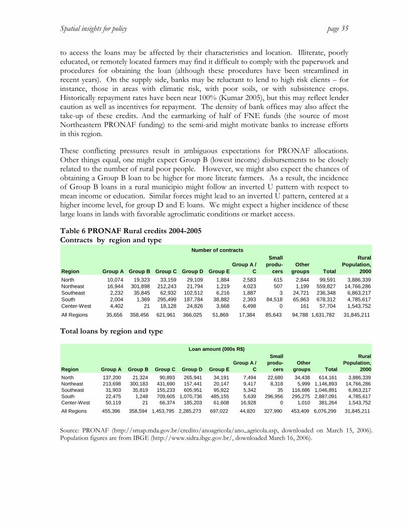
Spatial insights for policy page 35
to access the loans may be affected by their characteristics and location. Illiterate, poorly educated, or remotely located farmers may find it difficult to comply with the paperwork and procedures for obtaining the loan (although these procedures have been streamlined in recent years). On the supply side, banks may be reluctant to lend to high risk clients – for instance, those in areas with climatic risk, with poor soils, or with subsistence crops. Historically repayment rates have been near 100% (Kumar 2005), but this may reflect lender caution as well as incentives for repayment. The density of bank offices may also affect the take-up of these credits. And the earmarking of half of FNE funds (the source of most Northeastern PRONAF funding) to the semi-arid might motivate banks to increase efforts in this region.
These conflicting pressures result in ambiguous expectations for PRONAF allocations. Other things equal, one might expect Group B (lowest income) disbursements to be closely related to the number of rural poor people. However, we might also expect the chances of obtaining a Group B loan to be higher for more literate farmers. As a result, the incidence of Group B loans in a rural municipio might follow an inverted U pattern with respect to mean income or education. Similar forces might lead to an inverted U pattern, centered at a higher income level, for group D and E loans. We might expect a higher incidence of these large loans in lands with favorable agroclimatic conditions or market access.
Table 6 PRONAF Rural credits 2004-2005 Contracts by region and type
Region Group A Group B Group C Group D Group EGroup A /
C
Small produ-
cersOther
groups Total
Rural Population,
2000
North 10,074 19,323 33,159 29,109 1,884 2,583 615 2,844 99,591 3,886,339Northeast 16,944 301,898 212,243 21,794 1,219 4,023 507 1,199 559,827 14,766,286Southeast 2,232 35,845 62,932 102,512 6,216 1,887 3 24,721 236,348 6,863,217South 2,004 1,369 295,499 187,784 38,882 2,393 84,518 65,863 678,312 4,785,617Center-West 4,402 21 18,128 24,826 3,668 6,498 0 161 57,704 1,543,752
All Regions 35,656 358,456 621,961 366,025 51,869 17,384 85,643 94,788 1,631,782 31,845,211
Number of contracts
Total loans by region and type
Region Group A Group B Group C Group D Group EGroup A /
C
Small produ-
cersOther
groups Total
Rural Population,
2000
North 137,200 21,324 90,893 265,941 34,191 7,494 22,680 34,438 614,161 3,886,339Northeast 213,698 300,183 431,690 157,441 20,147 9,417 8,318 5,999 1,146,893 14,766,286Southeast 31,903 35,819 155,233 605,951 95,922 5,342 35 116,686 1,046,891 6,863,217South 22,475 1,248 709,605 1,070,736 485,155 5,639 296,956 295,275 2,887,091 4,785,617Center-West 50,119 21 66,374 185,203 61,608 16,928 0 1,010 381,264 1,543,752
All Regions 455,396 358,594 1,453,795 2,285,273 697,022 44,820 327,990 453,409 6,076,299 31,845,211
Loan amount (000s R$)
Source: PRONAF (http://smap.mda.gov.br/credito/anoagricola/ano_agricola.asp, downloaded on March 15, 2006). Population figures are from IBGE (http://www.sidra.ibge.gov.br/, downloaded March 16, 2006).

Spatial insights for policy page 36
We look first, and briefly, at national allocations of PRONAF credits for 2005 (See Table 6). There is a distinct pattern. The nation’s wealthiest region, the South, receives 42% of the total contracts and 48% of the total funds, but has only 18% of rural workers10. It has about half the Group C contracts and credits, but only 19% of rural workers earning between 0.5 and 5 minimum salaries. This pattern likely reflects a combination of higher landownership rates and less unequal landholdings, more educated farmers, more productive and credit-worthy farms embedded in more effective marketing networks, and more active outreach by extension and bank agents. A further decomposition of these contributing factors might provide insight into ways of increasing credit take-up in the Northeast.
Figure 17 Incidence of PRONAF credits (group B and C) in the Northeast
Note: Contracts for 2004-05 divided by rural population in 2000. Source: PRONAF (http://smap.mda.gov.br/credito/anoagricola/ano_agricola.asp, downloaded March 8,2006)
10 Based on PNAD, 2004, table 1867

Spatial insights for policy page 37
Next we look at PRONAF allocation within the Northeast, focusing on loans taken by low-income Groups B and C. Figure 17 shows the ratio of contracts to rural population for 2004-05. There is considerable spatial variation in the incidence of contracts, but no obvious pattern, aside from high incidence in western Rio Grande do Norte. Table 7 reports a regression of contract incidence by municipio on poverty rates, illiteracy rates, urbanization rates, location in the semi-arid, and presence of major irrigation works. The regression equation has very little explanatory power. However, it shows that, other things equal, location in the less-difficult semi-arid boosts contract incidence by 7.6 per hundred rural people compared to the non-semi-arid – an amount higher than the mean incidence. Presence in the more-difficult semi-arid has a smaller incremental effect, about 5 per hundred compared to the non-semi-arid. There is a slight inverse U relationship between incidence and illiteracy. Incidence is U shaped with respect to urban proportion11.
Table 7 Determinants of PRONAF credit allocation in the Northeast
Variable Coef. t-stat
Chg in dep var
for 2 std dev chg
in this var
F-test prob for
joint signif Mean
Std. Dev. Min Max
Type B or C contracts in 2005 per rural person 0.0619 0.3919 0 16.0588
Private irrigation proportion 0.0064 0.04 0.0007 0.9989 0.0179 0.0557 0 0.5598Public irrigation proportion -0.0366 -0.13 -0.0024 0.0042 0.0331 0 0.6964Proposed irrigation proportion -0.0245 -0.08 -0.0015 0.0030 0.0306 0 0.6996More difficult agroclimate 0.0492 2.09 0.0416 0.0065 0.3221 0.4224 0 1Less difficult agroclimate 0.0760 3.00 0.0606 0.2774 0.3988 0 1Illiteracy rate, 2000 2.48E-02 3.33 0.0262 0.0029 43.40 9.18 7.28 70.13 - squared -2.70E-04 -3.14Indigency rate, 2000 5.61E-03 0.94 0.0259 0.5077 43.77 11.04 5.82 81.65 - squared -5.07E-05 -0.78Proportion urban, 2000 -1.1878 -5.21 0.1066 0.0000 0.4963 0.2019 0.0156 0.99959 - squared 1.4624 6.59Constant -0.4948 -3.25
R-squared 0.0406
Source: PRONAF (http://smap.mda.gov.br/credito/anoagricola/ano_agricola.asp, downloaded on March 8, 2006)
Given the very large amount of resources devoted to PRONAF, it would be useful to better understand the factors that shape the spatial allocation of these resources and in particular the lack of a clear relationship to the poverty rate. Differentials in access to land may be an important factor; supply-side activities might also be important.
11 Some urban dwellers in small towns may qualify for PRONAF credits based on nearby farms. In municipios with high urban proportions, the number of rural dwellers may be a poor proxy for the number of people engaged in farming.

Spatial insights for policy page 38
3. UNDERSTANDING SPATIAL DIFFERENCES IN ECONOMIC PERFORMANCE
Why do lagging regions lag? Lagging regions such as Brazil’s are often characterized by a syndrome of overlapping constraints: poor agroclimatic conditions, remoteness from markets, lack of education, lack of infrastructure and other physical capital, poor governance. These constraints can be mutually reinforcing, for reasons explained in the previous section. This makes it difficult to understand how to intervene.
This section tries to disentangle the effects of these overlapping constraints, emphasizing their effect on Northeast Brazil. To set the stage, it first looks nationwide at spatial changes in labor markets over the period 1991-2000. The goal is to elucidate the processes which generated the heterogeneous patterns shown in Figure 18: substantial spatial variation in outcomes, but generally poor performance in the Northeast. Then it focuses specifically on the Northeast compared to other regions. It provides a geographically detailed accounting of people subject to different degrees of agroclimatic constraints in the Northeast. It then assesses the relationship between these agroclimatic conditions and various measures of poverty. It then examines the determinants of labor market outcomes within the Northeast, in order to distinguish the relative effect of policies and geographical conditions. Finally, it looks in particular at the implications of variability in rainfall for economic conditions.
WHAT ACCOUNTS FOR DIFFERENTIAL LABOR MARKET PERFORMANCE BETWEEN
MUNICIPIOS?12
This section examines in more detail the causes, correlates and implications of the heterogeneous labor market patterns shown in Figure 18. What drives the observed patterns, especially the contrast between stagnant markets in the North and Northeast, and more vibrant ones in the South? What kinds of policies might be associated with growth in labor demand? What are the implications for high poverty density vs. high poverty rate areas? The results presented here come out of joint work undertaken with IPEA, presented in Chomitz, da Mata, Carvalho, and Magalhaes .(2005a) (CMCM). There is a substantial and growing literature which applies traditional Barro-type growth models (Barro 1991) to state level data for Brazil, with the goal of understanding whether or not Northeastern incomes are converging towards national level. There is some evidence of convergence in incomes between states over the periods 1939-1985 (Azzoni 2001) (and 1970-1985 (Ferreira and Diniz 1995). However, several papers find evidence that this convergence process stalled after 1985, with one or two groups of poor states tending towards a lower-income equilibrium than the richer part of Brazil. ((Azzoni 2001); Ferreira 1998; Pontual e Porto Júnior 2000;(AZZONI et al. 2000)
12 The section is largely based on Chomitz, da Mata, Carvalho, and Magalhaes (2005) (CMCM), quoting, in some cases verbatim, tables, maps, and results.

Spatial insights for policy page 39
A highly disaggregate spatial labor market approach can help to elucidate the reasons for divergence. The labor market approach has several advantages over Barro-type growth models. First, it offers potentially better insight into poverty alleviation strategies because it looks at wages rather than GDP/capita – an important consideration when wealth is unequally distributed, or when value-added accrues to absentee landlords13. Second, the growth models tend to look only at mean income or output of regions, implicitly endorsing an emphasis on comparison between units rather than individuals. It is entirely possible for regional mean incomes to diverge even while incomes of individuals increase, if employment expands faster in higher-wage markets. Models focused only on mean income may entirely overlook such an outcome. Third, growth models typically employ a sparse set of policy-relevant variables. The analysis considers the impact of a range of policy levers, including education, infrastructure, and transfers, while allowing for differential effects in regions with different agroclimatic conditions. Finally, a fine-scaled geographic approach facilitates an examination of local growth spillovers, allowing examination of the premises of territorial development policies.
Figure 18 and Table 8 segment the landscape14 into four types of areas:
Booming employment, declining wages (E+W-). These areas, in which employment grew more rapidly than population, but real wages declined, may include areas of economic stagnation. Here, labor demand failed to keep up with the growth of supply. This reflects, in part, natural increase; the mean total fertility rate for the E+W- areas was 3.78 in 1991, far above the other three categories. However, some of these areas are also apparently attracting in-migrants more rapidly than they can provide jobs, with about one-fifth of the population arriving in the previous decade. By 2000, about 22% of employed workers lived in the E+W- areas. They account for a particularly large share of population (though a small absolute number) in the North. It is possible that E+W- areas in frontier regions of the North are not in fact stagnant, but are witnessing rapid growth from a small base, and a wage decline from anomalous, disequilibrium levels.
Dynamic areas with both increasing wage growth and rapidly increasing employment (W+E+). These areas had 32% of Brazilian employment in 1991, but absorbed 53% of the country’s net increase in employment, while registering an increase in average real earnings. Such an outcome may reflect a relative shift outward in the labor demand curve. Although the 1991 total fertility rate for these MCAs was a full point lower than that of the E+W- areas, the dynamic areas had a substantial higher proportion of recent immigrants in 2000; this suggests that these regions are growing via immigration, presumably drawn by economic opportunity.
13 Nonetheless, labor market analysis results can be compared with those of growth regressions by taking wage growth as a proxy for productivity growth and employment as a proxy for município size.
14 The unit of analysis is the MCA, Minimum Comparable Area. If a municipios is unchanged between 1991 and 2000, it constitutes an MCA. When municipios split and/or recombine, they are aggregated into the smallest constant unit.

Spatial insights for policy page 40
Declining areas (E-W-) with falling real wages and slower than average employment growth. These may be areas where labor demand has dropped substantially.
(i) Booming wage, declining employment areas (E-W+) appear to have sluggish or declining labor supply. These largely metropolitan areas are characterized by both low fertility rates and low in-migration rates.
Figure 18 Labor dynamics 1991-2000
Source: Chomitz, da Mata, Carvalho, Magalhaes 2005
Table 8 Employment trends by labor market outcome
Employment growth
Population Growth Frequency
Quadrant 1991 2000 1991 2000 1991 2000E+, W+ 14707336 19090991 4383655 40% 43% 37785537 47940239 10154702 332E-, W+ 10144794 10924107 779313 27% 25% 25298240 27583837 2285597 154E-, W- 6188863 6547091 358228 17% 15% 15430178 16591747 1161569 73E-, W- 5978230 7957879 1979649 16% 18% 16504563 21302846 4798283 176Total 37021214 44522068 7500854 100% 100% 95018518 113420669 18402151 735
Metropolitan Areas
Employment PopulationEmployment Share

Spatial insights for policy page 41
Employment growth
Population Growth Frequency
Quadrant 1991 2000 1991 2000 1991 2000E+, W+ 3481048 4551220 1070172 19% 22% 9300552 10991493 1690941 701E-, W+ 5949685 5950681 996 33% 28% 15123906 15312581 188675 1172E-, W- 4005760 4008645 2885 22% 19% 11833148 11888764 55616 743E-, W- 4837597 6599279 1761682 26% 31% 15549351 18187663 2638312 916Total 18276081 21111825 2835744 100% 100% 51806957 56382501 4575544 3532
Population
Nonmetropolitan Areas
Employment Employment Share
Employment growth
Population Growth Frequency
Quadrant 1991 2000 1991 2000 1991 2000���◊ W+ 18188385 23642211 5453826 32% 35% 47086089 58931732 11845643 1033���◊ W+ 16094479 16874788 780309 28% 25% 40422146 42896418 2474272 1326���◊ W- 10194623 10555736 361113 19% 17% 27263326 28480511 1217185 816���◊ W- 10815827 14557158 3741331 22% 23% 32053914 39490509 7436595 1092Total 55295305 65631893 10336588 100% 100% 146825475 169801170 22975695 4267
Employment PopulationShare of employment
All Areas
Source: Chomitz, da Mata, Carvalho, Magalhaes 2005
Table 8 shows that metropolitan areas account for about two thirds of employment. Dynamic (W+E+) metropolitan areas absorbed 43% of the nation’s net growth in employment; about 43% of the metropolitan labor force was in a dynamic area. In contrast, stagnant (W-E+) areas are much more prevalent in the nonmetropolitan areas, comprising 31% of the nonmetropolitan workforce. Among the regions, the Center West is the most dynamic, with nearly 70% of its population living in E+W+ MCAs. Employment in these Center West areas appears to be growing in large part due to in-migration. The proportion of in-migrants (at the municipio level) was about 30%, the highest of the five regions. In comparison, the Northeast’s proportion was 16%, the lowest.
Explaining the patterns
CMCM estimated spatial labor supply and demand equations to analyze the employment and wage outcomes shown in Figure 18. The labor demand equation relates change in average wages, by MCA, to:
• Changes in employment • initial levels of human, social and geographic capital (education, teacher
qualification, rainfall, transport costs to São Paulo and to the nearest state capital, use of computers for keeping municipal financial accounts as a proxy for government quality and accountability)
• changes in the income of neighboring municipios – a proxy for demand spillovers

Spatial insights for policy page 42
• changes in the amount of government transfers to individuals in the municipio
The labor supply equation expressed change in employment as a function of:
• initial wage rates • initial demographic conditions (including the relative size of the cohort
entering the labor market) • initial proportion in farming • local amenities (teacher qualifications, homicide rates, presence of a bank) • changes in the income of neighboring municipios (here a proxy affecting
relative wages) The estimation procedure allowed for the endogeneity of explanatory variables. Importantly, the procedure allowed for spatial autocorrelation of errors, recognizing that outcomes in small, adjacent municipios could reflect the presence of some unobserved factor common to both15. Estimates were made for all of Brazil, for nonmetropolitan Brazil (i.e. excluding the largest urban areas), and for nonmetropolitan Brazil excluding the North region. Results were found to be robust to the choice of sample and to differing adjustments for spatial autocorrelation. For methodological details, see CMCM.
The results are reproduced in Appendix Table 5. The chief findings were as follows.
Initial levels of workforce education are highly correlated with subsequent wage growth. Figure 19 shows a remarkable bivariate correlation between worker education in 1991 and wage growth over the period 1991-2000. CMCM show that the correlation persists even after controlling for climate, remoteness, and a crude proxy for local governmental capability. Each additional year of mean worker education is associated with an increment of 6% to 7% in the nine-year growth rate of wages. The result is highly statistically significant. Taken at face value, it implies that the mean educational level of a community workforce accelerates subsequent productivity growth in that community. The red points represent AMCs of the North and Northeast, while the blue ones are from the rest of the country. There is a remarkable disjunction in educational levels between the two parts of the country, and this disjunction is highly correlated with the differentials in wage growth shown in Figure 18.
15 See Carvalho, da Mata, Chomitz (2005) for a description and assessment of this technique, due to Conley (1999)

Spatial insights for policy page 43
Figure 19 Education and earnings growth, Brazil
Source: CMCM Blue – Southeast, South and Center-West Regions Red – North and Northeast Regions. This dynamic relationship between education levels and subsequent wage growth is different from the standard human capital relationship between education level and wage level. The North and Northeast of the country lag far behind other regions in quantity and quality of education, and these differentials are strongly correlated with differences in labor income, as human capital theory would suggest (Fiess and Werner 2004). Montalverne Ferreira and Salvato (2004) find that education alone accounts for 55% of the earnings differential between the Northeast and Southeast. However, education and other observable individual characteristics do not fully explain cross-sectional wage and income differentials. Fiess and Werner, for instance, estimated that low-education Northeasterners could boost their wages by 80% through migration. Azzoni and Santos (2002) compared the differences in salary in the 10 largest Brazilian metropolitan areas in 1992, 1995 and 1997. Those salary differences remained significant even after controlling for cost of living measures, the traits of the workers (education, age, sex, race and family position) and the traits of their jobs (occupational position, sector and experience).
The dynamic relationship found here does not necessarily imply a causal link from education to subsequent wage growth. It is possible, for instance, that some common third factor affects both educational level and wage growth. For instance, some places may have a local tradition of social or cultural capital that encourages both educational investment and entrepreneurship. Because social and cultural capital are difficult to measure, this explanation is difficult to refute. Nevertheless, it is plausible that the mean educational level

Spatial insights for policy page 44
of a community does influence subsequent wage growth. One would expect more-educated communities to be more adaptable to changes in economic conditions, more likely to invest in formal education and training (at the household and community level), and better able to monitor the performance of local officials. Higher community levels of education may in fact catalyze the formation of social capital.
Farming regions are losing employment, or growing more slowly than other regions. This result is in addition to migration associated with wage differentials. In the nationwide sample, each 10 percentage point increase in the initial proportion of farmers among workers was associated with a 10 to 12 percent decrease in the nine-year rate of employment growth. Even when the sample is restricted to nonmetropolitan areas, this relationship holds, though it is less steep. Further investigation is needed to understand the degree to which this represents ‘pull’ factors – attraction to growing areas, vs. ‘push’ factors – e.g. displacement of smallholders by large farming enterprises.
Low rainfall areas lagged other areas in wage and employment growth. These patterns were evident even controlling for remoteness and education, which might be correlated with rainfall. A 1000 mm increase in rainfall was associated with approximately 10% higher wage growth over the nine year period.
Wages respond relatively elastically to changes in labor supply. A 10% increase in labor supply will reduce wages, other things equal, by 7% to 8%. This helps to explain wage stagnation in areas with high rates of natural increase. It also underlines the remarkable achievement of the dynamic areas (W+E+) in maintaining or improving real wages in the face of substantial employment increases. And it emphasizes that the economic performance of localities or regions should not be judged solely on wage growth, since employment absorption will tend to depress wages.
There appear to be positive spillover effects on wages and employment from income growth in nearby areas. CMCM’s estimates suggest that for nonmetropolitan areas a 10% increase in close neighboring regions’ income is associated with a 7% increase in own wages and a 2% increase in employment. The estimate took pains to reduce the possibility that this effect was duet to a correlation with unobserved favorable factors common to the município and its environs, though these controls may not have been fully adequate. The finding supports a territorial development approach which advocates stimulating the growth of small cities in order to benefit nearby neighbors. Whether or not it is possible, in fact, to spur the growth of such cities is a different question.
Government transfers – such as pensions—are associated with more rapid local wage growth. More rapid growth in receipt of transfers is associated with more rapid wage growth. Much of the growth in transfers over the 1990’s is associated with a expansion of rural pension coverage, including expansion of coverage to women and a reduction in the eligibility age. There are two possible ways this expansion might boost wages. First, it might be a

Spatial insights for policy page 45
compositional effect. The expansion of pensions encouraged older workers to withdraw from the labor force. If their earnings were lower than average, this would boost the measured mean wage. Second, it is possible that such transfers result in favorable local multiplier effects, as the pensioners increase their demand for local goods such as services and some foodstuffs.
TO WHAT EXTENT DO POOR AGROCLIMATIC CONDITIONS CONSTRAIN NORTHEASTERN
GROWTH?
Much of the area of semi-arid Northeastern Brazil falls into the high poverty rate, low poverty density category. Clearly, places in the semi-arid region face a variety of special constraints and challenges. Low population density is already a challenge, but the low population density reflects a low carrying capacity of the land and high vulnerability to climate shocks, including droughts and floods. This suggests that it would be useful to target specifically-designed interventions to the most constrained people and places.
Agroclimate and investments
To establish context, we draw on the literature review by Kelley and Byerlee (2003) of agricultural prospects and challenges in less favored regions. The literature is relatively thin and lacking in hard numbers.
A few general principles appear to be clear. First, providing agriculture extension services for remote rural communities is difficult, very costly, and the returns to investment are affected by geographical patterns. According to Anderson and Feder (2003), “the clients of extension services live in geographically dispersed communities, where the transport links are often of low quality, adding to the cost of reaching them. The incidence of illiteracy and the limited connections to electronic mass media can further limit the ability to reach clients via means that do not require face-to-face interaction (e.g., written materials, radio, television, internet).” Mitch (2000) suggests that the economic return to extension services should,“[al]most by definition”, find that the impact of these services is higher in favored areas vis-à-vis to marginal areas (remote, endowed with inferior infrastructure or institutional inadequacies, and poorer availability and higher cost of complementary inputs). (See also ARD, 2004; Evenson, 1997).
Second, agricultural research and development directed towards the agroclimatic situation of less-favored zones can have profound impacts and offer potentially very high rates of return. For instance, Kelley and Byerlee report that improved cassava varieties boosted Nigerian per capita income by 10%, and biocontrol of cassava mealy-bug has benefited farmers and consumers throughout subSaharan Africa.
Third, irrigation provides variable benefits, depending both on the institutional and environmental context. Small-scale irrigation in Nigeria has shifted farmers from subsistence grains to vegetables (Kelley and Byerlee 2003). In Northeast Brazil, a recent study of 11 irrigation districts found rates of return to investment of 8.9% to 25.4% (compared to social discount rates of 16.8% to 19.1%) (World Bank 2004) Varying results were ascribed largely to management or institutional factors. The study also compared municipalities with irrigation projects to matched municipalities without. The irrigated municipalities

Spatial insights for policy page 46
experienced much greater growth in population; they maintained (but did not widen) an advantage in income per capita. This suggests substantial poverty reduction impacts, realized through in-migration.
Interesting evidence on returns to investment in different agroclimatic zones is provided by an analysis of the Cedula da Terra project in Northeast Brazil. This project financed Land Purchase for 15,000 poor farm families organized into community associations; Community subprojects for those same beneficiary groups, through small matching grants for investments, technical assistance and start-up; and Community Development Support, Technical Assistance and Training (institution building) through consulting services and training, and public dissemination of information about the project. Estimated total project cost was US$150.0 million (World Bank 2003)
The analysis of the Cedula da Terra impact found that the economic and financial rates of return are much lower in geographically disadvantaged areas. The study found a 21% rate of economic return to investment for the Semi-arid, which is characterized by insufficient rainfall and subsistence agriculture (including livestock) activities, compared to 27% in the Meio-Norte, which is characterized by increased rainfall and minimal irrigation systems, and to 55% in the Zona da Mata, which is characterized by sufficient rainfall and overall favorable climatic conditions (World Bank 2003).
Fan et al. (2000) looked at the impact of canal irrigation, education, high-yielding varieties and electricity across 14 agroclimatic zones of India. They found the highest returns to education in the least-favored rainfed zones – perhaps because of a low base. However, they found an inverse-U relationship between agroclimatic conditions and the effect of road investments on poverty alleviation. They found that a million rupee investment in roads reduces poverty by 8 individuals in irrigated areas, by 25 to 55 in the five most favorable rainfed zones, by (a possibly anomalous) 165 in the sixth zone, and by 0 to 25 in the seven least favorable zones. The irrigated areas may have already been well provided with roads, so this suggests that road investments have a higher impact in more favorable rainfed areas than in the least favorable ones.
How many people live in agro-climatically constrained areas in the Northeast?
For policy purposes it is important to know how many people are subject to agro-climatic constraints, and the relative importance of agro-climatic versus other kinds of constraints. If agro-climatic constraints are both important and geographically localized, this might support tightly targeted spatial interventions.
To quantify the affected population, we combined census-tract level data from the 1991 and 2000 Demographic Censuses with detailed agroclimatic data. For each year, census tract boundaries were overlaid on other maps, allowing population to be cross-classified according to the following criteria (shown in Figure 20)
• Geophysical definition of the semi-arid, distinguishing the “more difficult areas” (the Depressão Sertaneja – or sertões – and the maciços serranos residuais) from “less difficult areas”, following a classification by FUNCEME (FUNCEME/ETENE 2004). The former areas are roughly equivalent to the

Spatial insights for policy page 47
caatinga. The semi-arid areas defined here have a high degree of overlap with low rainfall areas.
• Soil type --a simple binary classification by FUNCEME, based on fertility and water holding capacity
Figure 20 Northeast: Semi-arid areas, soils, rivers and urban settlements
Source: authors’ mapping of data assembled by FUNCEME (panels 1-3) and IBGE (panel 4)

Spatial insights for policy page 48
• Proximity (within 2 km) to a permanent river or major reservoir. Note that many irrigation works fall outside of this geographical criterion.
• Urban-rural location, using the Census categories to distinguish between dispersed rural populations, rural ‘agglomerations’ (very small settlements), and ‘urban’ areas, keeping in mind that the Census includes as ‘urban’ relatively small towns (perhaps with populations of 1000 or less) located in a rural landscape.
Table 9 and Figure 21 show the number of Northeastern residents falling into different combinations of these constraints, for 1991 and for 2000. (The tabulation is restricted to the Census definition of the Northeast Region and excludes the semi-arid portions of Minas Gerais.) The most striking finding is the decline in the number and proportion of dispersed rural dwellers in the semi-arid regions – the group presumed to be poorest and most vulnerable. In 1991, the semiarid population constituted about 45% of the Northeast’s population, a proportion which stayed approximately constant over the next decade. In constrast, the proportion of the semi-arid population which lives in dispersed rural conditions and more than 2 km from rivers or reservoirs declined from 43% to 36%. In absolute terms, this population declined 10%, from 8.3 million to 7.5 million. The number of people living in the most difficult conditions – on poor soils in the sertões, and not adjacent to rivers or reservoirs – declined 12%, from 2.2 to 2.0 million. Conversely, the
Figure 21 Rural population declined in the semi-arid between 1991 and 2000
0 1,000,000 2,000,000 3,000,000 4,000,000 5,000,000 6,000,000 7,000,000
LD rural bad soil
LD rural good soil
LD village
LD urban
MD rural bad soil
MD rural good soil
MD village
MD urban
near reservoir/river
Population
2000
1991
Key: LD – ‘less difficult’ semi-arid; MD – ‘more difficult’ semi-arid Source: authors’ calculations

Spatial insights for policy page 49
Table 9 Northeastern population by agroclimatic constraints, 1991 and 2000 Location type of settlement 1991 2000 Change NONSEMIARID 23,409,308 26,967,633 15.2% SEMIARID (except within 2 km of reservoir or major river) Less Difficult dispersed rural LD rural bad soil 1,097,485 954,732 -13.0%
LD rural good soil 2,831,034 2,524,628 -10.8% rural agglomerations LD village 466,550 543,427 16.5% urban LD urban 5,031,218 6,242,963 24.1%
More difficult dispersed rural MD rural bad soil 2,262,527 1,989,571 -12.1% MD rural good soil 2,099,185 1,987,182 -5.3% rural agglomerations MD village 400,215 479,643 19.8% urban MD urban 3,934,732 4,842,481 23.1%
SEMIARID (within 2 km of reservoir or major river)
near reservoir/river 959,170 1,084,471 13.1%
TOTALSEMIARID 19,082,116 20,649,097 TOTAL MAPPED POPULATION 42,491,424 47,616,730
Note: some populations could not be mapped to census tracts. 1991 unmapped population: 11938, all outside the semiarid.; 2000 unmapped population: 139074, of whom 26486 are outside the semiarid and 84163 are in more difficult,bad soil, far from reservoir areas. Source: authors’ calculations based on Censo Demographico. number of semi-arid urban dwellers increased by about 25%, reaching over 11 million in 2000 – again excluding areas adjacent to major rivers.
Figure 22 Population in "Extremely High Priority" areas for Caatinga biodiversity
Source: own calculations based on IBGE and biodiversity focus groups

Spatial insights for policy page 50
Another aspect of constraints has to do with the presence of threatened biodiversity. The caatinga, which corresponds roughly with the ‘more difficult’ areas of the semi-arid, is considered of global importance for its unique and threatened biodiversity. Using census tract level data we calculate that there are about 1.3 million dispersed rural dwellers living in “Extremely High Priority” biodiversity areas, as classified by an expert workshop(Universidade Federal de Pernambuco 2002). (See Figure 22).
What is the relation between agro-climatic constraints and poverty?
Analysis of municipio-level Census data suggests that education and urban residence are much more important correlates of cash income than location in the sertão or other semi-arid. Figure 23 relates the indigency rate (proportion of people living at less than quarter minimum wage, based on cash income) to the mean education of workers, for municipios outside of metropolitan areas. (The left hand graph is a smoothed running average of the scatters shown on the right.) On average, increases in education are associated with steep declines in the proportion indigent. But controlling for education, there is little difference in the indigency rates between the more difficult semi-arid, the less difficult semi-arid, and areas outside the semi-arid. Figure 24 shows a similar graph for urban proportion. The graph excludes metropolitan areas, so that ‘urban’ refers to small towns. Even at this scale there is a very strong association between urban proportion and indigency rate, with relatively minor differentials between agroclimatic zones. Figure 25 shows the relationship between mean worker education and mean ln wage. As we would expect, wages are strongly associated with education. But holding education constant, workers earn significantly less in semi-arid areas. Note that in all these cases, a full income accounting, allowing for the value of self-produced food and goods, would tend to reduce the differentials between rural and urban, or low vs. high education.
Figure 23 Poverty is strongly inversely related to education
Source: own calculations
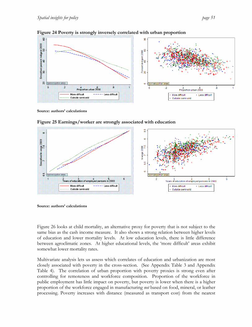
Spatial insights for policy page 51
Figure 24 Poverty is strongly inversely correlated with urban proportion
Source: authors’ calculations
Figure 25 Earnings/worker are strongly associated with education
Source: authors’ calculations
Figure 26 looks at child mortality, an alternative proxy for poverty that is not subject to the same bias as the cash income measure. It also shows a strong relation between higher levels of education and lower mortality levels. At low education levels, there is little difference between agroclimatic zones. At higher educational levels, the ‘more difficult’ areas exhibit somewhat lower mortality rates.
Multivariate analysis lets us assess which correlates of education and urbanization are most closely associated with poverty in the cross-section. (See Appendix Table 3 and Appendix Table 4). The correlation of urban proportion with poverty proxies is strong even after controlling for remoteness and workforce composition. Proportion of the workforce in public employment has little impact on poverty, but poverty is lower when there is a higher proportion of the workforce engaged in manufacturing not based on food, mineral, or leather processing. Poverty increases with distance (measured as transport cost) from the nearest

Spatial insights for policy page 52
state capital and from Sao Paulo. The correlation of education with poverty is vitiated when the proportion of children in the population is included. (This is itself highly correlated with lower educational levels.) Controlling for these and other factors, the indigency rate in the ‘more difficult’ semi-arid is about 3.5 percentage points higher – about one third of a standard deviation.
Reductions in the indigency rate between 1991 and 2000 are strongly related to increases in transfers per capita (see Figure 27). For most of the range of the change in transfers, there is little difference between agroclimatic regions in this relationship. (There are few AMCs outside the semi-arid with increases over R$15, so the apparent divergence at high transfers is misleading.) Increases in measured education per worker are not much associated with reductions in indigency rates, but the educational changes, as the difference between two imperfectly measured values, are subject to large measurement error.
Figure 26 Child mortality declines with education
Source: own calculations

Spatial insights for policy page 53
Figure 27 Increased transfers are associated with decreased indigency
Source: own calculations
Geographic and policy determinants of labor market changes in the Northeast
These descriptive correlations motivate a labor market analysis similar to the national one discussed earlier. In a companion piece to CMCM, Carvalho, Chomitz and da Mata (CCM) modeled labor market outcomes in the Northeast. In contrast to CMCM, CCM estimate a reduced-form model of wage and employment growth in the Northeast. The Northeast analysis accounts for the effect of agroclimatic location indicators, rainfall, and the area of public or private irrigation in 1989. The analyses yield similar results regardless of whether the metropolitan areas are included. Here, results excluding the metropolitan areas are reported.
Wage (earnings/worker) growth and employment growth were modeled as a function of variables affecting changes in supply and demand, with controls for spatial autocorrelation and instruments for endogenous variables. (See regression results in Appendix Table 6). Results broadly paralleled those for the national study:
o Again initial levels of worker education were important in determining subsequent wage growth: each year of additional education was associated with approximately 8% wage growth over the subsequent nine years.
o Increases in transfers per worker strongly increased mean wages (elasticity of .94) but strongly reduced employment growth (elasticity of -.57). This is consistent with a reduction in labor force supply by old-age rural pensioners. The increase in average

Spatial insights for policy page 54
earnings may simply reflect the withdrawal of this low-earning group, but it may to some extent reflect increased local earnings of others due to a local multiplier effect of spending by pensioners.
o Growth in income of neighboring areas strongly increased the growth of wages and had a similarly large, but not quite statistically significant on local employment growth. This provides some evidence for spillover effects of regional development.
o High initial proportion of workforce in farming strongly depressed wage growth, but in contrast to the national results had little effect on employment growth. However, high income inequality was strongly related to low or negative change in employment.
o Interestingly, the change in local public employment had no effect on earnings or employment growth.
o Remoteness from the nearest state capital was strongly associated with lower wage growth
o Proportion of area under private irrigation in 1989 boosted wage growth but not employment growth. The effect on wages may reflect the endogeneity of wage growth. Proportion of area under public irrigation in 1989 affected neither. At first glance this appears to contradict (World Bank 2004), which found rapid relative employment growth in municipios with irrigation, compared to similar municipios without. However, the regression analysis treats each AMC as a separate experiment. Most of the employment growth associated with irrigation was apparently recorded in a relatively few places. This underlines the World Bank study’s finding of great variability between locations in the success and rapidity of irrigation-led development.
o Controlling for these effects, location in the semi-arid depressed nine-year wage growth by about 20% - a substantial amount. The effects were about the same in the more and less difficult areas. Controlling for these locations, rainfall and soil had no significant effect.
Economic vulnerability to weather shocks16
The most problematic feature of the semi-arid for poverty and development is not the low mean level of rainfall, but the extreme variability of rainfall. The region is subject to both droughts and floods, and either extreme can lead to crop failures and other hardships. These weather shocks cause direct economic losses. Adaptation to climate volatility might either exacerbate or dampen the sensitivity of the economy to the weather shocks. Theoretically, one would expect risk-averse farmers to adapt to volatility by choosing low-yielding but less weather-sensitive livelihood strategies – deepening their poverty but insulating them somewhat from year-to-year shocks. On the other hand, reliance on drought relief may encourage use of more weather-sensitive
16 This represents initial results from work in progress with IPECE.

Spatial insights for policy page 55
strategies. And the growing use of ultra-small reservoirs may encourage overexpansion of agriculture in more favorable years, leading to crashes in drought years.
To assess the sensitivity of local economies to weather shocks, we took advantage of data from FUNCEME’s dense network of weather stations in Ceará, with a station in nearly every municipio. We merged annual rainfall data by municipio for 1997-2004 with agricultural GDP data furnished by IPECE and with geophysical, biophysical, and infrastructure data assembled by FUNCEME. We estimated the following equation describing the agricultural GDP of municipio i at time t:
ln AgGDPit = µi +ηt +β1rit+β2rit2+β3rit
3+ uit
where rit = is the deviation of the ln rainfall in municipio i, year t from the ln mean for the municipio over the eight year observation period. The first two terms allow for systematic differences between municipios and for year-to-year macroeconomic shocks. The three terms in r allow for a wide range of responses to weather shocks. We hypothesized, however, that agricultural output would decline with either positive or negative shocks. To test whether there were significant differences in climate sensitivity between more and less arid regions, we estimated this equation for two separate sets of municipios: those with more than 50% of their territory in the caatinga biome, and those with less than 10% of their territory in the caatinga. (The caatinga biome definition – see Figure 28 -- is based on potential vegetation, not current land cover.) The caatinga biome is a good proxy for low and variable rainfall conditions. In both cases we excluded municipios with large irrigation works, or with urban areas of greater than 20000 people in 2000.
Preliminary results of estimation are shown in Table 10. There are substantial annual effects independent of weather; 2001 was a very poor year in both subregions, while 2003 was a favorable year for the caatinga, holding weather constant. Rainfall deviations, surprisingly, have no statistically significant effect on agricultural GDP in the non-caatinga municipios.
However, the caatinga municipios exhibited strong, statistically significant sensitivity to weather shocks. The predicted effect of rainfall deviations in the caatinga is shown in Figure 29. Each curve represents the predicted effect of rainfall deviations for a particular year, and each point represents an actual observation of a rainfall deviation for that year. The graph shows that, controlling for macroeconomic conditions, maximum agricultural GDP is associated with near-mean rainfall. Higher or lower levels of rainfall substantially depress GDP. Rainfall 20% below average (which is not uncommon) is associated with a 5% reduction in agricultural GDP. Note that these impacts, while substantial, are smaller than the year to year variation due to macroeconomic effects. But those ‘macro’ may themselves reflect the repercussions of state-wide or region-wide weather. Note that the year with poorest performance has a lopsided distribution of weather shocks: almost all are negative.

Spatial insights for policy page 56
Figure 28 Ceará: caatinga and population density
Source: mapped by authors using data compiled by FUNCEME; population data from HDI
Figure 29 Impact of weather shocks on agriculture in the Ceará caatinga
Note: curves correspond to different years; Source: authors’ estimates

Spatial insights for policy page 57
Table 10 Sensitivity of local agricultural GDP to weather: regression estimates
Caatinga nonCaatinga observations 320 360 municipios 40 45 within-group R2 0.251 0.103 F-test: overall significance 0.0000 0.0002 F-test: joint significance of rainfall variables
0.01 0.67
Variables Estimated coefficients deviation of ln rainfall 0.18170629 -0.00111705 squared deviation of ln rainfall -.6463645*** -0.19980447 cubed deviation of ln rainfall -.64963774** -0.14082879 yr==1998 -0.09113873 -0.1189152 yr==1999 -0.12295521 -0.08335455 yr==2000 0.00576701 -0.02841081 yr==2001 -.26975995*** -.23787298*** yr==2002 0.11443242 -0.0944039 yr==2003 .19963387** 0.08456862 yr==2004 0.06987127 -0.05634022 Constant 14.731063*** 14.929731***
legend: * p<0.05; ** p<0.01; *** p<0.001
Source: estimates using precipitation data from FUNCEME and GDP data from IPECE
SUMMARY AND IMPLICATIONS
While the spatial determinants of growth and poverty are complex, the findings reported here do provide some policy insight. Key ideas include the following:
Metropolitan areas can be engines of employment growth
A small number of metropolitan areas managed to absorb almost half of the net growth in employment over the 1990s while also experiencing increases in average earnings per worker. Although increases in labor supply are shown to depress average labor earnings, vigorous growth in demand can result, on net, in increased earnings.
This finding is an interesting counterpoint to the finding in IUS-WwC on population growth and slum growth in metropolitan areas. That report finds that the simple bivariate correlation between population growth rate and slum growth rate is negative, though not statistically significant. In a multivariate regression, it finds that while slum growth has an elasticity of about +0.5 with respect to population growth, it has an elasticity of about -0.5 with respect to formal housing growth. Successful cities such as Cuiabá were able to reduce slum size through rapid expansion of formal housing.

Spatial insights for policy page 58
Together these findings about labor markets and slums help to illuminate the proposition, mentioned in Section 1, that stimulating secondary cities is a good way to reduce pressures on large cities. One link in the chain of reasoning was that population growth of large cities led to social and economic burdens. What these results show is that population growth does impose such pressures, but that successful cities can overcome these pressures. This reopens the question of whether it is better to reduce the pressures through indirect actions (stimulus of secondary cities) or direct ones (e.g. provision of better housing in the large cities).
Rural poverty and growth are much more closely related to education than to agroclimate.
There is a very strong association between low education and poverty levels, between education and earnings. More surprisingly, there is a strong association between initial worker educational levels and subsequent growth in earnings, and this association explains much of the difference between the North and Northeast versus the rest of the country. Within the Northeast, there is little apparent difference in poverty associated with semi-arid residence, holding constant education. (Earnings, however, are lower.) This should not be surprising once the high level of poverty in Maranhão is recognized.
The connection between education and growth may in part be causal. Certainly there is a strong association at the individual level between education and earnings. For instance, (Ferreira and Lanjouw 2001) show that education is strongly related to a rural Northeasterner’s chance of engaging in high-return off-farm employment. .At the community level, higher average education may be associated with higher levels of social capital and greater capabilities for governance, collective action, and adoption of innovations. The implication is that Brazil’s success in dramatically improving school enrollment in the Northeast will pay dividends in decades to come. Presumably educational quality is important, too, but the analysis failed to find a significant relationship between teacher qualifications and subsequent earnings growth.
Even if the connection between education and growth is not causal, the association still can guide policy. It is likely that, to some extent, better educational and growth outcomes are joint reflections of some underlying virtues of a place. Those virtues may well include social capital or a tradition of good governance. The strength of the association suggests that, in looking to relax local constraints, we look more closely at human and social capital than at agroclimate --- at the implications of addressing functional illiteracy, for instance, rather than at remediating soils or lack of water.
Educational interventions may be broadly applicable across the range of poverty density/rate conditions. Better quality education may be a key factor in inducing agglomerative growth in the metropolitan areas of the Northeast or other lagging regions. And for high poverty density/low poverty rate areas, education will better equip the younger generation for an outmigration process which is already underway – while possibly helping to build social capital among those who stay behind. It is important to understand, though, that it is inherently more difficult to provide high-quality education or health services in remote, low population density places. (Chomitz et al. 1998)

Spatial insights for policy page 59
Climatic variability poses a special challenge to the driest part of the semi-arid
Preliminary investigation suggests that agriculture in the caatinga may be much more sensitive to year-to-year weather shocks than the rest of the semi-arid. This directs policy attention away from broad preferences for the entire semi-arid area towards more focused interventions aimed at reducing the vulnerability of exposed populations in a circumscribed area. There are about 4 million rural dwellers in the most difficult part of the semiarid: a large number, but only a small fraction of all Northeasterners. Policies such as the introduction of weather insurance could help reduce their vulnerability.
Spillover effects lend cautious support to territorial development approaches if they have strong economic rationales
The regression analyses indicated that a municipio benefits, in employment growth and average earnings, from exogenous growth of neighbors. So if policy could spur growth in a secondary city or “development pole”, nearby rural areas would likely benefit. That is a big “if”, however. Despite the enthusiasm for territorial development approaches, there is little or no systematic understanding of how to spur local development. Regional development studies caution that it may be difficult to implant and retain footloose industries in rural regions. Such industries will weigh the advantages of low wage rates against the disadvantages of higher transport costs to market, lack of training, and lack of agglomeration economies in cities. A surer bet is to base a local development strategy on some natural local advantage, such as agricultural potential, which requires coordinated effort to unlock. The successful irrigation poles are an example. A larger scale example is the development of soybean varieties adapted to the low-latitude cerrado. As a direct result of EMBRAPA’s research and development efforts, area cultivated increased from virtually zero in 1970 (Warnken 1999) to 117,000 km2 in 2004 (IBGE 2006). This expansion has had significant environmental impacts and has created relatively little direct employment. However, the indirect economic impacts of this expansion may in part be responsible for the dynamic performance of the Center West, which hosts Brazil’s fastest growing cities.
Transfers can be effective in mitigating poverty
Old-age pensions constitute a significant part of the Northeastern economy (Maia Gomes 2001). The expansion of pensions in the 1990s appears to be closely associated with declines in local poverty rates, and with reduced labor force participation by the elderly. More ambiguously, this expansion appears to be strongly associated with growth in average earnings per worker. This may simply be a compositional effect – the result of the withdrawal of the poorly-paid elderly. However, it may also represent, to some extent, a local multiplier effect as the pensioners demand a range of local services.

Spatial insights for policy page 60
4. FOREST CONSERVATION, POVERTY, AND AGRICULTURAL DEVELOPMENT
This section focuses on spatial policy and forest conservation. The argument, in brief, is as follows. Forest conservation represents investment in an asset that is currently undervalued by the market but has the potential to increase significantly in value. The conservation of forests and biodiversity is necessarily a spatial issue, and can involve trade-offs with other land uses. The steepness of the tradeoff between long-term environmental values and current agricultural values varies significantly across the landscape. Policies can help to minimize those tradeoffs, ensuring long-term maintenance of valuable environmental assets at low current cost.
ENVIRONMENTAL ASSETS
The North and Northeast have many environmental assets. Some of these have obvious, current economic values. These include ground and surface water, which are essential for agriculture and for urban consumption; and coastal waters, beaches and reefs, which serve as the basis for a thriving tourism industry. Management of these assets requires dealing with familiar environmental problems, including overuse, pollution, or degradation of common-property resources. While not all these management issues have been resolved, the importance of resource management is widely appreciated.
Some forests also provide immediate, obvious economic benefits. For instance, some of the Mata Atlântica is proximate to large urban centers, and provides recognized recreational and watershed protection benefits. But the full benefits of the Mata Atlântica, and the benefits of other forests and woodlands, are less well appreciated. There are two reasons for this. First, some of the benefits are widespread and diffuse. There is no easy way for the millions of people who benefit a little from forest conservation to compensate the few who benefit a lot from converting it agriculture. Second, the benefits are likely to increase drastically in the future, as forests and biodiversity become scarcer and better appreciated. Hence sustainable forest management has an real option value attached to it, analogous to a financial option.(Schatzki 2003). To irreversibly convert forest to agriculture means giving up that option.
Two examples will illustrate the idea that markets can fail to capture the large economic values of forests. First, the Mata Atlântica of southern Bahia. The uniqueness and richness of its biodiversity are almost unequalled in the world, making it an important national treasure. Its charismatic primates, such as the tamarins (mico-leão) are a major attraction of its nascent ecotourism industry, an industry that is bound to grow as incomes and educational levels grow in Brazil and in the world. But maintenance of primate populations presents an interesting spatial problem: these animals require a minimum of about 10000 contiguous hectares of forest to sustain a long-term viable population. When forest cover is sparse and fragmented, as it is in Bahia, further small reductions in forest cover can lead to dramatic increases in the probability of local or general extinction of species. The farmer who clears a few hectares of forest for planting, crops, or timber doesn’t take into account

Spatial insights for policy page 61
the impact on what is both an intangible source of national pride and a tangible source of future tourism revenue and property values.
A second example involves the relative value of Amazônian forest as a pasture or as a carbon sink17. Pastureland in Acre is valued at about R$500/ha. This can be taken as the present value of the expected profit stream from a cleared hectare of land. Conversion of a hectare of Acre’s forest to pasture releases about 536 tons of CO2. Currently, CO2 emissions allowances trade at € 30/ton on the European exchange. This can be taken as representing current European willingness-to-pay for marginal emissions reductions – a value that may decline significantly in the short run (supply is currently constrained) but will be significant in the long run if Europe and the world pursue the UNFCCC goal of stabilizing greenhouse gases in the atmosphere. At that valuation, Europeans should be willing to pay Brazil up to R$42000 to maintain a hectare of convertible forest as forest rather than pasture worth R$500. Even if the value of CO2 were to decline by 90%, the potential exchange would be extremely profitable to both parties. In fact, currently neither party to this potential transaction is willing to pursue it. (See Chomitz (2002) for a discussion of the obstacles to trade in forest carbon and some suggested solutions). But the prospect that this trade may some be realized is enough to confer significant option value on forest conservation.
DOES POVERTY DRIVE AMAZÔNIAN DEFORESTATION?
Deforestation in Amazônian forest is occurring at a pace of about 23000 km2/ year. (This statistic, based on INPE reports, includes only mature Amazônian forest proper, excluding cerrado and secondary regrowth.) This entails considerable loss of biodiversity, substantial carbon emissions, damage to property from escaped fires, and widespread air pollution. (IBGE) Against these losses, what are the benefits, and who enjoys them? What would be the spatial implications of a development policy that better balanced losses and benefits?
Amazônian deforestation is sometimes blamed on poor people. This view suggests a strong connection, possibly a difficult trade-off between poverty alleviation and environmental protection. Among experts, however, it is recognized that large-scale, profit-oriented ranching and farming is a major contributor to deforestation. This section presents new empirical evidence to support that view. It will argue that the poverty and deforestation problems of Amazônia are to a large extent separate problems requiring separate approaches. It will show that:
1. Poverty and deforestation are spatially localized, with limited overlap
2. Most deforestation is undertaken by large-scale, well-capitalized actors
3. Much of this large-scale deforestation occurs on public land and therefore represents a regressive transfer of public resources.
4. Deforestation is profit-driven, but typically yields modest per hectare profits.
17 Data sources: Value of Acre pasture: Fundaçao Getulio Vargas (2003); carbon content of Acre forest, Vosti et al (2001); CO2/C ratio =3.66; price of CO2 allowances, www.pointcarbon.com, 24 June 2005. 2.87 R$/€.

Spatial insights for policy page 62
The scale of deforestation
INPE data suggests that poor people are responsible only for less than one fifth of deforestation. INPE data, based on interpretation of satellite observations, maps the location and size of annual incremental forest clearings. Because clearing is expensive, and large clearings require mechanical equipment, there is a strong correlation between clearing size and the deforester’s wealth or access to capital. Subsistence-oriented familial farmers are unlikely to be able to afford to clear more than 20 hectares per year; probably most will clear far less than that. But clearing of this scale represented only 19% of all deforestation during 2000-200318. The remainder is presumably accomplished by relatively well-capitalized actors. About 39% of all deforestation occurs in incremental clearings of 200 hectares of more, which we can assume represent relatively wealthy interests. This is consistent with Chomitz and Thomas (2003) who found that extremely large agricultural establishments of 2000 hectares or more contained 53% of privately owned cleared land in Amazonia in 1996. It is also consistent with the description by Margulis (2004) of large-scale professional ranching activities in the Amazon.
Location of poverty and deforestation
Figure 30 shows the well-known concentration of deforestation along a broad Arc extending from Maranhão to Rondônia. The figure, based on INPE data, includes only deforestation of mature Amazonian forest, excluding deforestation of cerrado (savanna) woodland and of secondary regrowth. More intense color corresponds to more rapid deforestation. The colors represent different predominant shares of deforestation by size of clearing, a proxy for the scale of the actors involved. Very large-scale clearings – and thus, presumably, well-capitalized actors -- predominate in Mato Grosso and southern Para along the forest-cerrado boundary. Very small scale clearings – and thus, presumably, small-scale landholders – are scattered throughout but are most prominent in Rondônia and parts of Para.
Figure 31 shows of adult illiteracy in 2000, a proxy for poverty, mapped at the census tract level19. The right panel shows rates of illiteracy, with high rates in western Amazonas and in Maranhão. The left panel shows, in contrast, the density of rural adult illiteracy at the census tract level in a quasi-logarithmic scale. The contrast between rates and densities is striking. High densities are found mainly in the old frontiers of Maranhão, and also in Rondônia. Finally, Figure 32 overlays absolute deforestation rates (for 2000-2003) – that is, the number of square kilometers of forest cleared per 100 square kilometer cell, regardless of initial land cover -- on rural illiteracy density. It shows that most of the deforestation hotspots of Mato Grosso and Para occur in areas where the rural adult illiteracy density is extremely low.
18 The satellite sensor used by INPE may be unable to detect extremely small clearings, on the order of a hectare. This could lead to an underestimate of smallholder clearings. However, the incremental expansion of such small clearings might be detected over a period of two or three years. Thus on a statistical basis the area of small clearings might be approximately correct.
19 Census tract data provides higher spatial resolution than municipio data; as is well known, some Amazonian muncipios are larger than European countries. Illiteracy data, available at this resolution, may be a better proxy for poverty in these regions than measures based on cash income.

Spatial insights for policy page 63
These are areas where the number of illiterate people is in the range of 1 to 10 per 100 km2, while annual clearings are 500 or more hectares per year. These densities are too low for poverty to be a plausible causative agent of deforestation here, reinforcing the conclusions drawn from the predominance of large-scale clearings in these spots. It is important to note, however, that there are places where deforestation hotspots and higher illiteracy densities coincide, as in central Rondônia.
Figure 30 Map of Amazonian deforestation showing rate and typical clearing size
Source: Wertz-Kanounnikoff 2005

Spatial insights for policy page 64
Figure 31 Rural adult illiteracy density and rates, Amazonia
Note: Left panel: densities; Right panel: rates Source: Wertz-Kanounnikoff based on Demographic Census of 2000
Figure 32 Deforestation rates (km2 deforestation/100 km2 territory) and rural adult illiteracy density
Source: Wertz-Kanounnikoff 2005 based on Demographic Census of 2000 and INPE/PRODES
Spatial insights for policy page 65
Land tenure and deforestation
Land tenure in the Amazon is complex and contentious. An adequate description of issues related to land tenure would require a separate report. For the purposes of this report, it is of interest to assess relative deforestation rates for broad tenure categories that tend to be spatially distinct, and for which antipoverty and environmental protection policies would require different approaches.
To accomplish this, the background paper (Wertz-Kanounnikoff 2005) utilized geographic data from INCRA. These data are incomplete, and their limitations must be kept in mind. This data classifies land into the following categories:
• projetos de assentamentos dirigidos: agrarian reform projects coordinated by INCRA. For some of these projects, the data provides mapped boundaries; for others, it designates the location using a stylized symbol, which was used (for purposes of computation of deforestation rates) as the boundary. This means that both the total area of settlements and the deforestation rates reported here are questionable. Overstatement of one will lead to understatement of the other. However, the absolute areas deforested within the settlements may be reasonably accurate
• terras arrecadadas: public lands registered by INCRA (Alston et al. 1999, 56) Note that terras arrecadadas are differentiated from terras afetadas, i.e. public lands with a defined purpose such as protected areas, military areas or agrarian reform projects;
• terras discriminadas: private lands which INCRA catalogued and differentiated from public lands (Meszares 2000; Alston et al. 1999), i.e. public lands in the process of being assigned to someone – probably into private hands, possibly into a formal public ownership category.
• imoveis rurais: private rural landholdings which are registered at INCRA.
• Federal conservation areas
• State conservation areas
• Indigenous territories
Two additional categories were created. First, some of the above-mentioned categories overlapped; individual points were assigned to two or more different categories. These were designated “unclearly defined status”. Second, almost half of the Amazon was not classified in any of these categories. These lands were designated ‘non-defined’ or ‘not yet registered’, meaning not registered with INCRA. Some of these lands may have a status registered with state governments, or with other units of the federal government; or for some other reasons were not included in the map. But some of these ‘not yet registered’ lands represent the so-called terras devolutas, a catch-all residual category of public lands

Spatial insights for policy page 66
A breakdown of land tenure is shown in Figure 33, and mapped in Figure 34. Nearly half of Amazonian land is in the non-defined category: possibly public, but likely with much private land included. About 9% of land is in the terras arrecadadas category: Only about 3.5% of territory is known by INCRA to be in private hands, and a roughly similar proportion in INCRA settlements.
Figure 33 Distribution of Amazonian land by tenure category
Source: Wertz-Kanounnikoff
About 12% of deforestation took place on lands known to be terras arrecadadas -- that is, in unambiguously public lands. This represents private appropriation of public lands. It is not known what proportion of this transfer occurred legally. Some, perhaps most, took place through the opaque process of grilagem (Margulis 2004) What is clear is that about half of this deforestation occurred in incremental clearings of 20-200 hectares, and another quarter in clearings greater than 200 hectares. The breakdown of deforestation by size class in similar in the non-defined tenure regions, which include terras devolutas.

Spatial insights for policy page 67
Figure 34 Land tenure map of Amazonia
Source: Wertz-Kanounnikoff
About 13% of deforestation took place in assentamentos. However, not all of this is necessarily attributable to the small scale colonists. About 70% of this deforestation occurred in clearings of greater than 20 hectares, and may therefore represent largeholder encroachment, sale of property to largeholders, or errors in the assumed boundaries of the settlements.
Deforestation rates were extremely low, less than 0.1% per year, in areas unambiguously designated as conservation units or indigenous territories. These constitute about one fifth of Amazonia’s five million km2, and a little more than a quarter of the 2.78 million km2 of mature forest.
Profits from deforestation
The value of newly deforested land is low per hectare, on average, though large in aggregate. According to (Fundação Getulio Vargas 2005) the mean value of pastureland in Brazil’s North region in December 2003 was R$467/ha, with state averages ranging from R$369

Spatial insights for policy page 68
(Pará ) to R$498 (Acre) to R$539 (Rondônia). Margulis (2004) suggests that a payment of R$45/ha/year would be sufficient to compensate a farmer for not undertaking pasture; at a 10% discount rate (below the cost of capital in Brazil), this is consistent with the FGV valuations of pasture. Significantly higher values have been reported for well-managed farms, but these averages suggest that those values are counterbalanced by lower ones for poorly managed or remote pastures.
Chomitz and Wertz-Kanounnikoff (2005) estimated the value of farm and pasture land created by deforestation in Mato Grosso in 2002. Land values were strongly related to soil quality and road proximity, ranging from a mean of R$525/ha in good soils near roads to R$60 in poor soils. The total value of land deforested in 2002 (stock value) was roughly 9% of the state’s agricultural GDP for the year (flow value). These data may not however, fully incorporate the rapid rise of value of accessible land suitable for soybeans. In Goias, for instance, some prime farmland is selling for as much as R$10000/ha. Yet it appears to be the case that much of deforestation is still associated with pasture expansion, and that much of pasture expansion is still for relatively low value, extensive pasture.
Appendix Table 7 from Wertz-Kanounnikoff, shows the association of deforestation with profitability. It uses a map of the imputed farmgate price of beef for 2000 constructed by IMAZON under the direction of Eugenio Arima, based on a region-wide survey of slaughterhouses. The table breaks down Amazonian area on four dimensions: rainfall; tenure (protected and indigenous, assentamentos, other), road proximity (<10 km or >10 km), and farmgate price of beef. It shows that:
• Deforestation is strongly negatively related to rainfall, extending the results of (Chomitz and Thomas 2003) There is essentially no deforestation at rainfall levels above 2500 mm/year. Holding other factors, including road access, constant, deforestation rates are substantially higher in areas with rainfall below 2000 mm, as compared with areas in the 2000-2500 range. This is consistent with the hypothesis of Sombroek that agriculture in general (and especially cropping) is less feasible at higher rainfall levels.
• Deforestation is strongly positively related to road access, holding constant other factors. Not surprisingly though, the aggregate area of deforestation more than 10 km from a road is greater than that within the 10 km buffer
• The imputed farmgate price of beef is in general strongly correlated with deforestation rates, other factors constant. (An exception is in lands near roads in 2002 and 2003).
• Deforestation rates are elevated, not surprisingly, in directed settlements. (Keep in mind that the computed rates are overstated if the boundaries of nonmapped settlements have been too tightly imputed.)
Appendix Table 8 tabulates population, population density, and literacy according to the same territorial breakdown. Literacy rates, a proxy for income, are generally favored by the same factors associated with deforestation: road proximity, high farmgate price of beef, and lower rainfall. High illiteracy rates (circa 65% to 70%) are found in areas with low imputed

Spatial insights for policy page 69
farmgate prices; these, by construction, consist of rural areas distant from markets. Within these remote areas, illiteracy densities are relatively low near roads, and extremely low (<0.1/km2) farther from roads. However, illiteracy densities are highest (among the examined categories) in areas with moderate rainfall, proximate to roads, and with farmgate prices >R$600/ton – areas characterized by deforestation rates of 2% to 2.5%. Here the average illiteracy density reaches about 0.6/km2. Illiteracy rates are relatively low but illiteracy densities are relatively high, by regional standards, in the asssentamentos.
Conclusions
In sum, remote-sensing data on forest clearance suggests that most deforestation in the Amazon is undertaken by relatively well-capitalized agents, in part through their appropriation of public property. (This conclusion is reinforced by a comparison of census data with deforestation rates, but direct surveys of property owners would be a desirable follow-up for confirmation.) These large-scale deforesters realize relatively small per hectare profits, but, by deforesting large areas, realize significant gains per operation. The costs of the associated environmental damage, including loss of option value, are borne by the public at large – a result that is neither efficient nor equitable. What can be done to seek a better balance of interests, and what are the spatial policy implications?
First, this analysis suggests a partitioning of the Amazon’s poverty and deforestation problems. Shifting the Amazonian poor to non-forest-degrading activities would have little impact on the overall deforestation rate. A reduction of deforestation would not immediately benefit the poor, though it would reduce inequities in the distribution of public resources.
The analysis finds that high poverty rate populations tend to live at extremely low population densities in remote areas with low deforestation rates. Relatively little deforestation takes place here – but the deforestation that does take place for pasture or annual crops such as manioc yields very little income (because of remoteness and high rainfall). In these areas, modest forest carbon payments could in theory deter deforestation and yield improved incomes. However, there would be very high transactions costs to implementing such a payment system.
There are a few places where elevated (but still low, in absolute terms) poverty densities coincide with deforestation hot spots – for instance, in Rondônia. While this does not necessarily mean that the deforestation was carried out by poor people, these regions are generally characterized by smallholder deforestation. Deforestation in assentamentos also proceeds at a significant pace, and may be amenable to government policy intervention. If land tenure is reasonably well established in these areas, there may be better prospects for carbon markets or other interventions to encourage lower deforestation and a greater emphasis on agroforestry. Note however, that these areas together account for only a small proportion of total deforestation. Thus interventions here could help smallholders and would have some environmental benefit, but would have limited impact on overall deforestation.
Second, consider the general problem of regulating the expansion of pasture and cropping by largeholders. Brazil has a long history of economic-ecological zoning (ZEE) intended to

Spatial insights for policy page 70
direct the spatial pattern of agricultural expansion. The premise of ZEE is sensible: land apt for agriculture should be devoted to agriculture; land that has low aptitude for agriculture but high environmental values should be managed sustainably as forest. Zoning plans can therefore promote a rational spatial development pattern characterized by both intensive agriculture and by forest areas large enough to maintain ecological processes. Since there is plenty of cleared, underutilized land in the Amazon, zoning need not restrict the region’s development prospects.
Unfortunately the success of large-scale zoning efforts is limited so far. Zoning exercises in Rondônia and Mato Grosso have failed to secure landholder compliance. (World Bank(2003a) 2005; Mahar and Ducrot 1999) Ultimately these programs have not been able to muster sufficient incentives or disincentives to affect landholders’ decisions about deforestation.
How might those incentives be altered? Considerations of equity, efficiency, and political acceptability suggest distinguishing between deforestation fronts, where newcomers are appropriating largely unassigned land, and established areas, where incumbents are expanding existing operations. For deforestation fronts, it may be possible to reach public consensus on the desirability of better regulating access to public forested areas by large operators. This is technically feasible, using remote sensing, since large clearings are easily detected. (The failure of Mato Grosso’s SLAPR to deter an upsurge in deforestation provides a cautionary lesson, however.) One way to do this would be to levy a fee or royalty for deforestation of any public land or unregistered land, or for land in areas zoned for forest management rather than conversion. This fee would be collected regardless of the legality of clearing or ownership of the property. It would deter conversion of forest for low-value uses. Revenues could be recycled for enforcement and for support of more intensive land uses in degraded or already-cleared areas. This would provide a constituency for enforcement.
Within areas zoned for agriculture, economic incentives could promote more rational land use. Trade in legal reserve obligations (discussed in more detail below) is one such instrument. Landholders with poor quality, remote land would sell legal reserve (reserva legal) services to landholders with better, more accessible land. The sellers would receive, as a result, financial incentives for sustainable forest management. The buyers would be able to better exploit higher quality land. The resulting spatial pattern of development would look, schematically, like a ring of concentric circles. At the center, around existing settlements, would be a core of intensively managed agricultural land. In the next ring would be private landholders (the sellers of legal reserve) engaged in sustainable forest management. In the outermost ring would be public lands, including national forests and protected areas. This spatial pattern of development leads to higher population densities and better utilization of good agricultural land. It also results in less-fragmented forests, better able to maintain ecological processes.

Spatial insights for policy page 71
IS THERE A STEEP TRADEOFF BETWEEN FOREST CONSERVATION AND AGRICULTURAL
OUTPUT?
The challenge of conservation in the Mata Atlântica
Development challenges in the Mata Atlântica are quite different from those of Amazônia. The Mata Atlântica has an extraordinary level of biodiversity richness and uniqueness, with 20000 endemic plant species (of which 8000 are endemic, i.e. not found elsewhere), 55 endemic threatened birds, and 21 endemic threatened mammals20. The Mata Atlântica is however more threatened and in poorer condition than the Amazônian forest, with only about 8% of its original area still under forest cover.
The highly fragmented nature of the remaining forest presents grave risks to the survival of its unique biodiversity, as noted earlier. Fragmented forests do not provide sufficient contiguous habitat for the survival of viable populations of charismatic animal species. And fragmented forests have a high ratio of edge to area, problematic because the outermost 200 or 300 meters of the forest are subject to wind damage, human depredations, and other kinds of stress. Thus from an ecological viewpoint, the forest’s survival requires not just the conservation of existing fragments, but the protection and regeneration of adjacent areas that could expand and reconnect the fragments. Absent these efforts, many animal and plant species in the Atlantic Forest may already be doomed, lacking sufficient habitat for long term survival.
This would seem to present a difficult problem for spatial development policy. On the one hand, the Mata Atlântica’s biological irreplaceability, on a per-hectare basis, is extraordinarily high. The future economic value of the resource, as a basis for ecotourism, seems to be substantial. On the other hand, it is a relatively densely populated region, with high poverty densities. For this report, we overlaid census tract-level population data for 2000 on areas identified as “Extremely High Priority” for biodiversity conservation by a group of experts. About 3.5 million people were estimated to live in the Extremely High Priority areas for this biome (in the Northeast), of whom just under a million were dispersed rural dwellers. Another 280 thousand dispersed rural dwellers reside in areas prioritized as “Very High” or “High” (the lowest category).
Does this mean that there is a steep trade-off between conservation and poverty alleviation? A recent study suggested that under appropriate policies the trade-off might be minimal. (Chomitz et al. 2005b) analyzed market prices of land in the forested area of southern Bahia, and developed a comprehensive land price map for the area. They found that land values had a median value of just R$725. Most importantly, they found that areas under remaining forest had market values about 70% lower than cleared land, even controlling for soil quality, slope, and proximity to roads. This differential may be due, in part, to laws prohibiting deforestation in the Mata Atlântica. However, the presence of remaining forest cover, in this long-settled region, may also indicate plots of land that are not well-suited to farming. Consequently, the cheapest 10 thousand hectares of forested land, in each of eight distinctive
20 Data from Conservation International, http://www.biodiversityhotspots.org/xp/Hotspots/atlantic_forest/

Spatial insights for policy page 72
subregions, had a mean market value of just R$264/ha. In contrast, the study found about 600 thousand hectares of nonforested, apparently underutilized21 land, with good soil quality and topography, and rainfall that was not excessive, with a mean market value of R$917. The implication is that the poverty and environment problems here are separable. Market-based land reform, for instance, could be used to reallocate good quality farmland to landless people, while similar economic instruments could be used to ensure that high-biodiversity areas are conserved.
The potential for economic instruments for conservation
How can the environmental goals of conservation be realized at reasonable social cost? One approach is to use technical tools from conservation biology to map out reserve networks, taking into account the distribution of biodiversity, contiguity of habitat, land values, and other factors. Sophisticated tools exist for this purpose, and they have been used to draw up detailed conservation plans. Yet such plans are almost never put into practice, because they fail to consider what inducements are necessary to secure landholder compliance.
Economic instruments – such as cash incentives for conservation -- provide a potentially useful way of encouraging landholders to comply with conservation plans, and with land use regulations. The ‘carrot’ of economic instruments is potentially complementary to the ‘stick’ of command-and-control regulations. In Costa Rica, for instance, deforestation is illegal and yet the government’s Payment for Environment Services Program pays landholders to conserve their forest. This kind of program works at two levels. At the political level, the introduction of a payment system helps to secure public acceptance of restrictions on land use. At the level of the individual landholder, economic instruments can be targeted on landholders whose properties are most important for the environment, and who are under most pressure to convert or degrade their forest.
Chomitz et al. (2005c)22 simulate the effects of a hypothetical policy that uses economic incentives to encourage conservation in the Mata Atlântica of Bahia, an area of extraordinary biological importance even within the wider biodiversity ‘hotspot’. The hypothetical policy envisions a government offer to purchase conservation easements from landholders. A conservation easement would place the land into a status similar to legal reserve: the landowner would retain possession and could use the property for purposes compatible with conservation, but would be prohibited from deforestation.. Participation would be voluntary; landowners would be free to accept or reject the offer.
Implementing such a policy requires rules for setting payments and priorities. The rules should be transparent, to avoid manipulation and favoritism. Another desirable property is fiscal efficiency: securing as much conservation as possible with available funds.
21 About 100 thousand hectares were classified as ‘bare’, possibly fallow or between crops; the remainder were in agriculture other than eucalyptus or cacao plantation, and probably represented pasture.
22 This represents collaborative research with IESB, Conservation International and the University of California, Santa Barbara.

Spatial insights for policy page 73
One mechanism that satisfied these criteria (transparency and fiscal efficiency) is to run a reverse auction, asking landholders to name their price for accepting an easement. This system is used in the US Conservation Reserve Program and the Australian BushTender program(Stoneham et al. 2003). Landholders specify the environmental characteristics of their property, and points are awarded based on these characteristics according to a published schedule. For instance, primary forest would receive more points per hectare than secondary forest. The property owner also submits a sealed bid specifying a per hectare price that he or she would be willing to accept to put an easement on the property. The government agency conducting the auction computes the environmental points per real for each bid, and ranks the bids in descending order. Thus the highest ranking bids are the most cost effective: they deliver the highest amount of environmental services per real. Easements are purchased from the top of the list down, until funds are exhausted. This kind of system has the advantages of transparency and voluntarism. It also offers economic efficiency in minimizing the opportunity cost of land used to achieve environmental goals.
Chomitz et al. (2005c) show that such a system is capable (in theory) of achieving conservation goals such as representing the region’s internal variation of biodiversity, and maintaining adequate contiguous forest area. This is surprising, because one would expect that it would be necessary to use zoning to ensure that each sub-type of forest is represented, and that forest is conserved in large contiguous patches, instead of small scattered ones. However, the simulation showed that in the Atlantic Forest, an auction mechanism would yield “self-assembling biodiversity corridors.” This result emerged as a consequence of low value of forested land, noted earlier, and the tendency of low value land to be on poor soils and further from roads. So this is an example of a demand-driven policy that accomplishes spatial goals without explicit spatial targeting.
This study found that twelve large contiguous forest patches, in five of the region’s eight biological zones, could theoretically be assembled for about R$80 million, or around US$40 million at current rates. How could such a program be funded? Grants are one possibility. To put this sum in perspective, investments in protected areas in Brazil (in projects with some World Bank or GEF financing) was over US$400 million during 1998-2003. Substantial sums of money are also being mobilized domestically through environmental compensation payments by hydroelectric power plants and other projects.
Trade in legal forest reserve obligations
A more general approach to reconciling conservation and agricultural production is to allow trade in legal forest reserve (reserva legal). Brazilian landholders are required to keep 20% of each property under forest cover (the proportion is higher in cerrados and forests of the legal Amazon)23. In the past, this law has not been vigorously enforced, and many landholders are out of compliance. In recent years there has been increasing pressure for compliance with the law. Anecdotal evidence suggests that public prosecutors, banks, cartorios (land registration offices), and overseas buyers of agricultural commodities are all pressing large landholders to show compliance with land use regulations. However, it could
23 Landholders are required to maintain forest on hillsides, hilltops and rivers, in addition to the forest reserve.

Spatial insights for policy page 74
be extremely costly for delinquent landholders to come into compliance by reconverting valuable fields into crops. Moreover, it might be impossible to recreate the original forest cover on heavily-worked fields. Thus, without some degree of flexibility, compliance would involve huge economic costs with little compensating environmental gain.
The pressures for compliance have prompted interest in, and experiments with trade in legal reserve. For instance, a farmer who has no remaining forest could pay another landholder to retain additional legal reserve. In principle, this is both economically and environmentally efficient. It avoids forcing a farmer to remove profitable crops in order to reforest, in places where reforestation would probably not be successful. Instead, it would direct funds towards landholders who have good-quality standing forest but poor prospects for farming. Since the latter are likely to be in more remote or hilly areas, this mechanism might tend to provide an income source to low-density, high poverty areas. At this writing (March 2006) the Brazilian government is finalizing a decree that would regularize procedures for trade in instruments based on the forest reserve obligation, and there is interest in several states in implementing or elaborating these mechanisms.
Chomitz, Thomas and Brandao (2005d) simulate the impact of such a trading mechanism for the state of Minas Gerais. They simulate trading within different geographic ambits, the widest being within-biome. (In other words, trades are allowed within the cerrado, caatinga, and Atlantic Forest biomes, but not between them.) They find that, compared to a scenario with trading, it would reduce the compliance costs of landholders by up to two-thirds, facilitating political acceptability of the program. And, compared to a no-trading scenario, it pays substantial dividends in environmental improvement. In the no-trading scenario, compliance is achieved by abandonment of heavily-used cropland and pastures. Because of soil compaction and loss of nearby seed sources, these lands will show very weak regeneration. In the trading scenario, legal reserve is satisfied by placing relatively undisturbed forest under protection, and by allowing regeneration in areas where ample remaining forests provide good seed sources. The trading scenario boosts the proportion of legal reserve which is ‘high quality’ forest from 60% to 90%. And, while the no-trading scenario places 486 thousand additional hectares of high-priority biodiversity areas under protection, the with-trading scenario places 884 thousand new hectares of high-priority biodiversity area under protection, mostly in ‘high quality’ forest. This result is achieved in the absence of zoning or spatial targeting of the trades. However, it would be possible to zone the high-priority areas as preferred sources for legal reserve sales. This would enhance the conservation impact of the program while preserving voluntary participation.
Several important design issues arise for programs of this sort. One issue whether trades should be restricted to a very small ambit, such as the microwatershed. This is sometimes advocated by environmentalists on the grounds that it will conserve locally distinct populations of biodiversity. But Chomitz, Thomas and Brandao (2005d) show that wider ambits of trade are good both for the landholders and for biodiversity. This is because there is little possibility for gains from trade within small watersheds – the land is either valuable and mostly deforested, or not very valuable and mostly still forested. A second important question is whether the program is regressive or inequitable. Chomitz (2004a) finds that such a program need not have any direct impact on poverty. Because landholdings are unequally distributed, smallholders can be exempted from the program with little effect on

Spatial insights for policy page 75
environmental or economic impacts. Most of the simulated trades occur between very large landholdings, which cover most of the landscape.
Reliable, efficient institutions would be essential to ensuring integrity of the trades and enforcement of landholder commitments. Chomitz, Thomas and Brandao (2005d) suggest that this could be accomplished through a centralized registry of landholder compliance. Such a registry is necessary even in a command-and-control system. The registry, using a geographic information system, would record the current landholdings and legal reserve holdings of each participating property owner. The record would indicate whether landholders were out of compliance (legal reserve deficit) or in compliance (legal reserve surplus). The registry agency would then conduct an auction in which landholders would submit sealed bids and offers for legal reserve, depending on their compliance status. A automated clearinghouse would determine the market clearing price, and consummate the trades anonymously, treating legal reserve as a commodity rather than a bilateral transaction. Sellers would hold liability; in effect they would be performing the service of maintaining legal reserve. The enforcement agency would ensure that landholders were maintaining enough legal reserve to cover their own needs and their obligations through sales. Independent monitoring of the auction procedure, and publication of legal reserve status and compliance would help to maintain public oversight of the system.

Spatial insights for policy page 76
5. CONCLUSIONS
There are no reliable recipes for regional development. This report has tried to contribute to policy formulation by providing some simple frameworks for thinking about spatial inequality and spatial targeting, and by providing an empirical challenge to some commonly held assumptions. Here is a brief set of propositions and recommendations for further examination and discussion.
PROPOSITIONS FOR FURTHER DISCUSSION
Thoughtfully articulate concerns about spatial inequality and goals for regional development; recognize the shortcomings of municipios as spatial planning units
Visions of regional development priorities are focused by two commonly-used lenses: the municipio as unit of analysis, and HDI (or poverty rate) as the measure of local welfare. Because municipios vary in size by a factor of more than 1000, and because municipios are internally heterogeneous, these lenses can give a distorted picture of the spatial incidence of poverty. High poverty-rate municipios command our attention, because their poverty is very obvious and because in many cases this poverty is associated with remoteness or other constraints. But it is important not to ignore the substantial number of poor who live in high-HDI municipios, both urban and rural.
Why would public policy choose to disproportionately focus resources on one locality rather than another? One reason, of course, is that allocations are shaped by electoral systems reflecting constitutionally-mandated balances between local interests. In Brazil’s open-list electoral system, however, this is less obviously the case at the intra-state level than in countries where state legislators are elected from small geographical districts24. A concern with poverty alleviation would tend to devote more resources to places with more poor people, to places where poverty is deeper (holding constant the number of poor), or to places where it is easier to alleviate poverty (holding constant the number of poor and the depth of their poverty.) A case for devoting special attention to high-poverty-rate (but low population) areas might be justified on some of these grounds. For instance, these areas may be characterized by more persistent poverty, or may offer the prospect that small investments could help push an entire community out of a poverty trap (Barrett and Swallow 2006). However, it is not automatically the case that these attributes are closely associated with high poverty rates, defined by arbitrary boundaries.
It is a reality that municipios are the basic level of government, even though the inefficiencies of small-population municipios are widely recognized. However, at least for analytic and planning purposes, it might be useful to define homogeneous spatial units with roughly similar populations. This would involve aggregating municipios with very small
24 See however, the study by Cropper et al 2005 which found that, other things equal, municipios received more health services if their mayor was of the same political party as the governor.

Spatial insights for policy page 77
populations (for instance in the North and Northeast) and also disaggregating larger urban municipios into neighborhoods. This disaggregation would almost certainly depict an overlooked set of high poverty-rate, high poverty-density areas. A new view of the landscape for planning purposes might ultimately spark interest in administrative reforms that would reconcile governmental organization with rational planning. The grouping of adjacent municipios into territorial planning units is an example.
Experiment with territorial development approaches only where there are compelling rationales of comparative advantage and coordination.
City growth appears to stimulate wages and employment in surrounding regions; dynamic urban areas absorb a disproportionate amount of new employment; household incomes are highly correlated with urban location and with nonfarm employment. At the same time, there is evidence that the urban share of population is increasing markedly even in the most agroclimatically constrained regions of the Northeast. This suggests that stimulation of secondary city growth – if possible – would be a way to combine growth and poverty alleviation over broad geographic areas, as hoped by advocates of territorial development. But is it possible to stimulate secondary city growth – and if so, how? The fundamental problem is how to attract manufacturing and services to smaller cities, if larger cities offer economies of agglomeration and better market access. Brazilian policy has often relied on subsidies or tax incentives to do this, but the success and efficiency of such policies is debatable. Alternative approaches include improved infrastructure and amenities, and backwards links to local natural resources. Thus regional agricultural and tourism development may be an important route for stimulating secondary city growth. There may also be a role to assist nascent ‘clusters’ of industrial or agricultural producers to realize benefits of coordination, such as joint training or marketing strategies.
However, the enthusiasm for territorial development or clustering has to be pursued with extreme caution. Not every grouping of municipios will have a compelling argument for territorial development, and global experience does not foster optimism about fostering development where there is no underlying natural or social capital on which to build. And this report has also provided some evidence for skepticism on whether investments in secondary cities can be justified primarily on the basis of reducing pressures on large cities.
Approaches to territorial development have been suggested involving consortia of perhaps 10 to 20 municipios. On theoretical grounds this is an appropriate scale for spatial development. It is large enough to encompass the relation between a secondary city and its hinterland. This would allow, in principle, for coordinated planning of infrastructure and services. A potentially severe difficulty is that there is no level of government that corresponds to this scale. Ad hoc organizations for regional development risk being unrepresentative of, or unresponsive to, the general public.
Relate growth and development interventions to poverty rate and poverty density
Different kinds of places face different kinds of challenges. A simple matrix of high vs. low poverty density X high vs. low poverty rate provides a framework for planners – at the local

Spatial insights for policy page 78
level or above – to think about what mix of interventions is most appropriate for local conditions. Probably the greatest challenge is faced by areas with high poverty rates and low poverty densities. Areas with these conditions might want to explore trade-offs among different lines of intervention. For instance, investments in telecommunications and education might have higher payoffs than feeder roads. Direct transfers provide a benchmark against which to assess productive investments for these difficult areas.
Tailor interventions in the semi-arid to the distinctive problems of the semi-arid
Holding education constant, Northeastern poverty rates are about the same inside and outside the semi-arid. Education is also a very strong correlate of subsequent earnings growth. This suggests that constraints related to education (or its determinants) may be more important than agroclimatic constraints in retarding growth and poverty alleviation in the Northeast.
However, this report presented evidence that economic sensitivity to climatic fluctuations is most serious in the most agroclimatically constrained part of the semi-arid. This finding focuses attention on interventions, such as weather insurance, related specifically to these constraints and benefiting the 4 million rural dwellers who are most exposed to these conditions, rather than more diffuse preferences for the entire semi-arid.
Examine education and its correlates as a long-term instrument for reducing spatial inequalities
This report shows that differences in education not only explain differences in the levels of income between the Northeast and the rest of the country, but also account for much of the differences in the growth rate of earnings. Educational differences are also associated with differences in growth rates of earnings among rural areas within the Northeast. This does not prove that education has a causal impact. However, there are many reasons to expect a causal impact, both at the level of the individual and of the community. In addition, education would be expected to facilitate out-migration of labor from areas with poor development prospects. Hence this report adds emphasis to the importance of education in lagging areas – and to an understanding of why education lags, since an underlying lack of social capital may account for both low educational levels and poor economic performance.
Frame rules for demand-driven programs carefully; monitor and evaluate performance
In principle, demand-driven programs solve problems associated with other forms of allocation. Technocratic, top-down planning (e.g., picking spatial winners) risks the appearance or actuality of bias. Formula-based allocation of funds is transparent and impartial, but it could be inefficient if it fails to recognize that investments may have differential impacts among places due to differences in local capacity. Demand-based programs appear to combine transparency with efficiency, by filtering eligibility and favoring capable participants.
However, the spatial outcomes of demand-driven programs may be unexpected. Careful monitoring and evaluation is needed in order to understand how demand and supply

Spatial insights for policy page 79
processes shape outcomes, and to assess the impact of those outcomes on poverty and development.
Don’t assume that poverty alleviation and environmental protection are synonymous
Amazonia has poor people and rapid deforestation, but the link between the two is relatively weak. There are poor people undertaking deforestation in Amazonia, but they account for a relatively small portion of total deforestation, and deforestation is not generally the cause of their poverty. Distinct policy approaches are needed to address the problems of deforestation and rural poverty alleviation.
This is true also, to a large extent, in the Atlantic Forest and cerrado, and reflects the unequal ownership of land. Economic instruments, such as tradability of legal reserve obligations, can help to secure the compliance of landholders by minimizing the burden of reaching environmental goals.
DIRECTIONS FOR FUTURE RESEARCH, MONITORING AND EVALUATION, AND
INFORMATION
As we stressed at the outset, this report could not hope to address, in a comprehensive manner, all the issues related to regional and spatial development. In addition to providing some partial answers, it highlights a number of specific areas for follow-up research and analysis.
Invest in more monitoring and evaluation of demand-driven programs
A number of large and expensive programs, such as the Constitutional Funds, community-driven development projects, PRONAF, are based on unexamined assumptions and do not mount monitoring and evaluation efforts proportional to the resources involved. There is for instance, little research on the regional allocation and local impacts of PRONAF, or on the impacts of preferential allocation of FNE resources to the semi-arid regions.
Assess the performance of territorial development and clustering initiatives
There are a great many initiatives in territorial development and in fostering industrial or agricultural cluster (APLs). Systematic research into the impacts of different approaches in different contexts is urgently needed to inform this policy trend. It is important to begin to get baseline data, define comparison areas, and track both outcomes and process.
Invest in the Agricultural Census, and other spatial information
To assess program and policy impacts accurately, it is important to have detailed spatial information about ambient economic, social, and environmental conditions. This information can be used to control for factors that affect program placement and impact. For instance, programs that are targeted to more remote areas, or areas with poor agronomic conditions may show poor performance if these factors are not controlled for.

Spatial insights for policy page 80
There is increasing availability of spatial data, due to excellent efforts by IBGE and INPE at data gathering and dissemination. However, more could be done to integrate existing data and to fill data gaps. There is an urgent need to update the Censo Agropecuario. This is an essential resource for understanding the rural economy and environment, providing unique and comprehensive information on land use, ownership, employment, and profitability. Yet it has not been updated since 1996, despite far-reaching changes in the rural sector. There is also a need to improve the availability of information about the spatial incidence (to the municipio level) of federal and state expenditures in all sectors.
Examine the economies of small rural towns, especially in the Northeast
This report showed, outside the metropolitan areas, mean incomes (and education) are very strongly related to the ‘urban’ proportion of the population. For the study area, ‘urban’ refers to small towns, with populations of a few thousand. More research is required in order to understand the policy significance of this correlation. What drives these micro-economies? Is it possible to stimulate their growth? Are they strongly related to rural pensions and other transfers? If these are service economies, will they grow or decline as telecommunications becomes cheaper?
Assess options for and impacts of service and infrastructure delivery in remote and/or low population density areas.
This report has stressed the special challenges of pursuing development in low population density and remote areas of the Northeast and North. It would be useful to undertake examinations of the costs and benefits of alternative technologies for delivering various services to these areas.
Assess prospects for weather insurance as part of an overall water management system.
Financial instruments for index-based weather insurance are under rapid development and deployment in the developing world. These instruments offer new, low-cost ways for farms, firms, and governments to insure against risks. This report’s preliminary findings of sharp sensitivity of local GDP to rainfall (in the caatinga of Ceara) opens the door to exploring how weather-based insurance could help state and federal governments to better manage funding of disaster relief, and help farmers and firms better to manage year-to-year variation in productivity.
Assess alternative options for implementing legal reserve trading or other economic instruments for conservation
Simulation studies of legal reserve trading can be used to assess design options and to win stakeholder acceptance for such programs. In order to implement a market in forest legal

Spatial insights for policy page 81
reserve, a great many details need to be worked out: criteria for participation, ambit of trading, treatment of natural regeneration, and so on. These details will affect the distributional impact and the environmental impacts of the program. In the absence of analysis, risk-averse stakeholders (including the private sector, local governments, and environmentalists) may oppose a legal reserve trading program, fearing adverse impacts. Simulation methods such as those of Chomitz, Thomas and Brandao can be used to quantify these impacts, explore policy design alternatives, and thus to help achieve consensus on the desirability of such a program.
Critically examine the hypothesis that secondary city development reduces social and environmental externalities in large cities.
The logical chain presented in Section 1 constitutes a road map for further research. While this report and associated reports have been able to fill in some of the elements of that chain, many questions remain. Some will be addressed by the research priorities outlined above, for instance, studies of the impact of territorial development projects on secondary cities. Other areas for further research include a better understanding of migrants’ choices of destination; further analysis of the link between urban population growth and negative social and economic impacts; and assessments of the costs of housing provision and other approaches at accommodating urban growth vs. the costs of diverting migration to smaller cities.
.

Spatial insights for policy page 82
Appendix Tables
Appendix Table 1 Growth promoting policies in the Northeast
State Strategy Target (sector/ place) State’s role Funds
Alagoas
Promote development of clusters and local productive arrangements
Support small and micro businesses and informal economy
Exploit natural advantages
Dynamic sectors (clusters) already identified
25 projects of investment suggested
(Alagoas: Estratégias de Desenvolvimento, 2004)
improve infrastructure (transportation, telecommunications, and energy)
tax incentives
technical consultancy/training
regulation
R$ 3.5 billion / 65% of funds in the 2004-2007 PPA
Bahia
Promote spatial integration - secondary city approach
Strengthen inter-sectoral links and increase the density of the productive matrix - clusters
Promover a “consolidação de cidades médias, a partir de pólos aglutinadores da oferta de equipamentos e services”
Identified 30 secondary (strategic) cities;
Productive sectors already identified
(Bahia 2020: O Futuro a gente Faz, 2003; (programs: Bahia que Faz, Caminhos da Bahia, and Todos os Cantos da Bahia))
Improve infrastructure (transportation, telecommunications, and energy)
tax incentives
technical consultancy/training
regulation
R$ 13.6 billion /52.2% of funds in the 2004-2007 PPA
Ceará
Promote clustering and local productive arrangements
consolidate regional poles (secondary cities)
Clusters (têxtil; confecções; couro-calçados; móveis; metal-mecânica; construção civil; farmoquímica; cerâmica vermelha; granito; eletro-eletrônica; tecnologia da informação (software); agroindústria)
local productive arrangements (APL) operating in 26 municipalities
(Política de Desenvolvimento Econômica, 2004)
Create conditions for agglomeration effects
Provision of infrastructure
Research/Consultancy/technical assistance/ qualification of labor force
Tax incentives
R$ 7.4 billion (Ceará Empreendedor and Ceará Integração) - about 30% of funds in the 2004-2007 PPA
Maranhão
Exploit competitive advantages;
Promote the formation of clusters and consolidate the exiting ones
transform the clusters into competitive districts (poles)
Prioritize agriculture-related activities
“A prioridade conferida pelo Estado à agricultura”
Eixo Médio-Mearim/Cocais (Babaçu )
Eixo Sertão Maranhense (Cachaça)
Eixo Centro Maranhense (Caju)
Eixo Munim e Lençóis Maranhenses (Caranguejo)
Eixo Entorno Metropolitana (Cerâmica Vermelha)
Eixo Pindaré e Médio Mearim (Leite)
Eixo Tocantins e Pré-amazônia (Madeira e Móveis, Pecuária de Corte)
Eixo Baixada e Alto Turi (Mel )
Eixo Baixo Parnaíba
Identify the potentialities of each regions within the state
Provision of socio-economic infrastructure
Stimulate the creation of local councils and to strength the existing ones
Consultancy
R$ 4.5 million 2004-2007 PPA (only for stimulating APLs)

Spatial insights for policy page 83
(Ovinocaprinocultura)
Eixo Metropolitana (Pesca Artesanal)
Eixo Litoral (Turismo/Artesanato )
(source: Programa de Promoção e Desenvolvimento de Arranjos e Sistemas Produtivos Locais do Maranhão – PAPL)
Paraíba
Diversify its productive base
Focus on activities that the region/ municipality has comparative advantage, specifically in those activities labor intense
Promote the development of regional poles
Develop cluster of Caprinovicultura
Caprinovicultura (cluster)
Fruticultura (região litorânea, microclimas serranos e nas áreas irrigáveis do semi-árido)
Infrastructure that support productive activities (energy, transport)
Training
Diffusion of technology
Diversify the state’s energetic matrix (gas network, solar and wind energy)
4.5 billion (37% ) 2004-2007 PPA

Spatial insights for policy page 84
Appendix Table 2 State programs targetting poor municipios
State Program Description Municipalities targeted* Funds
Alagoas Porta Aberta Provide training/Consultancy to small entrepreneurs low HDI R$ 1.7 million (2004-2007)
Saúde da Família 50% increase in funds to the program “Saúde da Família” HDI <.7 and population < 30,000 (85) R$ 62 million
Dia da Escola Verde Improve ecological education of students (fundamental education and high school) low HDI US$ 2 million
Programs do Leite Provide one liter of milk daily to poor people Poor communities (includes poor communities in large cities/ relative high IDH)(102) R$ 8 million
Bahia PPA 2004-2007 The 2004-2007 PPA targets places with unsatisfactory social indicators, e.g. high poverty incidence, high infant mortality rates, and inadequate sanitation system
Components of the HDI (education and mortality) are used to define social programs -
Pró-Gavião Provide basic/social infra-structure and increase productivity poor municipalities (13) US$ 40,4 million
(97-2003)
Ceará Saneamento Ceará Vida Melhor Improve systems of water supply and sanitation Low HDI (60 municipalities that are eligible for the
Prêmio Ceará Vida Melhor) R$ 55 million (2004-2007) PPA
O Fundo Estadual de Combate à Pobreza (Fecop)
Comprises of several poverty alleviation programs (transfer of income/education/health/incentives for social insertion)
low HDI/low Social development (IDS)/ and ‘bairros’ in the metropolitan area of Fortaleza whose household heads have income below average
R$ 40.6 million (2004)
Prêmio Ceará Vida Melhor
The state government will provide consultancy/training and help each municipality to choose their strategy to improve its HDI rating. Municipalities with best performances will share the R$ 1.2 million prize
Low HDI (60) R$ 1.2 million (2004)
Programa Saúde da família - Odontológico Dental services to poor families low HDI (10) R$ 3,7 million
(2004)
São José II Provide basic infrastructure low HDI (100) R$ 13.3 million
Projeto alvorada Improve systems of water supply and sanitation low HDI (31) R$ 15 million
Maranhão Meta Mobilizadora
The 2004-2007 PPA is biased toward projects that improve the HDI across municipalities. The main goal of the “Meta Mobilizadora” is to improve the state’s HDI to 0.70 by the end of 2007
“enfatiza a necessidade de políticas apropriadas para a melhoria da renda per capita nesses municípios [ low HDI]….uma política dirigida, de forma específica, para melhoria desse componente para os municípios com IDH-RENDA inferior a 0,50”. 2004-2007 PPA
Criança do Futuro Improve mortality/morbidity indicators
“incentivo especial para as ações de atenção básica à saúde em municípios com menor IDH, no Estado”
PPA
60.9 million (2004-2007 PPA)
Pólos de Produção Solidária
Stimulate “social” entrepreneurship
“desenvolvimento do empreendedorismo social e empresarial junto a comunidades emunicípios com
baixo IDH”
R$ 328,858 (2004-2007 PPA)
Moradia Cidadã Subsides the construction of houses low HDI R$ 69.2 million (2004-2007 PPA)
Paraíba Felizcidade Several local development projects; Local agenda of development
Low HDI / Poor municipalities (includes poor communities in places with relative high HDI)
R$ 9.1 million (2004-2007 PPA)
Boa Nova Water supply and sanitation Poor communities (including poor communities in large cities, e.g. Joao Pessoa and Campina Grande)
/low HDI (181 from 223 municipalities) R$ 164 million
Funasa Water supply and sanitation Low HDI and population < 30,000 (18) R$ 4.2 million
Programa Escola Ideal Education Low HDI and small population ( 4) R$ 5.8 million-
Luz para Todos Rural electrification/ Universalization Poor communities/ low HDI (projeto Piloto: Araruna [HDI=.546] and Cacimbás [HDI=.494-lowest rating
in Paraíba)
Project from the Federal
Government.

Spatial insights for policy page 85
Appendix Table 3 Correlates of 2000 indigency in nonmetropolitan areas
Variable Coef. t-stat Mean Std. Dev. Min Max
Indigent percent, 2000 44.1651 9.7863 8.73 75.62
Public irrigation proportion 3.8983 0.86 0.0050 0.0380 0 0.6965Private irrigation proportion -5.6155 -1.74 0.0170 0.0543 0 0.4888Proposed irrigation proportion -1.5888 -0.31 0.0037 0.0344 0 0.6995More difficult agroclimate 3.5102 5.22 0.3631 0.4317 0 1Less difficult agroclimate 1.6783 2.51 0.2941 0.4051 0 1Bad soil -0.7177 -1.24 0.3691 0.3689 0 1Rain, annual (mm) 0.0040 0.50 1,008 365 364 2,694Rain squared 0.0000 0.09 1.15E+06 9.19E+05 1.32E+05 7.26E+06Rain cubed 0.0000 -0.38 1.49E+09 1.99E+09 4.81E+07 1.96E+10Urban proportion, 2000 -11.5214 -9.37 0.4877 0.1746 0.0670 0.9959Mean education per worker, 2000 -2.1088 -7.15 3.5219 0.7906 1.0802 6.3664Log transport cost to nearest capital, 1995 1.3174 4.97 5.8078 0.7098 3.4447 7.4199Log transport cost to Sao Paulo, 1995 5.1252 4.89 7.7956 0.1950 7.1033 8.1316Proportion of workers in manuf primary products, 2000 -11.4503 -1.74 0.0229 0.0270 0 0.3869Proportion of workers in manuf secondary products, 2000 -31.3110 -7.36 0.0345 0.0436 0 0.5512Proportion of workers in public employment 9.6856 1.83 0.0578 0.0356 0.0055 0.3066Proportion of population younger than 15 176.4691 21.01 0.3495 0.0339 0.1960 0.4578Proportion of population older than 55 84.6450 7.22 0.1287 0.0227 0.0690 0.2083Constant -67.4374 -7.51

Spatial insights for policy page 86
Appendix Table 4 Correlates of 2000 child mortality in nonmetropolitan areas
Variable Coef. t-stat Mean Std. Dev. Min Max
Child (under 5) mortality rate, 2000 78.7231 19.1286 35.73 128.45
Public irrigation proportion 21.4197 1.64 0.0050 0.0380 0 0.6965Private irrigation proportion -2.3079 -0.25 0.0170 0.0543 0 0.4888Proposed irrigation proportion -39.0679 -2.69 0.0037 0.0344 0 0.6995More difficult agroclimate 0.8154 0.42 0.3631 0.4317 0 1Less difficult agroclimate 6.5838 3.43 0.2941 0.4051 0 1Bad soil -0.2151 -0.13 0.3691 0.3689 0 1Rain, annual (mm) -0.0215 -0.93 1,008 365 364 2,694Rain squared 0.0000 0.81 1.15E+06 9.19E+05 1.32E+05 7.26E+06Rain cubed 0.0000 -0.58 1.49E+09 1.99E+09 4.81E+07 1.96E+10Urban proportion, 2000 15.0110 4.25 0.4877 0.1746 0.0670 0.9959Mean education per worker, 2000 -6.4955 -7.68 3.5219 0.7906 1.0802 6.3664Log transport cost to nearest capital, 1995 0.8885 1.17 5.8078 0.7098 3.4447 7.4199Log transport cost to Sao Paulo, 1995 13.6142 4.53 7.7956 0.1950 7.1033 8.1316Proportion of workers in manuf primary products, 2000 -31.3250 -1.65 0.0229 0.0270 0 0.3869Proportion of workers in manuf secondary products, 2000 -42.8399 -3.51 0.0345 0.0436 0 0.5512Proportion of workers in public employment -12.9302 -0.85 0.0578 0.0356 0.0055 0.3066Proportion of population younger than 15 117.9370 4.89 0.3495 0.0339 0.1960 0.4578Proportion of population older than 55 44.3286 1.32 0.1287 0.0227 0.0690 0.2083Constant -54.7287 -2.12

Spatial insights for policy page 87
Appendix Table 5 Regression estimates, nonmetropolitan Brazil excluding North
Source: CMCM
A. Demand
Dependent Variable:
Delta ln Wage
Spatial GMM Est.
(Cutoff = 1)
Spatial GMM SE
(Cutoff = 1
Spatial GMM Est.
(Cutoff = 2)
Spatial GMM SE
(Cutoff = 2)
Intercept -.04462965 .19892652 .00716942 .22615147
ln Teacher Qualification in 1991 .00093057 .00426831 .00001553 .00453575
Years of Schooling in 1991 .06330124 .00894142 .06656591 .01025243
Total Rainfall .00010275 .00002402 .00010328 .00002395
Government Accountability -.01646986 .02421216 -.02936971 .02324613
Delta ln Employment -.68066132 .16307582 -.76383001 .18872485
ln Transport Cost SP in 1995 -.04688983 .01363969 -.042707 .01531044
ln Transport Cost Capital in 1995 -.04913757 .01864702 -.05431722 .02134752
Delta ln Transferences .17948617 .0803842 .15744109 .09175749
Delta ln Market Potential .58104956 .19482417 .52911681 .22650729
crit. fn. test of overid. restrictions 33.939201 33.939201 21.138334 21.138334

Spatial insights for policy page 88
B. Supply
Dependent Variable:
Delta ln Employment
Spatial GMM Est.
(Cutoff = 1)
Spatial GMM SE
(Cutoff = 1
Spatial GMM Est.
(Cutoff = 2)
Spatial GMM SE
(Cutoff = 2)
Intercept -.91925794 .23347463 -.8959102 .25081733
ln Wage in 1991 .18708293 .02332669 .183212 .0248753
ln 5 to 15 over 15 to 55 yrs Ratio .19600923 .05612046 .19536939 .06081697
Proportion of Natives in 1991 .30085957 .07981306 .29273868 .09316006
Delta ln Market Potential .30237946 .05999995 .30237827 .06949838
ln Teacher Qualification in 1991 -.008132 .00415266 -.0078909 .0047722
Homicides in 1991 -9.6619034 15.947038 -12.576632 24.664917
Employment in Farming in 1991 -.52499872 .29569033 -.53298384 .3420592
Bank Dummy .00465381 .01249154 .00546396 .01298614
ln Population in 1991 -.02584312 .01101769 -.02346004 .01342835
Mean Temperature -.006529 .00497929 -.00703587 .00608096
Total Rainfall -.00004341 .0000258 -.00003918 .00003218
Rainfall - 1º Princ. Component .00924989 .00368997 .00853621 .00395734
Rainfall - 3º Princ. Component .02213984 .00880441 .02222459 .01032099
Employment rate in 1991 .18801478 .2473453 .18705417 .27703223
crit. fn. test of overid. restrictions 3.0782778 3.0782778 2.4566422 2.4566422

Spatial insights for policy page 89
Appendix Table 6 Northeast Brazil: regressions of wage and employment change
Change in Wages Change in Employment
Variable 2 SLS 2 SLS Spatial GMM
Spatial GMM 2 SLS β 2 SLS
Spatial GMM
Spatial GMM
β t β t t β t constant -3.553 -3.9 -3.527 -2.5 1.529 2.5 1.551 2.1
Public irrigation 0.1804 0.66 0.1538 0.57 0.1365 0.74 0.1611 1.2 Private irrigation 0.3821 2.3 0.3936 1.9 -0.01299 -0.12 -0.02291 -0.25
rainfall 0.00004862 1.1 0.000049 0.84 -0.00000753 -0.26 -0.00001004 -0.31 More difficult semi-arid -0.2330 -5.0 -0.2278 -3.2 0.07216 2.3 0.0654 2.0 Less difficult semi-arid -0.1856 -4.2 -0.1836 -2.8 0.05964 2.0 0.05362 1.7
Badsoil 0.05522 1.8 0.05692 1.4 -0.03257 -1.6 -0.02915 -1.2 Proportion farmers 1991 -1.067 -2.6 -1.011 -1.8 0.009737 0.035 -0.07025 -0.22 1991 Population density -0.0004279 -9.9 -0.0003917 -0.68 0.0005409 1.8 0.0005013 1.6 1991 Worker education 0.08040 4.4 0.08111 3.3 -0.03369 -2.7 -0.03549 -2.3
1991 Gini -0.2702 -1.2 -0.2735 -0.90 -0.6017 -4.0 -0.6022 -3.6 Change in market
potential 1.458
2.1 1.523
1.5 1.208
2.6 1.142
2.1 Change in ln
transfer/worker 0.9586
6.0 0.9408
4.0 -0.5969
-5.6 -0.5664
-4.6 ln transport cost to
nearest state capital 1995 0.9651
3.8 0.9779
2.6 0.07722
0.45 0.05185
0.24 Ln transport costs to state capital squared
-0.09288 -4.2
-0.09390 -2.8
-0.0004168 -0.028
0.001504 0.079
Ln transport cost to Sao Paulo 1995
-0.02325 -0.21
-0.03560 -0.24
-0.1871 -2.5
-0.1745 -1.8
Change in public employment
1.747 0.65
1.933 0.53
-0.8257 -0.46
-1.345 -0.83
Source: CCM

Spatial insights for policy page 90
Appendix Table 7 Amazonian deforestation rate by accessibility, tenure, and rainfall
Source: Wertz-Kanounnikoff

Spatial insights for policy page 91
Appendix Table 8 Geographic distribution of population and literacy in Amazonia
Source: Wertz-Kanounnikoff 2005

Spatial insights for policy page 92
References
AZZONI, C., T. MENEZES, N. Menezes, and R. Neto. 2000. "Geografia e convergência da renda entre os estados brasileiros." In Henriques, R., eds. Desigualdade e pobreza no Brasil. Rio de Janeiro: IPEA. 299-343.
Azzoni, Carlos R. 2001. "Economic growth and regional income inequality in Brazil." The Annals of Regional Science 35. (1): 133-152.
Bar-el, Raphael, Arie Shachar, Dafna Schwartz, and David Bentolila. 2002. Reduzindo a Pobreza através do Desenvolvimento Econômico do Interior do Ceará IPLANCE: Fortaleza.
Barrett, Christopher B. and Brent M. Swallow. 2006. "Fractal poverty traps." World Development 34. (1): 1-15.
Barro, Robert. 1991. "Economic Growth in a Cross Section of Countries." Quarterly Journal of Economics 106. (2): 407-443.
Bhattacharyya A., T. R. Harris, R. Narayanan, and K. Raffiee. 1995. "Specification and estimation of the effect of ownership on the economic efficiency of the water utilities." Regional Science and Urban Economics 25. (759): 784-
Bhattacharyya, A., E. Parker, and K. Raffiee. 1994. "An examination of the effect of ownership on the relative efficiency of public and private water utilities." Land Economics 70. 197-209.
Buys, P., K Chomitz, S. Dasgupta, U. Deichmann, B. Larsen, C. Meisner, J. Nygard, K. Pandey, N. Pinnoi, and D. Wheeler. 2004. The Economics of Regional Poverty-Environment Programs: An Application for Lao PDR. World Bank Policy Working Paper. 3267.
Chomitz, K. M. 2004a. "Transferable development rights and forest protection: an exploratory analysis." International Regional Science Review 27. (3): 348-373.
Chomitz, K. M, Daniel da Mata, Alexandre Ywata de Carvalho, and João Carlos Magalhaes. 2005a. Spatial Dynamics of Brazilian Labor Markets. Policy Research Working Paper. no. 3752. The World Bank: Washington, D.C.
Chomitz, K. M, Gunawan Anwar Azrul Setiadi, Nusye Ismail, and Widiyarti. 1998. What do doctors want? Developing incentives for doctors to serve in Indonesia's rural and remote areas. World Bank Policy Working Papers. 1888.
Chomitz, K. M and S. Wertz-Kanounnikoff. 2005. "Analysis of the FEMA enforcement program in Mato Grosso." Unpublished paper,

Spatial insights for policy page 93
Chomitz, K. M., Keith Alger, Timothy S. Thomas, and Paulo Vila Nova. 2005b. "Opportunity costs of conservation in a biodiversity hotspot: the case of southern Bahia." Environment and Development Economics 10. (3): 293-312.
Chomitz, K. M., G. A. B. da Fonseca, K. Alger, D Stoms, M. Honzák, E. C Landau, T. S Thomas, W. W. Thomas, and F. W. Davis. 2005c. "Viable reserve networks arise from individual landholder responses to conservation incentives ." Unpublished paper,
Chomitz, K. M., Timothy S. Thomas, and Antônio Salazar P. Brandao. 2005d. "The economic and environmental impact of trade in forest reserve obligations: a simulation analysis of options for dealing with habitat heterogeneity." Revista Economia e Sociologia Rural 43. (4): 657-682.
Chomitz, Kenneth M. 2002. "Baseline, leakage, and measurement issues: how do forestry and energy projects compare?" Climate Policy 2. (1): 35-49.
Chomitz, Kenneth M. 2004b. "Nicaragua economic geography: a snapshot." In Nicaragua: Drivers of Sustainable Rural Growth and Poverty Reduction in Central America, vol. II. Washington, D.C.: World Bank.
Chomitz, Kenneth M. and Timothy S. Thomas. 2003. "Determinants of land use in Amazônia: a fine-scale spatial analysis." American Journal of Agricultural Economics 85. 1016-1028.
Chyau, Carol and Jean-François Raymond. 2005. What Works: First Mile Solutions' Daknet Takes Rural Communities Online WRI, USAID:
de Janvry, A. and E. Sadoulet. 2004. "Toward a territorial approach to rural development." Unpublished paper,
Elbers, Chris, Jean O. Lanjouw, and Peter Lanjouw. 2003. "Micro-Level Estimation of Poverty and Inequality." Econometrica 71. (1): 355-364.
ESMAP. 2000. Rural electrification with renewable energy systems in the Northeast: a preinvestment study The World Bank: Washington, DC.
Fan, Shenngen, Peter Hazell, and T. Haque. 2000. "Targeting public investments by agro-ecological zone to achieve growth and poverty alleviation goals in rural India." Food Policy 25. (4): 411-428.
Ferreira, Francisco H. G. and Peter Lanjouw. 2001. "Rural Nonfarm Activities and Poverty in the Brazilian Northeast." World Development 29. (3): 509-528.
Fiess, N. M. and D. Werner. 2004. Migration and human capital in Brazil during the 1990s. World Bank Policy Working Paper. 3093.
Fundação Getulio Vargas. 2005. Pesquisas Agrícolas, Preços Médios de Arrendamentos e Vendas de Terras

Spatial insights for policy page 94
Governo Do Estado Da Bahia. 2003. O Futuro a Gente Faz: Plano Estratégico da Bahia SEPLAN: Salvador.
IBGE. 2006. "Produção Agrícola Municipal." http://www.sidra.ibge.gov.br
Jalan, Jyotsna and Martin Ravallion. 2002. "Geographic poverty traps? A micro model of consumption growth in rural China." Journal of Applied Econometrics 17. (4): 329-346.
Kelley, T. and D. Byerlee. 2003. Surviving at the margin: agricultural research and development strategies for poverty reduction in marginal areas Draft paper. Agricultural and Rural Development Department, World Bank: Washington, D.C.
Kim, H. Y. 1987. "Economies of scale in Multi-product firms: An empirical analysis." Economica 54. (214): 185-206.
Kim, H. Youn and Robert M. Clark. 1988. "Economies of scale and scope in water supply." Regional Science and Urban Economics 18. (4): 479-502.
Kumar, Anjali. 2005. Directions in Development: Access to Financial Services in Brazil. Washington, DC: The World Bank.
Lall, S., R. Funderberg, and T. Yepes. 2005. Location, concentration, and performance of economic activity in Brazil. World Bank Policy Research Working Paper. 3268.
Mahar, D. J. and C. E. H. Ducrot. 1999. Land-Use Zoning on Tropical Frontiers: Emerging Lessons from the Brazilian Amazon. World Bank Institute EDI Case Study. Washington DC.
Maia Gomes, G. 2001. Velhas secas em novos sertões: continuidade e mudanças na economica do semi-arido e dos cerrados nordestinos. Brasilia: IPEA.
Margulis, Sergio. 2004. Causes of deforestation of the Brazilian Amazon. World Bank working papers. 22. World Bank: Washington, D.C.
Parr, John B. 1999a. "Growth-pole Strategies in Regional Economic Planning: A Retrospective View. Part 1. Origins and Advocacy." Urban Studies 36. (7): 1195-1215.
Parr, John B. 1999b. "Growth-pole Strategies in Regional Economic Planning: A Retrospective View. Part 2: Implementation and outcome." Urban Studies 36. (8): 1247-1268.
Schatzki, Todd. 2003. "Options, uncertainty and sunk costs:: an empirical analysis of land use change." Journal of Environmental Economics and Management 46. (1): 86-105.
Secretaria de Desenvolvimento Local E Regional. 2004. Planos de Desenvolvimento Regional: Baixo Jaguaribe Governo do Estado do Ceará, Secretaria De Desenvolvimento Local e Regional: Fortaleza.

Spatial insights for policy page 95
Stoneham, Gary, Vivek Chaudhri, Arthur Ha, and Loris Strappazzon. 2003. "Auctions for conservation contracts: an empirical examination of Victoria's BushTender trial." The Australian Journal of Agricultural and Resource Economics 47. (4): 477-500.
Teeples, Ronald and David Glyer. 1987. "Cost of water delivery systems: specification and ownership Effects." Review of Economics and Statistics 69. 399-408.
Universidade Federal de Pernambuco, Fundação de Apoio ao Desinvolvimento Conservation International do Brasil Fundação Biodiversitas EMBRAPA Semi-Árido. 2002. "Avaliação e Ações Prioritárias para a Conservação da Biodiversidade da Caatinga."
Warnken, Philip F. 1999. The Development and Growth of Soybean Industry in Brazil. Ames, Iowa: Iowa State University Press.
Wertz-Kanounnikoff, Sheila. 2005. "Deforestation in Amazônia: An inquiry into the effect of land tenure and population from 2000 to 2003." Unpublished paper,
World Bank. 2002. Sustainable Development in a Dynamic World: Transforming Institution, Growth, and the Quality of Life. World Development Report 2003. Oxford Univ Press: NewYork.
World Bank. 2003. Implementation Completion Report CPL-41470 - Land Reform and Poverty Alleviation Pilot Project. 25973. Washington D.C.
World Bank. 2004. Irrigated Agriculture in the Brazilian Semi-Arid Region: Social Impacts and Externalities 28785- BR. Washington D.C.
World Bank(2003a). 2005. Implementation completion report (CPL-34440) on a loan in the amount of US$167.0 million to the Federative Republic of Brazil for a Rondonia Natural Resources Management Project, report no. 26080.