POVERTY AND FAMILY SIZE PATTERNS: Comparison - Repoa

POVERTY AND FAMILY SIZE PATTERNS:

Comparison Across African Countries

C. Lwechungura Kamuzora

RESEARCH ON POVERTY ALLEVIATION

Research Report No. 01.3

RESEARCH ON POVERTY ALLEVIATION (REPOA)

The Research on poverty Alleviation (REPOA) is a not-for- profit Non-Governmental Organisation registered in Tanzania in November, 1994. Its overall objective is to deepen the understanding of causes, extent, nature, rate of change and means of combating poverty in Tanzania. The specific objectives focus on development of local research capacity, development of poverty research network, enhancing stakeholders’ knowledge of poverty issues, contributing to policy and forging linkages between research(ers) and users.Since its establishment the Netherlands Government has generously supported

REPOA.

REPOA RESEARCH REPORTS contain the edited and externally reviewed results of research financed by REPOA.

REPOA SPECIAL PAPERS contain the edited findings of commissioned studies in furtherance of REPOA’s programmes for research, training and capacity building.

It is REPOA’s policy that authors of Research Reports and special Papers are free to use material contained therein in other publications with REPOA’s acknowledgement. Views expressed in the Research Reports and Special Paper are those of the authors alone and should not be attributed to REPOA.

Further information concerning REPOA can be obtained by writing to :Research on Poverty Alleviation. P. O. Box 33223, Dar es salaam, Tanzania.

Tel: 255-22-2700083; 0741-326 064Fax: 255-22-2775738Email: [email protected]: www.repoa.or.tz

REPOA ISBN 0856-41835Mkuki na Nyota ISBN 9976-973-93-4

Poverty and Family Size Patterns

POVERTY AND FAMILY SIZE PATTERNS:Comparison Across African Countries


3

POVERTY AND FAMILY SIZE PATTERNS:

Comparison Across African Countries

C. Lwechungura Kamuzora

University of Dar es Salaam

Research Report No. 01.3

RESEARCH ON POVERTY ALLEVIATION

MKUKI NA NYOTA PUBLISHERS

P.O. BOX 4246, DAR ES SALAAM, TANZANIA


4

Published for: Research on Poverty Alleviation (REPOA)

P.O. Box 33223, Dar es Salaam, Tanzania

by: Mkuki na Nyota Publishers

P.O. Box 4246, Dar es Salaam,Tanzania

©REPOA, 2001

REPOA ISBN 0856-41835

Mkuki na Nyota Publishers ISBN 9976-973-93-4


5

ContentsAcknowledgement ......................................................................................... viiAbstract ....................................................................................................... viii1.0 Introduction .............................................................................................. 11.1 Definitions ............................................................................................................ 21.2 Data and methods ................................................................................................ 21.2.1 Data ................................................................................................................... 21.2.2 Measurement of poverty .................................................................................... 21.3 Analysis ................................................................................................................ 42.0 Levels and patterns of poverty by household size ........................................ 42.1 Poverty by household structure .......................................................................... 172.2 Correlates of poverty by development level ...................................................... 182.3 Tanzania: poverty/household size pattern versus development ......................... 183.0 Discussion .............................................................................................. 234.0 Areas for further research ....................................................................... 24References ..................................................................................................... 25Appendix 1 Construction of a possessions index .......................................... 26


6


7

Acknowledgement

Much appreciation goes to REPOA for a generous grant that enabled me to undertakethis study. Special thanks go to Professor Joseph Semboja for taking interest in thesubject and providing wider perspective comments. Macro International availed thedata and the accompanying training sessions to handle it. In this context, I wouldlike to thank Ms Ann Cross and Mr. Nick Hill and colleagues for their earlier workshopsessions in Tanzania.

vii


8

Abstract

The study was prompted by two earlier survey-based studies in Tanzania that showedless poverty with higher household size. The availability of data from Demographicand Health Surveys of the 1990s in many countries provided an opportunity to explorethe finding on a varying spectrum across Africa, and Tanzania is explored widely byregion, looking out for variation of the pattern by development level. Poverty level ismeasured by a possessions index and housing quality, as they are closely associatedwith income and general standard of living. They also provide welfare and thus goodindicators of the level of living. Both bivariate and multivariate methods are used.

The pattern of less poverty with higher household size is overwhelmingly borne outby the data, even in cases when control is not made for intervening factors of poverty.It is only in 3 countries, out of a total of 21 used, that the relationship is there but notsignificant while two countries reported the converse, namely less poverty with smallerhousehold size. However these appear to have either higher per capita income orexposed to modern life styles, an indication of change of the pattern along thesedevelopments. Tanzania regions show similar groupings.

Implications are drawn for both (a) population policy: to provide reproductive servicebut leaving people choose the size of their families, and (b) the population debate: theempirical school is on the right track that there is no or little evidence that highpopulation growth has deleterious effects.

viii


9

1.0 Introduction

The study was prompted by coincidental findings of a 1996 investigation of sources ofrural poverty in Bukoba District, Tanzania (Kamuzora and Gwalema 1998): whichobserved higher proportion of less poor households with higher household size. Afollow-up study of a homogeneous sample of 320 ‘normal’ households, with bothhusband and wife present, confirmed the earlier observation. Investigation of factorscausing this phenomenon pointed first and foremost to labour supply, understandablein a labour intensive African socio-economy. Important also were Kingsley Davismultiple and multi-phasic reponses to population pressure: from out-migration anddiversification of activities that keep families afloat without necessarily resorting tofertility limitation outright, though by no means negating the latter malthusian responseat later stages (Kamuzora and Mkanta, 2000).

Preliminary investigation of the Tanzania Demographic and Health Survey (TDHS)1996 data shows pervasion of the pattern in almost all regions. However, in developedKilimanjaro Region, although labour availability is still a significant factor, the lesspoverty/higher household size no longer holds. The region has had over time adiversification of economic activities from peasant agriculture, and it is in the middleof a demographic, notably fertility transition from 7 in the 1960’s to about 5.7 live-births in the 1990’s, a little below the national average (Tanzania, 1997: 30).

A basic question is to what extent the less poverty with higher household size patternis pervasive of the African scene, and whether, a’la Kilimanjaro, the relation is changingwith development or modernisation. The countries of the east, west and southernAfrica region, certainly varying in development levels, are investigated, takingadvantage of availability of vast data from the DHSs of the 1990’s.

The significance of this study is, in the first instance, bringing out the extent ofpoverty that is talked about in Africa, and associated factors. Secondly implications offindings will be drawn, on, first, a possible ‘theory’ of pattern of population trendswith development, thus enhancing the population debate on the effect of populationgrowth on development. For all intents and purposes the debate has been protracted:it is to date still in a stalemate of controversy.

Notable sides to the debate are seen in their conclusions: unclear relationship (Kuznets,1965 in Ahlburgh, 1998: 324-25, footnote 1; Easterlin, 1967, 1985; Lee, 1985;McNicoll, 1995; Ahlburgh, 1998); positive, with population pressure as mother ofinvention (Boserup, 1965, 1981) as high prices due to shortages in the short-runattract development of alternative cheaper substitutes in the long-run (Simon, 1981,1996); population as an important resource (African Academy of Sciences, 1994); ayouth-full population ultimate resource for Africa (Kamuzora, 1999). Another aspectis the contraceptive practice where in spite of family planning programmes since the

1


10

late 1970’s the question still remains whether the findings have serious implicationsfor the need for dynamic interpretation of fertility behaviour that will help focus bothpolicy and programmes effectively.

The paper defines measurement of poverty level with the (wealth) possession itemsavailable in the data sets, with the resulting country poverty levels in the regionpresented. An analysis of the relation of poverty level with household size, lookingout for varying patterns thereof, but taking into account (i.e. controlling for) correlatesof poverty is made. Finally interpretation of the findings in view of low contraceptivelevel in the region is made with implications for effective population policies,importantly drawing approach of programmes and extension to enhancement of theprotracted population debate.

1.1 Definitions

Poverty is a condition of living below a defined poverty line or standard of living(Bagachwa, 1994; Mtatifikolo, 1994; Semboja, 1994); thus the line is subject tovariation by socio-politico-economic-cultural set up. Its measurement in this study isby a possessions index, a composite of household possessions, mainly that of the head,and quality of housing and sanitation. The justification and construction of the indexis detailed later under Section 1.2: Data and Methods, and in Kamuzora and Gwalema(1998) and Kamuzora and Mkanta (2001). In brief, possessions are generally found tocorrelate with income, and level of living (Sender and Smith, 1990).

Household size consists of the number of persons usually residing in the household (dejure) and sharing household expenses (‘common’ kitchen). The welfare of a householdis also drawn from a larger network of relationships (outlay too to others) and datalimits us to this. Nevertheless the given variable is of members that are practicallyinvolved in the day to day welfare of the household, therefore not significantly farfrom the ideal. Indeed relations other than children of the head would need to beincluded, but practically impossible to be enumerated in a survey.

1.2 Data and methods

1.2.1 Data

The study utilises country-wide Demographic and Health Surveys (DHS) of the 1990’s:10 countries from eastern and southern Africa and 11 from the western region. Fromnorthern Africa only one data set, that of Egypt was available; there is also one fromTurkey. They will enrich the observations on the subject.

2


11

1.2.2 Measurement of poverty

Poverty level, as stated above, was measured by a possessions index and quality ofhousing and sanitation. Construction of the index is detailed in Appendix 1.Justification of these items as indicators of poverty level can be made. As arguedconvincingly and used successfully in a study in Lushoto by Sender and Smith (1990:28-29), and in Bukoba District by Kamuzora and Gwalema (op. cit.), and Kamuzoraand Mkanta (op. cit.), this index of material well-being, is: (i) not only simple butimportantly, its inputs, through stocks, have generally been observed to be closelycorrelated with current well-being (from flows of income) and shows overall economicstatus of respondents as measured by other indicators e.g. landholding, croppingpatterns, use of productive inputs, and access to education and health services; theTanzania Demographic and Health Survey collected also degree of a household’s foodsecurity (flows): its correlation with the possession index (stocks) has been observedand ascertained in the data by Kamuzora and Mkanta (op. cit.); (ii) it is not distortedby memory lapse, nor subject to ability of respondents to distort or mislead, andexaggerate or underestimate as for example, income; (iii) questions require definiteversus arbitrary or estimated answers; (iv) information is both easily collected byresearch assistants with little training, and its elements are physically seen e.g. housing.Furthermore, these items provide welfare, possessions and housing and sanitation qualityand are clear indicators of poverty level.

There are alternative methods of identifying the poor, but as can be briefly discussedhere they suffer some basic drawbacks. As income is difficult to measure, expenditureis often measured through the conventional household budget survey (HBS). Twomeasures of poverty can be derived thereof: relative poverty (household expenditurebelow the average), and the Engel index (over 60 % of expenditure/income spent onfood). In there, adjustment is made for household structure by calculating adultequivalent expenditure (and production), with especially young children given lessweight than adults. In a particular study applying these methods on the early 1990’sHBSs of Tanzania and Uganda, Mwisomba and Kiilu (2001) show smaller families tobe less poor. The methods and the data have inherent drawbacks especially in theAfrican situation and cast doubts on the validity of the results. As will also be observedin discussion of the results, relation to logic and what is seen on the ground andtheoretical backing, will show which method shows reality.

In the HBS expenditure is recorded. Data collection is by a household keeping or aninterviewer visitor filling a logbook. This has a host of quality problems: with subsistenceeconomy there are problems of valuation of own produced consumed goods; illiteracyand non-numeracy (even if using an interviewer, recall errors and mistatements dependingon what the respondent thinks of potential benefits/prestige of a type of answer).

Adult equivalents, while sounding logical cannot be well conceived in the African

3


12

context which is largely peasant (traditional) socio-economy. When there is divisionof labour not only among adults, say by gender, but and importantly also betweenadults and children (those old enough, by age six, to do some work), the idea of adultequivalents becomes meaningless.

Even in consumption, when one contemplates all that a single child of any ageconsumes and what is spent including the opportunity cost of the attention, it isuncertain that children consume less than adults.

A possessions index is easier to use compared to income and expenditure. Possessionsreflect income level, especially and directly showing the items providing welfare.Implicitly the Mwisomba-Kiilu criticism would like per caput use/access of thepossessions. This is thought as not being necessary, for two reasons. One is practical,for example: one radio in a household can be listened to by either one person or moreto the same effect; even a six-member household with a good quality house is certainlybetter off than a one-person one living in a shack! Thus the possessions indicator,explicitly discriminates between poor and less poor households which is differentfrom a total income one, which Mwisomba and Kiilu wrongly equate with.

In this study, because logistic regression will be used with poverty level as a dependentvariable, a household is identified in either of two categories, poor and less poor asfollows:

Poor=1: poor housing (earth walls/floor or thatch roof, or improved housing but withonly minimal possessions of up to a bicycle or radio, crowding above 4 person perroom, unsafe water source, or poor or no toilet facility).

Less poor=0: improved housing (cement walls/floor and corrugated iron sheets or tileroof) and housing and possessions beyond that of the poor (i.e. any or all of, electricity,refrigerator, television, motorcycle/car/lorry).

1.3 Analysis

Statistical methods are used. First simple bivariate patterns of percent less poor byhousehold size will be looked at and country poverty levels across Africa will also beobserved. Second, analysis of these patterns is done by logistic regression: controllingfor intervening factors of poverty, contrast of poverty level by household size with thelargest is made. Attention will be paid to odds ratios: with the above coding an oddsratio above one will indicate a household is poorer than the largest and the converse.Further variation of this pattern by level of development will be made.

4


13

2.0 Levels and patterns of poverty by household size

Poverty levels and patterns by household size in the East, Southern and WesternAfrica region, as per above definition can be observed in Tables 1.1 and 1.2. Shownare percentages of households that are less poor by household size (the difference from100 percent is the poor percent). The totals row shows a country’s poverty incidence,again, by subtracting from 100 (%).

5


14

Tab

le 1

.1 P

erce

nt o

f ho

useh

olds

in

less

poo

r ca

tego

ry b

y ho

useh

old

size

in

the

coun

trie

s of

the

eas

tern

and

sou

ther

nA

fric

a re

gion

, 19

90’s

.

H/h

old

size

UG

AN

DA

RW

AN

DA

ZA

MB

IAT

AN

ZA

NIA

MO

ZA

MB

IQU

EK

EN

YA

NA

MIB

IAZ

IMB

AB

WE

% n

%n

%n

%n

%n

%n

%n

% n

126

.4 8

5521

.1 3

5120

.1 4

3727

.8 6

9814

.5 7

9542

.611

9746

.0 2

9865

.9 6

752

26.0

962

16.7

633

22.7

724

26.7

924

13.5

1174

35.9

999

54.0

404

56.3

646

322

.810

7711

.5 8

7522

.4 9

6726

.810

8414

.713

8832

.410

8445

.3 3

9754

.6 7

224

21.9

1068

12.0

955

24.0

1013

21.0

1104

16.8

1478

30.9

1209

46.5

473

47.9

785

518

.2 9

3511

.8 8

8827

.210

2319

.411

2120

.912

3324

.211

1338

.5 4

3640

.3 7

756

20.2

805

12.2

863

28.9

831

18.3

956

23.9

1080

25.2

936

34.2

406

39.6

667

720

.9 6

0814

.2 6

5535

.8 7

4619

.8 7

3729

.3 7

0322

.4 6

9134

.8 3

3934

.1 5

398+

22.7

1098

21.0

991

40.1

1428

22.0

1211

35.6

1332

23.5

1002

29.3

1212

31.5

951

Tot

al22

.574

0814

.561

3128

.971

6922

.678

3520

.991

8330

.282

3138

.739

6545

.857

60

CO

MO

RO

SM

AD

AG

ASC

AR

% n

% n

132

.7 5

215

.0 5

00

229

.3 1

4716

.5 8

18

327

.8 2

1616

.710

59

428

.8 2

5721

.912

12

526

.9 2

9419

.210

08

622

.8 2

8116

.2 8

68

728

.0 2

6115

.8 6

01

8+26

.6 7

2814

.010

19

Tot

al27

.022

3617

.370

85

6


15

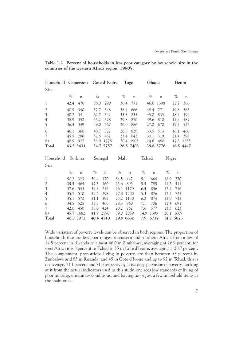
Table 1.2 Percent of households in less poor category by household size in thecountries of the western Africa region, 1990’s.

Household Cameroon Cote d’Ivoire Togo Ghana Benin

Size

% n % n % n % n % n

1 42.4 476 58.0 790 36.4 771 46.6 1398 22.7 366

2 40.9 340 57.7 548 38.4 666 48.4 771 19.8 3653 40.2 341 62.7 542 33.5 835 45.0 835 18.2 4944 38.9 352 55.2 578 29.8 870 39.6 810 17.2 5875 36.4 349 49.0 567 20.0 886 27.2 670 19.3 524

6 46.1 360 48.7 522 20.8 828 33.5 513 16.1 4607 45.5 286 52.5 432 23.4 642 30.1 319 21.4 3988+ 48.9 927 53.9 1778 20.4 1905 24.6 460 17.3 1255Total 43.5 3431 54.7 5757 26.5 7403 39.6 5776 18.5 4447

Household Burkina Senegal Mali Tchad Niger

Size

% n % n % n % n % n

1 50.2 323 59.4 170 34.5 447 5.1 664 18.9 2702 35.5 465 47.5 160 23.6 893 5.5 785 11.2 5113 37.6 545 39.8 216 26.1 1179 6.4 856 12.4 7164 35.7 510 39.6 298 27.8 1200 5.3 876 12.2 7225 35.1 572 31.1 392 25.2 1130 6.2 874 13.0 7336 34.5 525 33.5 460 28.3 960 7.1 706 11.4 6917 42.0 450 38.0 424 28.2 762 7.6 577 13.3 6238+ 45.7 1682 41.9 2590 39.0 2059 14.9 1399 20.1 1609Total 40.5 5072 40.4 4710 29.9 8630 7.9 6737 14.7 5875

Wide variation of poverty levels can be observed in both regions. The proportion ofhouseholds that are less poor ranges, in eastern and southern Africa, from a low of14.5 percent in Rwanda to almost 46.0 in Zimbabwe, averaging at 26.9 percent; forwest Africa it is 8 percent in Tchad to 55 in Cote d’Ivoire, averaging at 28.7 percent.The complement, proportions living in poverty, are then between 53 percent inZimbabwe and 85 in Rwanda, and 45 in Cote d’Ivoire and up to 92 in Tchad; this ison average, 73.1 percent and 71.3 respectively. It is a deep pervasion of poverty. Lookingat it from the actual indicators used in this study, one sees low standards of living ofpoor housing, unsanitary conditions, and having no or just a few household items asthe main ones.

7


16

Before observations on the pattern of poverty by household size is done there is needto control for intervening correlates of poverty. Three basic groupings emerge fromthese data, even without control for the intervening factors as can be observed inCharts in Appendix 2.

The first group is of countries which show the rising proportion of less poor withhigher household size: Zambia and Mozambique in eastern-southern Africa, and Tchadand Central African Republic (CAR) in the west. In contrast are those with a conversepattern of less poverty with smaller household size: Zimbabwe, Namibia, Kenya andComoros in eastern-southern Africa, and Ghana and Togo in the west. Most of theremaining countries (11) have mostly declining proportions of less poor, but risingnear the highest household size. Four of these however, have a U-shape: fluctuating atthe bottom over a distinct wide range of household size, 3 to 6; with Madagascar risinga bit then falling.

An additional variable ‘pattern’ is therefore created as per these groupings: that ofhigher proportions of less poor with higher household size.

Table 2.1 shows results of logistic regressions, showing odds of a household of a certainsize being in the poor category in contrast to the largest of size 8 persons and over,while controlling for correlates (intervening variables) of poverty. A value above 1.0indicates higher odds (in effect number of times) of being poor compared to thereference size. All odds are statistically significant at p < .01 or < .05 except whereindicated by a minus sign. For the controlled variables, with poverty category coded 0for less poverty and 1 for being poor, an odds value less than one means a higher valueof a variable is associated with less poverty.

It can be seen for both areas, first from the totals, that, now with control for othercorrelates, the pattern of less poverty with higher household size comes out clearly,and it is overwhelming as is shown by high statistical significance, mostly at less than.01 level (of error). For example in the eastern-southern Africa region the odds ofbeing poor decrease monotonically with higher household size: compared to largesthouseholds of eight members and above, a one-member household is nearly threetimes poorer, 2.3 times for the two-member, 1.7 for the three member, and so on;similarly in western Africa. Although not shown, within urban and rural areas ineach region this pattern holds. Thus almost all countries, except four (out of the ten)in eastern and southern Africa, and two (out of eleven) in western Africa, generallyshow this pattern. Even the exceptions, if not for not being significant statistically,show a tendency of the largest households as being less poor. However, two countriesin the western region, Ghana and Togo show the converse pattern: here smallerhouseholds show to be less poor than larger ones at high statistical significance (p <.01).

8


17

Table 2.1: O

dds ratios of a household of a certain size being poor compared to the largest by poverty/household size

pattern grouping in Eastern, Southern and W

estern Africa.

TO

TA

LZ

AM

BIA

UG

AN

DA

RW

AN

DA

KE

NY

AN

AM

IBIA

CO

MO

RO

SM

AD

AG

ASC

AR

WM

ZZ

NT

QZ

M

Household size / O

dds Ratios**

12.802

4.1492.102

7.5282.145

1.238-1.600-

2.480

22.334

3.1501.565

6.1611.883

1.327+1.525-

1.778+

31.704

2.2541.257+

4.4451.312+

.941-1.219-

1.189-

41.558

2.0191.265

3.1111.149-

1.040-1.051-

0.826-

51.576

1.5211.515

2.7331.489

1.143-1.123-

0.902-

61.322

1.4541.176-

2.0771.061-

1.099-1.358-

1.062-

71.178

1.143-1.063-

1.5951.158-

1.1190.882-

0.857-

8+ (R

ef.)1.000

1.0001.000

1.0001.000

1.0001.000

1.000Sex of head

0.870 0.892-

0.6731.358

0.923-1.082-

0.7170.962-

Age of head

0.9900 .989

0.9891.004

0.990 0.990

1.000+0.976

Location10.408

9.32711.034

7.7835.871

27.2894.362

29.093

Education of head0.811

0.8290.789

0.8010.817

0.8160.876

0.728

Prop. in labour force0.208

0.2500.323

0.0990.151

0.2850.477

1.112

Husb./w

ife pres.1.373

1.3411.157

1.5901.674

1.281854+

0.040-

Pattern1.211

--

--

1.534-

Sample

53,99815,692

14,858 5,955

8,130 9,363

Per caput GN

P,-

330310

230350

1,940400

250

026

022

012

)$ S

U( 8

991M

ZQ

=M

OZ

AM

BIQ

U, Z

MW

=Z

IMB

AB

WE

, TN

Z=

TA

NZ

AN

IA, M

GC

=M

AD

AG

ASC

AR

9


18

TO

TA

LT

CH

AD

MA

LI

CA

ME

RO

ON

GH

AN

AB

EN

INC

AR

NIG

ER

CO

TE

D’I

VT

OG

OB

UR

KIN

ASE

NE

GA

L

Hou

seho

ld s

ize

/ O

dds

Rad

io**

85.156.

51.287.2

45.799.1

1

77.195.

40.291.3

00.670.2

2

06.185.

94.174.2

04.427.1

363.1

46. 24.1

21.257.3

46.14

63.132.1

68.160.2

45.219.1

5

-42.1-29.

84.119.1

51.216.1

6

-89. -19.

+42.127.1

91.254.1

7

00.100.1

00.100.1

00.100.1

).feR(

+8

75. 75.

-68. 33.1

44.1-59.

daeh fo xeS

-99. 99.

-00.110.1

10.100.1

daeh fo egA

09.677.6

47.2181.8

76.4149.7

noitacoL Educ

atio

n of

hea

d.9

1 .

96 .

85 .

89 .

87 .

80

Prop

. in

labo

ur fo

rce

.47

.33

.49

.42

.57

.51

Hus

b./W

ife P

res.

.96-

1.00

.90

-1.

23 .

96-

1.10

--

--

--

22.nrettaP

833,4470,31

060,9631,91

879,11685,75

elpmaS Per

capu

t G

NP,

199

8 (U

S $)

-23

0 30

025

0 20

0 24

061

0 70

0 52

039

0 33

038

0

NB

: Dep

end.

var.:

pov

erty

cat

egor

y: L

ess p

oor=

0, P

oor=

1; S

ex: M

ale=

1, F

emal

e=2;

Edu

cati

on=

year

s att

ende

d sc

hool

; Loc

atio

n: U

rban

=1,

Rur

al=

2. H

USB

WIF

E (H

usba

nd a

nd W

ife p

rese

nt):

No=

0, Y

es=

1.

** A

ll si

gnifi

cant

at

p <

.01

leve

l, ex

cept

whe

re s

tate

d: +

Sig

nific

ant

at p

< .0

5; -

Not

sig

nific

ant.

10


19

Thus real groupings emerging are three, replacing earlier ones when no control forintervening factors was done. The first is of less poverty with higher household size,that is pervasive of the region; second is where this pattern is only a tendency, i.e. notsignificant; and third is where smaller households are less poor.

Important observations can also be made for the correlates of poverty, i.e. the variablesother than household size. All have the expected odds values, and importantly theyare statistically significant (mostly with p < .01) in all countries, confirming theirimportance as intervening factors of poverty. Thus less poverty is associated witholder age (a life cycle trend), though in eastern-southern Africa education also counts.Abject poverty conditions in rural areas can be observed clearly: over 10 times poorerthan urban areas. Notable is higher proportion of household members in labour forceat ages 15 years and over, where it is everywhere related to less poverty; together withhigher household size, these two are important explanatory variables of less povertyon which the focus is.

It is worth noting here that these findings do not by any means indicate that everyindividual big household is less poor than small ones or the converse. As can be seenin the bivariate case in Tables 1.1 and 1.2, one still observes high proportions in thepoor category at all levels of household size in all countries. It is a phenomenon thatneeds further study, but beyond the data available. However, this does not negatewhat the data and further analysis show: proportions of less poor significantly increasewith higher household size in most of Africa.

Supporting evidence can be drawn from the Egyptian and Turkish DHSs shown inTables 2.2 and 2.3 respectively. Contrasts of poverty in the Egyptian case rivals thoseof many other African countries.

The finding of less poverty with higher household size raises a lot of scepticism. It istherefore imperative to cast the methodology net wider for more information. Stepwiseregression is employed to see which factors are drawn into the equation, i.e. are moreassociated with poverty level. Here the number of factors are increased: those identifiedabove, and interaction among them (two-way interactions). This will be done watchingout for hypothesized factors: not only household size but its coming into the equationas per groupings of poverty/household pattern identified earlier.

Tables 3.1 and 3.2 show results of this stepwise logistic regression for the two regionsand country groupings observed.

11


20

Table 2.2: Egypt: logistic regression of poverty with household size (contrast withlargest), controlling for intervening variablesVariable (n) B S.E. Df Sign. R Exp (B)

(odds ratio)-4601.0000.7ezis dlohesuoH

1 ( 715) 1.6964 .1141 1 .0000 .1021 5.45452 (1247) .6854 .0825 1 .0000 .0565 1.98463 (1598) .6612 .0714 1 .0000 .0631 1.93724 (2155) .4181 .0626 1 .0000 .0450 1.51905 (2523) .3078 .0578 1 .0000 .0354 1.36046 (2125) .1841 .0590 1 .0018 .0192 1.20227 (1640) .1289 .0628 1 .0401 .0103 1.13768+ (Ref.) (3199) - - - - - 1.0000Sex of head -.0937 .0891 1 .2929 .0000 .9106Age of head -.0190 .0015 1 .0000 -.0855 .9812Location of house -.2709 .0369 1 .0000 -.0497 .7627Education of head -.0811 .0033 1 .0000 -.1685 .9221Prop. Labour force -1555 .0975 1 .1106 -.0051 .8560

Husb/Wife Present -.0703 .0797 1 3776 .0000 .9321

Table 2.3: Turkey: logistic regression of poverty with household size (contrastwith largest), controlling for intervening variablesVariable (n) B S.E. Df Sign. R Exp (B)


1 ( 335) 1.1622 .1141 1 .1706 3.19682 (1089) .5058 .0825 1 .0000 .0418 1.65823 (1218) .1765 .0714 1 .0000 .0074 1.19304 (1753) .1252 .0626 1 .1120 .0000 .88235 (1391) .2510 .0578 1 .2137 .0207 .77806 ( 881) .2783 .590 1 .0120 .0213 .75917 ( 575) .1440 .0628 1 .2307 .0000 .86598+ (Ref.) ( 843) - - - - - -Sex of head -.0935 .1331 1 .4826 .0000 .9108Age of head -.0058 .0023 1 .0103 .0220 1.0058Location of house -.0579 .0555 1 .0000 .0869 1.6106Education of head -.7004 .0080 1 .0000 -.0727 .9438Prop. Labour force -0681 .01585 1 .0000 -.0429 .4964Husb/Wife Present -.0703 .01163 1 05581 .0000 .9342

12


21

Table 3.1: Coefficients of stepwise multiple logistic regression of poverty categorywith household size, correlates and their interactions in the East and Southern andWestern Africa: total and rural/urban location

Coefficients**laruRnabrUlatoTacirfA nrehtuoS dna tsaE

HOUSEHOLD SIZE, PROP. LABOUR, PATTERN

Pattern (Poverty/Household size) .1884 .2468 -.1565

--9060. ezis dlohesuoH

4821.-4252.-9322.-ruobaL .porP ,ezis dlohesuoH

Household size, Husb./wife present -.0617 - -.0691

-3500.--daeh fo noitacude ,ezis dlohesuoH

1531.--5690.-noitacude ,ruobaLporP

-9413.-dlohesuoh fo daeh fo xes ,ruobaLporP

3600.---dlohesuoh fo daeh fo ega ,ruobaLporP

OTHER CO-RELATES

-4800.-6010.-)dlohesuoh fo daeh fo( egA

Education (of head of household) -.1033 -.2358 -.0628

--1041.2dlohesuoh fo noitacoL8230.--0330.-tneserp efiw/dnabsuh ,xeS

1010.---tneserp efiw/dnabsuh ,egA

+1320.---tneserp efiw/dnabsuh ,noitacudE

--3733. tneserp efiw/dnabsuh ,noitacoL

0852.10751. -tneserp efiw dna dnabsuH

Western Africa

2601. +0280. eziS dlohesuoH

7200.-1300.- egA ,eziS dlohesuoH

7140. noitacoL ,eziS dlohesuoH

2500.- 7600.- noitacudE ,eziS dlohesuoH

5141.- 3070.- ruobaLporP ,eziS dlohesuoH

Household Size, Husband/Wife Present -.0771 -.0491 -.0972111. 5603.- 4312. nrettaP

1110.1-3203.1-ruobaLporP

3675. noitacoL ,ruobaLporP

1550.-+5230.- 5340.- noitacudE ,ruobaLporP

7110.- egA ,ruobaLporP

2362.-xeS ,ruobaLporP

13


22

OTHER CORRELATES

9600. 3620. )dlohesuoh fo daeh fo( egA

9800.- noitacoL ,egA9100.-5100.- 7100.- noitacudE ,egA

1900. 2400. 4110. tneserp efiw/dnabsuH ,egA

1667,1noitacoL

1830.- noitacudE ,noitacoL

Location, Husband/Wife Present .3646

0121. 2021. daeH eht fo noitacudE

Education, Husband/wife Present .0404 .0598

7933.1-tneserP efiw/dnabsuH

8433. daeH fo xeS

6350.-3770.-3550.-noitacudE ,daeH fo xeS

4994.tneserP efiw/dnabsuH ,xeS

NOTES:1. ** All variables are significant at p < .01 level, except where stated.2. + Significant at p < .05.3. Coding:Dependent var: poverty category: Less poor=0, Poor=1;Sex (of Head): Male =1, Female =2;Education: years attended;Location of household): Urban =1, Rural =2;PropLabor: proportion of household members 15 years and above.4. Negative coefficient: The higher the value of a variable, or interaction, the less poor a

household is.

14


23

Table 3.2: C

oefficients (B) of stepw

ise multiple logistic regression of poverty category w

ith household size, correlatesand their interactions in the countries of E

ast and Southern Africa region

(a) Eastern and Southern A

frica

ZA

MB

IAT

AN

ZA

NIA

RW

AN

DA

KE

NY

AN

AM

IBIA

CO

MO

RO

MG

C

WM

ZA

DN

AG

UQ

ZM

Variables in he E

quation /

Coefficients**

HO

USEH

OLD

SIZE, PRO

P.

LAB

OU

R

Pattern (Poverty/Household size)

--

--

.4073

Household size, PropLabour

-.2279-.2041

-.2836-.1205

--

.688

Household Size, H

usb/wife pres.

-.0624-

-.1948H

ousehold Size, Age

--

.0051-

-.0007-

.010120.

-16

00.

--

4010

. no

itac

udE ,

eziS

dlo

hesu

oHH

ousehold Size, Location-

-.1108-.1108

--

--.130

PropLabour, Education-

--.2479

-.9114-.1143

- .175

PropLabour, Sex of Head

-.2596-.1815

--

--.329

-

PropLabour, Age

--

- .0265

-.0110

PropLabour, Location-

--

1.1121

OT

HER

CO

RR

ELAT

ES

Age (of head of household)

-.0129 .0175

- -.0317

Age, education of head

.0013+-

--

- -.792

-.003

-93

4.1

0923

,360

95,2

5457

.283

97.3

4129

.1no

itac

o L

4451

.--

-34

02.-

3523

.-no

itac

udE

15


24

Sex,

edu

cati

on-

--

-.060

1-

Sex,

Hus

band

/Wife

Pre

sent

.491

1-

--

.157

3Lo

cati

on, H

usba

nd/w

ife p

rese

nt-

- .7

151

.263

6 +6141. -

9452.--

noitacoL ,xeS Age

, Lo

cati

on-

-.018

4-.0

106

Educ

atio

n, L

ocat

ion

.057

8-.0

547

-.040

1-.0

456

MZ

Q=

MO

ZA

MB

IQU

E,

ZM

W=

ZIM

BA

BW

E,

MG

C=

MA

DA

GA

SCA

R

(b)

Wes

tern

Afr

ica

TC

HA

DM

AL

IC

AM

ER

OO

NB

EN

ING

HA

NA

CA

RN

IGE

RC

OT

E D

’IV

OR

ET

OG

O

BU

RK

INA

SEN

EG

AL

HO

USE

HO

LD S

IZE,

PR

OP.

LAB

OU

R

5342.+8321.

4773. ezis dlohesuo

H

4912.-3002.-

ruobaLporP ,ezis dlohesuoH H

ouse

hold

Siz

e, S

ex o

f hea

d-.0

574

-.213

7

16


25

9100

.-20

00.-

3400

.-eg

A ,ez

iS d

lohe

suo

HHousehold Size, H

usb./Wife Pres.

-.0965-.1530

3290

. 72

41.-

noit

acoL

,ez

iS d

lohe

suo

H

7310

.-+5

300.-

noit

acud

E ,ez

iS d

lohe

suo

H

6855

.2-

+493

9.-

ruob

aLpo

rP

2510

.

1320

.-eg

A ,ru

obaL

porPPropLabour, Sex

-.63274880

.-96

60.

noit

acud

E ,r

uoba

Lpor

P

5764

.76

96.

3347

. no

itac

oL ,r

uoba

Lpor

POT

HE

R C

OR

RE

LA

TE

S

Age, H

usband/wife present

.0114 .013178

30.

)dlo

hesu

oh f

o da

eh f

o( e

gA

3200

.-32

00.-

dae

H fo

noi

tacu

dE ,

egAA

ge, Location-.009419

01.-

8640

.-70

11.-

0990

.-da

eH f

o no

itac

udE ,

xeS

7855

.-23

13.1

1568

. da

eH f

o xe

SSex of Head, A

ge.010074

68.-

+674

3.-tn

eser

p efi

w/dn

absu

H ,da

eH f

o xe

SSex of head, Location-.2103

Education, of Head

.09584420

.-22

90.

tnes

erp

efiw/

dnab

suH ,

noit

acud

E

7712

. tn

eser

p efi

w/dn

absu

H

5269

.140

96.2

2522

.272

56.1

3746

.2no

itac

oL

4760

.-03

40.-

dae

H fo

noit

acud

E ,no

itac

oLLocation, Husband/w

ife present

17


26

A first important observation is that higher household size per se is in most countriesnot selected into the equation; where it is, as in Mali-Niger-Burkina, Ghana-Togoand Benin, it is related with higher poverty, as would be expected. A second importantobservation does not dismiss the argument of focus, of less poverty with higherhousehold size. Household size appears very much into the equations, but importantlywhen interacting with other variables. As can be seen with variables of householdsize or proportion in the labour force, almost all coefficients have a negative sign. Itshows therefore that higher household size, rarely per se, but mostly by interactionwith another variable is associated with less poverty. The more relevant and indeedimportant one is higher household size interacting with higher proportion of householdmembers being in the labour force ages of 15 years and above and found to be lesspoor.

Evidence from the Egyptian and Turkish DHSs show similar results.

2.1 Poverty by household structure

Table 4 shows odds ratios of poverty compared to a household with the highestproportion, i.e. .67 and higher, of its members in the labour force (ages of 15 years andabove), controlling for intervening factors of poverty including household size, forthe two African regions. Median age of the head of the household at each level is alsoshown in the right panel.

Table 4: Odds of being poor, and age of head of household by household’s proportionof members in the labour force ages of 15 and above in Eastern-Southern, andWestern Africa

(a) Eastern-Southern AfricaProportion in Odds of being poor* Median age of head

labour forceTotal Rural Urban Total Rural Urban

0 - .335 1.63 1.53 1.69 37.0 38.0 36.0.335 - .509 1.27 1.20 1.31 39.0 40.0 37.0.509 - .673 .99 .90 1.06 43.0 45.0 38.0.671 – 1.000 1.00 1.00 1.00 48.0 52.0 39.0

(b) Western Africa 0 - .335 1.7 1.4 2.1 40.0 40.0 39.0.335 - .509 1.4 1.2 1.5 42.0 43.0 40.0.509 - .671 1.2 1.2 1.3 45.0 46.0 43.0.671 – 1.000 1.0 1.0 1.0 44.0 50.0 39.0

*All odds significant at p < .001

18


27

Less poverty with higher proportions in the labour force can clearly be seen, as expectedfrom earlier results of logistic regression. Though not shown, this is true at disaggregatedlevel, whether by rural-urban location or grouping by pattern of poverty by householdsize. Over the life cycle, a household would be expected to have more of its membersolder, therefore in the labour force. It can be seen that the head’s age rises in proportionto members in the household, and given the earlier observation of less poverty relatedto higher size, it shows that a life cycle buildup of both wealth and size is shown toexist, importantly with a fair indication of causality (for wealth buildup) from labouravailability for both household production and in-coming income transfers.

The issue is examined further by looking at whether the correlates of poverty vary bypoverty/development level groupings above.

2.2 Correlates of poverty by development level

African countries were seen above to be in three groupings: the pervasive or dominantone of less poverty with higher household size, a second, where this pattern is notsignificant, and a third where smaller household were significantly less poor. Whetherthese are related to level of development is unclear. It is because this is notable only inEastern-Southern Africa. As shown in Table 2 (bottom), countries with the dominantpattern are less developed, with GNP per caput of US $ 210-350, while where thereis no significant pattern, i.e. in Namibia, Zimbabwe and the Comoros it is US $ 400-1,940 (Population Reference Bureau, 2000: 2-3). However in Western Africa, somecountries of the first, dominant group of less poverty with higher household size,namely Cameroon, Cote d’Ivoire and Senegal, show the highest income ($520-700)compared to Ghana and Togo, which though depicting a converse pattern of smallerhouseholds being less poor, are at incomes of only $330-390.

There seems to be an Eastern-South versus Western Africa contrast: developmentlevel in the former, and other factors, unknown in the latter. Some preliminaryindicators could be associated with modern or western life styles, probably highereducation, (e.g. Namibia and Ghana) rather than income that may be distinguishingthem from the dominant first group.

Tanzania is a relatively huge country, and is known to have wide variations indevelopment levels or modernisation. It is therefore disaggregated to see whether anypatterns emerge on the poverty/household size relationship.

2.3 Tanzania: poverty/household size pattern versus development

Regions of Tanzania fall into four main groups by pattern of poverty by householdsize. At one end is a dominant, first group, of less poverty with higher household sizein rural areas of most regions; at the other end is the converse, fourth group, with

19


28

lower poverty, smaller household in rural areas of some regions. In between the twoends are two groups, both in urban areas, one a complement of the first group butwhere the poverty/household size pattern is not significant and the second groupcontrasting with its rural, (fourth group) complement, where poverty is less with size.There is also another group not shown –the ‘outlier’ regions, namely Dodoma andSingida, that do not show any relationship with any of the factors being considered.Tables, 5.1 to 5.4 show logistic regression results of poverty level with household sizecontrolling for intervening variables for the four groups.

The first group shown in Table 5.1, is (a), the pattern of less poverty with higherhousehold size. As can be observed in the last column, the odds of a household of agiven size being poor compared to the largest, decrease with increase in householdsize. These are rural parts of most, 15 out of Tanzania’s 22 regions, accounting forover 81 per cent of the total sample households. These reflect the general countrywidepattern seen earlier and span basically the south, south-west, west and Lake (Victoria)areas of the country, and a few from the north-east. Most of these are the mainagricultural regions. This pattern is a highly significant one-to-one relationship. Thisis confirmed by stepwise logistic regression, panel (b) that brings in, at high significance(p < .0001), the interaction of higher household size with proportion of members inthe labour force.

Although attention is on the poverty pattern of household size, intervening variables,except one, have the right, expected (negative) signs, and are significantly associatedwith less poverty. However in rural areas of some regions the presence of both husbandand wife, i.e. a normal household is observed. The negative sign for sex of head inpanel (a) indicating unexpectedly less poverty for a household with a female head iseasily explained away by stepwise regression in panel (b), that it is less poor if thefemale head has higher education.

The second group, is the urban complement of the first group that includes mostregions, and Dar es Salaam City. It depicts a transition from the first, rural stage.Shown in Table 5.2 are results of stepwise regression to see which factors are ‘called’into the equation as significant in the level of poverty (the poverty pattern by householdsize however is only a tendency but not significant, therefore omitted).

The results show pretty much what is expected in urban areas: it is the interveningvariables of education per se, and its interaction with higher proportion of householdmembers being in labour force ages that are significantly related to less poverty(p < .0001). Additional significance is the head being female. Because Tanzania doesnot have a strong female economy as in Western Africa, being categorised as heads isnew. However, an emergent factor is that women work hard.

20


29

Table 5.1: Logistic regression of poverty with household size controlling forintervening variables: pattern of less poverty with higher household size in most ofrural Tanzania

(a) Contrast by household sizeVariable (n) B S.E. Df Sign. R Exp (B)


1 (265) 1.1866 .4079 1 .0036 .0556 3.2758

2 (453) 1.2003 .3194 1 .0002 .0761 3.3211

3 (541) .8231 .2567 1 .0013 .0629 2.2775

4 (604) .6437 .2282 1 .0048 .0534 1.9034

5 (611) .3798 .2105 1 .0712 .0245 1.4620

6 (539) .4404 .2260 1 .0514 .0293 1.5533

7 (428) .2341 2286 1 .3058 .0000 1.2637

8+ (Ref.) (680) - - - - - 1.000

Sex of head -.8752 .2421 1 .0003 -.0727 .4168

Age of head -.0112 .0051 1 .268 -.0373 .9889

Education of head -.2310 .0224 1 .0000 -.2229 .7937PropLabourForce -1.3090 .3827 1 .0006 -.0681 .2701

HusbWife Present -.2647 .2428 1 .2756 .0000 .7675

Stepwise regression

H/hold size, Prop. Labour Force -.2703 .0531 1 .0000 -.1068 .7631

Sex, Education of Head -.1071 .0224 1 .0000 -.0997 .8985

Age, Education of Head -.0018 .0007 1 .0049 -.0531 .9982

(REG = 1,2 RUR, n=4121 (81.14 %))

Coding: Poverty level: Poor=1, less poor=0

Sex of head: male=1, female=2

The third group, even though in urban location, presents a contrasting, indeedseemingly strange pattern relative to the first and shows that there is less poverty withhigher family size (Table 5.3). These are urban areas of Kilimanjaro, Zanzibar(excluding Pemba) and Morogoro regions. This difference is identified in the stepwiseregression results.

This sub-group eliminates both the seemingly strange less poverty/higher householdpattern, and shows the interaction of higher education level with higher proportionsof members being in the labour force. The size and labour force show socio-economicchanges from the typical state of higher household size cum higher proportion of

21


30

members in the labour force, seen for the majority of the regions. The second is theposition of females in bigger households and whether it is a female economy in urbanhouseholds.

Table 5.2: Results of stepwise logistic regression of poverty with household sizeand intervening variables in most urban areas of Tanzania (including Dar es SalaamCity)

N = 1428

RngiSfd.E.SBelbairaV Exp (B)

7537.353.-4630.17641.0703.-daeh fo xeS

Education of Head -.1448 .0318 1 .0000 -.0991 .8652

Education, PropLabourForce -.1464 .0394 1 .0002 -.0787 .8638

The fourth group, in Table 5.4, shows extremes of smaller households being less poor,in the rural location, as observed in the second urban group observed earlier. However,the pattern is not significant for the smallest households of 1 or two members, mostprobably due to the nature of the regions themselves: Kilimanjaro, Zanzibar, andMorogoro not predicting the full rural characteristics.

Table 5.3: Logistic regression of poverty with household size controlling forintervening variables: pattern of less poverty with higher household size in someregions of urban Tanzania

(a) Contrast by household size)B(pxERngiSfd.E.S)B()n(elbairaV

-4711.7210.3eziS dlohesuoH

3053.49501.051013406.2074.1)57(2-1

1809.21301.861.014644.5760.1)66(4-3

8365.34931.0300.15824.8072.1)46(6-5

0000.1-----)96().fer( +7

0384.8640.-4690.17734.7727.-daeh fo xeS4479.3680.-9130.11210.9520.-daeh fo egA

2197.9342.-0000.11940.2432.-noitacudE

PropLabourForce -2.4420 .9158 1 .0077 -.1209 .0870

HusbWifePresent -.1520 .4140 1 .7136 .0000 .8590

22


31

(b) Stepwise regression

N=274

0769.3731.-4300.14110.6330.-daeH fo egA

Household size, Sex of head -.0111 .0047 1 .0181 -.1012 .9890

Education, PropLabourForce -.3553 .0645 1 .0000 -.2848 .7010

Table 5.4: Logistic regression of poverty with household size controlling forintervening variables: pattern of less poverty with smaller household size in someregions of rural Tanzania

(a) Contrast by household size)B(pxERngiSfd.E.S)B()n(elbairaV

Household Size 3 .0469 .0438 -

3066. 0000.0362.18073.0514.-)732(2-1

8294. 6070.-7700.17562.7707.-)782(4-3

8195. 7740.-5730.12252.6425.-)192(6-5

7+ (Ref..) (251) - - - - - 1.0000

4854.6160.-3510.16123.9977.-daeh fo xeS6659.2902.-0000.15600.3440.-daeh fo egA

Education of head -.3135 .0334 1 .0000 -.2900 .7309

9249.0000.5209.10084.8850.-ecroFruobaLporP

HusbWifePresent -.1772 .3070 1 .5637 .0000 .8376

(b) Stepwise regression

N=1041

)B(pxERngiSfd.E.SBelbairaV

1889.7621.-0000.18200.0210.-daeh fo egA ,xeS

Education, Age of head -.0059 .0006 1 .0000 -.3030 .9941

Coding: Poverty level: Poor=1, less poor=0.

Sex of head: male=1, female=2.

23


32

These results show households headed by older females, or any headed by an olderperson with higher education, to be less poor. It is both a life cycle build up of wealthand perhaps emergence of a female economy.

The general observation is that less poverty with higher household size is pervasive inmost of west, central and south Tanzania, especially the agricultural regions knownfor less economic diversification. This is in contrast to urban centres and parts of thenorth-east where the pattern is not significant or is the converse. It is a clear changeof pattern of development as earlier noted in the eastern-southern Africa region.

3.0 Discussion

The pattern of less poverty with household size is pervasive of the African region,with indications of changes with modernisation being clear in eastern-southern Africabut more complex in the west. The most pertinent issue of the study is how this canbe interpreted; and the implications, particularly on population policy and developmentinter-relationships.

The pattern seems to reflect more of older household heads, over the life cycle, havingaccumulated both more children and wealth. Relevant to this study is that the basis ishigher household size from which both a higher proportion and number of workers isdrawn, which augers well with the labour shortages that micro level farm studies haveshown as characteristic of the labour-intensive smallholder agriculture which is thebasis of the African economy (Ruthenberg, ed., 1968; Cleave, 1974; Kamuzora, 1980).The observed high fertility behaviour in Africa completes the circuit.

What are the implications for the family planning movement? It suggests that peopleshould be left to decide and be helped to have the number of children that theydesire, which is a UN convention assuming, as homines sapientes et economici, thatpeople know what is best for themselves. The latter has all along been put loud andclear by people themselves: they use family planning methods mainly for spacing(Bongaarts, 1991; Cohen, 2000), and attempt to limit fertility only at high parities, asreported from e.g. African country DHSs, like the Tanzania Demographic and HealthSurvey 1996 (Tanzania, 1997: 45-50). Thus efforts by the family planning movementfor young households to stop at just a few children may be misguided. Concentrationshould be on reproductive health in general, and specifically child spacing for healthychildren, and let couples decide themselves on the number.

The findings of this study satisfy both theory and reality and that in contrast to thealternative, less poverty in smaller households, that were argued above, and seem tobe wanting in both methods and data.

The findings of this study also bring attention to the protracted debate on therelationship between population growth and development, as there is little evidenceof negative effects. It is a phenomenon that has been observed right from Kuznets by

24


33

1965 through to his student Easterlin (1967). Of perhaps more significance, giventhe power-politics of the debate, are three high powered studies, two, 15 years apart,1971 and 1986 sponsored by the (American) National Academy of Sciences andNational Research Council and the third one - the World Bank’s 1984 WorldDevelopment Report where consultants saw no evidence of deleterious effects exceptagreeing that “on balance” lower population growth was preferred (see reviews inPopulation and Development Review 1985, 1986 respectively), but it did not amusethe 1986 study lead consultants (Simon, 1986). These studies in effect repudiate theCoale-Hoover thesis, fertility decline, the prime prescription of Coale and Hoover(1958).

The thesis might trigger population ageing with its negative consequences that currentdeveloped countries and Asia dread and actually fear in terms of the burden of care ofan increasing proportion of the elderly by decreasing proportions of the workingpopulations (see e.g. Ratnasabapathy (1994); JOICFP News, 1991, 1998). The highlyunlikely reversal of the trend by a rise in fertility, leads to the disliked but inevitableoption of immigration of dissimilar racial stock. Further, the thesis negates implicationsof findings of this study, less poverty with higher household size connected to laboursupply in a labour demanding socio-economy of Africa.

The Boserup (1965) thesis of the positive power of population growth, which is arguedby Simon (1981, 1996) and succinctly evaluated by Julian Simon (RIP, 1998) isexplained by Ahlburg (1998).

25

…. Economics does not conclusively show that a greater number ofpeople implies slower economic development or a lower standard ofliving. … Julian Simon made a valuable contribution to thepopulation growth debate. He forced us to think harder about theissues and to consider the long-run positive consequences ofpopulation growth as well as the short-run negative impacts. …(ibid.: 324).

(emphasis in original)

4.0 Areas for further research

Although a pattern of less poverty has with no doubt been established, yet at eachlevel of household size there are high proportions in the poverty category conflictingwith the pattern; e.g. poor at high household size and the converse. There is needtherefore to investigate factors behind this phenomenon. For example aspects onpoor household management where data is not available could be the crucial factor.


34

References

African Academy of Sciences, 1994: “Statement by the African Academy of Sciencesat the Population Summit” Population and Development Review 20 (1): 238-9.

Ahlburgh, Dennis A., 1998: ‘Julian Simon and the population growth debate.’Population and Development Review 24 (2):317-328.

Bagachwa, M.S.D. (ed.), 1994: Poverty Alleviation in Tanzania: Recent ResearchIssues. (Dar es Salaam: Dar es Salaam University Press, 1994).

Bongaarts, John, 1991: ‘The KAP-gap and the unmet need for contraception.’Population and Development Review 17 (2): 293-313.

Boserup, Ester, 1965: The Conditions of Agricultural Growth (London: Allen andUnwin).

Boserup, Ester, 1981: Population and Technological Change: A study of long-termtrends. (Chicago University Press).

Cleave, J.H., 1874: African Farmers: Labour Use in the Development of SmallholderAgriculture (New York: Praeger Publishers).

Cohen, Barney, 2000: ‘Family planning programs, socio-economic characteristics, andcontraceptive use in Malawi.’ World Development 28 (5): 843-60.

Easterlin, Richard A., 1967: ‘The effects of population growth on the economicdevelopment of developing countries.’ The Annals of the American Academy ofPolitical and Social Sciences 369: 98-108.

Easterlin, Richard A., 1985: ‘Review Symposium’ Population and DevelopmentReview: 11 (1): 113-38

Kamuzora, C.L., 1980: “Constraints to labour time availability in African smallholderagriculture: the case of Bukoba District, Tanzania”. Development and Change 11(1), 1980.

Kamuzora, C.L., (in press): A Youth-full Population: the ultimate resource for Africa,Tanzania (Dar es Salaam University Press) (earlier presented as Professorial InauguralLecture, 25 October, 1999, University of Dar es Salaam)

Kamuzora, C.L. and S. Gwalema, 1998: Aggravation of Poverty in Rural Bukoba26


35

District, Tanzania: Labour Constraints, Population Dynamics and the AIDS Epidemic.Research Report No. 98.4. (Dar es Salaam: REPOA).

Kamuzora, C.L. and William Mkanta, 2001: Poverty and family size in Tanzania:multiple responses to population pressure? Research Report N0. 2001.4(Dar es Salaam:REPOA).

Lee, Ronald, 1985: ‘Review Symposium’ Population and Development Review 11(1): 113-38.

McNicoll, G., 1995: “On population growth and revisionism: further questions.”Population and Development Review 21 (2): 307-40.

Mosk, Carl, 1992: Review of Robert Hodge and Naohiro Ogawa, 1991. Populationand Development Review 18 (2): 365-67.

Mtatifikolo, F., 1990: Resources for Human Development: Tanzania. Report toUNFPA. (Dar es Salaam: UNFPA).

Mwisomba, S.T. and B.H.R. Kiilu, 2001: “Demographic factors, householdcomposition, employment and household welfare.” Paper No. EM5 of REPOA 6th

research Workshop, Dar es Salaam, April 18-19, 2001 (Dar es Salaam: REPOA).

Population Reference Bureau, 2000: 2000 World Population Data Sheet (WashingtonDC: PRB)

Ruthenberg, H., 1968: “Some characteristics of smallholder farming in Tanzania”, inH. Ruthenberg (ed.).

Ruthenberg, H., 1968: Smallholder Farming and Smallholder Development inTanzania (London: C. Hurst and Co.).

Semboja, J., 1994: “Poverty assessment in Tanzania: theoretical, conceptual andmethodological issues.: in Bagachwa (ed.): 31-56.

Sender, J. and S. Smith, 1990: Poverty, Class and Gender in Rural Africa: A TanzanianCase Study. (London: Routledge).

Simon, Julian L., 1981: The Ultimate Resource (Princeton University Press)

Simon, Julian L., 1996: The Ultimate Resource II (Princeton University Press).

27


36

Tanzania, 1997: Demographic and Health Survey, 1996 (Dar es Salaam and CalvertonMD USA: Bureau of Statistics and Macro International).

Appendix 1 Construction of a possessions index

The construction of a possessions index goes in the following manner. A type of anitem is given a weight or score: the value of the weight/score given is determined byan item’s relative standing on level of value. For example a sewing machine is certainlymore valuable and shows one having more wealth than a table or chair; so would bea motor vehicle compared to the sewing machine. Simply an arithmetic sum of theweights would give the possessions index: a higher weight value indicates more wealth.There are however important refinements that need consideration for a more properindex.

The value of the weight could be a score, e.g. 1,2,3,…., with any interval. This leavesroom for arbitrariness and important attention paid to the differences in the valuesbetween items. A hierarchical ‘binary system’ is preferred as shown in the example.On the survey questionnaire, a household has (=1) or does not (=0) possess an item.With an item’s relative standing as an indicator of level of wealth an item is given aposition as shown in the following example. Take the above items, namely chairs,tables, sewing machines and a car, valued higher in this order by taking positions one,two to four respectively. With two persons, one possessing chairs, tables and a car; theother person possessing chairs and a sewing machine. Their possessions indexes wouldbe as follows:

Chairs Tables Sewing Car POSSESSIONS

Machine INDEX

Person No 1 1 1 0 1 1011

Person No 2 1 0 1 0 101

Note: The last position on the index is the position of lowest value.

Person No. 1 is certainly wealthier than No. 2. Their possessions indexes are respectively1011 and 101. (The arithmetic of combining a person’s items can easily be discerned.)The advantage here is that, knowing an items position, one can tell what particularitems a person possesses.

Grouping can be done into manageable ‘Possessions classes’: in this study the classes(they are actually a step to arriving at a poverty category) are poorest, poor and lesspoor. It can be noted that the word rich is avoided because as will be seen in theresults one is dealing with largely poverty conditions in the survey area.

28


3729

The items going into the possessions index (with their value position in that order asexplained above) are: motor car/lorry, motor cycle, sewing machine, bicycle, radio,lantern, tables, chairs, cattle, and sheep/goats; an additional item going into the indexis housing quality (materials making the roof, walls and floor, and number of rooms,where the latter is converted into a crowding variable of number of persons per room.

The three ‘Possessions classes’ (Posclass) are then as follows:

1. POOREST: owning a bicycle OR radio and any of the lower value items (includingnone);

2. POOR: owning a radio and a bicycle and any of the lower items;

3. LESS POOR: owning a sewing machine OR any of higher, and lower value items.

Housing quality (materials it is made of) was also determined with higher value put tothe roof, then walls, and lastly the floor. A qualification was made by adding a crowding(persons per room) dimension. In the TDHS data, further poverty variables, namelytype of water source and toilet exist, were used. Three classes of quality were arrivedat: poor housing (basically a thatched roof), improved housing (corrugated iron roofbut basically with mud walls and floor), and modern (corrugated iron /tile roof andbrick/stone/cement walls and floor).

By combining housing quality and possessions class a two ‘Poverty Categories’(PAUPE4) was produced to facilitate logistic regression analysis.


3830

Ch

art 2

Per

cen

t Ho

use

ho

lds

Les

s P

oo

r

010203040506070

12

34

56

78

Ho

use

ho

ld S

ize

Percent Less Poor

Tanz

ania

Uga

nda

B

enin

Cot

e d'

Ivoi

reC

amer

oon

Sen

egal

Rw

anda

Mal

iN

iger

Bur

kina

Mad

agas

car


3931

Ch

art 1

Pe

rce

nt H

ou

se

ho

lds

Le

ss

po

or b

y S

ize

0

10

20

30

40

50

60

70

12

34

56

78

Ho

use

ho

ld S

ize

P e rc e n t L e ss P o o

Za

mb

iaM

oz

am

biq

ue

Tc

ha

d C

AR

Zim

ba

bw

eN

am

ibia

Ke

ny

aC

om

oro

sG

ha

na

To

go


40

REPOA RESEARCH REPORTS

REPOA Research Report 97.1: “Poverty and the Environment: The Case of InformalSand-mining, Quarrying and Lime-Making Activities in Dar es Salaam, Tanzania”(by G. Jambiya, K. Kulindwa and H. Sosovele)

REPOA Research Report 97.2: “The Impact of Technology on Poverty Alleviation:The Case of Artisanal Mining in Tanzania” (by W. Mutagwaba, R. Mwaipopo-Ako andA. Mlaki)

REPOA Research Report 97.3: Educational Background, Training and TheirInfluence on Female-Operated Informal Sector Enterprises (by J. O’Riordan, F. Swaiand A. Rugumyamheto)

REPOA Research Report 98.1: The Role of Informal and Semi-formal Finance inPoverty Alleviation in Tanzania: Results of a Field Study in Two Regions (by A.K.Kashuliza, J.P. Hella, F.T. Magayane and Z.S.K. Mvena)

REPOA Research Report 98.2: Poverty and Diffusion of Technological Innovationsto Rural Women: The Role of Entrepreneurship (by B.D. Diyamett, R.S. Mabala andR. Mandara)

REPOA Research Report 98.3: The Use of Labour-Intensive Irrigation Technologiesin Alleviating Poverty in Majengo, Mbeya Rural District (by J. Shitundu and N.Luvanga)

REPOA Research Report 98.4: Labour Constraints, Population Dynamics and theAIDS Epidemic: The Case of Rural Bukoba District, Tanzania (by C.L. Kamuzora andS. Gwalema)

REPOA Research Report 98.5: Youth Migration and Poverty Alleviation: A CaseStudy of Petty Traders (Wamachinga) in Dar es Salaam (by A.J. Liviga and R.D.K.Mekacha)

32


41

REPOA Research Report 99.1: Credit Schemes and Women’s Empowerment forPoverty Alleviation: The Case of Tanga Region, Tanzania (by I.A.M. Makombe, E.I.Temba and A.R.M. Kihombo)

REPOA Research Report 00.1: Foreign Aid, Grassroots Participation and PovertyAlleviation in Tanzania: The HESAWA Fiasco (by S. Rugumamu)

REPOA Research Report 00.2: Poverty, Environment and Livelihood Along theGradients of the Usambaras in Tanzania (by Adolfo Mascarenhas)

REPOA Research Report 00.3: Survival and Accumulation Strategies at the Rural-Urban Interface: A Study of Ifakara Town, Tanzania (by Anthony Chamwali)

REPOA Research Report 00.4: Poverty and Family Size in Tanzania: MultipleResponses to Population Pressure? (by C.L. Kamuzora and W. Mkanta)

REPOA Research Report 00.5: Conservation and Poverty: The Case of AmaniNature Reserve (by George Jambiya and Hussein Sosovele)

REPOA Research Report 01.1: Improving Farm Management Skills for PovertyAlleviation: The Case of Njombe District” (by Aida Isinika and Ntengua Mdoe)

REPOA Research Report 01.2: The Role of Traditional Irrigation Systems(Vinyungu) in Alleviating Poverty in Iringa Rural District (by Tenge Mkavidanda andAbiud Kaswamila)

33


42

OTHER PUBLICATIONS BY REPOA

BOOK

Poverty Alleviation in Tanzania: Recent Research Issues. Dar es Salaam: Dar es SalaamUniversity Press (Edited by M.S.D. Bagachwa)

SPECIAL PAPERS

REPOA Special Paper 1: Changing Perceptions of Poverty and the EmergingResearch Issues (by M.S.D. Bagachwa)

REPOA Special Paper 2: Poverty Assessment in Tanzania: Theoretical, Conceptualand Methodological Issues (by J. Semboja)

REPOA Special Paper 3: Who’s Poor in Tanzania? A Review of Recent PovertyResearch” (by Brian Cooksey)

REPOA Special Paper 4: Implications of Public Policies on Poverty and PovertyAlleviation: The Case of Tanzania (by Fidelis Mtatifikolo)

REPOA Special Paper 5: Environmental Issues and Poverty Alleviation in Tanzania(by Adolfo Mascarenhas)

REPOA Special Paper 6: The Use of Technology in Alleviating Poverty in Tanzania(by A.S. Chungu and G.R.R. Mandara)

REPOA Special Paper 7: Gender and Poverty Alleviation in Tanzania: Issues fromand for Research (by Patricia Mbughuni)

REPOA Special Paper 8: Social and Cultural Factors Influencing Poverty inTanzania (by C.K. Omari)

REPOA Special Paper 9: Guidelines for Preparing and Assessing REPOA ResearchProposals (by REPOA Secretariat and Brian Cooksey)

REPOA Special Paper 10: An Inventory of Potential Researchers and Institutionsof Relevance to Research on Poverty in Tanzania (by A.F.Lwaitama)

REPOA Special Paper 11: A Bibliography on Poverty in Tanzania (by B. Mutagwaba)

34


43

REPOA Special Paper 12: Some Practical Research Guidelines (by Brian Cookseyand Alfred Lokuji)

REPOA Special Paper 13: Capacity Building for Research (by M.S.D. Bagachwa)

REPOA Special Paper 14: Guidelines for Monitoring and Evaluation of REPOAActivities (by A. Chungu and S. Muller-Maige)

35

POVERTY AND FAMILY SIZE PATTERNS: Comparison - Repoa

Documents

Transcript of POVERTY AND FAMILY SIZE PATTERNS: Comparison - Repoa