Poverty Alleviation and Child Labor

By ERIC V. EDMONDS AND NORBERT SCHADY*

Forthcoming in American Economic Journal: Economic Policy

Final version: September 2011

Poor women with children in Ecuador were selected at random for a cash transfer

equivalent to 7 percent of monthly expenditures. The transfer is greater than the

increase in schooling costs at the end of primary school, but it is less than 20

percent of median child labor earnings in the labor market. Poor families with

children in school at the time of the award use the extra income to postpone the

child's entry into the labor force. Students in families induced to take-up the cash

transfer by the experiment reduce their involvement in paid employment by 78

percent and unpaid economic activity inside their home by 32 percent. These

declines in economic activity are accompanied by an increase in time in unpaid

household services, but overall time spent working declines.

* Edmonds: Department of Economics, Dartmouth College, 6106 Rockefeller Hall, Hanover NH 03755 USA (email: eedmonds@dartmouth.edu);

Schady: Inter-American Development Bank, 1300 New York Avenue, NW, Washington DC 20577 USA (email: norberts@iadb.org). The views

in this paper do not necessarily reflect those of the Inter-American Development Bank, its Executive Directors, or the countries they represent.

We appreciate the helpful comments of Caridad Araujo, Kathleen Beegle, Milo Bianchi, Francisco Ferreira, John Giles, Sylvie Lambert, Marco

Manacorda, David McKenzie, Christopher Snyder, Zafiris Tzannatos, and especially Hilary Hoynes and our referees, as well as seminar

participants at Cornell, Georgetown, Maryland, Paris School of Economics, Ohio State, University of California at Davis, and Vanderbilt and

conference participants at the IZA/World Bank Employment in Development Conference, Juan Carlos III / UCW Conference on the Transition

from School to Work, NBER Summer Institute, and NEUDC. We thank Isabel Beltran, Ryan Booth, and Jennifer Chong for help preparing the

data.

1

More than one in five children in the world work. Most of these working children live in poor

countries. This paper is concerned with the relationship between current family economic status

and child labor in poor countries. There are two distinct strands of research. The first considers

whether working while young influences a household's current economic status through the

economic contribution of children (Manacorda 2006), and the impact of child labor on local

labor markets (Basu and Van 1998). The second examines whether current economic status

influences the decision to send children to work. Understanding economic influences on child

time allocation is important for the political economy of child labor regulation and the design of

child labor policy (Doepke and Zilibotti 2005). This second strand of research is the focus of this

paper, which examines child time allocation responses to experimental variation in a cash

transfer program in Ecuador.

In the recent literature on child labor responses to variation in economic status, reviewed in the

next section, there is a debate on the extent to which child time allocation responds to income

among poor households. There are many theoretical reasons why poverty may cause child labor.

However, the time allocation of children and household incomes are joint outcomes of a single

decision-making process, so establishing a causal relationship is difficult. Many correlates of

family income influence the economic structure of the household, raising omitted variables

concerns.

This study considers how child time allocation in Ecuador responds to receipt of the Bono de

Desarrollo Humano (BDH) cash transfer. The evaluation of the BDH randomly assigned

eligibility for the cash transfer to some poor households and not to others. The BDH transfer is

$15 per household per month, 7 percent of monthly expenditures for recipient households. The

amount does not vary across eligible families. The transfer is paid to mothers, and does not have

any conditions attached. We use the random assignment from the evaluation of the BDH as our

source of variation in economic status.

We show that $15 a month given as the BDH reduces child labor. These results are consistent

with a growing literature that documents that cash and in-kind transfers can reduce child work,

but are novel in several ways. First, the BDH results in reductions in all kinds of work, including

paid employment. The declines in paid employment are large, and are concentrated among

children who were students at the time of random assignment. Lottery-induced take-up of the

BDH is associated with a 41 percent decline in paid employment for the full sample, and a 78

2

percent decline for children who were students at baseline. The focus on paid employment is

novel because earlier research has largely focused on unpaid economic activity in the family

farm or business.

Second, households in the present study were not given a strong financial incentive to send

children to school. This distinguishes our findings from those based on PROGRESA in Mexico

and other conditional cash transfer programs, where the structure of the transfer changes the

relative cost of schooling. The government of Ecuador carried out a social marketing campaign

that stressed the importance of investments in human capital at the time the BDH was launched,

but there was no attempt to enforce schooling attendance or other actions related to human

capital. Some families in our data mistakenly report that they are supposed to send their children

to school as a condition to receive the transfer. Schady and Araujo (2008) document that the

change in schooling in the treated population is largest among these families. However, as we

discuss below, it does not appear that the declines in paid employment we observe are a result of

a misunderstanding of the requirements of the BDH.

Third, child labor declines with the BDH even though the size of the transfer is less than

foregone child labor earnings. Fewer than 2 percent of children in paid employment report

earning less than $15 a month and median earnings are $80 per child per month. We argue that

the rigidities in hours in paid employment and in the length of the school day explain why paid

employment declines despite the fact that the transfer does not cover foregone earnings. The

transfer may push the optimal child labor supply for poor families to below that necessary to

participate in paid employment. In fact, we observe that among the poorest students, there

appears to be some movement from paid employment into unpaid, household based economic

activity for fewer hours.

The rest of the paper proceeds as follows. Section I reviews the existing evidence on the

income elasticity of child labor. The BDH program is described in section II, and BDH's impact

on child labor is presented in section III. Section IV concludes with a discussion of the

interpretation of our findings as well as its implications for future research on child labor.

I. Existing Evidence on Child Labor and Living Standards

An estimated 306 million children are economically active in the world (ILO 2010). These

children are overwhelmingly in poor countries, and cross-country differences in GDP per capita

3

alone can explain two-thirds of the cross-country variation in economic activity rates (Edmonds

2010). Perhaps the most researched question in the empirical child labor literature is whether

there is a causal relationship between some measure of living standards and the time allocation

of children. Many studies document that children are less likely to work in richer households and

that children work less as a household gets richer. 1 This finding is not universal.2 Several

studies document important confounding factors that are correlated with both living standards

and time allocation.3 Attributing causation is difficult because child time allocation and

economic status are joint outcomes of a single decision-making process.

There are several reasons why children might work more in poorer settings. We have in mind a

single household decision-maker deriving utility from consumption today and the child’s future

well-being (produced by investing in child schooling today). This agent maximizes utility by

allocating child time between schooling, paid employment and work inside the household,

subject to a time and cash constraint. Schooling and paid employment are both difficult to do

part-time. There are fixed costs associated with searching for and traveling to paid employment,

and the formal labor market production technology may require coordination with other workers.

Work inside the home is more flexible. Schooling is also inflexible, because it is difficult to

make adequate school progress with sporadic attendance and awkward to leave after a few hours.

As a result, it is rare to combine paid employment with schooling. Combining unpaid household

based work with schooling is more feasible.

Preferences cause schooling to increase with income. Because of the rigidity in time in paid

employment, a rise in demand for schooling reduces participation in paid employment as income

rises holding wages constant. As time shifts from paid employment to school, work inside the

household may rise as that’s presumed to be more flexible. An emphasis on agent preferences as

a key determinant of paid employment and child labor is commonplace, even in models without

explicitly emphasizing schooling. Rosenzweig and Evenson (1977) put preferences for leisure in

1

The following rely on cross-sectional variation: Behrman and Knowles 1999; De Carvalho Filho 2008; Chiwaula 2010; Cogneau and Jedwab 2008; Dammert 2006; Dammert 2008; Edmonds 2006; Edmonds, Pavcnik, and Topalova 2010; Wahba 2006. Studies using panel data include: Beegle, Dehejia, and Gatti 2006; Dillon 2008; Duryea, Lam, and Levison 2007; Edmonds 2005; Edmonds and Pavcnik 2005; Glewwe and Jacoby 2004; Jacoby and Skoufias 1997; Yang 2008.

2 The following are a list of published studies that do not find support for a negative correlation between living standards and economic

activity: Bhalotra and Heady 2003; Dumas 2007; Ersado 2005; Kambhampati and Rajan 2006; Psacharopoulos 1997; Ray 2000; Swaminathan 1998.

3 There is a wide array of confounding factors documented in the literature. For examples, see: Basu, Das and Dutta 2007; Fafchamps and

Wahba 2006; Kruger 2007; Manacorda and Rosati 2010; Mueller 1984; Rosenzweig and Evenson 1977; Schady 2004.

4

the utility function. Basu and Van (1998) is built on a luxury axiom that posits that children work

only when the agent cannot otherwise overcome subsistence needs.

Liquidity constraints are implicit within our framework. They plan an important role in many

models of child labor supply (e.g. Baland and Robinson 2000, Ranjan 2001) and their

importance in child labor decisions has some empirical support (Edmonds 2006). Even if

schooling were purely an investment, liquidity constraints can generate a link between income

and child labor if liquidity constraints force families to choose less school than optimal given the

market return and opportunity costs to schooling.

There are other reasons why increases in income could result in declines in child labor.

Increases in income, including cash transfer income, could reduce the need for child labor for

household self-insurance (Beegle, Dehejia, and Gatti 2006; de Janvry et al. 2005). Food,

nutrition, books, pencils, notebooks, and transportation all might become more available with

increases in income, and could increase the relative return to time in school. Higher income can

affect changes in productivity in household based work. For example, income may induce

families to specialize more, as the quality of products purchased in market may dominate the

quality of products manufactured at home (Edmonds and Pavcnik 2006). That is, higher income

may induce a decline in productivity in home production with implications for paid employment

and schooling. Alternatively, additional income could increase productivity inside the household

if it facilitates the accumulation of working capital that is complementary to child labor (Basu,

Das, and Dutta 2010). The result might be less paid employment but more employment within

the household.

There is considerable heterogeneity in how researchers define child labor in these studies

(Edmonds 2008 is a review). Evidence on the link between paid employment and living

standards is especially elusive. Paid employment is rare among children. Edmonds and Pavcnik

(2005b) document that 1 out of 42 children between the ages of 5 and 14 in the 36 countries

covered by the UNICEF MICS2 project work for pay. The fact that paid employment is rare and

the joint determination of living standards and paid employment combine to create complicated

econometric problems that make elusive compelling evidence on an income elasticity of paid

employment. Studies of large-scale conditional cash transfer programs (CCTs) such as Mexico's

PROGRESA sometimes find an impact of CCTs on paid employment (for example, Schultz

2004). However, CCTs change both the standard of living and the relative return to schooling.

5

Researchers since the origins of the human capital literature (e.g. Schultz 1960) have emphasized

the primary importance of relative returns to education in time allocation decisions. Hence,

without further assumptions, the CCT evidence is ultimately not informative about the

relationship between living standards and paid employment.

II. Background on BDH and Its Evaluation

Ecuador has had a cash transfer program, the Bono Solidario, since 1998. Recipient

households received $15 per month per family without conditions attached. Bono Solidario was

meant to assist poor families during an economic crisis. It continued past the economic crisis and

was poorly targeted. BDH replaced Bono Solidario beginning in mid-2003. A key difference

between BDH and Bono Solidario is that initial eligibility for the BDH is explicitly means-tested

based on a census conducted in 2001.4 Only the poorest two quintiles of the population are

eligible to receive the BDH's $15 per month.

In transitioning Bono Solidario to BDH, the government launched a social marketing

campaign that stressed the importance of the BDH in supporting the human capital of poor

children. The government paid for radio and newspaper advertisements emphasizing this. Local

leaders were supposed to hold town-hall style meetings to explain the purpose of the BDH. Like

the Bono Solidario program it replaced, BDH transfers have never been made explicitly

conditional on specific investments in child human capital (for example, school enrollment). The

government of Ecuador felt it did not have the technical capacity to monitor compliance with any

such conditions.

Incorporation of new households, those who had not received the Bono Solidario previously,

worked as follows. Program officials in local BDH offices were given a list of eligible recipients

by the central government based on their scores on the means test. Local BDH officials then

informed those who were eligible. To actually receive benefits, those who were told they were

eligible had to visit in person any branch office of the largest network of private banks (Banred)

or the National Development Bank (Banco Nacional de Fomento) on prearranged days, or

arrange for monthly electronic transfers to accounts in their name. Benefit distribution started in

the latter half of 2003, without commitments on the length of benefits or when eligibility would

4

Starting in 2001, the government developed a family means test, called the Selben index. The Selben index was computed by first conducting a census of household assets, then using principal component analysis to create a single asset index.

6

be reassessed. There was no on-going means test in the program, so recipients did not need to do

anything to establish on-going eligibility after they had been informed of their eligibility in 2003

based on the 2001 data collection. Eligibility was not reassessed between 2003 and 2008.

The rollout of BDH explicitly contained a randomized component in 4 of Ecuador's 24

provinces. Within provinces selected for the evaluation, parishes were randomly drawn. A parish

is unit of local government with an average population of 26,503. Within selected parishes, a

sample of 1,488 households was randomly selected into the evaluation. There were three filters

for incorporation into the evaluation sample. First, households had to be BDH-eligible. Second,

households that already received Bono Solidario transfers, and continued to be eligible for the

BDH program, were excluded from the evaluation—for these households there was no policy

change, and therefore nothing to evaluate. Third, households had to have at least one child age 6-

17 at the time the means test data was collected.

Households in the evaluation sample were randomly assigned to a “treatment” group (lottery

winners) and a “control” group (lottery losers) with a random number sorter. On average, there

are 14 lottery winners age 11-16 at baseline and 13 lottery losers per evaluation parish.5 Lottery

winners would immediately be activated for transfers. Lottery losers were excluded for the

duration of the program. In most parishes, there are more BDH-eligible households than those

who were selected into the evaluation using the lottery. The process of informing eligible

individuals and initiating the transfers did not differ in evaluation and non-evaluation parishes.

Within evaluation parishes, it did not differ between lottery winners and other BDH-eligible

households. Households, including those in the evaluation sample, were not told their scores on

the means test. It would be difficult for an individual to assess their own eligibility ex-ante as

eligibility was based on the national distribution of wealth, not local, and because the weights

given to different components of the proxy means were not revealed. For this reason, it would

also be difficult for households to manipulate their scores on the proxy means test to ensure

eligibility.6 Lottery losers were not informed that they were on the original list or that they had

been removed from that list. A reasonable presumption is therefore that lottery losers assumed

5

The poorest two-fifths of the population is eligible for the BDH. This does not correspond to two-fifths of each parish as living standards are not uniformly distributed, and the study areas are slightly wealthier than average in Ecuador (see the On-Line Appendix 1). The 27 study subjects per parish reflects the fact that the evaluation excluded subjects receiving Bono Solidario in the past and that our focus is primarily on the population age 11-16.

6 See Camacho and Conover (2011) for evidence of widespread manipulation of a similar poverty index in Colombia, but only after the

algorithm used to calculate the score had been made public.

7

that they were, in fact, ineligible for transfers. An important feature of this experiment is that,

unlike the PROGRESA evaluation, randomization took place at the household level, rather than

the community level. Within a parish, we observe both lottery winners and losers.7

The main sources of data used in this paper are the baseline and follow-up surveys designed

for the BDH evaluation. Both surveys were carried out by the Catholic University of Ecuador, an

organization that had no association with the BDH program and no responsibility for its

implementation or evaluation. The baseline survey was collected between June and August 2003.

The follow-up survey was collected between January and March 2005, after BDH recipients had

been receiving transfers for more than a year. The survey instrument includes a roster of

household members, basic socio-demographic characteristics of these members, detailed time

allocation and schooling information for school-age children, employment status for adults,

dwelling characteristics, household asset holdings, and an extensive module on household

expenditures, following the structure of the 1998–99 Encuesta de Condiciones de Vida (ECV).

We aggregate expenditures, including consumption of home-produced items into a consumption

aggregate, appropriately deflated with regional prices of a basket of food items collected with the

surveys.

Attrition between baseline and follow-up does not appear to be a substantive issue for our

analysis. 94.1 percent of households were re-interviewed. Among households that attrited, most

had moved and could not be found (4.2 percent); in a few cases no qualified respondent was

available for the follow-up survey despite repeat visits by the enumerator (1.0 percent), or the

respondent refused to participate in the survey (0.5 percent). Attrited children were less likely to

be enrolled in school at baseline. They were older. There is no relation between assignment to

the study groups and attrition. Baseline differences between attrited and other households in per

capita expenditures, assets, and maternal education are small and insignificant.8

Our analysis focuses on comparing lottery winners to lottery losers. This is not equivalent to

comparing BDH recipients to non-recipients as there was considerable non-compliance with the

7

For additional information on the BDH and how the evaluation population differs from the rest of Ecuador, see the On-Line Appendix 1. 8

In a regression of a dummy variable for attrited households on a dummy variable for lottery winners, with standard errors corrected for within-parish correlation, the coefficient is 0.054, with a robust standard error of 0.057. In a simple regression of baseline enrollment on a dummy variable for attrited households, the coefficient is –0.083, with a robust standard error of 0.038. When a set of unrestricted child age dummies is included in the regression, the coefficient on the dummy variable for attrited children becomes insignificant: The coefficient is –0.033, with a robust standard error of 0.034. On the other hand, a joint test shows that the age dummies are clearly significant (p value of less than 0.001). The attrition rate for children 10 to 16 at baseline was similar to the household rate: 93.9 percent of children 10-16 interviewed at baseline were recaptured at follow-up.

8

experiment. 38 percent of children 11-16 at baseline in households that lost the BDH lottery

received transfers. None should. 69 percent of children 11-16 in households that won the lottery

took up the BDH. Despite non-compliance with the experimental design, winning the lottery

increases the probability a child lives in a household receiving the BDH by 82 percent. The On-

Line Appendix 2 compares the characteristics of BDH recipients that won the lottery and those

that did not. The differences in observables between these two groups are not statistically

significant individually or jointly.9 Even so, there may be differences in unobservables, perhaps

including a higher degree of “pushiness” among lottery losers who nevertheless received

transfers. Because the results we present instrument BDH take-up with the lottery assignment, as

discussed in greater detail below, they are relevant for children whose likelihood of receiving

transfers was affected by the lottery. If treatment effects are heterogeneous, our estimates may

not apply to other BDH-eligible households.

The lottery appears to have been successful in attaining balanced treatment and control

samples. Schady and Araujo (2008) establish the validity of the randomization for children 5-16.

Our key results are for children 11-16 at baseline, and we therefore focus our discussion on the

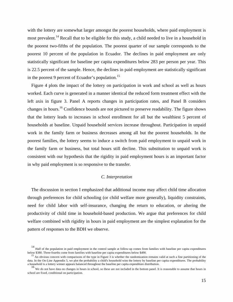
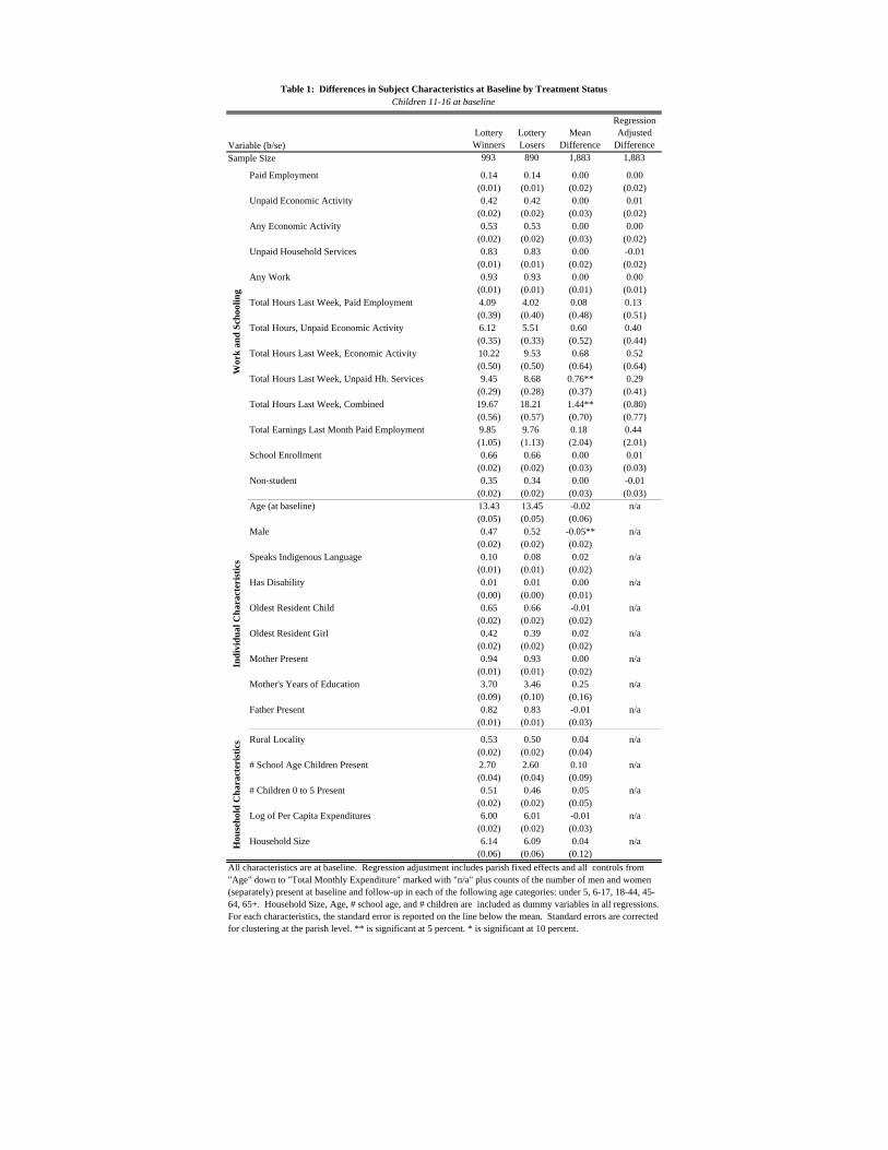
validity of the randomization for children 11-16. Table 1 summarizes background characteristics

of children and their families for the 1,883 children age 11 and older at baseline, separately for

lottery winners and losers.10 The top panel of table 1 summarizes work and schooling activities at

baseline. Children can participate in multiple categories of work. Paid employment occurs

outside of the child’s home, while unpaid economic activity is work in the family farm or

business. 42 percent of children are engaged in unpaid economic activity at baseline. Together,

unpaid economic activity plus paid employment are defined as economic activity in this study.

53 percent of the sample is economically active at baseline. Unpaid household services include

chores such as shopping, cleaning, and caretaking. The category “any work” combines economic

activity and unpaid household services. The total hours and earnings statistics include non-

participants in the activity coded as zeros. Children in paid employment work substantially more

hours than do children in unpaid economic activity or unpaid household services. This can be

seen in Table 1 by scaling up the hours by participation rates, which are three times larger in

9

The F-statistic associated with the null that the mean differences in baseline characteristics reported in the On-Line Appendix 2 are jointly zero is 0.86 with a P-value of 0.67.

10 Our analysis focuses on children above age 10 at baseline. Follow-up is on average 1.5 years pass the baseline, and school drop-out rates

start to increase from age 12.

9

unpaid economic activity than in paid employment, and six times larger in unpaid household

services. Conditional on participating, average hours in paid employment is 40 hours per week.

The last two rows of the work and schooling panel report information on schooling.

Enrollment refers to the current school year at time of interview. Children can be enrolled and

yet be coded as non-students. A non-student is either not enrolled in the current school year, or is

enrolled but reports having quit or stopped attending for reasons other than teacher strikes or

personal illness. At baseline, one-third of non-students work for pay, 44 percent work in unpaid

economic activity, and 75 percent participate in unpaid household services. Two percent of

subjects report being idle at baseline, where idle is defined as being a non-student who does not

engage in any work. We do not discuss these idle children further. We do not see movements in

idle status with the lottery, but we do not have power to measure small changes in the prevalence

of idleness.

Most of the background characteristics in table 1 appear similar, but gender and total hours in

unpaid household services (and thus combined hours) are not balanced between lottery winners

and losers. Column 3 of table 1 reports the raw mean difference between columns 1 and 2 as well

as whether the difference is significantly different from zero at 10 or 5 percent. The F-Statistic

associated with a test of the hypothesis that the differences are jointly zero is 1.37, with a p-value

of 0.11.

Girls spend a third more time in unpaid household services than do boys conditional on

participating, and 60 percent more when non-participants are included (girls have higher

participation rates). The differences in hours in unpaid household services (and total combined

hours) between lottery winners and losers are related to the differences in gender composition

between the two groups. The final column of table 1 mimics the empirical specification used

throughout this study. It considers whether the differences in work and schooling between lottery

winners and losers persist after including the controls used in all later tables. Specifically, the

reported regression-adjusted difference is the coefficient on an indicator that the child’s family

won the BDH lottery obtained from a regression of the row variable (the dependent variable) on

this lottery indicator, all of the controls listed in the table from age down, parish fixed effects,

and the household composition controls listed in the note to the table. The difference in total

hours worked in unpaid household services and the difference in total hours combined are not

significant with regression adjustment. Gender appears to be the key characteristic that is

10

responsible for the significant mean difference in hours worked—controlling for gender alone is

enough to fail to reject the null that there is no difference between treatment and control

populations in any of the variables for hours worked. The lack of balance in gender does not

appear substantive in our analysis as we can never reject the null hypothesis that boys and girls

are affected equally by the program.11

Several other studies have considered the impact of BDH transfers: Paxson and Schady (2010)

show that transfers improve the health and development of preschool-aged children, and Schady

and Rosero (2008) show that a higher fraction of transfer income is used on food than is the case

with other sources of income. Most directly related to this paper, Schady and Araujo (2008)

show that the program has large effects on school enrollment rates. Though the transfers are

small, the impact they have on children seems to be large.

III. Main Findings

The BDH lottery is independent of employment opportunities and the household's time

allocation decision-making process. Hence, the lottery solves the problem of confounding factors

and simultaneity that plague most of the literature on the impact of poverty on child labor. As

discussed in section I, there are good theoretical reasons to expect that the transfer would result

in declines in economic activity rates and paid employment.

Our empirical strategy is straightforward. The randomization was stratified by parish, so we

include parish fixed effects throughout, , and cluster robust standard errors by parish. With the

inclusion of parish fixed effects, our empirical approach only captures effects of the BDH that

are net of any spillovers to the control population. We control for the vector of baseline time

allocation characteristics listed in table 1, , as well as the other child and household level

characteristics listed in table 1, .12 Age, household size, number of children 0-5, and number

of school-age children are recoded as dummy variables throughout the empirical work and

denoted .

11

In an earlier version of this paper, we bifurcated the sample by gender and by urban-rural. Boys and girls appear to react to the lottery similarly, meaning we could not reject the null that changes in time allocation with the lottery were the same for boys and girls. We also found similar responses to the lottery in rural and urban areas. Although the magnitudes of the results were slightly larger in rural areas, the urban - rural differences were not statistically significant.

12 The only controls included not listed in Table 1 are counts of the number of household members by age and gender present at baseline and

follow-up. These are not included in Table 1, because they would add an additional page in length to the Table.

c

0i

0iX

a

11

Our reduced form results consider the impact of winning the BDH lottery. We regress a child

labor indicator for child i in parish c at follow-up (denoted as time period 1) on the controls

above and an indicator for whether the child’s family won the BDH lottery, :

(1)

is an error term that is 0 in expectation conditional on the other controls listed in equation (1).

The reduced form mimics the actual policy implementation of providing lists of BDH-eligible

recipients to localities. The impact of being on the list will be different from the impact of

receiving transfers because of imperfect compliance. To estimate the impact of lottery-induced

BDH receipt, we replace in equation (1) with an indicator for whether the family receives the

BDH, and instrument for non-random receipt of the BDH with .

Our study focuses on children age 11-16 at baseline, and some of the results we report below

break down the sample between children who were students at baseline, and those who were not.

For both groups, the lottery increases take-up by 33 percentage points. 2SLS results will be

equivalent to multiplying the reduced form by 3.03 for both subgroups. The substantive

assumption in interpreting this rescaling as the impact of the BDH for households whose

likelihood of receiving the BDH was affected by the lottery is that the act of appearing on the

BDH-eligible list (winning the lottery) had no effect on child labor decisions beyond its effect on

take-up.

We use the 2SLS results to compute a counterfactual mean for non-receipt of the BDH. We

cannot use the mean of the dependent variable at follow-up in the control because of

contamination of the experimental design. Instead, the counterfactual mean is the predicted value

of the second-stage regression for the treated population with the BDH indicator set to zero. The

counterfactual means for most forms of work will be greater than the baseline means from table

1, because at follow-up study subjects are 1.5 years older on average. Dividing the estimated

impact of the BDH by the counterfactual mean is not the average percentage impact of the BDH,

but it is useful as a way of interpreting the magnitude of the estimated impact.

1icH

il

1 0 0ic c a i i r i icH X l

ic

il

il

12

A. Overall results

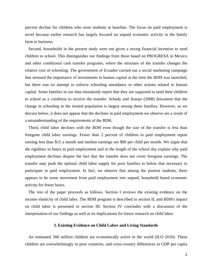
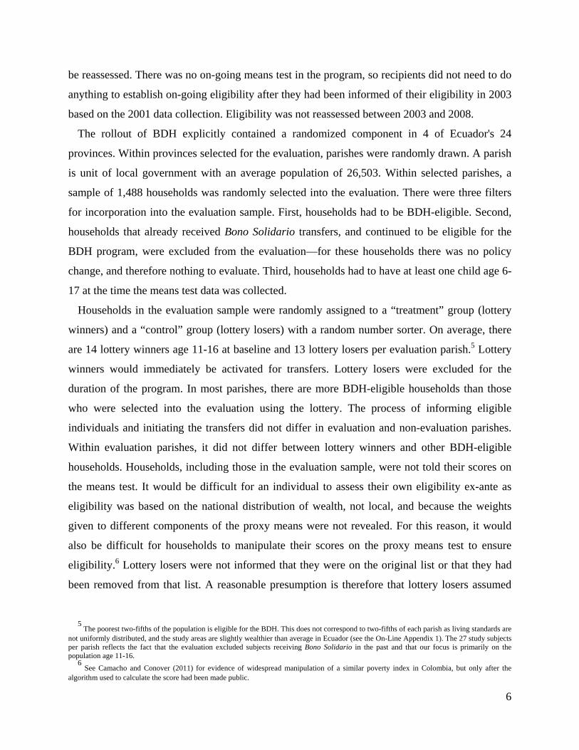
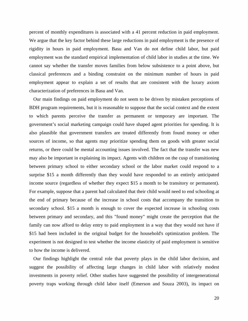
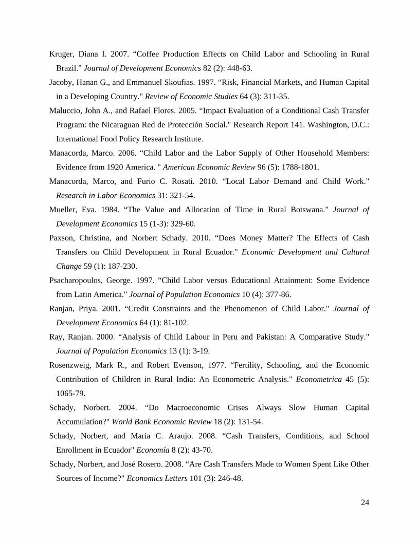
Children in low-income households in Ecuador participate in different activities by age. Figure

1 plots participation rates at baseline in paid employment, unpaid economic activity, unpaid

household services, and school enrollment against age at baseline for the pooled samples of

lottery winners and losers. Participation in paid employment is extremely unusual before age 12.

In contrast, child participation rates in unpaid economic activity and unpaid household services

are similar for ages 8 through 16. Because the main focus of this paper is on the effect of cash

transfers on paid employment, the estimates we report below are limited to children age 11-16 at

baseline (and thereby 12 -17 at follow-up). Results for children ages 5-10 and all ages pooled are

in the On-Line Appendix 3.

Our first set of results is reported in Table 2. The first row of Table 2 contains the first stage

results alluded to above. Subsequently, each cell in columns 1 and 2 of table 2 is from a different

regression. Each row indicates the dependent variable. The first column reports the reduced-form

effect of the lottery on the row variable. The second column reports the 2SLS estimate of the

effect of lottery-induced take-up of the BDH on the row variable. The third column reports the

predicted value of the second stage regression for the treated population in the absence of BDH

receipt.

The lottery reduces paid employment of children by 3.2 percentage points. The 2SLS results

show declines in paid employment of 9.9 percentage points. Relative to the counterfactual

participation rate of 24.3 percent, this implies a 41 percent reduction in paid employment.

Unpaid economic activity declines by 19 percentage points. Relative to the counterfactual

participation rate of 55.1 percent, this implies a 34 percent reduction in unpaid economic

activity.

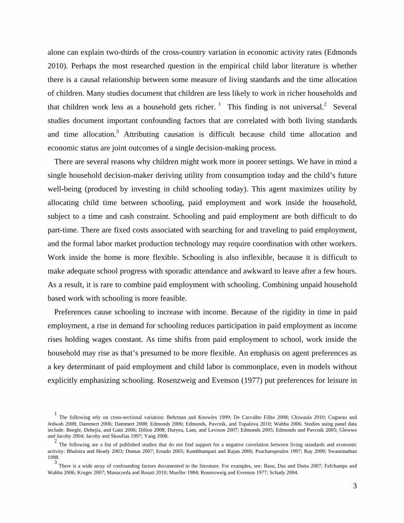
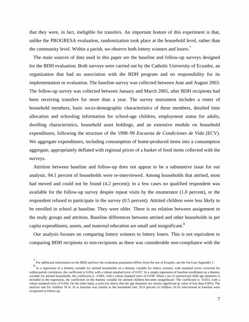
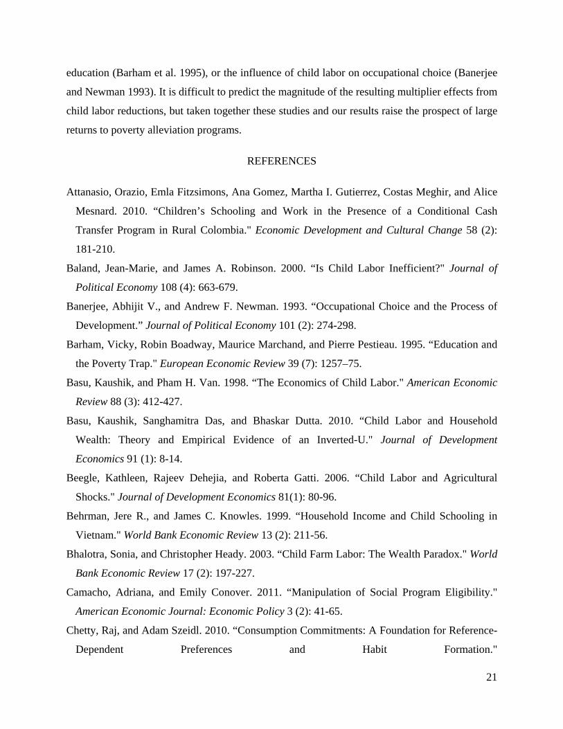
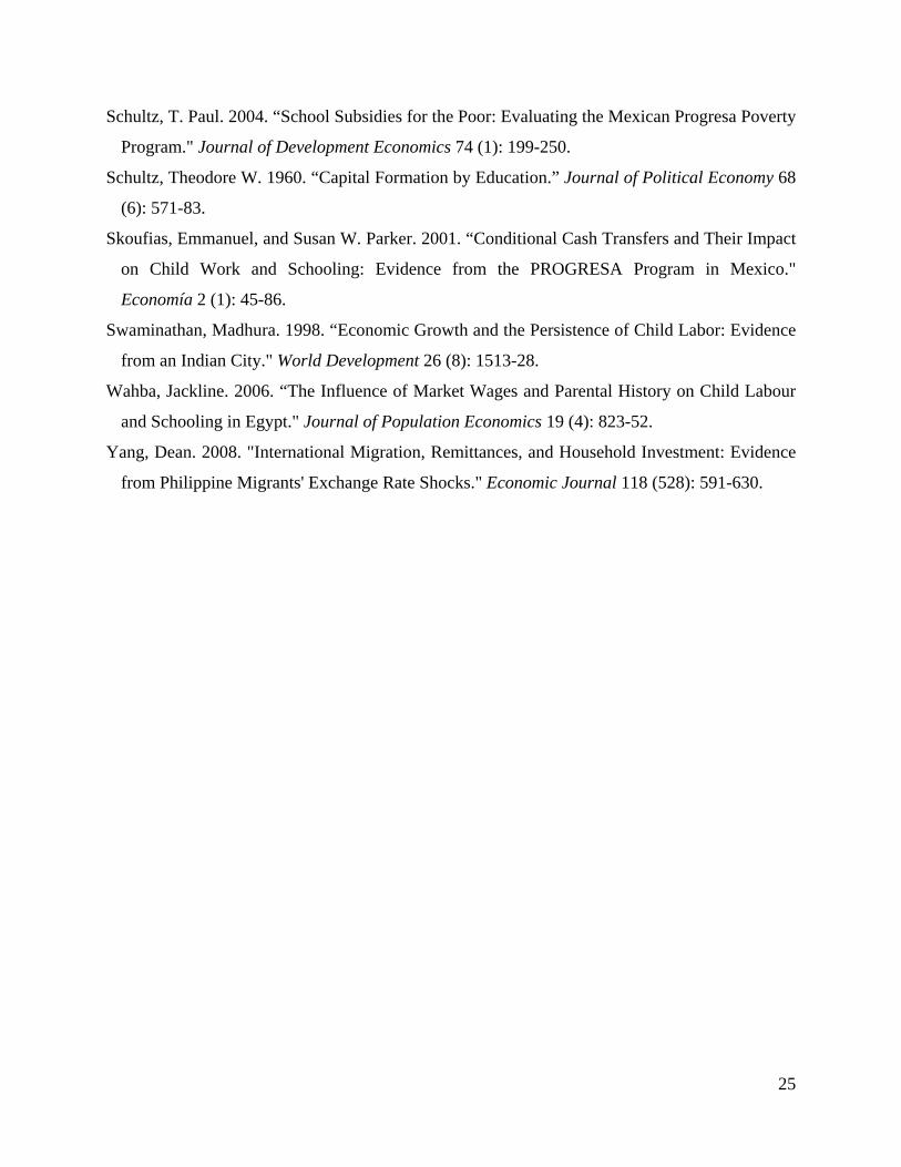
The change in paid employment appears to be driven mainly by changes in the extensive

margin (participation), rather than the intensive margin (hours). The total hours worked in paid

employment, conditional on working, is 40 hours. If that average were to stay fixed, a 9.9

percentage point reduction in participation implies reduction of 4.0 hours in paid employment. In

practice, we observe 2.7 fewer hours worked in paid employment. The fact that the decline in

paid employment is largely in the extensive margin is consistent with the strong concentration of

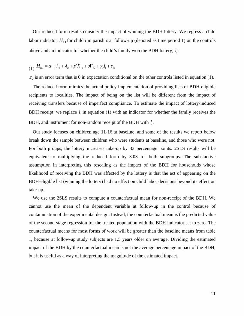
hours worked in paid employment around 40 hours per week. Figure Two is a histogram of total

hours worked in paid employment in the last seven days at follow-up for lottery losers (the

13

control sample). The mode, median, and mean hours worked in paid employment is 40 hours per

week. Where we see other minor spikes (5-10 hours, 20-24 hours, 45-50 hours) tends to be at

multiples of 8 hours, consistent with hypothesis that there is some inflexibility in hours worked

in paid employment within the day. The fact that the mass is so concentrated at 40 hours per

week implies that most who work in paid employment do so full time.

There is some evidence that the decline in paid employment is at the lower part of the earning

distribution. In table 2, the decline in participation in paid employment that results from the BDH

implies a decline of earnings of $8.3 per month, but we observe an actual decline in earnings of

only $1.8 per month. Given that most of the adjustment in paid employment is in the extensive

margin, this smaller decline in earnings implies that those who stop paid employment with the

transfer earn less than average.

B.Heterogeneity

This rigidity in paid employment makes it difficult to combine paid employment with

schooling. In our data, fewer than 1 in 7 children in paid employment at baseline were enrolled

in school. In contrast, out of every 20 children in unpaid economic activity at baseline, 13 were

enrolled in school. If there are fixed costs of re-entry, those who are out of school and in paid

employment at baseline are apt to stay out of school in the future. In fact, we observe in the

control group that less than 1 in 10 children out of school and in paid employment had re-

enrolled in school by follow up.

We consider whether the effect of the lottery and BDH varies with the child’s student status at

baseline with the hypothesis that non-students are unlikely to be affected by lottery-induced take-

up of BDH. Non-students are less apt to be affected, because reenrollment is rare (our definition

of non-student excludes transitory absences for health or teacher strikes). There may be fixed

costs to re-entering school, the experience of contributing economically to the household may

change perceptions of basic needs or reference income (as in Koszegi and Rabin 2006), or there

may durable consumption plans that are difficult to reverse (Chetty and Szeidl 2010). To allow

for heterogeneity with student status, we estimate equation (1), including an interaction of the

lottery winning dummy with an indicator that the child was not a student at baseline. The results

of this modification to our reduced form are in columns 1 and 2 of table 3. Column 1 contains the

14

reduced form effect of winning the lottery on the row variable for students.13 The effect of

winning the lottery for non-students is the sum of column 1 and 2. The 2SLS results in columns

3 and 4 instrument for the BDH indicator and its interaction with the non-student at baseline

indicator using the lottery dummy and its interaction with the non-student at baseline dummy.

The counterfactuals in columns 5 and 6 are the predicted values of the 2SLS for students and

non-students respectively after constraining the BDH dummy and its interactions to be zero.

Table 3 shows that the declines in paid employment are entirely concentrated in children who

were students at baseline. The 2SLS estimates indicate that, among baseline students, there was a

decline of 15 percentage points in paid employment as a result of the BDH, which is equivalent

to 78 percent of the counterfactual mean. Among non-students, there is essentially no decline in

paid employment associated with receipt of the BDH. In contrast, the decline in unpaid economic

activity associated with the BDH is larger among non-students than students. For non-students

(but not students) there is also a small decline in household chores. The BDH also results in

larger increases in school enrollment among baseline students than non-students. It makes sense

that patterns in school enrollment more closely mirror paid employment than unpaid economic

activity, as paid employment tends to be for more hours and may lack the flexibility in hours that

would make combining with schooling feasible.

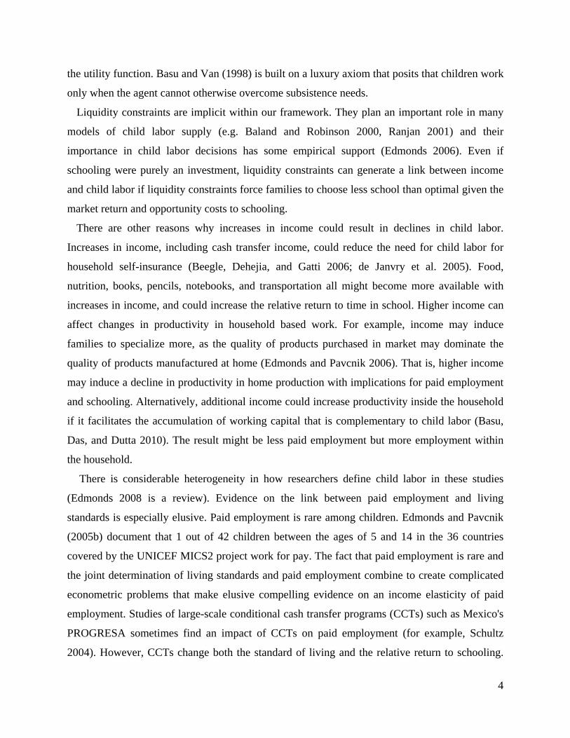
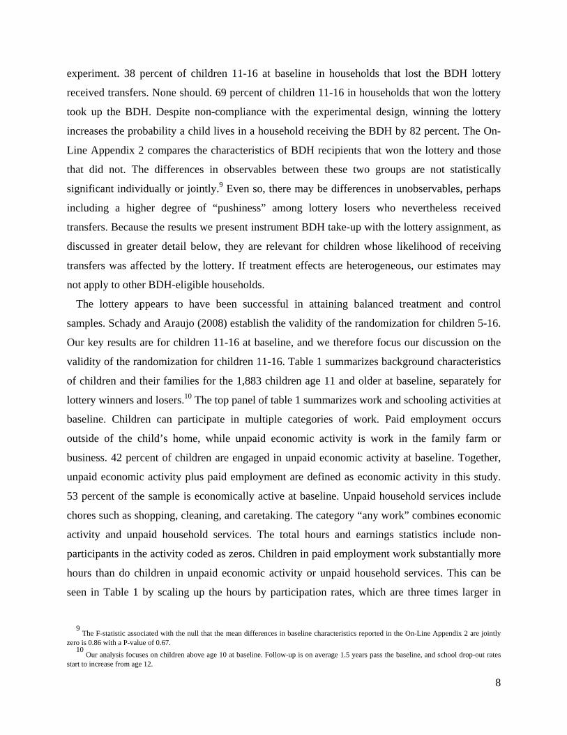
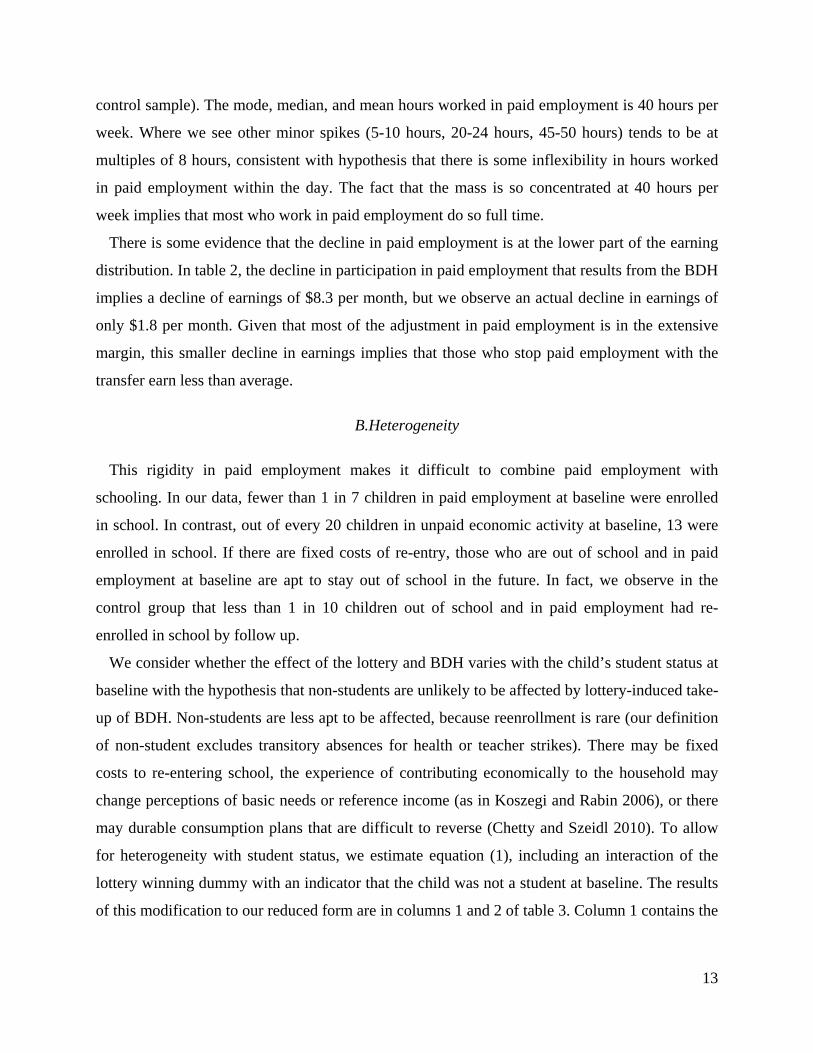
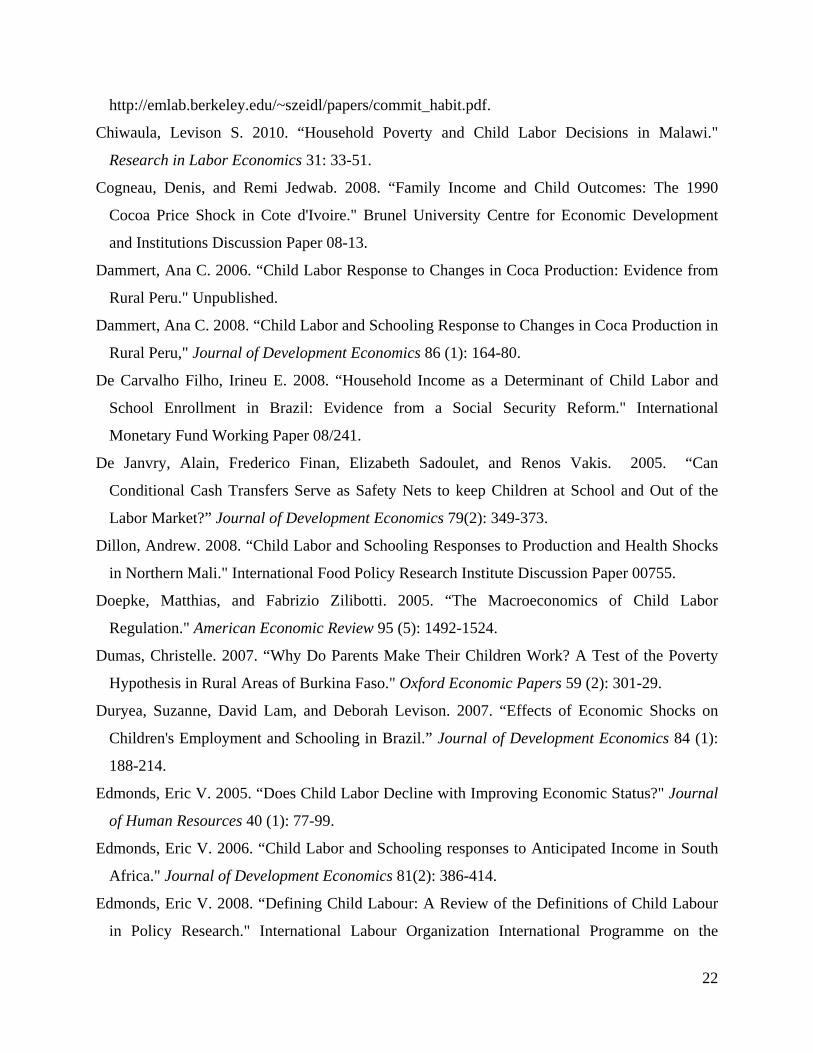
The effects of lottery-induced BDH receipt on paid employment are concentrated in students.

It is logical to suppose that its effects should be largest in poorer families where paid

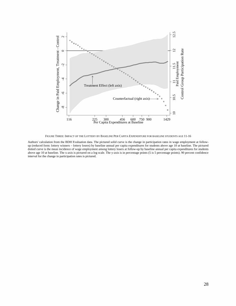
employment is most prevalent. We consider this in Figure 3. The sample is limited to students

age 11-16 at baseline. We measure living standards with baseline per capita expenditures. Figure

3 contains two local-linear regressions. On the left axis, we plot the reduced form effect of the

lottery on participation in paid employment in the last 7 days by baseline per capita expenditures.

Specifically, the left axis is the change in participation rates in paid employment at follow-up

(lottery winners – lottery losers). We also picture 90 percent confidence intervals around this

reduced form treatment effect. On the right axis, we plot the participation rate in paid

employment for the control sample by baseline per capita expenditures. This is the counterfactual

for the lottery treatment. The figure suggests that the declines in paid employment associated

13

On-Line Appendix 4 explores the validity of the randomization among baseline students. There are more females and more rural subjects among lottery winners. These are important controls in examining the effect of the lottery within students. The F-Statistic associated with the hypothesis that the differences between lottery winners and losers are jointly zero among students is 2.12 with a P-Value of 0.02 because of these two characteristics. For non-students, the F-Statistic for this test is 0.74 with a P-Value of 0.82.

15

with the lottery are somewhat larger amongst the poorest households, where paid employment is

most prevalent.14 Recall that to be eligible for this study, a child needed to live in a household in

the poorest two-fifths of the population. The poorest quarter of our sample corresponds to the

poorest 10 percent of the population in Ecuador. The declines in paid employment are only

statistically significant for baseline per capita expenditures below 283 per person per year. This

is 22.5 percent of the sample. Hence, the declines in paid employment are statistically significant

in the poorest 9 percent of Ecuador’s population.15

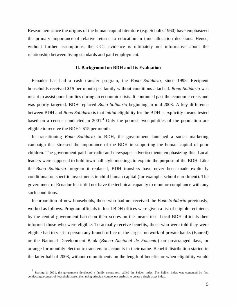
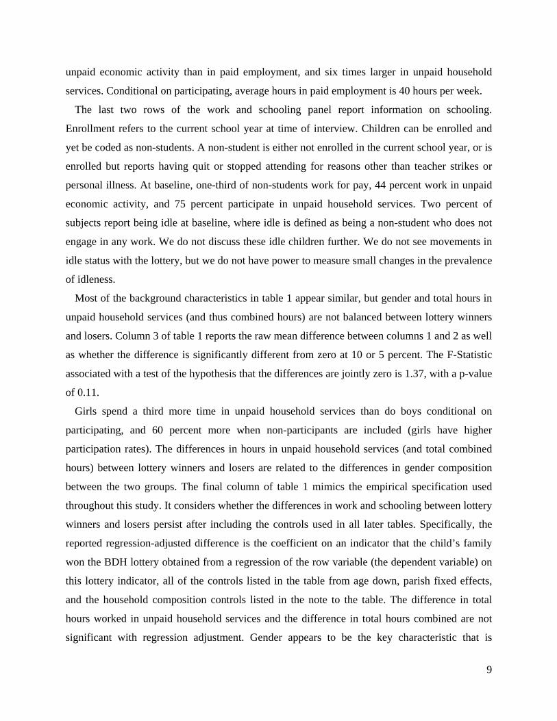
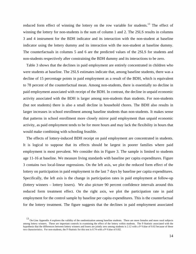
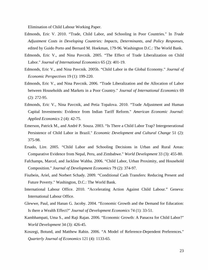
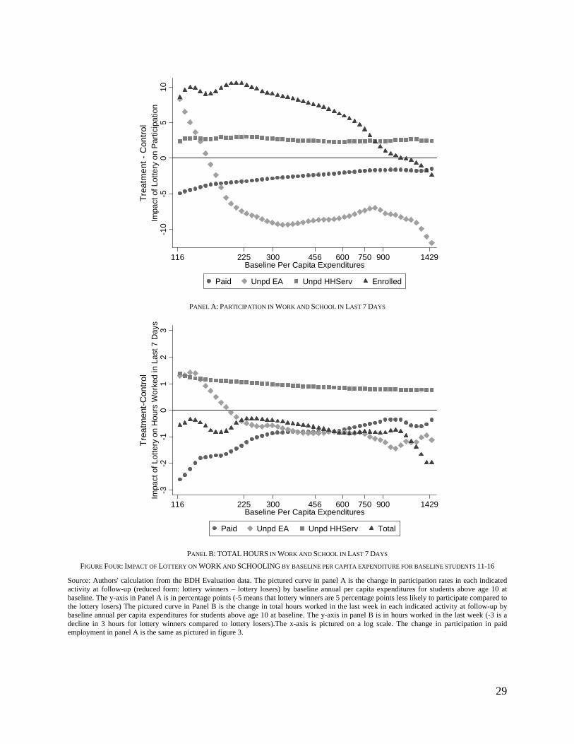
Figure 4 plots the impact of the lottery on participation in work and school as well as hours

worked. Each curve is generated in a manner identical the reduced form treatment effect with the

left axis in figure 3. Panel A reports changes in participation rates, and Panel B considers

changes in hours.16 Confidence bounds are not pictured to preserve readability. The figure shows

that the lottery leads to increases in school enrollment for all but the wealthiest 5 percent of

households at baseline. Unpaid household services increase throughout. Participation in unpaid

work in the family farm or business decreases among all but the poorest households. In the

poorest families, the lottery seems to induce a switch from paid employment to unpaid work in

the family farm or business, but total hours still decline. This substitution to unpaid work is

consistent with our hypothesis that the rigidity in paid employment hours is an important factor

in why paid employment is so responsive to the transfer.

C. Interpretation

The discussion in section I emphasized that additional income may affect child time allocation

through preferences for child schooling (or child welfare more generally), liquidity constraints,

need for child labor with self-insurance, changing the return to education, or altering the

productivity of child time in household-based production. We argue that preferences for child

welfare combined with rigidity in hours in paid employment are the simplest explanation for the

pattern of responses to the BDH we observe.

14

Half of the population in paid employment in the control sample at follow-up comes from families with baseline per capita expenditures below $380. Three-fourths come from families with baseline per capita expenditures below $490.

15 An obvious concern with comparisons of the type in Figure 3 is whether the randomization remains valid at such a fine partitioning of the

data. In the On-Line Appendix 5, we plot the probability a child's household wins the lottery by baseline per capita expenditures. The probability a household is a lottery winner appears balanced throughout the baseline per capita expenditure distribution.

16 We do not have data on changes in hours in school, so these are not included in the bottom panel. It is reasonable to assume that hours in

school are fixed, conditional on participation.

16

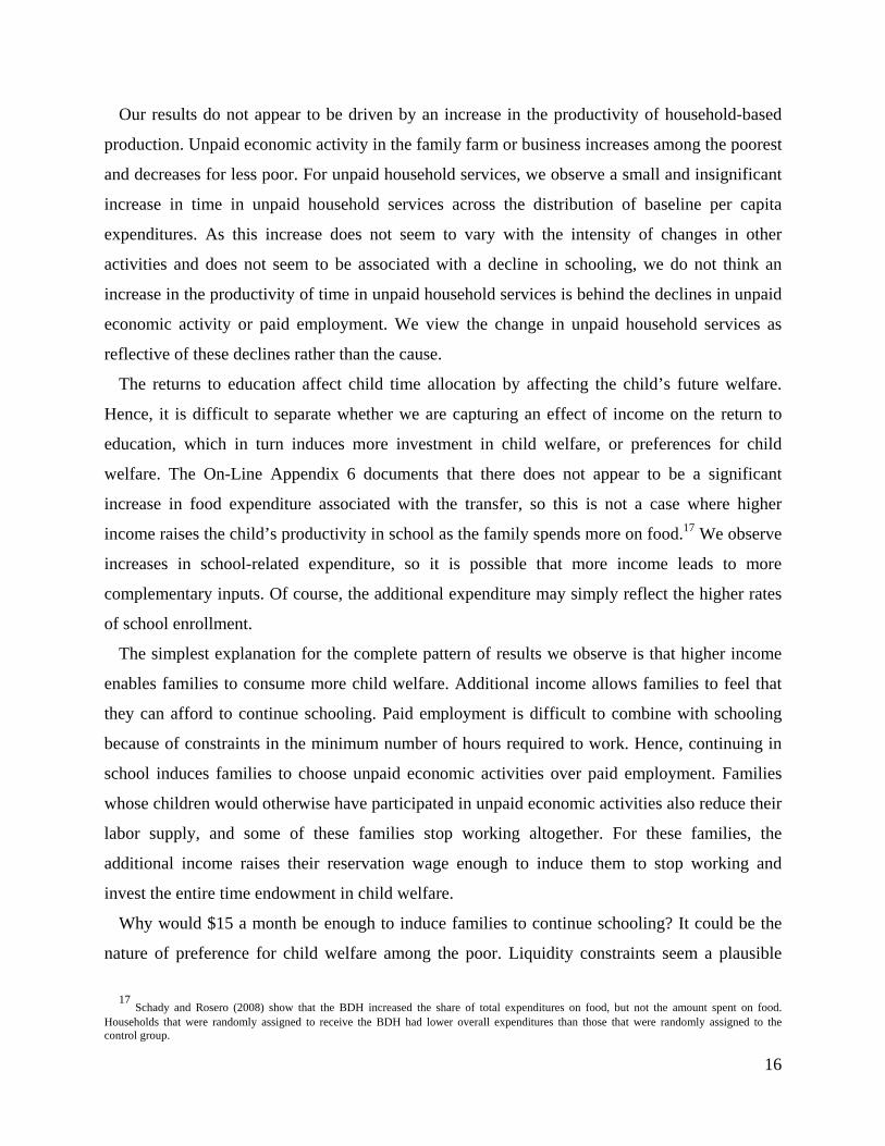
Our results do not appear to be driven by an increase in the productivity of household-based

production. Unpaid economic activity in the family farm or business increases among the poorest

and decreases for less poor. For unpaid household services, we observe a small and insignificant

increase in time in unpaid household services across the distribution of baseline per capita

expenditures. As this increase does not seem to vary with the intensity of changes in other

activities and does not seem to be associated with a decline in schooling, we do not think an

increase in the productivity of time in unpaid household services is behind the declines in unpaid

economic activity or paid employment. We view the change in unpaid household services as

reflective of these declines rather than the cause.

The returns to education affect child time allocation by affecting the child’s future welfare.

Hence, it is difficult to separate whether we are capturing an effect of income on the return to

education, which in turn induces more investment in child welfare, or preferences for child

welfare. The On-Line Appendix 6 documents that there does not appear to be a significant

increase in food expenditure associated with the transfer, so this is not a case where higher

income raises the child’s productivity in school as the family spends more on food.17 We observe

increases in school-related expenditure, so it is possible that more income leads to more

complementary inputs. Of course, the additional expenditure may simply reflect the higher rates

of school enrollment.

The simplest explanation for the complete pattern of results we observe is that higher income

enables families to consume more child welfare. Additional income allows families to feel that

they can afford to continue schooling. Paid employment is difficult to combine with schooling

because of constraints in the minimum number of hours required to work. Hence, continuing in

school induces families to choose unpaid economic activities over paid employment. Families

whose children would otherwise have participated in unpaid economic activities also reduce their

labor supply, and some of these families stop working altogether. For these families, the

additional income raises their reservation wage enough to induce them to stop working and

invest the entire time endowment in child welfare.

Why would $15 a month be enough to induce families to continue schooling? It could be the

nature of preference for child welfare among the poor. Liquidity constraints seem a plausible 17

Schady and Rosero (2008) show that the BDH increased the share of total expenditures on food, but not the amount spent on food. Households that were randomly assigned to receive the BDH had lower overall expenditures than those that were randomly assigned to the control group.

17

explanation, meaning families would have liked children to continue with school given current

prices (wages, returns to education) but were unable to do so. They may have difficulty dealing

with the lumpiness or the cash nature of school expenses, and they cannot borrow against future

earnings. The size of the transfer is slightly more than the average increase in schooling costs

between primary and secondary school, when many children end their schooling. However,

liquidity constraints are unlikely to be the entire story as the largest declines in unpaid economic

activity are among the least poor students, for whom there appears to be no substantive change in

school enrollment. $15 could also be enough to enable households to self-insure against the types

of shocks that occur with frequency. Hence, preference, liquidity constraints, and self-insurance

are all difficult to rule out as explanations for the observed declines in paid employment and

increases in schooling.

A potential concern with our results is that they reflect misunderstanding of the program. The

BDH experiment was conducted at a time when the government of Ecuador was emphasizing the

importance of the BDH for the accumulation of human capital. 25 percent of our sample (split

evenly between treatment and control) think that BDH recipients are supposed to attend school.

Schady and Araujo (2008) point out that, within the treated population, the increases in schooling

over time are largest for those who erroneously believe that they are supposed to attend school to

receive the BDH. Could mistaken beliefs about conditionality drive the changes in time

allocation we report?

Two pieces of evidence suggest that this is not the case. First, the social marketing campaign

emphasized the importance of schooling but did not address paid employment or any other

component of child labor. In fact, as we show, baseline students frequently combine school and

unpaid work in response to the transfer. Second, our results do not vary substantively with

beliefs about the schooling requirements of the transfer. Beliefs about schooling requirements are

not random, but we examine whether the impact of the lottery-induced take-up of the BDH on

child labor varies with these beliefs (measured only at follow-up) in table 4. The impact of the

lottery on paid employment and unpaid economic activity is not substantially larger among

children in households that report mistaken beliefs about conditionality. The only margin where

18

reported beliefs about schooling requirements substantively change the estimated effects of the

BDH is in school enrollment.18

IV. Conclusion

This study considers child time allocation responses to a lottery in Ecuador where women with

children were randomly assigned to receive $15 per month through the Bono de Desarrollo

Humano (BDH) program. Winning this lottery is associated with an increase in income.

Additional income allows families to feel that they can afford to continue schooling among those

in school at baseline. Paid employment is difficult to combine with schooling because of rigidity

in hours. Hence, continuing in school induces families to have children work in unpaid economic

activities rather than paid employment. Although those that stop paid employment are below

average earners, these families are typically giving up more in foregone child earnings than the

amount of the transfer.19 For families whose children would have engaged in unpaid economic

activity absent the transfer, the additional income induces substantial exit from the economically

active labor force.

The program effects we estimate are large in magnitude. Our 2SLS results suggest reductions

in paid employment of 10 percentage points (from a counterfactual mean of 24 percent), and

reductions in unpaid economic activity of 19 percentage points (from a counterfactual mean of

55 percent). Magnitudes are even larger for baseline students where we have a prior that the

transfer should be most effective. We compare the magnitude of these full sample effects with

those estimated for conditional cash transfer programs in Mexico, Nicaragua, and Colombia.

Skoufias and Parker (2001) estimate the effect of the PROGRESA program in Mexico on child

economic activity. They find that PROGRESA reduced economic activity among boys aged 12

to 17 by 3 to 5 percentage points, from a baseline value of 38 percent, and among girls by 2

percentage points, from a baseline value of 17 percent. Maluccio and Flores (2005) estimate that

the Red de Protección Social program in Nicaragua reduced economic activity by 3-5 percentage

points, although their analysis focuses on younger children, ages 7-12. Attanasio et al. (2010)

find no evidence that the Familias en Acción program in Colombia had an effect on child work

18

Of course, as Schady and Araujo (2008) emphasize, this is also the place where interpretation is most difficult since both treatment and control children who are attending school answer that they are supposed to attend school with the BDH. It is possible that children attending school simply respond that they are supposed to attend school, or that parents use misinformation about the transfer to coerce schooling out of children who otherwise might not attend.

19 Less than 2 percent of children in paid employment report earning less than $15 a month.

19

in income-generating activities (as opposed to unpaid household services) in either rural or urban

areas. The baseline values of the fraction working in income-generating activities in their sample

are 15 percent in rural areas, and 13 percent in urban areas. The large magnitude of the effects

we estimate is particularly surprising given the fact that the programs in Mexico, Nicaragua, and

Colombia made transfers that were conditional on school enrollment, while the BDH transfers

did not have strings attached to them.

There are a variety of reasons that could account for the large magnitude of the BDH effects

on child time allocation, relative to others in the literature. A much larger fraction of the children

in our sample work in paid employment than is the case in the studies described above, creating a

larger margin for declines in Ecuador than elsewhere. In addition, our estimated treatment effects

apply only to households for whom transfer take-up was affected by the BDH lottery. These

households are likely to be less “pushy” than others (meaning they did not get BDH benefits

except through the lottery), and the foregone earnings from switching children out of paid

employment appear to be below average. It might be particularly easy to affect the time

allocation of households such as these, and they may differ substantively from other households.

We think this group, whose behavior was affected by the BDH lottery, is one of policy interest.

At the moment, virtually every country in Latin America already has a cash transfer program, but

most cover only a fraction of poor households (see Fiszbein and Schady 2009, especially pp. 67-

80). In many contexts, then, households who are most “pushy” are likely to already have made

their way into existing programs. Therefore, if the policy that is being considered is the

expansion of the BDH or a similar program with less than full coverage of the poor, the

parameters we estimate in this paper may be a reasonable approximation to the expected effects

on child labor.

It is possible to interpret these findings as supporting some of the more controversial

assumptions within Basu and Van’s (1998) canonical model of child labor. Basu and Van rests

on an ad-hoc characterization of preferences known as the luxury axiom. The luxury axiom treats

preferences over child labor as lexicographic: child labor occurs if and only if families cannot

cover their subsistence needs without child labor. This ad-hoc characterization of preferences has

drawn substantial criticism. It implies that small changes in income can reduce child labor if it

moves families from below to above subsistence, and that the increase in income does not need

to cover foregone earnings. In the sample we study, we observe that a transfer valued at 7

20

percent of monthly expenditures is associated with a 41 percent reduction in paid employment.

We argue that the key factor behind these large reductions in paid employment is the presence of

rigidity in hours in paid employment. Basu and Van do not define child labor, but paid

employment was the standard empirical implementation of child labor in studies at the time. We

cannot say whether the transfer moves families from below subsistence to a point above, but

classical preferences and a binding constraint on the minimum number of hours in paid

employment appear to explain a set of results that are consistent with the luxury axiom

characterization of preferences in Basu and Van.

Our main findings on paid employment do not seem to be driven by mistaken perceptions of

BDH program requirements, but it is reasonable to suppose that the social context and the extent

to which parents perceive the transfer as permanent or temporary are important. The

government’s social marketing campaign could have shaped agent priorities for spending. It is

also plausible that government transfers are treated differently from found money or other

sources of income, so that agents may prioritize spending them on goods with greater social

returns, or there could be mental accounting issues involved. The fact that the transfer was new

may also be important in explaining its impact. Agents with children on the cusp of transitioning

between primary school to either secondary school or the labor market could respond to a

surprise $15 a month differently than they would have responded to an entirely anticipated

income source (regardless of whether they expect $15 a month to be transitory or permanent).

For example, suppose that a parent had calculated that their child would need to end schooling at

the end of primary because of the increase in school costs that accompany the transition to

secondary school. $15 a month is enough to cover the expected increase in schooling costs

between primary and secondary, and this "found money" might create the perception that the

family can now afford to delay entry to paid employment in a way that they would not have if

$15 had been included in the original budget for the household's optimization problem. The

experiment is not designed to test whether the income elasticity of paid employment is sensitive

to how the income is delivered.

Our findings highlight the central role that poverty plays in the child labor decision, and

suggest the possibility of affecting large changes in child labor with relatively modest

investments in poverty relief. Other studies have suggested the possibility of intergenerational

poverty traps working through child labor itself (Emerson and Souza 2003), its impact on

21

education (Barham et al. 1995), or the influence of child labor on occupational choice (Banerjee

and Newman 1993). It is difficult to predict the magnitude of the resulting multiplier effects from

child labor reductions, but taken together these studies and our results raise the prospect of large

returns to poverty alleviation programs.

REFERENCES

Attanasio, Orazio, Emla Fitzsimons, Ana Gomez, Martha I. Gutierrez, Costas Meghir, and Alice

Mesnard. 2010. “Children’s Schooling and Work in the Presence of a Conditional Cash

Transfer Program in Rural Colombia." Economic Development and Cultural Change 58 (2):

181-210.

Baland, Jean-Marie, and James A. Robinson. 2000. “Is Child Labor Inefficient?" Journal of

Political Economy 108 (4): 663-679.

Banerjee, Abhijit V., and Andrew F. Newman. 1993. “Occupational Choice and the Process of

Development.” Journal of Political Economy 101 (2): 274-298.

Barham, Vicky, Robin Boadway, Maurice Marchand, and Pierre Pestieau. 1995. “Education and

the Poverty Trap." European Economic Review 39 (7): 1257–75.

Basu, Kaushik, and Pham H. Van. 1998. “The Economics of Child Labor." American Economic

Review 88 (3): 412-427.

Basu, Kaushik, Sanghamitra Das, and Bhaskar Dutta. 2010. “Child Labor and Household

Wealth: Theory and Empirical Evidence of an Inverted-U." Journal of Development

Economics 91 (1): 8-14.

Beegle, Kathleen, Rajeev Dehejia, and Roberta Gatti. 2006. “Child Labor and Agricultural

Shocks." Journal of Development Economics 81(1): 80-96.

Behrman, Jere R., and James C. Knowles. 1999. “Household Income and Child Schooling in

Vietnam." World Bank Economic Review 13 (2): 211-56.

Bhalotra, Sonia, and Christopher Heady. 2003. “Child Farm Labor: The Wealth Paradox." World

Bank Economic Review 17 (2): 197-227.

Camacho, Adriana, and Emily Conover. 2011. “Manipulation of Social Program Eligibility."

American Economic Journal: Economic Policy 3 (2): 41-65.

Chetty, Raj, and Adam Szeidl. 2010. “Consumption Commitments: A Foundation for Reference-

Dependent Preferences and Habit Formation."

22

http://emlab.berkeley.edu/~szeidl/papers/commit_habit.pdf.

Chiwaula, Levison S. 2010. “Household Poverty and Child Labor Decisions in Malawi."

Research in Labor Economics 31: 33-51.

Cogneau, Denis, and Remi Jedwab. 2008. “Family Income and Child Outcomes: The 1990

Cocoa Price Shock in Cote d'Ivoire." Brunel University Centre for Economic Development

and Institutions Discussion Paper 08-13.

Dammert, Ana C. 2006. “Child Labor Response to Changes in Coca Production: Evidence from

Rural Peru." Unpublished.

Dammert, Ana C. 2008. “Child Labor and Schooling Response to Changes in Coca Production in

Rural Peru," Journal of Development Economics 86 (1): 164-80.

De Carvalho Filho, Irineu E. 2008. “Household Income as a Determinant of Child Labor and

School Enrollment in Brazil: Evidence from a Social Security Reform." International

Monetary Fund Working Paper 08/241.

De Janvry, Alain, Frederico Finan, Elizabeth Sadoulet, and Renos Vakis. 2005. “Can

Conditional Cash Transfers Serve as Safety Nets to keep Children at School and Out of the

Labor Market?” Journal of Development Economics 79(2): 349-373.

Dillon, Andrew. 2008. “Child Labor and Schooling Responses to Production and Health Shocks

in Northern Mali." International Food Policy Research Institute Discussion Paper 00755.

Doepke, Matthias, and Fabrizio Zilibotti. 2005. “The Macroeconomics of Child Labor

Regulation." American Economic Review 95 (5): 1492-1524.

Dumas, Christelle. 2007. “Why Do Parents Make Their Children Work? A Test of the Poverty

Hypothesis in Rural Areas of Burkina Faso." Oxford Economic Papers 59 (2): 301-29.

Duryea, Suzanne, David Lam, and Deborah Levison. 2007. “Effects of Economic Shocks on

Children's Employment and Schooling in Brazil.” Journal of Development Economics 84 (1):

188-214.

Edmonds, Eric V. 2005. “Does Child Labor Decline with Improving Economic Status?" Journal

of Human Resources 40 (1): 77-99.

Edmonds, Eric V. 2006. “Child Labor and Schooling responses to Anticipated Income in South

Africa." Journal of Development Economics 81(2): 386-414.

Edmonds, Eric V. 2008. “Defining Child Labour: A Review of the Definitions of Child Labour

in Policy Research." International Labour Organization International Programme on the

23

Elimination of Child Labour Working Paper.

Edmonds, Eric V. 2010. “Trade, Child Labor, and Schooling in Poor Countries." In Trade

Adjustment Costs in Developing Countries: Impacts, Determinants, and Policy Responses,

edited by Guido Porto and Bernard M. Hoekman, 179-96. Washington D.C.: The World Bank.

Edmonds, Eric V., and Nina Pavcnik. 2005. “The Effect of Trade Liberalization on Child

Labor." Journal of International Economics 65 (2): 401-19.

Edmonds, Eric V., and Nina Pavcnik. 2005b. “Child Labor in the Global Economy." Journal of

Economic Perspectives 19 (1): 199-220.

Edmonds, Eric V., and Nina Pavcnik. 2006. “Trade Liberalization and the Allocation of Labor

between Households and Markets in a Poor Country." Journal of International Economics 69

(2): 272-95.

Edmonds, Eric V., Nina Pavcnik, and Petia Topalova. 2010. “Trade Adjustment and Human

Capital Investments: Evidence from Indian Tariff Reform." American Economic Journal:

Applied Economics 2 (4): 42-75.

Emerson, Patrick M., and André P. Souza. 2003. “Is There a Child Labor Trap? Intergenerational

Persistence of Child Labor in Brazil." Economic Development and Cultural Change 51 (2):

375-98.

Ersado, Lire. 2005. “Child Labor and Schooling Decisions in Urban and Rural Areas:

Comparative Evidence from Nepal, Peru, and Zimbabwe." World Development 33 (3): 455-80.

Fafchamps, Marcel, and Jackline Wahba. 2006. “Child Labor, Urban Proximity, and Household

Composition." Journal of Development Economics 79 (2): 374-97.

Fiszbein, Ariel, and Norbert Schady. 2009. “Conditional Cash Transfers: Reducing Present and

Future Poverty." Washington, D.C.: The World Bank.

International Labour Office. 2010. “Accelerating Action Against Child Labour.” Geneva:

International Labour Office.

Glewwe, Paul, and Hanan G. Jacoby. 2004. “Economic Growth and the Demand for Education:

Is there a Wealth Effect?" Journal of Development Economics 74 (1): 33-51.

Kambhampati, Uma S., and Raji Rajan. 2006. “Economic Growth: A Panacea for Child Labor?"

World Development 34 (3): 426-45.

Koszegi, Botund, and Matthew Rabin. 2006. “A Model of Reference-Dependent Preferences."

Quarterly Journal of Economics 121 (4): 1133-65.

24

Kruger, Diana I. 2007. “Coffee Production Effects on Child Labor and Schooling in Rural

Brazil." Journal of Development Economics 82 (2): 448-63.

Jacoby, Hanan G., and Emmanuel Skoufias. 1997. “Risk, Financial Markets, and Human Capital

in a Developing Country." Review of Economic Studies 64 (3): 311-35.

Maluccio, John A., and Rafael Flores. 2005. “Impact Evaluation of a Conditional Cash Transfer

Program: the Nicaraguan Red de Protección Social." Research Report 141. Washington, D.C.:

International Food Policy Research Institute.

Manacorda, Marco. 2006. “Child Labor and the Labor Supply of Other Household Members:

Evidence from 1920 America. " American Economic Review 96 (5): 1788-1801.

Manacorda, Marco, and Furio C. Rosati. 2010. “Local Labor Demand and Child Work."

Research in Labor Economics 31: 321-54.

Mueller, Eva. 1984. “The Value and Allocation of Time in Rural Botswana." Journal of

Development Economics 15 (1-3): 329-60.

Paxson, Christina, and Norbert Schady. 2010. “Does Money Matter? The Effects of Cash

Transfers on Child Development in Rural Ecuador." Economic Development and Cultural

Change 59 (1): 187-230.

Psacharopoulos, George. 1997. “Child Labor versus Educational Attainment: Some Evidence

from Latin America." Journal of Population Economics 10 (4): 377-86.

Ranjan, Priya. 2001. “Credit Constraints and the Phenomenon of Child Labor." Journal of

Development Economics 64 (1): 81-102.

Ray, Ranjan. 2000. “Analysis of Child Labour in Peru and Pakistan: A Comparative Study."

Journal of Population Economics 13 (1): 3-19.

Rosenzweig, Mark R., and Robert Evenson, 1977. “Fertility, Schooling, and the Economic

Contribution of Children in Rural India: An Econometric Analysis." Econometrica 45 (5):

1065-79.

Schady, Norbert. 2004. “Do Macroeconomic Crises Always Slow Human Capital

Accumulation?" World Bank Economic Review 18 (2): 131-54.

Schady, Norbert, and Maria C. Araujo. 2008. “Cash Transfers, Conditions, and School

Enrollment in Ecuador" Economía 8 (2): 43-70.

Schady, Norbert, and José Rosero. 2008. “Are Cash Transfers Made to Women Spent Like Other

Sources of Income?" Economics Letters 101 (3): 246-48.

25

Schultz, T. Paul. 2004. “School Subsidies for the Poor: Evaluating the Mexican Progresa Poverty

Program." Journal of Development Economics 74 (1): 199-250.

Schultz, Theodore W. 1960. “Capital Formation by Education.” Journal of Political Economy 68

(6): 571-83.

Skoufias, Emmanuel, and Susan W. Parker. 2001. “Conditional Cash Transfers and Their Impact

on Child Work and Schooling: Evidence from the PROGRESA Program in Mexico."

Economía 2 (1): 45-86.

Swaminathan, Madhura. 1998. “Economic Growth and the Persistence of Child Labor: Evidence

from an Indian City." World Development 26 (8): 1513-28.

Wahba, Jackline. 2006. “The Influence of Market Wages and Parental History on Child Labour

and Schooling in Egypt." Journal of Population Economics 19 (4): 823-52.

Yang, Dean. 2008. "International Migration, Remittances, and Household Investment: Evidence

from Philippine Migrants' Exchange Rate Shocks." Economic Journal 118 (528): 591-630.

26

FIGURE ONE: PARTICIPATION IN WORK AND SCHOOL AT BASELINE BY AGE

Source: Authors' calculation from the BDH Evaluation data at baseline.

020

4060

8010

0

5 6 7 8 9 10 11 12 13 14 15 16Age at Baseline

Paid Emp Unpaid Economic ActivityDomestic Work In School

Par

tici

pati

on R

ate

27

FIGURE TWO: THE DISTRIBUTION OF HOURS WORKED IN PAID EMPLOYMENT IN THE CONTROL POPULATION AT FOLLOW-UP Source: BDH Evaluation control sample at follow-up data. We focus on the control population at follow-up for this figure rather than the baseline population, because the baseline population is on average 1.5 years younger than is the population at follow-up. Age 11-16 at baseline. The bin width is 5 hours.

0.0

2.0

4.0

6.0

8D

ensi

ty

0 5 10 15 20 25 30 35 40 45 50 55 60 65 70 75 80 85 90Total Hours Worked For Pay in Lasy 7 Days

28

FIGURE THREE: IMPACT OF THE LOTTERY BY BASELINE PER CAPITA EXPENDITURE FOR BASELINE STUDENTS AGE 11-16 Authors' calculation from the BDH Evaluation data. The pictured solid curve is the change in participation rates in wage employment at follow-up (reduced form: lottery winners – lottery losers) by baseline annual per capita expenditures for students above age 10 at baseline. The pictured dotted curve is the mean incidence of wage employment among lottery losers at follow-up by baseline annual per capita expenditures for students above age 10 at baseline. The x-axis is pictured on a log scale. The y-axis is in percentage points (5 is 5 percentage points). 90 percent confidence interval for the change in participation rates is pictured.

Treatment Effect (left axis)

Counterfactual (right axis)

1010

.511

11.5

1212

.5P

aid

Em

ploy

men

t

-8-6

-4-2

02

116 225 300 456 600 750 900 1429Per Capita Expenditures at Baseline

Con

trol

Gro

up P

arti

cipa

tion

Rat

e

Cha

nge

in P

aid

Em

ploy

men

t, T

reat

men

t - C

ontr

ol

29

PANEL A: PARTICIPATION IN WORK AND SCHOOL IN LAST 7 DAYS

PANEL B: TOTAL HOURS IN WORK AND SCHOOL IN LAST 7 DAYS

FIGURE FOUR: IMPACT OF LOTTERY ON WORK AND SCHOOLING BY BASELINE PER CAPITA EXPENDITURE FOR BASELINE STUDENTS 11-16 Source: Authors' calculation from the BDH Evaluation data. The pictured curve in panel A is the change in participation rates in each indicated activity at follow-up (reduced form: lottery winners – lottery losers) by baseline annual per capita expenditures for students above age 10 at baseline. The y-axis in Panel A is in percentage points (-5 means that lottery winners are 5 percentage points less likely to participate compared to the lottery losers) The pictured curve in Panel B is the change in total hours worked in the last week in each indicated activity at follow-up by baseline annual per capita expenditures for students above age 10 at baseline. The y-axis in panel B is in hours worked in the last week (-3 is a decline in 3 hours for lottery winners compared to lottery losers).The x-axis is pictured on a log scale. The change in participation in paid employment in panel A is the same as pictured in figure 3.

-10

-50

51

0Im

pact

of L

otte

ry o

n P

artic

ipa

tion

116 225 300 456 600 750 900 1429Baseline Per Capita Expenditures

Paid Unpd EA Unpd HHServ Enrolled

Tre

atm

ent

- C

ontr

ol

-3-2

-10

12

3Im

pact

of L

otte

ry o

n H

our

s W

ork

ed in

La

st 7

Da

ys

116 225 300 456 600 750 900 1429Baseline Per Capita Expenditures

Paid Unpd EA Unpd HHServ Total

Tre

atm

ent

-Con

tro

l

Variable (b/se)Lottery Winners

Lottery Losers

Mean Difference

Regression Adjusted

DifferenceSample Size 993 890 1,883 1,883

Paid Employment 0.14 0.14 0.00 0.00(0.01) (0.01) (0.02) (0.02)

Unpaid Economic Activity 0.42 0.42 0.00 0.01(0.02) (0.02) (0.03) (0.02)

Any Economic Activity 0.53 0.53 0.00 0.00(0.02) (0.02) (0.03) (0.02)

Unpaid Household Services 0.83 0.83 0.00 -0.01(0.01) (0.01) (0.02) (0.02)

Any Work 0.93 0.93 0.00 0.00(0.01) (0.01) (0.01) (0.01)

Total Hours Last Week, Paid Employment 4.09 4.02 0.08 0.13(0.39) (0.40) (0.48) (0.51)

Total Hours, Unpaid Economic Activity 6.12 5.51 0.60 0.40(0.35) (0.33) (0.52) (0.44)

Total Hours Last Week, Economic Activity 10.22 9.53 0.68 0.52(0.50) (0.50) (0.64) (0.64)

Total Hours Last Week, Unpaid Hh. Services 9.45 8.68 0.76** 0.29(0.29) (0.28) (0.37) (0.41)

Total Hours Last Week, Combined 19.67 18.21 1.44** (0.80)(0.56) (0.57) (0.70) (0.77)

Total Earnings Last Month Paid Employment 9.85 9.76 0.18 0.44(1.05) (1.13) (2.04) (2.01)

School Enrollment 0.66 0.66 0.00 0.01(0.02) (0.02) (0.03) (0.03)

Non-student 0.35 0.34 0.00 -0.01(0.02) (0.02) (0.03) (0.03)

Age (at baseline) 13.43 13.45 -0.02 n/a(0.05) (0.05) (0.06)

Male 0.47 0.52 -0.05** n/a(0.02) (0.02) (0.02)

Speaks Indigenous Language 0.10 0.08 0.02 n/a(0.01) (0.01) (0.02)

Has Disability 0.01 0.01 0.00 n/a(0.00) (0.00) (0.01)

Oldest Resident Child 0.65 0.66 -0.01 n/a(0.02) (0.02) (0.02)

Oldest Resident Girl 0.42 0.39 0.02 n/a(0.02) (0.02) (0.02)

Mother Present 0.94 0.93 0.00 n/a(0.01) (0.01) (0.02)

Mother's Years of Education 3.70 3.46 0.25 n/a(0.09) (0.10) (0.16)

Father Present 0.82 0.83 -0.01 n/a(0.01) (0.01) (0.03)

Rural Locality 0.53 0.50 0.04 n/a(0.02) (0.02) (0.04)

# School Age Children Present 2.70 2.60 0.10 n/a(0.04) (0.04) (0.09)

# Children 0 to 5 Present 0.51 0.46 0.05 n/a(0.02) (0.02) (0.05)

Log of Per Capita Expenditures 6.00 6.01 -0.01 n/a(0.02) (0.02) (0.03)

Household Size 6.14 6.09 0.04 n/a(0.06) (0.06) (0.12)

All characteristics are at baseline. Regression adjustment includes parish fixed effects and all controls from "Age" down to "Total Monthly Expenditure" marked with "n/a" plus counts of the number of men and women (separately) present at baseline and follow-up in each of the following age categories: under 5, 6-17, 18-44, 45-64, 65+. Household Size, Age, # school age, and # children are included as dummy variables in all regressions. For each characteristics, the standard error is reported on the line below the mean. Standard errors are corrected for clustering at the parish level. ** is significant at 5 percent. * is significant at 10 percent.

Table 1: Differences in Subject Characteristics at Baseline by Treatment Status

Ind

ivid

ual

Ch

arac

teri

stic

sW

ork

an

d S

choo

ling

Hou

seh

old

Ch

arac

teri

stic

s

Children 11-16 at baseline

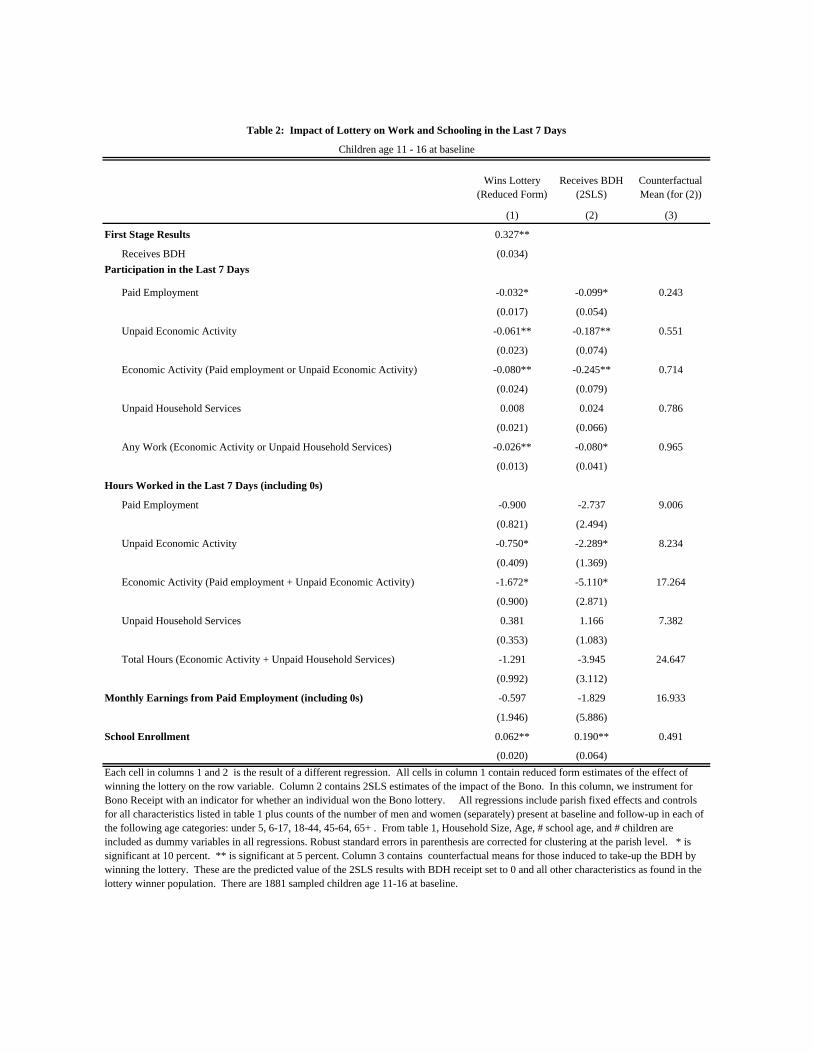
Wins Lottery (Reduced Form)

Receives BDH (2SLS)

Counterfactual Mean (for (2))

(1) (2) (3)

First Stage Results 0.327**

Receives BDH (0.034)

Paid Employment -0.032* -0.099* 0.243

(0.017) (0.054)

Unpaid Economic Activity -0.061** -0.187** 0.551

(0.023) (0.074)

Economic Activity (Paid employment or Unpaid Economic Activity) -0.080** -0.245** 0.714

(0.024) (0.079)

Unpaid Household Services 0.008 0.024 0.786

(0.021) (0.066)

Any Work (Economic Activity or Unpaid Household Services) -0.026** -0.080* 0.965

(0.013) (0.041)

Paid Employment -0.900 -2.737 9.006

(0.821) (2.494)

Unpaid Economic Activity -0.750* -2.289* 8.234

(0.409) (1.369)

Economic Activity (Paid employment + Unpaid Economic Activity) -1.672* -5.110* 17.264

(0.900) (2.871)

Unpaid Household Services 0.381 1.166 7.382

(0.353) (1.083)

Total Hours (Economic Activity + Unpaid Household Services) -1.291 -3.945 24.647

(0.992) (3.112)

-0.597 -1.829 16.933

(1.946) (5.886)

0.062** 0.190** 0.491

(0.020) (0.064)

School Enrollment

Each cell in columns 1 and 2 is the result of a different regression. All cells in column 1 contain reduced form estimates of the effect of winning the lottery on the row variable. Column 2 contains 2SLS estimates of the impact of the Bono. In this column, we instrument for Bono Receipt with an indicator for whether an individual won the Bono lottery. All regressions include parish fixed effects and controls for all characteristics listed in table 1 plus counts of the number of men and women (separately) present at baseline and follow-up in each of the following age categories: under 5, 6-17, 18-44, 45-64, 65+ . From table 1, Household Size, Age, # school age, and # children are included as dummy variables in all regressions. Robust standard errors in parenthesis are corrected for clustering at the parish level. * is significant at 10 percent. ** is significant at 5 percent. Column 3 contains counterfactual means for those induced to take-up the BDH by winning the lottery. These are the predicted value of the 2SLS results with BDH receipt set to 0 and all other characteristics as found in the lottery winner population. There are 1881 sampled children age 11-16 at baseline.

Table 2: Impact of Lottery on Work and Schooling in the Last 7 Days

Children age 11 - 16 at baseline

Participation in the Last 7 Days

Hours Worked in the Last 7 Days (including 0s)

Monthly Earnings from Paid Employment (including 0s)

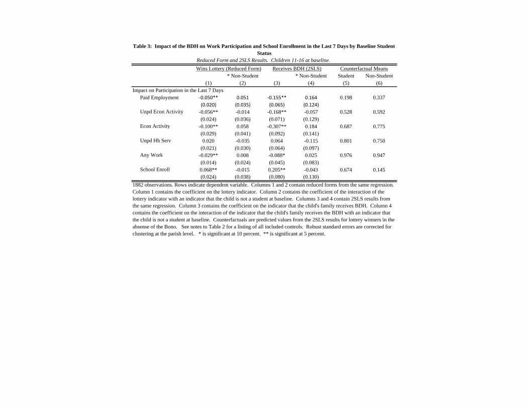
* Non-Student * Non-Student Student Non-Student(1) (2) (3) (4) (5) (6)

Impact on Participation in the Last 7 DaysPaid Employment ‐0.050** 0.051 ‐0.155** 0.164 0.198 0.337

(0.020) (0.035) (0.065) (0.124)Unpd Econ Activity -0.056** -0.014 -0.168** -0.057 0.528 0.592

(0.024) (0.036) (0.071) (0.129)Econ Activity -0.100** 0.058 -0.307** 0.184 0.687 0.775

(0.029) (0.041) (0.092) (0.141)Unpd Hh Serv 0.020 -0.035 0.064 -0.115 0.801 0.750

(0.021) (0.030) (0.064) (0.097)Any Work -0.029** 0.008 -0.088* 0.025 0.976 0.947

(0.014) (0.024) (0.045) (0.083)School Enroll 0.068** -0.015 0.205** -0.043 0.674 0.145

(0.024) (0.038) (0.080) (0.130)

1882 observations. Rows indicate dependent variable. Columns 1 and 2 contain reduced forms from the same regression. Column 1 contains the coefficient on the lottery indicator. Column 2 contains the coefficient of the interaction of the lottery indicator with an indicator that the child is not a student at baseline. Columns 3 and 4 contain 2SLS results from the same regression. Column 3 contains the coefficient on the indicator that the child's family receives BDH. Column 4 contains the coefficient on the interaction of the indicator that the child's family receives the BDH with an indicator that the child is not a student at baseline. Counterfactuals are predicted values from the 2SLS results for lottery winners in the absense of the Bono. See notes to Table 2 for a listing of all included controls. Robust standard errors are corrected for clustering at the parish level. * is significant at 10 percent. ** is significant at 5 percent.

Table 3: Impact of the BDH on Work Participation and School Enrollment in the Last 7 Days by Baseline Student Status

Counterfactual MeansReceives BDH (2SLS)Wins Lottery (Reduced Form)

Reduced Form and 2SLS Results. Children 11-16 at baseline.

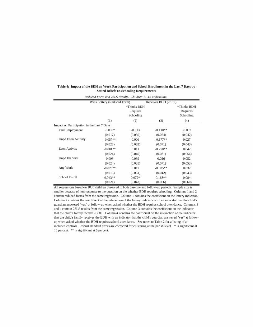
Wins Lottery (Reduced Form) Receives BDH (2SLS)

*Thinks BDH Requires Schooling

*Thinks BDH Requires Schooling

(1) (2) (3) (4)

Impact on Participation in the Last 7 Days

Paid Employment -0.033* -0.013 -0.110** -0.007

(0.017) (0.030) (0.054) (0.042)Unpd Econ Activity -0.057** 0.006 -0.177** 0.027

(0.022) (0.032) (0.071) (0.043)Econ Activity -0.081** 0.011 -0.250** 0.042

(0.024) (0.040) (0.081) (0.054)Unpd Hh Serv 0.003 0.039 0.026 0.052

(0.024) (0.035) (0.071) (0.053)Any Work -0.029** 0.017 -0.085** 0.032

(0.013) (0.031) (0.042) (0.043)School Enroll 0.043** 0.072* 0.168** 0.084

(0.021) (0.042) (0.066) (0.060)

All regressions based on 1835 children observed in both baseline and follow-up periods. Sample size is smaller because of non-response to the question on the whether BDH requires schooling. Columns 1 and 2 contain reduced forms from the same regression. Column 1 contains the coefficient on the lottery indicator. Column 2 contains the coefficient of the interaction of the lottery indicator with an indicator that the child's guardian answered "yes" at follow-up when asked whether the BDH requires school attendance. Columns 3 and 4 contain 2SLS results from the same regression. Column 3 contains the coefficient on the indicator that the child's family receives BDH. Column 4 contains the coefficient on the interaction of the indicator that the child's family receives the BDH with an indicator that the child's guardian answered "yes" at follow-up when asked whether the BDH requires school attendance. See notes to Table 2 for a listing of all included controls. Robust standard errors are corrected for clustering at the parish level. * is significant at 10 percent. ** is significant at 5 percent.

Table 4: Impact of the BDH on Work Participation and School Enrollment in the Last 7 Days by Stated Beliefs on Schooling Requirements

Reduced Form and 2SLS Results. Children 11-16 at baseline.