POUNDING AND IMPACT OF BASE ISOLATED BUILDINGS DUE …
149
POUNDING AND IMPACT OF BASE ISOLATED BUILDINGS DUE TO EARTHQUAKES A Thesis by VIVEK KUMAR AGARWAL Submitted to the Office of Graduate Studies of Texas A&M University in partial fulfillment of the requirements for the degree of MASTER OF SCIENCE May 2004 Major Subject: Civil Engineering
Transcript of POUNDING AND IMPACT OF BASE ISOLATED BUILDINGS DUE …

POUNDING AND IMPACT OF BASE ISOLATED BUILDINGS DUE TO
EARTHQUAKES
A Thesis
by
VIVEK KUMAR AGARWAL
Submitted to the Office of Graduate Studies of Texas A&M University
in partial fulfillment of the requirements for the degree of
MASTER OF SCIENCE
May 2004
Major Subject: Civil Engineering

POUNDING AND IMPACT OF BASE ISOLATED BUILDINGS DUE TO
EARTHQUAKES
A Thesis
by
VIVEK KUMAR AGARWAL
Submitted to Texas A&M University
in partial fulfillment of the requirements for the degree of
MASTER OF SCIENCE
Approved as to style and content by:
John M. Niedzwecki(Chair of Committee)
(Int
May 2004
Major Subject: Civil Engineer
Ken Reinschmidt(Member)
er )
H. Joseph Newton(Member)
in
Paul Roschke im Department Head
g

iii
ABSTRACT
Pounding and Impact of Base Isolated Buildings due to Earthquakes. (May 2004)
Vivek Kumar Agarwal, B. Tech.,
Indian Institute of Technology, Delhi, India
Chair of Advisory Committee: Dr. John M. Niedzwecki
As the cost of land in cities increases, the need to build multistory buildings in
close proximity to each other also increases. Sometimes, construction materials, other
objects and any projections from a building may also decrease the spacing provided
between the buildings. This leads to the problem of pounding of these closely placed
buildings when responding to earthquake ground motion. The recent advent of base
isolation systems and their use as an efficient earthquake force resisting mechanism has
led to their increased use in civil engineering structures. At the same time, building
codes that reflect best design practice are also evolving.
The movement of these base isolated buildings can also result in building pounding.
Since base isolation is itself a relatively new technique, pounding phenomenon in base
isolated buildings have not been adequately investigated to date. This study looks at the
base isolated response of a single two story building and adjacent two story building
systems. Four earthquakes with increasing intensity were used in this study. It was
found that it is difficult to anticipate the response of the adjacent buildings due to non-
linear behavior of pounding and base isolation. The worst case for pounding was found
to occur when a fixed base and base isolated buildings were adjacent to each other.

iv
DEDICATION
Dedicated to my mother Prem Lata Gupta and father Suresh Chandra Gupta who have
worked hard throughout for my education and gave me the opportunity to come to
United States for higher studies.

v
ACKNOWLEDGMENTS
I would like to take this opportunity to express my deep gratitude to my advisory
committee chair Dr. John M. Niedzwecki for giving me the opportunity to work on this
research project and his guidance throughout, to its completion. I would also like to
thank Dr. Ken Reinschmidt and Dr. H. Joseph Newton for being my committee members
and for their helpful suggestions.
Funding for this research project was provided by the US Department of Interior
Geological Survey under contract number 02HQGR0110 and the R. P. Gregory’32 Chair
Endowment. Their support to this project is gratefully acknowledged.

vi
TABLE OF CONTENTS
Page
ABSTRACT ..................................................................................................................... iii DEDICATION ..................................................................................................................iv ACKNOWLEDGMENTS..................................................................................................v TABLE OF CONTENTS ..................................................................................................vi LIST OF TABLES ......................................................................................................... viii LIST OF FIGURES...........................................................................................................ix 1. INTRODUCTION......................................................................................................1
1.1. Previous work on the subject .........................................................................2 1.2. Current state of practice ...............................................................................12
1.2.1. Fixed base buildings .....................................................................12 1.2.2. Base isolated buildings .................................................................12
1.3. Study objective.............................................................................................13 2. MATHEMATICAL FORMULATION ...................................................................15
2.1. Basic building pounding model ...................................................................15 2.1.1. Single degree of freedom systems ................................................15 2.1.2. Two degree of freedom systems...................................................20
2.2. Base isolated building system......................................................................24 2.2.1. Single degree of freedom system..................................................24 2.2.2. Two degree of freedom system ....................................................28
2.3. Base isolation with building pounding ........................................................32 2.3.1. Single degree of freedom systems ................................................32 2.3.2. Two degree of freedom systems...................................................36
3. VALIDATION OF THE NUMERICAL MODEL: FIXED BASE .........................41
3.1. Semi-analytic solution: 2-DOF building......................................................41 3.2. Pounding in fixed base buildings: 2-DOF model ........................................48

vii
Page 4. SIMULATION OF BUIILDING POUNDING WITH BASE ISOLATION ..........59
4.1. Single base isolated building .......................................................................59 4.2. Fixed base and base isolated adjacent buildings..........................................65 4.3. Base isolation in both adjacent buildings.....................................................72
5. SUMMARY AND CONCLUSION.........................................................................85
5.1. Summary and scope of study .......................................................................85 5.2. Conclusions..................................................................................................86 5.3. Recommendations for further study.............................................................88
REFERENCES.................................................................................................................90 APPENDIX 1 ...................................................................................................................94 APPENDIX 2 .................................................................................................................102 APPENDIX 3 .................................................................................................................110 APPENDIX 4 .................................................................................................................122 APPENDIX 5 .................................................................................................................134 VITA ..............................................................................................................................138

viii
LIST OF TABLES
TABLE Page
1.1 Survey of earlier research on pounding of buildings...............................................5
3.1 Adjacent building configurations used in this study..............................................49
3.2 Characterization of environment – Statistics for earthquakes ...............................51
3.3 Properties of Building 2.........................................................................................53
4.1 Response behavior characterization for varying friction coefficients. Building 1: base isolated, Building 2: stiff ...........................................................70
4.2 Response behavior characterization for earthquakes of increasing intensity.
Building 1: base isolated, Building 2: stiff ...........................................................70
4.3 Response behavior characterization for varying friction coefficients. Building 1: base isolated, Building 2: flexible ......................................................71
4.4 Response behavior characterization for earthquakes of increasing intensity.
Building 1: base isolated, Building 2: flexible ......................................................71
4.5 Response behavior characterization for varying friction coefficients. Both buildings: base isolated, Building 2: stiff ..............................................................77
4.6 Response behavior characterization for earthquakes of increasing intensity.
Both buildings: base isolated, Building 2: stiff .....................................................77
4.7 Response behavior characterization for varying friction coefficients. Both buildings: base isolated, Building 2: flexible ........................................................78
4.8 Response behavior characterization for earthquakes of increasing intensity.
Both buildings: base isolated, Building 2: flexible ...............................................78
4.9 Correlation coefficients, Building 2: stiff ..............................................................84
4.10 Correlation coefficients, Building 2: flexible ........................................................84

ix
LIST OF FIGURES
FIGURE Page
2.1 Schematic diagram of the three adjacent fixed base buildings..............................16
2.2 Free body diagram for lumped mass m11 of first floor of Building 1....................16
2.3 Free body diagram for lumped mass m21 of first floor of Building 2....................16
2.4 Free body diagram for lumped mass m31 of first floor of Building 3....................16
2.5 Schematic diagram of the two adjacent 2-DOF fixed base systems......................21
2.6 Schematic diagram of the single 1-DOF base isolated system..............................26
2.7 Free body diagram for lumped mass m11 of the first floor of 1-DOF base isolated system.......................................................................................................26
2.8 Free body diagram for lumped mass MB11 of the base of 1-DOF base
isolated system.......................................................................................................26
2.9 Schematic diagram of the single 2-DOF base isolated system..............................29
2.10 Free body diagram for lumped mass m12 of second floor .....................................29
2.11 Free body diagram for lumped mass m11 of first floor ..........................................29
2.12 Free body diagram for lumped mass MB11 of base ................................................29
2.13 Schematic diagram of the three adjacent 1-DOF base isolated systems................33
2.14 Schematic diagram of the two adjacent 2-DOF base isolated systems..................37
3.1 Reference building used for analysis .....................................................................43
3.2 Semi-analytical solution for 2-DOF system. Second floor response; First floor response ........................................................................................................46
3.3 Numerical solution for 2-DOF system. Second floor response; First floor
response .................................................................................................................47

x
FIGURE Page
3.4 Acceleration time histories for the earthquakes.....................................................50
3.5 Adjacent fixed base buildings................................................................................53
3.6 Response time history of Building 1; Impact forces; Building 2: Flexible, Gap = 2 cm ............................................................................................................55
3.7 Variation in number of impacts with increasing gap between the buildings.........56
3.8 Variation of peak displacement with increasing gap between the buildings.........57
3.9 Variation in peak impact force with increasing gap between the buildings ..........57
4.1 Skewness of total displacement response for different earthquakes......................60
4.2 Coefficient of excess of total displacement response for different earthquakes....60
4.3 Maximum relative displacement response for different earthquakes ....................62
4.4 Maximum sliding displacement response for different earthquakes .....................62
4.5 Maximum total displacement response for different earthquakes .........................63
4.6 Histograms and normal probability curve for the displacement response of
base isolated reference building subjected to different earthquakes .....................64
4.7 Adjacent base isolated and fixed base buildings ...................................................66
4.8 Total number of impacts as a function of Building 2 stiffness and base isolation friction coefficient in Building 1 ............................................................67
4.9 Maximum impact force as a function of Building 2 stiffness and base
isolation friction coefficient in Building 1 ............................................................67
4.10 Maximum duration of impacts as a function of Building 2 stiffness and base isolation friction coefficient in Building 1 ............................................................69
4.11 Total displacement as a function of Building 2 stiffness and base isolation
friction coefficient in Building 1 ...........................................................................69
4.12 Total number of impacts as a function of Building 2 stiffness and base isolation friction coefficient...................................................................................73

xi
FIGURE Page
4.13 Maximum impact force as a function of Building 2 stiffness and base isolation friction coefficient...................................................................................73
4.14 Maximum duration of impacts as a function of Building 2 stiffness and base
isolation friction coefficient...................................................................................74
4.15 Maximum total displacement as a function of Building 2 stiffness and base isolation friction coefficient...................................................................................74
4.16 Maximum relative displacement as a function of base isolation friction
coefficient with stiff Building 2.............................................................................75
4.17 Maximum relative displacement as a function of base isolation friction coefficient with flexible Building 2.......................................................................75
4.18 Histogram and normal probability density function of total displacement for
El Centro earthquake, Gap = 2 cm ........................................................................80
4.19 Histogram and normal probability density function of total displacement for Loma Prieta earthquake, Gap = 4 cm ....................................................................81
4.20 Time histories of total displacement for El Centro earthquake, µ = 0.2,
Gap = 2 cm ............................................................................................................82

1
1. INTRODUCTION
Building structures are often built close to each other as in the case of residential
building complexes or in downtown of metropolitan cities where the cost of land is high.
Due to the close proximity of these structures, they have often been found to impact each
other while responding to earthquake induced strong ground motion. An earthquake can
cause sudden movement of the ground that is transferred to the structure through
foundation. The ground motion during an earthquake is usually defined by a time
history of the ground acceleration and can be obtained in three directions by instruments
known as strong-motion accelerographs (see for example, Chopra 2001). Evaluating the
response of a building structure subjected to earthquake ground motion is a dynamic
problem where at any instant, the internal resisting forces of the structure are in
equilibrium with the time varying inertia force that is defined as the product of the
structural mass and the instantaneous ground acceleration (Clough and Penzien 1993).
To reduce the response of a structure to earthquake excitation, various types of base
isolation systems have been proposed. One approach is to modify foundation for a
building by introducing a layer of material that has a very low lateral stiffness, thus
reducing the natural period of vibration of structure. Another technique that is effective
in retrofitting structures is the use of a discrete number of friction bearings located
between the foundation and the superstructure. Once installed this allows the structure
to slide on its foundation during ground movement. The use of friction bearings reduces
the base shear force transferred to the structure and hence reduces the displacement of
the floors with respect to the base and the internal forces produced in the structure. They
can be designed to permit sliding of the structure only during very strong earthquakes. It
is this friction bearing base isolation technique that we will be incorporating in the
dynamic model formulated in this research study. 1
This thesis follows the style and format of the ASCE Journal of Structural Engineering.
2
The differences in geometrical and material properties of adjacent buildings can lead to
significant differences in their response to the external forces. Spatial variation of the
ground movement in case of an earthquake can also cause the adjacent structures to
respond differently. Consequently, adjacent buildings may vibrate quite differently
during earthquake and may impact each other at various times during their movement.
Due to the huge mass of buildings, the momentum of the vibrating structures is also
huge and can cause lot of local damage during an impact. In addition to this, large
impact forces can significantly change the response behavior during the periods of
impact or building pounding. Anagnostopoulos (1995) gives an account of the various
incidents in which damage or collapse of building occurred due to pounding. Pounding
phenomenon was also found to occur in multi-frame bridges where the decks of the
bridge impacted one another during an earthquake (DesRoches and Muthukumar 2002).
1.1. PREVIOUS WORK ON THE SUBJECT
The simplest way to reduce or avoid pounding is to provide an adequate separation
distance between the buildings. The International Building Code (2000) specifies the
distance between adjacent buildings to be the square root of the sum of squares of their
individual displacements. Kasai et al (1996) used the spectral difference (SPD) method
to calculate adequate building separation distance. Penzien (1997) studied the non-linear
hysteretic response by equivalent linearized single degree of freedom system and then
used the complete quadratic mode combination (CQC) method to calculate the building
separation. Both SPD and CQC methods account for the phasing associated with
vibration of adjacent buildings and give a lower value for the separation distance as
compared to that specified by IBC (2000) code. Lin (1997) used the random vibration
theory and calculated the mean and standard deviation of the separation distance. Lin
and Weng (2001) calculated the probability of seismic pounding between adjacent
structures separated by code specified distance and the probability distribution of
required separation distance of adjacent buildings to avoid seismic pounding. The
dynamic relative response of adjacent buildings was also studied by Westermo (1989)

3
who connected them at a floor level by hinged ended beam to maintain the separation.
Later, Hao and Zhang (1999) considered spatial variation of ground acceleration
between the two structures and Abdullah et al (2001) connected the buildings at roof
level by shared tuned mass damper and then compared it when using tuned mass
dampers. Valles (1997) introduced the concept of pseudo energy radius to study
pounding in terms of energy and calculated the minimum gap to avoid pounding in
inelastic structures.
Providing the required separation distance is however not always possible, as the need to
place the buildings close to each other due to the economics of the land use or
architectural reasons. Also the response of older buildings adjacent to the site needs to
be considered. Several models of closely spaced adjacent buildings have been
developed. These models can be categorized as lumped mass systems and other models.
Lumped mass systems are the most basic idealization of a structure and being relatively
straightforward to analyze, are the most popular. Examples of some other models are
those developed by Papadrakakis et al (1996) and Luco and Barros (1998).
Papadrakakis et al (1996) developed a three-dimensional model of MDOF system using
finite elements. They used the Lagrange Multiplier Method to study the response of two
or more adjacent buildings located in series or orthogonal configuration with respect to
one another. Luco and Barros (1998) modeled buildings as uniform, elastic, continuous
damped shear beams and calculated the optimum value of damping constants of dampers
uniformly distributed over the height of the shorter building in order to minimize the
peak amplitude at the top of the taller structure. Another method to study the pounding
problem is the equivalent static force method in which equivalent static horizontal forces
are applied to the building to simulate earthquake. Stavroulakis (1991) used this method
and then formed the quadratic minimization problem to solve the impact problem.
The lumped mass models can be further categorized, into models that either include or
neglect the consideration of building torsion. For example, Leibovich et al (1996)

4
considered rotation of single story adjacent buildings with asymmetric impact and Hao
and Shen (2001) investigated two adjacent single story buildings having different
eccentricities and considered their coupled torsional-lateral responses. Maison and
Kasai (1992) considered three dynamic degrees of freedom per floor (i.e. two lateral
translational and one torsional). Since rotation of the buildings is generally quite small
when compared to the lateral components, many researchers have neglected the rotation
of the building in their models. In these lumped mass models, further variations have
been incorporated in order to make the models more realistic or sometimes easy to
analyze. These variations have included different methods to simulate impact, the type
of foundation (e.g. viscoelastic or fixed) and building behavior as closely coupled
system. For example, Anagnostopoulos (1988) modeled adjacent buildings as single
degree of freedom lumped mass systems with a spring and dashpot to simulate the
impact. Chau and Wei (2001) studied the adjacent buildings as single degree of freedom
systems with non-linear Hertzian impacts, taken into account by applying conservation
of momentum during impact. Anagnostopoulos and Spiliopoulos (1992) used a multi
degree of freedom system with a viscoelastic foundation and a spring and a dashpot at
floor levels. Papadrakakis et al (1991) provided rocking and translation springs at the
base to more accurately model the foundation. They utilized Lagrange multipliers to
calculate the time of impact by satisfying the geometric compatibility and then used the
impulse-momentum relationship and energy dissipation conditions to calculate velocity
after impact. Zhang and Xu (1999) studied the response of two adjacent shear buildings
connected to each other at each floor level by viscoelastic dampers represented by
Voigt’s model. A survey of earlier research on pounding of buildings has been given in
table 1.1. It summarizes chronically the published work of the authors with the method
of analysis used, simplified model and earthquakes for which the analysis has been done.

Table 1.1 Survey of earlier research on pounding of buildings
References Earthquake/Groundexcitation
Building model General Comments
Anagnostopoulos, S. A. (1988). “Pounding of buildings in series during earthquake” J. Earthquake Eng. Struct. Dyn., 16, 443 – 456.
El Centro, Taft, Eureka, Olympia, Parkfield
1. Adjacent buildings as SDOF lumped mass system with bilinear force displacement relationship.
2. Impact is modeled by a spring and a dashpot between the masses and acts when impact occurs.
1. Dynamic equation is solved numerically by Central difference method.
2. Assuming inelastic contact, the impact dashpot constant is calculated using coefficient of restitution.
Westermo, B. D. (1989). “The dynamics of interstructural connection to prevent pounding.” J. Earthquake Eng. Struct. Dyn., 18, 687 – 699.
Parkfield and Pacoima dam earthquakes
1. Linear MDOF lumped mass system. 2. Adjacent buildings are connected at the
top of the shorter structure by hinge ended beam which maintains separation at that floor.
1. Relative displacement response has been calculated by varying the stiffness of the adjacent structure.
Maison, B. F., and Kasai, K. (1990). “Analysis for type of structural pounding.” J. Struct. Eng., 116(4), 957 – 977.
El Centro earthquake 1. Building to be studied is modeled as MDOF system with mass lumped at floor centre of mass.
2. Other building is assumed rigid. 3. Pounding is assumed to occur at a single
floor level and at the top of the shorter structure and is simulated by a linear elastic spring which acts when impact occurs.
1. The stiffness matrix of the building has been reduced to three dynamic degrees of freedom per floor. Considers elastic building behavior.
2. Classical damping theory is used and thus damping matrix change during pounding due to change in stiffness matrix due to contribution of impact spring stiffness.
5

Table 1.1 (continued)
References Earthquake/Groundexcitation
Building model General Comments
Papadrakakis, M., Mouzakis, H., Plevris, N., and Bitzarar, S. (1991). “A Lagrange multiplier solution method for pounding of buildings during earthquakes.” J. Earthquake Eng. Struct. Dyn., 20, 981 – 998.
Harmonic ground motion
1. MDOF lumped mass system with bilinear force displacement relationship and rigid slab.
2. Rocking and translation springs are provided to account for foundation.
1.Lagrange multiplier method is used to satisfy geometric compatibility.
2. Impulse-momentum relationship and energy dissipation conditions are satisfied at impact.
3. Building with floors at different heights is also considered.
4. Pounding is assumed to occur at the top of the shorter building.
Stavroulakis, G. E., and Abdalla, K. M. (1991). “Contact between adjacent structures.” J. Struct. Eng., 117(10), 2838 – 2850.
Equivalent static horizontal forces linearly distributed along the height of the structure to simulate the earthquake
1. Two adjacent plane frames with floors at the same level.
1. Quadratic minimization problem have been formulated to minimize potential energy of the structure using Kuhn Tucker optimality conditions to calculate the gap between the structures on application of the loading.
2. Stresses have been post processed using finite element analysis.
3. Gap to restrict the contact forces to acceptable limits have been calculated.
Anagnostopoulos, S. A., and Spiliopoulos, K. V. (1992). “An investigation of earthquake induced pounding between adjacent buildings.” J. Earthquake Eng. Struct. Dyn., 21, 289 – 302.
Elcentro, Taft, Eureka, Olympia, Parkfield
1. Adjacent buildings are modeled as MDOF lumped mass system and assumed to be shear beam type with bilinear force – deformation relationship.
2. Impact is modeled by a spring and a dashpot between the masses and acts when impact occurs.
3. The rocking motion is introduced through a viscoelastic foundation modeled by translational and rocking spring dashpots.
1. Dynamic equation is solved numerically by Newmark’s method.
2. Building response with pounding and without pounding are compared.
6

Table 1.1 (continued)
References Earthquake/Groundexcitation
Building model General Comments
Kasai, K., and Maison, B. F. (1992). “Dynamics of pounding when two buildings collide.” J. Earthquake Eng. Struct. Dyn., 21, 771 – 786.
North-South component of the 1940 Elcentro earthquake.
1. Multistory adjacent buildings of different heights with mass lumped at the floor centre of mass.
2. Pounding is assumed to occur at the roof level of the smaller building and is simulated by putting a linear elastic spring which acts when pounding occur.
1. The stiffness matrix of the building has been reduced to three dynamic degrees of freedom per floor. Considers elastic building behavior.
2. Classical damping theory is used and thus damping matrix change during pounding due to change in stiffness matrix due to contribution of impact spring stiffness.
3. Performs dynamic analysis and calculates displacement, drift, shear and overturning moment from pounding.
Jeng, V., Kasai, K., and Maison, B. F. (1992). “A spectral difference method to estimate building separations to avoid pounding.” Earthquake Spectra., 8(2), 201 – 223.
Elcentro, Pacoima dam, Taft, Cholame Shandon, 1949 and 1969 Olympia and nine artificial earthquakes.
1. Adjacent buildings are modeled as SDOF systems and consider a straight-line deformed shape.
1. Presents the method called Spectral Difference Method and the Double Difference Combination (DDC) rule based on random vibration theory and calculates the required separation to avoid pounding.
Kasai, K., Jagiasi, A. R., and Jeng, V. (1996). “Inelastic vibration phase theory for seismic pounding mitigation.” J. Struct. Eng., 122(10), 1136 – 1146.
Elcentro, Pacoima dam, Taft, Cholame Shandon, Olympia and nine artificial earthquakes.
1. Adjacent buildings are modeled as SDOF systems and consider a straight-line deformed shape.
1. Presents a method called Spectral Difference Method, to calculate the required distance to avoid pounding. It accounts for phasing associated with vibration of adjacent structures.
Leibovich, E., Rutenberg, A., and Yankelevsky, D. Z. (1996). “On eccentric seismic pounding of symmetric buildings.” J. Earthquake Eng. Struct. Dyn., 25, 219 – 233.
Elcentro and Bucharest earthquakes.
1. Two single storey adjacent structures. For simulating asymmetric impact, protrusions are considered on one side of the buildings.
1. Takes into account rotation of buildings 2. Inelastic impact modeled by applying
coefficient of restitution.
7

Table 1.1 (continued)
References Earthquake/Groundexcitation
Building model General Comments
Papadrakakis, M., Apostolopoulou, C., Zacharopoulos, A., and Bitzarakis, S. (1996). “Three-dimensional simulation of structural pounding during earthquakes.” J. Eng. Mech., 122(5), 423 – 431.
El Centro and Kalamata earthquake
1. Three-dimensional model of two or more adjacent buildings in series or orthogonal to each other is developed. The structures are modeled as MDOF systems with finite elements and pounding contact can take place between slabs or slabs and columns.
1. Lagrange multiplier method is used to solve the contact-impact problem.
Lin, J. H. (1997). “Separation distance to avoid seismic pounding of adjacent buildings.” J. Earthquake Eng. Struct. Dyn., 26, 395 – 403.
Kanai-Tajimi excitations.
1. Models the adjacent buildings as MDOF lumped mass system with impact occurring only at the potential pounding location (usually the top of the smaller building).
1.Calculates the mean and standard deviation of the separation distance of adjacent buildings using random vibration theory to avoid pounding.
Penzien, J. (1997). “Evaluation of building separation distance required to prevent pounding during strong earthquakes.” J. Earthquake Eng. Struct. Dyn., 26, 849 – 858.
Normalized acceleration response spectrum in the 1994 Uniform Building Code and corresponding displacement response spectrum.
1. For linear response, two adjacent buildings are modeled as continuous structures.
2. For non-linear hysteretic response, buildings are converted to equivalent linearized SDOF system.
1. Separation distance required between the buildings for no pounding is calculated using the CQC method of weighting normal mode responses.
Valles, R. E., and Reinhorn, A. M. (1997). “Evaluation, prevention and mitigation of pounding effects in building structures.” Report No. NCEER-97-0001, National Center for Earthquake Engrg. Res., State Univ. of New York, Buffalo, N. Y.
Sinusoidal, Mexico City, Elcentro and Taft earthquakes.
1. Used lumped mass system and simulated the impact by modified Kelvin element.
1. Introduced the concept of pseudo energy radius to study pounding in terms of energy.
2. Calculated minimum gap to avoid pounding, using this method.
3. Studied different mitigation techniques using this method.
8

Table 1.1 (continued)
References Earthquake/Groundexcitation
Building model General Comments
Luco, J. E., and Barros, F. C. P. De (1998). “Optimal damping between two adjacent elastic structures.” J. Earthquake Eng. Struct. Dyn., 27, 649 – 659.
Filtered version of N-S Elcentro.
1. Buildings modeled as uniform, elastic, continuous and damped shear beams and connected by viscous dampers uniformly distributed over the height of the smaller building.
1. Optimum values for the interconnecting damping constants are determined by minimizing the peak amplitude of the transfer function for the response at the top of the taller structure for the first and second modes of vibration and for different relative heights and masses of the buildings.
Hao, H., and Zhang, S. R. (1999). “Spatial ground motion effect on relative displacement of adjacent building structures.” J. Earthquake Eng. Struct. Dyn., 28, 333 – 349.
Filtered Tajimi – Kanai power spectral density function together with an empirical coherency function.
1. Four planar moment resisting frames – 1 storey, 2 storeys, 20 storeys and 24 storeys are considered. Assumes appropriate span length, beam and column dimensions and steel ratio.
2. Lumped mass at each floor is calculated by assuming a unit weight for concrete.
1. Ground excitations at the adjacent supports of two buildings are assumed same. Thus three spatially varying ground displacements are considered.
2. Performs dynamic analysis to get the relative displacement at the top of the smaller building.
Zhang, W. S., and Xu, Y. L. (1999). “Dynamic characteristics and seismic response of adjacent buildings linked by discrete dampers.” J. Earthquake Eng. Struct. Dyn., 28, 1163 – 1185.
Pseudo excitation method using Kanai-Tajimi filtered white noise spectrum.
1. Adjacent buildings modeled as lumped mass system and connected to each other at each floor level by viscoelastic dampers represented by Voigt model.
1. Finds the optimal parameters of viscoelastic dampers for achieving maximum seismic response reduction.
2. Performs dynamic analysis and determines the random seismic response of non-classically damped system.
9

Table 1.1 (continued)
References Earthquake/Groundexcitation
Building model General Comments
Abdullah, M. M., Hanif, J. H., Richardson, A., and Sobanjo, J. (2001). “Use of a shared tuned mass damper (STMD) to reduce vibration and pounding in adjacent structures.” J. Earthquake Eng. Struct. Dyn., 30, 1185 – 1201.
Elcentro earthquake and Kern County earthquake
1. Equal height adjacent buildings modeled as MDOF lumped mass system with shared tuned mass dampers (STMD) applied at the top of buildings.
1. Performs dynamic analysis and compares the response from STMD with that from TMD’s.
Chau, K. T., and Wei, X. X. (2001). “Pounding of structures modeled as non linear impacts of two oscillators.” J. Earthquake Eng. Struct. Dyn., 30, 633 – 651.
Sine as a function of time.
1. Two SDOF systems having non-linear Hertzian impacts.
1. Performs dynamic analysis to calculate response using Runge-Kutta numerical integration technique.
2. Uses analytical solution for impact velocity for rigid impacts and impact velocity for inelastic impacts by considering coefficient of restitution.
Hao, H., and Shen, J. (2001). “Estimation of relative displacement of two adjacent asymmetric structures.” J. Earthquake Eng. Struct. Dyn., 30, 81 – 96.
Filtered Tajimi-Kanai power spectral density function of ground acceleration.
1. Two square adjacent single storey buildings with different eccentricities.
2. Each structure supported by four identical columns.
1. Relative displacement at two corners of adjacent asymmetric structures by considering their coupled torsional – lateral responses.
2. Maximum relative displacement by standard random vibration method.
3. Both linear elastic response and non linear elastic response considered.
4. Effect of eccentricity, torsional stiffness and ductility ratio for bilinear model and stiffness degrading model studied.
10

Table 1.1 (continued)
References
Earthquake/Ground excitation
Building model General Comments
Lin, J. H., and Weng, C. C. (2001). “Probability analysis of seismic pounding of adjacent buildings.” J. Earthquake Eng. Struct. Dyn., 30, 1539 – 1557.
Artificial earthquake motions using design response spectrum of dense soil and soft rock and multiplied by a trapezoidal intensity envelop function to simulate the transient character of real earthquake.
1. Steel moment resisting frame assumed as MDOF lumped mass shear type structural system which exhibits elastoplastic behaviour in the form of a hysterectic restoring force displacement characteristic and excited to non stationary Gaussian random process with zero mean.
1. Pounding is assumed to occur at the top level of the shorter building. Effect of impacts on the response of the structure is neglected. Emphasis is on chance of structural pounding and not on severity or duration of impacts.
2. Investigates the seismic pounding probabilities of adjacent buildings separated by a minimum code specified separation distance and the probability distribution of required separation distance of adjacent buildings to avoid seismic pounding.
11

12
1.2. CURRENT STATE OF PRACTICE
1.2.1. FIXED BASE BUILDINGS
International Building Code (IBC) 2000 specifies a spacing between the adjacent
buildings equal to the square root of the sum of squares (SRSS) of the individual
building displacements. Following is the excerpt of the specification from IBC 2000.
1620.3.6 Building separations. All structures shall be separated from
adjoining structures. Separations shall allow for the displacement Mδ .
Adjacent buildings on the same property shall be separated by at least, MTδ ,
where
21( ) ( )MT M Mδ = δ + δ 2
2 (Equation 16-66)
and 1Mδ and 2Mδ are the displacements of the adjacent buildings.
When a structure adjoins a property line not common to a public way,
that structure shall also be set back from the property line by at least the
displacement, Mδ , of that structure.
Exception: Smaller separations or property line setbacks shall be permitted
when justified by rational analyses based on maximum expected ground
motions.
As can be seen, the provision also allows for a smaller spacing in some cases.
1.2.2. BASE ISOLATED BUILDINGS
IBC 2000 specifies the minimum distance between a base isolated building and a fixed
obstruction as the total maximum displacement of the base isolated building. Following
is the excerpt of the specification for base isolated building from IBC 2000.
13
1623.5.2.2 Building separations. Minimum separation between the isolated
structure and surrounding retaining walls or other fixed obstructions shall not
be less than the total maximum displacement.
The total maximum displacement here also includes the sliding displacement. The
specification is not adequate since it does not address the spacing between base isolated
and fixed and a base isolated and a base isolated building.
1.3. STUDY OBJECTIVE
Although some of the previous studies accounted for movement of foundation by
considering a viscoelastic foundation model that allowed small translations and rotations
of foundation during ground motion, they are not able to adequately model sliding
friction bearing base isolation systems. The proposed research investigation will address
the pounding of structures with friction bearing base isolated systems. This base
isolation technique has been found to be very effective in reducing building response
behavior as verified analytically and experimentally by Mostaghel and Tanbakuchi
(1983), Mostaghel and Khodaverdian (1987), Constantinou et al (1990) and Mokha et al
(1990). Since this base isolation system allows the structure to move with respect its
initial ground position i.e. slide on its foundation, chances of pounding concerns may in
some situations increase. Moreover, spacing between base isolated buildings may
become inadequate when historic restoration and seismic rehabilitation of old fixed base
buildings is done using base isolation systems. Thus there is a need to study the effect of
base isolation on pounding of buildings as well as of pounding on these base isolated
buildings. The research done henceforth is the first step towards achieving this goal. It
also deals with behavior of these closely spaced buildings for different earthquakes and
uses them to arrive at some general conclusions. In this research investigation, adjacent
buildings are modeled as lumped mass systems with impact taking place only at floor
levels. Inelastic impacts will be taken into account by utilizing linear elastic spring and
dashpots at the floor level where the impact occurs (Anagnostopoulos and Spiliopoulos

14
1992). Earlier, studies using random vibration theory to calculate peak responses were
performed by Lin (1997), Hao and Zhang (1999) and Hao and Shen (2001). In each of
these studies the response was assumed to be a Gaussian stationary process with zero
mean. But in the case of base isolated structures where the superstructures are designed
to slide over their foundation, the time history of the building displacement with respect
to ground will require a rethinking of this and other assumptions.
The base isolation for each building is simulated by allowing the building to slide along
a horizontal frictional plane at the foundation elevation (Mostaghel and Tanbakuchi
1983). Initially, this study will study the behavior of a single building contrasting its
behavior characteristics with various two building configurations. The base isolation
system adopted in this study is flat sliding surface type and no centering force acts at any
time nor is there a limit on the maximum sliding displacement by the buildings. Friction
coefficients between the sliding surfaces has also been assumed constant which
otherwise will vary. Inelastic behavior and any rotation of the buildings are neglected.
The dynamic response equations written for each building include effects of sliding and
the impact forces. The resulting system of second order equation is recast as a system of
first order ordinary differential equations and solved using MATLAB ‘ode’ solvers. The
external loading on the structures are actual acceleration time histories from earthquakes
in California and Mexico. Dynamic equations are written so that the adjacent structures
can be subjected to different ground motions. The formulation allows one to study
pounding between base isolated and non-base isolated buildings. In this analysis,
buildings are modeled as shear buildings and do not include frame behavior. Damage
caused by building impacts has not been taken into account and this can make the model
prediction unrealistic.
15
2. MATHEMATICAL FORMULATION
In this chapter the theoretical formulation for modeling adjacent fixed base buildings,
single base isolated buildings and adjacent base isolated buildings is presented. This
chapter has been divided into three sections. In the first section adjacent fixed base
buildings as presented by Anagnostopoulos 1988 and Anagnostopoulos et al 1992 are
discussed. In the second section a formulation that introduces friction bearing base
isolation for a single building is presented. The third section develops the formulation
needed to model base isolated buildings with pounding. There is no standard notation
for this type of formulation and the intent here is to provide a consistent notation.
2.1. BASIC BUILDING POUNDING MODEL
2.1.1. SINGLE DEGREE OF FREEDOM SYSTEMS
A special three building case of the original n-building formulation subject to earthquake
excitation by Anagnostopoulos (1988) is presented. This captures the essence of the
more general response formulation by allowing the examination of both interior and
exterior buildings. As shown in figure 2.1, the adjacent buildings have been modeled as
single degree of freedom (SDOF) systems with lumped masses m1, m2 and m3. The
buildings shown are separated distances d11,21 between the first and the second building
and d21,31 between the second and the third building. The stiffnesses of the three
buildings are k11, k21 and k31 and linear viscous dashpot constants for the buildings are
c11, c21 and c31 respectively. Impact between the three buildings has been modeled by
introducing a spring and a linear viscous dashpot between the colliding buildings. The
stiffness of the spring between the first two buildings is s11,21 and that between the last
two buildings is s21,31. These elements act only when a collision occurs. The
corresponding dashpot constants are c11,21 and c21,31.

16
m11
k11, c11
m21
c21,31
m31
k21, c21
k31, c31
s21,31
c11,21
s11,21
d21,31
d11,21
F11 F21
F31
B1 B2 B3 or B gx x
Ground - Inertial Reference Frame
Fig 2.1 Schematic diagram of the three adjacent fixed base buildings
11 ( )F t11 11m x
11 11 1 11 11 1) )( (B Bc x x k x x− −+
11,21 11, 1 21, 2 11,21
11,21 11, 1 21, 2
( )
( )B B
B B
s x x d
c x x
− −
+ −
Fig 2.2 Free body diagram for lumped mass m11 of first floor of Building 1
11,21 11, 1 21, 2 11,21 11,21 11, 1 21, 2( ) ( )B B B Bs x x d c x x− − + −
21 ( )F t
21,31 21, 2 31, 3 21,31
21,31 21, 2 31, 3
( )
( )B B
B B
s x x d
c x x
− −
+ −21 21m x
21 21 2 21 21 2) )( (B Bc x x k x x− −+
Fig 2.3 Free body diagram for lumped mass m21 of first floor of Building 2
21,31 21, 2 31, 3 21,31 21,31 21, 2 31, 3( ) ( )B B B Bs x x d c x x− − + −
31 ( )F t31 31m x
31 31 3 31 31 3) )( (B Bc x x k x x− −+
Fig 2.4 Free body diagram for lumped mass m31 of first floor of Building 3

17
The value of these linear viscous dashpot constants is obtained using the coefficient of
restitution for impact between the two buildings and thus accounts for inelastic impacts
(Anagnostopoulos 1988). The spring constants can be obtained as a function of the
stiffness of the colliding buildings.
Dynamic equations for the pounding between single degree of freedom systems, see for
example Clough and Penzien (1993), can be written by drawing the free body diagrams
for the lumped masses as shown in figures 2.2, 2.3 and 2.4, and then writing the
equiliribium equations. The equation of equiliribium of Building 1 that impacts with the
second building is
11 11 11 11 1 11 11 1 11,21 11, 1 21, 2 11,21
11,21 11, 1 21, 2 11
( ) ( ) ( ( ) ( )
B B B B
B B
m x c x x k x x s x x dc x x F t
+ − + − + − −+ − =
)
B
)t
(2.1)
11 11, 1 1
11 1 11, 1
11 1 11, 1
Here, absolute acceleration relative acceleration with respect to base relative displacement with respect to ba
B B
B B
B B
x x xx x x
x x x
= + =− = =
− = = se
Substituting for the above relations in equation (2.1) and rearranging
11 11, 1 11 11, 1 11 11, 1 11,21 11, 1 21, 2 11,21
11,21 11, 1 21, 2 11 11 1
( ) ( ) ( )
B B B B B
B B
m x c x k x s x x dc x x F t m x
+ + + − −+ − = −
(2.2)
Similarly, for interior building 2, one obtains
21 21 21 21 2 21 21 2
11,21 11, 1 21, 2 11,21 11,21 11, 1 21, 2
21,31 21, 2 31, 3 21,31 21,31 21, 2 31, 3 21
( ) ( )[ ( ) ( )][ ( ) ( )] (
B B
B B B B
B B B B
m x c x x k x xs x x d c x xs x x d c x x F
+ − + −− − − + −+ − − + − =
(2.3)

18
Substituting for absolute acceleration and relative velocity and displacement and
rearranging, the equation of motion can be rewritten as
21 21, 2 21 21, 2 21 21, 2
11,21 11, 1 21, 2 11,21 11,21 11, 1 21, 2
21,31 21, 2 31, 3 21,31 21,31 21, 2 31, 3 21 21 2
( ) ( )( ) ( ) ( )
B B B
B B B B
B B B B
m x c x k xs x x d c x xs x x d c x x F t m x
+ +− − − − −+ − − + − = − B
)
) B
(2.4)
Finally for Building 3, which is an exterior building, one obtains
31 31 31 31 3 31 31 3
21,31 21, 2 31, 3 21,31 21,31 21, 2 31, 3 31
( ) ( )[ ( ) ( )] (
B B
B B B B
m x c x x k x xs x x d c x x F t
+ − + −− − − + − =
(2.5)
And the corresponding equation of motion is
31 31, 3 31 31, 3 31 31, 3
21,31 21, 2 31, 3 21,31 21,31 21, 2 31, 3 31 31 3( ) ( ) (B B B
B B B B
m x c x k xs x x d c x x F t m x
+ +− − − − − = −
(2.6)
In equations (2.2), (2.4) and (2.6), 11 21 31, and x x x denotes the absolute displacements of
the lumped mass in buildings 1, 2 and 3 respectively. Here, the first subscript denotes
the building number and second denotes the nth lumped floor of the building. 11, 1Bx ,
and 21, 2Bx 31, 3Bx in these equations are the relative displacements of floors with respect to
the base of Buildings 1, 2 and 3 respectively. 1 2, and B B B3x x x denotes the acceleration
of the base or the ground acceleration to which each of the three buildings are subjected.
Since we are not considering the spatial variation of the earthquake, these accelerations
will be equal. Equations (2.1), (2.4) and (2.6) are coupled due to the impact terms and
should be solved simultaneously. These equations can be more conveniently expressed
as

19
11 11, 1 11 11, 1 11 11, 1
21 21, 2 21 21, 2 21 21, 2
31 31, 3 31 31, 3 31 31, 3
11,21 11, 1 21, 2 11,21
0 0 0 0 0 0
0 0 0 0 0 0
0 0 0 0 0 0
( )
B B B
B B B
B B B
B B
m x c x k x
m x c x k x
m x c x k x
s x x d
+ + +
− − +
11,21 11, 1 21, 2
11,21 11, 1 21, 2 11,21 11,21 11, 1 21, 2 21,31 21, 2 31, 3 21,31 21,31 21, 2 31, 3
21,31 21, 2 31, 3 21,31 21,31 21, 2 31, 3
( )
[ ( ) ( )] [ ( ) ( )]
( ) ( )
B B
B B B B B B B B
B B B B
c x x
s x x d c x x s x x d c x x
s x x d c x x
−
− − − + − + − − + −
− − − − −
11 11 1
21 21 2
31 31 3
0 0
0 0
0 0
B
B
B
F m x
F m x
F m x
= −
(2.7)
Collecting the stiffness and damping contributions, one obtains the following equation
11 11, 1 11 11,21 11,21 11, 1
21 21, 2 21 11,21 11,21 21,31 21,31 21, 2
31 31, 3 31 21,31 21,31 31, 3
11
0 0 0 0 0
0 0 0 0
0 0 0 0 0
0 0
0
B B
B B
B B
m x c c c
m x c c c c c x
m x c c c x
k
k
−
+ + − + −
−
+
11,21 11,21 11, 1 11,21 11,21
21 11,21 11,21 21,31 21,31 21, 2 11,21 11,21 21,31 21,31
31 21,31 21,31 31, 3 21,31 21,31
0
0
0 0 0
B
B
B
s s x s d
s s s s x s d s d
k s s x s d
− −
+ − + − + −
−
11 11 1
21 21 2
31 31 3
0 0
0 0
0 0
B
B
B
x
F m x
F m x
F m x
= −
(2.8)
When the response of the three buildings is such that there is no collision between two
adjacent buildings, for example at the start of the simulation when the masses are
stationary, the impact spring and dashpot do not act and the values assigned to
should be zero, in the above equation. More formally these
constraints can be expressed as
11,21 21,31 11,21 21,31, , and s s c c
11, 1 21, 2 11,21 11,21 11,21
21, 2 31, 3 21,31 21,31 21,31
0 , 0
0 , 0
B B
B B
x x d s c
x x d s c
− − ≤ ⇒ =
− − ≤ ⇒ = (2.9)

20
Contact between the lumped masses of floors occur when either
or are satisfied. When this happens the first building
progressively collides with the second. This occurs because the width of the buildings or
lumped masses in our model has been taken equal to zero. Clearly, actual buildings have
a finite width, and one can interpret this to mean that the first building collides with and
perhaps damages the second building. From this perspective the model simulates the
actual buildings very well. Using the displacement and the velocity response of the
system, impact forces occurring between the buildings can also be calculated. The
magnitude of impact force between Building 1 and Building 2 is given by the expression
11, 1 21, 2 11,21 0B Bx x d− − >
21, 2 31, 3 21,31 0B Bx x d− − >
11,21 11, 1 21, 2 11,21 11,21 11, 1 21, 2( ) (B B B Bs x x d c x x− − + − ) (2.10)
This stiffness and damping forces act to the left on Building 1 and to right on Building 2.
Similarly impact force between Buildings 2 and 3 is given by the expression
21,31 21, 2 31, 3 21,31 21,31 21, 2 31, 3( ) (B B B Bs x x d c x x− − + − ) (2.11)
This force acts to the left on Building 2 and to the right on Building 3.
2.1.2. TWO DEGREE OF FREEDOM SYSTEMS
In a two degree of freedom model, the impact can take place at both the floor levels.
The impact is simulated by providing spring and a dashpot as in the case of single degree
of freedom system. Here we consider two buildings, both of which are modeled as two
degree of freedom systems as illustrated in figure 2.5. Construction debris or any
protrusions between the two buildings may decrease the uniformity of separation
between the buildings and hence at different levels may be different. The provision to
take different gap has been taken in to account by considering different gap at the two

21
m12
k12, c12
m11
c11,21
m22
k11, c11
k22, c22
s11,21
c12,22
d11,21
m21
k21, c21
s12,22
d12,22
F22
F21
F12
F11
B1 B2 or B gx x
Ground - Inertial Reference Frame
Fig 2.5 Schematic diagram of the two adjacent 2-DOF fixed base systems

22
levels. The equation of motion for these building models that include the effect of
building pounding can be obtained by writing the equiliribium equations from the free
body diagram of each of the lumped mass of the building as done for single degree of
freedom system.
Thus for each of the buildings we obtain two equations which are coupled and can be
written in matrix form. The dynamic equation in matrix form for Building 1 is
11, 1 11, 1 11, 111 11 12 12 11 12 12
12, 1 12, 1 12, 112 12 12 12 12
11,21 11, 1 21, 2 11,21 11,21 11, 1 21, 2
12,22 12, 1 22, 2 1
00
( ) ( )(
B B
B B
B B B B
B B
x xm c c c k k kx xm c c k k
s x x d c x xs x x d
+ − + − + + − −
− − + −− −
11 11 1
2,22 12,22 12, 1 22, 2 12 12 1
0) ( ) 0
B
B B B
F m xc x x F m
B
B
xx
+
x
= − + −
(2.12)
The response of Building 2 is governed by the equation
21, 2 21, 2 21, 221 21 22 22 21 22 22
22, 2 22, 2 22, 222 22 22 22 22
11,21 11, 1 21, 2 11,21 11,21 11, 1 21, 2
12,22 12, 1 22, 2 1
00
( ) ( )(
B B
B B
B B B B
B B
x xm c c c k k kx xm c c k k
s x x d c x xs x x d
+ − + − + + − −
− − + −− −
21 21 2
2,22 12,22 12, 1 22, 2 22 22 2
0) ( ) 0
B
B B B
F m xc x x F m
B
B
xx
−
x
= − + −
(2.13)
Equations (2.12) and (2.13) are also coupled due to impact force terms and should be
solved simultaneously. A more convenient matrix form can be developed by first
combining these equations that lead to the expression
23
11, 1 11, 111 11 12 12
12, 1 12, 112 12 12
21, 2 21, 221 21 22 22
22, 2 22, 222 22 22
0 0 0 0 00 0 0 0 00 0 0 0 00 0 0 0 0
B B
B B
B B
B B
x xm c c cx xm c cx xm c cx xm c
+ −
cc
− + + − −
11, 111 12 12
12, 112 12
21, 221 22 22
22, 222 22
11,21 11, 1 21, 2 11,21 11,21 11, 1 21, 2
12,2
0 00 0
0 00 0
( ) (
B
B
B
B
B B B B
xk k kxk kxk k kxk k
s x x d c x xs
+ − − + + − −
− − + −
+ 2 12, 1 22, 2 12,22 12,22 12, 1 22, 2
11,21 11, 1 21, 2 11,21 11,21 11, 1 21, 2
12,22 12, 1 22, 2 12,22 12,22 12, 1 22, 2
11
( ) (( ) (( ) (
B B B B
B B B B
B B B B
x x d c x xs x x d c x xs x x d c x x
F
− − + − − − − − − − − − − −
=
11 1
12 12 1
21 21 2
22 22 2
0 0 00 0 00 0 00 0 0
B
B
B
B
m xF m xF m xF m x
−
))))
(2.14)
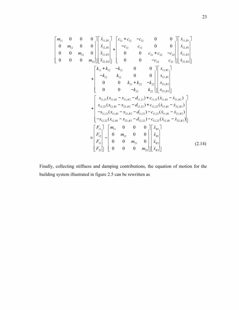
Finally, collecting stiffness and damping contributions, the equation of motion for the
building system illustrated in figure 2.5 can be rewritten as

24
11, 111
12, 112
21, 221
22, 222
11,21 11,2111 12 12
12,22 12,2212 12
11,21 11,2121 22 22
12,22 122 22
0 0 00 0 00 0 00 0 0
0 00 00 00 0
0 00 00 00 0
B
B
B
B
xmxmxmxm
c cc c cc cc c
c cc c cc cc c
+
−+ −
−− + −+ − −−
11, 1
12, 1
21, 2
2,22 22, 2
11,21 11,2111 12 12
12,22 12,2212 12
11,21 11,2121 22 22
12,22 12,2222 22
0 00 00 00 0
0 00 00 00 0
B
B
B
B
xxxx
s sk k ks sk k
s sk k ks sk k
+
−+ − −− + −+ − −−
11, 1
12, 1
21, 2
22, 2
11,21 11,21 11 11
12,22 12,22 12
11,21 11,21 21
12,22 12,22 22
0 0 00
B
B
B
B
xxxx
s d F ms d Fs d Fs d F
− − + = −
1
12 1
21 2
22 2
0 00 0 00 0 0
B
B
B
B
xm x
m xm x
(2.15)
As in the case of single degree of freedom model, for no impact, the following
constraints apply
11, 1 21, 2 11,21 11,21 11,21
12, 1 22, 2 12,22 12,22 12,22
0 , 0
0 , 0
B B
B B
x x d s c
x x d s c
− − ≤ ⇒ =
− − ≤ ⇒ = (2.16)
2.2. BASE ISOLATED BUILDING SYSTEM
2.2.1. SINGLE DEGREE OF FREEDOM SYSTEM
Base isolation system in a building system decreases the inertia force acting on the
superstructure and hence the deflections and shear forces (Arya 1984). A sliding base
isolation system can be provided by using Teflon (TFE) sliding bearings between the
superstructure and its foundation and consists of Teflon-steel interfaces (Mokha et al
25
1990 and Constantinou et al 1990). In actual building a sliding base isolation system
also consists of a centering device or restoring force (Mokha et al 1990) so as to avoid
the residual displacement of the structure, however in the present study this
consideration is neglected. For the sliding isolation system it will be assumed that a
constant coefficient of friction is adequate. In an actual device the static coefficient of
friction is different from the kinetic value and both of these vary as a function of bearing
pressure and sliding velocity (Mokha et al 1990). The coefficient of friction provided
should be chosen according to the expected maximum acceleration peaks in the ground
motion to achieve the maximum advantage of sliding bearing system (Arya 1984).
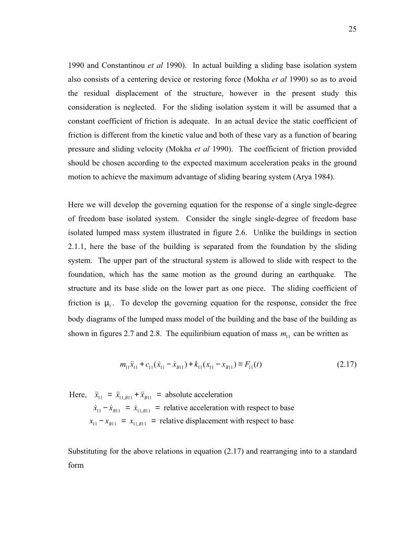
Here we will develop the governing equation for the response of a single single-degree
of freedom base isolated system. Consider the single single-degree of freedom base
isolated lumped mass system illustrated in figure 2.6. Unlike the buildings in section
2.1.1, here the base of the building is separated from the foundation by the sliding
system. The upper part of the structural system is allowed to slide with respect to the
foundation, which has the same motion as the ground during an earthquake. The
structure and its base slide on the lower part as one piece. The sliding coefficient of
friction is 1µ . To develop the governing equation for the response, consider the free
body diagrams of the lumped mass model of the building and the base of the building as
shown in figures 2.7 and 2.8. The equiliribium equation of mass can be written as 11m
11 11 11 11 11 11 11 11 11( ) ( )B Bm x c x x k x x F t+ − + − = ( ) (2.17)
11 11, 11 11
11 11 11, 11
11 11 11, 11
Here, absolute acceleration relative acceleration with respect to base relative displacement with respect
B B
B B
B B
x x xx x x
x x x
= + =− = =
− = = to base
Substituting for the above relations in equation (2.17) and rearranging into to a standard
form

26
10 or B gx xµ1
M B10
M B11
m11
k11, c11
F11
Ground - Inertial Reference Frame
Fig 2.6 Schematic diagram of the single 1-DOF base isolated system
11 ( )F t11 11m x
11 11 11 11 11 11) )( (B Bc x x k x x− −+
Fig 2.7 Free body diagram for lumped mass m11 of the first floor of 1-DOF
base isolated system
11 11, 11 11 11, 11B Bc x k x+
11 11, 10B B BM x
1fF
11 10B BM x
Fig 2.8 Free body diagram for lumped mass MB11 of the base of 1-DOF
base isolated system

27
11 11, 11 11 11, 11 11 11, 11 11 11 11
11 11 11, 10 11 10
( ) ( )
B B B B
B B B
m x c x k x F t m xF t m x m x
+ + = −= − −
(2.18)
The term 11, 10B Bx
11
in above equation is the sliding acceleration, which is the acceleration
of the base of the structure with respect to the foundation. Equiliribium equation for
mass is written from its free body diagram in figure 2.8, assuming the ground
accelerates to the right hand side at the start of earthquake.
BM
11 11, 10 11 11, 11 11 11, 11 1 11 10
11 11 11 11 11, 11 1 11 10
11 11 11, 10 10 11 11, 11 1 11 10
( )
B B B B B f B B
B B f B B
B B B B f B B
M x c x k x F M x
F m x m x F M x
F m x x m x F M x
= + + −
= − − + −
= − + − + −
(2.19)
Simplifying the above equation to obtain
11 11 11, 10 1 11 11 11 10 11 11, 11( ) ( )B B B f B B Bm M x F F m M x m x+ = + − + − (2.20)
The direction of friction force will depend on the velocity of the base of structure
with respect to the foundation and will be in the direction opposite to it. Thus equation
(2.20) can be written in general form as
1fF
11 11 11, 10 11, 10 1 11 11 11 10 11 11, 11( ) sgn( ) ( )B B B B B f B B Bm M x x F F m M x m x+ = − + − + − (2.21)
Here, sgn( )x is the signum function and 1 1 11 11(fF m M= )B gµ + is the constant friction
force during sliding. Dynamic equation for structure and the equation for sliding are
coupled and thus should be solved simultaneously. They are not combined here in a
matrix form since dynamic equation of structure is in the standard form that is
commonly encountered in books. When there is no sliding, equation (2.21) simply

28
becomes . 11, 10 0B Bx =
11 10B BM + −
11 11( )m M
12 12 12m x c
Sliding occurs when the magnitude of the net force acting on the base of the building is
greater then the maximum friction force. At the instant when the sliding starts and
during sliding, the following inequality holds
11 11, 11 11 11, 11 1 11 11( ) (B B f Bx c x k x F m M1− > = µ + (2.22) )g
With some simplifications, it can be rewritten as
10 11 11, 10 11 11, 11 11 11 11(B B B B B Bx m x m x F m M1+ + + − > µ + )g (2.23)
The left hand side of (2.23) is the net force on the base and right hand side is the peak
value of friction force. This inequality can be used to find whether there is sliding, at
any instant. The sliding acceleration 11, 10B Bx in the inequality is non-zero in sliding
phase but is zero at the start of sliding.
2.2.2. TWO DEGREE OF FREEDOM SYSTEM
A two-degree of freedom single building model with base isolation is illustrated in figure
2.9. The corresponding free-body diagrams are given in figures 2.10, 2.11 and 2.12.
The equiliribium equation for mass m12 is
12 11 12 12 11 12( ) ( )x x k x x F t+ − + − = ( ) (2.24)
With simplifications similar as done before, above equation can be rewritten as
12 12, 11 12 12, 11 12 11, 11 12 12, 11 12 11, 11
12 12 11, 10 12 10 ( )B B B B B
B B B
m x c x c x k x k xF t m x m x
+ − + −= − −
(2.25)

29
m12
M B11
M B10
µ1
m11
k11, c11
k12, c12
F12(t)
F11(t)
10 or B gx x
Ground - Inertial Reference Frame
Fig 2.9 Schematic diagram of the single 2-DOF base isolated system
12 ( )F t12 12m x
12 12 11 12 12 11( ) ( )c x x k x x− + −
Fig 2.10 Free body diagram for lumped mass m12 of second floor
12 12 11 12 12 11( ) ( )c x x k x x− + −
11 ( )F t11 11m x
11 11 11 11 11 11( ) ( )B Bc x x k x x− + −
Fig 2.11 Free body diagram for lumped mass m11 of first floor
11 11 11 11 11 11( ) ( )B Bc x x k x x− + −
11 11, 10B B BM x
1fF11 10B BM x
Fig 2.12 Free body diagram for lumped mass MB11 of base

30
Similarly, the equiliribium equation for mass 11m is
11 11 11 11 11 11 11 11 12 12 11 12 12 11 11( ) ( ) ( ) ( )B Bm x c x x k x x c x x k x x F t+ − + − − − − − = ( )
B
=
(2.26)
On simplification, equation (2.26) is written as
11 11, 11 11 11, 11 11 11, 11 12 12, 11 12 11, 11 12 12, 11
12 11, 11 11 11 11, 10 11 10 ( )B B B B B B
B B B
m x c x k x c x c x k xk x F t m x m x
+ + − + −+ = − −
(2.27)
Equations (2.25) and (2.27) can be conveniently written as
11 11, 11 11 12 11, 11 12 12, 11 11 12 11, 11 12 12, 11 11
12 11, 11 12 12, 11 12 11, 11 12 12, 11 1212 12, 11
( ) ( )
B B B B B
B B B BB
m x c c x c x k k x k x Fc x c x k x k x Fm x+ − + −
+ + − + − +
11 11, 10 11 10
12 11, 10 12 10
B B B
B B B
m x m xm x m x
+ − +
(2.28)
Collecting the stiffness and damping contributions, one obtains the following equation
11, 11 11, 11 11, 1111 11 12 12 11 12 12 11
12, 11 12, 11 12, 1112 12 12 12 12 12
00
B B B
B B B
x x xm c c c k k kx x xm c c k k F
+ − + − + + − −
11 1111, 10 10
12 12
0 01 1
0 01 1
F=
B B B
m mx x
m m
− −
(2.29)
Equiliribium equation for the base of the structure as shown in figure 2.12 is
11 11, 10 1 11 11 11 11 11 11 11 10( ) ( )B B B f B B B BM x F c x x k x x M= + − + − − x (2.30)

31
Using equations (2.25) and (2.27) to substitute for in the
above equation and rearranging, we get the equation for sliding acceleration of base of
the structure with respect to the foundation.
11 11 11 11 11 11( ) (B Bc x x k x x− + − )
)B g
11 12 11 11, 10 1 11 12 11 12 11 10
11 11, 11 12 12, 11
( ) ( )
B B B f B B
B B
m m M x F F F m m M x
m x m x
+ + = + + − + +
− − (2.31)
The general equation for sliding can be written by accounting for the direction of friction
force . Rewriting the above equation yields 1fF
11 12 11 11, 10 11, 10 1 11 12
11 12 11 10 11 11, 11 12 12, 11
( ) sgn( )
( )B B B B B f
B B B B
m m M x x F F F
m m M x m x m x
+ + = − + +
− + + − − (2.32)
Where, 1 11 12 11(fF m m M1= µ + + during sliding. Equation (2.32) should be applied
only during sliding. For the case where no sliding occurs, the sliding acceleration is of
course zero. Furthermore, in this case, right hand side of equation (2.31) can be used to
find the actual friction force in the sliding system.
As for the single degree of freedom system, here also sliding will occur when net force
on the base exceeds the friction force. Thus for sliding, the following inequality holds
11 10 11 11 11 11 11 11 1
11 12 11
( ( ) ( ))
( )B B B B f
B
M x c x x k x x F
m m M1
+ − − − − >
= µ + + g (2.33)
With simplifications as done before, the inequality reduces to
11 12 11 10 11 12 11, 10 11 11, 11 12 12, 11 11 12
11 12 11
( ) ( )
( )B B B B B B
B
m m M x m m x m x m x F F
m m M g1
+ + + + + + − −
> µ + +(2.34)

32
When there is no sliding, sliding velocity and acceleration are zero for that building.
2.3. BASE ISOLATION WITH BUILDING POUNDING
2.3.1. SINGLE DEGREE OF FREEDOM SYSTEMS
In the previous sections, formulations were developed separately for pounding and base
isolation. The next objective is to develop the dynamic equation for three single degree
of freedom systems that are base isolated and include pounding considerations as
depicted in figure 2.13.
The dynamic equation for this building system can be written by including impact force
terms in the dynamic equation of the single degree of freedom base isolated system. The
impact force terms couples the three single degree of freedom systems which otherwise
are uncoupled. Note that the displacements and velocities used to calculate the impact
force will be with respect to the lower foundation portion of structure and not the base of
structure, since there will be additional displacement due to sliding.

33
m11
k11, c11
m21
c21,31
m31
k21, c21
k31, c31
s21,31
c11,21
s11,21
d21,31
d11,21
µ1
µ2
µ3
MB11
MB10
MB20
MB21
MB31
MB30
F11 F21
F31
Ground - Inertial Reference Frame
gx (earthquake)
Fig 2.13 Schematic diagram of the three adjacent 1-DOF base isolated systems

34
The equation of motion is
11 11, 11 11 11, 11 11 11, 11
21 21, 21 21 21, 21 21 21, 21
31 31, 31 31 31, 31 31 31, 31
11,21 11, 10 21,
0 0 0 0 0 0
0 0 0 0 0 0
0 0 0 0 0 0
(
B B B
B B B
B B B
B B
m x c x k x
m x c x k x
m x c x k x
s x x
+ + +
−
20 11,21 11,21 11, 10 21, 20
11,21 11, 10 21, 20 11,21 11,21 11, 10 21, 20 21,31 21, 20 31, 30 21,31 21,31 21, 20 31, 30
21,31 21, 20 31, 30 21,31 21,31 21, 2
) ( )
[ ( ) ( )] [ ( ) ( )]
( ) (
B B
B B B B B B B B
B B B
d c x x
s x x d c x x s x x d c x x
s x x d c x
− + −
− − − + − + − − + −
− − − − 0 31, 30
11 11 11, 10 11 10
21 21 21, 20 21
31 31 31, 30 31
)
0 0 0 0
0 0 0 0
0 0 0 0
B
B B B
B B
B B
x
F m x m x
F m x m
F m x m
−
= − −
20
30
B
B
x
x
(2.35)
Collecting the damping and stiffness contributions, one obtains the following matrix
equation
11 11, 11 11 11,21 11,21 11, 11
21 21, 21 21 11,21 11,21 21,31 21,31 21, 21
31 31, 31 31 21,31 21,31 31, 31
0 0 0 0 0
0 0 0 0
0 0 0 0 0
B B
B B
B B
m x c c c x
m x c c c c c x
m x c c c x
k
−
+ + − + −
−
11 11,21 11,21 11, 11 11,21 11,21 11
21 11,21 11,21 21,31 21,31 21, 21 11,21 11,21 21,31 21,31 21
31 21,31 21,31 31, 31 21,31 21,31
0 0 0
0 0
0 0 0
B
B
B
+
s s x s d
k s s s s x s d s d
k s s x s d
− −
+ − + − + − =
−
31
11 11, 10 11 10
21 21, 20 21 20
31 31, 30 31 30
0 0 0 0
0 0 0 0
0 0 0 0
B B B
B B B
B B B
m x m
m x m x
m x m x
− −
F
F
F
x
11,21 11,21 11, 10 11,21 11,21 11, 10
11,21 11,21 21,31 21,31 21, 20 11,21 11,21 21,31 21,31 21, 20
21,31 21,31 31, 30 21,31 21,31 31, 30
0 0
0 0
B B B B
B B B B
B B B B
c c x s s x
c c c c x s s s s x
c c x s s x
− −
− − + − − − + −
− −
(2.36)

35
Equation (2.36) has been written including the impact forces. But at the instant when
there is no pounding, no impact elements are needed and they have to be deactivated in
the solution procedure. To accomplish this, additional constraints must be introduced.
11, 10 21, 20 11,21 11,21 11,21
21, 20 31, 30 21,31 21,31 21,31
0 , 0
0 , 0
B B
B B
x x d s c
x x d s c
− − ≤ ⇒ =
− − ≤ ⇒ = (2.37)
We can also write the equation of motion for sliding of the bases for each of the three
buildings. The equation for Building 1 will be
111 11 11, 10 11, 10 11 11 11 10 11 11, 11( ) sgn( ) ( )B B B B B f B B Bm M x x F F m M x m x+ = − + − + − (2.38)
for Building 2
221 21 21, 20 21, 20 21 21 21 20 21 21, 21( ) sgn( ) ( )B B B B B f B B Bm M x x F F m M x m x+ = − + − + − (2.39)
and for Building 3
331 31 31, 30 31, 30 31 31 31 30 31 31, 31( ) sgn( ) ( )B B B B B f B B Bm M x x F F m M x m x+ = − + − + − (2.40)
Since all the three buildings may not slide at the same time, thus some or all of the above
equations may not be applied at a given time. For any of the buildings during no sliding,
the sliding acceleration and velocity is zero for that building.
The conditions for sliding for each of the three buildings is similar to the one derived
earlier in section 2.2.1. During sliding, following inequalities will hold. In particular,
for Building 1

36
11 11 10 11 11, 10 11 11, 11 11 11 11( ) (B B B B B Bm M x m x m x F m M1+ + + − > µ + )g (2.41)
and for Building 2
21 21 20 21 21, 20 21 21, 21 21 21 21( ) ( )B B B B B Bm M x m x m x F m M2+ + + − > µ + g (2.42)
and for Building 3
31 31 30 31 31, 30 31 31, 31 31 31 31( ) ( )B B B B B Bm M x m x m x F m M3+ + + − > µ + g
B
B
xx
)
(2.43)
2.3.2. TWO DEGREE OF FREEDOM SYSTEMS
In this section the dynamic equations for a two two-degree of freedom building model
with both base isolation and pounding between the buildings is developed. The lumped
mass model of these buildings is illustrated in figure 2.14. The coupled equations of
motion for Building 1 are
11, 11 11, 11 11, 1111 11 12 12 11 12 12
12, 11 12, 11 12, 1112 12 12 12 12
11,21 11, 10 21, 20 11,21 11,21 11, 10 21,
00
( ) (
B B
B B
B B B
x xm c c c k k kx xm c c k k
s x x d c x x
+ − + − + + − −
− − + −+ 20 11
12,22 12, 10 22, 20 12,22 12,22 12, 10 22, 20 12
11, 10 1011 11
11, 10 1012 12
)( ) (
0 0
0 0
B
B B B B
B B B
B B B
Fs x x d c x x F
x xm mx xm m
= − − + −
− −
(2.44)

37
(earthquake)
m12
k12, c12
m11
c11,21
m22
k11, c11
k22, c22
s11,21
c12,22
s12,22
d11,21
d12,22
m21
k21, c21
F11(t)
F21(t)
F22(t)
F12(t)
MB21
MB20
MB10
MB11
µ2
µ1
Ground - Inertial Reference Frame
gx
Fig 2.14 Schematic diagram of the two adjacent 2-DOF base isolated systems

38
and similarly for Building 2
21, 21 21, 21 21, 2121 21 22 22 21 22 22
22, 21 22, 21 22, 2122 22 22 22 22
11,21 11, 10 21, 20 11,21 11,21 11, 10
00
( ) (
B B
B B
B B B
x xm c c c k k kx xm c c k k
s x x d c x x
+ − + − + + − −
− − + −− 21, 20 21
12,22 12, 10 22, 20 12,22 12,22 12, 10 22, 20 22
21, 20 2021 21
21, 20 2022 22
)( ) ( )
0 0
0 0
B
B B B B
B B B
B B B
Fs x x d c x x F
x xm mx xm m
= − − + −
− −
B
B
xx
)B
))
(2.45)
Combining equations (2.44) and (2.45) in to a single matrix equation yields
11, 11 11, 1111 11 12 12
12, 11 12, 1112 12 12
21, 21 21, 2121 21 22 22
22, 21 22, 2122 22 22
11 1
0 0 0 0 00 0 0 0 00 0 0 0 00 0 0 0 0
B B
B B
B B
B B
x xm c c cx xm c cx xm c c cx xm c c
k k
+ − − + + + − −
+ 11, 11 11,21 11, 10 21, 20 11,21 11,21 11, 10 21, 202 12
12, 11 12,22 12, 10 22, 20 12,22 12,22 12, 1012 12
21, 2121 22 22
22, 2122 22
( ) (0 0( ) (0 0
0 00 0
B B B B
B B B B
B
B
x s x x d c x xkx s x x d c x xk kxk k kxk k
− − + −− − − + −− + + − −
22, 20
11,21 11, 10 21, 20 11,21 11,21 11, 10 21, 20
12,22 12, 10 22, 20 12,22 12,22 12, 10 22, 20
11
12
21
22
)( ) (( ) (
B
B B B B
B B B B
s x x d c x xs x x d c x x
FFFF
− − − − − − − − − −
= −
11, 10 1011 11
11, 10 1012 12
21, 20 2021 21
21, 20 2022 22
0 0 0 0 0 00 0 0 0 0 00 0 0 0 0 00 0 0 0 0 0
B B B
B B B
B B B
B B B
x xm mx xm mx xm mx xm m
−
(2.46)
Following the grouping of terms as before, one obtains

39
11, 11 11,21 11,2111 11 12 12
12, 11 12,22 12,2212 12 12
21, 21 11,21 11,2121 21 22 22
22, 21 12,22 12,22 22 22
0 00 0 0 0 0
0 00 0 0 0 0
0 00 0 0 0 0
0 00 0 0 0 0
B
B
B
B
x c cm c c c
x cm c c
x c cm c c c
x cm c c
−+ −
−−+ +
−+ −
−−
11, 11
12, 11
21, 21
22 22, 21
11,21 11,2111 12 12
12,22 12,2212 12
11,21 11,2121 22 22
22 22
0 00 0
0 00 0
0 00 0
00 0
B
B
B
B
x
x
x
x
s sk k k
s sk k
s sk k k
sk k
−+ −
−−+ +
−+ −
−−
c
c
11, 11
12, 11
21, 21
12,22 12,22 22, 21
11,21 11,21 11, 10
12,22 12,22 11, 10
11,21 11,21 21, 20
12,22 12,22
0
0 0
0 0
0 0
0 0
B
B
B
B
B B
B B
B B
x
x
x
s x
c c x
c c x
c c x
c c
−
−+
−
−
11,21 11,21 11, 10
12,22 12,22 11, 10
11,21 11,21 21, 20
21, 20 12,22 12,22 21, 20
11,21 11,21
12,22 12,22
11,21 11,2
0 0
0 0
0 0
0 0
B B
B B
B B
B B B B
s s x
s s x
s s x
x s s x
s d
s d
s d
−
−+
−
−
−
−+
11, 10 1011 11 11
11, 10 1012 12 12
1 21, 20 2021 21 21
12,22 12,22 21, 20 2022 22 22
0 0 0 0 0 0
0 0 0 0 0 0
0 0 0 0 0 0
0 0 0 0 0 0
B B B
B B B
B B B
B B B
x xF m m
x xF m m
x xF m m
s d x xF m m
= − −
(2.47)
and are subject to the following constraints
12, 10 22, 20 12,22 12,22 12,22
11, 10 21, 20 11,21 11,21 11,21
0 , 0
0 , 0
B B
B B
x x d s c
x x d s c
− − ≤ ⇒ =
− − ≤ ⇒ = (2.48)
The dynamic equations for sliding of these structures are similar to equation (2.32) of an
isolated building in section 2.2.2. Thus for Building 1
11 12 11 11, 10 11, 10 1 11 12 11 12 11 10
11 11, 11 12 12, 11
( ) sgn( ) ( )
B B B B B f B B
B B
m m M x x F F F m m M x
m x m x
+ + = − + + − + +
− − (2.49)
and for Building 2

40
21 22 21 21, 20 21, 20 2 21 22 21 22 21 20
21 21, 21 22 22, 21
( ) sgn( ) ( )
B B B B B f B B
B B
m m M x x F F F m m M x
m x m x
+ + = − + + − + +
− − (2.50)
Furthermore, the conditions for sliding of Building 1 is
11 12 11 10 11 12 11, 10 11 11, 11 12 12, 11 11 12
11 12 11
( ) ( )
( )B B B B B B
B
m m M x m m x m x m x F F
m m M1
+ + + + + + − −
> µ + + g (2.51)
and for Building 2 is
21 22 21 20 21 22 21, 20 21 21, 21 22 22, 21 21 22
21 22 21
( ) ( )
( )B B B B B B
B
m m M x m m x m x m x F F
m m M2
+ + + + + + − −
> µ + + g(2.52)
The same argument holds for these inequalities as for other base isolated models
presented previously. The models developed in section 2.3.1 and 2.3.2 are the most
general for single degree and two-degree of freedom systems respectively. By using
appropriate values of coefficient of friction in the sliding isolation system and the
separation between the buildings, we can obtain the models given in other sections.
Moreover it is now possible to investigate the pounding between base isolated and fixed
base buildings that are adjacent to each other. Two separate computer programs have
been written in MATLAB to solve the system of buildings given in section 2.3.1 and
section 2.3.2. These programs have been included in this report and given in Appendix
3 and 4 respectively. Since the models developed in section 2.3 are the most general,
these computer programs can be used to solve the models developed in other sections.

41
3. VALIDATION OF THE NUMERICAL MODEL: FIXED BASE
The dynamic equations derived in sections 2.3.1 and 2.3.2 are the most general and can
be used to analyze other types of adjacent building systems by changing the spacing
between the buildings or by varying the friction coefficient in the base isolation. These
dynamic equations are second order differential equations and can be solved numerically
by converting them into a first order differential equation and then solved using the
ordinary differential equation solvers provided by MATLAB. The first order differential
equation form of these dynamic equations have been given in Appendix 1 and 2 for
single degree and two degree of freedom systems respectively. The MATLAB files
developed for this study are also included and given in Appendix 3 and 4 respectively.
The chapter has been divided into two sections. In the first section, the response of a
single fixed base two degree of freedom building subjected to harmonic base excitation
is obtained analytically using the modal analysis method. The MATLAB code used for
modal analysis is given in Appendix 5. This semi-analytic solution is used to check the
correctness of the response calculated subsequently using numerical technique for which
the MATLAB program is given in Appendix 4. In the second section we will consider
pounding between the fixed base buildings subjected to earthquake ground motion and
analyze the response of this system.
3.1. SEMI-ANALYTIC SOLUTION: 2-DOF BUILDING
Modal analysis method is used to obtain the solution. Modal analysis is used for the
solution of dynamic equation of multi degree of freedom system. In modal analysis as
described in detail in Clough and Penzien (1993), coupled equations of a multi degree of
freedom system are uncoupled using the normal coordinate transformation in equation
(3.1).

42
[ x q= ϕ] (3.1)
Here, x is the geometric coordinate vector and is the generalized coordinate
vector. The matrix [
q
ϕ] is the mode shape matrix. This transformation can be used to
convert the N coupled equations in (3.2) to N uncoupled equations given by (3.3).
[ ] [ ] [ ] ( )m x c x k x p t+ + = (3.2)
2 ( )2 , 1, 2,....,nn n n n n n
n
P tq nM
+ ξ ω +ω = =q q (3.3) N
n
Where, Tn nM m= ϕ ϕ and are generalized mass and load respectively
for the n
( ) ( )Tn nP t p t= ϕ
th mode and nξ and are the critical damping ratio and natural frequency in
that mode. Once generalized coordinates have been obtained from equation (3.3), they
can be used to calculate the response of the system using equation (3.1). The MATLAB
files to obtain the modal analysis solution are given in Appendix 5.
nω

43
2nd floor
1st floor
Foundation
Ground
Fig 3.1 Reference building used for analysis
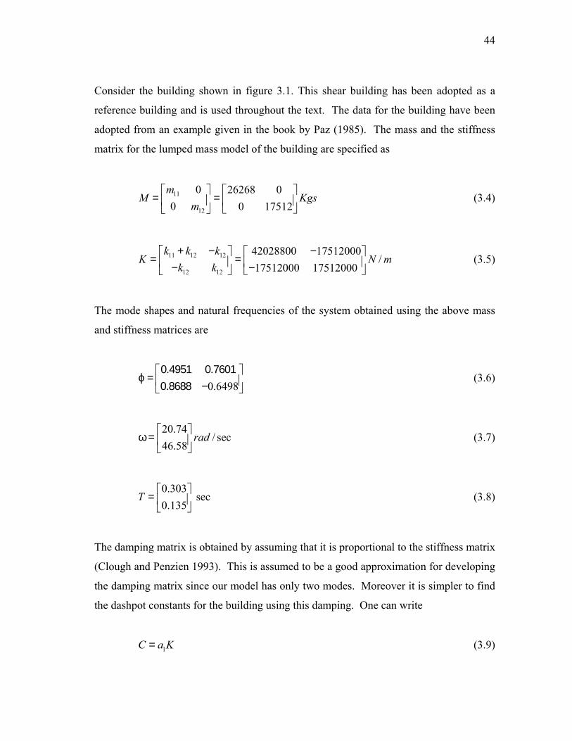
44
Consider the building shown in figure 3.1. This shear building has been adopted as a
reference building and is used throughout the text. The data for the building have been
adopted from an example given in the book by Paz (1985). The mass and the stiffness
matrix for the lumped mass model of the building are specified as
11
12
0 26268 00 0 17512
mM Kgs
m
= =
m
(3.4)
11 12 12
12 12
42028800 17512000/
17512000 17512000k k k
K Nk k+ − −
= = − − (3.5)
The mode shapes and natural frequencies of the system obtained using the above mass
and stiffness matrices are
0.64980.4951 0.7601
ϕ = 0.8688 −
20.74/ sec
46.58rad
ω =
0.303 sec
0.135T
=
(3.6)
(3.7)
(3.8)
The damping matrix is obtained by assuming that it is proportional to the stiffness matrix
(Clough and Penzien 1993). This is assumed to be a good approximation for developing
the damping matrix since our model has only two modes. Moreover it is simpler to find
the dashpot constants for the building using this damping. One can write
1C a K= (3.9)

45
This can be simplified to
1
2n
na ωξ = (3.10)
By assuming 1% damping in the first mode one finds that and this
corresponds to a damping ratio of 2.24% in the second mode. The resulting damping
matrix of the system from (3.9), then is
1 0.000964a =
40515.76 16881.57.sec/
16881.57 16881.57C
−= −
N m (3.11)
This building has been used as the benchmark for all the analysis in this research study.
For the semi-analytic solution, the building is subjected to a sinusoidal earthquake
ground motion. This analysis is done for two different frequencies of the ground
motion. One can write
(3.12) 2 2
sin
Where 10 m/sec , = 2 and 10 rad/sec
g Bx x A t
A
= = Ω
= Ω
Figure 3.2 presents the response of this two-degree of freedom system.

46
0 5 10 15-5-4-3-2-1012345 Second story
Time (sec)
Dis
plac
emen
t (cm
)
Ω = 2 rad/sec2
Ω = 10 rad/sec2
0 5 10 15-5-4-3-2-1012345
First story
Time (sec)
Dis
plac
emen
t (cm
)
Ω = 2 rad/sec2
Ω = 10 rad/sec2
Fig 3.2 Semi-analytical solution for 2-DOF system. Second floor response; First floor response

47
0 5 10 15-5-4-3-2-1012345 Second story
Time (sec)
Dis
plac
emen
t (cm
)
Ω = 2 rad/sec2
Ω = 10 rad/sec2
0 5 10 15-5-4-3-2-1012345
First story
Time (sec)
Dis
plac
emen
t (cm
)
Ω = 2 rad/sec2
Ω = 10 rad/sec2
Fig 3.3 Numerical solution for 2-DOF system. Second floor response; First floor response

48
Numerical solution of the isolated two degree of freedom system subjected to harmonic
ground motion was obtained using the MATLAB file given in Appendix 4 and is
presented in figure 3.3. This response is nearly identical to the semi-analytic solution
one get from modal analysis. Thus the MATLAB program in Appendix 4 is deemed
accurate and will be used in this study. This check however does not confirm the
accuracy of the program when pounding or sliding takes place. The systems in which
pounding or sliding takes place can’t be solved analytically and have to be solved
numerically since these are non-linear behaviors.
3.2. POUNDING IN FIXED BASE BUILDINGS: 2-DOF MODEL
In this research investigation, the focus of the numerical simulation is two degree of
freedom system. Three adjacent building configurations were investigated in the process
of studying building pounding. The first configuration is the common one in which both
the adjacent buildings are fixed base. The second configuration investigates the
pounding between a base isolated and a fixed base building and in the final
configuration, both of the adjacent buildings are base isolated. These configurations
have been illustrated in table 3.1. It also illustrates the section numbers in which these
configurations have been dealt. In this section, response will be calculated for adjacent
buildings whose dynamic equation has been derived in section 2.1.2. The buildings
were modeled as two degree of freedom systems and dynamic equations derived
assuming pounding can take place at any of the floor levels. Buildings have been
subjected to earthquake ground motion with time history of ground acceleration of El
Centro earthquake. Other earthquakes used in this study include those from Mexico
City, Loma Prieta and the Northridge earthquake.
The time history of earthquakes and statistics used to describe them are presented in
figure 3.4 and table 3.2 respectively. It should be noted that the earthquakes have been
arranged in the increasing order of their peak ground acceleration.

49
Table 3.1 Adjacent building configurations used in this study
Building 1 Building 2 Section number
Fixed Fixed: Stiff
Fixed: Flexible 3.2
Base isolated Fixed: Stiff
Fixed: Flexible 4.2
Base isolated Base isolated: Stiff
Base isolated: Flexible4.3

50
0 20 40 60 80 100 120 140 160 180-0.5
0
0.5Mexico City earthquake
a/g
0 5 10 15 20 30 35 40 45 50-0.4
-0.2
0
0.2
0.4El Cent arthquake
a/g
0 5 10 15 25 30 35 40-0.5
0
0.5Loma Pri earthquake
a/g
0 5 10 15 20-1
-0.5
0
0.5
1
Tim (sec)
Northridge earthquake
a/g
ro e
25
eta
20
e
Fig 3.4 Acceleration time histories for the earthquakes

51
Table 3.2 Characterization of environment – Statistics for earthquakes
Earthquake Max Accl. Mean (m/sec2)
Std deviation(m/sec2) Skewness CoE
1985 Mexico City S00E component 0.100 g -0.000080674 0.2135 -0.3805 4.7465
1940 El Centro S00E component 0.340 g 0.00059944 0.4679 0.4476 8.0111
1989 Loma Prieta 0.470 g -0.00038051 0.8266 -0.1113 7.3894
1994 Northridge, taken from pier 10 on the I5 14
ramp C 0.874 g 0.0009669 1.6829 0.0462 5.9197

52
The difference in duration and amplitude are quite evident in figure 3.4. The most
evident statistical characteristic is the coefficient of excess. This clearly shows the non-
gaussian nature of these records.
Adjacent buildings shown in figure 3.5 have been used for analysis. Building 1 is the
reference building described in section 3.1 and Building 2 has a varying stiffness with
respect to the reference building. A stiffer or a more flexible Building 2 is considered
which have mass half or double that of the reference building. Time periods and
frequencies of Building 2 have been depicted in table 3.3. The damping of 1% in the
first mode is kept same as that for the reference building by reconstructing the damping
matrix as its mass is varied. Gap between the buildings have also been varied.
Impact stiffness has been calculated as done by Anagnostopoulos et al 1992 where in the
article it was stated that “the stiffnesses of the impact springs were assigned values such
that the local periods of the mass-impact springs were below the lowest translational
periods of the pounding buildings”. The dashpot constant of the impact element is
calculated using these formulas (Anagnostopoulos 1988).
1 22
1 2
ln2 and (ln )
i ikm m rc
m m rπ−= ξ ξ =
+ + 2 (3.13)
Here, is the stiffness of the impact element and ξk i is the damping ratio and depends on
the coefficient of restitution between the colliding masses for the inelastic impact, r is
the coefficient of restitution whose value is 1 for completely elastic impact and 0 for
completely plastic impact. Since pounding of buildings is neither fully elastic nor fully
plastic, we can assume its value to be 0.50 as done by Anagnostopoulos et al 1992.

53
Building 1
Building 2
2nd floor
1st floor
Foundation
Base of structure
Fixed
Fig 3.5 Adjacent fixed base buildings
Table 3.3 Properties of Building 2
Building 2
Properties Stiff Flexible
Mass with respect to reference building Half Twice
First mode time period (sec) 0.2142 0.4284
Second mode time period (sec) 0.0954 0.1908
First mode frequency (rad/sec) 29.33 14.66
Second mode frequency (rad/sec) 65.87 32.94

54
In this section the response of the buildings studied in section 2.1.2 have been
investigated for El Centro earthquake. It was found from response time history that the
impact between the lower floors is very less. Hence all the analysis and any reference to
displacement response of building in this study refer to top floor responses.
Figure 3.6 shows response time history of Building 1 and also the impact forces during
pounding for the case when buildings are spaced 2 cm apart and Building 2 is flexible.
Asterisk on the time history response indicates pounding at that time. Figure 3.7 shows
the variation in number of impacts with increase in gap between the buildings for
different stiffness of Building 2. It can be seen from this graph that number of total
impacts decreases with increase in gap and it decreases faster in case when Building 2 is
stiff. Also the total number of impacts is higher when Building 2 is flexible as compared
to the case when it is stiff. In both of these cases the number of in-phase is lower than
out of phase impacts. In-phase impacts are those that occur while the buildings are
moving in the same direction and out of phase impacts are those that occur while they
move in the opposite direction and towards each other. It is expected that out of phase
impacts decreases the response of the pounding buildings but can cause more local
damage whereas in-phase impacts increases the response but cause less local damage.

55
0 5 10 15 20 25 30 35 40 45 50-5
-4
-3
-2
-1
0
1
2
3
4
5
Time (sec)
Dis
plac
emen
t (cm
)
Displacement responsePounding locations
0 5 10 15 20 25 30 35 40 45 500
100
200
300
400
Time (sec)
Impa
ct fo
rce
(KN
)
Fig 3.6 Response time history of Building 1; Impact forces; Building 2: Flexible, Gap = 2 cm

56
Total, in-phase and out of phase impacts of Building 1
0
10
20
30
40
50
60
70
80
90
100
0 1 2 3 4 5 6 7 8
Gap (cm)
Num
ber o
f im
pact
s
Building 2 Stiff:Total impacts
Building 2 Stiff: In-phase impacts
Building 2 Stiff:Out of phaseimpactsBuilding 2 Flexible:Total impacts
Building 2 Flexible:In-phase impacts
Building 2 Flexible:Out of phaseimpacts
Fig 3.7 Variation in number of impacts with increasing gap between the buildings

57
Magnitude of peak displacement of Building 1
00.5
11.5
22.5
33.5
44.5
5
0 1 2 3 4 5 6 7 8
Gap (cm)
Peak
Dis
plac
emen
t (cm
)
Building 2: Stiff
Building 2:Flexible
Fig 3.8 Variation of peak displacement with increasing gap between the buildings
Peak magnitude of impact force on Building 1
0
100
200
300
400
500
0 1 2 3 4 5 6 7 8
Gap (cm)
Impa
ct fo
rce
(KN
)
Building 2: StiffBuilding 2: Flexible
Fig 3.9 Variation in peak impact force with increasing gap between the buildings

58
Figure 3.8 and 3.9 shows the variation in magnitude of peak displacement and peak
impact force as the gap between the buildings is varied. It was observed that peak
displacement decreased with increase in pounding when the gap is reduced, probably
due to more out of phase impacts. Also peak displacement was found to increase as the
gap size is reduced to a very small distance (although the overall response was found to
be less), probably due to very high amount of pounding in which there can be lot of in-
phase impacts. This peak displacement was higher when Building 2 is flexible. This is
in compliance with the study done by Anagnostopoulos 1988, who reached the same
conclusion for fixed base buildings with very small gap. The maximum impact force
was found to be higher in flexible building case than the stiff building case and in both
the cases it reduced with increase in the gap.

59
4. SIMULATION OF BUIILDING POUNDING WITH BASE ISOLATION
The numerical results presented in this chapter were obtained using the MATLAB
program given in Appendix 4. This chapter is divided into three sections. The first
section deals with calculating the response of single base isolated building for a selected
range of friction coefficient values. Four different earthquakes that cover a range of
magnitudes are used in the building response simulation. In the second section the
response of two adjacent buildings, one of which is base isolated and the other one
having fixed base, is simulated. We will assume that Building 1 is base isolated and is
the reference building. In the third section, response of two adjacent buildings, both of
them being base isolated, is obtained.
4.1. SINGLE BASE ISOLATED BUILDING
In this section the response behavior of single base isolated two degree of freedom
building is investigated. The reference building described earlier is now used and this
provides a basis for later simulations. Here, mass of the building base is assumed to be
half the mass of the lumped first floor. The response has been calculated for many
coefficients of friction to examine the variation in response behavior. Figure 4.1 and 4.2
shows the variation of skewness and coefficient of excess for the total displacement
response of second floor for the base isolated building subjected to different earthquakes.
From these figures it can be seen that skewness and coefficient of excess for Mexico
City earthquake is constant, since there is no sliding of the building at any time. Further,
the skewness is very small and coefficient of excess is high due to low intensity of the
earthquake. For the other earthquakes it can be seen that skewness first decreases and
then increases as the friction coefficient increases. Coefficient of excess for these
earthquakes tends towards one with an increase in friction coefficient.

60
-1.5
-1
-0.5
0
0.5
1
1.5
0 0.1 0.2 0.3 0.4
Coefficient of friction
Skew
ness
Mexico CityEl CentroLoma PrietaNorthridge
Fig 4.1 Skewness of total displacement response for different earthquakes
-3
-2
-1
0
1
2
3
4
5
6
0 0.1 0.2 0.3 0.4
Coefficient of friction
Coe
ffici
ent o
f Exc
ess
Mexico CityEl CentroLoma PrietaNorthridge
Fig 4.2 Coefficient of excess of total displacement response for different earthquakes

61
Variation of maximum relative displacement, maximum sliding displacement and
maximum total displacement with coefficient of friction for different earthquakes have
been given in figures 4.3, 4.4 and 4.5 respectively. With regards to the building sliding
response, the Northridge case is the most dramatic as the response decrease significantly
with increase in the friction coefficient. Since sliding displacement response is usually
much higher than the relative displacement response, the variation in total displacement
response is approximately same as that of sliding displacement for each of the
earthquakes. One is surprised to note that sliding displacement have increased with
increase in friction coefficient for Loma Prieta earthquake, which otherwise will be
expected to decrease. The relative displacement response is lower for lower coefficients
of friction as expected, which illustrates the advantage of base isolation of buildings.
Since there is an upper limit on the shear force that can be transferred by the sliding
interface to the superstructure, it can be seen that the relative displacement responses are
approximately same for the three earthquakes of different intensities. Thus a base
isolation system proves to be most useful for higher intensity earthquakes.
A series of histograms superimposed with a corresponding normal distribution curve for
identical buildings with a specified coefficient of friction in the base isolation system are
presented in figure 4.6. Intrestingly it is observed that Loma Prieta is the only
earthquake for which the mean is on the negative side. It is not obvious as to why this
occurs. Finally it was intresting to observe that only Mexico City earthquake resulted in
a building response whose mean was close to zero.

62
0
0.5
1
1.5
2
2.5
3
0 0.1 0.2 0.3 0.4
Coefficient of friction
Max
imum
rela
tive
disp
lace
men
t (c
m)
Mexico CityEl CentroLoma PrietaNorthridge
Fig 4.3 Maximum relative displacement response for different earthquakes
0
5
10
15
20
25
30
35
40
45
0 0.1 0.2 0.3 0.4
Coefficient of friction
Max
imum
slid
ing
disp
lace
men
t (cm
)
Mexico CityEl CentroLoma PrietaNorthridge
Fig 4.4 Maximum sliding displacement response for different earthquakes

63
0
5
10
15
20
25
30
35
40
45
0 0.1 0.2 0.3 0.4
Coefficient of friction
Max
imum
tota
l dis
plac
emen
t (cm
)
Mexico CityEl CentroLoma PrietaNorthridge
Fig 4.5 Maximum total displacement response for different earthquakes

64
-2 -1 0 1 2
Displacement (cm)
Pro
babi
lity
Mexico city earthquake , µ = 0.2
-6 -4 -2 0 2 4 6
Displacement (cm)P
roba
bilit
y
El Centro earthquake , µ = 0.2
-6 -4 -2 0 2 4 6
Displacement (cm)
Pro
babi
lity
Loma Prieta earthquake , µ = 0.2
-10 -5 0 5 10
Displacement (cm)
Pro
babi
lity
Northridge earthquake , µ = 0.2
Fig 4.6 Histograms and normal probability curve for the displacement response of base isolated
reference building subjected to different earthquakes

65
4.2. FIXED BASE AND BASE ISOLATED ADJACENT BUILDINGS
This section considers the response of a base isolated building that is closely placed to a
fixed base building. The buildings are illustrated in figure 4.7 and it is assumed that
Building 1 is the reference building and is base isolated. For the response simulations,
Building 2 is either stiffer or more flexible than the reference building. In this study, the
building system has been subjected to ground acceleration corresponding to the four
selected earthquakes. Although the friction coefficient in base isolation will practically
range from 0.05 to 0.2, simulations have been done and results presented for higher
values also in order to see the response behavior.
The total number of impacts for different stiffness of Building 2 and for different friction
coefficient in the sliding system of Building 1 is presented in figure 4.8. It can be seen
that the total numbers of impacts were higher for stiffer version of Building 2 when
coefficient of friction is low whereas they were higher for more flexible version of
Building 2 when coefficient of friction is high. This occured since during El Centro
earthquake, when friction coefficient is low, Building 1 was observed to slide towards
Building 2 thus decreasing the gap between the buildings. Note that as the gap reduces,
the impacts for stiffer system increase faster.

66
Building 1
Building 2
Sliding material
2nd Storey
1st Storey
Foundation
(Base isolation)
Base of structure
Fixed
Fig 4.7 Adjacent base isolated and fixed base buildings

67
Building 1: Base isolated
0
20
40
60
80
100
120
0.1 0.2 0.3 0.4 0.5 ∞Coefficient of fricton
Tota
l num
ber o
f im
pact
s
Building 2: StiffBuilding 2: Flexible
Fig 4.8 Total number of impacts as a function of Building 2 stiffness and base isolation friction
coefficient in Building 1
Building 1: Base isolated
050
100150200250300350400450
0.1 0.2 0.3 0.4 0.5 ∞Coefficient of friction
Max
imum
Impa
ct fo
rce
(KN
) Building 2: StiffBuilding 2: Flexible
Fig 4.9 Maximum impact force as a function of Building 2 stiffness and base isolation friction
coefficient in Building 1

68
Figure 4.9 shows the variation of maximum impact force and figure 4.10 presents the
maximum duration of impacts. It was found that the impact force and duration of
impacts was higher when Building 2 was flexible. For coefficient of friction equal to 0.3
and 0.4 when Building 2 is stiff, it was observed that there are some impacts with
relatively high durations. From response time histories it was observed that in these
cases Building 1 slid very close to Building 2. Due to decrease in gap, they acted as if
sticking to each other and more so when friction coefficient was 0.4. Due to this, the
impact duration was very high and it has not been shown in figure 4.10. This did not
happen when Building 2 was flexible, since high magnitude of impact caused sliding and
shifted Building 1 away from it, again increasing the gap between them. Figure 4.11
presents information on the nature of the maximum magnitude of total displacement for
second floor of Building 1. Note that the total displacement is measured with respect to
the original location of the building. It was observed from the time histories of response
that when Building 2 is flexible, the impact force was very high that caused the sliding
of Building 1 in opposite direction resulting in a high sliding displacement. Whereas
when Building 2 is stiff, lower impact forces do not cause much sliding. A higher total
displacement in the mid-value range of friction coefficient was due to higher relative
displacement that occurred for higher friction coefficient in addition to sliding
displacement.
Table 4.1 presents some of the statistics for total displacement for varying friction
coefficients in the base isolation system of Building 1 and stiff Building 2 with a gap
between them equal to 2 centimeters. Table 4.2 shows the same statistics for different
earthquakes and friction coefficient equal to 0.2. In case of Loma Prieta and Northridge
earthquakes, very high and impractical sliding displacements due to pounding were
observed at a gap of 2 centimeters. Thus the gap between the buildings, when subjected
to these earthquakes, was increased to 4 and 8 centimeters respectively.

69
Building 1: Base isolated
00.010.020.030.040.050.060.070.080.09
0.1 0.2 0.3 0.4 0.5 ∞Coefficient of friction
Max
imum
dur
atio
n of
im
pact
s (s
ec)
Building 2: StiffBuilding 2: Flexible
Fig 4.10 Maximum duration of impacts as a function of Building 2 stiffness and base isolation
friction coefficient in Building 1
Building 1: Base isolated
012345678
0.1 0.2 0.3 0.4 0.5 ∞Coefficient of friction
Max
imum
of m
agni
tude
of
tota
l dis
plac
emen
t (cm
)
Building 2: StiffBuilding 2: Flexible
Fig 4.11 Total displacement as a function of Building 2 stiffness and base isolation friction coefficient
in Building 1

70
Table 4.1 Response behavior characterization for varying friction coefficients. Building 1: base
isolated, Building 2: stiff
Adjacent buildings with stiff Building 2
Friction coefficients for base isolated Building 1 Statistics
Single reference
building, fixed base
µ = ∞ µ = 0.5 µ = 0.4 µ = 0.3 µ = 0.2 µ = 0.1
Mean (cm) 0 -0.0021 0.77 2.11 -0.0067 0.71 0.36 Variance (cm) 0.49 0.4356 0.3364 0.8464 0.7921 0.3025 0.1936
Std deviation (cm) 0.7 0.66 0.58 0.92 0.89 0.55 0.44 Skewness 0.0246 -0.0107 -0.5361 -1.4938 0.8739 -0.3464 -0.4364
CoE 1.8417 0.9556 1.229 2.2515 1.5333 0.9919 2.3687Total number of
impacts NA 8 32 109 40 24 10
Table 4.2 Response behavior characterization for earthquakes of increasing intensity. Building 1:
base isolated, Building 2: stiff
Friction coefficient µ = 0.2 , Gap = 2 cm
Earthquake Mean (cm) Std deviation (cm) Skewness CoE Inphase
impacts Out of phase
impacts Mexico City 0 0.07486 0.1465 4.7465 0 0 El Centro 0.71 0.55 -0.3464 0.9919 6 18
Loma Prieta, Gap = 4 cm -2.05 1.06 1.2448 0.6232 0 0
Northridge, Gap = 8 cm 2.36 2.58 -0.9539 2.4053 0 4

71
Table 4.3 Response behavior characterization for varying friction coefficients. Building 1: base
isolated, Building 2: flexible
Adjacent buildings with flexible Building 2
Friction coefficients for base isolated Building 1 Statistics
Single reference
building, fixed base
µ = ∞ µ = 0.5 µ = 0.4 µ = 0.3 µ = 0.2 µ = 0.1
Mean (cm) 0 -0.027 0.5 -3.18 -0.172 -1.43 -1.45 Variance (cm) 0.49 0.16 0.2809 1.6384 0.5625 0.3844 0.2601
Std deviation (cm) 0.7 0.4 0.53 1.28 0.75 0.62 0.51 Skewness 0.0246 -0.1577 -1.111 1.6341 0.7415 0.192 1.0417
CoE 1.8417 2.8934 5.6526 3.2429 2.9527 1.9298 5.7851Total number of
impacts NA 38 57 9 7 5 4
Table 4.4 Response behavior characterization for earthquakes of increasing intensity. Building 1:
base isolated, Building 2: flexible
Friction coefficient µ = 0.2 , Gap = 2 cm
Earthquake Mean (cm) Std deviation (cm) Skewness CoE Inphase
impacts Out of phase
impacts Mexico City 0 0.07486 0.1465 4.7465 0 0 El Centro -1.43 0.62 0.192 1.9298 2 3
Loma Prieta, Gap = 4 cm -6.51 3.13 1.448 0.6515 4 4
Northridge, Gap = 8 cm -9.53 7.8 0.3587 -1.7383 2 3

72
Table 4.3 and 4.4 are the corresponding tables when Building 2 is flexible. Comparing
the mean of response in tables 4.2 and 4.4, it can be seen that the means shifts to left side
or the negative side when Building 2 is flexible. This happens since the impact force for
flexible building is large which causes large sliding displacements of Building 1. A
similar phenomenon can be observed in table 4.1 and 4.3 where the buildings are
subjected to El Centro earthquake and result have been presented for various values of
coefficient of friction. It can also be observed in tables 4.2 and 4.4 that when the mean
is positive, skewness is negative and vice versa. This happens due to peak in the
distribution of response at the original position of the building that is at zero.
4.3. BASE ISOLATION IN BOTH ADJACENT BUILDINGS
The response behavior of two adjacent base isolated buildings is presented in this
section. The system of buildings is same as shown in figure 4.7 except that here
Building 2 is base isolated as well. It is assumed that the friction coefficient in the base
isolation system of both the buildings is the same. As done in the last section, here also
we will draw bar graphs for total number of impacts, maximum impact force, maximum
duration of impacts and maximum of the magnitude of total displacements. These
graphs have been given in figures 4.12, 4.13, 4.14 and 4.15 respectively. As previously
shown, here also the total number of impacts is higher for stiffer Building 2 when the
friction coefficient of sliding system is small and is higher for more flexible Building 2
when friction coefficient is large. An exception to this was seen for coefficient of
friction equal to 0.1. In this case it was found that since friction coefficient is small,
both the buildings slides and keep the distance between them approximately same. Thus
there is very less pounding for a stiff Building 2 case. Maximum impact force and the
maximum duration of impacts, as seen earlier, are generally higher when Building 2 is
flexible. The maximum of the magnitude of total displacement is observed to reduce
considerably for flexible Building 2 as seen in figure 4.15 as compared to figure 4.11
where only Building 1 was base isolated.

73
Both buildings: Base isolated
0
10
20
30
40
50
0.1 0.2 0.3 0.4 0.5 ∞Coefficient of friction
Tota
l num
ber o
f im
pact
s
Building 2: StiffBuilding 2: Flexible
Fig 4.12 Total number of impacts as a function of Building 2 stiffness and base isolation friction
coefficient
Both buildings: Base isolated
0
200
400
600
800
1000
1200
0.1 0.2 0.3 0.4 0.5 ∞Coefficient of friction
Max
imum
Impa
ct fo
rce
(KN
) Building 2: StiffBuilding 2: Flexible
Fig 4.13 Maximum impact force as a function of Building 2 stiffness and base isolation friction
coefficient

74
Both buildings: Base isolated
00.010.020.030.040.050.060.070.08
0.1 0.2 0.3 0.4 0.5 ∞Coefficient of friction
Max
imum
dur
atio
n of
im
pact
s (s
ec)
Building 2: StiffBuilding 2: Flexible
Fig 4.14 Maximum duration of impacts as a function of Building 2 stiffness and base isolation
friction coefficient
Both buildings: Base isolated
0
5
10
15
20
0.1 0.2 0.3 0.4 0.5 ∞Coefficient of friction
Max
imum
of t
he
mag
nitu
de o
f tot
al
disp
lace
men
t (cm
)
Building 2: StiffBuilding 2: Flexible
Fig 4.15 Maximum total displacement as a function of Building 2 stiffness and base isolation friction
coefficient

75
Building 2: Stiff
00.5
11.5
22.5
33.5
0.1 0.2 0.3 0.4 0.5 ∞Coefficient of friction
Max
imum
of m
agni
tude
of
rela
tive
disp
lace
men
t (cm
)
Building 1: Base isolated
Both buildings: Baseisolated
Fig 4.16 Maximum relative displacement as a function of base isolation friction coefficient with stiff
Building 2
Building 2: Flexible
0
2
4
6
8
10
0.1 0.2 0.3 0.4 0.5 ∞Coefficient of friction
Max
imum
of m
agni
tude
of
rela
tive
disp
lace
men
t (cm
)
Building 1: Base isolated
Both buildings: Baseisolated
Fig 4.17 Maximum relative displacement as a function of base isolation friction coefficient with
flexible Building 2

76
Bar graphs for relative displacements of second floor of Building 1 for El Centro
earthquake have been given in figures 4.16 and 4.17. Note that the relative displacement
is the displacement of a building with respect to its base and does not include the sliding
displacement. It can be seen from these graphs that as expected the relative
displacements decreased with decrease in coefficient of friction or increase in sliding.
From figure 4.16, it can be seen that there is not much difference in response between
single base isolated and both base isolated cases for stiff Building 2 but the response is
considerably less for both base isolated case when Building 2 is flexible as is visible
from figure 4.17. In the later case the response again starts decreasing, since, with
increase in coefficient of friction, sliding decreases, which increases the relative
response and increases the pounding. This pounding decreases the response of the
system.
Table 4.5 shows some of the statistics for total displacement with varying friction
coefficients in the base isolation system and stiff Building 2. The gap between the
adjacent buildings is equal to 2 centimeters. Table 4.6 shows the same statistics for
different earthquakes and when friction coefficient equal to 0.2. Here also the gap
between the buildings is kept 4 cm and 8 cm respectively when subjected to Loma Prieta
and Northridge earthquakes. Table 4.7 and 4.8 are the corresponding tables when
Building 2 is flexible. Comparing the means of response in tables 4.6 and 4.8, it can be
seen that there is not much difference in the values. This happens since both the
buildings can slide in this case keeping the gap between them approximately constant. It
was observed that in this case no pounding took place for Northridge earthquake and
very little for Loma Prieta earthquake. For El Centro earthquake, some pounding took
place but the impact force was not large enough to cause sliding. A similar phenomenon
can be observed in table 4.5 and 4.7 where the buildings are subjected to El Centro
earthquake.

77
Table 4.5 Response behavior characterization for varying friction coefficients. Both buildings: base
isolated, Building 2: stiff
Adjacent buildings with stiff Building 2
Friction coefficients for both base isolated buildings Statistics
Single reference
building, fixed base
µ = ∞ µ = 0.5 µ = 0.4 µ = 0.3 µ = 0.2 µ = 0.1
Mean (cm) 0 -0.0021 0.46 -0.033 0.88 0.64 0.58 Variance (cm) 0.49 0.4356 0.3721 0.3721 0.3844 0.2809 0.2025
Std deviation (cm) 0.7 0.66 0.61 0.61 0.62 0.53 0.45 Skewness 0.0246 -0.0107 -0.2036 0.1803 -0.9856 -0.2221 -1.2491
CoE 1.8417 0.9556 0.7537 0.5925 1.0621 0.9919 2.7623 Total number of
impacts NA 8 16 4 22 18 1
Table 4.6 Response behavior characterization for earthquakes of increasing intensity. Both
buildings: base isolated, Building 2: stiff
Friction coefficeint µ = 0.2 , Gap = 2 cm
Earthquake Mean (cm)
Std deviation (cm) Skewness CoE Inphase
impacts Out of phase
impacts Mexico City 0 0.07486 0.1465 4.7465 0 0 El Centro 0.64 0.53 -0.2221 0.9919 4 14
Loma Prieta, Gap = 4 cm -2.05 1.06 1.2448 0.6232 0 0
Northridge, Gap = 8 cm 2.95 2.99 -0.8068 0.925 0 0

78
Table 4.7 Response behavior characterization for varying friction coefficients. Both buildings: base
isolated, Building 2: flexible
Adjacent buildings with flexible Building 2
Friction coefficients for both base isolated buildings Statistics
Single reference
building, fixed base
µ = ∞ µ = 0.5 µ = 0.4 µ = 0.3 µ = 0.2 µ = 0.1
Mean (cm) 0 -0.027 1.62 -8.55 -0.17 0.26 0.47 Variance (cm) 0.49 0.16 0.6889 20.25 0.3481 0.2809 0.1681
Std deviation (cm) 0.7 0.4 0.83 4.5 0.59 0.53 0.41 Skewness 0.0246 -0.1577 -1.9928 1.31 0.6325 0.0264 -0.5834
CoE 1.8417 2.8934 6.1115 -0.1012 1.0328 0.1762 2.4457 Total number of
impacts NA 38 47 20 15 2 3
Table 4.8 Response behavior characterization for earthquakes of increasing intensity. Both
buildings: base isolated, Building 2: flexible
Friction coefficient µ = 0.2, Gap = 2 cm
Earthquake Mean (cm) Std deviation (cm) Skewness CoE Inphase
impacts Out of phase
impacts Mexico City 0 0.07486 0.1465 4.7465 0 0 El Centro 0.26 0.53 0.0264 0.1762 0 2
Loma Prieta, Gap = 4 cm -1.86 0.95 1.305 1.0618 0 2
Northridge, Gap = 8 cm 3.01 3.02 -0.7647 0.7906 0 0

79
Figure 4.18 presents four histograms and normal probability plots of total displacement
response of second floor of Building 1 for adjacent buildings subjected to El Centro
earthquake. It can be seen that with a stiff Building 2 and base isolated Building 1, the
mean is on the positive side but when Building 2 is flexible, the mean shifts to negative
since pounding with the flexible building caused large sliding displacements in negative
direction. In this case if flexible Building 2 is also base isolated, then it can be seen that
the mean again shifts to positive side since there is considerable reduction in response of
the flexible building due to base isolation which in turn reduces pounding. Thus in case
of flexible Building 2, response is governed by pounding since impact force is high. For
stiff Building 2, if both the buildings are base isolated, then there is not a considerable
change in response since the response is dominated by earthquake, as the impact force of
pounding is very low.
Similar discussion holds for adjacent buildings whose response histograms are shown in
figure 4.19. Here the buildings are subjected to Loma Prieta earthquake, which is a
considerably different earthquake than El Centro earthquake as shown in section 4.1. In
this case also the sliding displacement of Building 1 is considerably reduced when
Building 2 is made base isolated. This phenomenon is also well reflected from the time
histories of the response given in figure 4.20. Thus the worst case can be seen as the one
when base isolated building is close to fixed base building and one or both of them are
flexible. In this case the impact forces are large and pounding if occurs can cause lot of
sliding displacements in addition to local damage.

80
-4 -3 -2 -1 0 1 2 3 4Displacement (cm)
Pro
babi
lity
Building 2: Stiff , Building 1: Base isolated µ = 0.2
-4 -3 -2 -1 0 1 2 3 4Displacement (cm)
Pro
babi
lity
Building 2: Flexible , Building 1: Base isolated µ = 0.2
-4 -3 -2 -1 0 1 2 3 4Displacement (cm)
Pro
babi
lity
Building 2: Flexible , Both Buildings: Base isolated µ = 0.2
-4 -3 -2 -1 0 1 2 3 4Displacement (cm)
Pro
babi
lity
Building 2: Stiff , Both buildings: Base isolated µ = 0.2
Fig 4.18 Histogram and normal probability density function of total displacement for El Centro
earthquake, Gap = 2 cm

81
-6 -4 -2 0 2 4 6Displacement (cm)
Pro
babi
lity
Building 2: Stiff , Building 1: Base isolated µ = 0.2
-20 -15 -10 -5 0 5Displacement (cm)
Pro
babi
lity
Building 2: Flexible , Building 1: Base isolated µ = 0.2
-6 -4 -2 0 2 4 6Displacement (cm)
Pro
babi
lity
Building 2: Flexible , Both Buildings: Base isolated µ = 0.2
-6 -4 -2 0 2 4 6Displacement (cm)
Pro
babi
lity
Building 2: Stiff , Both buildings: Base isolated µ = 0.2
Fig 4.19 Histogram and normal probability density function of total displacement for Loma Prieta
earthquake, Gap = 4 cm

82
0 5 10 15 20 25 30 35 40 45 50
-4
-2
0
2
4
Dis
plac
emen
t (cm
)
0 5 10 15 20 25 30 35 40 45 50
-4
-2
0
2
4
Dis
plac
emen
t (cm
)
0 5 10 15 20 25 30 35 40 45 50
-4
-2
0
2
4
Time (sec)
Dis
plac
emen
t (cm
)
Building 1: Base isolated , Building 2: Fixed , Stiff
Building 1: Base isol ed , Building 2: Fixed , Flexible
Both buildings: Base isolated , Building 2: Flexible
at
Fig 4.20 Time histories of total displacement for El Centro earthquake, µ = 0.2, Gap = 2 cm

83
The correlation coefficients of the displacement response of Building 1 for various cases
of base isolation and for stiff Building 2 to single fixed building response are presented
in table 4.9 and table 4.10 shows the corresponding correlation coefficients for flexible
Building 2. It can be observed that for fixed-fixed case, correlation coefficients are
lower for flexible Building 2, since there is more pounding in flexible buildings as
discussed earlier. Since both pounding and sliding are non-linear phenomenon, the
correlation coefficients are very small. Correlation between the responses decreases
when pounding is introduced and further decreases as base isolation effect is increased.
Due to little correlation between the responses, it was earlier found difficult to anticipate
the variation of parameters like number of impact, their magnitude, in-phase and out of
phase impacts, duration of impacts, maximum total sliding displacement, relative
displacement, sliding displacement, residual sliding displacements and statistical
parameters discussed earlier, as a function of coefficient of friction in base isolation.
In this study no centering force was considered in the base isolation system and also
there is no limit on the maximum sliding displacement. In an actual base isolation
system there will be a limit on the maximum sliding displacement. Also the friction
pendulum system that is a more commonly used for friction bearing base isolation will
also have a centering force. Adding a maximum limit on sliding would have added
another non-linear effect and would have made the response more unpredictable and
difficult to interpret. Both of these factors tend to maintain gap between the buildings
thus reducing the chances of pounding, which occurred in our simulations.

84
Table 4.9 Correlation coefficients, Building 2: stiff
µ Fixed-Base isolated
Base isolated-Base isolated
Fixed – Fixed, µ = ∞ 0.9529 0.9529
0.3 0.0661 0.3404 0.2 -0.0548 -0.0137 0.1 0.0378 0.027
Table 4.10 Correlation coefficients, Building 2: flexible
µ Fixed-Base isolated
Base isolated-Base isolated
Fixed – Fixed, µ = ∞ 0.4468 0.4468
0.3 0.2208 0.4476 0.2 0.0257 -0.0156 0.1 0.0161 0.0064

85
5. SUMMARY AND CONCLUSION
5.1. SUMMARY AND SCOPE OF STUDY
In this research investigation, adjacent buildings were modeled as lumped mass systems
with impact taking place only at floor levels. Inelastic impacts were taken into account
by utilizing linear elastic spring and dashpots at the floor level where the impact occurs,
as was suggested earlier by Anagnostopoulos and Spiliopoulos (1992). Base isolation for
each building was simulated by allowing the building to slide along a horizontal
frictional plane at a specified foundation elevation (Mostaghel and Tanbakuchi 1983).
The base isolation system adopted in this study is flat sliding surface type and no
centering force acts at any time nor is there a limit on the maximum sliding displacement
by the buildings. Of course for actual systems both of these considerations must be
addressed. Friction coefficients between the sliding surfaces have also been assumed
constant which otherwise would vary in practice. Inelastic behavior and any rotational
affects of the buildings have been neglected.
The dynamic response equations written for each building include effects of sliding and
building impact. The resulting systems of second order constant coefficient equations
are recast as a system of first order ordinary differential equations and solved using
‘MATLAB’ ode solvers. The external loading on the structures includes actual
acceleration time histories from earthquakes in California and Mexico. The equations
were formulated so that the adjacent structures can have different foundations (fixed or
base isolated) and can be subjected to different ground motions. In this analysis,
buildings are modeled as shear buildings and do not include frame behavior. Further,
damage caused by building impacts has not been taken into account and this can make
the model prediction unrealistic. The spacing between the buildings in some cases was
kept small in order to study pounding and impact. Although current design codes call
for larger spacing between base isolated buildings, in some cases like historic restoration

86
and seismic rehabilitation of old fixed base buildings using base isolation systems, the
gap may indeed become quite small.
In this research investigation, the focus of the numerical simulation is two degree of
freedom system. Three adjacent building configurations were investigated in the process
of studying building pounding. The first configuration is the common one in which both
the adjacent buildings are fixed base. The second configuration investigates the
pounding between a base isolated and a fixed base building and in the final
configuration, both of the adjacent buildings are base isolated. Pounding between the
floors of adjacent buildings can occur when the buildings vibrate in modes that are not
completely in-phase. Building pounding can influence the response of the colliding
buildings and can cause local damage at the locations where impact takes place. For
base isolated building systems, pounding behavior can be favorably or unfavorably
modified depending upon the nature of ground motion and sliding friction.
5.2. CONCLUSIONS
When both of the buildings have fixed base, the analysis showed that there is a reduction
in the number of impacts as the gap between the buildings is increased. This reduction
in the number of impacts is much faster when the engaging buildings are stiff. It was
found that the magnitude of impact is higher when the buildings are flexible and
decreases for both stiff and flexible building cases with an increase in the gap spacing.
In this study it is possible to classify the pounding as resulting from in-phase and out of
phase impacts. In-phase impacts are those that occur while the buildings are moving in
the same direction and out of phase impacts are those that occur when the buildings are
moving in the opposite direction and towards each other. It was observed that out of
phase motions decreases the response of the system while in-phase motions can amplify
it. Further the impact force is much higher in out of phase impacts as would be
expected, since the relative velocity between the buildings is higher. This then can result
in significant local damage and lead to a decrease in the building displacements. It was

87
observed that number of out of phase impacts were more than the in-phase impacts. A
reduction in the response of buildings was found due to pounding, probably due to
higher number of out of phase impacts. Also an increase in the peak displacement
response was found when the gap between the buildings is very small. This peak
displacement was higher when more flexible building is one of the adjacent buildings.
This is in compliance with the study done by Anagnostopoulos 1988, who reached the
same conclusion for fixed base buildings with very small gap.
In the second and third configurations where one or both the buildings are base isolated,
the problem of pounding will generally be less since there is a significant reduction in
the relative displacement response due to base isolation. Pounding in buildings with
base isolated systems can occur once they reach maximum allowable sliding
displacements. Thus probability of pounding in adjacent buildings is even lower when
both the buildings are base isolated since during ground motion they will tend to slide in
the same direction and there is very low probability that they will be at there nearest
edges of maximum sliding limits at the same time. The chances of pounding is more if
only one of the buildings is base isolated, since in this case the base isolated building can
slide towards the fixed base building reducing the gap between them.
If pounding occurs in base isolated buildings it can be harmful, since, in addition to other
disadvantages, the impact forces that act during pounding can cause additional sliding of
the base isolated buildings. It was found that impact forces are much higher when one or
both of the colliding buildings are flexible, similar to the fixed base buildings. Further,
when only one of the adjacent buildings is base isolated and one or both of the buildings
are flexible is the worst. In this case the chances of pounding are high and so is the
impact force, which can cause very large sliding displacements of the base isolated
building.
88
When only one of the buildings is base isolated, then the amount of pounding depends
on the placement of the buildings with respect to the earthquake. For example, when
subjected to El Centro earthquake, the base isolated building tends to have a positive
sliding displacement and thus increases the amount of pounding with Building 2.
Whereas when subjected to Loma Prieta earthquake, the base isolated building have a
negative sliding displacement that increases the gap and reduces pounding. When both
the buildings are base isolated, probability of pounding can increase if there is a lot of
mass difference between the buildings. This causes the buildings to slide differently and
thus reducing the gap between them in some cases.
5.3. RECOMMENDATIONS FOR FURTHER STUDY
Further studies should take into account the centering force and should address
constraints such as the maximum limit on the sliding displacement in base isolation
system. These factors were not considered in this study since it was the first attempt to
know the behavior of pounding in base isolated buildings and introducing them would
have made the response more unpredictable and difficult to interpret. Both of these
factors tend to maintain the gap between the buildings, thus reducing the chances of
pounding. Other parametric studies can also be pursued varying the stiffness of the
lumped mass model. More specifically, changing the stiffness of Building 2, instead of
varying the lumped masses of the floors as done in the present study. The results
obtained could be compared with those obtained in this study.
Further studies on research in in-phase and out of phase impacts is needed. Systems of
adjacent buildings can be identified (for their time periods) so that in-phase and out of
phase impacts between them and their effects are within specified allowable limits. SPD
method (Kasai et al 1996) and CQC method (Penzien 1997) that take into account
vibration phase can be used to supplement this study as well as studying the applicability
of the SRSS method to base isolated buildings. Separate specifications for gap between

89
adjacent base isolated and fixed base buildings and adjacent base isolated buildings are
recommended since these arrays of buildings behave differently during ground motion.

90
REFERENCES
Abdullah, M. M., Hanif, J. H., Richardson, A., and Sobanjo, J. (2001). “Use of a shared
tuned mass damper (STMD) to reduce vibration and pounding in adjacent
structures.” J. Earthquake Eng. Struct. Dyn., 30, 1185 – 1201.
Anagnostopoulos, S. A. (1995). “Earthquake induced pounding: State of the art.” Proc.,
10th European Conference on Earthquake Eng., A. A. Balkema, Rotterdam, The
Netherlands, 897 – 905.
Anagnostopoulos, S. A. (1988). “Pounding of buildings in series during earthquake.” J.
Earthquake Eng. Struct. Dyn., 16, 443 – 456.
Anagnostopoulos, S. A., and Spiliopoulos, K. V. (1992). “An investigation of earthquake
induced pounding between adjacent buildings.” J. Earthquake Eng. Struct. Dyn.,
21, 289 – 302.
Arya, A. S. (1984). “Sliding concept for mitigation of earthquake disaster to masonry
buildings.” Proc., 8th World Conference on Earthquake Eng., San Franscisco,
California, 951 – 956.
Chau, K. T., and Wei, X. X. (2001). “Pounding of structures modeled as non linear
impacts of two oscillators.” J. Earthquake Eng. Struct. Dyn., 30, 633 – 651.
Chopra, A. K. (2001). Dynamics of structures: Theory and applications to earthquake
engineering, Pearson Education (Singapore) Pte. Ltd., Delhi, India.

91
Clough, R. W., and Penzien, J. (1993). Dynamics of structures, 2nd Ed., McGraw-Hill
Book Co., Inc., New York.
Constantinou, M., Mokha, A., and Reinhorn, A. (1990). “Teflon bearings in base
isolation. II: Modeling.” J. Struct. Eng., 116(2), 455 – 474.
DesRoches, R., and Muthukumar, S. (2002). “Effect of pounding and restrainers on
seismic response of multiple-frame bridges.” J. Struct. Eng., 128(7), 860 – 869.
Hao, H., and Shen, J. (2001). “Estimation of relative displacement of two adjacent
asymmetric structures.” J. Earthquake Eng. Struct. Dyn., 30, 81 – 96.
Hao, H., and Zhang, S. R. (1999). “Spatial ground motion effect on relative
displacement of adjacent building structures.” J. Earthquake Eng. Struct. Dyn., 28,
333 – 349.
“International Building Code.” (IBC), (2000). Int. Code Council, Falls Church, Virginia.
Jeng, V., Kasai, K., and Maison, B. F. (1992). “A spectral difference method to estimate
building separations to avoid pounding.” Earthquake Spectra, 8(2), 201 – 223.
Kasai, K., Jagiasi, A. R., and Jeng, V. (1996). “Inelastic vibration phase theory for
seismic pounding mitigation.” J. Struct. Eng., 122(10), 1136 – 1146.
Kasai, K., and Maison, B. F. (1992). “Dynamics of pounding when two buildings
collide.” J. Earthquake Eng. Struct. Dyn., 21, 771 – 786.
Leibovich, E., Rutenberg, A., and Yankelevsky, D. Z. (1996). “On eccentric seismic
pounding of symmetric buildings.” J. Earthquake Eng. Struct. Dyn., 25, 219 – 233.

92
Lin, J. H. (1997). “Separation distance to avoid seismic pounding of adjacent buildings.”
J. Earthquake Eng. Struct. Dyn., 26, 395 – 403.
Lin, J. H., and Weng, C. C. (2001). “Probability analysis of seismic pounding of
adjacent buildings.” J. Earthquake Eng. Struct. Dyn., 30, 1539 – 1557.
Luco, J. E., and Barros, F. C. P. De (1998). “Optimal damping between two adjacent
elastic structures.” J. Earthquake Eng. Struct. Dyn., 27, 649 – 659.
Maison, B. F., and Kasai, K. (1990). “Analysis for type of structural pounding.” J.
Struct. Eng., 116(4), 957 – 977.
Mokha, A., Constantinou, M., and Reinhorn, A. (1990). “Teflon bearings in base
isolation. I: Testing.” J. Struct. Eng., 116(2), 438 – 454.
Mostaghel, N., Hejazi, M., and Tanbakuchi, J. (1983). “Response of sliding structures to
harmonic support motion.” J. Earthquake Eng. Struct. Dyn., 11, 355 – 366.
Mostaghel, N., and Khodaverdian, M. (1987). “Dynamics of resilient-friction base
isolator (R-FBI).” J. Earthquake Eng. Struct. Dyn., 15, 379 – 390.
Mostaghel, N., and Tanbakuchi, J. (1983). “Response of sliding structures to earthquake
support motion.” J. Earthquake Eng. Struct. Dyn., 11, 729 – 748.
Papadrakakis, M., Apostolopoulou, C., Zacharopoulos, A., and Bitzarakis, S. (1996).
“Three-dimensional simulation of structural pounding during earthquakes.” J. Eng.
Mech., 122(5), 423 – 431.

93
Papadrakakis, M., Mouzakis, H., Plevris, N., and Bitzarar, S. (1991). “A Lagrange
multiplier solution method for pounding of buildings during earthquakes.” J.
Earthquake Eng. Struct. Dyn., 20, 981 – 998.
Penzien, J. (1997). “Evaluation of building separation distance required to prevent
pounding during strong earthquakes.” J. Earthquake Eng. Struct. Dyn., 26, 849 –
858.
Stavroulakis, G. E., and Abdalla, K. M. (1991). “Contact between adjacent structures.”
J. Struct. Eng., 117(10), 2838 – 2850.
Valles, R. E., and Reinhorn, A. M. (1997). “Evaluation, prevention and mitigation of
pounding effects in building structures.” Report No. NCEER-97-0001, National
Center for Earthquake Engrg. Res., State Univ. of New York, Buffalo.
Westermo, B. D. (1989). “The dynamics of interstructural connection to prevent
pounding.” J. Earthquake Eng. Struct. Dyn., 18, 687 – 699.
Zhang, W. S., and Xu, Y. L. (1999). “Dynamic characteristics and seismic response of
adjacent buildings linked by discrete dampers.” J. Earthquake Eng. Struct. Dyn.,
28, 1163 – 1185.

94
APPENDIX 1
MATLAB IMPLEMENTATION OF DYNAMIC EQUATION FOR THREE
ADJACENT SINGLE DEGREE OF FREEDOM BASE ISOLATED BUILDINGS

95
Base isolation system, like pounding phenomenon, has a non-linear behavior and thus
problems involving them should be solved numerically. While solving numerically, the
solution after every time step has to be analyzed to see what preset criterion does the
system follows and the system properties has to be changed accordingly. MATLAB has
been used to solve the dynamic equations. Since MATLAB can solve first order
equations, we need to convert the dynamic equation that is second order into first order.
To do this we make the following assumptions.
11, 11 1 21, 21 2 31, 31 3 11, 10 4
5 721, 20 31, 30 6 11, 11 21, 21 8
31, 31 9 11, 10 10 21, 20 11 31, 30 12
, , , ,
, , , ,
, , ,
B B B B B
B B B B B B
B B B B B B B
x y x y x y x y
x y x y x y x y
x y x y x y x y
= = = =
= = = =
= = = =
3
Substituting in the dynamic equation for structure (2.36) and sliding (2.38), (2.39) and
(2.40), we obtain first order equations. These substitutions are also done in the
conditions for pounding (2.37) and sliding (2.41), (2.42) and (2.43). Using these one can
also deduce six additional equations
1 2
7 1 8 2 9 3
510 4 11 12 6
0, 0, 0,
0, 0, 0
y y y y y y
y a y y a y y a y
− = − = − =
− = − = − =
Where, the parameter are defined to account for sliding in each of the
buildings while executing the computer program. Their value equals to 1 for sliding and
0 for no sliding. These parameters can be updated after each iteration and for each of the
buildings separately. a equals to zero implies zero sliding velocity and acceleration for
the i
( 1, 2,3)ia i =
i
th building. The dynamic equation for structure, for sliding and the six additional

96
equations can be combined to form 12 matrix equation, rearranged and written in a
simplified form.
12×
1
1 2
([ ] [
[ ]
K
D D
+
+ −
3
[ ]] [
F MC−
+
11B
m
1 1 2 2 3 3
2 3
[ ] ([ ] [ ]) ]) [ ] [ ]
[ ] [ ] G
M Y C C Y K Y C Y K Y
Y F M Y M X
+ + + + +
= − −
This equation can be rearranged to a form compatible with that required for ‘ode’ solver
of the MATLAB also known as the state space representation. This equation along with
the conditions for pounding and sliding are solved using the ‘ode45’ solver of the
MATLAB. The computer programs written to accomplish this task have been included
in Appendix 3. The state space repesentation is
1
1 2 3
1 2 1 2 3 2 1
[ ] [ ] ( [ ] [ ] [ ] [ ] [ ] [ ] )
( ) ()
GY M M XC C K K K D Y D
−= +− + + + + − −
Where,
11
21
31
1 11 11
2 21 21 21
3 31 31 311
0 0 0 0 0 0 0 0 0 0 00 0 0 0 0 0 0 0 0 0 00 0 0 0 0 0 0 0 0 0 0
0 0 0 0 0 0 0 0 0 00 0 0 0 0 0 0 0 0 00 0 0 0 0 0 0 0 0 0
[ ]0 0 0 0 0 0 1 0 0 0 0 00 0 0 0 0 0 0 1 0 0 0 00 0 0 0 0 0 0 0 1 0 0 00 0 0 0 0 0 0 0 0 1 0 00 0 0 0 0 0 0 0 0 0 1 00 0 0 0 0 0 0 0 0 0 0 1
B
B
mm
ma m m M
a m Ma m m M
M
+
+
+=

97
11
21
31
2
0 0 0 0 0 0 0 0 0 0 00 0 0 0 0 0 0 0 0 0 00 0 0 0 0 0 0 0 0 0 00 0 0 0 0 0 0 0 0 0 0 00 0 0 0 0 0 0 0 0 0 0 00 0 0 0 0 0 0 0 0 0 0 0
[ ]0 0 0 0 0 0 0 0 0 0 0 00 0 0 0 0 0 0 0 0 0 0 00 0 0 0 0 0 0 0 0 0 0 00 0 0 0 0 0 0 0 0 0 0 00 0 0 0 0 0 0 0 0 0 0 00 0 0 0 0 0 0 0 0 0 0 0
mm
m
M
=
11
21
31
3
0 0 0 0 0 0 0 0 0 0 00 0 0 0 0 0 0 0 0 0 00 0 0 0 0 0 0 0 0 0 00 0 0 0 0 0 0 0 0 0 0 00 0 0 0 0 0 0 0 0 0 0 00 0 0 0 0 0 0 0 0 0 0 0
[ ]0 0 0 0 0 0 0 0 0 0 0 00 0 0 0 0 0 0 0 0 0 0 00 0 0 0 0 0 0 0 0 0 0 00 0 0 0 0 0 0 0 0 0 0 00 0 0 0 0 0 0 0 0 0 0 00 0 0 0 0 0 0 0 0 0 0 0
mm
m
M
=

98
11
21
31
1
0 0 0 0 0 0 0 0 0 0 00 0 0 0 0 0 0 0 0 0 00 0 0 0 0 0 0 0 0 0 00 0 0 0 0 0 0 0 0 0 0 00 0 0 0 0 0 0 0 0 0 0 00 0 0 0 0 0 0 0 0 0 0 0
[ ]0 0 0 0 0 0 0 0 0 0 0 00 0 0 0 0 0 0 0 0 0 0 00 0 0 0 0 0 0 0 0 0 0 00 0 0 0 0 0 0 0 0 0 0 00 0 0 0 0 0 0 0 0 0 0 00 0 0 0 0 0 0 0 0 0 0 0
cc
c
C
=
11,21 11,21
11,21 11,21 21,31 21,31
21,31 21,31
2
0 0 0 0 0 0 0 0 0 00 0 0 0 0 0 0 0 0
0 0 0 0 0 0 0 0 0 00 0 0 0 0 0 0 0 0 0 0 00 0 0 0 0 0 0 0 0 0 0 00 0 0 0 0 0 0 0 0 0 0 0
[ ]0 0 0 0 0 0 0 0 0 0 0 00 0 0 0 0 0 0 0 0 0 0 00 0 0 0 0 0 0 0 0 0 0 00 0 0 0 0 0 0 0 0 0 0 00 0 0 0 0 0 0 0 0 0 0 00 0 0 0 0 0 0 0 0 0 0 0
c cc c c c
c c
C
−− + − −
=

99
11,21 11,21
11,21 11,21 21,31 21,31
21,31 21,31
3
0 0 0 0 0 0 0 0 0 00 0 0 0 0 0 0 0 00 0 0 0 0 0 0 0 0 00 0 0 0 0 0 0 0 0 0 0 00 0 0 0 0 0 0 0 0 0 0 00 0 0 0 0 0 0 0 0 0 0 0
[ ]0 0 0 0 0 0 0 0 0 0 0 00 0 0 0 0 0 0 0 0 0 0 00 0 0 0 0 0 0 0 0 0 0 00 0 0 0 0 0 0 0 0 0 0 00 0 0 0 0 0 0 0 0 0 0 00 0 0 0 0 0 0 0 0 0 0 0
c cc c c c
c c
C
− − + − −
=
11
21
31
1
0 0 0 0 0 0 0 0 0 0 00 0 0 0 0 0 0 0 0 0 00 0 0 0 0 0 0 0 0 0 00 0 0 0 0 0 0 0 0 0 0 00 0 0 0 0 0 0 0 0 0 0 00 0 0 0 0 0 0 0 0 0 0 0
[ ]0 0 0 0 0 0 0 0 0 0 0 00 0 0 0 0 0 0 0 0 0 0 00 0 0 0 0 0 0 0 0 0 0 00 0 0 0 0 0 0 0 0 0 0 00 0 0 0 0 0 0 0 0 0 0 00 0 0 0 0 0 0 0 0 0 0 0
kk
k
K
=

100
11,21 11,21
11,21 11,21 21,31 21,31
21,31 21,31
2
0 0 0 0 0 0 0 0 0 00 0 0 0 0 0 0 0 00 0 0 0 0 0 0 0 0 00 0 0 0 0 0 0 0 0 0 0 00 0 0 0 0 0 0 0 0 0 0 00 0 0 0 0 0 0 0 0 0 0 0
[ ]0 0 0 0 0 0 0 0 0 0 0 00 0 0 0 0 0 0 0 0 0 0 00 0 0 0 0 0 0 0 0 0 0 00 0 0 0 0 0 0 0 0 0 0 00 0 0 0 0 0 0 0 0 0 0 00 0 0 0 0 0 0 0 0 0 0 0
s ss s s s
s s
K
− − + − −
=
11,21 11,21
11,21 11,21 21,31 21,31
21,31 21,31
3
0 0 0 0 0 0 0 0 0 00 0 0 0 0 0 0 0 00 0 0 0 0 0 0 0 0 00 0 0 0 0 0 0 0 0 0 0 00 0 0 0 0 0 0 0 0 0 0 00 0 0 0 0 0 0 0 0 0 0 0
[ ]0 0 0 0 0 0 0 0 0 0 0 00 0 0 0 0 0 0 0 0 0 0 00 0 0 0 0 0 0 0 0 0 0 00 0 0 0 0 0 0 0 0 0 0 00 0 0 0 0 0 0 0 0 0 0 00 0 0 0 0 0 0 0 0 0 0 0
s ss s s s
s s
K
− − + − −
=
1 11,21 11,21 11,21 11,21 21,31 21,31 21,31 21,31 0 0 0 0 0 0 0 0 0T
D s d s d s d s d = − −

101
[ ]2
1
2
3
0 0 0 0 0 0 0 0 0 0 0 00 0 0 0 0 0 0 0 0 0 0 00 0 0 0 0 0 0 0 0 0 0 00 0 0 0 0 0 0 0 0 0 0 00 0 0 0 0 0 0 0 0 0 0 00 0 0 0 0 0 0 0 0 0 0 01 0 0 0 0 0 0 0 0 0 0 00 1 0 0 0 0 0 0 0 0 0 00 0 1 0 0 0 0 0 0 0 0 00 0 0 0 0 0 0 0 0 0 00 0 0 0 0 0 0 0 0 0 00 0 0 0 0 0 0 0 0 0 0
D
aa
a
=
1
2
3
11
21
31
1 4 1 11 1 11 11 10
2 5 2 21 2 21 21 20
3 6 3 31 3 31 31 30
( sgn( )) ( )
( sgn( )) ( )
( sgn( )) ( )
000000
f B
f B
f
FFF
a y F a F a m M x
a y F a F a m M x
a y F a F a m M xF
− + − + − + − + − + − +=
B
B
B B
[ ]1 2 3 4 5 6 7 8 9 10 11 12TY y y y y y y y y y y y y=
[ ]1 2 3 4 5 6 7 8 9 10 11 12TY y y y y y y y y y y y y=

102
APPENDIX 2
MATLAB IMPLEMENTATION OF DYNAMIC EQUATION FOR TWO
ADJACENT TWO DEGREE OF FREEDOM BASE ISOLATED BUILDINGS

103
Base isolation system, like pounding phenomenon, has a non-linear behavior and thus
problems involving them should be solved numerically. While solving numerically, the
solution after every time step has to be analyzed to see what preset criterion does the
system follows and the system properties has to be changed accordingly. MATLAB has
been used to solve the dynamic equations. Since MATLAB can solve first order
equations, we need to convert the dynamic equation that is second order into first order.
To do this we make the following assumptions.
11, 11 1 12, 11 2 21, 21 3 22, 21 4
5 711, 10 21, 20 6 11, 11 12, 11 8
21, 21 9 22, 21 10 11, 10 11 21, 20 12
, , , ,
, , , ,
, , ,
B B B B
B B B B B B
B B B B B B
x y x y x y x y
x y x y x y x y
x y x y x y x y
= = = =
= = = =
= = = =
Substituting in the dynamic equation for structure (2.47) and sliding (2.49) and (2.50),
we obtain first order equations. These substitutions are also done in the conditions for
pounding (2.48) and sliding (2.51) and (2.52). Using these one can also deduce six
additional equations
1 2
7 1 8 2 9 3
510 4 11 12 6
0, 0, 0,
0, 0, 0
y y y y y y
y y y a y y a y
− = − = − =
− = − = − =
Where, the parameter are defined to account for sliding in each of the
buildings while executing the computer program. Their value equals to 1 for sliding and
0 for no sliding. These parameters can be updated after each iteration and for each of the
buildings separately. a equals to zero implies zero sliding velocity and acceleration for
the i
( 1, 2)ia i =
i
th building. The dynamic equation for structure, for sliding and the six additional

104
equations can be combined to form 12 matrix equation, rearranged and written in a
simplified form.
12×
1
1 2
([ ] [
[ ]
K
D D
+
+ −
3
[ ]] [
F MC−
+
11m m
1 1 2 2 3 3
2 3
[ ] ([ ] [ ]) ]) [ ] [ ]
[ ] [ ] G
M Y C C Y K Y C Y K Y
Y F M Y M X
+ + + + +
= − −
This equation can be further rearranged to a form compatible with that required for ‘ode’
solver of the MATLAB also known as the state space representation. This equation
along with the conditions for pounding and sliding are solved using the ‘ode45’ solver of
the MATLAB. The computer programs written to accomplish this task have been
included in Appendix 4. The state space representation is
1
1 2 3
1 2 1 2 3 2 1
[ ] [ ] ( [ ] [ ] [ ] [ ] [ ] [ ] )
( ) ()
GY M M XC C K K K D Y D
−= +− + + + + − −
Where,
11
12
21
22
1 11 1 12 12 11
2 21 2 22 21 22 21
1
0 0 0 0 0 0 0 0 0 0 0
0 0 0 0 0 0 0 0 0 0 0
0 0 0 0 0 0 0 0 0 0 0
0 0 0 0 0 0 0 0 0 0 0
0 0 0 0 0 0 0 0 0
0 0 0 0 0 0 0 0 0[ ]
0 0 0 0 0 0 1 0 0 0 0 0
0 0 0 0 0 0 0 1 0 0 0 0
0 0 0 0 0 0 0 0 1 0 0 0
0 0 0 0 0 0 0 0 0 1 0 0
0 0 0 0 0 0 0 0 0 0 1 0
0 0 0 0 0 0 0 0 0 0 0 1
B
B
m
m
m
m
a m a m M
a m a m m m MM
+ +
+ +=

105
11
12
21
22
2
0 0 0 0 0 0 0 0 0 0 00 0 0 0 0 0 0 0 0 0 00 0 0 0 0 0 0 0 0 0 00 0 0 0 0 0 0 0 0 0 00 0 0 0 0 0 0 0 0 0 0 00 0 0 0 0 0 0 0 0 0 0 0
[ ]0 0 0 0 0 0 0 0 0 0 0 00 0 0 0 0 0 0 0 0 0 0 00 0 0 0 0 0 0 0 0 0 0 00 0 0 0 0 0 0 0 0 0 0 00 0 0 0 0 0 0 0 0 0 0 00 0 0 0 0 0 0 0 0 0 0 0
mm
mm
M
=
11
12
21
22
3
0 0 0 0 0 0 0 0 0 0 00 0 0 0 0 0 0 0 0 0 00 0 0 0 0 0 0 0 0 0 00 0 0 0 0 0 0 0 0 0 00 0 0 0 0 0 0 0 0 0 0 00 0 0 0 0 0 0 0 0 0 0 0
[ ]0 0 0 0 0 0 0 0 0 0 0 00 0 0 0 0 0 0 0 0 0 0 00 0 0 0 0 0 0 0 0 0 0 00 0 0 0 0 0 0 0 0 0 0 00 0 0 0 0 0 0 0 0 0 0 00 0 0 0 0 0 0 0 0 0 0 0
mm
mm
M
=

106
11 12 12
12 12
21 22 22
22 22
1
0 0 0 0 0 0 0 0 0 00 0 0 0 0 0 0 0 0 0
0 0 0 0 0 0 0 0 0 00 0 0 0 0 0 0 0 0 00 0 0 0 0 0 0 0 0 0 0 00 0 0 0 0 0 0 0 0 0 0 0
[ ]0 0 0 0 0 0 0 0 0 0 0 00 0 0 0 0 0 0 0 0 0 0 00 0 0 0 0 0 0 0 0 0 0 00 0 0 0 0 0 0 0 0 0 0 00 0 0 0 0 0 0 0 0 0 0 00 0 0 0 0 0 0 0 0 0 0 0
c c cc c
c c cc c
C
+ − − + − −=
11,21 11,21
12,22 12,22
11,21 11,21
12,22 12,22
2
0 0 0 0 0 0 0 0 0 00 0 0 0 0 0 0 0 0 0
0 0 0 0 0 0 0 0 0 00 0 0 0 0 0 0 0 0 00 0 0 0 0 0 0 0 0 0 0 00 0 0 0 0 0 0 0 0 0 0 0
[ ]0 0 0 0 0 0 0 0 0 0 0 00 0 0 0 0 0 0 0 0 0 0 00 0 0 0 0 0 0 0 0 0 0 00 0 0 0 0 0 0 0 0 0 0 00 0 0 0 0 0 0 0 0 0 0 00 0 0 0 0 0 0 0 0 0 0 0
c cc c
c cc c
C
− −− −
=

107
11,21 11,21
12,22 12,22
11,21 11,21
12,22 12,22
3
0 0 0 0 0 0 0 0 0 00 0 0 0 0 0 0 0 0 00 0 0 0 0 0 0 0 0 00 0 0 0 0 0 0 0 0 00 0 0 0 0 0 0 0 0 0 0 00 0 0 0 0 0 0 0 0 0 0 0
[ ]0 0 0 0 0 0 0 0 0 0 0 00 0 0 0 0 0 0 0 0 0 0 00 0 0 0 0 0 0 0 0 0 0 00 0 0 0 0 0 0 0 0 0 0 00 0 0 0 0 0 0 0 0 0 0 00 0 0 0 0 0 0 0 0 0 0 0
c cc cc cc c
C
− − − −
=
11 12 12
12 12
21 22 22
22 22
1
0 0 0 0 0 0 0 0 0 00 0 0 0 0 0 0 0 0 00 0 0 0 0 0 0 0 0 00 0 0 0 0 0 0 0 0 00 0 0 0 0 0 0 0 0 0 0 00 0 0 0 0 0 0 0 0 0 0 0
[ ]0 0 0 0 0 0 0 0 0 0 0 00 0 0 0 0 0 0 0 0 0 0 00 0 0 0 0 0 0 0 0 0 0 00 0 0 0 0 0 0 0 0 0 0 00 0 0 0 0 0 0 0 0 0 0 00 0 0 0 0 0 0 0 0 0 0 0
k k kk k
k k kk k
K
+ − − + − −=

108
11,21 11,21
12,22 12,22
11,21 11,21
12,22 12,22
2
0 0 0 0 0 0 0 0 0 00 0 0 0 0 0 0 0 0 00 0 0 0 0 0 0 0 0 00 0 0 0 0 0 0 0 0 00 0 0 0 0 0 0 0 0 0 0 00 0 0 0 0 0 0 0 0 0 0 0
[ ]0 0 0 0 0 0 0 0 0 0 0 00 0 0 0 0 0 0 0 0 0 0 00 0 0 0 0 0 0 0 0 0 0 00 0 0 0 0 0 0 0 0 0 0 00 0 0 0 0 0 0 0 0 0 0 00 0 0 0 0 0 0 0 0 0 0 0
s ss s
s ss s
K
− − − −
=
11,21 11,21
12,22 12,22
11,21 11,21
12,22 12,22
3
0 0 0 0 0 0 0 0 0 00 0 0 0 0 0 0 0 0 00 0 0 0 0 0 0 0 0 00 0 0 0 0 0 0 0 0 00 0 0 0 0 0 0 0 0 0 0 00 0 0 0 0 0 0 0 0 0 0 0
[ ]0 0 0 0 0 0 0 0 0 0 0 00 0 0 0 0 0 0 0 0 0 0 00 0 0 0 0 0 0 0 0 0 0 00 0 0 0 0 0 0 0 0 0 0 00 0 0 0 0 0 0 0 0 0 0 00 0 0 0 0 0 0 0 0 0 0 0
s ss ss ss s
K
− − − −
=
1 11,21 11,21 12,22 12,22 11,21 11,21 12,22 12,22 0 0 0 0 0 0 0 0T
D s d s d s d s d = − −

109
2
1
2
0 0 0 0 0 0 0 0 0 0 0 00 0 0 0 0 0 0 0 0 0 0 00 0 0 0 0 0 0 0 0 0 0 00 0 0 0 0 0 0 0 0 0 0 00 0 0 0 0 0 0 0 0 0 0 00 0 0 0 0 0 0 0 0 0 0 0
[ ]1 0 0 0 0 0 0 0 0 0 0 00 1 0 0 0 0 0 0 0 0 0 00 0 1 0 0 0 0 0 0 0 0 00 0 0 1 0 0 0 0 0 0 0 00 0 0 0 0 0 0 0 0 0 00 0 0 0 0 0 0 0 0 0 0
D
aa
=
1
2
11
12
21
22
1 5 1 11 12 1 11 12 11 10
2 6 2 21 22 2 21 22 21 20
( sgn( )) ( ) ( )
( sgn( )) ( ) ( )
000000
f B
f B
FFFF
a y F a F F a m m M x
a y F a F F a m m M xF
− + + − + +
− + + − + + =
B
B
[ ]1 2 3 4 5 6 7 8 9 10 11 12TY y y y y y y y y y y y y=
[ ]1 2 3 4 5 6 7 8 9 10 11 12TY y y y y y y y y y y y y=

110
APPENDIX 3
COMPUTER PROGRAMS IN MATLAB TO OBTAIN RESPONSE OF THREE
ADJACENT SINGLE DEGREE OF FREEDOM BASE ISOLATED BUILDINGS

111
% ‘MAIN’ FUNCTION % THIS PROGRAM CALCULATES THE RESPONSE OF THREE ADJACENT 1-DOF BASE % ISOLATED SYSTEMS. THE OUTPUT RESPONSE IS STORED IN THE VECTOR 'RESULT' % WHICH HAVE NINTEEN COLUMNS. THE FIRST COLUMN IS THE TIME VECTOR AND % OTHER EIGHTEEN COLUMNS CONTAINS THE ACCELERATION, VELOCITY AND % DISPLACEMENT RESPONSES % % INPUT COMMAND IS 'main(h,to)' % WHERE h = TIME STEP AND to = MAXIMUM TIME OF SIMULATION % % OTHER PROGRAMS WHICH IT CALLS ARE 'solver', 'f', 'wind_force', 'elcentro_data' % % INPUT PARAMETERS LIKE THE STRUCTURAL MASS, STIFFNESS AND DAMPING, IMPACT % STIFFNESS AND DASHPOTS, SPACING BETWEEN THE BUILDINGS, MASS OF THE BASE % OF STRUCTURE AND BASE ISOLATION FRICTION COEFFICIENT SHOULD BE CHANGED % WITHIN THE PROGRAM. % % ALL INPUTS ARE IN SI UNITS % % IN THIS PROGRAM 'AbsTol' HAS BEEN REDUCED TO 1e-3 % % WRITTEN BY % % VIVEK KUMAR AGARWAL, SPRING 2004 function main(h,to) % INPUT PARAMETERS----------------------------------------------------------------------------------------------- % ALL PARAMETERS IN SI UNITS m11 = 17511.8; % STRUCTURAL MASS m21 = 35023.6; m31 = 17511.8; c11 = 12363.33; % STRUCTURAL DAMPING c21 = 17511.8; c31 = 12363.33; k11 = 875590.55; % STRUCTURAL STIFFNESS k21 = 875590.55; k31 = 875590.55; damping1121 = 122805; % IMPACT DASHPOT BETWEEN BUILDINGS 1 & 2 damping2131 = 122805; stiffness1121 = 17511811; % IMPACT STIFFNESS BETWEEN BUILDINGS 1 & 2 stiffness2131 = 17511811; d1121 = 0.1; % SPACING BETWEEN BUILDINGS 1 & 2 d2131 = 0.1; Mb11 = 1.58; % MASS OF THE BASE OF STRUCTURE Mb21 = 1.58; Mb31 = 1.58;

112
mu1 = 50.05; % FRICTION COEFFICIENT IN BASE ISOLATION mu2 = 50.05; mu3 = 50.05; g = 9.814; % ACCELEATION DUE TO GRAVITY Ff1 = mu1*(m11+Mb11)*g; Ff2 = mu2*(m21+Mb21)*g; Ff3 = mu3*(m31+Mb31)*g; % INITIAL CONDITIONS----------------------------------------------------------------------------------------------- j = 1; t1 = 0; time = 0; Xoog = 0; f11 = 0; f21 = 0; f31 = 0; Xoo11b11 = 0; % INITIAL CONDITIONS FOR BUILDING 1 Xo11b11 = 0; X11b11 = 0; Xoob11b10 = 0; Xob11b10 = 0; Xb11b10 = 0; Xoo21b21 = 0; % INITIAL CONDITIONS FOR BUILDING 2 Xo21b21 = 0; X21b21 = 0; Xoob21b20 = 0; Xob21b20 = 0; Xb21b20 = 0; Xoo31b31 = 0; % INITIAL CONDITIONS FOR BUILDING 3 Xo31b31 = 0; X31b31 = 0; Xoob31b30 = 0; Xob31b30 = 0; Xb31b30 = 0; X11b10 = 0; X21b20 = 0; X31b30 = 0; a1 = 0; a2 = 0; a3 = 0; result(j,:) = [time Xoo11b11 Xo11b11 X11b11 Xoob11b10 Xob11b10 Xb11b10 Xoo21b21 Xo21b21 X21b21 Xoob21b20 Xob21b20 Xb21b20 Xoo31b31 Xo31b31 X31b31 Xoob31b30 Xob31b30 Xb31b30];

113
% 1 2 3 4 5 6 7 8 9 10 11 12 13 14 % 15 16 17 18 19 % COLUMN NUMBER % Initialize j12, impact_time1121(j12,:), j23, impact_time2131(j23,:) j12 = 1; impact_time1121(j12,:) = [0 0 0]; j23 = 1; impact_time2131(j23,:) = [0 0 0]; % 'FOR' LOOP TO CALCULATE FOR EACH TIME STEP------------------------------------------------------- for t2 = h:h:to % CHECK FOR POUNDING----------------------------------------------------------------------------------------- if X11b10 - X21b20 - d1121 <= 0 s1121 = 0; c1121 = 0; % NO POUNDING BETWEEN BUILDINGS 1 & 2 else s1121 = stiffness1121; c1121 = damping1121; % POUNDING end if X21b20 - X31b30 - d2131 <= 0 s2131 = 0; c2131 = 0; % NO POUNDING BETWEEN BUILDINGS 2 & 3 else s2131 = stiffness2131; c2131 = damping2131; % POUNDING end % CHECK FOR SLIDING-------------------------------------------------------------------------------------------- if mu1*(m11+Mb11)*g > abs( m11*Xoo11b11 + m11*Xoob11b10 + (m11+Mb11)*Xoog - f11 ) a1 = 0; % NO SLIDING OF BUILDING 1 else a1 = 1 % SLIDING end if mu2*(m21+Mb21)*g > abs( m21*Xoo21b21 + m21*Xoob21b20 + (m21+Mb21)*Xoog - f21 ) a2 = 0; % NO SLIDING OF BUILDING 2 else a2 = 1 % SLIDING end if mu3*(m31+Mb31)*g > abs( m31*Xoo31b31 + m31*Xoob31b30 + (m31+Mb31)*Xoog - f31 ) a3 = 0; % NO SLIDING OF BUILDING 3 else a3 = 1 % SLIDING end % UPDATING THE INITIAL VALUES AND INTEGRATING-----------------------------------------------

114
initial = [result(j,3) ; result(j,9) ; result(j,15) ; result(j,6) ; result(j,12) ; result(j,18) ;result(j,4) ; result(j,10) ; result(j,16) ; result(j,7) ; result(j,13) ; result(j,19)]; parameters = [m11 m21 m31 c11 c21 c31 k11 k21 k31 c1121 c2131 s1121 s2131 Mb11 Mb21 Mb31 Ff1 Ff2 Ff3 a1 a2 a3 d1121 d2131]; options = odeset('MaxStep',0.01,'InitialStep',0.01,'AbsTol',1e-3); [t,y] = ode45(@solver,[t1 t2],initial,options,parameters); % CALCULATING THE NEXT TIME STEP VALUES AND SAVING IN 'result'------------------------- n = length(y(:,1)); % GET THE LAST ROW OF y time = t(n); Xoog = f(time); f11 = wind_force(time); f21 = wind_force(time); f31 = wind_force(time); Xo11b11 = y(n,1); X11b11 = y(n,7); Xb11b10 = y(n,10); Xo21b21 = y(n,2); X21b21 = y(n,8); Xb21b20 = y(n,11); Xo31b31 = y(n,3); X31b31 = y(n,9); Xb31b30 = y(n,12); if a1 == 0 Xob11b10 = 0; else Xob11b10 = y(n,4); end if a2 == 0 Xob21b20 = 0; else Xob21b20 = y(n,5); end if a3 == 0 Xob31b30 = 0; else Xob31b30 = y(n,6); end mass1 = [m11 0 0 0 0 0; 0 m21 0 0 0 0; 0 0 m31 0 0 0; a1*m11 0 0 m11+Mb11 0 0; 0 a2*m21 0 0 m21+Mb21 0; 0 0 a3*m31 0 0 m31+Mb31]; mass2 = [0 0 0 m11 0 0; 0 0 0 0 m21 0; 0 0 0 0 0 m31; 0 0 0 0 0 0; 0 0 0 0 0 0; 0 0 0 0 0 0];

115
mat3 = [c11 0 0 0 0 0; 0 c21 0 0 0 0; 0 0 c31 0 0 0;0 0 0 0 0 0;0 0 0 0 0 0;0 0 0 0 0 0]; mat4 = [c1121 -c1121 0 0 0 0; -c1121 c1121+c2131 -c2131 0 0 0; 0 -c2131 c2131 0 0 0; 0 0 0 0 0 0; 0 0 0 0 0 0;0 0 0 0 0 0]; mat5 = [0 0 0 k11 0 0;0 0 0 0 k21 0;0 0 0 0 0 k31;0 0 0 0 0 0;0 0 0 0 0 0;0 0 0 0 0 0]; mat6 = [0 0 0 s1121 -s1121 0;0 0 0 -s1121 s1121+s2131 -s2131;0 0 0 0 -s2131 s2131;0 0 0 0 0 0;0 0 0 0 0 0;0 0 0 0 0 0]; mat7 = [-s1121*d1121 ; s1121*d1121-s2131*d2131 ; s2131*d2131 ; 0; 0; 0]; %mat8 = [0 0 0 0 0 0 0 0 0 0 0 0; 0 0 0 0 0 0 0 0 0 0 0 0; 0 0 0 0 0 0 0 0 0 0 0 0; 0 0 0 0 0 0 0 0 0 0 0 0; 0 0 0 0 0 0 0 0 0 0 0 0; 0 0 0 0 0 0 0 0 0 0 0 0; 1 0 0 0 0 0 0 0 0 0 0 0; 0 1 0 0 0 0 0 0 0 0 0 0; 0 0 1 0 0 0 0 0 0 0 0 0; 0 0 0 a1 0 0 0 0 0 0 0 0; 0 0 0 0 a2 0 0 0 0 0 0 0; 0 0 0 0 0 a3 0 0 0 0 0 0]; mat9 = [m11 0 0 0 0 0;0 m21 0 0 0 0;0 0 m31 0 0 0;0 0 0 0 0 0;0 0 0 0 0 0;0 0 0 0 0 0]; mat10 = [0 0 0 c1121 -c1121 0; 0 0 0 -c1121 c1121+c2131 -c2131;0 0 0 0 -c2131 c2131;0 0 0 0 0 0;0 0 0 0 0 0;0 0 0 0 0 0]; mat11 = [0 0 0 s1121 -s1121 0;0 0 0 -s1121 s1121+s2131 -s2131;0 0 0 0 -s2131 s2131;0 0 0 0 0 0;0 0 0 0 0 0;0 0 0 0 0 0]; Force = [f11;f21;f31; a1*f11+a1*(-sign(Xob11b10)*Ff1)-a1*(m11+Mb11)*Xoog ; a2*f21+a2*(-sign(Xob21b20)*Ff2)-a2*(m21+Mb21)*Xoog ; a3*f31+a3*(-sign(Xob31b30)*Ff3)-a3*(m31+Mb31)*Xoog]; E_quake = [Xoog;Xoog;Xoog;0;0;0]; matrice = inv(mass1+mass2)*(Force - mat9*E_quake - mat10*[0;0;0;Xob11b10;Xob21b20;Xob31b30] - mat11*[0;0;0;Xb11b10;Xb21b20;Xb31b30] - (mat3+mat4)*[Xo11b11;Xo21b21;Xo31b31;0;0;0] - (mat5+mat6)*[0;0;0;X11b11;X21b21;X31b31] - mat7); Xoo11b11 = matrice(1); Xoo21b21 = matrice(2); Xoo31b31 = matrice(3); Xoob11b10 = matrice(4); Xoob21b20 = matrice(5); Xoob31b30 = matrice(6); t1 = t2; j = j + 1 result(j,:) = [time Xoo11b11 Xo11b11 X11b11 Xoob11b10 Xob11b10 Xb11b10 Xoo21b21 Xo21b21 X21b21 Xoob21b20 Xob21b20 Xb21b20 Xoo31b31 Xo31b31 X31b31 Xoob31b30 Xob31b30 Xb31b30]; % PREDICTING THE IMPACT------------------------------------------------------------------------------------- X11b10 = X11b11 + Xb11b10; X21b20 = X21b21 + Xb21b20; X31b30 = X31b31 + Xb31b30;

116
Xo11b10 = Xo11b11 + Xob11b10; Xo21b20 = Xo21b21 + Xob21b20; Xo31b30 = Xo31b31 + Xob31b30; if X11b10 - X21b20 - d1121 > 0 impact_time1121(j12,1) = time; % IMPACT BETWEEN BUILDINGS 1 & 2 impact_time1121(j12,2) = X11b10; impact_time1121(j12,3) = X21b20; impact_time1121(j12,4) = Xo11b10; impact_time1121(j12,5) = Xo21b20; j12 = j12 + 1; end if X21b20 - X31b30 - d2131 > 0 impact_time2131(j23,1) = time; % IMPACT BETWEEN BUILDINGS 2 & 3 impact_time2131(j23,2) = X21b20; impact_time2131(j23,3) = X31b30; impact_time2131(j23,4) = Xo21b20; impact_time2131(j23,5) = Xo31b30; j23 = j23 + 1; end %--------------------------------------------------------------------------------------------------------------------------- end % SAVING THE MATRIX 'RESULT'--------------------------------------------------------------------------------- result; save result % PLOTS OF THE DISPLACEMENTS------------------------------------------------------------------------------- subplot(3,1,1), plot(result(:,1),result(:,4)+result(:,7),impact_time1121(:,1),impact_time1121(:,2),'*'); % grid on title('X_1_1_,_B_1_0') ylabel('Displacement (m)') axis([0 50 -0.2 0.2]) hold on subplot(3,1,2), plot(result(:,1),result(:,10)+result(:,13),impact_time1121(:,1),impact_time1121(:,3),'*',impact_time2131(:,1),impact_time2131(:,2),'+'); % grid on title('X_2_1_,_B_2_0') ylabel('Displacement (m)') axis([0 50 -0.2 0.2]) hold on subplot(3,1,3), plot(result(:,1),result(:,16)+result(:,19),impact_time2131(:,1),impact_time2131(:,3),'+'); % grid on title('X_3_1_,_B_3_0')

117
xlabel('Time (sec)') ylabel('Displacement (m)') axis([0 50 -0.2 0.2]) hold on % THIS IS THE END OF THE 'MAIN' FUNCTION---------------------------------------------------------------- % ‘SOLVER’ FUNCTION % THIS FUNCTION IS CALLED BY THE 'main' FUNCTION function dy = solver(t,y,parameters) m11 = parameters(1); m21 = parameters(2); m31 = parameters(3); c11 = parameters(4); c21 = parameters(5); c31 = parameters(6); k11 = parameters(7); k21 = parameters(8); k31 = parameters(9); c1121 = parameters(10); c2131 = parameters(11); s1121 = parameters(12); s2131 = parameters(13); Mb11 = parameters(14); Mb21 = parameters(15); Mb31 = parameters(16); Ff1 = parameters(17); Ff2 = parameters(18); Ff3 = parameters(19); a1 = parameters(20); a2 = parameters(21); a3 = parameters(22); d1121 = parameters(23); d2131 = parameters(24); ag = f(t); f11 = wind_force(t); f21 = wind_force(t); f31 = wind_force(t); dy = zeros(12,1); M1 = [m11 0 0 0 0 0 0 0 0 0 0 0; 0 m21 0 0 0 0 0 0 0 0 0 0; 0 0 m31 0 0 0 0 0 0 0 0 0; a1*m11 0 0 m11+Mb11 0 0 0 0 0 0 0 0; 0 a2*m21 0 0 m21+Mb21 0 0 0 0 0 0 0; 0 0 a3*m31 0 0 m31+Mb31 0 0 0 0 0 0; 0 0 0 0 0 0 1 0 0 0 0 0; 0 0 0 0 0 0 0 1 0 0 0 0; 0 0 0 0 0 0 0 0 1 0 0 0; 0 0 0 0 0 0 0 0 0 1 0 0; 0 0 0 0 0 0 0 0 0 0 1 0; 0 0 0 0 0 0 0 0 0 0 0 1];

118
M2 = [0 0 0 m11 0 0 0 0 0 0 0 0; 0 0 0 0 m21 0 0 0 0 0 0 0; 0 0 0 0 0 m31 0 0 0 0 0 0; 0 0 0 0 0 0 0 0 0 0 0 0; 0 0 0 0 0 0 0 0 0 0 0 0; 0 0 0 0 0 0 0 0 0 0 0 0; 0 0 0 0 0 0 0 0 0 0 0 0; 0 0 0 0 0 0 0 0 0 0 0 0; 0 0 0 0 0 0 0 0 0 0 0 0; 0 0 0 0 0 0 0 0 0 0 0 0; 0 0 0 0 0 0 0 0 0 0 0 0; 0 0 0 0 0 0 0 0 0 0 0 0]; M3 = [m11 0 0 0 0 0 0 0 0 0 0 0; 0 m21 0 0 0 0 0 0 0 0 0 0; 0 0 m31 0 0 0 0 0 0 0 0 0; 0 0 0 0 0 0 0 0 0 0 0 0; 0 0 0 0 0 0 0 0 0 0 0 0; 0 0 0 0 0 0 0 0 0 0 0 0; 0 0 0 0 0 0 0 0 0 0 0 0; 0 0 0 0 0 0 0 0 0 0 0 0; 0 0 0 0 0 0 0 0 0 0 0 0; 0 0 0 0 0 0 0 0 0 0 0 0; 0 0 0 0 0 0 0 0 0 0 0 0; 0 0 0 0 0 0 0 0 0 0 0 0]; C1 = [c11 0 0 0 0 0 0 0 0 0 0 0; 0 c21 0 0 0 0 0 0 0 0 0 0; 0 0 c31 0 0 0 0 0 0 0 0 0; 0 0 0 0 0 0 0 0 0 0 0 0; 0 0 0 0 0 0 0 0 0 0 0 0; 0 0 0 0 0 0 0 0 0 0 0 0; 0 0 0 0 0 0 0 0 0 0 0 0; 0 0 0 0 0 0 0 0 0 0 0 0; 0 0 0 0 0 0 0 0 0 0 0 0; 0 0 0 0 0 0 0 0 0 0 0 0; 0 0 0 0 0 0 0 0 0 0 0 0; 0 0 0 0 0 0 0 0 0 0 0 0]; C2 = [c1121 -c1121 0 0 0 0 0 0 0 0 0 0; -c1121 c1121+c2131 -c2131 0 0 0 0 0 0 0 0 0; 0 -c2131 c2131 0 0 0 0 0 0 0 0 0; 0 0 0 0 0 0 0 0 0 0 0 0; 0 0 0 0 0 0 0 0 0 0 0 0; 0 0 0 0 0 0 0 0 0 0 0 0; 0 0 0 0 0 0 0 0 0 0 0 0; 0 0 0 0 0 0 0 0 0 0 0 0; 0 0 0 0 0 0 0 0 0 0 0 0; 0 0 0 0 0 0 0 0 0 0 0 0; 0 0 0 0 0 0 0 0 0 0 0 0; 0 0 0 0 0 0 0 0 0 0 0 0]; C3 = [0 0 0 c1121 -c1121 0 0 0 0 0 0 0; 0 0 0 -c1121 c1121+c2131 -c2131 0 0 0 0 0 0; 0 0 0 0 -c2131 c2131 0 0 0 0 0 0; 0 0 0 0 0 0 0 0 0 0 0 0; 0 0 0 0 0 0 0 0 0 0 0 0; 0 0 0 0 0 0 0 0 0 0 0 0; 0 0 0 0 0 0 0 0 0 0 0 0; 0 0 0 0 0 0 0 0 0 0 0 0; 0 0 0 0 0 0 0 0 0 0 0 0; 0 0 0 0 0 0 0 0 0 0 0 0; 0 0 0 0 0 0 0 0 0 0 0 0; 0 0 0 0 0 0 0 0 0 0 0 0]; K1 = [0 0 0 0 0 0 k11 0 0 0 0 0; 0 0 0 0 0 0 0 k21 0 0 0 0; 0 0 0 0 0 0 0 0 k31 0 0 0; 0 0 0 0 0 0 0 0 0 0 0 0; 0 0 0 0 0 0 0 0 0 0 0 0; 0 0 0 0 0 0 0 0 0 0 0 0; 0 0 0 0 0 0 0 0 0 0 0 0; 0 0 0 0 0 0 0 0 0 0 0 0; 0 0 0 0 0 0 0 0 0 0 0 0; 0 0 0 0 0 0 0 0 0 0 0 0; 0 0 0 0 0 0 0 0 0 0 0 0; 0 0 0 0 0 0 0 0 0 0 0 0]; K2 = [0 0 0 0 0 0 s1121 -s1121 0 0 0 0; 0 0 0 0 0 0 -s1121 s1121+s2131 -s2131 0 0 0; 0 0 0 0 0 0 0 -s2131 s2131 0 0 0; 0 0 0 0 0 0 0 0 0 0 0 0; 0 0 0 0 0 0 0 0 0 0 0 0; 0 0 0 0 0 0 0 0 0 0 0 0; 0 0 0 0 0 0 0 0 0 0 0 0; 0 0 0 0 0 0 0 0 0 0 0 0; 0 0 0 0 0 0 0 0 0 0 0 0; 0 0 0 0 0 0 0 0 0 0 0 0; 0 0 0 0 0 0 0 0 0 0 0 0; 0 0 0 0 0 0 0 0 0 0 0 0]; K3 = [0 0 0 0 0 0 0 0 0 s1121 -s1121 0; 0 0 0 0 0 0 0 0 0 -s1121 s1121+s2131 -s2131; 0 0 0 0 0 0 0 0 0 0 -s2131 s2131; 0 0 0 0 0 0 0 0 0 0 0 0; 0 0 0 0 0 0 0 0 0 0 0 0; 0 0 0 0 0 0 0 0 0 0 0 0; 0 0 0 0 0 0 0 0 0 0 0 0; 0 0 0 0 0 0 0 0 0 0 0 0; 0 0 0 0 0 0 0 0 0 0 0 0; 0 0 0 0 0 0 0 0 0 0 0 0; 0 0 0 0 0 0 0 0 0 0 0 0; 0 0 0 0 0 0 0 0 0 0 0 0]; D1 = [-s1121*d1121;s1121*d1121-s2131*d2131;s2131*d2131; 0; 0; 0; 0; 0; 0; 0; 0; 0]; D2 = [0 0 0 0 0 0 0 0 0 0 0 0; 0 0 0 0 0 0 0 0 0 0 0 0; 0 0 0 0 0 0 0 0 0 0 0 0; 0 0 0 0 0 0 0 0 0 0 0 0; 0 0 0 0 0 0 0 0 0 0 0 0; 0 0 0 0 0 0 0 0 0 0 0 0; 1 0 0 0 0 0 0 0 0 0 0 0; 0 1 0 0 0 0 0 0 0 0 0 0; 0 0 1 0 0 0 0 0 0 0 0 0; 0 0 0 a1 0 0 0 0 0 0 0 0; 0 0 0 0 a2 0 0 0 0 0 0 0; 0 0 0 0 0 a3 0 0 0 0 0 0]; dy = inv(M1+M2)*([f11;f21;f31; a1*f11+a1*(-sign(y(4))*Ff1)-a1*(m11+Mb11)*ag ; a2*f21+a2*(-sign(y(5))*Ff2)-a2*(m21+Mb21)*ag ; a3*f31+a3*(-sign(y(6))*Ff3)-a3*(m31+Mb31)*ag ;0;0;0;0;0;0] - M3*[ag;ag;ag;0;0;0;0;0;0;0;0;0] - (C1+C2+C3+K1+K2+K3-D2)*y(1:12,1) - D1); % THIS IS THE END OF THE 'SOLVER' FUNCTION------------------------------------------------------------- % ‘F’ FUNCTION % THIS FUNCTION OUTPUTS THE GROUND ACCELERATION OF EARTHQUAKE AT TIME t function accl = f(t) % HARMONIC FUNCTION EARTHQUAKE % accl = 10*sin(10*t);

119
% EL CENTRO EARTHQUAKE g = 9.814; % Accleration due to gravity, m/sec2. time = 0:0.02:49.98; accl = g*spline(time,elcentro_data,t); % Ground acceleration % MEXICO CITY EARTHQUAKE % g = 9.814; % Accleration due to gravity, m/sec2. % time = 0:0.02:180.08; % accl = g*spline(time,mexico_city,t); % Ground acceleration % LOMA PRIETA EARTHQUAKE % g = 9.814; % Accleration due to gravity, m/sec2. % time = 0:0.02:40; % accl = g*spline(time,loma,t); % Ground acceleration % NORTHRIDGE EARTHQUAKE % g = 9.814; % Accleration due to gravity, m/sec2. % time = 0:0.02:24.04; % accl = g*spline(time,northridge_ca,t); % Ground acceleration % THIS IS THE END OF 'F' FUNCTION----------------------------------------------------------------------------- % ‘WIND_FORCE’ FUNCTION % THIS FUNCTION OUTPUTS THE WIND FORCE function force = wind_force(t) force = 0; % THIS IS THE END OF ' WIND_FORCE ' FUNCTION---------------------------------------------------------- % ‘ELCENTRO_DATA’ FUNCTION % THIS FUNCTION CONTAINS EL CENTRO EARTHQUAKE DATA. % % THE DATA IS IN A NON DIMENSIONAL FORM OBTAINED BY DIVIDING % BY ACCELERATION DUE TO GRAVITY. % % Total readings First reading Delta t % 2500 1 .02 function y = elcentro_data y= [ EL CENTRO EARTHQUAKE DATA

120
]; % THIS IS THE END OF ' ELCENTRO_DATA ' FUNCTION---------------------------------------------------- % ‘MEXICO_CITY’ FUNCTION % THIS FUNCTION CONTAINS MEXICO CITY EARTHQUAKE DATA. % % THE DATA IS IN A NON DIMENSIONAL FORM OBTAINED BY DIVIDING % BY ACCELERATION DUE TO GRAVITY. % function y = mexico_city %9004 1 .02 y = [0 MEXICO CITY EARTHQUAKE DATA ]; % THIS IS THE END OF ' MEXICO_CITY ' FUNCTION--------------------------------------------------------- % ‘LOMA’ FUNCTION % THIS FUNCTION CONTAINS LOMA PRIETA EARTHQUAKE DATA. % % THE DATA IS IN A NON DIMENSIONAL FORM OBTAINED BY DIVIDING % BY ACCELERATION DUE TO GRAVITY. % function y = loma % 2000 1 .02 y = [0 LOMA PRIETA EARTHQUAKE DATA ]; % THIS IS THE END OF 'LOMA' FUNCTION---------------------------------------------------------------------- % ‘NORTHRIDGE_CA’ FUNCTION % THIS FUNCTION CONTAINS NORTHRIDGE EARTHQUAKE DATA.

121
% % THE DATA IS IN A NON DIMENSIONAL FORM OBTAINED BY DIVIDING % BY ACCELERATION DUE TO GRAVITY. function y = northridge_ca % 1202 1 .02 y = [0 NORTHRIDGE EARTHQUAKE DATA ]; % THIS IS THE END OF ' NORTHRIDGE_CA ' FUNCTION----------------------------------------------------

122
APPENDIX 4
COMPUTER PROGRAMS IN MATLAB TO OBTAIN RESPONSE OF TWO
ADJACENT TWO DEGREE OF FREEDOM BASE ISOLATED BUILDINGS

123
% ‘MAIN’ FUNCTION % THIS PROGRAM CALCULATES THE RESPONSE OF TWO ADJACENT 2-DOF BASE % ISOLATED SYSTEM. THE OUTPUT RESPONSE IS STORED IN THE VECTOR 'RESULT' % WHICH HAVE NINTEEN COLUMNS. THE FIRST COLUMN IS THE TIME VECTOR AND % OTHER EIGHTEEN COLUMNS CONTAINS THE ACCELERATION, VELOCITY AND % DISPLACEMENT RESPONSES % % INPUT COMMAND IS 'main(h,to)' % WHERE h = TIME STEP AND to = MAXIMUM TIME OF SIMULATION % % OTHER PROGRAMS WHICH IT CALLS ARE 'solver', 'f', 'wind_force', 'elcentro_data', % 'mexico_city', 'loma', 'northridge_ca' % % % INPUT PARAMETERS LIKE THE STRUCTURAL MASS, STIFFNESS AND DAMPING, IMPACT % STIFFNESS AND DASHPOTS, SPACING BETWEEN THE BUILDINGS, MASS OF THE BASE % OF STRUCTURE AND BASE ISOLATION FRICTION COEFFICIENT SHOULD BE CHANGED % WITHIN THE PROGRAM. % % ALL INPUTS ARE IN SI UNITS % % IN THIS PROGRAM 'AbsTol' HAS BEEN REDUCED TO 1e-3 % % WRITTEN BY % % VIVEK KUMAR AGARWAL, SPRING 2004 function main(h,to) % INPUT PARAMETERS----------------------------------------------------------------------------------------------- % ALL PARAMETERS IN SI UNITS m11 = 26268; % STRUCTURAL MASS m12 = 17512; m21 = 52536; m22 = 35024; c11 = 23634.2; % STRUCTURAL DAMPING c12 = 16881.57; c21 = 33343; c22 = 23816; k11 = 24516800; % STRUCTURAL STIFFNESS k12 = 17512000; k21 = 24516800; k22 = 17512000; damping1121 = 430384.4; % IMPACT DASHPOT BETWEEN FIRST STORY damping1222 = 286923; stiffness1121 = 56993585; % IMPACT STIFFNESS BETWEEN FIRST STORY stiffness1222 = 37995723.36; d1121 = 150.01; % SPACING BETWEEN THE BUILDINGS

124
d1222 = 150.01; Mb11 = 13134; % MASS OF THE BASE OF STRUCTURE Mb21 = 26268; mu1 = 150.10; % FRICTION COEFFICIENT IN BASE ISOLATION mu2 = 100.10; g = 9.814; % ACCELEATION DUE TO GRAVITY Ff1 = mu1*(m11+m12+Mb11)*g; Ff2 = mu2*(m21+m22+Mb21)*g; % INITIAL CONDITIONS----------------------------------------------------------------------------------------------- j =1; t1 = 0; time = 0; Xoog = 0; f11 = 0; f12 = 0; f21 = 0; f22 = 0; Xoo11b11 = 0; % INITIAL CONDITIONS FOR BUILDING 1 Xo11b11 = 0; X11b11 = 0; Xoo12b11 = 0; Xo12b11 = 0; X12b11 = 0; Xoob11b10 = 0; Xob11b10 = 0; Xb11b10 = 0; Xoo21b21 = 0; % INITIAL CONDITIONS FOR BUILDING 2 Xo21b21 = 0; X21b21 = 0; Xoo22b21 = 0; Xo22b21 = 0; X22b21 = 0; Xoob21b20 = 0; Xob21b20 = 0; Xb21b20 = 0; X11b10 = 0; X12b10 = 0; X21b20 = 0; X22b20 = 0; a1 = 0; a2 = 0;

125
result(j,:) = [time Xoo11b11 Xo11b11 X11b11 Xoo12b11 Xo12b11 X12b11 Xoob11b10 Xob11b10 Xb11b10 Xoo21b21 Xo21b21 X21b21 Xoo22b21 Xo22b21 X22b21 Xoob21b20 Xob21b20 Xb21b20]; % COLUMN NUMBER % 1 2 3 4 5 6 7 8 9 10 11 12 13 14 15 % 16 17 18 19 % INITIALIZE j12, impact_time1121(j12,:), j23, impact_time2131(j23,:) j1121 = 1; impact_time1121(j1121,:) = [0 0 0]; j1222 = 1; impact_time1222(j1222,:) = [0 0 0]; % 'FOR' LOOP TO COMPUTE FOR EACH TIME STEP---------------------------------------------------------- for t2 = h:h:to % CHECK FOR POUNDING----------------------------------------------------------------------------------------- if X11b10 - X21b20 - d1121 <= 0 s1121 = 0; c1121 = 0; % NO POUNDING OF FIRST STORIES else s1121 = stiffness1121; c1121 = damping1121; % POUNDING end if X12b10 - X22b20 - d1222 <= 0 s1222 = 0; c1222 = 0; % NO POUNDING OF SECOND STORIES else s1222 = stiffness1222; c1222 = damping1222; % POUNDING end % CHECK FOR SLIDING-------------------------------------------------------------------------------------------- if mu1*(m11+m12+Mb11)*g > abs( m11*Xoo11b11 + m12*Xoo12b11 + (m11+m12)*Xoob11b10 + (m11+m12+Mb11)*Xoog - f11 - f12 ) a1 = 0; % No SLIDING OF BUILDING 1 else a1 = 1 % SLIDING end if mu2*(m21+m22+Mb21)*g > abs( m21*Xoo21b21 + m22*Xoo22b21 + (m21+m22)*Xoob21b20 + (m21+m22+Mb21)*Xoog - f21 - f22 ) a2 = 0; % No SLIDING OF BUILDING 2 else a2 = 1 % SLIDING end % UPDATING THE INITIAL VALUES AND INTEGRATING----------------------------------------------- initial = [result(j,3) ; result(j,6) ; result(j,12) ; result(j,15) ; result(j,9) ; result(j,18) ; result(j,4) ; result(j,7) ; result(j,13) ; result(j,16) ; result(j,10) ; result(j,19) ];

126
parameters = [m11 m12 m21 m22 c11 c12 c21 c22 k11 k12 k21 k22 c1121 c1222 s1121 s1222 d1121 d1222 Mb11 Mb21 Ff1 Ff2 a1 a2]; options = odeset('MaxStep',0.01,'InitialStep',0.01,'AbsTol',1e-3); [t,y] = ode45(@solver,[t1 t2],initial,options,parameters); % CALCULATING THE VALUES AT NEXT TIME STEP AND STORING IN 'RESULT'-------------- n = length(y(:,1)); % GET THE LAST ROW OF Y time = t(n); Xoog = f(time); f11 = wind_force(time); f12 = wind_force(time); f21 = wind_force(time); f22 = wind_force(time); Xo11b11 = y(n,1); X11b11 = y(n,7); Xo12b11 = y(n,2); X12b11 = y(n,8); Xb11b10 = y(n,11); Xo21b21 = y(n,3); X21b21 = y(n,9); Xo22b21 = y(n,4); X22b21 = y(n,10); Xb21b20 = y(n,12); if a1 == 0 Xob11b10 = 0; else Xob11b10 = y(n,5); end if a2 == 0 Xob21b20 = 0; else Xob21b20 = y(n,6); end mass1 = [m11 0 0 0 0 0; 0 m12 0 0 0 0; 0 0 m21 0 0 0; 0 0 0 m22 0 0; a1*m11 a1*m12 0 0 m11+m12+Mb11 0; 0 0 a2*m21 a2*m22 0 m21+m22+Mb21]; mass2 = [0 0 0 0 m11 0; 0 0 0 0 m12 0; 0 0 0 0 0 m21; 0 0 0 0 0 m22; 0 0 0 0 0 0; 0 0 0 0 0 0]; mat3 = [c11+c12 -c12 0 0 0 0; -c12 c12 0 0 0 0; 0 0 c21+c22 -c22 0 0; 0 0 -c22 c22 0 0; 0 0 0 0 0 0; 0 0 0 0 0 0]; mat4 = [c1121 0 -c1121 0 0 0; 0 c1222 0 -c1222 0 0; -c1121 0 c1121 0 0 0; 0 -c1222 0 c1222 0 0; 0 0 0 0 0 0; 0 0 0 0 0 0];

127
mat5 = [k11+k12 -k12 0 0 0 0; -k12 k12 0 0 0 0; 0 0 k21+k22 -k22 0 0; 0 0 -k22 k22 0 0; 0 0 0 0 0 0; 0 0 0 0 0 0]; mat6 = [s1121 0 -s1121 0 0 0; 0 s1222 0 -s1222 0 0; -s1121 0 s1121 0 0 0; 0 -s1222 0 s1222 0 0; 0 0 0 0 0 0; 0 0 0 0 0 0]; mat7 = [-s1121*d1121;-s1222*d1222;s1121*d1121; s1222*d1222; 0; 0]; mat9 = [m11 0 0 0 0 0; 0 m12 0 0 0 0; 0 0 m21 0 0 0; 0 0 0 m22 0 0; 0 0 0 0 0 0; 0 0 0 0 0 0]; mat10 = [0 0 0 0 c1121 -c1121 ; 0 0 0 0 c1222 -c1222 ; 0 0 0 0 -c1121 c1121 ; 0 0 0 0 -c1222 c1222 ; 0 0 0 0 0 0 ; 0 0 0 0 0 0]; mat11 = [0 0 0 0 s1121 -s1121 ; 0 0 0 0 s1222 -s1222 ; 0 0 0 0 -s1121 s1121 ; 0 0 0 0 -s1222 s1222 ; 0 0 0 0 0 0 ; 0 0 0 0 0 0]; Force = [f11;f12;f21;f22; a1*(f11+f12)+a1*(-sign(Xob11b10)*Ff1)-a1*(m11+m12+Mb11)*Xoog ; a2*(f21+f22)+a2*(-sign(Xob21b20)*Ff2)-a2*(m21+m22+Mb21)*Xoog]; E_quake = [Xoog;Xoog;Xoog;Xoog;0;0]; matrice = inv(mass1+mass2)*(Force - mat9*E_quake - mat10*[0;0;0;0;Xob11b10;Xob21b20]-mat11*[0;0;0;0;Xb11b10;Xb21b20]-(mat3+mat4)*[Xo11b11;Xo12b11;Xo21b21;Xo22b21;0;0]-(mat5+mat6)*[X11b11;X12b11;X21b21;X22b21;0;0]-mat7); Xoo11b11 = matrice(1); Xoo12b11 = matrice(2); Xoo21b21 = matrice(3); Xoo22b21 = matrice(4); Xoob11b10 = matrice(5); Xoob21b20 = matrice(6); t1 = t2; j = j + 1 result(j,:) = [time Xoo11b11 Xo11b11 X11b11 Xoo12b11 Xo12b11 X12b11 Xoob11b10 Xob11b10 Xb11b10 Xoo21b21 Xo21b21 X21b21 Xoo22b21 Xo22b21 X22b21 Xoob21b20 Xob21b20 Xb21b20]; % TO KEEP TRACK OF THE IMPACTS-------------------------------------------------------------------------- X11b10 = X11b11 + Xb11b10; X12b10 = X12b11 + Xb11b10; X21b20 = X21b21 + Xb21b20; X22b20 = X22b21 + Xb21b20; Xo11b10 = Xo11b11 + Xob11b10; Xo12b10 = Xo12b11 + Xob11b10; Xo21b20 = Xo21b21 + Xob21b20; Xo22b20 = Xo22b21 + Xob21b20; if X11b10 - X21b20 - d1121 > 0 % IMPACT BETWEEN FIRST STORIES impact_time1121(j1121,1) = time;

128
impact_time1121(j1121,2) = X11b10; impact_time1121(j1121,3) = X21b20; impact_time1121(j1121,4) = Xo11b10; impact_time1121(j1121,5) = Xo21b20; j1121 = j1121 + 1; end if X12b10 - X22b20 - d1222 > 0 % IMPACT BETWEEN SECOND STORIES impact_time1222(j1222,1) = time; impact_time1222(j1222,2) = X12b10; impact_time1222(j1222,3) = X22b20; impact_time1222(j1222,4) = Xo12b10; impact_time1222(j1222,5) = Xo22b20; j1222 = j1222 + 1; end %--------------------------------------------------------------------------------------------------------------------------- end % SAVE THE RESULT-------------------------------------------------------------------------------------------------- result; save result % PLOT THE TOTAL DISPLACEMENTS--------------------------------------------------------------------------- figure(1) subplot(2,1,1), plot(result(:,1),result(:,7)+result(:,10),impact_time1222(:,1),impact_time1222(:,2),'*'); %grid on title('X_1_2_,_B_1_0') xlabel('Time (sec)') ylabel('Displacement (m)') axis([0 50 -0.05 0.05]) set(gca,'YTick',-0.05:0.01:0.05) set(gca,'XTick',0:5:50) %legend('mass','\Omega = 10 rad/sec^2',1) hold on % legend('\Omega = 2 rad/sec^2','\Omega = 10 rad/sec^2',1) subplot(2,1,2), plot(result(:,1),result(:,4)+result(:,10),impact_time1121(:,1),impact_time1121(:,2),'*'); %grid on title('X_1_1_,_B_1_0') xlabel('Time (sec)') ylabel('Displacement (m)') axis([0 50 -0.05 0.05]) set(gca,'YTick',-0.05:0.01:0.05) set(gca,'XTick',0:5:50) hold on % legend('\Omega = 2 rad/sec^2','\Omega = 10 rad/sec^2',1) figure(2)

129
subplot(2,1,1), plot(result(:,1),result(:,16)+result(:,19),impact_time1222(:,1),impact_time1222(:,3),'*'); %grid on title('X_2_2_,_B_2_0') xlabel('Time (sec)') ylabel('Displacement (m)') axis([0 50 -0.05 0.05]) set(gca,'YTick',-0.05:0.01:0.05) set(gca,'XTick',0:5:50) hold on % legend('\Omega = 2 rad/sec^2','\Omega = 10 rad/sec^2',1) subplot(2,1,2), plot(result(:,1),result(:,13)+result(:,19),impact_time1121(:,1),impact_time1121(:,3),'*'); %grid on title('X_2_1_,_B_2_0') xlabel('Time (sec)') ylabel('Displacement (m)') axis([0 50 -0.05 0.05]) set(gca,'YTick',-0.05:0.01:0.05) set(gca,'XTick',0:5:50) hold on % THIS IS THE END OF 'MAIN' FUNCTION----------------------------------------------------------------------- % ‘SOLVER’ FUNCTION % THIS FUNCTION IS CALLED BY 'main' FUNCTION function dy = solver(t,y,parameters) m11 = parameters(1); m12 = parameters(2); m21 = parameters(3); m22 = parameters(4); c11 = parameters(5); c12 = parameters(6); c21 = parameters(7); c22 = parameters(8); k11 = parameters(9); k12 = parameters(10); k21 = parameters(11); k22 = parameters(12); c1121 = parameters(13); c1222 = parameters(14); s1121 = parameters(15); s1222 = parameters(16); d1121 = parameters(17); d1222 = parameters(18); Mb11 = parameters(19); Mb21 = parameters(20); Ff1 = parameters(21); Ff2 = parameters(22);

130
a1 = parameters(23); a2 = parameters(24); ag = f(t); f11 = wind_force(t); f12 = wind_force(t); f21 = wind_force(t); f22 = wind_force(t); dy = zeros(12,1); M1 = [m11 0 0 0 0 0 0 0 0 0 0 0; 0 m12 0 0 0 0 0 0 0 0 0 0; 0 0 m21 0 0 0 0 0 0 0 0 0; 0 0 0 m22 0 0 0 0 0 0 0 0; a1*m11 a1*m12 0 0 m11+m12+Mb11 0 0 0 0 0 0 0; 0 0 a2*m21 a2*m22 0 m21+m22+Mb21 0 0 0 0 0 0; 0 0 0 0 0 0 1 0 0 0 0 0; 0 0 0 0 0 0 0 1 0 0 0 0; 0 0 0 0 0 0 0 0 1 0 0 0; 0 0 0 0 0 0 0 0 0 1 0 0; 0 0 0 0 0 0 0 0 0 0 1 0; 0 0 0 0 0 0 0 0 0 0 0 1]; M2 = [0 0 0 0 m11 0 0 0 0 0 0 0; 0 0 0 0 m12 0 0 0 0 0 0 0; 0 0 0 0 0 m21 0 0 0 0 0 0; 0 0 0 0 0 m22 0 0 0 0 0 0; 0 0 0 0 0 0 0 0 0 0 0 0; 0 0 0 0 0 0 0 0 0 0 0 0; 0 0 0 0 0 0 0 0 0 0 0 0; 0 0 0 0 0 0 0 0 0 0 0 0; 0 0 0 0 0 0 0 0 0 0 0 0; 0 0 0 0 0 0 0 0 0 0 0 0; 0 0 0 0 0 0 0 0 0 0 0 0; 0 0 0 0 0 0 0 0 0 0 0 0]; M3 = [m11 0 0 0 0 0 0 0 0 0 0 0; 0 m12 0 0 0 0 0 0 0 0 0 0; 0 0 m21 0 0 0 0 0 0 0 0 0; 0 0 0 m22 0 0 0 0 0 0 0 0; 0 0 0 0 0 0 0 0 0 0 0 0; 0 0 0 0 0 0 0 0 0 0 0 0; 0 0 0 0 0 0 0 0 0 0 0 0; 0 0 0 0 0 0 0 0 0 0 0 0; 0 0 0 0 0 0 0 0 0 0 0 0; 0 0 0 0 0 0 0 0 0 0 0 0; 0 0 0 0 0 0 0 0 0 0 0 0; 0 0 0 0 0 0 0 0 0 0 0 0]; C1 = [c11+c12 -c12 0 0 0 0 0 0 0 0 0 0; -c12 c12 0 0 0 0 0 0 0 0 0 0; 0 0 c21+c22 -c22 0 0 0 0 0 0 0 0; 0 0 -c22 c22 0 0 0 0 0 0 0 0; 0 0 0 0 0 0 0 0 0 0 0 0; 0 0 0 0 0 0 0 0 0 0 0 0; 0 0 0 0 0 0 0 0 0 0 0 0; 0 0 0 0 0 0 0 0 0 0 0 0; 0 0 0 0 0 0 0 0 0 0 0 0; 0 0 0 0 0 0 0 0 0 0 0 0; 0 0 0 0 0 0 0 0 0 0 0 0; 0 0 0 0 0 0 0 0 0 0 0 0]; C2 = [c1121 0 -c1121 0 0 0 0 0 0 0 0 0; 0 c1222 0 -c1222 0 0 0 0 0 0 0 0; -c1121 0 c1121 0 0 0 0 0 0 0 0 0; 0 -c1222 0 c1222 0 0 0 0 0 0 0 0; 0 0 0 0 0 0 0 0 0 0 0 0; 0 0 0 0 0 0 0 0 0 0 0 0; 0 0 0 0 0 0 0 0 0 0 0 0; 0 0 0 0 0 0 0 0 0 0 0 0; 0 0 0 0 0 0 0 0 0 0 0 0; 0 0 0 0 0 0 0 0 0 0 0 0; 0 0 0 0 0 0 0 0 0 0 0 0; 0 0 0 0 0 0 0 0 0 0 0 0]; C3 = [0 0 0 0 c1121 -c1121 0 0 0 0 0 0; 0 0 0 0 c1222 -c1222 0 0 0 0 0 0; 0 0 0 0 -c1121 c1121 0 0 0 0 0 0; 0 0 0 0 -c1222 c1222 0 0 0 0 0 0; 0 0 0 0 0 0 0 0 0 0 0 0; 0 0 0 0 0 0 0 0 0 0 0 0; 0 0 0 0 0 0 0 0 0 0 0 0; 0 0 0 0 0 0 0 0 0 0 0 0; 0 0 0 0 0 0 0 0 0 0 0 0; 0 0 0 0 0 0 0 0 0 0 0 0; 0 0 0 0 0 0 0 0 0 0 0 0; 0 0 0 0 0 0 0 0 0 0 0 0]; K1 = [0 0 0 0 0 0 k11+k12 -k12 0 0 0 0; 0 0 0 0 0 0 -k12 k12 0 0 0 0; 0 0 0 0 0 0 0 0 k21+k22 -k22 0 0; 0 0 0 0 0 0 0 0 -k22 k22 0 0; 0 0 0 0 0 0 0 0 0 0 0 0; 0 0 0 0 0 0 0 0 0 0 0 0; 0 0 0 0 0 0 0 0 0 0 0 0; 0 0 0 0 0 0 0 0 0 0 0 0; 0 0 0 0 0 0 0 0 0 0 0 0; 0 0 0 0 0 0 0 0 0 0 0 0; 0 0 0 0 0 0 0 0 0 0 0 0; 0 0 0 0 0 0 0 0 0 0 0 0]; K2 = [0 0 0 0 0 0 s1121 0 -s1121 0 0 0; 0 0 0 0 0 0 0 s1222 0 -s1222 0 0; 0 0 0 0 0 0 -s1121 0 s1121 0 0 0; 0 0 0 0 0 0 0 -s1222 0 s1222 0 0; 0 0 0 0 0 0 0 0 0 0 0 0; 0 0 0 0 0 0 0 0 0 0 0 0; 0 0 0 0 0 0 0 0 0 0 0 0; 0 0 0 0 0 0 0 0 0 0 0 0; 0 0 0 0 0 0 0 0 0 0 0 0; 0 0 0 0 0 0 0 0 0 0 0 0; 0 0 0 0 0 0 0 0 0 0 0 0; 0 0 0 0 0 0 0 0 0 0 0 0]; K3 = [0 0 0 0 0 0 0 0 0 0 s1121 -s1121; 0 0 0 0 0 0 0 0 0 0 s1222 -s1222; 0 0 0 0 0 0 0 0 0 0 -s1121 s1121; 0 0 0 0 0 0 0 0 0 0 -s1222 s1222; 0 0 0 0 0 0 0 0 0 0 0 0; 0 0 0 0 0 0 0 0 0 0 0 0; 0 0 0 0 0 0 0 0 0 0 0 0; 0 0 0 0 0 0 0 0 0 0 0 0; 0 0 0 0 0 0 0 0 0 0 0 0; 0 0 0 0 0 0 0 0 0 0 0 0; 0 0 0 0 0 0 0 0 0 0 0 0; 0 0 0 0 0 0 0 0 0 0 0 0]; D1 = [-s1121*d1121;-s1222*d1222;s1121*d1121; s1222*d1222; 0; 0; 0; 0; 0; 0; 0; 0]; D2 = [0 0 0 0 0 0 0 0 0 0 0 0; 0 0 0 0 0 0 0 0 0 0 0 0; 0 0 0 0 0 0 0 0 0 0 0 0; 0 0 0 0 0 0 0 0 0 0 0 0; 0 0 0 0 0 0 0 0 0 0 0 0; 0 0 0 0 0 0 0 0 0 0 0 0; 1 0 0 0 0 0 0 0 0 0 0 0; 0 1 0 0 0 0 0 0 0 0 0 0; 0 0 1 0 0 0 0 0 0 0 0 0; 0 0 0 1 0 0 0 0 0 0 0 0; 0 0 0 0 a1 0 0 0 0 0 0 0; 0 0 0 0 0 a2 0 0 0 0 0 0];

131
dy = inv(M1+M2)*([f11;f12;f21;f22; a1*(f11+f12)+a1*(-sign(y(5))*Ff1)-a1*(m11+m12+Mb11)*ag ; a2*(f21+f22)+a2*(-sign(y(6))*Ff2)-a2*(m21+m22+Mb21)*ag ;0;0;0;0;0;0] - M3*[ag;ag;ag;ag;0;0;0;0;0;0;0;0]-(C1+C2+C3)*y(1:12,1)-(K1+K2+K3)*y(1:12,1)-D1+D2*y(1:12,1)); % THIS IS THE END OF 'SOLVER' FUNCTION------------------------------------------------------------------- % ‘F’ FUNCTION % THIS FUNCTION OUTPUTS THE GROUND ACCELERATION OF EARTHQUAKE AT TIME t function accl = f(t) % HARMONIC FUNCTION EARTHQUAKE % accl = 10*sin(10*t); % EL CENTRO EARTHQUAKE g = 9.814; % Accleration due to gravity, m/sec2. time = 0:0.02:49.98; accl = g*spline(time,elcentro_data,t); % Ground acceleration % MEXICO CITY EARTHQUAKE % g = 9.814; % Accleration due to gravity, m/sec2. % time = 0:0.02:180.08; % accl = g*spline(time,mexico_city,t); % Ground acceleration % LOMA PRIETA EARTHQUAKE % g = 9.814; % Accleration due to gravity, m/sec2. % time = 0:0.02:40; % accl = g*spline(time,loma,t); % Ground acceleration % NORTHRIDGE EARTHQUAKE % g = 9.814; % Accleration due to gravity, m/sec2. % time = 0:0.02:24.04; % accl = g*spline(time,northridge_ca,t); % Ground acceleration % THIS IS THE END OF 'F' FUNCTION----------------------------------------------------------------------------- % ‘WIND_FORCE’ FUNCTION % THIS FUNCTION OUTPUTS THE WIND FORCE function force = wind_force(t) force = 0; % THIS IS THE END OF ‘WIND_FORCE’ FUNCTION-----------------------------------------------------------

132
% ‘ELCENTRO_DATA’ FUNCTION % THIS FUNCTION CONTAINS EL CENTRO EARTHQUAKE DATA. % % THE DATA IS IN A NON DIMENSIONAL FORM OBTAINED BY DIVIDING % BY ACCELERATION DUE TO GRAVITY. % % Total readings First reading Delta t % 2500 1 .02 function y = elcentro_data y= [ EL CENTRO EARTHQUAKE DATA ]; % THIS IS THE END OF ' ELCENTRO_DATA' FUNCTION----------------------------------------------------- % ‘MEXICO_CITY’ FUNCTION % THIS FUNCTION CONTAINS MEXICO CITY EARTHQUAKE DATA. % % THE DATA IS IN A NON DIMENSIONAL FORM OBTAINED BY DIVIDING % BY ACCELERATION DUE TO GRAVITY. function y = mexico_city %9004 1 .02 y = [0 MEXICO CITY EARTHQUAKE DATA ]; % THIS IS THE END OF ' MEXICO_CITY' FUNCTION---------------------------------------------------------- % ‘LOMA’ FUNCTION % THIS FUNCTION CONTAINS LOMA PRIETA EARTHQUAKE DATA. % % THE DATA IS IN A NON DIMENSIONAL FORM OBTAINED BY DIVIDING % BY ACCELERATION DUE TO GRAVITY. function y = loma % 2000 1 .02

133
y = [0 LOMA PRIETA EARTHQUAKE DATA ]; % THIS IS THE END OF 'LOMA' FUNCTION---------------------------------------------------------------------- % ‘NORTHRIDGE_CA’ FUNCTION % THIS FUNCTION CONTAINS NORTHRIDGE EARTHQUAKE DATA. % % THE DATA IS IN A NON DIMENSIONAL FORM OBTAINED BY DIVIDING % BY ACCELERATION DUE TO GRAVITY. % function y = northridge_ca % 1202 1 .02 y = [0 NORTHRIDGE EARTHQUAKE DATA ]; % THIS IS THE END OF ' NORTHRIDGE_CA' FUNCTION-----------------------------------------------------

134
APPENDIX 5
COMPUTER PROGRAMS IN MATLAB TO OBTAIN THE RESPONSE OF
SINGLE MULTI DEGREE OF FREEDOM SYSTEM USING MODAL
ANALYSIS

135
% ‘MAIN’ FUNCTION % THIS PROGRAM CALCULATES THE RESPONSE OF SINGLE MDOF FIXED BASE BUILDING. % THE OUTPUT RESPONSE IS STORED IN THE VECTOR 'x' WHICH HAVE COLUMNS EQUAL % TO NUMBER OF DEGREES OF FREEDOM. EACH COLUMN IS THE DISPLACEMENT % RESPONSE OF LUMPED MASSES. % % INPUT COMMAND IS 'main(m,k,beta,to)' % WHERE m = MASS MATRIX, k = STIFFNESS MATRIX, beta = CRITICAL DAMPING RATIO % ASSUMING SAME DAMPING IN ALL MODES AND to = MAXIMUM TIME OF SIMULATION % % OTHER PROGRAMS WHICH IT CALLS ARE 'solver', 'f', 'displacement', 'elcentro_data' % % ALL INPUTS ARE IN SI UNITS % % WRITTEN BY % % VIVEK KUMAR AGARWAL, SPRING 2004 function main(m,k,beta,to) % CALCULATION OF MODE SHAPES AND NATURAL FREQUENCIES [phi,w] = eig(inv(m)*k); W = sqrt(diag(w)); n = size(m); dof = n(1); % CONSTRUCTING THE DAMPING MATRIX % C(1,1) = 2*BETA1*W(1); % FOR DIFFERENT DAMPING IN DIFFERENT MODES % C(2,2) = 2*BETA2*W(2); C = zeros(dof,dof); % SAME DAMPING IN ALL MODES for i = 1:1:dof C(i,i) = 2*beta*W(i); end % GENERALIZED MASS, STIFFNESS AND LOAD M = phi'*m*phi; K = phi'*k*phi; I = ones(dof,1); XX = phi'*m*I; % CALCULATION OF MODE PARTICIPATION FACTOR for j = 1:1:dof factor(j) = (XX(j))/(M(j,j)); end % INTEGRATION FOR EACH MODE for j = 1:1:dof options = odeset('MaxStep',0.01,'InitialStep',0.01); [t,y] = ode45(@solver,[0 to],[0 0],options,M,C,W,phi,factor,j);

136
q(j,:) = (y(:,2))'; end % CALCULATING BACK THE DISLACEMENT RESPONSE displacement(t,q,phi) % THIS IS THE END OF THE 'MAIN' FUNCTION---------------------------------------------------------------- % ‘SOLVER’ FUNCTION % THIS FUNCTION IS CALLED BY THE 'main' FUNCTION function dy = solver(t,y,M,C,W,phi,factor,j) dy = zeros(2,1); F = -factor(j)*f(t); dy(1) = F - C(j,j)*y(1) - W(j)*W(j)*y(2); dy(2) = y(1); % THIS IS THE END OF THE 'SOLVER' FUNCTION------------------------------------------------------------- % ‘DISPLACEMENT’ FUNCTION % THIS FUNCTION IS CALLED BY 'main' FUNCTION AND CALCULATES THE % RESPONSE OF THE STRUCTURE FROM GENERALIZED COORDINATES. function x = displacement(t,q,phi) x = (phi*q)'; % USING GENERALIZED COORDINATES TO GET BACK THE RESPONSE save t; save x; % plot(t,x(:,1),t,x(:,2),'k') % grid on; % xlabel('Displacement of a Mass, x') % ylabel('Time (sec)') subplot(2,1,1), plot(t,x(:,2)); %grid on title('X_1_2_,_B_1_0') xlabel('Time (sec)') ylabel('Displacement (m)') axis([0 15 -0.05 0.05]) hold on legend('\Omega = 2 rad/sec^2','\Omega = 10 rad/sec^2',1)

137
subplot(2,1,2), plot(t,x(:,1)); %grid on title('X_1_1_,_B_1_0') xlabel('Time (sec)') ylabel('Displacement (m)') axis([0 15 -0.05 0.05]) hold on legend('\Omega = 2 rad/sec^2','\Omega = 10 rad/sec^2',1) % THIS IS THE END OF THE 'DISPLACEMENT' FUNCTION------------------------------------------------- % ‘F’ FUNCTION % THIS FUNCTION OUTPUTS THE GROUND ACCELERATION OF EARTHQUAKE AT TIME t function accl = f(t) % HARMONIC FUNCTION EARTHQUAKE % accl = 10*sin(10*t); % EL CENTRO EARTHQUAKE g = 9.814; %Accleration due to gravity, m/sec2. time = 0:0.02:49.98; accl = g*spline(time,elcentro_data,t); %Ground acceleration % THIS IS THE END OF 'F' FUNCTION----------------------------------------------------------------------------- % ‘ELCENTRO_DATA’ FUNCTION % THIS FUNCTION CONTAINS EL CENTRO EARTHQUAKE DATA. % % THE DATA IS IN A NON DIMENSIONAL FORM OBTAINED BY DIVIDING % BY ACCELERATION DUE TO GRAVITY. % % Total readings First reading Delta t % 2500 1 .02 function y = elcentro_data y= [ EL CENTRO EARTHQUAKE DATA ]; % THIS IS THE END OF ‘ELCENTRO_DATA’ FUNCTION----------------------------------------------------

138
VITA
Vivek K. Agarwal was born on 10th January 1979 at Bikaner in Rajasthan, India. After
graduating from high school and appearing in national competitive examinations, he was
accepted in the fall of 1998 to Indian Institute of Technology, Delhi. From there he
graduated with a degree of Bachelor of Technology in civil engineering in the spring of
2002. In the fall of the same year he came to Texas A&M University and earned a
degree of Master of Science in civil engineering in the spring of 2004. The focus of
studies for his Master’s degree was structural engineering. While a graduate student, he
also worked as a Graduate Research Assistant from the fall of 2002 to the spring of
2004.
Vivek can be reached at his permanent address:
16 C, Pocket A, DDA Flats,
Sukhdev Vihar,
New Delhi 110025
India


![The Behavior of Multi-Story Buildings Seismically Isolated ...file.scirp.org/pdf/OJER_2014121817203398.pdf · Isolated System Hybrid Isolation ... [11]. The importance of ... -This](https://static.fdocuments.in/doc/165x107/5b348ac87f8b9a8b4b8c2651/the-behavior-of-multi-story-buildings-seismically-isolated-filescirporgpdfojer.jpg)