Potential nighttime contamination of CERES Clear-Sky Field of View

by Optically Thin Cirrus during the CRYSTAL-FACE campaign

Yong-Keun Lee1, Ping Yang1, Yongxiang Hu2, Bryan A. Baum2,

Norman G. Loeb2,3, and Bo-Cai Gao4

1. Department of Atmospheric Sciences, Texas A&M University, College Station,

Texas 77843

2. NASA Langley Research Center, Hampton, Virginia 23681

3. Hampton University, Hampton, Virginia

4. Remote Sensing Division, Naval Research Laboratory, Washington, DC

Revised manuscript (MS ID#: JGR_2005JD006372)

for publication in J. Geophys. Res.

https://ntrs.nasa.gov/search.jsp?R=20080015514 2018-07-30T08:11:29+00:00Z

1

Abstract

We investigate the outgoing broadband longwave (LW, 5~200 µm) and window

(WIN, 8~12 µm) channel radiances at the top of atmosphere (TOA) under clear-sky

conditions, using data acquired by the Cloud and the Earth’s Radiant Energy System

(CERES) and Moderate-Resolution Imaging Spectroradiometer (MODIS) instruments

onboard the NASA Terra satellite platform. In this study, detailed analyses are performed

on the CERES Single Scanner Footprint TOA/Surface Fluxes and Clouds product to

understand the radiative effect of thin cirrus. The data are acquired over the Florida area

during the Cirrus Regional Study of Tropical Anvils and Cirrus Layers – Florida Area

Cirrus Experiment (CRYSTAL-FACE) field program. Of particular interest is the

anisotropy associated with the radiation field. Measured CERES broadband radiances are

compared to those obtained from rigorous radiative transfer simulations. Analysis of

results from this comparison indicates that the simulated radiances tend to be larger than

their measured counterparts, with differences ranging from 2.1% to 8.3% for the LW

band and from 1.7% to 10.6% for the WIN band. The averaged difference in radiance is

approximately 4% for both the LW and WIN channels. A potential cause for the

differences could be the presence of thin cirrus (i.e., optically thin ice clouds with visible

optical thicknesses smaller than approximately 0.3). The detection and quantitative

analysis of these thin cirrus clouds are challenging even with sophisticated multispectral

instruments. While large differences in radiance between the CERES observations and

the theoretical calculations are found, the corresponding difference in the anisotropic

factors is very small (0.2%). Furthermore, sensitivity studies show that the influence due

to a ±1 K bias of the surface temperature on the errors of the LW and WIN channel

radiances is of the same order as that associated with a ±2% bias of the surface

emissivity. The LW and WIN errors associated with a ±5% bias of water vapor amount in

the lower atmosphere in conjunction with a ±50% bias of water vapor amount in the

upper atmosphere is similar to that of a ±1 K bias of the vertical temperature profile.

Even with the uncertainties considered for these various factors, the simulated LW and

WIN radiances are still larger than the observed radiances if thin cirrus clouds are

excluded.

2

1. Introduction

Thin cirrus clouds are widespread and radiatively important [e.g., Chepfer et al., 1998,

2001; Gao et al., 2002; Mather et al., 1998; McFarquhar et al., 2000; Prabhakara et al.,

1993; Rossow and Schiffer, 1991; Wang et al., 1994, 1996; Winker and Trepte, 1998].

Several studies [Dessler and Yang, 2003; Meyer et al., 2004; Roskovensky and Liou,

2003; Kahn et al., 2005] show that optically thin cirrus properties can be inferred on the

basis of satellite observations (e. g., the radiometric measurements acquired by MODIS

or AIRS). In particular, Dessler and Yang [2003] further analyzed MODIS cloud-cleared

data [Ackerman et al. 1998] over the oceans between 30°S and 30°N using the 1.375µm

channel. While the cirrus clouds were too tenuous for the data to be flagged as being

cloudy using the operational cloud clearing procedure, the Tropical Western Pacific

(TWP) region was shown to be an area where cirrus occurred with a high frequency, with

optical thicknesses generally between 0.1 and 0.15. A substantial portion of the MODIS

clear-sky pixels near Hawaii were contaminated by subvisual cirrus clouds. Note that

subvisual cirrus clouds are defined to have optical thickness less than 0.03 by Sassen et

al. [1989]. In terms of optical thickness, the operational lower threshold for cirrus

detection based on the MODIS multispectral data is approximately 0.2-0.3 [Dessler and

Yang, 2003]. The inability to adequately detect and analyze these thin cirrus clouds may

lead to biases in the simulated longwave and window radiances in comparison with

measurements.

The Clouds and the Earth’s Radiant Energy System (CERES) [Wielicki et al., 1996] is

one of the state-of-the-art scientific satellite instruments developed for NASA’s Earth

Observing System (EOS). Included in the CERES Single Scanner Footprint (SSF)

products [Geier et al., 2003] are various parameters including the broadband radiances

and the fluxes at the top-of-atmosphere (TOA) and the surface. Each CERES field of

view (FOV) in the SSF product contains imager-based information on clear-sky

conditions and/or cloud properties for up to two cloud layers, including cloud top height,

cloud thermodynamic phase, cloud effective particle size, and cloud optical thickness.

The CERES instrument measures broadband filtered radiances in three channels: a

total channel (0.3-200µm ), a shortwave channel (0.3-5µm ), and a window channel

3

(WIN, 8-12µm ) [Lee et al., 1996]. The daytime longwave (LW, 5~200µm ) radiance is

determined from the total, window, and shortwave channel measurements, whereas the

nighttime LW radiance is derived from the total and window channel measurements

[Loeb et al., 2001]. The measured filtered radiances are converted to the corresponding

unfiltered radiances before subsequent conversion to fluxes. The development of the

CERES operational products also involves the Moderate Resolution Imaging

Spectroradiometer (MODIS) cloud data for determining cloud properties within each

CERES FOV [Minnis et al., 1997; Smith et al., 2004]. With the scene identification

(including the surface features) provided in the CERES FOV, broadband radiances are

converted to fluxes by using a set of angular distribution models (ADMs) [Loeb et al.,

2003b; Loeb et al., 2005]. The LW broadband radiance decreases with increasing the

viewing zenith angle. This feature is called the limb-darkening effect [Loeb et al., 2003b;

Smith et al., 1994]. The conversion of unfiltered radiance to flux is based on an ADM

that takes the limb darkening effect into account. For the CERES Terra SSF Edition-1A

data, the ADMs developed for TRMM have been used [Loeb et al., 2003b].

The advantage of the CERES SSF product is that it provides quantitative cloud

information (e.g., the optical thickness). Given a vertical atmospheric profile that

includes the vertical distributions of the atmospheric temperature and water vapor

through the rawinsonde measurements, the CERES SSF product in conjunction with a

rigorous radiative transfer model can be used for computing the column radiance and

flux.

Motivated by the fact that the inability to adequately detect and analyze these thin

cirrus clouds may lead to biases in the simulated LW and WIN radiances, this study

investigates the potential contamination of CERES clear-sky FOVs by optically thin

cirrus clouds. Additionally, the anisotropy factors associated with the CERES LW and

WIN channel radiation fields are also investigated. The data involved in the present study

were acquired during the Cirrus Regional Study of Tropical Anvils and Cirrus Layers-

Florida Area Cirrus Experiment (CRYSTAL-FACE) campaign [Jensen et al., 2004] in

July 2002. Rawinsonde data obtained during the CRYSTAL-FACE campaign provide the

necessary atmospheric profiles of temperature and humidity which are necessary for the

4

radiative transfer simulations for a direct comparison with the corresponding overpass

CERES data.

With the scene identification information, including the surface emissivity [Wilber et

al., 1999] and surface skin temperature (SSF-59) for a CERES FOV, and the

corresponding rawinsonde observation, the vertical structure of the absorption due to

various radiatively important gases can be computed with the use of the HITRAN-2000

database [Rothman et al., 1998]. Furthermore, with the gaseous absorption optical

thickness, the discrete ordinate radiative transfer (DISORT) model [Stamnes et al., 1988]

can be used to compute the LW and WIN channel broadband radiances. The surface skin

temperature is defined as MOA (Meteorological, Ozone, and Aerosols) surface

temperature at a level of 2 cm below the surface over land and the surface skin

temperature corresponds to the Reynold’s Sea Surface Temperature (SST) [Geier et al.,

2003] over ocean.

The rest of this paper is organized as follows. Section 2 describes the data and

methodology. Section 3 discusses the observed and calculated radiances, the optical

thickness of thin cirrus clouds inferred from the differences between the two radiances,

and the variation of the anisotropy factor values. The results of various sensitivity studies

are shown in Section 4. Finally, conclusive remarks are provided in Section 5.

2. Data and Methodology

The rawinsonde data used in this study were acquired during the CRYSTAL-FACE

campaign in July 2002 at four locations: Key West (24.5 N, 81.8 W), Miami (25.8 N,

80.4 W), Tampa (27.7 N, 82.4 W) (NWS stations) and Everglades City (25.844 N, 81.386

W) (Pacific Northwest Laboratory PARSL facility). For the radiative transfer

simulations, the atmosphere sampled by each rawinsonde is divided into 100 layers.

When the cloud fraction for a CERES FOV is less than 0.1%, the FOV is regarded as

clear [Loeb et al., 2003b]. CERES products provide clear percent coverage that indicates

the coverage of clear condition within a FOV. In this study we consider only FOVs with

a clear-sky coverage of at least 99.9%. In total, 76 FOVs are selected from different days

5

in July 2002 for a detailed study within an area of 0.25° x 0.25° in terms of the latitudes

and longitudes around the four locations where the rawinsonde data were taken. The

surface type is ocean for 33 FOVs and land for the other 43 FOVs. Of these, 74 FOVs are

observed at night and 2 FOVs in daytime over ocean. The average height of the

tropopause is 15.6 km and the mean temperature 199.2 K. The CERES SSF data (e.g.,

radiance, flux, emissivity, surface skin temperature) from the EOS Terra platform were

used in this study.

The CERES cloud mask classification technique employs threshold tests that involve

the radiances acquired at 0.64, 1.6, 3.7, 11, and 12 µm MODIS imager channels [Minnis

et al., 2003; Trepte et al., 1999]. A MODIS pixel is declared as cloudy when at least one

of these five channel radiances is significantly different from the corresponding expected

clear sky radiance. MODIS pixels deemed as clear are categorized as weak and strong, or

they can be classified as being filled with fire, smoke, or aerosol, or being affected by

sunglint, or covered with snow. While all five channels can be used during the daytime,

only three infrared channels, 3.7, 11, and 12 µm, are used at nighttime. The MODIS

imager pixel results are convolved into each CERES FOV and subsequently are used to

provide the cloud fraction within the CERES FOV.

In the present forward radiative transfer simulations, an optically thin cirrus layer is

placed below the tropopause for a given clear-sky CERES FOV. The average geometrical

cloud thickness is 0.5 km. An optically thin cirrus cloud located near the tropopause at

extremely cold temperatures is assumed to consist solely of droxtals [Yang et al., 2003a;

Zhang et al., 2004] for the theoretical light scattering and radiative transfer computations.

Baum et al. [2005] discuss the use of in situ cirrus microphysical data from midlatitude

synoptic cirrus and tropical anvil cirrus to develop bulk ice cloud scattering models.

However, for ice clouds of extremely low optical thickness that are located just below the

tropopause, the assumption is made that the particle size distributions are extremely

narrow and centered at very small particle sizes. The single-scattering properties of

droxtals are provided at 39 wavenumbers selected within a spectral region spanning from

50 to 2000 cm-1, which are further interpolated for a high spectral resolution on the basis

of a spline-interpolation technique. The extinction efficiency, absorption efficiency, and

asymmetry factor are computed from the composite method developed by Fu et al.

6

[1999]. The technical details for the present light scattering computation are not

described here, as they are similar to those reported by Yang et al. [2005].

To consider the effect of size distribution, we use the gamma distribution [Hansen and

Travis, 1974], given as follows:

!

n(r) =N0 (reffVeff )

(Veff "1) /Veff

#[(1" 2Veff )/Veff ]r(1" 3Veff ) /Veff $ exp("r / reffVeff ), (1)

where N0 is the total number of the particles in unit volume. In Eq. (1), reff and Veff are

effective radius and variance (or, dispersion), respectively, which are given by

!

reff =r 3n(r)dr

r1

r2"

r 2n(r)drr1

r2", (2)

!

Veff =(r " reff )

2 r2n(r)drr1

r2#

reff2

r 2n(r)drr1

r2#. (3)

The effective variance (Veff ) for various water clouds lies between 0.111 and 0.193

[Hansen, 1971]. In this study, a variance value of Veff = 0.2 is used for cirrus. It is

reasonable to choose an effective variance larger for an ice cloud than for a water cloud,

as ice crystals in cirrus clouds tend to have broader size distributions than the

distributions of water droplets in water clouds [Mitchell, 2002]. For a given size

distribution, the mean values of the extinction efficiency, absorption efficiency,

asymmetry factor, and effective diameter (De) are defined as follows:

!

<Qe >=Qe(L)A(L)n(L)dLLmin

Lmax"

A(L)n(L)dLLmin

Lmax", (4)

7

!

<Qa >=Qa (L)A(L)n(L)dLLmin

Lmax"

A(L)n(L)dLLmin

Lmax", (5)

!

< g >=g(L)Qs(L)A(L)n(L)dLLmin

Lmax"

Qs(L)A(L)n(L)dLLmin

Lmax", (6)

!

De

=3

2

V (L)n(L)dLLmin

Lmax"

A(L)n(L)dLLmin

Lmax". (7)

where V(L) is the volume and A(L) is the projected area of the particle with size of L

(µm). Note that the definition of the effective particle size in Eq. (7) follows the work of

Foot [1988], Francis et al. [1994], and Fu [1996], and is a generalization of the definition

of the effective radius introduced by Hansen and Travis [1974] for water droplets.

Furthermore, the definition of the effective particle size adopted in this study is consistent

with that used in the operational MODIS cloud retrieval [King et al., 2003; Platnick et

al., 2003].

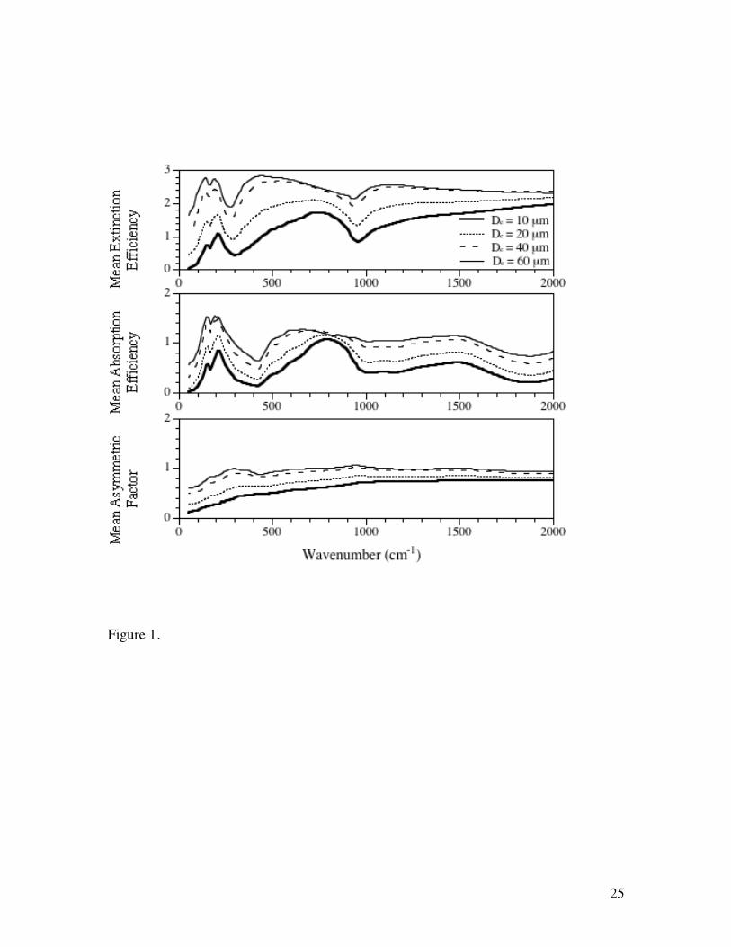
Figure 1 shows the variation of the mean single-scattering properties for four particle

sizes (De = 10, 20, 40 and 60 µm ) as functions of the wavenumber of the incident

radiation. Generally, the scattering properties of small particles are different from those

of large particles because the scattering of radiation by small particles is closer to those

for the regime of Rayleigh scattering [Yang et al., 2003b]. Additionally, the variation of

the averaged absorption efficiency for smaller particle sizes is similar to that of the

imaginary part of ice refractive index [see Warren, 1984].

A line-by-line (LBL) radiative transfer model developed by Heidinger [1998] is used

for calculating the background optical depths of clear-sky atmospheric layers due to the

absorption by various radiatively important gases (e.g. H2O, CO2, O3, N2O, CO, CH4,

etc.) with the line parameters from HITRAN-2000 [Rothman et al., 1998]. The

continuum absorption of water vapor and other gases are considered on the basis of the

approach developed by Tobin et al. [1999]. The broadband outgoing TOA LW and WIN

8

band radiances are calculated for each FOV using the DISORT [Stamnes et al., 1988]

implemented with 32 streams.

Following tradition in the liteature, we specify the optical thickness of a cirrus cloud in

reference to its value at a visible wavelength, that is, the cirrus optical thickness in the

LW spectrum can be specified as follows:

!

" =<Q

e>

2"vis

(8)

where !vis

is the visible optical depth, and we assume that the mean extinction efficiency

of ice particles at a visible wavelength is 2. In Eq. (8),

!

<Qe

> is the mean extinction

efficienciy defined by Eq. (4) for a given infrared wavelength. As the TOA outgoing

radiance depends on the cloud effective particle size, four effective diameters (De = 10,

20, 40 and 60µm ) are specified for the radiative transfer computations. Additionally, five

values of the visible optical depth (!vis

= 0.03, 0.1, 0.15, 0.2, and 0.3) are specified for

each particle size. A library is developed for the outgoing radiances associated with the

values of the visible optical depth !vis

ranging from 0.03 to 0.3 and each effective particle

size.

3. Results

Figure 2 shows the observed and calculated LW and WIN band radiances and also the

corresponding relative differences for each FOV. Both the observed and calculated

radiances are for clear-sky conditions and their relative differences (ε) are defined as

follows:

!

" =(robs# r

cal)

rcal

$100(%) (9)

9

where r is the outgoing either LW or WIN-channel radiance. The subscripts obs and cal

indicate the observed and calculated quantities, respectively. The radiances computed for

cloud-free FOVs are larger than their observed counterparts for both the CERES LW and

WIN channels. We suggest that these differences be explained in large part by the

presence of thin cirrus. An important point to note is that the cloud mask is flagged as

cloudy when the assumed optical thickness of the cloud is larger than approximately 0.2

~ 0.3 and we use only CERES FOVs declared as cloud free in the SSF product; that is,

thin cirrus clouds with optical thickness less than 0.3 might be missed in the cloud

detection.

The relative differences defined in Eq. (9) in the case for the LW radiance are between

-2.1% and -8.3% with a mean value of -4.2%. The CERES FOVs are separated by scene

type into two categories: over ocean and over land [Loeb et al., 2003b]. Large differences

between the measurements and simulations occur for 7 nighttime FOVs whose scene

types are over land. The relative differences are approximately -8.0% for the 4 FOVs

(2004070603 UTC, 36~39th FOV), and -7.0% for the other 3 FOVs (2004072903 UTC,

74~76th FOV). The relative differences in WIN channel radiances are between -1.7 and -

10.6% with a mean value of -4.5%. The WIN channel radiances are calculated in the

spectral range between 8.1 and 11.8 µm [Loeb et al., 2003b].

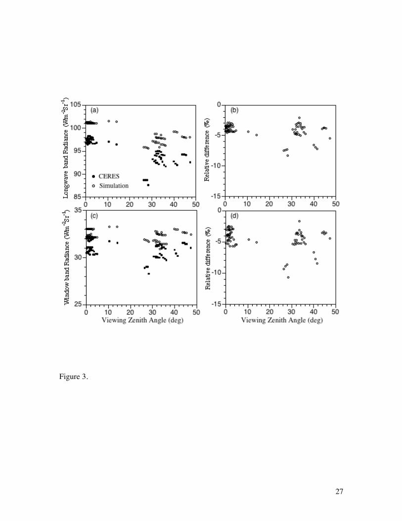
Figure 3 shows both the observed and calculated LW and WIN channel radiances and

their relative differences as functions of the viewing zenith angle. Both the measured and

calculated radiances show the expected limb-darkening features. The angular

distributions of the relative differences are similar for the LW and WIN channels. The

maxima of the relative differences between the theoretical simulations and the

corresponding CERES measurements seem to occur at the viewing zenith angles ranging

from 25° to 30°. Evidently, the observed radiances for the pixels flagged as cloud free are

smaller than the simulated data, and the relative differences can be as large as -8.3% and -

10.6% for the LW and WIN band radiances, respectively, at a viewing zenith angle of

~28°. The outliers in the range between 25° and 30° may not imply something systematic

but need to be further investigated with a larger set of data. These pixels are all over land.

Wilber et al. [1999] adopted scene types from the International Geosphere Biosphere

Programme (IGBP) and developed surface emissivity maps to account for the scene

10

dependence. Surface condition parameters in the CERES SSF products are obtained from

their surface maps. Since a CERES FOV has a 20km spatial resolution at nadir, the

heterogeneity of the surface emissivity over a CERES FOV could cause some errors in

determining the surface parameters.

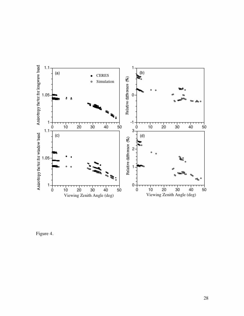
Figure 4 shows both the observed and calculated LW and WIN channel anisotropy

factors and also their relative differences as functions of the viewing zenith angle. The

anisotropy factors for the LW and WIN radiation are calculated from:

!

A(") =#I (")

F, (10)

where θ is the viewing zenith angle, I(θ) and F are radiance and the corresponding flux at

a reference level, respectively. The ADMs are used to obtain the LW and WIN broadband

fluxes from the observed radiances. There are 45 ADMs for clear-sky daytime and

nighttime conditions over various surfaces. As shown in Fig. 4 (the upper left panel for

the LW channel and the lower panel for the WIN channel), the anisotropic factor

decreases as the viewing zenith angle increases.

For the viewing zenith angles between 0° and 50°, the values of the anisotropic factors

for the observed radiances are larger than those calculated except for some pixels for the

viewing zenith angles larger than 27° for the LW bands. The relative differences between

the measurements and simulations become smaller for both the LW and WIN bands as

the viewing zenith angle approaches to 50°. The relative differences of the anisotropy

factor for the LW band are between -0.23% (at θ = 45.5°) and 0.76% (at θ = 0.1°) with a

mean value of 0.19%, and for the WIN band between 0.29% (at θ = 45.5°) and 2.5% (at θ

= 0.1°) with a mean value of 1.26%. The TOA flux for a clear sky might be

underestimated with a larger anisotropy factor. As an example using a typical clear-sky

LW flux of 300 Wm-2, if the CERES anisotropic factor is overestimated by a typical

value of 0.2% because of potential cirrus contamination, the LW flux would be

underestimated by approximately 0.2%, or 0.6 Wm-2, in the regions where these cirrus

clouds are present. Loeb et al. [2003a] showed that the difference between direct

integration and the flux converted from the radiance using the LW ADMs is below 0.5

11

Wm-2. The values of the LW anisotropy factor in the present study show quite small

relative differences, which means that the differences of the anisotropy factor values

between the CERES SSF products and the simulated could be within the uncertainty

range of the ADM models.

Figure 5 (a) shows the inferred optical depth from minimizing the differences between

the observed and calculated LW radiance as a function of the viewing zenith angle. The

inferred optical thickness for each FOV is essentially below 0.3 for each De value. For

more than 70 of the FOVs, the optical thicknesses are below 0.2, which also depend on

De. For the viewing zenith angles between 25° and 30°, the optical thicknesses are larger

than those at other angles. This is not unexpected, given the results of Fig. 3 (i.e. the

difference between the observed and calculated radiance is large). Fig. 5 (b) shows the

inferred cirrus optical thickness obtained by minimizing the differences between the

observed and the calculated WIN channel radiances as a function of the viewing zenith

angle. The optical thickness pertaining to each FOV tends to be below 0.3 with an

exception of just two FOVs (τvis = 0.31 and 0.34) when De = 10µm . As the effective

diameter increases, the values of the optical thickness converge for both the LW and

WIN channels. This feature is associated with the variation of the averaged single-

scattering properties of droxtals shown in Fig. 1.

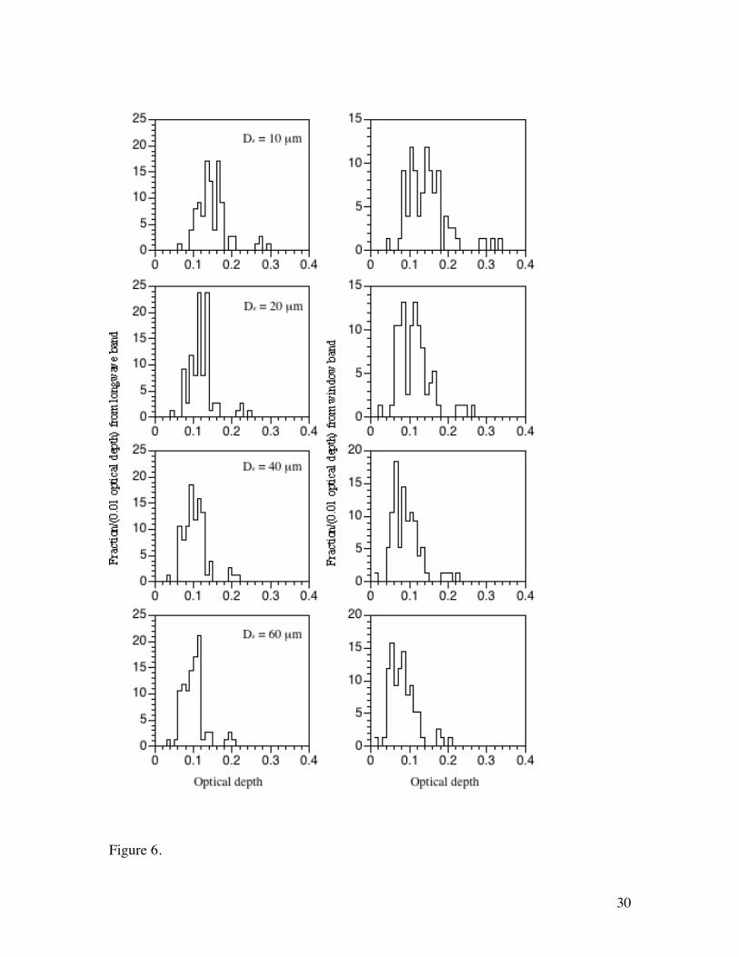
In Fig. 6, the left panels show the histograms of cirrus optical thicknesses inferred

from the differences between the observed and calculated LW radiances. As the effective

diameter increases, the distribution of the optical thickness is shifted towards smaller

values (see Table 1) and the distribution narrows. The optical thickness distribution is

similar to that of Dessler and Yang [2003; see their Fig. 3] for the frequent occurrence of

thin cirrus clouds. The right panels in Fig. 6 show the distributions of optical thicknesses

inferred from the differences between the observed and calculated WIN channel

radiances. Similar to the cases pertaining to the left panels in Fig. 6, the distribution of

the optical thickness derived from the WIN band also shifts to smaller values with an

increase of the effective diameter (see Table 1). The peaks of the frequency distributions

of the optical thickness are shifted to slightly smaller values.

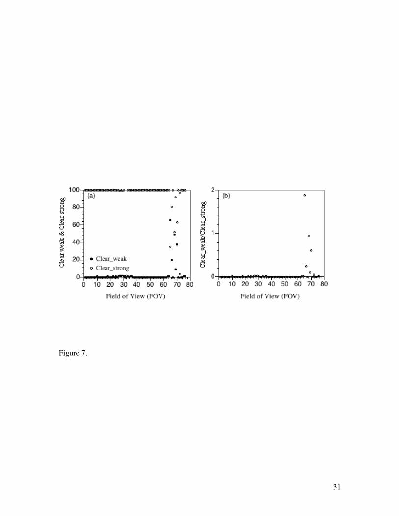
Figure 7 shows clear-strong and clear-weak percent coverage of each CERES FOV. In

the CERES cloud mask, there are several clear subcategories such as clear-strong and

12

clear-weak. The CERES SSF products provide cloud mask information on clear-strong

(or, weak) percent coverage. Note that, for the CERES data, the clear-strong (or, weak)

percent coverage is a weighted percentage of clear-strong (or, weak) MODIS pixels

within the CERES FOV. For the data set used in this study, 70 FOVs out of the 76 FOVs

have over 90% clear-strong coverage and 66 FOVs have 100% clear-strong coverage.

The ratio of clear-weak percent coverage to clear-strong percent coverage is almost zero

except for a few FOVs.

4. Sensitivity Study

The radiative transfer simulations require knowledge of the surface temperature and

emissivity, and the vertical atmospheric temperature and water vapor profiles. We

performed various sensitivity studies for clear-sky conditions with a ±1 K bias of the

surface temperature, a ±2% bias of the surface emissivity, a ±1 K bias of the vertical

sounding temperature, and a ±5% bias of water vapor in the lower atmospheric layers in

conjunction with a ±50% bias of water vapor in the upper atmospheric layers.

Figures 8-11 show both the observed and calculated radiances as well as their relative

differences for both the LW and WIN bands. The radiances are calculated with a ±2%

bias of the surface emissivity (Fig. 8). Although a ±2% bias of the surface emissivity is

considered, the calculated LW and WIN channel radiances are larger than their observed

counterparts. The average relative differences of the observed and calculated LW (WIN)

channel radiance are -3.57% (-3.11%) with a -2% bias of the surface emissivity and -

4.6% (-5.5%) with a +2% bias of the surface emissivity. The CERES instrument accuracy

requirements are 0.6 Wm-2Sr-1 for the LW band and 0.3 Wm-2Sr-1 for the WIN band [Lee

et al., 1997], which are indicated as the error bars in Figs. 8-11.

In Fig. 9 the LW and WIN channel radiances are calculated with a ±1 K bias of the

surface temperature. The average relative difference of the observed and calculated LW

(WIN) channel radiances are –3.62% (-3.22%) with a –1K bias of the surface temperature

and -4.74% (-5.68%) with a +1K bias of the surface temperature. The effects of a +1 K (-

13

1 K) bias in the surface temperature and a +2% (-2%) bias in the surface emissivity are

similar for both the LW and WIN channel radiances.

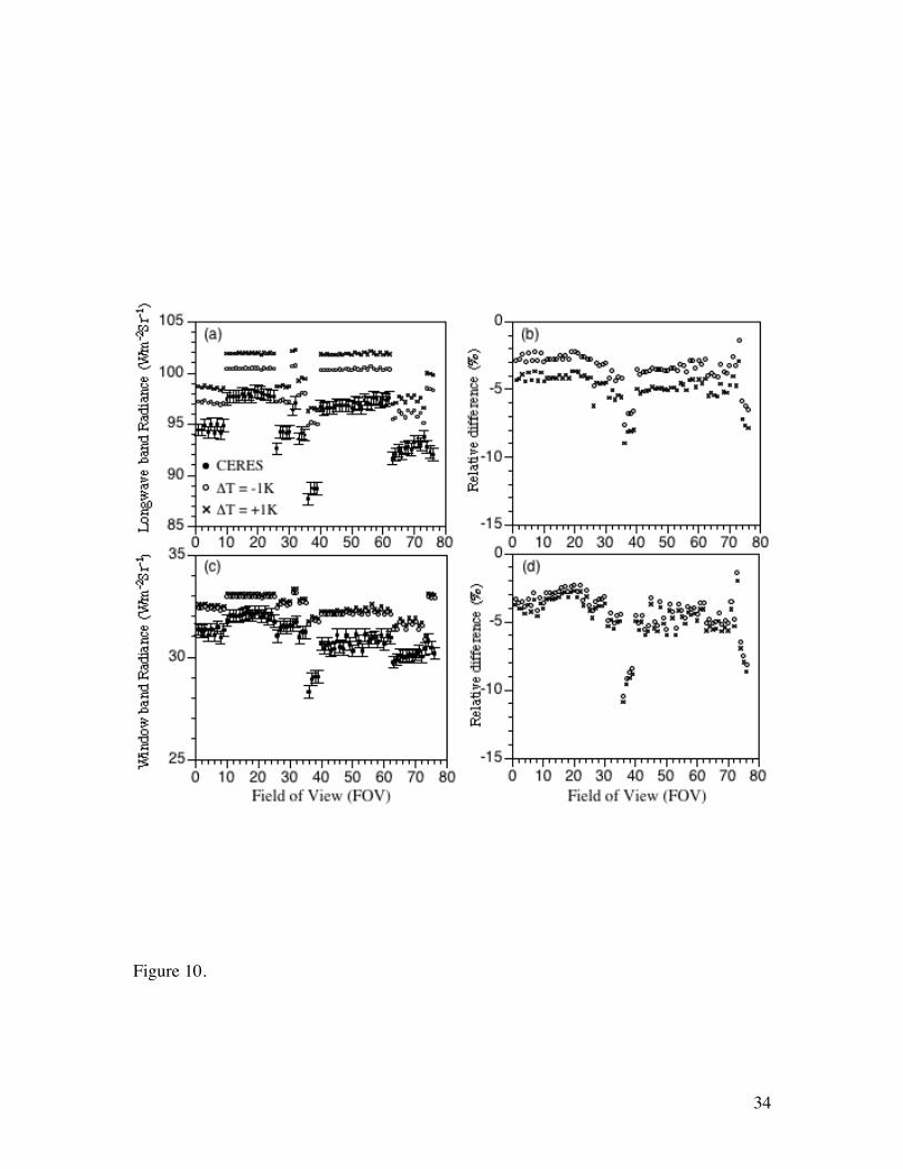
The LW and WIN channel radiances are calculated assuming a ±1 K bias in a given

vertical temperature profile (Fig. 10). The average relative difference in the LW (WIN)

channel radiances between the observed and calculated values is –3.47% (-4.29%) with a

–1K bias of the temperatures and –4.9% (-4.76%) with a +1 K bias of temperatures. A

+1K (-1K) bias of the vertical temperature profile causes the changes in the LW channel

radiances with a similar order to the case for a +2% (-2%) bias of the surface emissivity,

and little influence on the WIN channel radiances.

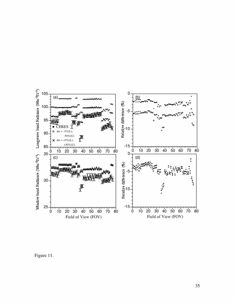
The LW and WIN channel radiances are calculated with a ±5% bias in the water vapor

amount for lower tropospheric layers in conjunction with a ±50% bias in the water vapor

amount for upper tropospheric layers (Fig 11). An upper (lower) tropospheric layer in this

study is defined as one in which the temperature is below (above) 273 K. The average

relative difference of the LW (WIN) channel radiances between the observed and

calculated values is –6.12% (-4.83%) with a negative bias of water vapor and –2.87% (-

4.25%) with a positive bias of water vapor. Both the negative (positive) bias of water

vapor and a +1K (-1K) bias in the vertical temperature profile cause some changes on the

LW channel radiance but have little effects on the WIN channel radiance. Since the

radiance in the window region is less sensitive to water vapor amount, the variability of

the radiance in the LW channel is larger than that in the WIN channel.

5. Discussion and conclusions

We investigate a set of 76 CERES FOVs that are deemed to be free of clouds by the

operational CERES cloud clearing procedure. The clear-sky radiances are calculated

using a forward radiative transfer model and compared to the measured radiances. The

temperature and humidity profiles are taken from the rawinsondes launched during the

CRYSTAL-FACE campaign in July 2002. We find that the calculated LW and WIN

channel radiances are larger than those measured by CERES. A possible mechanism for

these differences could be the presence of thin cirrus clouds. Clouds with optical

14

thicknesses less than approximately 0.2 to 0.3 are difficult to detect and much less

analyze.

In the present analyses of CERES data, the cirrus optical thicknesses range generally

between 0.03< τvis < 0.3. It seems that thin cirrus clouds were ubiquitous in this region

around Florida during CRYSTAL-FACE. The results obtained herein are somewhat

similar to the result by Dessler and Yang [2003] who noticed that about one third of the

MODIS pixels flagged as confidently clear actually contained detectible thin cirrus. As

their study used the MODIS 1.38µm band, their approach is not applicable for analyzing

nighttime data. The present study is focused on a set of 76 CERES FOVs rather than the

large number of daytime MODIS pixels (>107) and wide geographical region (tropical

area) encompassed in their study. We find that as ice cloud effective diameter increases,

the optical thickness inferred from both the LW and WIN channels converges. This study

is complementary to Dessler and Yang [2003], as they used daytime MODIS

observations and most of the CERES FOVs used in this study are for nighttime.

The anisotropic factors show some differences between the observed and calculated

values at the LW and WIN bands. The comparison shows that the difference decreases

with increasing the viewing zenith angle to 50°. Since anisotropy factors of the observed

radiances are larger than those of the calculated radiances for the viewing zenith angles

between 0° and 50°, it is likely possible to underestimate (by a few percent) CERES LW

and WIN fluxes that are associated with the scenes that flagged as cloud free. The

difference in the anisotropic factors is small compared to the corresponding large

difference in radiance between the CERES observations and the theoretical calculations. The error in flux is related to the error in anisotropic factor. If the CERES anisotropic

factor is overestimated by a typical value of 0.2% due to the neglect of the presence of

thin cirrus clouds within the CERES FOVs, the LW flux would be underestimated by

approximately 0.2%, or 0.6 Wm-2, given a typical clear-sky LW flux of 300 W/m2. An

error would arise in the interpretation of the flux since the FOV is classified as clear sky

rather than cloudy.

A sensitivity study showed that even by accounting for the uncertainties caused by

several factors (excluding the presence of cirrus), such as in the temperature and humidity

profiles, there is still some disagreement between the simulated for both the LW and

15

WIN channel radiances under clear-sky conditions and their CERES observed

counterparts.

While Dessler and Yang [2003] showed thin cirrus clouds are ubiquitous using a

daytime data set, thin cirrus clouds could also be common over Florida region at

nighttime. Therefore, the radiances measured for the FOVs that are identified as “clear-

sky” could be contaminated by the existence of thin cirrus clouds with optical thickness

less than 0.3. Further research using active measurements during nighttime conditions

would be quite useful.

Acknowledgements

The authors thank Andrew Dessler for useful comments and suggestions. This research is

supported by the National Science Foundation (NSF) CAREER Award research grant

(ATM-0239605), a research grant from the NASA Radiation Sciences Proram

(NNG04GL24G), and a subcontract from Science Applications International Corporation

(4400053274).

16

References

Ackerman, S. A., K. I. Strabala, W. P. Menzel, R. A. Frey, C. C. Moeller, and L. E.

Gumley (1998), Discriminating clear sky from clouds with MODIS, J. Geophys. Res.,

103, 32141-32157.

Baum, B. A., A. J. Heymsfield, P. Yang, and S. T. Bedka (2005), Bulk scattering models

for the remote sensing of ice clouds. 1: Microphysical data and models. J. Appl.

Meteorol. (in press).

Chepfer, H., G. Brogniez, and Y. Fouquart (1998), Cirrus clouds microphysical

properties deduced from POLDER observations, J. Quant. Spectrosc. Radiat.

Transfer, 60, 375-390.

Chepfer, H., P. Goloub, J. Riedi, J. F. De Hann, J. W. Hovenier, and P. H. Flamant

(2001), Ice crystal shapes in cirrus clouds derived from POLDER/ADEOS-1, J.

Geophys. Res., 106, 7955-7966.

Dessler, A. E., P. Yang (2003), The Distribution of tropical thin cirrus clouds inferred

from Terra MODIS data, J. Clim., 16, 1241-1247.

Foot, J. S. (1988), Some observations of the optical properties of clouds: II. Cirrus,

Quart. J. Roy. Meteor. Soc. 114, 145-164.

Francis, P. N., A. Jones, R. W. Saunders, K. P. Shine, A. Slingo, Z. Sun (1994), An

observational and theoretical study of the radiative properties of cirrus: Some results

from ICE’89, Quart. J. Roy. Meteor. Soc. 120, 809-848.

Fu, Q. (1996), An accurate parameterization of the solar radiative properties of cirrus

clouds for climate models, J. Clim., 9, 2058-2082.

Fu, Q., W. B. Sun and P. Yang (1999), On model of scattering and absorption by cirrus

nonspherical ice particles at thermal infrared wavelength, J. Atmos. Res., 56, 2937-

2947.

Gao, B.-C., P. Yang, W. Han, R.-R. Li, and W. Wiscombe (2002), An algorithm using

visible and 1.38 channels to retrieve cirrus reflectances from aircraft and satellite

data, IEEE Trans. Geosci. Remote Sensing, 40, 1659-1668.

Geier, E. B., R. N. Green, D. P. Kratz, P. Minnis, W. F. Miller, S. K. Nolan, C. B.

Franklin (2003), Clouds and the Earth’s Radiant Energy System (CERES) Data

17

Management System: Single Satellite Footprint TOA/Surface Fluxes and Clouds

(SSF) Collection Document, http://asd-www.larc.nasa.gov/ceres/collect_guide,

243pp.

Hansen, J. E. (1971), Multiple scattering of polarized light in planetary atmospheres. Part

II. Sunlight reflected by terrestrial water clouds, J. Atmos. Sci., 28, 1400-1426.

Hansen, J. E., and L. D. Travis (1974), Light scattering in planetary atmosphere, Space

Sci. Rev., 16, 527-610.

Heidinger, A. (1998), Nadir sounding of clouds and aerosol in the O2 A-band,

Atmos. Sci. Pap. 650, 226 pp., Colo. State Univ., Fort Colins, Colo.

Jensen, E., D. Starr, and O. B. Toon (2004), Mission investigates tropical cirrus clouds,

Eos Trans. AGU, 85(5), 45, 50.

Kahn, B. H., K. N. Liou, S. Y. Lee, E. F. Fishbein, S. Desouza-Machado, A. Eldering, E.

J. Fetzer, S. E. Hannon, L. L. Strow (2005), Nighttime cirrus detection using

atmospheric infrared sounder window channels and total column water vapor, J.

Geophys. Res., 110(D7), 07203, doi: 10.1029/2004JD005430.

King, M. D., W. P. Menzel, Y. J. Kaufman, D. Tanré, B. C. Gao, S. Platnick, S. A.

Ackerman, L. A. Remer, R. Pincus, and P. A. Hubanks (2003), Cloud and Aerosol

Properties, Precipitable Water, and Profiles of Temperature and Humidity from

MODIS, IEEE Trans. Geosci. Remote Sensing, 41, 442-458.

Lee III, R. B., B. R. Barkstrom, G. L. Smith, J. E. Cooper, L. P. Kopia, and R. W.

Lawrence (1996), The Clouds and the Earth’s Radiant Energy System (CERES)

sensors and preflight calibration plans, J. Atmos. Oceanic Tech., 13, 300-313.

Lee, R. B., B. R. Barkstrom, D. A. Crommclynck,G. L. Smith, W. C. Bolden, J. Paden,

D. K. Pandey, S. Thomas, L. Thornhill, R. S. Wilson, K. A. Bush, P. C. Hess, and W.

L. Weaver (1997), Clouds and the Earth’s Radiant Energy System (CERES)

Algorithm Theoretical Basis Document: Instrument Geolocate and Calibrate Earch

Radiances (Subsystem 1.0), http://asd-www.larc.nasa.gov/ATBD/ATBD.html, 84 pp.

Loeb, N. G., S. Kato, K. Loukachine, and N. M. Smith (2005), Angular distribution

models for top-of-atmosphere radiative flux estimation from the Clouds and the

Earth’s Radiant Energy System instrument on the Terra Satellite, 1, Methodology, J.

Atmos. Oceanic Tech., 22, 338-351.

18

Loeb N. G., K. Loukachine, N. Manalo-Smith, B. A. Wielicki, and D. F. Young (2003a),

Angular Distribution Models for Top-of-Atmosphere Radiative Flux Estimation from

the Clouds and the Earth’s Radiant Energy System Instrument on the Tropical

Rainfall Measuring Mission Satellite. Part II: Validation. J. Appl. Meteor., 42, 1748-

1769.

Loeb, N. G., K. J. Priestley, D. P. kratz, E. B. Geier, R. N. Green, B. A. Wielicki, P. O.

Hinton, and S. K. Nolan (2001), Determination of unfiltered radiances from the

clouds and the earth’s radiant energy system instrument, J. Appl. Meteorol., 40, 822-

835.

Loeb, N. G., N. M. Smith, S. Kato, W. F. Millfer, S. K. Gupta, P. Minnis, and B. A.

Wielicki (2003b), Angular distribution models for top-of-atmosphere radiative flux

estimation from the Clouds and the Earth’s Radiant Energy System Instrument on the

Tropical Rainfall Measuing Mission Satellite, 1, Methodology, J. Appl. Meteorol., 42,

240-265.

Mather, J. H., T. P. Ackerman, M. P. Jensen, and W. E. Clements (1998), Characteristics

of the atmospheric state and the surface radiation budget at the tropical western

Pacific ARM site. Geophys. Res. Lett., 25, 4513-4516.

McFarquhar, G. M., A. J. Heymsfield, J. Spinhirne, and B. Hart (2000), Thin and

subvisual tropopause tropical cirrus: observations and radiative impacts, J. Atmos.

Sci., 57, 1841-1853.

Meyer, K., P. Yang, and B.-C. Gao (2004), Optical thickness of tropical cirrus clouds

derived from the MODIS 0.66- and 1.375 channels, IEEE. Trans. Geosci. Remote

Sensing, 42, 833-841.

Minnis, P., D. F. Young, D. P. Kratz, J. A. Coakley, Jr., M. D. King, D. P. Garber, P. W.

Heck, S. Mayor, and R. F. Arduini (1997), Clouds and the Earth’s Radiant Energy

System (CERES) Algorithm Theoretical Basis Document: Cloud Optical Property

Retrieval (Subsystem 4.3), http://asd-www.larc.nasa.gov/ATBD/ATBD.html, 60 pp.

Minnis, P., D. F. Young, S. Sun-Mack, P. W. Heck, D. R. Doelling, and Q. Trepte

(2003), CERES Cloud Property Retrievals from Imagers on TRMM, Terra, and Aqua,

Proc. SPIE 10th International Symposium on Remote Sensing: Conference on

19

Remote Sensing of Clouds and the Atmosphere VII, Barcelona, Spain, 8-12

September, 37-48.

Mitchell, D. L. (2002), Effective diameter in radiation transfer: General definition,

applications, and limitations, J. atmos. Sci, 59, 2330-2346.

Platnick, S., M. D. King, S. A. Ackerman, W. P. Menzel, B. A. Baum, J. C. Riédi, and R.

A. Frey (2003), The MODIS Cloud Products: Algorithms and Examples from Terra,

IEEE Trans. Geosci. Remote Sensing, 41, 459-473.

Prabhakara, C., D. P. Kratz, J. M. Yoo, G. Dalu, and A. Vernekar (1993), Optically thin

cirrus clouds: radiative impact on the warm pool, J. Quant. Spectrosc. Radiat.

Transfer, 49, 467-483.

Roskovensky, J. K., and K. N. Liou (2003), Detection of thin cirrus from 1.38µm /

0.65µm reflectance ratio combined with 8.6-11µm brightness temperature

difference, Geophys. Res. Lett., 30(19), 1985, doi:10.1029/2003GL018135.

Rossow, W. B. and R. A. Schiffer (1991), ISCCP cloud data products, Bull. Am.

Meteorol. Soc., 72, 2-20.

Rothman, L. S., C. P. Rinsland, A. Goldman, S. T. Massie, D. P. Edwards, J. -M. Flaud,

A. Perrin, C. Camy-Peyret, V. Dana, J. -Y. Mandin, J. Schroeder, A. McCann, R. R.

Gamache, R. B. Wattson, K. Yoshino, K. V. Chance, K. W. Jucks, L. R. Brown, V.

Nemtchinov, and P. Varanasi (1998), The HITRAN Molecular Spectroscopic

Database and HAWKS (HITRAN Atmospheric Workstation): 1997 edition, J. Quant.

Spectrosc. Radiat. Transfer, 60, 665-710.

Sassen, K., M. K. Griffin, and G. C. Dodd (1989), Optical scattering and microphysical

properties of subvisual cirrus clouds and climatic implications, J. Appl. Meteorol., 28,

91-98.Smith, G. L., N. Manalo-Smith, L. M. Avis (1994), Limb-darkening models

from along-track operation of the ERBE scanning radiometer, J. Appl. Meteorol., 33,

74-84.

Smith, G. L., B. A. Wielicki, B. R. Barkstrom, R. B. Lee, K. J. Priestly, T. P. Charlock, P.

Minnis, D. P. Kratz, N. Loeb, and D. F. Young (2004), Clouds and earth radiant

system: an overview, Adv. Space Res., 33, 1125-1131.

20

Stamnes, K., S. C. Tsay, W. Wiscombe, and K. Jayaweera (1988), A numerically stable

algorithm for discrete-ordinate-method radiative transfer in multiple scattering and

emitting layered media, Appl. Opt., 27, 2502-2509.

Tobin, D. C., F. A. Best, P. D. Brown, S. A. Clough, R. G. Dedecker, R. G. Ellingson, R.

K. Garcia, H. B. Howell, R. O. Knuteson, E. J. Mlawer, H. E. Revercomb, J. F. Short,

P. F. W. van Delst, and V. P. Walden (1999), Downwelling spectral radiance

observations at the SHEBA ice station: water vapor continuum measurements from

17 to 26 µm, J. Geophys. Res., 104, 2081-2092.

Trepte, Q., Y. Chen, S. Sun-Mack, P. Minnis, D. F. Young, B. A. Baum, and P. W. Heck

(1999), Scene identification for the CERES cloud analysis subsystem, Proc. AMS 10th

Conf. Atmos. Rad., Madison, WI, 28 June - 2 July, 169-172.

Wang, P.-H., M.P. McCormick, L. R. Poole, W. P. Chu, G. K. Yue, G. S. Kent, and K.

M. Skeens (1994), Tropical high cloud characteristics derived from SAGE II

extinction measurements, Atmos. Res., 34, 53-83.

Wang, P.-H., P. Minnis, M. P. McCormick, G.S. Kent and K. M. skeens (1996), A 6-year

climatology of cloud occurrence frequency from Stratospheric Aerosol and gas

Experiment II observations (1985-1990), J. Geophys. Res., 101, 29407-29429.

Warren, S. G. (1984), Optical constants of ice from the ultraviolet to the microwave,

Appl. Opt., 23, 1206-1225.

Wielicki, B. A., B. R. Barkstrom, E. F. Harrison, R. B. Lee III, G. L. Smith, and J. E.

Cooper (1996), Clouds and the earth’s radiant energy system (CERES): An earth

observing system experiment, Bull. Am. Meteorol. Soc., 77, 853-868.

Wilber, A. C., D. P. Kratz, and S. K. Gupta (1999), Surface emissivity maps for use in

satellite retrievals of longwave radiation, NASA/TP-1999-209362, NASA,

Washington, DC, 35 pp.

Winker, D. M., and C. R. Trepte (1998), Laminar cirrus observed near the tropical

tropopause by LITE, Geophys. Res. Lett., 25, 3351-3354.

Yang, P., B. A. Baum, A. J. Heymsfield, Y. X. Hu, H.-L. Huang, S.-C. Tsay, S.

Ackerman (2003a), Single-Scattering properties of droxtals, J. Quant. Spectrosc.

Radiat. Transfer, 79-80, 1159-1169.

21

Yang, P., M. G. Mlynczak, H, Wei, D. P. Kratz, B. A. Baum, Y. X. Hu, W. J. Wiscombe,

A. Heidinger, and M. I. Mishchenko (2003b), Spectral signature of ice clouds in the

far-infrared region: Single-scattering calculations and radiative sensitivity study, J.

Geophys. Res., 108(D108), 4569, doi:10.1029/2002JD003291.

Yang, P., H. Wei, H.-L. Huang, B. A. Baum, Y. X. Hu, G. W. Kattawar, M. I.

Mishchenko, and Q. Fu (2005), Scattering and absorption properties of various

nonspherical ice particles in the infrared and far-infrared spectral region, Appl. Opt.,

44, 5512-5523.

Zhang, Z. B., P. Yang, G. W. Kattawar, S.-C. Tsay, B. A. Baum, Y. X. Hu, A. J.

Heymsfield, and J. Reichardt (2004), Geometric Optics Solution to light scattering by

droxtal ice crystals, Appl. Opt., 43, 2490-2499.

22

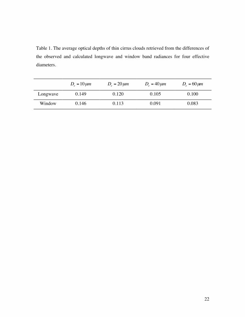
Table 1. The average optical depths of thin cirrus clouds retrieved from the differences of

the observed and calculated longwave and window band radiances for four effective

diameters.

De=10µm D

e= 20µm D

e= 40µm D

e= 60µm

Longwave 0.149 0.120 0.105 0.100

Window 0.146 0.113 0.091 0.083

23

Figure 1. Averaged extinction efficiency, absorption efficiency and asymmetry factor for

droxtal ice crystals with sizes of 10, 20, 40, and 60 µm in the spectral region from 50 to

2000 cm-1.

Figure 2. (a) The observed and calculated TOA outgoing longwave band radiances, (b)

the relative differences for the computed and observed outgoing longwave band

radiances, (c) the window band radiance, (d) relative differences for the computed and

observed outgoing window band radiances. CERES FOVs flagged as cloud free have

been chosen, which are located within 0.25 degree in both latitude and longitude over 4

atmospheric sounding locations during CRYSTAL-FACE period (July 2002).

Figure 3. Similar to Fig. 2, except that the x-axis is for the viewing zenith angle in Fig. 3.

Figure 4. Anisotropy factors provided by the CERES SSF products in comparison with

the present simulations. Panel (a) is for the longwave band and panel (b) is for the

window band.

Figure 5. Optical depths of thin cirrus retrieved from the difference of the observed

radiances and the simulated counterparts by assuming various effective particle sizes.

Panel (a): retrieval from use of the longwave band data; panel (b) retrieval from use of

the window band.

Figure 6. Distributions of the optical depths of thin cirrus clouds retrieved from the

differences of the observed and simulated radiances by assuming various effective

particle sizes. Left panels are based on the longwave band data; right panels are based on

the window band data.

Figure 7. (a) Clear-srong coverage percent and clear-weak coverage percent and (b) the

ratio clear-weak coverage to clear-strong coverage.

24

Figure 8. (a) The observed and calculated TOA outgoing longwave band radiances, (b)

the relative differences for the computed and observed outgoing longwave band

radiances, (c) the window band radiance, (d) relative differences between the computed

and observed outgoing window band radiances. The radiances are calculated with a bias

of ±2% in the surface emissivity. The error bars 0.6 Wm-2Sr-1 for the longwave band

CERES measurement and 0.3 Wm-2Sr-1 for the window band.

Figure 9. Similar to Fig. 8, except that the radiances are calculated with a bias of ±1 K in

the surface temperature.

Figure 10. Similar to Fig. 8, except that the radiances are calculated with a bias of ±1 K

in the vertical atmospheric temperature profile.

Figure 11. Similar to Fig. 8, except that the radiances are calculated with a bias of ±5% in

lower atmospheric water vapor amount in conjunction with a ±50% in upper atmospheric

water vapor amount. Biases of the same sign are considered together. (L) indicates the

lower troposphere and (U) indicates the upper troposphere.

25

Figure 1.

26

Figure 2.

27

Figure 3.

28

Figure 4.

29

Figure 5.

30

Figure 6.

31

Figure 7.

32

Figure 8.

33

Figure 9.

34

Figure 10.

35

Figure 11.