1

Potential Net Present Value for a Cargo Airline Investment inADS-B Avionics Equipment: A Preliminary Analysis

Dr. George L Donohue (gdonohue@gmu.edu), Ms. Motoko Shimizu, Mr. William Laska and Mr. Ash Shah

Department of Systems Engineering and Operations ResearchSchool of Information Technology and Engineering

ANDThe Institute for Public Policy

October 24, 2001

GEORGE MASON UNIVERSITYFairfax, Virginia 22030-4444

2

TABLE OF CONTENTS

List of Tables 3

List of Figures 3

Executive Summary 4

Background 5

Approach 6

Assumptions 7

Concept of Operations 8

Results 8

Discussion 17

References 18

Appendix A: Cost 19

Appendix B: Benefit 20

Appendix C: Cash Flow 22

3

LIST OF TABLES: Page

Table 1. UPS Fleet Payload and Approach Speed. 7

Table 2. FAA Wake Vortex Separation Standards in Nautical Miles. 9

Table 3. Runway Threshold Crossing Times Required to maintain Wake Vortex Separation 9(seconds) T ij.

Table 4. SDF/UPS Aircraft Probability Distribution P ij for Leading Aircraft I and Trailing 9Aircraft j .

Table 5. Measured flight times (ETMS) for UPS Aircraft flying to SDF, with new departure times (Z) and increased loading or sorting time based on a 60-aircraft/hour-arrival rate (WestBank). 13

Table 6. Measured flight times (ETMS) for UPS Aircraft flying to SDF, with new departuretimes (Z) and increased loading or sorting time based on a 60-aircraft/hour-arrival rate (EastBank). 14

Table 7. Benefit-Cost Summary Table 15

Table A-1. Cost specification for Base Case B ($2.5/lb loading benefit, 2yrs equipage, 15%COM) 18

Table B-1. Fuel Benefits ($18/min) 20

Table B-2. Loading Benefits at $2.50 per pound 20

Table B-3. Loading benefits at $4.00 per pound 20

LIST OF FIGURES:

Figure 1. Louisville, Kentucky Typical Daily Airport Arrival Distribution, ETMS data. 10

Figure 2. Aircraft Inter-Arrival Spacing measured at SDF between 23:00 L and 01:50 11 on November 24/25, 1999.

Figure 3. Histogram of Aircraft Inter-Arrival data showing estimate of the Probability 11 Density Function versus the desired Wake-Vortex separation time.

Figure 4. Arrival / Departure Curve Estimates for SDF showing Increased Capacity potentially available with the Increased Surveillance Accuracy and Situational Awareness provided by ADS-B. 12

Figure 5. Annual Cash Flows 16

Figure 6. NPV 16

Figure 7. Tornado Chart of differences in NPV (at Year 10) 16

4

EXECUTIVE SUMMARY

It has been recognized for several years that the advent of ubiquitous Global PositioningSatellite (GPS) coverage will allow very accurate navigation service and combined with adigital data link, surveillance coverage. The level of surveillance service being providedby the new avionics is better than 10 times more accurate than today’s terminalsurveillance service and has a higher overall availability and reliability than today’ssystem due to the increased level of independent system redundancy.

This analysis is aimed at determining how improved surveillance and situationalawareness can benefit air cargo airport capacity and operational performance. SinceFAA mandated equipage of aircraft with GPS based ADS-B (i.e. position measurementand data link transponders) is not currently envisioned, air cargo operators mustunderstand what the Return On Investment (ROI) will be for equipping their fleet withthis new avionics capability. Two financial parameters are of interest to most air cargoChief Financial Officers (CFOs): the Net Present Value (NPV) of the investment and thetime that it takes to obtain a positive ROI or Break Even Time (BET).

This analysis indicates that the primary benefit provided by the addition of ADS-B tocargo aircraft is the increase in schedule flexibility at both the cargo pick-up city and atthe cargo sorting hub operation. Each cargo airline operator will use this time flexibilityin different ways. The trade-off between increased cargo-loading time and increasedcargo-sorting time is an interesting operations research problem in itself.

The cargo value of time is an important parameter that has not received much attention inairline ROI analysis. It is routine to include passenger value of time in all FAAcost/benefit analysis1. Economic theory dictates that the value of time must be includedin any transportation investment analysis. While fuel direct operating costs (FDOC) canbe calculated with reasonable precision, it is estimated that decreased FDOC2, by itself,does not warrant an investment in ADS-B equipment. Using an estimated UPS cargovalue of time of approximately $200/loading minute with an unusable loading time dead-band of 10 minutes, we estimate that the 10 year Net Present Value for investing in ADS-B avionics would be $420 to $520 million (the Base Case) with a 2 year positive ROI. Itis observed that it is more profitable to take aircraft out of service to equip than to spreadthe equipage over a 5 year D check maintenance cycle. There are a number ofuncertainties in this analysis, and the estimated 10-year NPV ranged between $906million and -$118 million.

Although this study concentrates on the operation of United Parcel Service (UPS) atLouisville (SDF) airport, it is believed that the analysis should be equally valid for mostair cargo airlines. UPS and SDF were chosen for detailed study due to their cooperationin the provision of data and access to their operational details.

1 A typical passenger value of time is approximately $50/flight minute for a 100 passenger airplane.2 Currently estimated to be $18/flight minute for 1999 with a fleet mixture similar to UPS.

5

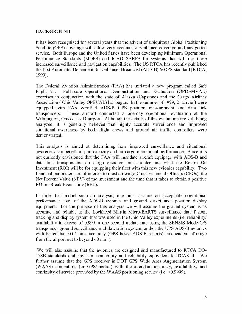
BACKGROUND

It has been recognized for several years that the advent of ubiquitous Global PositioningSatellite (GPS) coverage will allow very accurate surveillance coverage and navigationservice. Both Europe and the United States have been developing Minimum OperationalPerformance Standards (MOPS) and ICAO SARPS for systems that will use theseincreased surveillance and navigation capabilities. The US RTCA has recently publishedthe first Automatic Dependent Surveillance- Broadcast (ADS-B) MOPS standard [RTCA,1999].

The Federal Aviation Administration (FAA) has initiated a new program called SafeFlight 21. Full-scale Operational Demonstration and Evaluation (OPDEMVAL)exercises in conjunction with the state of Alaska (Capstone) and the Cargo AirlinesAssociation ( Ohio Valley OPEVAL) has begun. In the summer of 1999, 21 aircraft wereequipped with FAA certified ADS-B GPS position measurement and data linktransponders. These aircraft conducted a one-day operational evaluation at theWilmington, Ohio class D airport. Although the details of this evaluation are still beinganalyzed, it is generally believed that highly accurate surveillance and improvedsituational awareness by both flight crews and ground air traffic controllers weredemonstrated.

This analysis is aimed at determining how improved surveillance and situationalawareness can benefit airport capacity and air cargo operational performance. Since it isnot currently envisioned that the FAA will mandate aircraft equipage with ADS-B anddata link transponders, air cargo operators must understand what the Return OnInvestment (ROI) will be for equipping their fleet with this new avionics capability. Twofinancial parameters are of interest to most air cargo Chief Financial Officers (CFOs), theNet Present Value (NPV) of the investment and the time that it takes to obtain a positiveROI or Break Even Time (BET).

In order to conduct such an analysis, one must assume an acceptable operationalperformance level of the ADS-B avionics and ground surveillance position displayequipment. For the purpose of this analysis we will assume the ground system is asaccurate and reliable as the Lockheed Martin Micro-EARTS surveillance data fusion,tracking and display system that was used in the Ohio Valley experiments (i.e. reliability/availability in excess of 0.999, a one second update rate using the SENSIS Mode-C/Stransponder ground surveillance multilateration system, and/or the UPS ADS-B avionicswith better than 0.05 nmi. accuracy (GPS based ADS-B reports) independent of rangefrom the airport out to beyond 60 nmi.).

We will also assume that the avionics are designed and manufactured to RTCA DO-178B standards and have an availability and reliability equivalent to TCAS II. Wefurther assume that the GPS receiver is DOT GPS Wide Area Augmentation System(WAAS) compatible (or GPS/Inertial) with the attendant accuracy, availability, andcontinuity of service provided by the WAAS positioning service (i.e. >0.9999).

6

The level of surveillance service being provided by the new avionics is better than 10times more accurate than today’s terminal surveillance service and has a higher overallavailability and reliability than today’s system due to the increased level of independentsystem redundancy. Today’s service is limited by the terminal secondary surveillanceradar (SSR) monopulse beam-width ( ASR-9 has a 1.4 degree beam width) and 4.7second scan rate. It is the slow scan rate, controller-in-the-loop delay time, and lack ofaircraft state vector data that limits the accuracy in the terminal area. This inaccuracylimits aircraft spacing in the terminal area to greater than 4 nmi separation in order toavoid inadvertent violation of aircraft wake vortex separation standards. This limitationwill be discussed more in the results portion of this study as we analyzed baseline data ofthe Louisville (SDF) airport.

Although this study concentrates on the operation of the United Parcel Service (UPS) atSDF, it is believed that the analysis should be equally valid for most air cargo airlines.The details of the NPV analysis will vary based upon each air cargo airline’s investmentand operational strategy. UPS and SDF were chosen for detailed study due to theircooperation in the provision of data and access to their operational details.

APPROACH

In addition to assumptions about surveillance accuracy, reliability, availability andcontinuity of service, one must also make assumptions about avionics cost, installationrates, opportunity cost of investment capital and airline concepts of operation. Air cargoschedules and equipment were obtained from UPS and Enhanced Traffic ManagementSystem (ETMS) data using Dimensions International Flight Explorer Aircraft SituationDisplay software. In order to deal with both proprietary and uncertain data, we haveconducted a parametric analysis (9 combinations of parameters, Cases A – I), varying allof the principle parameters over a representative range. It is hoped that this will producea result that is robust to any as-installed/operational eventuality.

It should be noted that this analysis assumes the FAA controlled ATC system accepts thenew technical performance capability and works harmoniously with the cargo airlines inthe new concept of operations. If the FAA does not allow the cargo airlines to utilizetheir investments in new technology, no benefits will be accrued. This has been observedin the pacific oceanic airspace with the Boeing Future Air Navigation System (FANS)avionics. This is an extremely pertinent example, since both the oceanic and nightairspace are sparsely occupied; yet large aircraft separations are routinely maintained.Aircraft separation is the principal determinant of air transportation capacity. In orderto increase capacity, decrease operational delays and improve air cargo economicperformance, new technologies and separation concepts of operation must be introduced.

7

ASSUMPTIONS

In order to conduct this analysis the following assumptions were made:1. ADS-B purchase cost: $100,0002. ADS-B installation cost: $50,0003. Aircraft out of service opportunity cost (wt avg. per day): $10,300/day/ac4. Aircraft out of service for 5 days for installation5. Avionics annual maintenance cost: $1,0006. Cost of money to purchase and install the avionics: 9% and 15%7. Equipment economic analysis period, straight line cost amortization:10 yr.8. Number of aircraft to be equipped: 2299. Airport where reduced spacing benefits would be accrued: SDF10. Increased revenue from additional loading time at satellite cities: 5,000 lb/hr at $4/lb,

and $2.50/lb.11. Fuel cost savings from reduced time in flight do to direct routing and reduced holding

time benefit: $18/min + / - $6/min.12. Current Aircraft Flight time: UPS schedule and ETMS data taken on 4/16/99, 9/25/99

and 11/24/9913. Optimal Flight Time and fuel burn rate: Jeppesen FliteStar/FliteMap 8.0114. Current SDF aircraft arrival separation: measured 11/24/99 (Figures 2 and 3)15. Aircraft separation at SDF with ADS-B: 2 minutes/runway or 60 ac/hr and 48 ac/hr.16. UPS Fleet Mix: Table 1.

Table 1. UPS Fleet Payload and Approach Speed

AIRCRAFT(Wt. Class/Approach Spd.) NUMBER % OF FLEET Pkg./AC

B757 –200 (H/135 kts) 75 33 7,200B727-100/200 (L/110 kts) 59 26 4,000/5,200DC8-71/73 (H/135 kts) 49 21 9,600B767-300 (H/135 kts) 30 13 12,400B747-100/200 (H/135 kts) 16 07 15,200TOTAL 229 100

Weight Class:H = 255,000 pounds or moreL = 41,000 – 255,000 poundsS = Less than 41,000 pounds

Three different schedule compaction schemes are envisioned: 1) INCREASED SORT -compact all arrivals beginning at 23:00 Local time with 1 minute airport arrival rate (i.e.2 minutes between aircraft per runway); 2) INCREASED LOAD - compact all arrivalsending at 02:00 Local with 1 minute airport arrival rate; and 3) MIXED STRATEGY 2BANK – compact the eastern US bank with arrivals beginning at 00:00 L and compact allwest coast bank aircraft with arrivals ending at 02:00 L. Schedule compaction scheme 3most closely matches today’s operations, dividing the benefits between increased loadrevenue and decreased sorting opportunity costs.

8

CONCEPT OF OPERATIONS

It is hypothesized that the improved surveillance accuracy and pilot/controller situationalawareness will allow aircraft in the low-density, night Enroute and Terminal airspace tomaintain optimum aircraft separation distances. It is assumed that there will be nochange in current FAA separation standards for this analysis. This capability shouldallow the air cargo carrier to maximize the arrival rate at the hub airport. Furthermore,this capability will allow the use of Visual Flight Rules (VFR) procedures and straight inconstant decent approach procedures for night, Marginal VFR (MVFR) and InstrumentFlight Rules (IFR1/2) weather conditions, thus greatly improving schedule predictabilityand reliability.

Delaying satellite airport departure time not only increases cargo load time but alsoallows the aircraft to depart at a less congested time therefore allowing for a morepredictable departure schedule. We assume that wake vortex separation restrictions willbe maintained under all weather conditions. This concept of operations will allow thecargo air carrier to either gain more time to load cargo at satellite airports or to increasethe amount of sort time at the hub airport. This is estimated to be the primary benefit ofADS-B avionics to the cargo air carrier. The secondary benefit is estimated to be reducedenroute fuel costs.

RESULTS

A key measure of airport efficiency is the probability density function of arriving aircraftinter-aircraft spacing. The optimum time interval for a particular airport and mix ofaircraft types can be determined by estimating the separation time between each aircraftweight category based upon maintaining wake vortex separation and using theappropriate aircraft approach speed. The mix of aircraft weight categories can becombined with the matrix of approach time spacing to compute the average minimumaircraft separation time and, therefore, the maximum arrival rate per independent runway.

The single runway capacity can be calculated using the equations discussed by Rakas, Jand Schonfeld, [1998] and Bianco, et. al. [1999].

CP = 3600 / E [ Tij ] ,

Where CP = arrivals/hour/independent runway, and

E [ Tij ] = ΣΣΣΣ Pij Tij ,

Where E [ Tij ] = the expected value of the average minimum wake vortex aircraftseparation time (seconds) across the runway threshold. P ij is the probability that aircraftweight category i is following weight category j. T ij is the time between aircraftweight category i and weight category j over the runway threshold.

9

Table 2 shows the current FAA wake vortex separation standards. Table 3 shows thetime between aircraft assuming the final approach speed shown in Table 1 and theseparation at runway threshold crossing shown in Table 2. Table 4 shows the aircraftprobability matrix for the observed UPS fleet mix at SDF.

Table 2. FAA Wake vortex Separation Standards in Nautical Miles.

LEAD AIRCRAFT HEAVY B757 LARGE SMALL

TRAILINGAIRCRAFT

HEAVY 4 4 2.5 2.5B757 4 4 2.5 2.5LARGE 5 4 2.5 2.5SMALL 6 5 4 2.5

Table 3. Runway Threshold Crossing Times Required to maintain Wake VortexSeparation (seconds) Tij .

LEAD AIRCRAFT HEAVY B757 LARGE SMALL

TRAILINGAIRCRAFT

HEAVY 107 107 67 67B757 107 107 67 67LARGE 164 131 82 82SMALL 240 200 160 100

Table 4. SDF/UPS Aircraft Probability Distribution Pij for Leading Aircraft i andTrailing Aircraft j

LEAD AIRCRAFT HEAVY B757 LARGE SMALL

TRAILINGAIRCRAFT

HEAVY 0.21 0.08 0.07 0.02B757 0.08 0.25 0.07 0.02LARGE 0.07 0.07 0.03 0.00SMALL 0.02 0.02 0.00 0.00

10

For SDF with the UPS fleet mix, a separation of 110 seconds (1:50 minutes) or a 33aircraft arrivals per hour acceptance rate is projected (E [Tij ]). Since SDF has twoindependent parallel runways, the maximum expected value, maintaining wake vortexseparation, would be 66 arrivals per hour. Interviews with SDF tower personnel indicatethey are trying to maintain wake vortex instrument flight rule separation standards fornight operations.

Figure 1. SDF Typical Daily Airport Arrival Distribution, ETMS data. Time isLocal, EST.

Figure 1 shows the hourly arrival rate for SDF airport on a typical day as reported by theETMS data on September 28/29, 1999 (a typical VMC day). Note that the peak arrivalperiod is centered around midnight for SDF due to the UPS air cargo operations thatoccur between 23:00 (EST) and 04:00 (EST). A similar analysis conducted on April 16,1999 showed the same distribution. The ETMS data has a least count report-ability limitof 1 minute and an unknown accuracy (although it is believed to be accurate to withinseveral minutes). More detailed measurements were made on the night of November23/24 at SDF. The weather was clear and visibility was greater than 10 miles. The activerunways were 17L and 17R. Aircraft threshold crossing times were measured toapproximately +/- 15 seconds for each runway. The resulting 60 arrivals were recordedfor the East Coast bank and are shown in Figures 2 and 3. The vertical line in Figure 3equates to roughly the 1:50 minute desired minimum average separation computed forSDF. Note that the most probable arrival spacing is 2:30 minutes and that the distributionis asymmetric with separations measured out to over 5 minutes. This same type ofbehavior has been measured at DFW [Denery, et. al., 1997] and DCA [Donohue, 1999].

SDF ARRIVAL RATE

0

5

10

15

20

25

30

35

40

12 13 14 15 16 17 18 19 20 21 22 23 24 1 2 3 4 5 6 7 8 9 10 11

TIME (24 HOUR)

AIR

CRAF

T AR

RIV

ALS

/ HO

UR

SDF ARRIVAL RATE 9/28-29/99 N = 260

11

Figure 2. Aircraft Inter-Arrival Spacing measured at SDF between 23:00 (EST) and01:50 (EST) on November 24/25, 1999.

Figure 3. Histogram of Aircraft Inter-Arrival data showing estimate of theProbability Density Function versus the desired Wake-Vortex separation time.

SDF INTERARRIVAL DISTRIBUTIONS

0:00:00

0:01:26

0:02:53

0:04:19

0:05:46

0:07:12

0:08:38

0:10:05

0:11:31

0:12:58

1 3 5 7 9 11 13 15 17 19 21 23 25 27 29 31 33 35 37

ARRIVAL SEQUENCE

TIM

E B

ET

WE

EN

AR

RI

RW 17 L (11/24/99)

RW 17 R (11/24/99)

SDF AIRCRAFT ARRIVAL DISTRIBUTION

0

5

10

15

20

25

0:30 1:00 1:30 2:00 2:30 3:00 3:30 4:00 4:30 5:00

ARRIVAL INTERVAL (Min.)

NU

MB

ER

AIR

CR

AF

T A

RR 4:14Z - 5:53 Z

(11/24/99)

WAKE VORTEXLIMIT

12

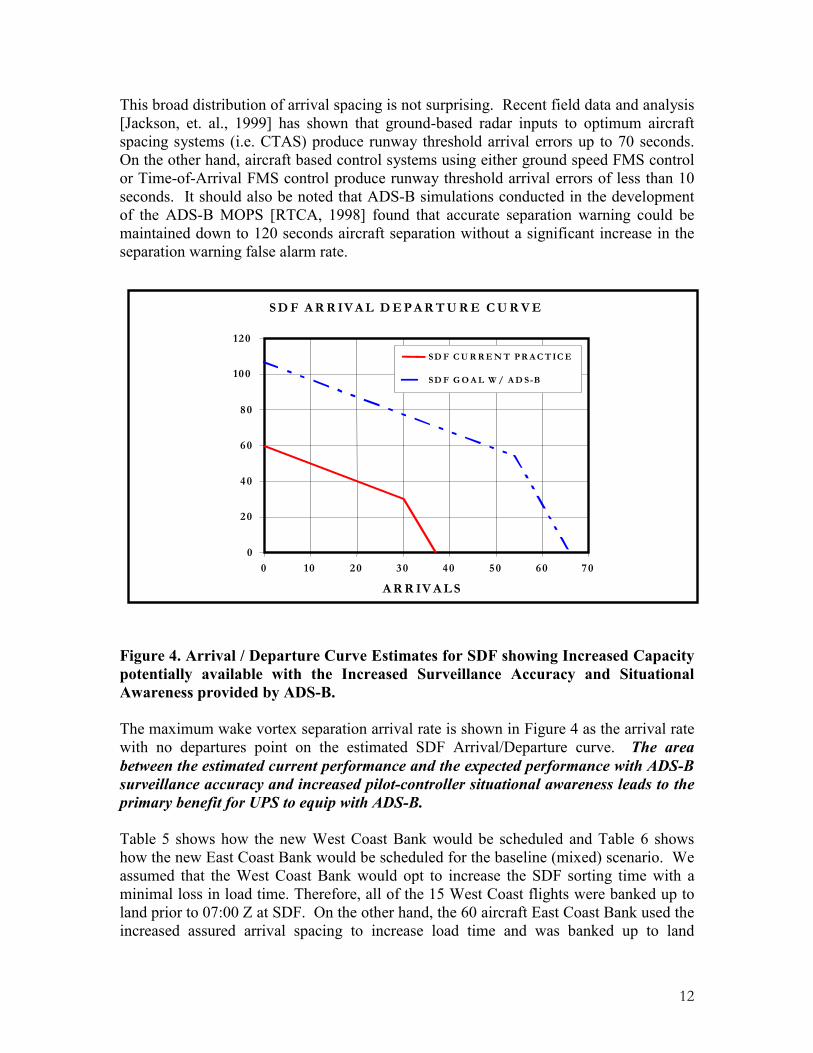
This broad distribution of arrival spacing is not surprising. Recent field data and analysis[Jackson, et. al., 1999] has shown that ground-based radar inputs to optimum aircraftspacing systems (i.e. CTAS) produce runway threshold arrival errors up to 70 seconds.On the other hand, aircraft based control systems using either ground speed FMS controlor Time-of-Arrival FMS control produce runway threshold arrival errors of less than 10seconds. It should also be noted that ADS-B simulations conducted in the developmentof the ADS-B MOPS [RTCA, 1998] found that accurate separation warning could bemaintained down to 120 seconds aircraft separation without a significant increase in theseparation warning false alarm rate.

Figure 4. Arrival / Departure Curve Estimates for SDF showing Increased Capacitypotentially available with the Increased Surveillance Accuracy and SituationalAwareness provided by ADS-B.

The maximum wake vortex separation arrival rate is shown in Figure 4 as the arrival ratewith no departures point on the estimated SDF Arrival/Departure curve. The areabetween the estimated current performance and the expected performance with ADS-Bsurveillance accuracy and increased pilot-controller situational awareness leads to theprimary benefit for UPS to equip with ADS-B.

Table 5 shows how the new West Coast Bank would be scheduled and Table 6 showshow the new East Coast Bank would be scheduled for the baseline (mixed) scenario. Weassumed that the West Coast Bank would opt to increase the SDF sorting time with aminimal loss in load time. Therefore, all of the 15 West Coast flights were banked up toland prior to 07:00 Z at SDF. On the other hand, the 60 aircraft East Coast Bank used theincreased assured arrival spacing to increase load time and was banked up to land

S D F A R R IV A L D E P A R T U R E C U R V E

0

20

40

60

80

100

120

0 10 20 30 40 50 60 70

A R R IV A L S

SD F C U R R E N T P R A C T IC E

SD F G O A L W / A D S-B

13

between 05:00 Z and 06:00 Z at SDF. Pushing the East Coast satellite city departuretimes back has the added advantage of operating in less congested airport and enrouteairspace.

The costs for financing, equipping and operating the UPS fleet are described in AppendixA. Appendix B describes how the benefits are computed. Appendix C looks at ninescenarios (Case A through I) analyzing each relative to fuel and loading benefits, annualcosts, and NPV.

Table 5. West Coast Bank measured flight times (ETMS) for UPS Aircraft flying toSDF, with new departure times (Z) and increased loading or sorting time based on a60 aircraft / hour arrival rate. Red color indicates negative values.

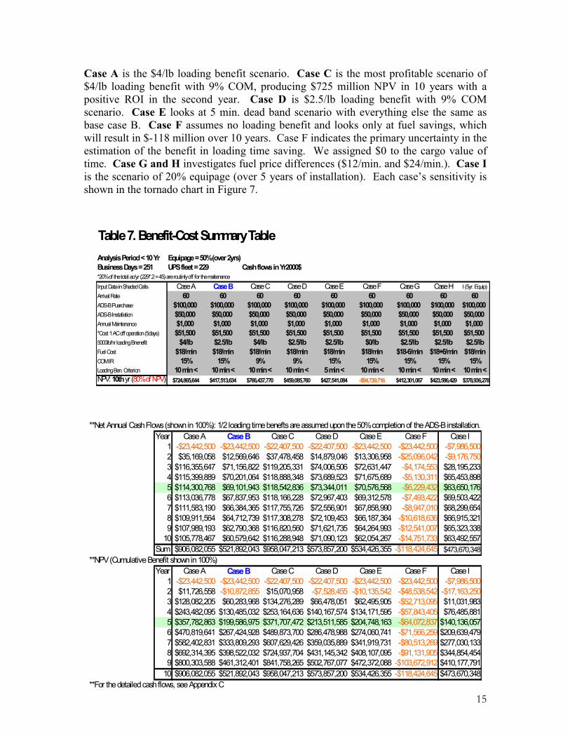
Table 7 and Figures 5, 6 and 7 summarize the costs and benefits of these scenarios. Thebase case, Case B assumes 50% equipage rate (over 2 years of installation), 10 min. deadband, 15% cost of money (COM), $2.5/lb of loading benefit, and $18/min. fuel cost, thatproduces a NPV of $520 million over 10 years with a positive ROI in the second year. Inorder to estimate the effect of not achieving an average of 60 arrivals/hour, we arbitrarilyreduced the computed NPV by 20% in all cases. Therefore the base case NPV will bestated to range from $420 to $520 million.

WEST COAST BANK 9/28 INCREASEDINCREASED DEPTURE NEW ARRIVA9/28/99 ActuFLT TIME SORT LOAD ARR RATE TIME (ZULU)

aircraft origin stinati type dept arr HR:MIN TIME TIME 60/HR (ZULU)SALT LAKE CITY UPS833 SLC SDF B752 3:47 6:29 2:42 0:16 0:16 4:03 6:45ALBUQUERQUE UPS797 ABQ SDF B742 4:18 6:36 2:18 0:10 0:10 4:28 6:46PORTLAND UPS973 PDX SDF DC8Q 3:02 6:42 3:40 0:05 0:05 3:07 6:47SANTA ANA UPS913 SNA SDF B752 3:23 6:49 3:26 0:01 0:01 3:22 6:48DENVER UPS801 DEN SDF B763 4:54 6:52 1:58 0:03 0:03 4:51 6:49LOS ANGELES UPS903 LAX SDF B752 3:31 6:53 3:22 0:03 0:03 3:28 6:50PHONEX UPS857 PHX SDF B763 4:07 6:54 2:47 0:03 0:03 4:04 6:51SACRAMENTO UPS895 MHR SDF B752 3:34 6:55 3:21 0:03 0:03 3:31 6:52SAN DIEGO UPS921 SAN SDF B752 3:29 6:56 3:27 0:03 0:03 3:26 6:53BURBANK UPS907 BUR SDF B752 3:38 7:06 3:28 0:12 0:12 3:26 6:54SAN JOSE UPS941 SJC SDF B752 3:24 7:08 3:44 0:13 0:13 3:11 6:55OAKLAND UPS945 OAK SDF B763 3:34 7:10 3:36 0:14 0:14 3:20 6:56LONG BEACH UPS905 LGB SDF B763 3:47 7:12 3:25 0:15 0:15 3:32 6:57SEATTLE UPS981 BFI SDF B763 3:42 7:18 3:36 0:20 0:20 3:22 6:58ONTARIO UPS917 ONT SDF DC8Q 4:06 7:22 3:16 0:23 0:23 3:43 6:59

TOTAL 2:24 2:24

14

Table 6. East Coast Bank measured flight times (ETMS) for UPS Aircraft flying to SDF, with newdeparture times (Z) and increased loading or sorting time based on a 60 aircraft / hour arrival rate.Red color indicates negative values.

15

Case A is the $4/lb loading benefit scenario. Case C is the most profitable scenario of$4/lb loading benefit with 9% COM, producing $725 million NPV in 10 years with apositive ROI in the second year. Case D is $2.5/lb loading benefit with 9% COMscenario. Case E looks at 5 min. dead band scenario with everything else the same asbase case B. Case F assumes no loading benefit and looks only at fuel savings, whichwill result in $-118 million over 10 years. Case F indicates the primary uncertainty in theestimation of the benefit in loading time saving. We assigned $0 to the cargo value oftime. Case G and H investigates fuel price differences ($12/min. and $24/min.). Case Iis the scenario of 20% equipage (over 5 years of installation). Each case’s sensitivity isshown in the tornado chart in Figure 7.

Table 7. Benefit-Cost Summary TableAnalysis Period < 10 Yr Equipage = 50% (over 2yrs)Business Days = 251 UPS fleet = 229 Cash flows in Yr2000$*20% of the total ac/yr (229*.2 = 45) are routinly off for the maitenance Input Data in Shaded Cells Case A Case B Case C Case D Case E Case F Case G Case H I (5yr. Equip)Arrival Rate 60 60 60 60 60 60 60 60 60ADS-B Puarchase $100,000 $100,000 $100,000 $100,000 $100,000 $100,000 $100,000 $100,000 $100,000ADS-B Installation $50,000 $50,000 $50,000 $50,000 $50,000 $50,000 $50,000 $50,000 $50,000Annual Maintenance $1,000 $1,000 $1,000 $1,000 $1,000 $1,000 $1,000 $1,000 $1,000*Cost 1 AC off operation (5days) $51,500 $51,500 $51,500 $51,500 $51,500 $51,500 $51,500 $51,500 $51,5005000lb/hr loading Bnenefit $4/lb $2.5/lb $4/lb $2.5/lb $2.5/lb $0/lb $2.5/lb $2.5/lb $2.5/lbFuel Cost $18/min $18/min $18/min $18/min $18/min $18/min $18-6/min $18+6/min $18/minCOM IR 15% 15% 9% 9% 15% 15% 15% 15% 15%Loading Ben. Criterion 10 min < 10 min < 10 min < 10 min < 5 min < 10 min < 10 min < 10 min < 10 min <NPV: 10th yr (80% of NPV) $724,865,644 $417,513,634 $766,437,770 $459,085,760 $427,541,084 -$94,739,716 $412,301,067 $423,586,429 $378,936,278

**Net Annual Cash Flows (shown in 100%): 1/2 loading time benefts are assumed upon the 50% completion of the ADS-B installation.Year Case A Case B Case C Case D Case E Case F Case I

1 -$23,442,500 -$23,442,500 -$22,407,500 -$22,407,500 -$23,442,500 -$23,442,500 -$7,986,5002 $35,169,058 $12,569,646 $37,478,458 $14,879,046 $13,306,958 -$25,096,042 -$9,176,7503 $116,355,647 $71,156,822 $119,205,331 $74,006,506 $72,631,447 -$4,174,553 $28,195,2334 $115,399,889 $70,201,064 $118,888,348 $73,689,523 $71,675,689 -$5,130,311 $65,453,8985 $114,300,768 $69,101,943 $118,542,836 $73,344,011 $70,576,568 -$6,229,432 $63,650,1766 $113,036,778 $67,837,953 $118,166,228 $72,967,403 $69,312,578 -$7,493,422 $69,503,4227 $111,583,190 $66,384,365 $117,755,726 $72,556,901 $67,858,990 -$8,947,010 $68,299,6548 $109,911,564 $64,712,739 $117,308,278 $72,109,453 $66,187,364 -$10,618,636 $66,915,3219 $107,989,193 $62,790,368 $116,820,560 $71,621,735 $64,264,993 -$12,541,007 $65,323,338

10 $105,778,467 $60,579,642 $116,288,948 $71,090,123 $62,054,267 -$14,751,733 $63,492,557Sum $906,082,055 $521,892,043 $958,047,213 $573,857,200 $534,426,355 -$118,424,645 $473,670,348

**NPV (Cumulative Benefit shown in 100%)Year Case A Case B Case C Case D Case E Case F Case I

1 -$23,442,500 -$23,442,500 -$22,407,500 -$22,407,500 -$23,442,500 -$23,442,500 -$7,986,5002 $11,726,558 -$10,872,855 $15,070,958 -$7,528,455 -$10,135,542 -$48,538,542 -$17,163,2503 $128,082,205 $60,283,968 $134,276,289 $66,478,051 $62,495,905 -$52,713,095 $11,031,9834 $243,482,095 $130,485,032 $253,164,636 $140,167,574 $134,171,595 -$57,843,405 $76,485,8815 $357,782,863 $199,586,975 $371,707,472 $213,511,585 $204,748,163 -$64,072,837 $140,136,0576 $470,819,641 $267,424,928 $489,873,700 $286,478,988 $274,060,741 -$71,566,259 $209,639,4797 $582,402,831 $333,809,293 $607,629,426 $359,035,889 $341,919,731 -$80,513,269 $277,030,1338 $692,314,395 $398,522,032 $724,937,704 $431,145,342 $408,107,095 -$91,131,905 $344,854,4549 $800,303,588 $461,312,401 $841,758,265 $502,767,077 $472,372,088 -$103,672,912 $410,177,791

10 $906,082,055 $521,892,043 $958,047,213 $573,857,200 $534,426,355 -$118,424,645 $473,670,348**For the detailed cash flows, see Appendix C

0

4

Figure 5. Annual Cash Flows

-$40,000-$20,000

$0$20,000$40,000$60,000$80,000

$100,000$120,000$140,000

1 2 3 4 5 6 7 8 9 10

(in $

1000

)

Year

Ben

efit

Case ACase BCase CCase DCase ECase I

Figure 6. NPV

-$200,000

$0

$200,000

$400,000

$600,000

$800,000

$1,000,000

$1,200,000

1 2 3 4 5 6 7 8 9 10

(in $

1000

)

Year

NPV

Case A

Case B

Case C

Case D

Case E

Case I

Figure 7. Differences in NPV (at the Year 10)

F

H$-.4

$12.5

B $436

-$800 -$600 -$400 -$200Differences in $Millions based on

Differences(NPV)

$52

DC

$-64E

$.G

$-48

I

16

$384

ase Case B = $0

$0 $200 $400 $600

A

the Base Case B (NPB = $522 Million)

17

DISCUSSION:

This analysis indicates that the primary benefit provided by the addition of ADS-B tocargo aircraft is the increase in schedule flexibility at both the cargo pick-up city and atthe cargo sorting hub operation. Each cargo airline operator will use this time flexibilityin different ways. The trade-off between increased cargo-loading time and increasedcargo-sorting time is an interesting operations research problem in itself. The cargo valueof time is an important parameter that has not received much attention in airline ROIanalysis. It is routine to include passenger value of time in all FAA cost/benefit analysis.Economic theory dictates that the value of time must be included in any transportationinvestment analysis. If there was no value of passenger and/or cargo time, there wouldbe no investment in high-speed transportation and we would still be moving betweencities on ox carts.

The estimated 10 year NPV for a UPS investment in ADS-B equipment for its entire fleetranges between $378 million (Case I, 80% of the estimated NPV) and $958 million (CaseC) with a break even time less than 24 months except for cases F and I. The base case(Case B) 10th year NVP is estimated to range between $420 to $520 million. The primaryuncertainty for this estimate is the cargo value of time and the unusable increase indeparture schedule flexibility (or dead band, which ranged between 5 and 10 minutes).The tornado chart in Figure 7 indicates the range of these variations. When the noloading time benefits are assumed (fuel savings only), the 10-year NPV is a - $118million.

While fuel direct operating costs (FDOC) can be calculated with reasonable precision, itis estimated that decreased FDOC, by itself, does not warrant an investment in ADS-Bequipment. During the course of this analysis, an potential new collaborative decisionmaking (CDM) opportunity became apparent, however. Most of the FDOC savings areaccrued by the East Coast bank in getting direct routes to SDF after 11pm. It is not clearhow UPS can ensure that the FAA will give them direct routes even with the extracapacity at SDF that ADS-B equipment should provide.

An entirely ADS-B equipped fleet of aircraft gives the UPS operations center the abilityto have high fidelity surveillance of their aircraft beyond 100 miles (depending on thechoice of data-link, perhaps out to over 200 miles). It is a straightforward step topurchase software (e.g. any ADS-B aircraft tracking software equivalent to the Micro-EARTS system) that will track and display the arriving traffic pattern. Either the NASAdeveloped CTAS TMA algorithms or the FAA/MITRE developed URET algorithms canprovide optimum runway assignment and aircraft separation to maximize enroute to finalapproach traffic management. Even if the FAA cannot provide this capability to SDFbecause of funding limitations, UPS can acquire this system capability in a relativelystraightforward fashion. The UPS operations center is collocated on the SDF airport andcan communicate the arrival sequencing and spacing information directly to the FAATRACON and/or to INDIANAPOLIS, ATLANTA or MEMPHIS Center. It would bedesirable for NEXRAD convective weather to be overlaid on this display, but adding thiscapability may be relatively difficult.

18

ACKNOWLEDGEMENT:

This work was conducted through the financial support of the Federal AviationAdministration (principle author), George Mason University and a grant from UnitedParcel Services Aviation Technology. The opinions expressed in this study are those ofthe authors and do not represent the views of the sponsoring organizations. Any errors oromissions are ours alone.

REFERENCES:

Airline Business,(1999) Top 50 Cargo Airline Rankings – 1998, November, pg.61.

Bianco, L., Dell’Olmo, P. and S. Giordani, (1999) “ Coordination of Traffic Flows in theTMA”, Proceedings of the ATM “99 Workshop on Advanced Technologies and theirImpact on Air Traffic Management in the 21st Century, Capri, Italy, September 26-30.

Denery, Dallas and H. Erzberger, (1997) “The Center-Tracon Automation System:Simulation and Field Testing”, Modeling and Simulation in Air Traffic Management,Bianco, et. al. Editors, Springer Press.

Donohue, G.,(1999) “A Macroscopic Air Transportation Capacity Model: Metrics andDelay Correlation”, Proceedings of the ATM “99 Workshop on Advanced Technologiesand their Impact on Air Traffic Management in the 21st Century, Capri, Italy,September 26-30.

IATA,(1998) Air Cargo Annual: A Statistical Review of the Market in 1997”, October .

Jackson, M., Zhao, Y.J., and R. A. Slattery,(1999) “Sensitivity of Trajectory Prediction inAir Traffic Management”, AIAA Journal of Guidance, Control, and Dynamics, Vol. 22,No. 2, March-April.

Rakas, J. and Schonfeld, P.(1998) “Airspace System Performance after EquipmentOutages”, University of Maryland, Dept. of Civil Engineering TR for FAA Grant 96-G-006.

RTCA,(1998) Minimum Aviation System Performance Standards for AutomaticDependent Surveillance Broadcast (ADS-B), RTCA / DO-242 , February 19.

19

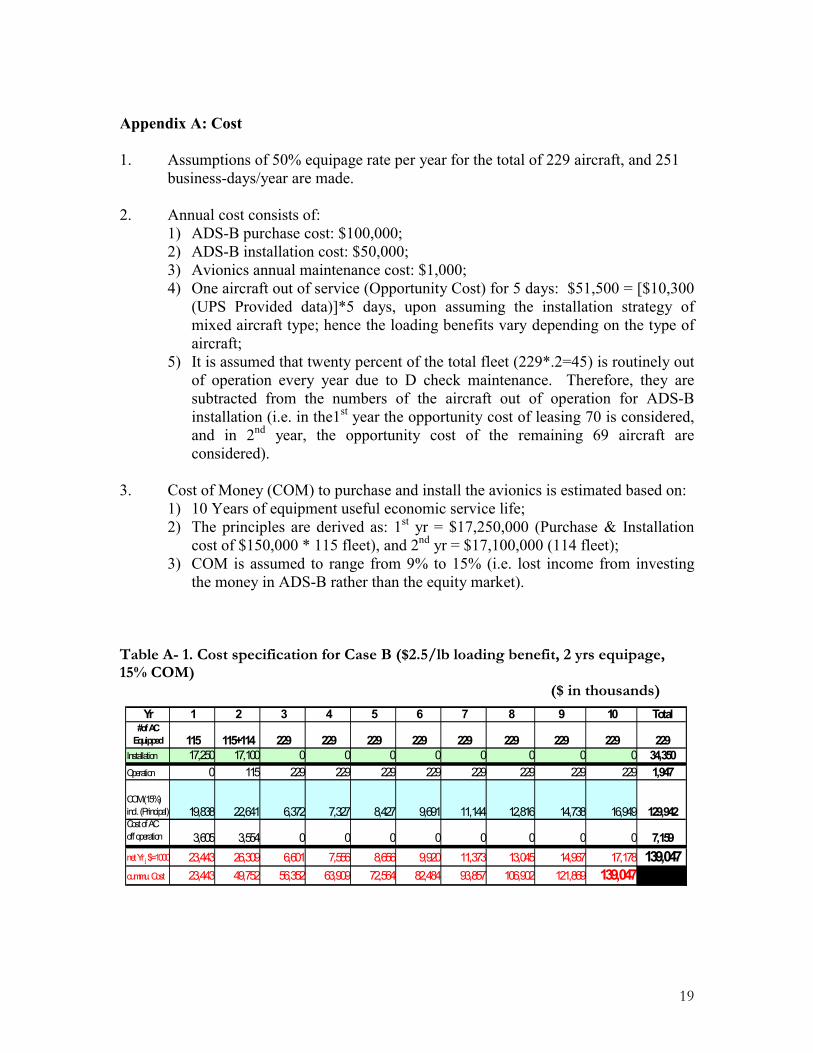
Appendix A: Cost

1. Assumptions of 50% equipage rate per year for the total of 229 aircraft, and 251business-days/year are made.

2. Annual cost consists of:1) ADS-B purchase cost: $100,000;2) ADS-B installation cost: $50,000;3) Avionics annual maintenance cost: $1,000;4) One aircraft out of service (Opportunity Cost) for 5 days: $51,500 = [$10,300

(UPS Provided data)]*5 days, upon assuming the installation strategy ofmixed aircraft type; hence the loading benefits vary depending on the type ofaircraft;

5) It is assumed that twenty percent of the total fleet (229*.2=45) is routinely outof operation every year due to D check maintenance. Therefore, they aresubtracted from the numbers of the aircraft out of operation for ADS-Binstallation (i.e. in the1st year the opportunity cost of leasing 70 is considered,and in 2nd year, the opportunity cost of the remaining 69 aircraft areconsidered).

3. Cost of Money (COM) to purchase and install the avionics is estimated based on:1) 10 Years of equipment useful economic service life;2) The principles are derived as: 1st yr = $17,250,000 (Purchase & Installation

cost of $150,000 * 115 fleet), and 2nd yr = $17,100,000 (114 fleet);3) COM is assumed to range from 9% to 15% (i.e. lost income from investing

the money in ADS-B rather than the equity market).

Table A- 1. Cost specification for Case B ($2.5/lb loading benefit, 2 yrs equipage,15% COM)

($ in thousands)Yr 1 2 3 4 5 6 7 8 9 10 Total

#of AC Equipped 115 115+114 229 229 229 229 229 229 229 229 229

Installation 17,250 17,100 0 0 0 0 0 0 0 0 34,350Operation 0 115 229 229 229 229 229 229 229 229 1,947

COM (15%) incl. (Principal) 19,838 22,641 6,372 7,327 8,427 9,691 11,144 12,816 14,738 16,949 129,942Cost of AC off operation 3,605 3,554 0 0 0 0 0 0 0 0 7,159net Yr j $=1000 23,443 26,309 6,601 7,556 8,656 9,920 11,373 13,045 14,967 17,178 139,047cummu. Cost 23,443 49,752 56,352 63,909 72,564 82,484 93,857 106,902 121,869 139,047

20

Appendix B: Benefits

1. For this analysis benefits have been determined using savings from reducedfuel usage and loading/sorting efficiencies gained by using ADS-B equipmentand procedures. The following assumptions were made:

1) 50% equipment installation rate per year for two years. 20% (over 5years) installation rate for the Case I (10Yr NVP = $378 million);

2) 229 aircraft in UPS fleet;3) 251 business-days/year (actual flying days).

2. Operational data, i.e. take-off and landing times, were obtained throughanalysis of ETMS data of all UPS flight activity for the period 1300 9/28/99 to1300 9/29/99. From this information the following calculations are made:

1) Timesavings for each flight were calculated using Jeppesen’s FlightStar8.01 software. FlightStar was programmed to have each aircraft fly themost direct routing at the best altitude for fuel economy. Since the timeperiod covered in this analysis is during a period of light traffic, it isassumed that this optimal flight configuration would be available. Thedifferences between Flight Star’s calculated and actual flight times weredetermined. Fuel costs of $18.00/min (UPS provided) for all other aircraftwere used. Table B-3 indicates total cost savings from reduced fuel usage.

2) If more time were available to either sort packages or load aircraft beforedeparture, it may be assumed more packages would be transported. Thisincrease in packages per flight will have a positive effect on loading ratiosand revenue. To increase each of these factors all flights have beenrescheduled to maximize sorting and loading times. This wasaccomplished as follows:

Increasing arrival rates at SDF by decreasing separation between aircraft willallow more aircraft to land in a shorter amount of time. The ability to bring inmore aircraft over a shorter time will allow them to depart from their originlater than currently scheduled. This additional time at their origin will be usedto increase total sorting/loading times.

The difference between the new take-off times and the ETMS take-off times arecompared. Positive time savings are used to calculate total benefits while negativetimesavings will be subtracted from total benefits. Converting timesavings to costsavings, data [Airline Business, 1999 and IATA, 1998] was used to develop a roughestimate of revenue per pound of freight. Revenue per pound was determined to be$4.00 by first taking the 1997 IATA data for scheduled freight tons carried andmultiplying that figure by 12.6 percent to adjust for growth as indicated in AirlineBusiness magazine. This was done to allow direct comparison with 1998 cargoinformation. Next, the 1998 cargo revenue figure of $24,800,000,000 [AirlineBusiness 1999] was divided by the calculated estimate of 1998 freight tons carried.

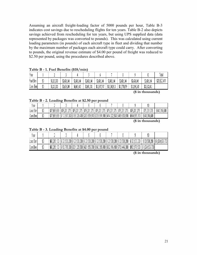
21

Assuming an aircraft freight-loading factor of 5000 pounds per hour, Table B-3indicates cost savings due to rescheduling flights for ten years. Table B-2 also depictssavings achieved from rescheduling for ten years, but using UPS supplied data (datarepresented by packages was converted to pounds). This was calculated using currentloading parameters (in pounds) of each aircraft type in fleet and dividing that numberby the maximum number of packages each aircraft type could carry. After convertingto pounds, the original revenue estimate of $4.00 per pound of freight was reduced to$2.50 per pound, using the procedures described above.

Table B - 1. Fuel Benefits ($18/min)

($ in thousands)

Table B - 2. Loading Benefits at $2.50 per pound

($ in thousands)

Table B - 3. Loading Benefits at $4.00 per pound

($ in thousands)

22

Appendix C: Cash Flow

A: Scenario of fuel $18/min., 10min. dead band, W&E Bank. 5000lb/hr $4 loading Ben/lb, 15% COM, 50% Equipage (in 2 years) Year 1 2 3 4 5 6 7 8 9 10 TotalFuel Ben $0 $1,213,083 $2,426,166 $2,426,166 $2,426,166 $2,426,166 $2,426,166 $2,426,166 $2,426,166 $2,426,166 $20,622,411Cum. Ben $0 $1,213,083 $3,639,249 $6,065,415 $8,491,581 $10,917,747 $13,343,913 $15,770,079 $18,196,245 $20,622,411Load Ben $0 $60,265,100 $120,530,200 $120,530,200 $120,530,200 $120,530,200 $120,530,200 $120,530,200 $120,530,200 $120,530,200 $1,024,506,700Cum.Ben $0 $60,265,100 $180,795,300 $301,325,500 $421,855,700 $542,385,900 $662,916,100 $783,446,300 $903,976,500 $1,024,506,700Total Annu $0 $61,478,183 $122,956,366 $122,956,366 $122,956,366 $122,956,366 $122,956,366 $122,956,366 $122,956,366 $122,956,366 $1,045,129,111Total Cum $0 $61,478,183 $184,434,549 $307,390,915 $430,347,281 $553,303,647 $676,260,013 $799,216,379 $922,172,745 $1,045,129,111Annual Cos$23,442,500 $26,309,125 $6,600,719 $7,556,477 $8,655,598 $9,919,588 $11,373,176 $13,044,802 $14,967,173 $17,177,899 $139,047,056Cum.Cost $23,442,500 $49,751,625 $56,352,344 $63,908,820 $72,564,418 $82,484,006 $93,857,182 $106,901,984 $121,869,157 $139,047,056

Annual NV -$23,442,500 $35,169,058 $116,355,647 $115,399,889 $114,300,768 $113,036,778 $111,583,190 $109,911,564 $107,989,193 $105,778,467 $906,082,055Net PV -$23,442,500 $11,726,558 $128,082,205 $243,482,095 $357,782,863 $470,819,641 $582,402,831 $692,314,395 $800,303,588 $906,082,055

B: Base Case Scenario of fuel $18/min., 10 min. dead band, W&E Bank. 5000lb/hr $2.5 loading Ben/lb, 15% COM, 50% Equipage (in 2 years)Year 1 2 3 4 5 6 7 8 9 10 Total

Fuel Ben $0 $1,213,083 $2,426,166 $2,426,166 $2,426,166 $2,426,166 $2,426,166 $2,426,166 $2,426,166 $2,426,166 $20,622,411Cum. Ben $0 $1,213,083 $3,639,249 $6,065,415 $8,491,581 $10,917,747 $13,343,913 $15,770,079 $18,196,245 $20,622,411Load Ben $0 $37,665,688 $75,331,375 $75,331,375 $75,331,375 $75,331,375 $75,331,375 $75,331,375 $75,331,375 $75,331,375 $640,316,688Cum.Ben $0 $37,665,688 $112,997,063 $188,328,438 $263,659,813 $338,991,188 $414,322,563 $489,653,938 $564,985,313 $640,316,688

tal Annu. Be $0 $38,878,771 $77,757,541 $77,757,541 $77,757,541 $77,757,541 $77,757,541 $77,757,541 $77,757,541 $77,757,541 $660,939,099tal Cum. Be $0 $38,878,771 $116,636,312 $194,393,853 $272,151,394 $349,908,935 $427,666,476 $505,424,017 $583,181,558 $660,939,099Annual Cos $23,442,500 $26,309,125 $6,600,719 $7,556,477 $8,655,598 $9,919,588 $11,373,176 $13,044,802 $14,967,173 $17,177,899 $139,047,056Cum.Cost $23,442,500 $49,751,625 $56,352,344 $63,908,820 $72,564,418 $82,484,006 $93,857,182 $106,901,984 $121,869,157 $139,047,056

Annual NV -$23,442,500 $12,569,646 $71,156,822 $70,201,064 $69,101,943 $67,837,953 $66,384,365 $64,712,739 $62,790,368 $60,579,642 $521,892,043Net PV -$23,442,500 -$10,872,855 $60,283,968 $130,485,032 $199,586,975 $267,424,928 $333,809,293 $398,522,032 $461,312,401 $521,892,043

C: Scenario of fuel $18/min., 10 min. dead band, W&E Bank. 5000lb/hr $4 loading Ben/lb, 9% COM, 50% Equipage (in 2 years)Year 1 2 3 4 5 6 7 8 9 10 Total

Fuel Ben $0 $1,213,083 $2,426,166 $2,426,166 $2,426,166 $2,426,166 $2,426,166 $2,426,166 $2,426,166 $2,426,166 $20,622,411Cum. Ben $0 $1,213,083 $3,639,249 $6,065,415 $8,491,581 $10,917,747 $13,343,913 $15,770,079 $18,196,245 $20,622,411Load Ben $0 $60,265,100 $120,530,200 $120,530,200 $120,530,200 $120,530,200 $120,530,200 $120,530,200 $120,530,200 $120,530,200 $1,024,506,700Cum.Ben $0 $60,265,100 $180,795,300 $301,325,500 $421,855,700 $542,385,900 $662,916,100 $783,446,300 $903,976,500 $1,024,506,700Total Annu $0 $61,478,183 $122,956,366 $122,956,366 $122,956,366 $122,956,366 $122,956,366 $122,956,366 $122,956,366 $122,956,366 $1,045,129,111Total Cum $0 $61,478,183 $184,434,549 $307,390,915 $430,347,281 $553,303,647 $676,260,013 $799,216,379 $922,172,745 $1,045,129,111Annual Cos$22,407,500 $23,999,725 $3,751,035 $4,068,018 $4,413,530 $4,790,138 $5,200,640 $5,648,088 $6,135,806 $6,667,418 $87,081,898Cum.Cost $22,407,500 $46,407,225 $50,158,260 $54,226,279 $58,639,809 $63,429,947 $68,630,587 $74,278,675 $80,414,480 $87,081,898

Annual NV -$22,407,500 $37,478,458 $119,205,331 $118,888,348 $118,542,836 $118,166,228 $117,755,726 $117,308,278 $116,820,560 $116,288,948 $958,047,213Net PV -$22,407,500 $15,070,958 $134,276,289 $253,164,636 $371,707,472 $489,873,700 $607,629,426 $724,937,704 $841,758,265 $958,047,213

D: Scenario of fuel $18/min., 10 min. dead band, W&E Bank. 5000lb/hr $2.5 loading Ben/lb, 9% COM, 50% Equipage (in 2 years)Year 1 2 3 4 5 6 7 8 9 10 TotalFuel Ben $0 $1,213,083 $2,426,166 $2,426,166 $2,426,166 $2,426,166 $2,426,166 $2,426,166 $2,426,166 $2,426,166 $20,622,411Cum. Ben $0 $1,213,083 $3,639,249 $6,065,415 $8,491,581 $10,917,747 $13,343,913 $15,770,079 $18,196,245 $20,622,411Load Ben $0 $37,665,688 $75,331,375 $75,331,375 $75,331,375 $75,331,375 $75,331,375 $75,331,375 $75,331,375 $75,331,375 $640,316,688Cum.Ben $0 $37,665,688 $112,997,063 $188,328,438 $263,659,813 $338,991,188 $414,322,563 $489,653,938 $564,985,313 $640,316,688Total Annu $0 $38,878,771 $77,757,541 $77,757,541 $77,757,541 $77,757,541 $77,757,541 $77,757,541 $77,757,541 $77,757,541 $660,939,099Total Cum $0 $38,878,771 $116,636,312 $194,393,853 $272,151,394 $349,908,935 $427,666,476 $505,424,017 $583,181,558 $660,939,099Annual Cos$22,407,500 $23,999,725 $3,751,035 $4,068,018 $4,413,530 $4,790,138 $5,200,640 $5,648,088 $6,135,806 $6,667,418 $87,081,898Cum.Cost $22,407,500 $46,407,225 $50,158,260 $54,226,279 $58,639,809 $63,429,947 $68,630,587 $74,278,675 $80,414,480 $87,081,898

Annual NV -$22,407,500 $14,879,046 $74,006,506 $73,689,523 $73,344,011 $72,967,403 $72,556,901 $72,109,453 $71,621,735 $71,090,123 $573,857,200Net PV -$22,407,500 -$7,528,455 $66,478,051 $140,167,574 $213,511,585 $286,478,988 $359,035,889 $431,145,342 $502,767,077 $573,857,200

E: Scenario of fuel $18/min., 5 min. dead band, W&E Bank, 5000lb/hr $2.5 loading Ben/lb, 15% COM, 50% Equipage (in 2 years) Year 1 2 3 4 5 6 7 8 9 10 TotalFuel Ben $0 $1,213,083 $2,426,166 $2,426,166 $2,426,166 $2,426,166 $2,426,166 $2,426,166 $2,426,166 $2,426,166 $20,622,411Cum. Ben $0 $1,213,083 $3,639,249 $6,065,415 $8,491,581 $10,917,747 $13,343,913 $15,770,079 $18,196,245 $20,622,411Load Ben $0 $38,403,000 $76,806,000 $76,806,000 $76,806,000 $76,806,000 $76,806,000 $76,806,000 $76,806,000 $76,806,000 $652,851,000Cum.Ben $0 $38,403,000 $115,209,000 $192,015,000 $268,821,000 $345,627,000 $422,433,000 $499,239,000 $576,045,000 $652,851,000Total Annu $0 $39,616,083 $79,232,166 $79,232,166 $79,232,166 $79,232,166 $79,232,166 $79,232,166 $79,232,166 $79,232,166 $673,473,411Total Cum $0 $39,616,083 $118,848,249 $198,080,415 $277,312,581 $356,544,747 $435,776,913 $515,009,079 $594,241,245 $673,473,411Annual Cos$23,442,500 $26,309,125 $6,600,719 $7,556,477 $8,655,598 $9,919,588 $11,373,176 $13,044,802 $14,967,173 $17,177,899 $139,047,056Cum.Cost $23,442,500 $49,751,625 $56,352,344 $63,908,820 $72,564,418 $82,484,006 $93,857,182 $106,901,984 $121,869,157 $139,047,056

Annual NV -$23,442,500 $13,306,958 $72,631,447 $71,675,689 $70,576,568 $69,312,578 $67,858,990 $66,187,364 $64,264,993 $62,054,267 $534,426,355Net PV -$23,442,500 -$10,135,542 $62,495,905 $134,171,595 $204,748,163 $274,060,741 $341,919,731 $408,107,095 $472,372,088 $534,426,355

23

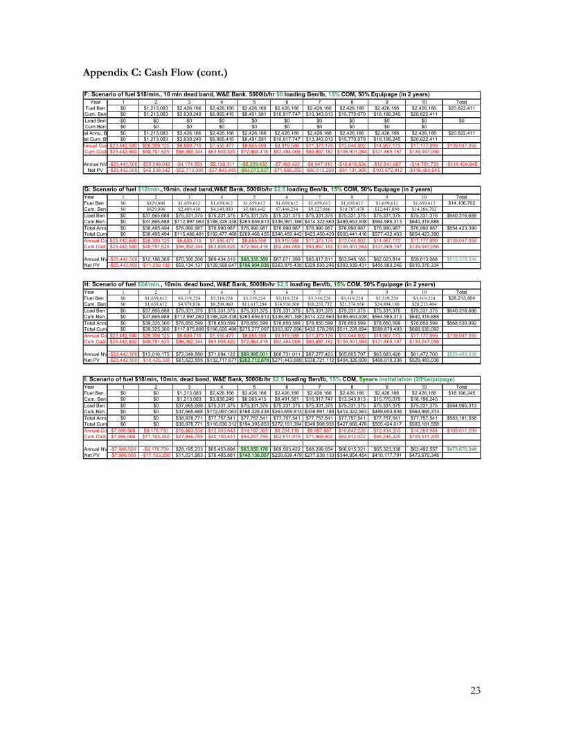
Appendix C: Cash Flow (cont.)

F: Scenario of fuel $18/min., 10 min dead band, W&E Bank. 5000lb/hr $0 loading Ben/lb, 15% COM, 50% Equipage (in 2 years)Year 1 2 3 4 5 6 7 8 9 10 Total

Fuel Ben $0 $1,213,083 $2,426,166 $2,426,166 $2,426,166 $2,426,166 $2,426,166 $2,426,166 $2,426,166 $2,426,166 $20,622,411Cum. Ben $0 $1,213,083 $3,639,249 $6,065,415 $8,491,581 $10,917,747 $13,343,913 $15,770,079 $18,196,245 $20,622,411Load Ben $0 $0 $0 $0 $0 $0 $0 $0 $0 $0 $0Cum.Ben $0 $0 $0 $0 $0 $0 $0 $0 $0 $0

tal Annu. Be $0 $1,213,083 $2,426,166 $2,426,166 $2,426,166 $2,426,166 $2,426,166 $2,426,166 $2,426,166 $2,426,166 $20,622,411tal Cum. Be $0 $1,213,083 $3,639,249 $6,065,415 $8,491,581 $10,917,747 $13,343,913 $15,770,079 $18,196,245 $20,622,411Annual Cos $23,442,500 $26,309,125 $6,600,719 $7,556,477 $8,655,598 $9,919,588 $11,373,176 $13,044,802 $14,967,173 $17,177,899 $139,047,056Cum.Cost $23,442,500 $49,751,625 $56,352,344 $63,908,820 $72,564,418 $82,484,006 $93,857,182 $106,901,984 $121,869,157 $139,047,056

Annual NV -$23,442,500 -$25,096,042 -$4,174,553 -$5,130,311 -$6,229,432 -$7,493,422 -$8,947,010 -$10,618,636 -$12,541,007 -$14,751,733 -$118,424,645Net PV -$23,442,500 -$48,538,542 -$52,713,095 -$57,843,405 -$64,072,837 -$71,566,259 -$80,513,269 -$91,131,905 -$103,672,912 -$118,424,645

G: Scenario of fuel $12/min.,10min. dead band,W&E Bank, 5000lb/hr $2.5 loading Ben/lb, 15% COM, 50% Equipage (in 2 years) Year 1 2 3 4 5 6 7 8 9 10 TotalFuel Ben $0 $829,806 $1,659,612 $1,659,612 $1,659,612 $1,659,612 $1,659,612 $1,659,612 $1,659,612 $1,659,612 $14,106,702Cum. Ben $0 $829,806 $2,489,418 $4,149,030 $5,808,642 $7,468,254 $9,127,866 $10,787,478 $12,447,090 $14,106,702Load Ben $0 $37,665,688 $75,331,375 $75,331,375 $75,331,375 $75,331,375 $75,331,375 $75,331,375 $75,331,375 $75,331,375 $640,316,688Cum.Ben $0 $37,665,688 $112,997,063 $188,328,438 $263,659,813 $338,991,188 $414,322,563 $489,653,938 $564,985,313 $640,316,688Total Annu $0 $38,495,494 $76,990,987 $76,990,987 $76,990,987 $76,990,987 $76,990,987 $76,990,987 $76,990,987 $76,990,987 $654,423,390Total Cum $0 $38,495,494 $115,486,481 $192,477,468 $269,468,455 $346,459,442 $423,450,429 $500,441,416 $577,432,403 $654,423,390Annual Cos$23,442,500 $26,309,125 $6,600,719 $7,556,477 $8,655,598 $9,919,588 $11,373,176 $13,044,802 $14,967,173 $17,177,899 $139,047,056Cum.Cost $23,442,500 $49,751,625 $56,352,344 $63,908,820 $72,564,418 $82,484,006 $93,857,182 $106,901,984 $121,869,157 $139,047,056

Annual NV -$23,442,500 $12,186,369 $70,390,268 $69,434,510 $68,335,389 $67,071,399 $65,617,811 $63,946,185 $62,023,814 $59,813,088 $515,376,334Net PV -$23,442,500 -$11,256,132 $59,134,137 $128,568,647 $196,904,036 $263,975,435 $329,593,246 $393,539,431 $455,563,246 $515,376,334

H: Scenario of fuel $24/min., 10min. dead band, W&E Bank, 5000lb/hr $2.5 loading Ben/lb, 15% COM, 50% Equipage (in 2 years) Year 1 2 3 4 5 6 7 8 9 10 TotalFuel Ben $0 $1,659,612 $3,319,224 $3,319,224 $3,319,224 $3,319,224 $3,319,224 $3,319,224 $3,319,224 $3,319,224 $28,213,404Cum. Ben $0 $1,659,612 $4,978,836 $8,298,060 $11,617,284 $14,936,508 $18,255,732 $21,574,956 $24,894,180 $28,213,404Load Ben $0 $37,665,688 $75,331,375 $75,331,375 $75,331,375 $75,331,375 $75,331,375 $75,331,375 $75,331,375 $75,331,375 $640,316,688Cum.Ben $0 $37,665,688 $112,997,063 $188,328,438 $263,659,813 $338,991,188 $414,322,563 $489,653,938 $564,985,313 $640,316,688Total Annu $0 $39,325,300 $78,650,599 $78,650,599 $78,650,599 $78,650,599 $78,650,599 $78,650,599 $78,650,599 $78,650,599 $668,530,092Total Cum $0 $39,325,300 $117,975,899 $196,626,498 $275,277,097 $353,927,696 $432,578,295 $511,228,894 $589,879,493 $668,530,092Annual Cos$23,442,500 $26,309,125 $6,600,719 $7,556,477 $8,655,598 $9,919,588 $11,373,176 $13,044,802 $14,967,173 $17,177,899 $139,047,056Cum.Cost $23,442,500 $49,751,625 $56,352,344 $63,908,820 $72,564,418 $82,484,006 $93,857,182 $106,901,984 $121,869,157 $139,047,056

Annual NV -$23,442,500 $13,016,175 $72,049,880 $71,094,122 $69,995,001 $68,731,011 $67,277,423 $65,605,797 $63,683,426 $61,472,700 $529,483,036Net PV -$23,442,500 -$10,426,326 $61,623,555 $132,717,677 $202,712,678 $271,443,689 $338,721,112 $404,326,909 $468,010,336 $529,483,036

I: Scenario of fuel $18/min, 10min. dead band, W&E Bank, 5000lb/hr $2.5 loading Ben/lb, 15% COM, 5years insttallation (20%equipage) Year 1 2 3 4 5 6 7 8 9 10 TotalFuel Ben $0 $0 $1,213,083 $2,426,166 $2,426,166 $2,426,166 $2,426,166 $2,426,166 $2,426,166 $2,426,166 $18,196,245Cum. Ben $0 $0 $1,213,083 $3,639,249 $6,065,415 $8,491,581 $10,917,747 $13,343,913 $15,770,079 $18,196,245Load Ben $0 $0 $37,665,688 $75,331,375 $75,331,375 $75,331,375 $75,331,375 $75,331,375 $75,331,375 $75,331,375 $564,985,313Cum.Ben $0 $0 $37,665,688 $112,997,063 $188,328,438 $263,659,813 $338,991,188 $414,322,563 $489,653,938 $564,985,313Total Annu $0 $0 $38,878,771 $77,757,541 $77,757,541 $77,757,541 $77,757,541 $77,757,541 $77,757,541 $77,757,541 $583,181,558Total Cum $0 $0 $38,878,771 $116,636,312 $194,393,853 $272,151,394 $349,908,935 $427,666,476 $505,424,017 $583,181,558Annual Cos $7,986,500 $9,176,750 $10,683,538 $12,303,643 $14,107,365 $8,254,119 $9,457,887 $10,842,220 $12,434,203 $14,264,984 $109,511,209Cum.Cost $7,986,500 $17,163,250 $27,846,788 $40,150,431 $54,257,795 $62,511,915 $71,969,802 $82,812,022 $95,246,225 $109,511,209

Annual NV -$7,986,500 -$9,176,750 $28,195,233 $65,453,898 $63,650,176 $69,503,422 $68,299,654 $66,915,321 $65,323,338 $63,492,557 $473,670,348Net PV -$7,986,500 -$17,163,250 $11,031,983 $76,485,881 $140,136,057 $209,639,479 $277,939,133 $344,854,454 $410,177,791 $473,670,348