THESIS

POTENTIAL INDIRECT EFFECTS OF AEROSOL ON TROPICAL CYCLONE DEVELOPMENT

Submitted by

Geoffrey Krall

Department of Atmospheric Science

In partial fulfillment of the requirements

For the Degree of Master of Science

Colorado State University

Fort Collins, Colorado

Fall 2010

Master’s Committee:

Department Chair: Richard Johnson

Advisor: William Cotton

Sue van den Heever

Richard Eykholt

ii

ABSTRACT

POTENTIAL INDIRECT EFFECTS OF AEROSOL ON TROPICAL CYCLONE DEVELOPMENT

Observational and model evidence suggest that a 2008 Western Pacific typhoon (NURI)

came into contact with and ingested elevated concentrations of aerosol as it neared the

Chinese coast. This study uses a regional model with two-moment bin emulating microphysics

to simulate the typhoon as it enters the field of elevated aerosol concentration. A continental

field of cloud condensation nuclei (CCN) was prescribed based on satellite and global aerosol

model output, then increased for further sensitivity tests. The typhoon was simulated for 96

hours beginning 17 August 2008, the final 60 of which were under varying CCN concentrations

as it neared the Philippines and coastal China. The model was initialized with both global

reanalysis model data and irregularly spaced dropsonde data from a 2008 observational

campaign using an objective analysis routine. At 36 hours, the internal nudging of the model

was switched off and allowed to evolve on its own.

As the typhoon entered the field of elevated CCN in the sensitivity tests, the presence of

additional CCN resulted in a significant perturbation of windspeed, convective fluxes, and

hydrometeor species behavior. Initially ingested in the outer rainbands of the storm, the

additional CCN resulted in an initial damping and subsequent invigoration of convection. The

increase in convective fluxes strongly lag-correlates with increased amounts of supercooled

iii

liquid water within the storm domain. As the convection intensified in the outer rainbands the

storm drifted over the developing cold-pools, affecting the inflow of air into the convective

towers of the typhoon. Changes in the timing and amount of rain produced in each simulation

resulted in differing cold-pool strengths and size. The presence of additional CCN increased

resulted in an amplification of convection within the storm, except for the extremely high CCN

concentration simulation, which showed a damped convection due to the advection of pristine

ice away from the storm. This study examines the physical mechanisms that could potentially

alter a tropical cyclone (TC) in intensity and dynamics upon ingesting elevated levels of CCN.

iv

TABLE OF CONTENTS

Abstract .............................................................................................................................. ii

Table of Contents ............................................................................................................................. iv

Acknowledgements ............................................................................................................................ vi

Chapter 1 - Introduction

1.1 Aerosol Theory and Droplet Growth ............................................................................... 1

1.2 Aerosol Sources and Spatial Distribution in and Around China ...................................... 4

1.3 TCs and TC Formation Theory ......................................................................................... 7

1.4 TC-Aerosol Interaction..................................................................................................... 9

1.5 Objective of Research…. ................................................................................................12

1.6 DoD Relevance ..............................................................................................................13

1.7 Chapter 1 Figures ..........................................................................................................15

Chapter 2 – The RAMS Model

2.1 RAMS 4.3: The Microphysical Scheme ..........................................................................16

2.2 ISAN (ISentropic ANalysis) Processing and the Barnes Scheme ...................................19

2.3 Past RAMS-TC Experiments ...........................................................................................19

Chapter 3 – T-PARC and TC NURI

3.1 The T-PARC Campaign ...................................................................................................23

3.2 Dropsonde Data ............................................................................................................24

3.3 TC NURI .......................................................................................................................24

3.4 Chapter 3 Figures ..........................................................................................................27

v

Chapter 4 – Model Configuration and Control Simulation

4.1 Grid Configuration .........................................................................................................29

4.2 Model Initialization .......................................................................................................30

4.3 Aerosol Prescription ......................................................................................................31

4.4 Discussion of Control Simulation Results ......................................................................33

4.5 Chapter 4 Tables and Figures ........................................................................................35

Chapter 5 - Results

5.1 General Discussion ........................................................................................................47

5.2 Precipitation Modulation and Convective Activity ........................................................49

5.3 Downward Flux ..............................................................................................................52

5.4 Cold-pool Parameters ....................................................................................................56

5.5 Response of Hydrometeors ...........................................................................................60

5.6 Chapter 5 Figures ..........................................................................................................65

Chapter 6 - Conclusions

6.1 Summary of Study .........................................................................................................97

6.2 TC Windspeed and Track ...............................................................................................98

6.3 Droplet size, SCLW, and Convective Fluxes ....................................................................98

6.4 Cold-pool Modulation ...................................................................................................99

6.5 Two Potential Routes of CCN to Weaken a Storm .......................................................100

6.6 A Comment on the Importance of Microphysics in TC Forecasting and

Predicting ....................................................................................................................101

6.7 Recommendations for Future Work ............................................................................102

6.8 Chapter 6 Figures ........................................................................................................104

References ......................................................................................................................... 105

vi

ACKNOWLEDGEMENTS

There are too many persons who helped and supported me over the course of my Masters work at CSU

to recount. Nevertheless I will try.

Particular thanks is reserved for my advisor and personal trainer Dr. William Cotton, who plucked me

seemingly out of thin air and gave me an excuse to move from Texas to Colorado; for that I and my

family are grateful. I am indebted to the entire Cotton group, past and present. Every single member

offered encouragement, helped me troubleshoot, and helped me better understand how the

atmosphere worked; in particular, Dan Ward, who was easily the best TA I had at CSU, Stephen Saleeby,

who was my go-to guy for any questions I had about anything, and Gustavo Carrio – I hope my

assistance with the English language made up for your assistance with the only slightly less

understandable atmosphere. I would like to thank my committee member Dr. Sue van den Heever for

continuing to give advice to a student, long after I completed AT540. I would also like to thank Professor

Dr. Tom Vonder Haar, Andy Jones and the entire CG/AR community for their support - the annual review

sessions and ongoing conversations helped hone my research and ability as a scientist. Thanks to Nick

Guy and his beautiful family: it was crucial to find someone else who knows the trials and tribulations

brought on by a lack of caffeine, rooting for terrible football teams, and obtaining an advanced degree

vii

while rearing small children. I would like to thank Omar Little for his sage words of wisdom. I would also

like to extend my deepest gratitude to my parents, Ed and Lee Krall, for their continued support in my

ongoing endeavors and instilling in me a love for education and science.

My research could not have taken place without the selfless childcare provided by my mother-in-law,

Natalie Kimble and her husband Donald. To my indefatigable daughter and son, Adeline and Jude, I can

only hope that your lives have been made more adventurous by our move to Colorado. Thank you for

always being excited to see me at the end of the day. Your unrelenting joy is a cool drink of water. And

lastly, to my best friend and wife, Stephanie, thank you for simultaneously challenging me, encouraging

me, and for continuing to make me laugh decade after decade.

This research was made possible by funding from CG/AR and the Department of Defense.

1

Chapter 1 CHAPTER 1 – INTRODUCTION

1.1: Aerosol Theory and Droplet Growth

Aerosols are tiny particles that exist or are emitted into the atmosphere through natural and

anthropogenic processes. These particles have the potential to alter both weather and climate

patterns through modulating the earth's radiation budget and by perturbing the water cycle

upon their interaction with water vapor. These processes are among the most difficult to

quantify on a global scale as the sources, species, quantity, and effect of aerosols vary wildly

throughout the globe; they are difficult to track with certainty. However, due to their weather

and climate altering potential, research into aerosol effects has expanded in recent years.

When a particle travels through air with a certain amount of water vapor, the particle may have

the ability to develop tiny water drops on its surface. Absent the introduction of aerosols, water

vapor may only convert into water droplets by homogeneous nucleation, which requires very

low temperatures and/or unrealistic levels of supersaturation. The introduction of aerosol acts

to facilitate the development of the initial droplet in air. The aerosol at this point acts as cloud

condensation nuclei (CCN) and allows liquid water to form from water vapor at lower values of

supersaturation and higher temperatures. The ability of an aerosol particle to act as CCN is a

2

function of both its size and chemical species. These variables work to control the hydroscopicity

which determines the particle's ability to take on water, although Dusek et al. (2006) provided

evidence that a particle's ability to nucleate droplets was more affected by size: the larger the

particle, the greater the ability to activate cloud droplets.

At this point, the microscopic water molecule may grow. Kohler (1926) determined the

equilibrium vapor pressure above small droplets. This allowed him to develop what are now

known as the Kohler curves. They yield a size threshold of droplet growth according to the

supersaturation of the air with respect to water vapor. Given a water droplet and

supersaturation, the droplet may either remain at its size as a stable water droplet if it does not

pass that prescribed threshold or it may continue to grow once it surpasses a certain size and

supersaturation. The droplet at this point will continue to grow indefinitely until it is rained out

or broken up in some other manner. The droplet may also evaporate if forced in the opposite

direction. This basic model of droplet initialization, growth, and fallout is the prevalent model of

precipitation. Because these processes occur on the microscopic scale, atmospheric models are

burdened with the challenge of representing this process in a dynamic system countless times

without utilizing an unrealistic amount of computing power.

Howell (1949) was the first to discuss CCN quantitatively. He noted that the observed size

spectra of water droplets were much broader than would be predicted theoretically. Twomey

and Squires (1959) were among the first to attempt to obtain an observed concentration of CCN

by measuring the spectrum of critical supersaturation of cloud nuclei (CN) in the air beneath a

cumulus cloud as well as the droplet concentration within the cloud. Volkovitsky and Laktionov

3

(1969) utilized a 3000 m3 cloud chamber to obtain a droplet spectrum according to various

temperatures.

As global anthropogenic emission of aerosols have increased over the past several decades

(Streets et al. 2000; Streets and Waldhoff 2000) aerosol effects are at the forefront of advertent

and inadvertent weather modification research. As such, aerosol effects have been well-

categorized. They have been shown to be direct scatterers of radiation (Charlson et al. 1992)

and direct absorbers (Ramanathan and Vogelmann 1997). In addition, aerosols have been

shown to affect precipitation. If water vapor is considered constant, the introduction of more

CCN would imply that the nascent water droplets would be smaller and therefore inhibit the

collision-coalescence process. While CCN are critical to the formation of droplets, in the

presence of high concentrations of CCN, water droplets may be unable to grow large enough to

precipitate out of a cloud. This phenomenon and its consequences have been documented as

so-called indirect effects. The first indirect effect (Twomey 1991) suggests that given the same

liquid water content (LWC) additional CCN may act to increase the number droplet

concentration and increase cloud albedo. The second indirect effect (Albrecht 1989), or lifetime

effect, suggests in the presence of heightened CCN concentration clouds will be less able to

precipitate out their moisture, thereby lengthening the lifetime of the cloud. This effect is

primarily attributed to stratocumulus clouds.

Aerosol induced precipitation changes do not generally have such a linear response. Modeling

studies suggest that in certain types of precipitating regimes, in particular convectively driven

systems, CCN may work to enhance precipitation intensity. While additional CCN may initially

inhibit precipitation, over the course of a storm the smaller droplets, unable to rain out, are

4

lifted in an updraft; this causes the latent heat release due to freezing droplets in the

atmosphere to significantly increase the vertical velocity and amplify the storm (van den Heever

et al. 2006; Seifert and Beheng 2006). The nonlinear response of precipitation to aerosols

provides a wealth of research opportunities.

1.2: Aerosol Sources and Spatial Distribution in and Around China

Providing a global survey of aerosol concentrations is challenging due to their small size,

tendency to react chemically, and not being a purely surface emission process. In addition to

being emitted at the surface, aerosol particles may form in the atmosphere itself via gas-to-

particle (GTP) conversion. Taking chemical composition into account provides another level of

complexity as aerosol particles may change chemically by interacting with other particles or

solar radiation. For the purposes of this research, three general types of contributing aerosols

are considered: soil and mineral dust, sea salt, and anthropogenic particles.

Among the most prevalent natural source of aerosols is soil and mineral dust (Duce 1995),

sourced primarily from large, arid deserts. Tegen (2003) and Zender et al. (2004) well summarize

the most recent research into estimates of soil and mineral dust concentrations globally. Dust is

of particular interest due to its composition: often it is made up of soluble materials that render

the dust particles highly suitable as CCN (Formenti et al. 2003) and ice nuclei (IN) (DeMott et al.

2003; Twohey et al. 2009). Strong winds blown over a dust source can quickly generate

extremely high concentrations of dust near the surface (Cheng et al. 2004). Once the larger dust

particles have been scavenged or sedimented out, the remaining smaller dust particles can

travel thousands of kilometers horizontally and several kilometers vertically. Saharan dust

regularly advects westward across the Atlantic ocean into the southeastern continental United

5

States. The Gobi desert meanwhile is under siege by westerly winds, carrying particles into and

across the Pacific Ocean. The frequency and intensity of these major dust events is exacerbated

under dry or drought conditions.

Sea salt is also a suitable CCN. Sea salt particles are emitted to the atmosphere when air bubbles

rise to the ocean surface and burst during whitecap formation (Schulz et al. 2004). In maritime

environments sea salt is often the dominant source of aerosols. Since the formation of sea salt

particles is directly linked to whitecap formation, it stands to reason that there is a direct

correlation between surface windspeed and sea salt aerosol concentration just as in dust

aerosols. Sea salt can have a wide size distribution spectrum (from 0.05 to 10 microns in

diameter; Leinert et al. 2003) and therefore has been implicated in affecting warm rain

processes in marine environments (Jensen and Lee 2008).

While dust and sea salt particles dominate the natural influencing aerosols for the purposes of

this study, anthropogenic aerosols in and around China are also strongly considered due to their

potential for interaction with tropical storms (TSs). From 1980 to 1990, China saw a 60%

increase in sulfur dioxide (Streets et al. 2000). This was a result of a sharp population increase,

rapid economic growth, and an increased dependence on coal. Similarly, throughout the 1990's

China's SO2 emissions increased by an average of 3.6% a year (Streets and Waldhoff 2000).

Satellite retrievals have suggested a decadal increase in aerosol optical depth (AOD) of about

17% over the China coastal plain (Massie et al. 2004). More recently - thanks to technological

advances in energy production, a lessened emphasis on coal, and an emphasis on pollution

capturing - Asian SO2 emissions have declined from 38.5 Tg in 1995 to 34.4 Tg in 2000, a

6

decrease of 2.3% a year (Carmichael et al. 2002).

SO2 is the dominant player for anthropogenic aerosol compounds in the region. Once aloft, SO2

can oxidize into sulfate aerosol particles (Saxena and Seignuer 1987). Berglen et al. (2004)

estimated between 51 and 56% of SO2 gets converted to sulfate into the atmosphere. Globally,

sulfates dominate number load of anthropogenic aerosols for now and into the foreseeable

future (Dentener et al. 2006).

The vertical distribution of aerosols in and around China is also considered. Observational

studies have shown that dust, which dominates the coarse mode of aerosol exists throughout a

vertical column while pollution generated aerosol, which dominate the accumulation mode of

aerosol, are generally confined near the boundary layer (Anderson et al. 2003a; Chin et al.

2003). However, the dust aerosol advecting out of Asia over the ocean shows a tendency to

contain layers of particles separated by layers of relatively clean atmosphere often 2-4 km

above ground level (Redemann et al. 2003; Bahreini et al. 2003) .

These three types of aerosol are considered in this study as the dominant regional aerosol

modes in China and the Western Pacific insofar as weather and climate modification. As noted

by Dusek et al. (2006), the chemical makeup of the aerosol constituents is of secondary concern

relative to number concentration and size. Unable to examine every aerosol species available,

the primary aerosol focus of this study is on number concentration and size. Therefore, we

utilize observational studies, in-situ measurements, and satellite retrievals that do not

necessarily distinguish between aerosol species.

7

1.3: TCs and TC Formation Theory

Few weather events attract as much research as landfalling tropical cyclones (TCs) thanks to

their high destructive potential, a life cycle that allows for intensification, deintensification,

sudden track shifts, and the countless meteorological variables that may affect a particular

storm. Characterized by a low-pressure system center, tropical depressions (TDs), tropical

storms (TSs), and TCs are fueled by warm ocean water vapor and the associated deep

convection latent heat release, distinguishing it from mid-latitude cyclones which are driven by a

preexisting horizontal temperature gradient. The deep convection associated with a TS requires

a constant supply of moisture and therefore deintensify rapidly upon reaching land. Still, a

strong TC can still remain active thousands of kilometers inland, spawning tornadoes (Novlan

and Gray 1974; Gentry 1983; McCaul 1991), thunderstorms, and flooding from rainfall and

storm surges (Crawford 1979) for days after making landfall.

While TC forecasting has improved dramatically over the past several decades in terms of track

and intensity (Willoughby et al. 1982; Emanuel 1986,1988; Willoughby 1990a, b, 1998, Powell

1990a, b; Gray 1995; Shapiro and Franklin 1999; Braun and Tao 2000; Wang 2002a; Zhu and

Smith 2002; McFarquhar and Black 2004; Zhu and Zhang 2006; Rogers et al. 2007), there is still

considerable uncertainty when it comes to TC genesis and TC response to anthropogenic forcing

(Bender et al. 2010). Furthermore, while TC forecasts have improved significantly, there still

remains enough uncertainty that improvements in track and intensity forecasting could greatly

benefit regions of high TC landfalling activity, particularly regions close to sea level.

Tropical cyclogenesis has been a subject of great debate in the atmospheric science community

for decades since Reihl and Malkus's (1958) pioneering work noting the role of convectively-

8

generated hot towers in TC formation. From this work came the most cited theory of tropical

cyclone formation of the subsequent decades - conditional instability of the second kind, or

CISK, as described by Ooyama (1964) and Charney and Elliasson (1964). CISK assumes a

destabilization of the atmosphere driven by organized moist convection due to surface fluxes

and radiation fluxes. A competing, though not mutually exclusive, alternative theory to TC

formation began to emerge in the mid-1980s, introduced by Emanuel (1986) as air-sea

interaction instability (ASII), subsequently renamed wind-induced surface heat exchange, or

WISHE, instability (Emanuel et al. 1994). In the WISHE model, the convective instability is

generated by a feedback mechanism from surface fluxes of heat and moisture dependent on

windspeed derived from a preexisting vortex. The primary difference between the two theories

can be seen as their dependence on convective available potential energy (CAPE). An implication

of CISK theory is that TC genesis must be accompanied by a positive amount of CAPE, while

according to WISHE, the atmosphere may be initially convectively neutral and therefore TC

genesis may occur when CAPE is zero. Recent modeling studies (e.g. Craig and Gray 1996) have

tended to support the potential for TC formation in a zero CAPE atmosphere. However, the

CISK-WISHE debate was of paramount importance in our understanding of TC development in

terms of convective fluxes.

Of particular value in the CISK-WISHE debate was the increased attention given to convectively-

generated downdrafts in TC formation. Zipser (1977) described the importance of downdrafts in

convective systems, while Simpson (1980) proposed these downdrafts could initiate future

convection. Other studies (e.g. Thorpe et al. 1982; Rotunno et al. 1988) directly implicated

surface-based cold pools as a crucial factor in organizing deep convection. Emanuel (1994) cited

the lifting of the boundary layer (BL) at cold-pool front through its negatively buoyant

9

convective inhibition layer, allowing free convection to commence as a method to convection

organization. Mapes (2000) extended this in a toy tropical model. Tompkins (2001) observed

that new convective events were being initiated on the boundaries of cold-pools emanating

from previous cumulus towers. Due to the intense convection in a TC, lightning has been used

recently to link TC activity and latent heat release (Lyons and Keen 1994; Orville and Coyne

1999, Molinari et al 1999; Shao et al. 2005; Fierro et al. 2007, Price et al. 2009). Other factors in

TC formation include vertical wind shear, assumed to have a negative impact on TC

development (Rotunno et al. 1998; LeMone et al. 1998), gravity waves (Mapes 1993). Recently

much attention has been focused on the bottom-up development of near-eye vortical hot

towers (Montgomery and Enagonio 1998; Hendricks et al. 2004; Montgomery et al. 2006) as a

potential route to cyclogenesis.

This study will focus much of its attention on the cold-pools generated within a TC due to latent

heat release and convective fluxes.

1.4: TC-Aerosol Interaction

The origins of microphysical impacts on TC development stem from project STORMFURY from

1962 to 1983.During this lengthy campaign, TC rainbands were seeded with silver iodide. The

hypothesis was that the silver iodide, also used in cloud seeding experiments during this time,

would enhance thunderstorms along the outer rainbands of the storm, which would in turn

compete with the eyewall by damping convergence (Simpson and Malkus, 1964). Despite some

initially promising results, the success of STORMFURY came into question in the mid-1980s as it

became apparent that it was impossible to distinguish the effects of the seeding with natural

processes (Willoughby et al. 1985). At this time there was still a considerable lack of

10

understanding of microphysical processes involved in rain formation, droplet growth, and the

resultant perturbation in latent heat release.

While the results of STORMFURY may have been questionable, the idea that microphysical

processes could potentially alter and hopefully mitigate storm damage is gaining strength in the

atmospheric modeling community (Khain et al. 2009; Carrio and Cotton 2010). With increased

computing power and more intricate models that include a fuller microphysics scheme than

previously possible, research on particle-TC interaction is experiencing a reinvigoration.

Of particular interest is the importance of CCN induced cold-pool activity. Wang (2002)

concluded that downdrafts emanating from a TD’s peripheral spiral rain bands acted to hinder

BL convergence at the eyewall. The cold-pool downdraft front can potentially act to cut off the

inflow of warm, near sea-surface air, requisite in maintaining the energetics of the system.

Wang (2009) proposed a relatively linear association between outer rain band activity and TC

intensity: heating the outer rainbands decreases TC intensity by breaking down the

thermodynamic structure of the storm by inducing shear, while cooling the rainbands increases

TC intensity. While it is hard to imagine the relationship being so simple, the impetus to conduct

further modeling and observational studies relating rainband activity and TC intensity is evident.

Based on studies that have shown significant aerosol impacts on cold- pool downdrafts (e.g. van

den Heever and Cotton 2007), the question may be posited: if increased aerosol concentration

may strengthen the downdrafts in a convective storm, could increased aerosol concentration

also amplify the downdrafts in the convective bands in a TC? Should the downdrafts prove to be

strong enough, they could work to damp the BL inflow of warm, moist air which drives the TC.

11

Recent studies have addressed this question largely by examining Atlantic Hurricanes that

entrain dust from the Saharan Desert. Saharan dust is prevalent during the Atlantic hurricane

season, carried for thousands of kilometers on consistent easterly winds. As previously

mentioned, desert dust may act as CCN, which would possibly affect the convection occurring in

the outer rainbands of an existing TC. Zhang et al. (2007;2009) used an idealized simulation of a

TC entraining CCN, showing that the increased aerosol concentration worked to damp the

intensity of the hurricane while increasing its size, consistent with Wang (2009). The aerosols in

such an instance are carried within the Saharan Air Layer (SAL), an exceptionally dry and stable

layer of air which may be of as much importance in suppressing Atlantic TC activity as the

aerosols themselves (Dunion and Velden 2004). It is also possible that the radiative properties of

the dust within the SAL may perturb the atmospheric energy balance and work to weaken TSs

(Evan et al. 2006). A schematic diagram of TC energetics being hindered by a CCN-induced cold-

pool is shown for clarity in Figure 1.1.

Khain et al. (2009), using the Weather Research and Forecasting (WRF) model with spectral bin

microphysics concluded that the entrainment of continental aerosols acted to weaken hurricane

Katrina (2005) just before it made landfall. As noted in Fovell et al. (2009), the microphysics

scheme used in the research model, along with the differences in particle fall speed and how

various species of water vapor are handled, may greatly affect the results. Therefore, as

research on aerosol induced changes in TC intensity is reinvigorated, there must be a wealth of

both modeling and observational studies to corroborate any prevailing theory.

12

1.5: Objective of Research

The primary objective of this research is to determine the indirect effects of aerosols on TC

development. As indicated in previously, there have been many studies examining the effects of

aerosols on TCs, often in the context of dust particles contained within the SAL, which makes it

difficult to distinguish between the aerosol effects and the effects of a dry, stable air layer being

entrained within a TC as a means to deintensification. For this reason, this research will focus on

TC development in the Western Pacific (WP), where aerosol contributions are significant and

carried in an atmosphere similar to the large scale environment. As discussed earlier in this

chapter, both natural and anthropogenic sources of aerosols are present in the WP. A TC case

study was selected for both its wealth of observational data and its assumed interaction with

aerosol particles emanating from the East Asian coast.

In order to best represent the microphysical processes potentially involved in TC modulation, a

regional model with a bin emulating microphysics scheme was implemented. By running

sensitivity tests with various aerosol concentrations, this research allows for a teasing out of the

indirect effects that could potentially modulate and perhaps mitigate the intensity of TCs.

Particular attention is given to the development and modulation of cold-pool activity. This is

achieved by examining rainfall rates in the outer bands of the TC, buoyancy (Emmanuel 1994),

perturbations in equivalent potential temperature ( ) and vertical velocity (w). Attention is also

given to the variation in TC track, maximum and average windspeed, and perturbation pressure.

The final section in this chapter addresses the relevance to the Department of Defense (DoD),

whose collaboration with the Center for Geosciences/Atmospheric Research (CG/AR) worked to

fund this research. A description of the regional model with particular emphasis on the

13

development of the microphysical scheme of the model used is presented in chapter 2. A

background of the TC case study selected and observational campaign used to assist the

initialization of the model assess the quality of the model results is presented in chapter 3.

Chapter 4 contains a detailed description of the model experiment and a discussion of the

control results. Chapter 5 focuses on the subsequent sensitivity tests run assessing the aerosol

induced perturbations on the TC. A summary of the research, along with pertinent conclusions

and suggestions for future TC-aerosol research, is given in chapter 6.

Chapter 1.6: DoD Relevance

The United States Military continues to maintain a presence in the WP for reconnaissance,

research, and relief purposes. The Naval Research Laboratory (NRL) has been particularly

interested in improving the forecast of intensity, structure, and track of TCs (Reynolds et al.

2009) by improving the Coupled Ocean/Atmosphere Mesoscale Prediction System (COAMPS)

and the Navy Operational Global Atmosphere Prediction System (NOGAPS). To do this, the NRL

has collaborated with the Navy and US Air Force to conduct research field campaigns, most

recently in the Western Pacific studying typhoons.

NRL has shown a commitment to atmospheric research for decades and helped to fund this

work. Past DoD funded research has included the development and implementation of a more

accurate CCN advection scheme within the regional model used in this study (Smith 2008). The

DoD has also funded the inclusion of a direct radiative scheme within the regional model

(Stokowski 2005).

14

The Navy continues to be active in providing relief in the form of food, supplies and labor in the

aftermath of a WP typhoon. This research will potentially improve the forecasting of TCs by

including microphysical effects in their predictions, thus giving communities more time to

evacuate or prepare for storms.

15

1.7: Chapter 1 Figures

Figure 1.1: A schematic diagram showing the potential for CCN to hinder TC energetics. After initially suppressing precipitation in the outer rainbands, the additional CCN acts to reduce droplet size and increase amount of supercooled liquid water. As the supercooled liquid water freezes the enhanced latent heat release also enhances convection, which could in turn produce stronger downdrafts and cold-pools. The cold-pools may then work to suppress the warm, moist air entraining into the system.

16

Chapter 2 CHAPTER 2 – THE RAMS MODEL

2.1: RAMS 4.3: the Microphysical Scheme

This study used the Regional Atmospheric Modeling System (RAMS). Being quite malleable in

terms of regional modeling and containing an advanced microphysics scheme, the use of RAMS

provides unique insight on aerosol interaction with various types of precipitation and cloud

formation, even including convective storms and TSs.

Originally developed at Colorado State University (CSU), RAMS has undergone multiple updates

and now exists in over 100 iterations throughout the world. It has been used to simulate a wide

range of atmospheric situations, from large scale dynamics to boundary layer eddies and wind

advecting around individual buildings to microscale wind tunnel simulations (Cotton et al. 2003).

Primarily it is used to simulate atmospheric phenomena on the synoptic or mesoscale.

For this study version 4.3 of RAMS was used. It utilizes an Arakawa-C grid structure (Arakawa and

Lamb, 1981; Randall, 1984) with the option for multiple two-way nested grids and the ability to

add and subtract the nested grids within a simulation. The domain follows a rotated polar-

stereographic transformation horizontally and a terrain-following coordinate system vertically. A

17

non-hydrostatic model, RAMS prognoses 14 variables: u, v, and, w wind components, ice-liquid

water potential temperature, dry air density, total water mixing ratio and eight hydrometeor

species. The radiation is calculated according to the Harrington (1997) long/shortwave model.

The model includes a Kain-Fritsch convective parameterization. The boundary conditions allow

for user-prescribed nudging time-scales. Much of the background information of RAMS can be

found in Cotton et al. (2003). The remainder of this section will focus on the microphysical

developments RAMS has undergone.

The inception of the RAMS model occurred in the early 1980’s with a merger of three separate

but related models: the sea breeze model as described by Mahrer and Pielke (1977), the CSU

cloud model (Tripoli and Cotton 1980), and a hydrostatic version of the cloud model (Tremback

1990). The original “alpha”-version of RAMS had to be extremely constrained due to the limited

computing resources at the time. Eventually as computing power increased, RAMS was released

in 1988 as version 0a with the rewriting of much of the original RAMS code and the inclusion of

parameterizations from the sea breeze model. Critical to the advancement of RAMS was its

ability to take advantage of parallel computing thanks to the calculation of many of the variables

locally, rather than globally. As such, the use of RAMS, widely distributed as version 2c in 1991,

grew throughout the 1990’s.

For this study, there is an inherent focus on microphysical and hydrometeorological processes.

The first microphysics scheme, published in Cotton (1972a, b) was used for investigations into

lake effect storms. The introduction of an ice crystal class of hydrometeors is described in Cotton

(1982) and Cotton et al. (1986). Later, Verlinde et al. (1990) showed that solutions to the full

stochastic collection equation can be obtained using approximations to the collection

18

efficiencies. The implementation of this allowance for prediction of mixing ratios of

hydrometeors within RAMS is described in Walko et al. (1995). This was achieved by using a

single-moment Gamma distribution of all hydrometeor species as the approximation. The

solutions of the full stochastic equations were constructed into a set of look-up tables that

allowed for fast and accurate implementation of the stochastic equations within RAMS. At this

time the development of the RAMS ice nucleation scheme began to include homogeneous

nucleation of ice from haze particles and cloud droplets. Meyers et al. (1997) extended this

approach to include a second moment: mass concentration of the hydrometeor species.

Feingold et al. (1998) advanced the use of the look-up tables by using realistic collection kernels

and implementing a bin-emulating scheme by dividing the gamma distribution into discrete bins.

The bin emulating approach also allowed for the sedimentation of hydrometeor species. Saleeby

and Cotton (2004a, b) developed the inclusion of a large-mode for water droplets (40-80

microns). This effectively allowed for now eight hydrometeor species: small cloud droplets, large

cloud droplets, rain, pristine ice, snow, aggregates, graupel, and hail.

The treatment and adjustment of CCN in RAMS will be the primary motivation of the sensitivity

study of this research. The cloud droplet number is derived from a prognosed CCN field. The

number of CCN that activate is a function of temperature, supersaturation, vertical velocity, and

CCN concentration as determined by a series of look-up tables previously generated offline in a

parcel model run (Saleeby and Cotton 2004) . Currently, activation according to chemistry is fixed

(along with mean radius) for a given simulation, currently as ammonium sulfate. Recently, Ward

et al. (2010) has investigated the inclusion of the kappa parameter as described in Petters and

Kreidenweis (2007). Ward et al. (2010) demonstrated it can be included in RAMS simulations

using an expanded look-up table. The CCN field is initially user-prescribed and may be advected,

19

consumed via activation, and/or diffused by the model.

2.2: ISAN (ISentropic ANalysis) Processing and the Barnes Scheme

For this research, a specific TS case study is utilized. We take advantage of the availability of both

the model reanalysis data and specific dropsondes from the TC case study examined to assist in

the initialization of the simulation. RAMS allows for both gridded data and irregularly spaced

point data to be implemented in the initialization via ISAN processing and the Barnes Scheme.

The ISAN processing is a routine that interpolates gridded data into the user-prescribed grid

domain (Tremback 1990). The Barnes scheme (Barnes 1973) is an objective analysis routine that

incorporates point data as well such as soundings from rawindsondes, dropsondes, etc., where

available.

The Barnes scheme allows for the user to define the strength of the point data versus the

gridded data processed by the ISAN routine. Typically the Barnes scheme is implemented with a

point data weight of 10 to 1000 times stronger than the gridded data. The routine band-passes

the data and applies a smoothing according to two user-prescribed parameters: the wavelength

of the data on the isentropic and upper air surfaces and the fractional amplitude at which to

retain that wavelength. Both the ISAN and Barnes routines construct fixed initialization grids and

nudging varfiles according to the following recorded atmospheric parameters: u and v wind,

temperature, geopotential height, and relative humidity.

2.3: Past RAMS-TC Experiments

RAMS has been used to simulate TCs in the past, albeit sparsely. Due to the high windspeeds, the

20

resolution required to sufficiently simulate a TC is rather fine such that a parcel of air may be

advected over no more than a single grid space in a given time step, while the large scale

meteorology must also be well represented. For this reason a nested grid scheme is ubiquitous

in all RAMS-TC simulations.

Nicholls and Pielke (1995) used a nested grid scheme with a fine grid resolution of 4 km. A

horizontally homogeneous Jordan (1958) sounding based on typical Atlantic hurricane conditions

was used. The authors noted a realistic structure including spiral bands, a clear eye, and a radius

of maximum wind that sloped with height. Upon spin-up, a maximum windspeed of 20 m/s was

achieved 40 km from TC center. Eastman (1995) used RAMS to simulate hurricane Andrew via

National Meteorological Center (NMC) gridded pressure data, upper air rawindsonde data

observations, and a bogus vortex in gradient wind balance.

More recently Montgomery et al. (2006) investigated the role of vortical hot towers in idealized

TC simulations with RAMS. This code utilized a balanced vortex initialization method and has

been used extensively to investigate the dynamics of TCs. In particular Zhang (2007, 2009)

investigated the impacts of African dust acting as CCN on Atlantic hurricanes in a series of

idealized simulations. Those studies revealed a non-monotonic impact of CCN on TC intensity.

While initial increases in CCN concentrations decreased the strength of the storm, higher

concentrations had little impact, often even increasing the strength of the storm. The size of the

storm was also affected, with the highest CCN concentrations yielding the most widespread

storm.

Carrio and Cotton (2010) further investigated CCN impact on hurricanes by using RAMS to

21

simulate the seeding of a TC with extremely high concentrations of CCN within the outer

rainbands of the storm. Those experiments yielded a smaller mean cloud droplet radius within

the cloud bands leading to elevated levels of supercooled water and higher levels of latent heat

released due to freezing. The resultant cold-pools were then stronger and more widespread

under higher CCN concentrations. This acted to interfere with the inflow of moisture into the

convective regions, acting to suppress the storm. The impact of very high CCN concentrations on

riming on ice particles was also evident. Due to the extremely small hydrometeor size, very high

CCN concentrations led to reduced riming and collision-coalescence and thus greater transport

of pristine ice into the anvils of the storm rather than being precipitated to the surface.

Also potentially suppressing the strength of the storm is the act of initiating more disorganized

convective fluxes, upward and downward, leading to greater asymmetrical heating as described

in Nolan et al. (2007). An increase of shear indirectly caused by the ingestion of higher

concentrations of CCN altering the latent heat profile and amplifying downdraft currents, would

lead to the intrusion of low air into the convective towers near the eye and act to inhibit

storm development (Reimer et al 2010).

In most RAMS simulations the Atlantic Jordan (1958) mean sounding has been used as the initial

gridded wind and thermodynamic fields. The impacts of dust carried within the SAL have been

investigated as the primary source of aerosol (Zhang et al. 2007, 2009). Among the features of

the SAL, as indicated in Chapter 1, is a uniquely dry, stable layer, probably modulating a TC

directly rather than taking microphysical effects into account.

To best understand the microphysical effects on TC development, a case study from the Western

22

Pacific (WP) was used. As discussed in Chapter 1, the aerosol-containing air from the WP is not

dissimilar from a TC’s large scale environment *need reference+. In the next chapter we describe

the case study TC and field campaign used to guide and evaluate the RAMS model simulations.

Chapter 4 contains a table summarizing many of the RAMS options available and those chosen

for this experiment.

23

Chapter 3 CHAPTER 3 - THE T-PARC CAMPAIGN AND

TC NURI

3.1. The T-PARC Campaign

In 2008, an ambitious multi-national field campaign was conducted in the Western Pacific in

part to better forecast high-impact weather events. THe Observing Research and Predictability

EXperiment (THORPEX) Pacific Asian Regional Campaign (T-PARC) was a joint effort between the

U.S. DoD-based Naval Research Laboratory, the National Science Foundation (NSF), the Japan

Meteorological Agency, and several other institutions. The general scientific objectives were to

better understand the route to tropical cyclogenesis and the implicit structure changes TCs

undergo. In particular, there was an emphasis on parsing out the difference in synoptic versus

mesoscale influences in the intensification and structure evolution of a TC.

To do this, T-PARC employed the use of several aircraft and ships from August 1 to September

30 collecting observational data in the form of dropsondes, ship-boarded radar, air-borne lidar,

microwave radiometer, and satellite observations as well as the model forecasts from

approximately seven weather centers.

24

3.2 Dropsonde Data

Witnessing several named typhoons, the T-PARC campaign had four aircraft at their disposal,

each equipped with dropsonde drop capabilities. For the TC used for this case study the U.S. Air

Force (AF) C-130 was the primary agent of dropsonde data. A total of 620 successful dropsondes

were launched from the C-130 between August 15 and September 27. The TC used for this

research was selected based on, in part, the wealth of dropsonde data provided by the AF C-

130. A total of four flights during the lifespan of the selected TC were flown dropping over 60

dropsondes over the course of four days. The dropsonde data accumulated from the AF C-130

were incorporated into the model simulation initialization and internal nudging files according

to the Barnes scheme, as described in Chapter 2. The locations of the release of the dropsondes

during the lifespan of the studied TC are plotted in Figure 3.1.

3.3 TC NURI

On August16, 2008 at 18Z a mesoscale convective system (MCS) was developed into a TD.

Observations and analyses show that the MCS became organized into a TD despite a relatively

high level of shear (Raymond and Carillio 2010). Propagating westward, the TD was upgraded to

a TS on August 17 at 12Z and declared a typhoon and given the name NURI on August 18 at 12Z.

The disturbance began in the wake of an easterly wave but possibly had several other

contributing factors (Montgomery 2009) such as interaction with a “monsoon gyre” as described

by Chen et al. (2008) and the evidence of “bottom up” development (Montgomery and

Enagonio 1998; Hendricks et al. 2004; Montgomery et al. 2006).

25

The system propagated westward for about four days averaging about 8 m/s zonally until it

crossed over the Philippines and eventually made landfall on the Chinese coast where it

subsequently dissipated. In addition to the wealth of data provided by the T-PARC campaign,

this TC was selected as a case study due to the expectation of its interaction with pollution

aerosols emanating from the Chinese coast. The interaction between TC NURI and Chinese

aerosols as retrieved by MODIS is discussed more completely in Chapter 4. While it is currently

impossible for satellites to accurately retrieve AOD within a cloud mass, with the large scale

distribution of AOD, the seasonal climatology of AOD in the region, and the track of NURI, we

can conclude that NURI interacted with the aerosols in some manner, even if only in the outer

rainbands initially.

The track of typhoon NURI differed significantly from forecasts, moving more flatly than

expected (Miyoshi et al. 2010). The path was more or less linear from southeast to west-

northwest throughout its lifespan. Climatologically, typhoons typically move radially in a

clockwise direction upon maturing, but NURI essentially stayed course upon developing into a

TC. NURI is thought to have achieved a minimum sea-level pressure (SLP) of 955 mb with

accompanying maximum gusts of about 35 m/s and sustained winds of 21 m/s according to the

Japan Meteorological Agency (JMA), corresponding to a strong category 1 or weak category 2

TC. However, the T-PARC dropsondes show a maximum windspeed of 45 m/s. It is worth noting

that the flights were isolated events and by nature are not expected to measure the TC

consistently.

While there was clearly a pronounced axis of rotation, the visible satellite imagery shows no

clearly defined eye upon nearing landfall (Figure 3.2). The National Aeronautics and Space

26

Administration (NASA) CloudSat satellite recorded cloud top heights of nearly 16 km and rainfall

rates exceeded 30 mm/hr at times [CloudSat – visible eye?]. Upon nearing landfall, the

evacuation of 250,000 people from coastal areas along the Chinese coast was ordered. NURI

was implicated in the deaths of 20 people in the Philippines, Hong Kong, and China, along with

over a hundred thousand acres of destroyed croplands, and millions of dollars in damage.

27

3.4: Chapter 3 Figures

Figure 3.1: The locations of the successfully deployed dropsondes throughout the lifespan of typhoon NURI from 8/16/2008 to 8/20/2008, along with the track of the typhoon for clarity.

28

Figure 3.2: MODIS retrieved visible image of TC NURI as it approaches the Chinese coast. Eighty-six hours into the RAMS simulations corresponds to this image.

29

Chapter 4 CHAPTER 4 - MODEL CONFIGURATION

4.1. Grid Configuration

To study the effect of added CCN on a TC case study, RAMS was used due to its sophisticated

microphysical, convective, and turbulence schemes as well as the degree to which the model

could be adapted to this case study. Ultimately two two-way interactive nested grids were used.

However, during the initial model spin-up time, only one grid of 15 km was used. During the first

36 hours, this single grid was used to quickly allow the model to acclimate itself to the

initialization and nudging data as well as allow for the synoptic environment to set up. At 36

hours, a second, finer grid of 3 km resolution was imposed to better represent the cloud-scale

and convective elements of the storm. Also at this time, the balanced vortex routine

(Montgomery et al. 2006) was implemented in the smaller grid. The addition of the routine

aided with the generation of realistic convective fluxes that maintained the TC. Without the

balanced vortex routine, similar windspeeds were achieved but a realistic thermodynamic

structure of the storm was not achieved. Grid 1 consisted of 253 x 200 points horizontally while

Grid 2 was 452 x 452 and centered at a latitude of 18.3N and a longitude of 130.1E. Vertically,

both grids stretched from 120 m at the surface to a maximum of 1500 m consisting of 20 levels.

The model top height was about 18 km.

30

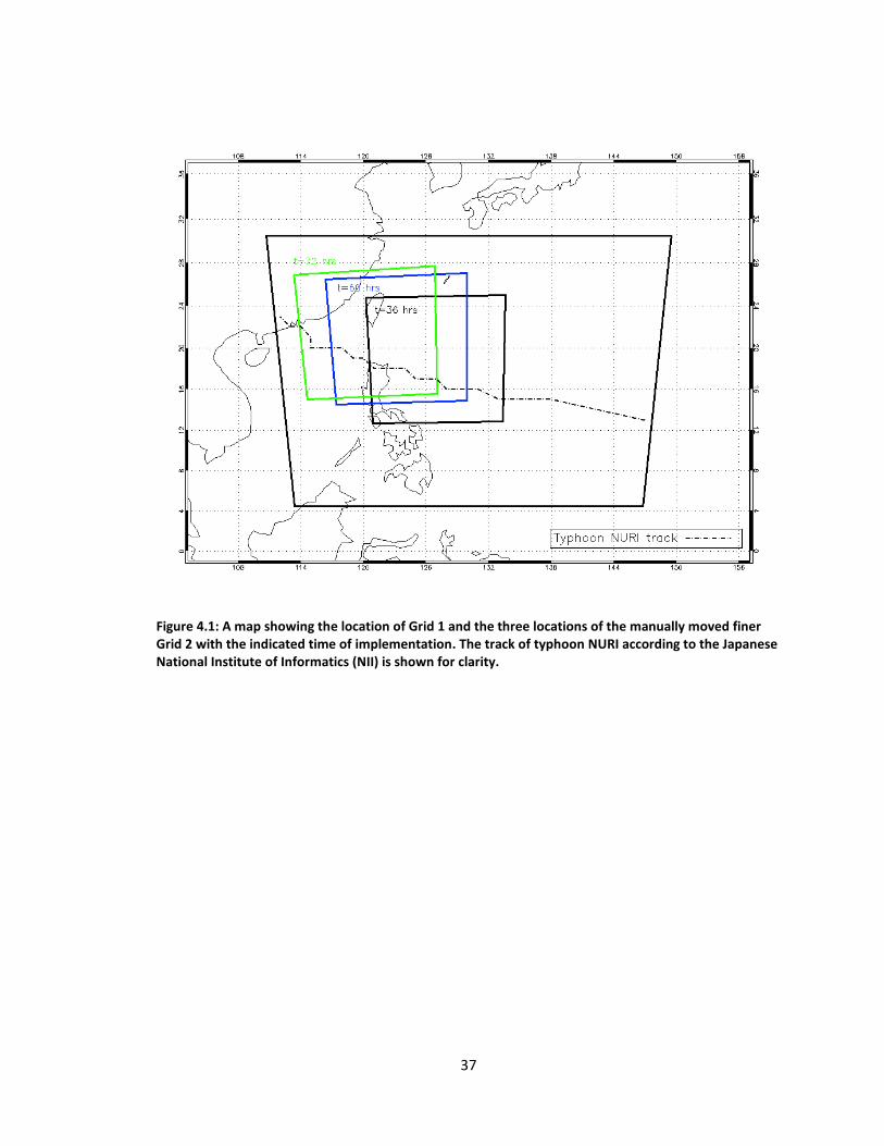
In order to capture the entire lifespan of the TC from cyclogenesis to landfall the second grid

had to be moved in order to keep the TC within its domain. Furthermore, the study's hypothesis

was contingent upon resolving the middle and outer rainbands of the storm, where the

additional CCN is expected to cause changes in cold-pool parameters. For this reason, Grid 2 was

manually moved twice throughout the simulation. This is a similar approach to explicitly

resolving convection and microphysical effects at cloud scale used by van den Heever et al.

(2006) simulating convective sea-breeze storms. The first move occurred at 60 hours from the

initial time of the simulation (24 hours after it was imposed). The grid was moved 375 km west

and 225 km north. The second move occurred at 72 hours since simulation start (12 hours after

the first move) and was moved another 300 km west and 75 km further north. The location of

Grid 1 and the three positions of Grid 2 are shown in Figure 4.1. This allowed the convection to

be explicitly resolved within the northwest rainbands of the TC. The entire simulation consisted

of 96 hours, beginning on August 17, 2008, 00 GMT and finishing on August 21, 00 GMT.

Convection was parameterized on Grid 1 using a Kain-Fritsch (Kain 2004) cumulus

parameterization scheme, but explicitly resolved for the finer grids. The time step for the larger

grid was 30 seconds and 15 seconds for the smaller grid.

4.2. Model Initialization

The model initialization was constructed via the Barnes scheme, as discussed in Chapter 2, with

both gridded and irregularly spaced point data. The gridded data utilized was the NCEP/NCAR

Renalysis 1 global gridded data (Kalnay et al. 1996). The data are updated every six hours and

have a horizontal resolution of 1.5 degrees and a vertical resolution involving 28 sigma levels

31

from the surface to 1 hPa. The horizontal and vertical components of wind, relative humidity

and geopotential heights are processed via the RAMS ISAN routine. The point data were

assimilated from the T-PARC dropsondes and incorporated into the gridded data as initialization

conditions and nudging files. The internal nudging of the model occurred 900 seconds during the

first 36 hours after which point, the internal nudging was switched off and only the boundary

conditions were nudged every 450 seconds.

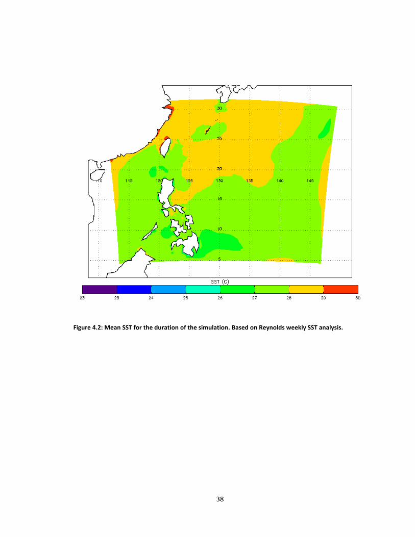
Reynolds weekly SSTs (Reynolds and Marsico 1993; Reynolds and Smith 1994) were used and

not updated during the simulation (Figure 4.2). Reynolds weekly SST analysis has a one-degree

resolution. The surface processes were parameterized using the Land Ecosystem-Atmosphere

Feedback (LEAF-2; Walko et al. 2000). The Harrington (1997) parameterization was used for

long/shortwave radiation and updated every 15 minutes and the Klemp and Wilhelmson (1978)

boundary conditions were applied at the lateral boundaries.

4.3. Aerosol Prescription

TC NURI was chosen in part due to its path which took it near centers of large aerosol activity. As

shown in Figure 4.3, the AOD in and near the TC path is significantly higher than the cleaner

maritime environment in which the TC was birthed. Geography and geometry of the trend of

AOD was taken into account when constructing this experiment. The MODerate Resolution

Imaging Spectroradiometer (MODIS) retrievals show the aerosol concentration at elevated

levels along the coast of China and extending to the northeast beneath the Japan. The elevated

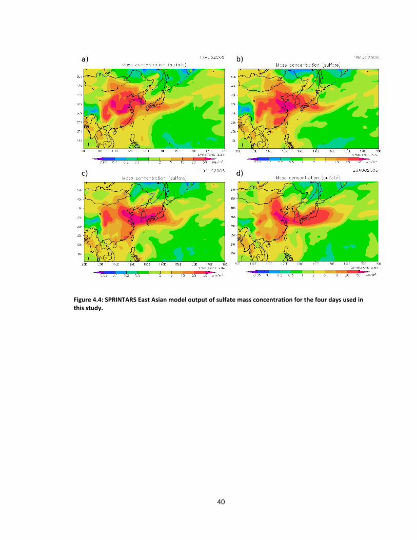
aerosol region provided by MODIS is further confirmed by the SPRINTARS three-dimensional

aerosol model (Takemura et al. 2000) data for the dates of the TC which show aerosol plumes of

sulfate (Figure 4.4) and dust (Figure 4.5) emanating from the Chinese and Indian coasts

32

advecting into the path of the TC. Both the MODIS satellite AOD retrievals and the SPRINTARS

horizontal and vertical aerosol model data data gave rise to the aerosol prescription used for

this study. The CCN prescription in the simulation follows the same middle to northeastern path

through the model domain and is regenerated every six hours as sources of CCN to represent

the continual influx of aerosol from the urban centers and the Gobi desert. As a result, the

northwest rainbands of the simulated TC entered the regions of elevated concentrations of CCN

first.

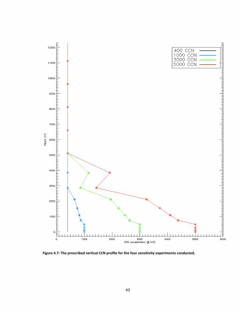
The vertical concentration of CCN was also constructed based on the SPRINTARS model.

SPRINTARS calculates the transport of aerosols taking into account emission, advection,

diffusion, wet deposition, dry deposition, and gravitational settling. The column aerosol

concentration for Beijing for the duration of the lifespan of TC NURI is shown in Figure 4.6. There

is a trend over the course of the TC lifespan of significantly elevated aerosol concentration of all

species from the surface to 3000 meters. There is also a smaller, second local maximum of

aerosol concentrations occurring near an elevation of 4000 meters. For the control simulation, a

homogeneous field of 100 CCN per cubic cm was applied and replenished every six hours in the

MODIS indicated domain. We use the Beijing SPRINTARS data (Fig. 4.6) as a guide to develop a

vertical profile of CCN, assuming a positive correlation between aerosol mass and CCN number

concentration. The vertical CCN prescriptions for the sensitivity studies are shown in Figure 4.7

and applied at each grid space within the geometric domain indicated by MODIS retrievals of

elevated aerosol concentrations. The naming conventions used for the remainder of this text

identifying each simulation are listed in Table 4.2.

33

Ice Nuclei and Giant CCN (GCCN) were not varied in this experiment and applied three-

dimensionally homogeneously at low, background concentrations. Table 4.1 summarizes the

model configuration and options for the TC NURI simulations.

4.4: Discussion of Control Simulation Results

This section will briefly introduce some of the results from the control simulation, or C100.

Further discussion appears in Chapter 5, including comparisons with the sensitivity tests.

RAMS was able to produce a TC under low CCN concentrations. Despite not being an idealized

simulation the vorticity yielded by the control simulation (Figure 4.8) is consistent with the

described results of Montgomery et al. (2006). As indicated by Figure 4.8, the TC NURI has a

westward tilt, consistent with the large scale meteorology of this case study and TCs in general.

We also note the weak upper-level vorticity (Fig. 4.8d) as TC NURI was formed in an unusually

high amount of shear (Raymond and Carillo 2010).

Grid-averaged maximum windspeed peaked at 54 hours into the simulation at about 30 m/s

sustained winds, consistent with observations from the T-PARC dropsondes and ECMWF

reanalysis data. The manually moved grid allowed for continued higher resolution in the

northwest quadrant of the storm (see Figure 4.9), although this technique did yield a few

modeling artifacts that must be considered. For instance, the rain rate was relatively constant

throughout the storm except at the time where the nested grid was moved manually, at 60 and

72 hours. Figure 4.10 shows the rain rate dropping off to zero at both times. As the nested grid

was moved, it took a brief amount of time for the nested grid to explicitly resolve convection

34

again. Still, explicit convection was achieved including a broad spectrum of hydrometeor

species, similar to a real TC. Chapter 5 will further analyze the achieved results of the control run

and the sensitivity tests.

35

4.5: Chapter 4 Tables and Figures

Table 4.1. RAMS model configuration and options.

Model Aspect Setting

Grid

Arakawa C grid (Mesinger and Arakawa 1976)

Two grids

Grid 1: ∆x=∆y =15 km; 253 x 200

Grid 2: ∆x=∆y=5 km; 452 x 452

Manual moving of Grid 2, follows TC path

Vertical grid: ∆z stretches from 120 m to 1500 m; 20 vertical levels

Initialization

Barnes objective analysis

NCAR/NCEP Reanalysis Data

T-PARC Dropsondes

Time Step Grid 1: 30 s; Grid 2: 15 s

Simulation duration

96 hours

08/17/2008 to 08/21/2008

Microphysics scheme

Two-moment bin emulating microphysics (Meyers et al. 1997; Feingold et al. 1998; Saleeby and Cotton 2004)

Convective initiation

Kain-Fritsch parameterization (Kain 2004) for Grid 1; explicit convection on Grid 2

Radiation scheme

Harrington (1997)

Sea Surface Temperatures

Reynolds weekly SSTs (Reynolds and Smith 1994; Figure 4.2)

Aerosol Prescription

Horizontal domain based on MODIS AOD retrievals (Figure 4.3)

Varying vertical CCN profile (Figure 4.7) for sensitivity tests based on SPRINTARS (Figure 4.4) model output

Regenerated every 6 hours

36

Table 4.2: Naming convention used for this study of each sensitivity test simulation of TC NURI

as well as the control run.

Simulation Identifier CCN concentration of elevated aerosol field (per cubic centimeter)

C100 or “Control” 100

C400 or “Moderately clean” 400

C1000 or “Moderately polluted”

1000

C3000 or “High” 3000

C5000 or “Extreme” 5000

37

Figure 4.1: A map showing the location of Grid 1 and the three locations of the manually moved finer Grid 2 with the indicated time of implementation. The track of typhoon NURI according to the Japanese National Institute of Informatics (NII) is shown for clarity.

38

Figure 4.2: Mean SST for the duration of the simulation. Based on Reynolds weekly SST analysis.

39

Figure 4.3: The AOD retrieved from MODIS averaged over the lifespan of TC NURI.

40

Figure 4.4: SPRINTARS East Asian model output of sulfate mass concentration for the four days used in this study.

41

Figure 4.5: As Figure 4.3, but for dust mass concentration.

42

Figure 4.6: SPRINTARS model output of column aerosol over Beijing for the dates of the study averaged by day.

43

Figure 4.7: The prescribed vertical CCN profile for the four sensitivity experiments conducted.

44

Figure 4.8: The relative vorticity of the C100 simulation at t=68 hours at the following vertical levels: a) 320m, b) 900m, c) 1800m, and d) 9000m.

45

Figure 4.9: Entire nested grid domain showing near-surface windspeed (m/s) and wind vectors for C100 simulation at t=52 hrs.

46

Figure 4.10: The rain mixing ratio within the downdrafts by height, along with the maximum rain rate. Note the precipitous drop in maximum rain rate at t=60 and t=72 hours. This is an artifact of the manually moving grid. However, the rain rate quickly became reinvigorated.

47

Chapter 5 CHAPTER 5 – RESULTS

5.1: General Discussion

The RAMS model was able to successfully reproduce a WP storm of TC strength under all CCN

experiments. The vortex as described in Montgomery et al. (2006) was implemented 36 hours

into the simulations. From there, the typhoon developed into a strong Category 1 / weak

Category 2 TC according to the Saffir-Simpson Hurricane Scale, exhibiting sustained winds

topping 30 m/s, consistent with the observations yielded by the T-PARC dropsondes and the

ECMWF Reanalysis data. The TC intensified similarly under all CCN experiments as the elevated

CCN concentrations were constrained closer to the Chinese coastline, as indicated by MODIS

retrievals and SPRINTARS model output. As such, the TC in each experiment intensified

identically from 36 hours to 48 hours (Figure 5.1) according to maximum windspeed. The

internal nudging of the model had been switched off at this point in the experiment. Therefore

any future response of the TC can be attributed to the CCN differentiation.

The outer rainbands of the TC began to ingest the elevated levels of CCN around the 46 to 50

hour mark. At the same time the TC continued moving in a northwestern direction, ostensibly

48

advecting itself over the ingested and produced CCN (see Chapter 4 for description of CCN

production). The TCs exhibit wildly different maximum windspeeds in the moderate CCN cases

(C1000 and C3000 experiments) upon the ingestion of CCN into the TC rainbands. In particular

the pattern of intensification from 56 to 64 hours differs under moderate CCN (C1000

experiment) and higher CCN (C3000) experiments. In C1000 the additional CCN produces a quick

increase in maximum windspeed while the C3000 produces a similar peak, but about 6 hours

later in the simulation. In both cases, the near 60-hour windspeed maxima far exceeds the clean

(C400) and extreme (C5000) CCN experiments. The underlying reasons for these responses will

be discussed later in this chapter.

Upon passing the near 60-hour maxima, the TC begins to dissipate somewhat into a tropical

storm with maximum sustained winds between about 20 and 25 m/s. As the TC passes the

Philippine coast and begins to cross slightly colder SSTs along the coastline, the storm maintains

the northwest track and stabilizes as a TS until it makes landfall on the Chinese coast. However,

in the C1000 there are two further peaks of sustained maximum windspeed at 74 and 82 hours

that would reclassify the storm as a Category 1 TC. Even again as the storm is dissipating at the

88 hour mark the C1000 case again exhibits a slight peak while the other TC experiments

continue to deintensify. As will be discussed in this chapter, the continual replenishment of CCN

in these experiments has the effect of creating and recreating convective activity that acts to

produce higher windspeeds due to downdrafts and cold-pool propagation than when CCN is

kept at a minimum. While not producing the periodic convectively generated maximum

windspeed peaks that the C1000 case does, the C3000 TC exhibits a general tendency to be a

few meters per second stronger than the C400 case (Figure 5.2) throughout much of the storms

49

lifespan. Interestingly, the two most similar experiments are the clean, C400, and the extremely

polluted, C5000, experiments, with the C5000 experiment showing a slight tendency to be

damped between 1 and 3 m/s from experiment hours 76 onward.

The TC tracks for each experiment, along with the best track given by the Japanese National

Institute of Informatics (NII) and the track of minimum geopotential height according to ECMWF

model data are shown in Figure 5.3. RAMS produces a storm that maintains a track error of

about 1.5 degrees rather consistently throughout the simulations. The model error yielded in

RAMS was similar to that of the forecasted track of the storm (Miyoshi et al. 2010). While the

C5000 exhibits the highest amount of drift in the TC track, the amount it differs in track is

negligible. In the dissipation phase of the storm the RAMS simulated track, the center of the TC,

as indicated by minimum perturbation pressure, turns southward bringing it more in line with

the NII and ECMWF indicated tracks.

5.2: Precipitation Modulation and Convective Activity

Additional CCN has been shown to alter precipitation in continental convective storms (van den

Heever et al. 2006, Seifert and Beheng 2006, Storer et al. 2010). This largely occurs due to an

alteration of the latent heat release resulting from the perturbation of the amount, location,

and timing of the freezing of cloud drops. As the CCN increases, the droplet concentration

increases and the size of droplets decrease. This results in less sedimentation, fallout, reduced

collision efficiency, and scavenging for the smaller droplets, as well as the tendency for the

droplets to freeze at lower sub-zero temperatures. The TC NURI experiments confirm there is

also a precipitation modulation due to additional CCN in the case of TCs. Figure 5.4 shows the

50

modeled reflectivity 74 hours into the simulation, or about 14 hours after initial contact with the

elevated CCN field. By this time the TC has advected over the location of initial CCN ingestion, as

indicated by the surface perturbation pressure contours. The convective activity takes on a

different form in terms of strength and distribution for each of the modeled experiments. At this

time C3000 shows the most vigorous convective activity at the southwest corner of the TC

center, while both the C1000 and C3000 show a significant secondary convective mode along

the northwest corner of the TC center. When comparing to the C400 case, we note that this

secondary convective mode is either absent or broken up into less vigorous convective cells. The

C5000 shows significantly damped convective activity at both convective locations. Similarly the

rain rate at this time (Figure 5.5) is greatly increased for C1000 and C3000 and significantly

damped for C5000. In all cases at this time, the locations of higher rain rates are located within

the elevated CCN field. Six hours later, C5000 does begin to show convective activity (Figure

5.6). Spatially, however, the reflectivity shows a distinct contour around the TC center. Also, it is

worth noting the high reflectivity over the Philippine Islands in the C5000, absent in the other

three cases. The additional CCN appears to have “locked in” some of the atmospheric

condensate until a time in which it may be condensed and precipitated out.

Due to the smaller droplet size, the condensed water is more susceptible to updrafts and

transported into the upper atmosphere. This is evident in Figure 5.7, which shows the average

condensate mass within the updrafts from the time of initial CCN ingestion (t=60 hrs). The

amount of condensate being uplifted away from the mid-troposphere in the C5000 case dwarfs

the other three experiments; twice as much condensate mass over the course of the model run.

Conversely, the opposite CCN-moisture flux association is true when we examine the

51

condensate in the downdrafts of the model runs. Figure 5.8 shows the average rain mixing ratio

within the downdrafts of the storm. In this instance, the C5000 case shows an enhanced rain

mixing ratio within the downdrafts below 1500 meters. Between 1500 meters and 4000 meters,

the C5000 case shows lower rain mixing ratios, evidence of a drier mid-troposphere, when

considered along with the condensate within the updrafts above 6000 meters (Fig. 5.7). The

convective trend continues at 86 hours into the simulations (Figure 5.9), with enhanced

modeled reflectivity in the C3000 case and almost none in the C5000 simulation.

Regarding the modulation of latent heat release, we now examine the presence of supercooled

liquid water (SCLW) for all simulations; that is, the mass of moisture above freezing level still in

liquid form. The time evolution of the amount of SCLW within the outer domain of the TC, as

defined as 250 km from TC center, is shown in Figure 5.10. The low to high CCN concentration

simulations (C400, C1000, and C3000) all show a time delay of maxima of SCLW compared to the

C100 case. These simulations reach their maxima two hours later than in the control run. The

C3000 simulation shows the greatest increase in SCLW, exceeding the control simulation by

1000 kg (or, 212%). This is by far the greatest amplitude change, however, each simulation

shows a distinct variance in peak SCLW, with the most polluted case, C5000, showing the latest

peak in SCLW.

When we examine the time-averaged amount of SCLW according to height (Figure 5.11) over

the course of the simulations we see a monotonic increase in SCLW just above the freezing level

except for the C5000 case, which shows a steep decrease in SCLW. The potential causes for

C5000’s decrease will be discussed later in this chapter. As for the other cases, the C3000 shows

52

a ubiquitous increase in SCLW at all height levels. C1000 shows an increase in SCLW compared

with C100 just above freezing level, a slight decrease in the mid-troposphere (around 9000

meters), and reverses trend again with C100, containing a higher SCLW at 10500 meters). By

altering the profile of SCLW, it stands to reason the profile of latent heat release would show a

similar alteration with increased CCN. In the next section, the impact of the variances in

hydrometeor activity will be examined alongside convective fluxes.

5.3: Downward Flux

Downward flux (DFX) is defined in (Riemer et al. 2009. Eq. 23) as

, (Eq. 5.1)

where ’ is the deviation of equivalent potential temperature from the azimuthal mean and

is the vertical velocity. This parameter yields an indication as to both the upward and downward

motion and the thermodynamics of the air being transported vertically. Essentially, in a period

of high convection and precipitation, the net downward flux will be strongly positive due to the

downdrafts and air associated with the downdrafts. Conversely, the DFX parameter will also be

positive for a strong upward flux of relatively high air. As suggested in Riemer et al. (2009),

DFX is calculated for the model height corresponding to about 1500 m to best represent the

inflow from the BL. The closest model height available for this study was 1300 m, so all DFX

calculations occur at that level. The time evolution of net DFX throughout the simulation is

shown in Figure 5.12. Here we see a pattern similar to some of the maximum windspeed

patterns (Fig. 5.1): invigorated DFX followed by a reduction in DFX. All simulations generally

follow the same trend of DFX: each local maximum is generally located at the same model hour

(t=68, 78hours) All sensitivity tests show an initial damping of positive DFX compared to the

53

control simulation until 68 hours. At this point all simulations except C5000 quickly show an

amplified DFX. The C3000 simulation shows a dramatic increase in DFX at this point in the

simulation, jumping to nearly 10000 K m/s. The C3000 case also shows a reinvigoration of DFX

six hours later that is absent in the other simulations. Cold-pool activity has been linked to

invigoration of MCSs; it is possible the abnormally strong cold-pool generated in the C3000

simulation had the effect of invigorating further convection. It is critical to remember too that a

strong positive DFX signal could either be indicative of strong downward flux of low or strong

upward flux of high . Once the second DFX maxima is reached, for the rest of the simulation

the C3000 case remains one of the more damped cases of DFX.

Once again, the C5000 base shows the most damped DFX, consistent with the reduced

convection described in the previous section. We also note that the C5000 case deviates

comparatively little in magnitude with the C100 case after the 60 hour mark: the DFX minima

and maxima are not as strong as in the other cases, generally staying within 2000 to 4000 K m/s.

One of the primary hypotheses of this study is that the imposition of higher CCN concentrations

will cause a variance in SCLW aloft, resulting in differences in convective and cold-pool activity in

a TC. The link between SCLW and convective activity can readily be seen in Figure 5.13. Here the

amount of SCLW is lag-correlated with DFX by two hours, with the linear correlation coefficients

(r) also shown. The strong r values for the C400, C1000, and C3000 indicate a linear relationship

between a high presence of SCLW and the DFX of a system two hours later. The composite r

value for all five simulations is 0.57. And if we exclude the extremely polluted case, where the

advection of SCLW away from the system is more of a factor (discussed in detail in section 5.5),

54

the correlation coefficient is 0.63: a clear sign of positive linear correlation. The generation of

large amounts of SCLW results in an eventual generation of large amounts of DFX.

We now examine the time evolution of DFX regionally compared to the TC center (Figure 5.14).

As we are largely concerned with the activity of precipitation within the outer rainbands, we

observe that the DFX response is stronger in the C1000 and C3000 cases when looking past 60

hours and 50 to 150 km from TC center. In the C1000 simulation starting at 78 hours, we can

evidently see the movement of strong DFX towards the center of the TC, an artifact of the

movement of the TC. A similar inward-tendency of strong DFX is evident in the C3000

simulation; however, as the additional CCN damps the DFX initially, the strongest period of DFX

is stronger and closer to the TC center. The C5000 simulation shows the most neutral DFX

response over the entire simulation. The maximum tangential windspeed is concurrently shown

in Figure 5.14, exhibiting a fluctuating response akin to the DFX strength.

The spatial distribution of DFX relative to TC center along with the wind vectors, indicating the

direction of the inflow of DFX in the BL are shown for the C100 and C3000 cases at 76 hours in

Figure 5.15. When examining the individual wind vectors, we note that the wind vectors

propagating from regions near strong DFX are pointed more outward than tangential to the TC

center. These wind vectors are pointed out in Figure 5.15. Even without considering CCN

concentration, we see a clear linkage between enhanced positive DFX and a disruption in the

storm dynamics from the strong downdrafts. In the C3000 case the region of strongest DFX is

closer to the TC center: 100 km west of the TC center for the C100 case, while only 50 km west

55

for the C3000 case. In this instance, it is possible the low air is more likely to be entrained in

the convective towers near the TC eye.

As discussed earlier, the C3000 case shows a strong reinvigoration of DFX near the 80 hour

mark, shown spatially along with the C100 case in Figure 5.16. Here the region of DFX is more

widespread. However, there are also pockets of negative DFX within the inflow layer. Recall

from the definition of DFX (Eq. 5.1), a region of negative DFX could be indicative of either an

upward flux of low air and/or a downward flux of high air. Another possibility is that this is

an artifact of the azimuthal averaging when calculating ’ as given in the definition. Adjacent to

extremely low , the pockets of negative DFX could simply be more damped regions

comparatively, but not necessarily exhibiting overly high or low raw values. Regardless, the

increase in both positive and negative DFX is indicative of strong convective activity at the BL

inflow layer. Rain mixing ratio within the downdrafts may also be examined over time and

according to height to obtain a better working knowledge of the convective activity of the

storm. As shown in Figure 5.17, the downdraft rain mixing ratios are altered according to the

CCN concentration field. From 64 hours to 74 hours, the simulations differ in terms of the rain

mixing ratio and how it is distributed vertically. The enhanced CCN cases all show levels of

enhanced downdraft rain mixing ratio existing higher in the atmosphere than in the cleanest

case. The clean, C400 case shows a maxima of downdraft rain mixing ratio at 68 hours,

extending no higher than 1500m above the surface. The C1000 delays that maxima by a few

hours and extends it vertically to nearly 3000m. The C3000 and C5000 each show two local

maxima of downdraft rain mixing ratio at 66 and 70 hours, which are also concurrent with

periods of maximum rain rate. Again, the extent of the relative maxima extends vertically to

2500m, suggesting a lifting of the level of precipitation compared to the C1000 case. In the next

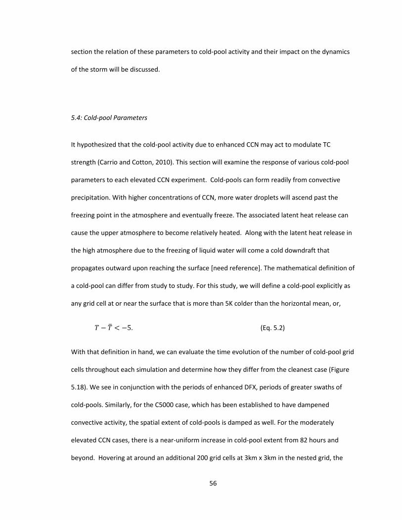
56

section the relation of these parameters to cold-pool activity and their impact on the dynamics

of the storm will be discussed.

5.4: Cold-pool Parameters

It hypothesized that the cold-pool activity due to enhanced CCN may act to modulate TC

strength (Carrio and Cotton, 2010). This section will examine the response of various cold-pool

parameters to each elevated CCN experiment. Cold-pools can form readily from convective

precipitation. With higher concentrations of CCN, more water droplets will ascend past the

freezing point in the atmosphere and eventually freeze. The associated latent heat release can

cause the upper atmosphere to become relatively heated. Along with the latent heat release in

the high atmosphere due to the freezing of liquid water will come a cold downdraft that

propagates outward upon reaching the surface [need reference]. The mathematical definition of

a cold-pool can differ from study to study. For this study, we will define a cold-pool explicitly as

any grid cell at or near the surface that is more than 5K colder than the horizontal mean, or,

. (Eq. 5.2)

With that definition in hand, we can evaluate the time evolution of the number of cold-pool grid

cells throughout each simulation and determine how they differ from the cleanest case (Figure

5.18). We see in conjunction with the periods of enhanced DFX, periods of greater swaths of

cold-pools. Similarly, for the C5000 case, which has been established to have dampened

convective activity, the spatial extent of cold-pools is damped as well. For the moderately

elevated CCN cases, there is a near-uniform increase in cold-pool extent from 82 hours and

beyond. Hovering at around an additional 200 grid cells at 3km x 3km in the nested grid, the

57

moderately elevated CCN cases translate to a roughly 1800 square km increase at each time

step.

Upon analyzing the cold-pool activity, we must also take the location of the cold-pools into

account. Based on the mean meteorology of the WP, a TC will advect in a westward direction,

which acts to advect itself over locations of elevated anthropogenic aerosols. In this sense, it

differs from Atlantic TCs that interact with African dust from the SAL. In the case of the SAL, the

dust is transported into the outer rainbands of a TC from the rear, while this and other WP TCs

ingest aerosol, then drift over the location where aerosol was ingested. This results in a different

dynamical response and gives rise to a different set of working hypotheses.

In that context, buoyancy is examined. As defined in Emmanuel (1994), buoyancy is given as

(Eq. 5.3)

where is the acceleration due to gravity and is the density potential temperature,

(Eq. 5.4)

and is the potential temperature and and are the mixing ratios for vapor, cloud

condensate and rain, respectively.

As suggested in Tompkins (2001), buoyancy may act as a proxy for cold-pools. We compare the

evolution of a buoyancy-pool (Figure 5.19) for the C400 and C3000 cases, along with the

location of the TC center. Each frame is separated by two hours of model time. We note in both

58

cases how the storm center passes through the generated cold-pool, beginning at 76 hours. By

this time, roughly 16 hours have passed since the storm initially came into contact with the

elevated CCN field. At 74 hours, the shape of the cold pools differ in that the C400 shows a

radial patch of negative buoyancy while the C3000 shows a more “squall-like” cold pool, curving

around the center of the storm. At 76 hours, the storm has drifted over the cold pool. However,

the mid-to-outer extent of the TC differs in buoyancy. In the C400 cases there are two patches

of positive buoyancy, one just south of the TC center and the other about two degrees east of

the TC center, both of which are non-existent in the C3000 case. By this time the enhanced CCN

field has sufficiently wrapped around the storm (see Fig. 5.5), so the additional CCN has caused a

much greater extent in negatively buoyant air throughout the TC’s storm outer band region.

There is even a small second cold pool at this time in the C3000 case, not present in the cleaner

case, east and slightly north of TC center. As at 74 hours, the C3000 cold-pool is non-uniform in

shape and scope.

In fact, the non-uniformity of the cold pool can be observed when we examine the relative

vorticity at an elevation 1300m (Figure 5.20). While in the C400 case we observe organized

bands of generally positive relative vorticity, in the C3000 case we see tiny patches of negative

vorticity. These patches are assumed to be caused by small eddies emanating from the

negatively buoyant cold-pools occurring at the same time at the surface (Fig. 5.19). In theory,

this could act to break up the storm, however, it is not evident when we compare the response

to the overall maximum windspeed (Fig. 5.2).

In the other elevated CCN cases (C1000, C5000; Figure 5.21) we see a similar absence of positive

buoyancy that we observed in the C400 case (Fig. 5.19c). We also see a similar lack of uniformity

59

in cold-pool shape. The C5000 case for instance shows an enclosed region of less negatively

buoyant air just near the TC center (Fig. 5.21e).

The buoyancy parameter, which is a function of , effectively measures the tendency of air to

be able to ascend or descend at a given point. The cold-pools have been shown to penetrate the

inner core of the storm. If we examine the equivalent potential temperature directly, we can see

the potential additional aerosol may have to disrupt the storm. Figure 5.22 shows the azimuthal

average around the storm of at 84 hours into the simulations. In the clean, C400 case, we see

a classic example of a warm-core TC with regions of high near storm-center. In the enhanced

CCN cases we see a suppression of the convectively generated “hot towers” with lower air

near the storm-center at or above 1500m. Moreover, the C1000 and C3000 show a tendency for

low air to dip to near-BL levels and impinge into the middle of the TC. The C5000 case, with

its damped convection, shows a much more horizontal gradient of indicating limited

downdraft and convective fluxes.

Two hours later (Figure 5.23) we see the TC in one of its convectively active periods, as indicated

by the prevalence of influx of low air. This time, the C1000 case shows a near complete

suppression of the convective “hot towers” near the center of the storm. The downdrafts

present are strongest near the TC center at this point in the C1000 case. The C3000 case shows

the existence of another patch of low 170 km away from TC-center, potentially ready to

advect into the center of the storm.

60

5.5: Response of Hydrometeors

The imposition of elevated aerosol concentrations has been theorized and simulated to affect

the number concentration, size, and type of hydrometeors in the atmosphere. As discussed in

Chapter 2, the RAMS model allows for eight classes of hydrometeors. For this section, we will

focus on five: cloud droplets, rain droplets, pristine ice, snow, and aggregates. Hail and graupel

were excluded from the hydrometeor plots for clarity. Examining the aerosol impact on

hydrometeors will aid in the explanation of the varying convective activity throughout the life of

the TC.

A cross section of the storm at 64 hours showing the different mixing ratios for the five

hydrometeors in question, plotted in Figure 5.24, for the C400 and C3000 case is instructive as

to the significant effect of additional CCN on convective fluxes and precipitation regimes. The

C400 case at this time exhibits strong precipitation, as indicated by the elevated rain mixing

ratio to the west of the storm reaching the surface while the C3000 shows reduced rain mixing

ratio. There is however, the presence of an elevated pristine ice mixing ratio above 10000m. In

this case, much of the condensate has remained in the atmosphere as a result of the additional

CCN’s ability to initially suppress rainfall. Figure 5.25 shows the same information 6 hours later.

Here, we see the C3000 is now the storm with heaviest precipitation. Also at this time we note

the heaviest precipitation is east of the storm. The cloud mixing ratio appears to be of similar

concentration and vertical distribution while the snow and aggregates mixing ratios are more

substantial in the cleaner case. At both times, the C400 case has a more uniform distribution of

all five hydrometeor types suggesting a more balanced distribution of hydrometeor species,

more akin to the control simulation. Meanwhile the more polluted cases appear to favor the

61

production of pristine ice while suppressing snow. The additional pristine ice provided by the

additional CCN can then be advected away from the storm at high elevation, failing to

precipitate back to the surface. This is evident when examining the extreme case of high CCN

(the C5000 case; Figure 5.26). Here we see even the C3000 case precipitating substantially and

transitioning from ice to snow at about 10000m, then finally as cloud and rain mixing ratios

below 5000m. For the C5000 case, now at 68 hours into the simulation, all these five

hydrometeor species are present, but in differing mixing ratio concentration. Here, the vertical

distribution of ice in the C5000 case stretches well past 15000m while the C3000 case appears

capped. The mixing ratio of aggregates is substantially higher in the C5000 case. Presumably the

size of the cloud droplets in the less polluted case are larger and are less subject to updrafts as

well as being easier to fall out by precipitation, sedimentation, or scavenging. Much of the

moisture is in the form of aggregates at this time in the C5000 case.

This size difference of hydrometeors under different CCN concentrations is evidence of indirect

effects of aerosol ingestion into clouds. As the atmosphere ingests more and more CCN similar

amounts of condensed water will result in smaller nucleated droplets. As these droplets are

caught in updrafts, the smaller particles will be thrust further up in the atmosphere until they

are carried away by the inevitable divergence of the wind, presuming the particles are small

enough and the updrafts are vigorous enough.

As we look at the time evolution of droplet number for all four sensitivity tests we can readily

see the indirect effects of increased aerosol concentration on number concentration of the five

hydrometeor species. At 62 hours (Figure 5.27) the outer rainbands have just come into contact

62

with the elevated CCN field. Immediately, we see a near monotonic decrease in snow (a

moderately rimed ice species in RAMS) and an increase in the number concentration pristine

ice, particularly in the two more extreme pollution regimes. At this time, the C1000 and C3000

cases are the more highly precipitating regimes. Twelve hours later (Figure 5.28), the C3000 case

shows evidence of the pristine ice being carried away in the upper atmosphere, above 10000m

due to the diverging winds. This is also one of the more convectively active periods of the storm

and the C3000 exhibits high precipitation near the storm center while the other three cases

show increased rain concentration about 100 km away from the TC center. Again, we see the

suppression of snow distribution with increasing concentration of CCN. Six hours later, now at

80 hours into the simulation, and about 20 hours after the storm has come in contact with the

elevated aerosol levels, the C1000 and C3000 cases are very connectively active (Figure 5.29).

Interestingly in the C3000 case there are multiple columns of high rain number concentration

and an increased drizzle regime about 500 km away from storm center. The number

concentration of pristine ice stretches well above the freezing level at this point in the more

polluted cases, capping out well past 15000 meters above the surface. As at previous time steps,

the C5000 case appears to be vertically advecting condensate in the form of pristine ice aloft. As

this ice is lofted and advected away, it loses the ability to be re-entrained in the storm, removing

it as a potential source of energy to help maintain or intensify the storm. We see a similar

dynamic occurring 6 hours after that (Figure 5.30): the highly polluted C3000 case is producing

significant precipitation while the extremely polluted case is producing almost none. This

phenomenon suggests a point of maximum aerosol impact as far as convection goes. After a

certain CCN threshold, the additional CCN does not invigorate convective activity, but rather

condensate transport in the anvils is enhanced by reducing the riming of ice particles aloft. In

theory, both of these phenomena could act to weaken a TC. Invigorated convection in the outer

63

rainbands could potentially lead to enhanced cold-pool activity, cutting off the energetics of the

system with low air, or water substance could be removed directly by the vertical advection

away of tiny pristine ice crystals. Recall Figures 5.7 and 5.8, showing the removal of water

substance in the mid-troposphere in the C5000, and in particular the mass condensate

contained within the updrafts (Figure 5.8).

The hypothesis relating extreme concentrations of CCN and droplet size are confirmed in Figure

5.31. In the most highly polluted case the mean cloud droplet diameter is smaller throughout

the simulation. Being smaller, these droplets are less likely to fall out and will also have a lower

sub-zero freezing temperature. The remaining three CCN sensitivity tests’ time-distance

evolution of mean cloud droplet size mimics the aforementioned convective pattern of

invigoration and subsidence. It is worth noting that the cleanest case shows the most “medium-

sized” drops (between 9 and 18 microns in diameter) whereas the C1000 and C3000 cases have

more extreme mean droplet diameters, both large and small. For rain droplet size the

sensitivity tests show an increase in diameter during convective periods for increasing CCN,

excepting C5000 (Figure 5.32). With more vigorous convective updrafts, a droplet is able to grow

larger due to its longer residency within the cloud mass, despite the initially smaller size as a

cloud droplet. This also suggests more available moisture aloft, confirmed by the relatively high

presence of aggregates in the cross section diagrams (e.g. Fig. 5.29) for the C3000 simulation.

The effect of rain drop size on cold-pool area via evaporative cooling may also be extrapolated.

At 74 hours, the rain drop size of the C3000 is much higher than in the other simulations (Fig

5.32), however, the cold-pool area two hours later is smaller than that of the C400 and C1000

simulations (Fig. 5.19). This suggests another added layer of complexity to the system in which a

64

larger droplet size regime may result in less evaporative cooling at the surface, hindering cold-

pool development. Still, while the feedback is negative, it’s counterbalanced by an increase in

convection overall.

As discussed previously, the C3000 cold-pool shape is more “squall-like” (Figure 5.14). The

presence of these squalls could work to produce further convection as suggested by Simpson

(1980). This appears to be what is happening in Figure 5.25. The precipitation has generated a

cold-pool which is in turn generating other regions of convection. This is also hinted at in the

diagram of relative vorticity (Figure 5.15) showing tiny anti-cyclonic patches. It is worth noting

that at this time (86 hours) the gross maximum windspeeds of all the simulations are not

dissimilar (Figure 5.1). In fact, the C3000 case contains the strongest maximum windspeed,

presumably due to the convective activity. However, these cold-pool results are instructive and

point to the ability of additional CCN to modulate cold-pools (Carrio and Cotton 2010).In a

stronger TC, it is possible the windspeeds will not be increased by the convective activity itself,

but could be subject to additional convective fluxes and low air.

65

5.6: Chapter 5 Figures

Figure 5.1: The maximum sustained near surface windspeed for the control simulation and each of the sensitivity tests and the recorded maximum near surface windspeed from the T-PARC dropsondes.

66

Figure 5.2: Difference of near surface maximum windspeeds from the C100 case for each sensitivity tests.

67

Figure 5.3: The track of TC from each sensitivity test as determined by perturbation pressure and NII best track and ECMWF Reanalysis Data as given by geopotential height.

68

Figure 5.4: The surface modeled reflectivity (dbz) at t=74 hrs with perturbation pressure contours of 1 mb for each sensitivity test.

69

Figure 5.5: Rain rate (mm/hr) at t=74 hrs for each sensitivity test. Selected contours of CCN concentration are shown to demonstrate the entrainment of the CCN into the storm.

70

Figure 5.6: As Figure 5.4, but at t=80 hrs.

71

Figure 5.7: Average total condensate mass within updrafts of 1.0 m/s or greater from 60 to 96 hours according to height for each sensitivity test.

72

Figure 5.8: Average rain mixing ratio within downdrafts greater than -0.25 m/s from 60 to 96 hours according to height for each sensitivity test.

73

Figure 5.9: As Figure 5.4, but at t=86 hrs.

74

Figure 5.10: The total amount of SCLW (kg) within the TC domain by time for each simulation.

75

Figure 5.11: Grid cell average of SCLW mass (kg) by height over the course of each simulation.

76

Figure 5.12: Net DFX over the inner grid domain at 200m height at over the course of each simulation for control simulation and all sensitivity tests.

77

Figure 5.13: Scatterplot of SCLW and DFX (lagged two hours) for all simulations. Linear correlation coefficients (r) for each simulation are shown. The composite r value is 0.57.

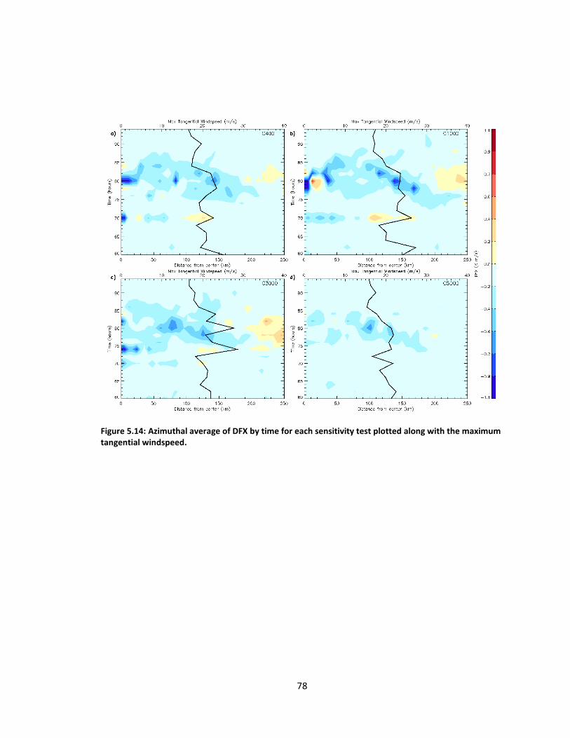
78

Figure 5.14: Azimuthal average of DFX by time for each sensitivity test plotted along with the maximum tangential windspeed.

79

Figure 5.15: DFX and wind vectors at t=76 hours for C100 (top) and C3000 (bottom) simulations. Circles indicated wind vectors that have been affected by propagating cold-pools.

80

Figure 5.16: As Figure 5.15 but for t=80 hours.

81

Figure 5.17: Average rain mixing ratio (g/kg) within downdrafts by time according to height. Maximum rain rate is plotted according to simulation time.

82

Figure 5.18: Change in the number of cold-pool grid cells (see text for definition) for nested grid from C100 simulation over time.

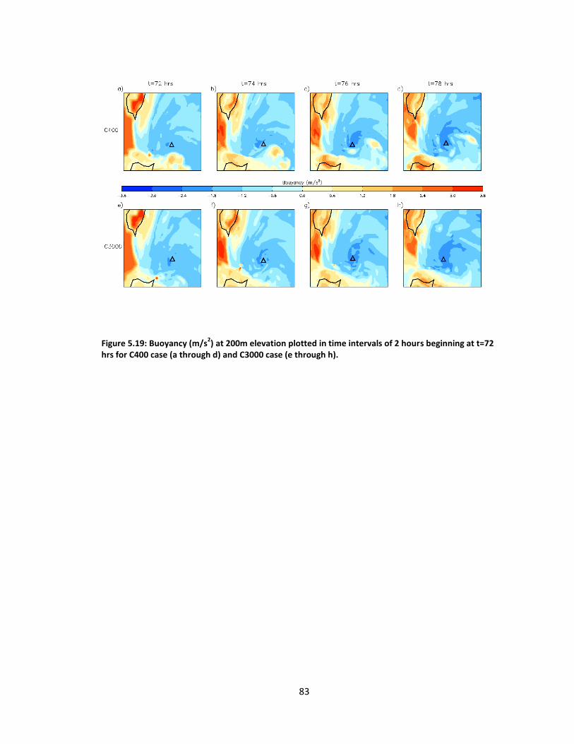
83

Figure 5.19: Buoyancy (m/s2) at 200m elevation plotted in time intervals of 2 hours beginning at t=72

hrs for C400 case (a through d) and C3000 case (e through h).

84

Figure 5.20: Relative vorticity at t=76 hrs and height 1300m for C400 and C3000 cases.

85

Figure 5.21: As Figure 5.14, but for C1000 (a through d) and C5000 (e through h) cases.

86

Figure 5.22: Azimuthal average of according to height at t=80 hrs. Azimuthal average of downdraft contours of -0.5 m/s are also plotted (dashed lines).

87

Figure 5.23: As Figure 5.17, but for t=84 hrs.

88

Figure 5.24: Cross section of storm at t=64 hrs showing mixing ratios for five selected hydrometeor species for C400 (a) and C3000 cases (b). Center of the TC according to minimum sea level pressure is also plotted (dashed line).

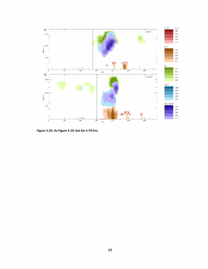
89

Figure 5.25: As Figure 5.19, but for t=70 hrs.

90

Figure 5.26: As Figure 5.19, but for C3000 (a) and C5000 (b) cases and t=68 hrs.

91

Figure 5.27: As Figure 5.19, but for number concentration of five selected hydrometeor species, all sensitivity tests (a: C400; b: C1000; c: C3000; d: C5000), at t=62 hrs. Cloud droplet concentration is in units of cm

-3; all others are in units of m

-3.

92

Figure 5.28: As Figure 5.22, but for t=74 hrs.

93

Figure 5.29: As Figure 5.22, but for t=80 hrs.

94

Figure 5.30: As Figure 5.22, but for t=86 hrs.

95

Figure 5.31: Azimuthally averaged cloud droplet diameter (microns) according to distance from TC center by time for all sensitivity tests (a: C400; b: C1000; c: C3000; d: C5000).

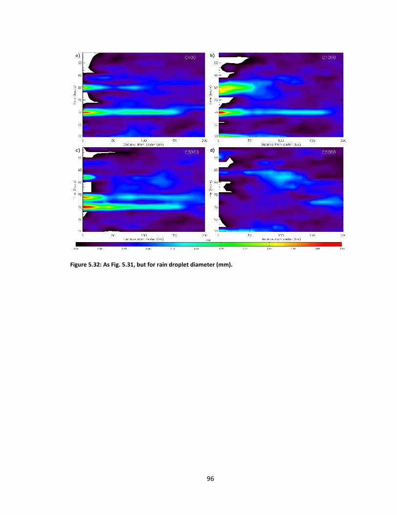
96

Figure 5.32: As Fig. 5.31, but for rain droplet diameter (mm).

97

Chapter 6 CHAPTER 6 – CONCLUSIONS

6.1: Summary of Study

The RAMS regional model with two-moment bin emulating microphysics was used to simulate a

2008 typhoon entering fields of elevated CCN concentrations. The model was initialized with

both gridded reanalysis data and irregularly spaced and timed dropsonde data obtained from

the T-PARC campaign. The CCN domain and vertical profile were derived from both MODIS

satellite retrievals and SPRINTARS aerosol model output. The simulations utilized a manually-

moved nested grid in order to best represent the microphysical activity beginning in the

northwest rainbands where the elevated CCN first became ingested into the storm. The

simulations ran for 96 hours with internal nudging switched off after 36 hours, allowing the

storm to develop from the model equations only. In all, five simulations differing only by CCN

concentration were run: a control run of 100 CCN per cubic centimeter applied homogeneously

over the model domainand four sensitivity tests of elevated CCN fields with concentrations of

400, 1000, 3000, and 5000 per cubic centimeter. The TC began to enter the elevated CCN fields

and ingest the CCN at the 56 hour mark.

98

6.2: TC Speed and Track

The maximum windspeeds and track of the simulated TC are consistent with the ECMWF

reanalysis and T-PARC dropsonde data after the internal nudging was switched off. After an

initial amplification of windspeed, the invigorated convection and other dynamical aspects

potentially resulting from the elevated CCN reduced the windspeed after the 74 hour mark (Fig.

5.2), with only brief periods of amplified windspeed. The most polluted case (C5000) showed the

most consistent damping of windspeed compared to the control simulation and all other

sensitivity tests. However, it is difficult to immediately assign additional CCN as a TC intensity

damping agent, without first considering its more direct links to changes in other parameters.

6.3: Droplet size, SCLW, and Convective Fluxes

The ingestion of increased CCN concentrations resulted in a smaller cloud droplet size (Fig 5.31),

particularly in the mid to outer rainbands of the TC (50 km to 100 km from TC center). Smaller

liquid droplets result in three immediate effects:

1. An initial reduction in precipitation. The cloud droplets are less likely to be coalesced or

scavenged in precipitating regimes. However, this does not imply an overall reduction in

precipitation. Due to other effects of the smaller droplet sizes, the convectively

produced precipitation can possibly be increased later in the storm, similar to the results

in Seifert and Beheng (2006).

2. The droplets will be more subject to updrafts. In addition to having a smaller mass and

being more susceptible to updrafts, the fall-speed of the smaller particles is reduced,

causing the system to retain more condensate at higher levels.

99

3. A lower sub-zero freezing level. The reduction in collision-coalesence processes brought

on by smaller hydrometeors reduces the possibility the moisture may be removed from

the system via precipitation, sedimentation or scavenging. This results in smaller

droplets existing at temperature levels closer to the temperature at which homogenous

freezing occurs (-40 C). Therefore the lifted mass of freezing water can alter the vertical

heating profile of a system due to the vertical perturbations in latent heat release.

These three immediate effects of the elevated CCN were evident in the sensitivity tests in the

form of more SCLW (Fig. 5.10). The increase in SCLW led to a direct increase in convectively-

produced downdrafts, as given by DFX. Net DFX lag-correlated strongly with SCLW (Fig. 5.13),

particularly in the moderate CCN simulations.

6.4: Cold-pool Modulation

The increase in convective activity resulted in appreciable cold-pool modulation. As defined by

raw temperature change (Eq. 5.2, Fig 5.18), buoyancy (Eq. 5.3, Figs. 5.19, 5.21), and (Figs.

5.22, 5.23), the cold-pool activity differed significantly under different CCN conditions. The

C3000 simulation in particular showed evidence of low air intruding into the inflow of the TC

(Figs. 5.22c, 5.23c). Interestingly, Reimer et al. (2009) showed a similar cold-pool response using

increasing shear instead of CCN. The shape of the cold-pools also differed under elevated CCN

levels. The C3000 case for example, developed a negative-buoyancy pool (Fig. 5.19) that was

more “squall-like” in shape which eventually drifted beneath the TC eye. While it is difficult to

directly attribute the cold-pool’s presence, strength, and domain to TC deintensification, the

100

addition of dry, cool air would act to disrupt the energy source of a TC requiring large amount of

moist, warm air, as proposed by Wang (2002).

6.5: Two Potential Routes of CCN to Weaken a Storm

While noting the difficulty in directly and explicitly linking additional CCN to TC deintensification,

this study provides two routes for this potential phenomenon.

1. Increased convective activity leading to a decrease a TC’s energy source: warm, moist

air. After the initial damping of precipitation, the moderately polluted simulations

(C1000 and C3000), showed a dramatic increase in the downward flux of low air.

Upon reaching the BL the low air swept out and eventually into the TC eye.

Presuming the “bottom-up” development of TCs (Montgomery and Enagonio, 1998;

Hendricks et al, 2004; Montgomery et al, 2006), an influx of cold-pool air could weaken

a storm or at least hinder a TC’s intensification.

2. The removal of moisture from the system in the form of pristine ice. The highest CCN

simulation (C5000) showed the least amount of convective downdrafts in the form of

net DFX (Fig. 5.12) and cold-pool area increase (Fig. 5.18). However, the system did

show a perturbation in windspeed compared with the control run. Upon noting the

smallest droplet size yielded by the C5000 simulation (Fig. 5.31d), we hypothesize that

the droplets are sufficiently small to be frozen or rimed heavily and advected away from

the system as pristine ice, rather than precipitating to the surface. Evidence of this rests

in the form of elevated mixing ratios of ice aloft exiting the storm center (e.g. Fig. 5.26b)

as well as the drying out of the mid-troposphere throughout the simulation through

vertical moisture advection (Figs. 5.7 and 5.8). It is worth noting that C3000 also showed

some evidence of the enhanced vertical transport and advection away of pristine ice

101

(Fig. 5.26b), yet was still able to produce sufficient convection and precipitation. This

result is consistent with Carrio and Cotton (2010) which showed a similar response

under extreme CCN conditions. This study and that of Cotton and Carrio (2010) suggest

a “tipping-point” of sorts where additional CCN will switch from a “convection-creating”

regime to a “moisture-removing” regime. A schematic diagram of the potential for

extreme amounts of CCN to suppress TC strength via ice advection aloft is shown in

Figure 6.1.

6.6: A Comment on the Importance of Microphysics in TC Forecasting and Predicting

The inclusion of advanced microphysics into TC forecast and prediction models could prove both

instructive and strategic. As evidenced by this study, varying only a single moisture nucleation

species (CCN) yielded significantly different dynamical results. Giant cloud condensation nuclei

(GCCN) and IN were not varied for this study, but could also potentially affect the dynamics of a

TC. However, it is difficult to conclusively prescribe aerosol concentration and species given the

lack of observational platforms. The sources of the aerosols in question complicate matters

further: the chemistry of anthropogenic Chinese aerosol is notoriously complex and at this point

there are still open questions as to the nature of the aerosols produced – are they hydroscopic,

hydrophobic, or neutral? How does the chemistry of the aerosol change throughout its lifetime?

Are the aerosols radiatively active? This study did not include the direct radiative effect of

aerosol.

Explicit resolution of convection and nucleation of CCN in the nested grid necessitates the use of

a fine grid on the scale of 3 to 7 km resolution. Initial simulations using 10 km grid spacing

102

damped the response of the additional CCN, particularly the convective fluxes. The inclusion of

microphysics into TC forecasting models and testing the results is an endeavor worth

undertaking. As computing power continues to increase, the meshing of advanced microphysics

into TC forecasting and predictions will become less expensive computationally. And as the

practice becomes more widespread, it will become easier to compare and evaluate the

microphysical schemes implemented. Still, while TC forecasting models lag behind mesoscale

models in resolution, it is unlikely that an advanced microphysics scheme will practically be able

to be implemented into real-time forecasts.

6.7: Recommendations for Future Work

As described in the previous section, the ability of aerosols to become active nucleation sites for

water or ice is still not well understood. Moreover, even the concentrations of the different

species of aerosols are not well known. While aerosol transport models improve, sampling and

observational campaigns of aerosols are still scant in their deployment. Any verification of a

model’s ability to well represent microphysical impacts on a TC would begin with better aerosol

data.

The resultant change of TC intensity yielded by this study is instructive, but not conclusive. Still,

the impact of CCN on SCLW and convective downdrafts is evident. Further cold-pool analyses

could prove insightful as this study noted a strong cold-pool signal on the TC dynamics. In

particular, the mapping of cold-pools, and the TC’s response to their strength, shape, size, and

timing would provide further evidence on the susceptibility of a TC to be affected at the BL

103

inflow region and perhaps the eventual damping of storm intensity. The addition of CCN is only

one potential route to cold-pool enhancement. Cold-pools may also be modulated by shear and

moisture content.

Coupled Ocean-Atmosphere mesoscale model simulations would provide an enhanced

understanding of the effect of CCN on incoming shortwave radiation and the potential for

cooling off the surface of the ocean, which could also modulate TC strength.

This study, as all TC-aerosol studies, is by no means comprehensive. The simulations conducted

were especially regime specific, consisting of a particular CCN domain, TC intensity,

meteorological background, aerosol species, etc., all of which could alter the impact of aerosols

on the development of a TC. These and other variables could be explored with different regional

and/or TC forecasting models. The “alpha-testing” of an advanced microphysics scheme into a

real-time TC forecasting model could provide the most immediate and significant test case

scenario of TC-aerosol interaction to date.

104

6.8: Chapter 6 Figures

Figure 6.1: A schematic showing the potential of extreme amounts of CCN to suppress TC strength via the removal of moisture from the system in the form of ice aloft. The additional CCN works to reduce hydrometeor size such that collision-coalescence and riming are greatly reduced. The ice crystals may then be advected away from the system due to their inability to precipitate back to the surface.

105

REFERENCES

Albrecht, Bruce A. “Aerosols, Cloud Microphysics, and Fractional Cloudiness.” Science 245.4923

(1989): 1227-1230.

Anderson, Suzanne P. et al. “Integrated hydrologic and hydrochemical observations of Hidden

Creek Lake jökulhlaups, Kennicott Glacier, Alaska.” J. Geophys. Res. 108.F1 (2003): 6003.

Arakawa, Akio, and Vivian R Lamb. “A Potential Enstrophy and Energy Conserving Scheme for

the Shallow Water Equations.” Monthly Weather Review 109.1 (1981): 18-36.

Bahreini, Roya et al. “Aircraft-based aerosol size and composition measurements during ACE-

Asia using an Aerodyne aerosol mass spectrometer.” J. Geophys. Res. 108.D23 (2003):

8645.

Barnes, S. L., 1973: Mesoscale objective analysis using weighted time-series observations. NOAA

Tech Memo. ERL NSSL-62, National Severe Storms Laboratory, Norman, OK 73069, 60

pp. [NTIS-COM-73-10781].

Bender, Morris A. et al. “Modeled Impact of Anthropogenic Warming on the Frequency of

Intense Atlantic Hurricanes.” Science 327.5964 (2010): 454-458.

Berglen, Tore F. et al. “A global model of the coupled sulfur/oxidant chemistry in the

troposphere: The sulfur cycle.” J. Geophys. Res. 109.D19 (2004): D19310.

Braun, Scott A, and Wei-Kuo Tao. “Sensitivity of High-Resolution Simulations of Hurricane Bob

(1991) to Planetary Boundary Layer Parameterizations.” Monthly Weather Review

128.12 (2000): 3941-3961.

Carmichael, Gregory R. et al. “Changing Trends in Sulfur Emissions in Asia:  Implications for Acid

Deposition, Air Pollution, and Climate.” Environmental Science & Technology 36.22

(2002): 4707-4713.

Carrio, G. G., Cotton, W. R., 2010: Investigations of aerosol impacts on hurricanes: Virtual

seeding flights. (In process of submission). Atmos Phys Chem.

106

---. 2010: Study of the feasibility of the mitigation of the intensity of tropical cyclones by CCN

seeding in the outer rainband region: A HAMP Project, 29th Conference on Hurricanes

and Tropical Meteorology.May 10-14, 2010, Tucson, AZ

Charlson, R. J. et al. “Climate Forcing by Anthropogenic Aerosols.” Science 255.5043 (1992): 423-

430.

Charney, J., Eliassen, A., 1964: On the growth of the hurricane depression. J. Atmos. Sci.,21, 68-

75.

Chen, Tsing-Chang et al. “Role of the Monsoon Gyre in the Interannual Variation of Tropical

Cyclone Formation over the Western North Pacific.” Weather and Forecasting 19.4

(2004): 776-785.

Chin, Mian et al. “A global aerosol model forecast for the ACE-Asia field experiment.” J. Geophys.

Res. 108.D23 (2003): 8654.

Clarke, A. et al. “Sea-Salt Size Distributions from Breaking Waves: Implications for Marine

Aerosol Production and Optical Extinction Measurements during SEAS*.” Journal of

Atmospheric and Oceanic Technology 20.10 (2003): 1362-1374.

Cotton, William R. “Numerical Simulation of Precipitation Development in Supercooled Cumuli—

Part I.” Monthly Weather Review 100.11 (1972): 757-763.

---. “Numerical Simulation of Precipitation Development in Supercooled Cumuli—Part II.”

Monthly Weather Review 100.11 (1972): 764-784.

---. “Modification of Precipitation from Warm Clouds—A Review.” Bulletin of the American

Meteorological Society 63.2 (1982): 146-160.

Cotton, William R et al. “Numerical Simulation of the Effects of Varying Ice Crystal Nucleation

Rates and Aggregation Processes on Orographic Snowfall.” Journal of Climate and

Applied Meteorology 25.11 (1986): 1658-1680.

Cotton, W.R., R.A. Pielke, Sr., R.L. Walko, G.E. Liston, C.J. Tremback, H. Jiang, R.L. McAnelly, J.Y.

Harrington, M.E. Nicholls, G.G. Carrió, J.P. McFadden, 2003: “RAMS 2001: Current status

and future directions.” Meteor. Atmos Physics, 82, 5-29.

Craig, George C., and Suzanne L. Gray. “CISK or WISHE as the Mechanism for Tropical Cyclone

Intensification.” Journal of the Atmospheric Sciences 53.23 (1996): 3528-3540.

DeMott, P.J., K. Sassen, M. Poellot, D. Baumgardner, .D.C. Rogers, S.Brooks, A.J. Prenni, S. M.

Kreidenweis. “African dust aerosols as atmospheric ice nuclei.” Geophysical Research

Letters (2003) 30(14)1732.

107

Dentener, F., J. Drevet, J. F. Lamarque, I. Bey, B. Eickhout, A. M. Fiore, D. Hauglustaine, L. W.

Horowitz, M. Krol, U. C. Kulshrestha, M. Lawrence, C. Galy-Lacaux, S. Rast, D. Shindell, D.

Stevenson, T. Van Noije, C. Atherton, N. Bell, D. Bergman, T. Butler, J. Cofala, B. Collins,

R. Doherty, K. Ellingsen, J. Galloway, M. Gauss, V. Montanaro, J. F. Müller, et al.

“Nitrogen and sulfur deposition on regional and global scales: A multimodel evaluation.”

Global Biogeochem. Cycles 20.4 (2006): GB4003.

Dunion, Jason P, and Christopher S Velden. “The Impact of the Saharan Air Layer on Atlantic

Tropical Cyclone Activity.” Bulletin of the American Meteorological Society 85.3 (2004):

353-365.

Dusek, U. et al. “Size Matters More Than Chemistry for Cloud-Nucleating Ability of Aerosol

Particles.” Science 312.5778 (2006): 1375-1378.

Eastman JL (1995) “Numerical simulation of hurricane Andrew – Rapid intensification.” 21st

Conf. on Hurricanes and Tropical Meteorology, Miami, Florida.

Emanuel, Kerry A. “An Air-Sea Interaction Theory for Tropical Cyclones. Part I: Steady-State

Maintenance.” Journal of the Atmospheric Sciences 43.6 (1986): 585-605.

---. “The Maximum Intensity of Hurricanes.” Journal of the Atmospheric Sciences 45.7 (1988):

1143-1155.

---., 1994: Atmospheric Convection. New York, Oxford Univ. Press, 580 pp.

Emanuel, Kerry A., J. David Neelin, and Christopher S. Bretherton. “On large-scale circulations in

convecting atmospheres.” Quarterly Journal of the Royal Meteorological Society 120.519

(1994): 1111-1143.

Evan, Amato T. et al. “New evidence for a relationship between Atlantic tropical cyclone activity

and African dust outbreaks.” Geophysical Research Letters 33.19 (2006): L19813.

Feingold, Graham et al. “Simulations of marine stratocumulus using a new microphysical

parameterization scheme.” Atmospheric Research 47-48 (1998): 505-528.

Formenti, P. et al. “Chemical composition of mineral dust aerosol during the Saharan Dust

Experiment (SHADE) airborne campaign in the Cape Verde region, September 2000.” J.

Geophys. Res. 108.D18 (2003): 8576.

Fovell, Robert G, Kristen L Corbosiero, and Hung-Chi Kuo. “Cloud Microphysics Impact on

Hurricane Track as Revealed in Idealized Experiments.” Journal of the Atmospheric

Sciences 66.6 (2009): 1764-1778.

Gentry, R. Cecil. “Genesis of Tornadoes Associated with Hurricanes.” Monthly Weather Review

111.9 (1983): 1793-1805.

108

Granier, Claire, Paulo Eduardo Artaxo Netto, and Claire E. Reeves. Emissions of atmospheric

trace compounds. Springer, 2004.

van den Heever, Susan C et al. “Impacts of Nucleating Aerosol on Florida Storms. Part I:

Mesoscale Simulations.” Journal of the Atmospheric Sciences 63.7 (2006): 1752-1775.

van den Heever, Susan C., and William R. Cotton. “Urban Aerosol Impacts on Downwind

Convective Storms.” Journal of Applied Meteorology and Climatology 46.6 (2007): 828-

850.

---. “Urban Aerosol Impacts on Downwind Convective Storms.” Journal of Applied Meteorology

and Climatology 46.6 (2007): 828-850.

Hendricks, Eric A, Michael T Montgomery, and Christopher A Davis. “The Role of “Vortical” Hot

Towers in the Formation of Tropical Cyclone Diana (1984).” Journal of the Atmospheric

Sciences 61.11 (2004): 1209-1232.

Harrington, J. Y., 1997: The effects of radiative and microphysical processes on simulated warm

and transition season Arctic. Acknowledgments. During the completion of this stratus.

Dept. Of Atmospheric Science Bluebook 637, Colorado State University, Fort Collins, CO,

289 pp.

Jensen, Jørgen B, and Sunhee Lee. “Giant Sea-Salt Aerosols and Warm Rain Formation in Marine

Stratocumulus.” Journal of the Atmospheric Sciences 65.12 (2008): 3678-3694.

Jordan, C. L. “MEAN SOUNDINGS FOR THE WEST INDIES AREA.” Journal of Meteorology 15.1

(1958): 91-97.

Kain, John S. “The Kain–Fritsch Convective Parameterization: An Update.” Journal of Applied

Meteorology 43.1 (2004): 170-181.

Kalnay, E. et al. “The NCEP/NCAR 40-Year Reanalysis Project.” Bulletin of the American

Meteorological Society 77.3 (1996): 437-471.

Khain, A., B. Lynn, and J. Dudhia. “Aerosol Effects on Intensity of Landfalling Hurricanes as Seen

from Simulations with the WRF Model with Spectral Bin Microphysics.” Journal of the

Atmospheric Sciences 67.2 (2010): 365-384.

Klemp, Joseph B, and Robert B Wilhelmson. “The Simulation of Three-Dimensional Convective

Storm Dynamics.” Journal of the Atmospheric Sciences 35.6 (1978): 1070-1096.

Kohler, H., 1926: Zur Thermodynamik der Kondensation an hygroskopischen Kernen und

Bemerkungen uber das Zusammenfliessen der Tropfen. Medd. Met. Hydr. Anst.

Stockholm 3:8.

109

Laktionov, A. G., and O. A. Volkovitsky. “Investigation of the initial condensation stage of cloud

formation in the chamber.” Pure and Applied Geophysics 77.1 (1969): 78-88.

Lavoie, R.L., Cotton, W.R. and Hovermale, J.B., 1970. “Investigations of Lake Effect Storms.” Final

Rep. Environ. Sci. Serv. Administration, Boulder, CO, Contract No. E22- 103-68(N),

January 1970, 127 pp.

LeMone, Margaret A, Edward J Zipser, and Stanley B Trier. “The Role of Environmental Shear

and Thermodynamic Conditions in Determining the Structure and Evolution of

Mesoscale Convective Systems during TOGA COARE.” Journal of the Atmospheric

Sciences 55.23 (1998): 3493-3518.

Lyons, Walter A, and Cecil S Keen. “Observations of Lightning in Convective Supercells within

Tropical Storms and Hurricanes.” Monthly Weather Review 122.8 (1994): 1897-1916.

Mahrer, Ytzuaq, and Roger A Pielke. “The Effects of Topography on Sea and Land Breezes in a

Two-Dimensional Numerical Model.” Monthly Weather Review 105.9 (1977): 1151-

1162.

Mapes, Brian E. “Convective Inhibition, Subgrid-Scale Triggering Energy, and Stratiform

Instability in a Toy Tropical Wave Model.” Journal of the Atmospheric Sciences 57.10

(2000): 1515-1535.

---. “Gregarious Tropical Convection.” Journal of the Atmospheric Sciences 50.13 (1993): 2026-

2037.

Massie, Steven T., Omar Torres, and Steven J. Smith. “Total Ozone Mapping Spectrometer

(TOMS) observations of increases in Asian aerosol in winter from 1979 to 2000.” J.

Geophys. Res. 109.D18 (2004): D18211.

McCaul, Eugene W. “Buoyancy and Shear Characteristics of Hurricane-Tornado Environments.”

Monthly Weather Review 119.8 (1991): 1954-1978.

McFarquhar, Greg M, and Robert A Black. “Observations of Particle Size and Phase in Tropical

Cyclones: Implications for Mesoscale Modeling of Microphysical Processes.” Journal of

the Atmospheric Sciences 61.4 (2004): 422-439.

Meyers, Michael P. et al. “New RAMS cloud microphysics parameterization. Part II: The two-

moment scheme.” Atmospheric Research 45.1 (1997): 3-39.

Miyoshi, Takemasa et al. “Impact of Resolution Degradation of the Initial Condition on Typhoon

Track Forecasts.” Weather and Forecasting (2010): 100804092600065.

Molinari, John, Paul Moore, and Vincent Idone. “Convective Structure of Hurricanes as Revealed

by Lightning Locations.” Monthly Weather Review 127.4 (1999): 520-534.

110

Montgomery, M. T., L. L. Lussier III, et al. “The genesis of Typhoon Nuri as observed during the

Tropical Cyclone Structure 2008 (TCS-08) field experiment – Part 1: The role of the

easterly wave critical layer.” Atmospheric Chemistry and Physics Discussions 9.5 (2009):

19159-19203.

Montgomery, M. T., M. E. Nicholls, et al. “A Vortical Hot Tower Route to Tropical Cyclogenesis.”

Journal of the Atmospheric Sciences 63.1 (2006): 355-386.

Montgomery, Michael T, and Janice Enagonio. “Tropical Cyclogenesis via Convectively Forced

Vortex Rossby Waves in a Three-Dimensional Quasigeostrophic Model.” Journal of the

Atmospheric Sciences 55.20 (1998): 3176-3207.

Nicholls, M.E., and R.A. Pielke, 1995: “A numerical investigation of the effect of vertical wind

shear on tropical cyclone intensification.” 21st Conference on Hurricanes and Tropical

Meteorology, AMS, Boston, April 24-28, Miami, Florida, 339-341.

Nolan, David S, Yumin Moon, and Daniel P Stern. “Tropical Cyclone Intensification from

Asymmetric Convection: Energetics and Efficiency.” Journal of the Atmospheric Sciences

64.10 (2007): 3377-3405.

Novlan, David J, and William M Gray. “Hurricane-Spawned Tornadoes.” Monthly Weather

Review 102.7 (1974): 476-488.

Ooyama, K., 1964: A dynamical model for the study of tropical cyclone development. Geofis.

Intern.,4, 187-198.

Orville, R.E., and J.M. Coyne, 1999: Cloud-to-ground lightning in tropical cyclones (1986-1996).

Preprints, 23-rd Conf. on Hurricanes and tropical meteorology, Dallas, Amer. Meteor.

Soc., 194pp.

Petters, M. D., and S. M. Kreidenweis. “A single parameter representation of hygroscopic growth

and cloud condensation nucleus activity.” Atmos. Chem. Phys. 7.8 (2007): 1961-1971.

Powell, Mark D. “Boundary Layer Structure and Dynamics in Outer Hurricane Rainbands. Part I:

Mesoscale Rainfall and Kinematic Structure.” Monthly Weather Review 118.4 (1990):

891-917.

---. “Boundary Layer Structure and Dynamics in Outer Hurricane Rainbands. Part II: Downdraft

Modification and Mixed Layer Recovery.” Monthly Weather Review 118.4 (1990): 918-

938.

Price, Colin, Mustafa Asfur, and Yoav Yair. “Maximum hurricane intensity preceded by increase

in lightning frequency.” Nature Geosci 2.5 (2009): 329-332.

Ramanathan, V. and A. M. Vogelmann, 1997: “Greenhouse Effect, Atmospheric Solar Absorption

and the Earth’s Radiation Budget: From the Arrhenius-Langley Era to the 1990s,” in The

111

Legacy of Svante Arrhenius Understanding the Greenhouse Effect. H. Rodhe and R.

Charlson, Eds. (Royal Swedish Academy of Sciences, Stockholm University, 1997), pp. 85-

103.

Randall, David A. “Buoyant Production and Consumption of Turbulence Kinetic Energy in Cloud-

Topped Mixed Layers.” Journal of the Atmospheric Sciences 41.3 (1984): 402-413.

Raymond, D. J., and C. López Carrillo. “The vorticity budget of developing Typhoon Nuri (2008).”

Atmospheric Chemistry and Physics Discussions 10.7 (2010): 16589-16635.

Redemann, J. et al. “Clear-column closure studies of aerosols and water vapor aboard the NCAR

C-130 during ACE-Asia, 2001.” J. Geophys. Res. 108.D23 (2003): 8655.

Riehl, H. and Malkus, J. S.: On the heat balance in the equatorial trough zone, Geophysica,

6,503–538, 1958. 3537, 3538, 3539, 3541, 3543, 3544, 3545, 3549

Reynolds, Carolyn A. et al. “Naval Research Laboratory Multiscale Targeting Guidance for T-PARC

and TCS-08.” Weather and Forecasting 25.2 (2010): 526-544.

Reynolds, Richard W, and Thomas M Smith. “Improved Global Sea Surface Temperature

Analyses Using Optimum Interpolation.” Journal of Climate 7.6 (1994): 929-948.

Riemer, M., M. T. Montgomery, and M. E. Nicholls. “A new paradigm for intensity modification

of tropical cyclones: thermodynamic impact of vertical wind shear on the inflow layer.”

Atmospheric Chemistry and Physics Discussions 9.3 (2009): 10711-10775.

Rogers, Robert F et al. “An Evaluation of Microphysics Fields from Mesoscale Model Simulations

of Tropical Cyclones. Part I: Comparisons with Observations.” Journal of the Atmospheric

Sciences 64.6 (2007): 1811-1834.

Rotunno, Richard, Joseph B Klemp, and Morris L Weisman. “A Theory for Strong, Long-Lived

Squall Lines.” Journal of the Atmospheric Sciences 45.3 (1988): 463-485.

Saleeby, Stephen M., and William R. Cotton. “A Large-Droplet Mode and Prognostic Number

Concentration of Cloud Droplets in the Colorado State University Regional Atmospheric

Modeling System (RAMS). Part I: Module Descriptions and Supercell Test Simulations.”

Journal of Applied Meteorology 43.1 (2004): 182-195.

---. “A Large-Droplet Mode and Prognostic Number Concentration of Cloud Droplets in the

Colorado State University Regional Atmospheric Modeling System (RAMS). Part II:

Sensitivity to a Colorado Winter Snowfall Event.” Journal of Applied Meteorology 44.12

(2005): 1912-1929.

Saxena, Pradeep, and Christian Seigneur. “On the oxidation of SO2 to sulfate in atmospheric

aerosols.” Atmospheric Environment (1967) 21.4 (1987): 807-812.

112

Seifert, A., and K. D. Beheng. “A two-moment cloud microphysics parameterization for mixed-

phase clouds. Part 1: Model description.” Meteorology and Atmospheric Physics 92.1-2

(2005): 45-66.

---. “A two-moment cloud microphysics parameterization for mixed-phase clouds. Part 2:

Maritime vs. continental deep convective storms.” Meteorology and Atmospheric

Physics 92.1-2 (2005): 67-82.

Shapiro, Lloyd J, and James L Franklin. “Potential Vorticity Asymmetries and Tropical Cyclone

Motion.” Monthly Weather Review 127.1 (1999): 124-131.

Shao, X.M., et al., 2005: “Katrina and Rita were lit up with lightning.” Eos, 86 (42), 398.

Simpson, Joanne. “Downdrafts as Linkages in Dynamic Cumulus Seeding Effects.” Journal of

Applied Meteorology 19.4 (1980): 477-487.

Smith, M.A., 2007: Evaluation of mesoscale simulations of dust sources, sinks and transport

over the Middle East. Master’s Thesis, Department of Atmospheric Science,

Colorado State University, Fort Collins, CO.

Stokowski, D.M., 2005: Addition of aerosol direct effect to the Colorado State University

Regional Atmospheric Modeling System (CSU-RAMS). Master’s Thesis, Department

of Atmospheric Science, Colorado State University, Fort Collins, CO.

Storer, Rachel L., Susan C. van den Heever, and Graeme L. Stephens. “MODELING AEROSOL

IMPACTS ON CONVECTIVE STORMS IN DIFFERENT ENVIRONMENTS.” Journal of the

Atmospheric Sciences (2010): 100903135953021.

Streets, D. G. et al. “An inventory of gaseous and primary aerosol emissions in Asia in the year

2000.” J. Geophys. Res. 108.D21 (2003): 8809.

Streets, D.G., Waldhoff, S.T., 2000. Present and future emissions of air pollutants in China: SO2,

NOx, and CO. Atmos. Environ. 34, 363-374.

Takemura, Toshihiko et al. “Global three-dimensional simulation of aerosol optical thickness

distribution of various origins.” J. Geophys. Res. 105.D14 (2000): 17853-17873.

Tegen, Ina. “Modeling the mineral dust aerosol cycle in the climate system.” Quaternary Science

Reviews 22.18-19 (2003): 1821-1834.

Thorpe, A. J., Miller, M. J., and Moncrieff, M. W.: “Two-dimensional convection in non-constant

shear: a model of mid-latitude squall lines.” Q. J. Roy. Met. Soc., 108, 739–762, 1982.

Tompkins, Adrian M. “Organization of Tropical Convection in Low Vertical Wind Shears: The Role

of Cold Pools.” Journal of the Atmospheric Sciences 58.13 (2001): 1650-1672.

113

Tremback, C. J., 1990: Numerical simulation of a mesoscale convective complex: Model

development and numerical results. Ph.D. dissertation, Department of Atmospheric

Science, Colorado State University, Fort Collins, CO, 247 pp. [Available from Department

of Atmospheric Science, Colorado State University, Fort Collins, CO 80523.].

Tripoli, Gregory J, and William R Cotton. “A Numerical Investigation of Several Factors

Contributing to the Observed Variable Intensity of Deep Convection over South Florida.”

Journal of Applied Meteorology 19.9 (1980): 1037-1063.

Twomey, S. “Aerosols, clouds and radiation.” Atmospheric Environment. Part A. General Topics

25.11 (1991): 2435-2442.

Twomey, S. and Squires, P. (1959). “The Influence of Cloud Nucleus Population on the

Microstructure and Stability of Convective Clouds.” Tellus, 11: 408–411.

Verlinde, Johannes, Piotr J Flatau, and William R Cotton. “Analytical Solutions to the Collection

Growth Equation: Comparison with Approximate Methods and Application to Cloud

Microphysics Parameterization Schemes.” Journal of the Atmospheric Sciences 47.24

(1990): 2871-2880.

Walko, Robert L., Larry E. Band, et al. “Coupled Atmosphere–Biophysics–Hydrology Models for

Environmental Modeling.” Journal of Applied Meteorology 39.6 (2000): 931-944.

Walko, Robert L., Craig J. Tremback, et al. “An Interactive Nesting Algorithm for Stretched Grids

and Variable Nesting Ratios.” Journal of Applied Meteorology 34.4 (1995): 994-999.

Wang, Yuqing. “An Explicit Simulation of Tropical Cyclones with a Triply Nested Movable Mesh

Primitive Equation Model: TCM3. Part II: Model Refinements and Sensitivity to Cloud

Microphysics Parameterization*.” Monthly Weather Review 130.12 (2002): 3022-3036.

---. “How Do Outer Spiral Rainbands Affect Tropical Cyclone Structure and Intensity?*.” Journal

of the Atmospheric Sciences 66.5 (2009): 1250-1273.

---. “Vortex Rossby Waves in a Numerically Simulated Tropical Cyclone. Part I: Overall Structure,

Potential Vorticity, and Kinetic Energy Budgets*.” Journal of the Atmospheric Sciences

59.7 (2002): 1213-1238.

Ward, D. S., Eidhammer, T., Cotton, W. R., and Kreidenweis, S. M.: The role of the particle size

distribution in assessing aerosol composition effects on simulated droplet activation,

Atmos. Chem. Phys., 10, 5435-5447, doi:10.5194/acp-10-5435-2010,

Weisman, M. L, and J. B Klemp. “The Dependence of Numerically Simulated Convective Storms

on Vertical Wind Shear and Buoyancy.” Monthly Weather Review 110.6 (1982): 504-520.

Willoughby, H. E. “Gradient Balance in Tropical Cyclones.” Journal of the Atmospheric Sciences

47.2 (1990): 265-274.

114

---. “Tropical Cyclone Eye Thermodynamics.” Monthly Weather Review 126.12 (1998): 3053-

3067.

Willoughby, H. E, J. A Clos, and M. G Shoreibah. “Concentric Eye Walls, Secondary Wind Maxima,

and The Evolution of the Hurricane vortex.” Journal of the Atmospheric Sciences 39.2

(1982): 395-411.

Zender, C. S., R. L. Miller, and I. Tegen (2004). “Quantifying mineral dust mass budgets:

Systematic terminology, constraints, and current estimates”. Eos Trans. AGU, 85(48),

509.

Zhang, Henian et al. “Direct and indirect impacts of Saharan dust acting as cloud condensation

nuclei on tropical cyclone eyewall development.” Geophys. Res. Lett. 36.6 (2009):

L06802.

Zhang, Henian, Greg M. McFarquhar, Stephen M. Saleeby, et al. “Impacts of Saharan dust as

CCN on the evolution of an idealized tropical cyclone.” Geophys. Res. Lett. 34.14 (2007):

L14812.

Zhu, Hongyan, and Roger K Smith. “The Importance of Three Physical Processes in a Minimal

Three-Dimensional Tropical Cyclone Model.” Journal of the Atmospheric Sciences 59.11

(2002): 1825-1840.

Zhu, Tong, and Da-Lin Zhang. “Numerical Simulation of Hurricane Bonnie (1998). Part II:

Sensitivity to Varying Cloud Microphysical Processes.” Journal of the Atmospheric

Sciences 63.1 (2006): 109-126.

Zipser, E. J. “Mesoscale and Convective–Scale Downdrafts as Distinct Components of Squall-Line

Structure.” Monthly Weather Review 105.12 (1977): 1568-1589.