Potential Flow of Viscous Fluids: Historical Notes · Potential Flow of Viscous Fluids: Historical...

1

Potential Flow of Viscous Fluids: Historical Notes

Daniel D. Joseph

May, 2005

EVERY THEOREM ABOUT POTENTIAL FLOW OF PERFECT FLUIDS WITH CONSERVATIVE BODY FORCES APPLIES EQUALLY TO VISCOUS FLUIDS IN

REGIONS OF IRROTATIONAL FLOW

Contents

I. Navier-Stokes equations II. Stokes theory of potential flow of viscous fluid

II.1 The dissipation method

II.2 The distance a wave will travel before it decays by a certain amount

II.3 The stress of a viscous fluid in potential flow

II.4 Viscous stresses needed to maintain an irrotational wave. Viscous decay of the free wave.

III. Irrotational solutions of the Navier-Stokes equations; irrotational

viscous stresses. IV. Irrotational solutions of the compressible Navier-Stokes equations and

the equations of motion for certain viscoelastic fluids

V. Irrotational solutions of the Navier-Stokes equations: viscous contributions to the pressure

VI. Irrotational solutions of the Navier-Stokes equations: classical theorems.

VII. Critical remarks about the “The impossibility of irrotational motions in general”.

VIII. The drag on a spherical gas bubble

VIII.1 Dissipation calculation VIII.2 Direct calculation of the drag using viscous potential flow (VPF)

VIII.3 Pressure correction(VCVPF)

VIII.4 Acceleration of a spherical gas bubble to steady flow

VIII.5 The rise velocity and deformation of a gas bubble computed using VPF

VIII.6 The rise velocity of a spherical cap bubble computed using VPF

IX. Dissipation and drag in irrotational motions over solid bodies IX1 Energy equation

IX.2 d’Alembert paradox

IX.3 Different interpretations of the boundary conditions for irrotational flows over solid

bodies

IX.4 Viscous dissipation in the irrotational flow outside the boundary layer and wake

X. Major effects of viscosity in irrotational flows can be large; they are not perturbations of potential flows of inviscid fluids X.1 Exact solutions

X.2 Gas-liquid flows; bubbles, drops and waves

X.3 Rayleigh-Taylor instability

X.4 Capillary instability

X.5 Kelvin-Helmholtz instability

X.6 Free waves on highly viscous liquids

2

X.7 Effects of viscosity on small oscillations of a mass of liquid about the spherical form

X.8 Viscosity and vorticity

XI. Boundary layers when the Reynolds number is not so large

In this note I will attempt to identify the main events in the history of thought about

irrotational flow of viscous fluids. I am of the opinion that when considering irrotational

solutions of the Navier-Stokes equations it is never necessary and typically not useful to

put the viscosity to zero. This observation runs counter to the idea frequently expressed

that potential flow is a topic which is useful only for inviscid fluids; many people think

that the notion of a viscous potential flow is an oxymoron. Incorrect statements like “…

irrotational flow implies inviscid flow but not the other way around” can be found in

popular textbooks.

Though convenient, phrases like “inviscid potential flow” or “viscous potential flow”

confuse properties of the flow (potential or irrotational) with properties of the material

(inviscid, viscous or viscoelastic); it is better and more accurate to speak of the

irrotational flow of an inviscid or viscous fluid.

I. Navier-Stokes equations

The history of Navier-Stokes equations begins with the 1822 memoir of Navier who

derived equations for homogeneous incompressible fluids from a molecular argument.

Using similar arguments, Poisson 1829 derived the equations for a compressible fluid.

The continuum derivation of the Navier-Stokes equation is due to Saint Venant 1843 and

Stokes 1845. In his 1847 paper, Stokes wrote that

Let P1, P2, P3 be the three normal, and T1, T2, T3 the three tangential pressures in the direction of three

rectangular planes parallel to the co-ordinate planes, and let D be the symbol of differentiation with respect

to t when the particle and not the point of space remains the same. Then the general equations applicable to

a heterogeneous fluid, (the equations (10) of my former (1845) paper,) are

0d

d

d

d

d

d

D

D231 ��

�

��

�

z

T

y

T

x

PX

t

u�

, (132)

with the two other equations which may be written down from symmetry. The pressures P1, &c. are given

by the equations

��

��

��

x

upP

d

d2

1

, ��

��

��dy

dw

dz

dvT �1

, (133)

3

and four other similar equations. In these equations

dz

dw

dy

dv

dx

du��3

. (134)

The equations written by Stokes in his 1845 paper are the same ones we use today:

ΤXu

divd

d��

�

��

��

t

� , (I.1)

][2div3

2uD1uT ��

�

��

�� p , (I.2)

� �uu

uu

��

��

ttd

d, (I.3)

� �TuuuD ��

2

1][ , (I.4)

0divd

d�� u�

�

t

. (I.5)

Inviscid fluids are fluids with zero viscosity. Viscous effects on the motion of fluids

were not understood before the notion of viscosity was introduced by Navier in 1822.

Perfect fluids, following the usage of Stokes and other 19th century English

mathematicians, are inviscid fluids which are also incompressible. Statements like

Truesdell’s 1954,

In 1781 Lagrange presented his celebrated velocity-potential theorem: if a velocity potential exists at

one time in a motion of an inviscid incompressible fluid, subject to conservative extraneous force, it exists

at all past and future times.

though perfectly correct, could not have been asserted by Lagrange, since the concept of

an inviscid fluid was not available in 1781.

II. Stokes theory of potential flow of viscous fluid

The theory of potential flow of a viscous fluid was introduced by Stokes in 1850. All

of his work on this topic is framed in terms of the effects of viscosity on the attenuation

of small amplitude waves on a liquid-gas surface. Everything he said about this problem

is cited below. The problem treated by Stokes was solved exactly using the linearized

Navier-Stokes equations, without assuming potential flow, was solved exactly by Lamb

1932.

4

Stokes discussion is divided into three parts discussed in §51, 52, 53.

(1) The dissipation method in which the decay of the energy of the wave is computed

from the viscous dissipation integral where the dissipation is evaluated on potential flow

(§51).

(2) The observation that potential flows satisfy the Navier-Stokes together with the notion

that certain viscous stresses must be applied at the gas-liquid surface to maintain the

wave in permanent form (§52).

(3) The observation that if the viscous stresses required to maintain the irrotational

motion are relaxed, the work of those stresses is supplied at the expense of the energy of

the irrotational flow (§53).

Lighthill 1998 discussed Stokes’ ideas but he did not contribute more to the theory of

irrotational motions of a viscous fluid. On page 234 he notes that

“Stokes ingenious idea was to recognize that the average value of the rate of working given by

sinusoidal waves of wave number

� � � �� 0

222////2

��

zzzzxx ��

which is required to maintain the unattenuated irrotational motions of sinusoidal waves must exactly balance the rate at which the same waves when propagating freely would lose energy by internal

dissipation.”

Lamb 1932 gave an exact solution of the problem considered by Stokes in which

vorticity and boundary layers are not neglected. He showed that the value given for the

decay constant computed by Stokes is twice the correct value. Joseph and Wang 2004

computed the decay constant for gravity waves directly as an ordinary stability problem

in which the velocity is irrotational, the pressure is given by Bernoulli’s equation and the

viscous component of the normal stress is evaluated on the irrotational flow. This kind of

analysis we call viscous potential flow or VPF. The decay constant computed by VPF is

one half the correct values computed by the dissipation method when the waves are

longer than critical value for which progressive waves give way to monotonic waves. For

waves shorter than the critical value the decay constant is given by kg �2/ ; the decay

constant from Lambs exact solution agrees with the dissipation value for long waves and

with the VPF value for short waves. All these facts can be obtained from two quite

distinct irrotational approximations (VPF and VCVPF) discussed by Wang & Joseph

2005 in section VIII.

5

II.1 The dissipation method 51. By means of the expression given in Art. 49, for the loss of vis viva

due to internal friction, we may readily obtain a very approximate solution of the problem: To determine

the rate at which the motion subsides, in consequence of internal friction, in the case of a series of

oscillatory waves propagated along the surface of a liquid. Let the vertical plane of xy be parallel to the

plane of motion, and let y be measured vertically downwards from the mean surface; and for simplicity’s

sake suppose the depth of the fluid very great compared with the length of a wave, and the motion so small

that the square of the velocity may be neglected. In the case of motion which we are considering, vdyudx �

is an exact differential �d when friction is neglected, and

� �ntmxcmy

��

sin�� , (140)

where c, m, n are three constants, of which the last two are connected by a relation which it is not necessary

to write down. We may continue to employ this equation as a near approximation when friction is taken

into account, provided we suppose c, instead of being constant, to be parameter which varies slowly with the time. Let V be the vis viva of a given portion of the fluid at the end of the time t, then

��

� zyxmcVmy

ddd222

�� . (141)

But by means of the expression given in Art.49, we get for the loss of vis viva during the time dt,

observing that in the present case � is constant, 0�w , 0�� , and �ddd �� yvxu , where � is independent

of z,

zyxyxyx

t ddddd

d2

d

d

d

dd4

22

2

2

22

2

2

��

��

��

��

��

��

��

��

��

��

��

,

which becomes, on substituting for � its value,

��

zyxtmcmy

dddd8242

�� ,

But we get from (141) for the decrement of vis viva of the same mass arising from the variation of the

parameter c

��

� zyxtt

ccm

mydddd

d

d2

22�� .

Equating the two expressions for the decrement of vis viva, putting for m its value 12

�

�� , where � is

the length of a wave, replacing � by �� , integrating, and supposing 0c to be the initial value of c, we get

2

216

0

�

��

�

t

cc

��

� .

In a footnote on page 624, Lamb notes that "Through an oversight in the original

calculation the value ��22

16/ was too small by one half”. The value 16 should be 8.

It will presently appear that the value of �� for water is about 0.0564, an inch and a second being the

units of space and time. Suppose first that � is two inches, and t ten seconds. Then 256.11622��

�

�� t , and

c : c0 :: 1 : 0.2848, so that the height of the waves, which varies as c, is only about a quarter of what it was.

Accordingly, the ripples excited on a small pool by a puff of wind rapidly subside when the exciting cause ceases to act.

Now suppose that � is to fathoms or 2880 inches, and that t is 86400 seconds or a whole day. In this

case 2216

�

� �� t is equal to only 0.005232, so that by the end of an entire day, in which time waves of this

length would travel 574 English miles, the height would be diminished by little more than the one two

hundredth part in consequence of friction. Accordingly, the long swells of the ocean are but little allayed by

friction, and at last break on some shore situated at the distance of perhaps hundreds of miles from the

region where they were first excited.

6

II.2 The distance a wave will travel before it decays by a certain amount. The

observations made by Stokes about the distance a wave will travel before its amplitude

decays by a given amount, point the way to a useful frame for the analysis of the effects

of viscosity on wave propagation. Many studies of nonlinear irrotational waves can be

found in the literature but the only study of the effects of viscosity on the decay of these

waves known to me are due to M. Longuet-Higgins 1997 who used the dissipation

method to determine the decay due to viscosity of irrotational steep capillary-gravity

waves in deep water. He finds that that the limiting rate of decay for small amplitude

solitary waves are twice those for linear periodic waves computed by the dissipation

method. The dissipation of very steep waves can be more than ten times more than linear

waves due to the sharply increased curvature in wave troughs. He assumes that that the

nonlinear wave maintains its steady form while decaying under the action of viscosity.

The wave shape could change radically from its steady shape in very steep waves. These

changes could be calculated for irrotational flow using VPF as in the work of Miksis,

Vanden-Broeck and Keller 1982 (see XI).

Stokes 1847 studied the motion of nonlinear irrotational gravity waves in two

dimensions which are propagated with a constant velocity, and without change of form.

This analysis led Stokes 1880 to the celebrated maximum wave whose asymptotic form

gives rise to a pointed crest of angle 120º. The effects of viscosity on such extreme waves

has not been studied but they may be studied by the dissipation method or same potential

flow theory used by Stokes 1847 for inviscid fluids with the caveat that the normal stress

condition that p vanish on the free surface be replaced by the condition that

0/ �� nupn

�

on the free surface with normal n where the velocity component un= n�� /� is given by

the potential.

II.3 The stress of a viscous fluid in potential flow. 52. It is worthy of remark, that in the case of

a homogeneous incompressible fluid, whenever zwyvxu ddd �� is an exact differential, not only are the

ordinary equations of fluid motion satisfied*, but the equations obtained when friction is taken into account

are satisfied likewise. It is only the equations of condition which belong to the boundaries of the fluid that

are violated. Hence any kind of motion which is possible according to the ordinary equations, and which is

such that zwyvxu ddd �� is an exact differential, is possible likewise when friction is taken into account,

provided we suppose a certain system of normal and tangential pressures to act at the boundaries of the

fluid, so as to satisfy the equations (133). Since � disappears from the general equations (1), it follows that

7

p is the same function as before. But in the first case the system of pressures at the surface was

pPPP ��321

, 0321�� TTT . Hence if

1P� &c. be the additional pressures arising from friction, we get

from (133), observing that 0�� , and that zwyvxu ddd �� is an exact differential �d ,

2

2

1

d

d2

xP

��

� 2

2

2

d

d2

yP

��

� 2

2

3

d

d2

zP

��

� (142)

zyT

dd

d2

2

1

��

� xz

Tdd

d2

2

2

��

� yx

Tdd

d2

2

3

��

� (143)

Let dS be an element of the bounding surface, l� , m� , n� the direction-cosines of the normal drawn

outwards, P� , Q� , R� the components in the direction of x, y, z of the additional pressure on a plane in

the direction of dS. Then by the formula (9) of my former paper applied to the equations (142), (143) we

get

��

��

��zx

nyx

mx

lPdd

d

dd

d

d

d2

22

2

2 �� , (144)

with similar expressions for Q� and R� , and P� , Q� , R� are the components of the pressure which

must be applied at the surface, in order to preserve the original motion unaltered by friction.

II.4 Viscous stresses needed to maintain an irrotational wave. Viscous decay of the free

wave. 53. Let us apply this method to the case of oscillatory waves, considered in Art. 51. In this case the

bounding surface is nearly horizontal, and its vertical ordinates are very small, and since the squares of

small quantities are neglected, we may suppose the surface to coincide with the plane of xz in calculating

the system of pressures which must be supplied, in order to keep up the motion. Moreover, since the motion

is symmetrical with respect to the plane of xy, there will be no tangential pressure in the direction of z, so

that the only pressures we have to calculate are 2P� and

3T� . We get from (140), (142), and (143), putting

0�y after differentiation,

� �ntmxcmP �� sin22

2� , � �ntmxcmT �� cos2

2

3� . (145)

If 1u ,

1v be the velocities at the surface, we get from (140), putting 0�y after differentiation,

� �ntmnmcu �� cos1

, � �ntmxmcv �� sin1

. (146)

It appears from (145) and (146) that the oblique pressure which must be supplied at the surface in order

to keep up the motion is constant in magnitude, and always acts in the direction in which the particles are

moving. The work of this pressure during the time dt corresponding to the element of surface dxdz, is equal to

� �tvPtuTzx dddd1113

�� . Hence the work exerted over a given portion of the surface is equal to

�� zxtcm ddd223

� .

In the absence of pressures 2P� ,

3T� at the surface, this work must be supplied at the expense of vis viva.

Hence �� zxtcm ddd423

� is the vis viva lost by friction, which agrees with the expression obtained in Art. 51,

as will be seen on performing in the latter the integration with respect to y, the limits being 0�y to ��y .

III. Irrotational solutions of the Navier-Stokes equations; irrotational

viscous stresses.

Consider first the case of incompressible fluids 0div �u . If X has a potential � and

the fluid is homogeneous ( � and � are constants independent of position at all times)

then it is readily shown that

� � uωuu

u 22

2

1��

��

��

�

�� p

t, (III.1)

8

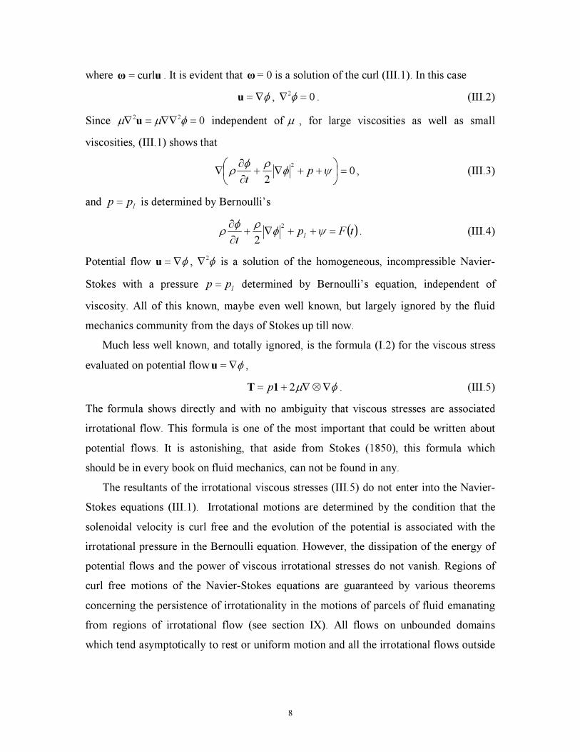
where uω curl� . It is evident that ω= 0 is a solution of the curl (III.1). In this case

��u , 02

�� . (III.2)

Since 022

�� u independent of � , for large viscosities as well as small

viscosities, (III.1) shows that

02

2

��

��

��

��

�� p

t, (III.3)

and I

pp � is determined by Bernoulli’s

� �tFpt

I��

�

��

��

2

2. (III.4)

Potential flow ��u , �2� is a solution of the homogeneous, incompressible Navier-

Stokes with a pressure I

pp � determined by Bernoulli’s equation, independent of

viscosity. All of this known, maybe even well known, but largely ignored by the fluid

mechanics community from the days of Stokes up till now.

Much less well known, and totally ignored, is the formula (I.2) for the viscous stress

evaluated on potential flow ��u ,

�� 21T p . (III.5)

The formula shows directly and with no ambiguity that viscous stresses are associated

irrotational flow. This formula is one of the most important that could be written about

potential flows. It is astonishing, that aside from Stokes (1850), this formula which

should be in every book on fluid mechanics, can not be found in any.

The resultants of the irrotational viscous stresses (III.5) do not enter into the Navier-

Stokes equations (III.1). Irrotational motions are determined by the condition that the

solenoidal velocity is curl free and the evolution of the potential is associated with the

irrotational pressure in the Bernoulli equation. However, the dissipation of the energy of

potential flows and the power of viscous irrotational stresses do not vanish. Regions of

curl free motions of the Navier-Stokes equations are guaranteed by various theorems

concerning the persistence of irrotationality in the motions of parcels of fluid emanating

from regions of irrotational flow (see section IX). All flows on unbounded domains

which tend asymptotically to rest or uniform motion and all the irrotational flows outside

9

of vorticity boundary layers give rise to an additional irrotational viscous dissipation

which deserves consideration.

The effects of viscous irrotational stresses which are balanced internally enter into the

dynamics of motion at places where they become unbalanced such as at free surfaces and

at the boundary of regions in which vorticity is important such as boundary layers and

even at internal points in the liquid at which stress induced tensions exceed the breaking

strength of the liquid. Irrotational viscous stresses enter as an important element in a

theory of stress induced cavitation in which the field of principal stresses which

determine the places and times at which the tensile stress exceed the breaking strength or

cavitation threshold of the liquid must be computed (see Funada, Wang & Joseph 2005

and Padrino, Joseph, Wang & Funada 2005).

Irrotational flows cannot satisfy no-slip and associated conditions at boundaries when

0�� (and also when 0�� ). No real fluid has 0�� . It is an act of self deception to put

away no-slip by positing a fictitious fluid which has no viscosity.

Irrotational flows of a viscous fluid scale with the Reynolds number as do rotational

solutions of the Navier-Stokes equations generally. The solutions of the Navier-Stokes

equations, rotational and irrotational, are thought to become independent of the Reynolds

number at large Reynolds numbers. They can be said to converge to a common set of

solutions corresponding to irrotational motion of an inviscid fluid. This limit should be

thought to correspond a condition of flow, large Reynolds numbers, and not to a weird

material without viscosity; the viscosity should not be put to zero.

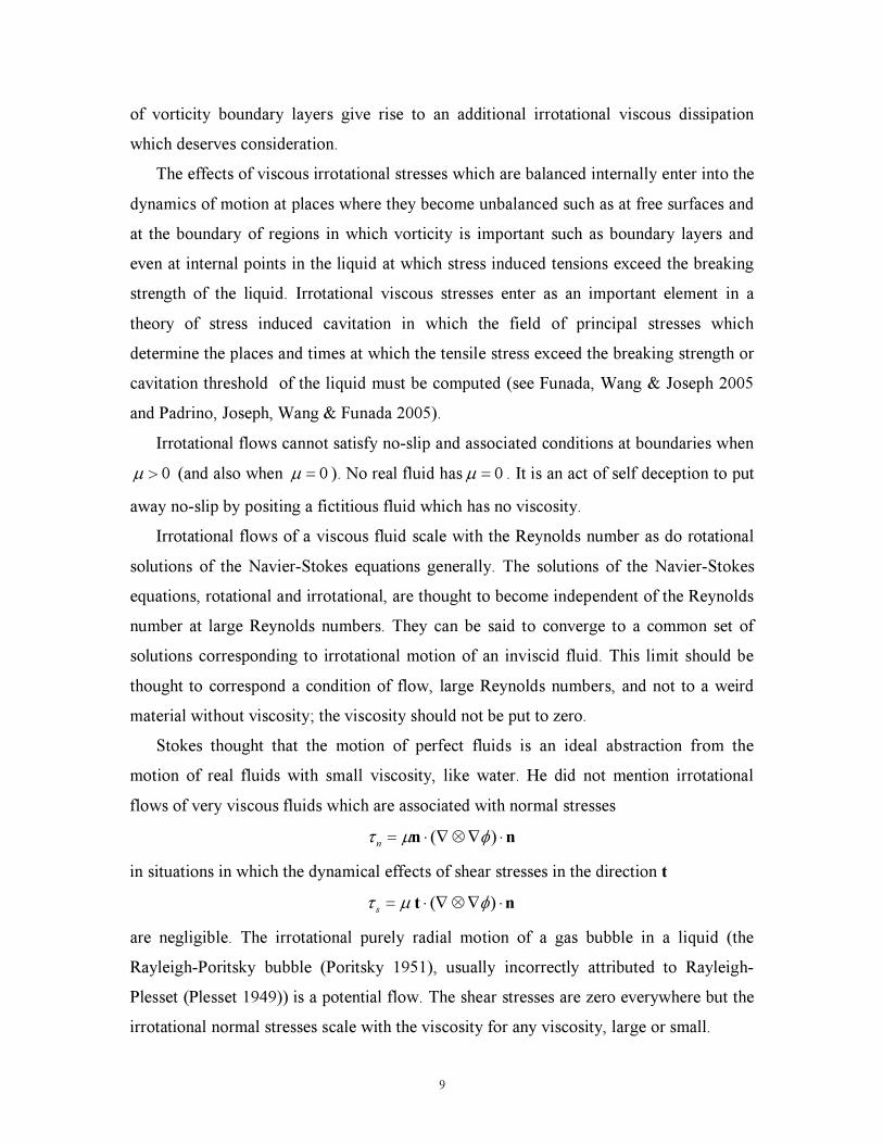
Stokes thought that the motion of perfect fluids is an ideal abstraction from the

motion of real fluids with small viscosity, like water. He did not mention irrotational

flows of very viscous fluids which are associated with normal stresses

nn �� )( ��n

in situations in which the dynamical effects of shear stresses in the direction t

nt �� )( ��s

are negligible. The irrotational purely radial motion of a gas bubble in a liquid (the

Rayleigh-Poritsky bubble (Poritsky 1951), usually incorrectly attributed to Rayleigh-

Plesset (Plesset 1949)) is a potential flow. The shear stresses are zero everywhere but the

irrotational normal stresses scale with the viscosity for any viscosity, large or small.

10

Another exact irrotational solution of the Navier Stokes equations is the flow between

rotating cylinders in which the angular velocities of the cylinders are adjusted to fit the

potential solution in circles with

.//

,

22rbrau

u

ba��

�

��

� eu

The torques necessary to drive the cylinders are proportional to the viscosity of the liquid

for any viscosity, large or small. This motion may be realized approximately in a cylinder

of large height with a free surface on top anchored in a bath of mercury below.

A less special example is embedded in almost every complex flow of a viscous fluid

at each and every stagnation point. The flow at a point of stagnation is a purely

extensional flow, a potential flow with extensional stresses proportional to the product of

viscosity times the rate extension there. The irrotational viscous extensional stresses at

points of extension can be huge even when the viscosity is small.

A somewhat more complex set of flows of viscous fluids which are very nearly

irrotational are generated by waves on free surfaces. The shear stresses on the free

surfaces vanish but the normal stresses generated by the up and down motion of the

waves do not vanish; gravity waves on highly viscous fluids are greatly retarded by

viscosity. It is not immediately obvious that the effects of vorticity on such waves are so

well approximated by purely irrotational motions (see Lamb 1932 and Wang and Joseph

2005). Very rich theories of common irrotational flows of a viscous fluid which update

and greatly improve conventional studies of perfect fluids are assembled and can be

downloaded from PDF files at

(http://www.aem.umn.edu/people/faculty/joseph/ViscousPotentialFlow/).

IV. Irrotational solutions of the compressible Navier-Stokes equations

and the equations of motion for certain viscoelastic fluids.

The velocity may be obtained from a potential provided that the vorticity ζ=curl u=0

at all points in a simply connected region. This is a kinematic condition which may or

may not be compatible with the equations of motion. For example, if the viscosity varies

with position or the body forces are not potential, then extra terms, not containing the

vorticity will appear in the vorticity equation and ζ=0 will not be a solution in general.

11

Joseph and Liao 1994 formulated a compatibility condition for irrotational solutions

��u of (I.1) in the form

� �uTu

div1

gradd

d

�� x

t

(IV.1)

If

� � ��

��Tdiv1

, (IV.2)

the 0�ζ is a solution of (IV.1) and

� �tft

��

��

��

��

��

2

2

1 (IV.3)

is the Bernoulli equation.

Consider first (Joseph 2003) the case of viscous compressible flow for which the

stress is given by (I.2). The gradient of density and viscosity which are spoiler for the

general Vorticity equation do not enter the equations which perturb uniform states of

pressure 0p , density

0� and velocity

0U .

To study acoustic propagation, the equations are linearized; putting

� � � �� 00

,,,, pppp uu , (IV.4)

where u� , p� and � � are small quantities, we obtain

��

�

�

��

�

�

�

��

�

��

�

��

� ��i

j

j

i

ijijx

u

x

uppT

000div

3

2�� u , (IV.5)

��

��

� ��

��

��

�

��uu

u

div3

12

00�� p

t, (IV.6)

0div0

��

��u�

�

t

, (IV.7)

where 0p ,

0� and

0� are constants. For acoustic problems, we assume that a small

change in � induces small changes in p by fast adiabatic processes; hence

� ��2

0Cp , (IV.8)

where 0

C is the speed of sound.

Forming now the curl of (IV.6) we find that 0curl ��u is a solution and ��u .

This gives rise to a viscosity dependent Bernoulli equation

12

� �tft

��

��

��

��

��0

,

where

�� 2

0

3

4�� .

*

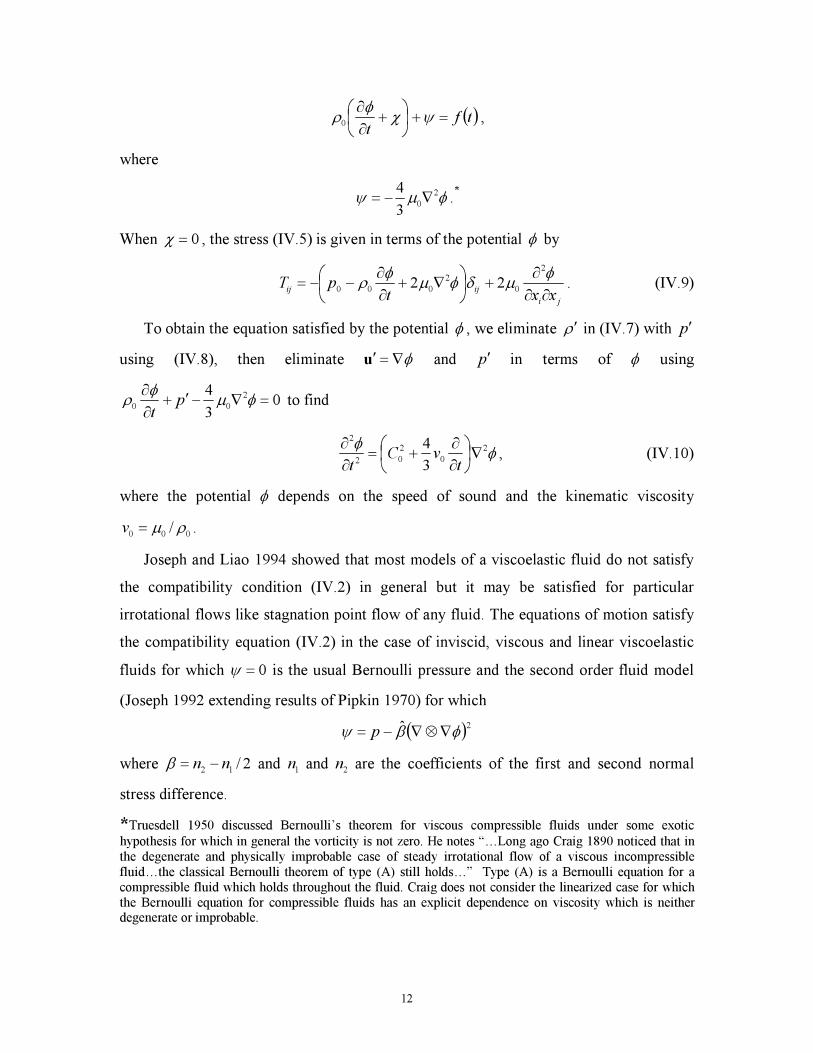
When 0�� , the stress (IV.5) is given in terms of the potential � by

ji

ijijxxt

pT��

��

�

��

��

�

��

��

��

2

0

2

00022 . (IV.9)

To obtain the equation satisfied by the potential � , we eliminate � � in (IV.7) with p�

using (IV.8), then eliminate ��u and p� in terms of � using

03

4 2

00��

�

��

�� p

t to find

�� 2

0

2

02

2

3

4��

��

�

�

�

�

�

tvC

t, (IV.10)

where the potential � depends on the speed of sound and the kinematic viscosity

000/ ��v .

Joseph and Liao 1994 showed that most models of a viscoelastic fluid do not satisfy

the compatibility condition (IV.2) in general but it may be satisfied for particular

irrotational flows like stagnation point flow of any fluid. The equations of motion satisfy

the compatibility equation (IV.2) in the case of inviscid, viscous and linear viscoelastic

fluids for which 0�� is the usual Bernoulli pressure and the second order fluid model

(Joseph 1992 extending results of Pipkin 1970) for which

� �2ˆ �� p

where 2/12nn �� and

1n and

2n are the coefficients of the first and second normal

stress difference.

*Truesdell 1950 discussed Bernoulli’s theorem for viscous compressible fluids under some exotic

hypothesis for which in general the vorticity is not zero. He notes “…Long ago Craig 1890 noticed that in

the degenerate and physically improbable case of steady irrotational flow of a viscous incompressible

fluid…the classical Bernoulli theorem of type (A) still holds…” Type (A) is a Bernoulli equation for a

compressible fluid which holds throughout the fluid. Craig does not consider the linearized case for which

the Bernoulli equation for compressible fluids has an explicit dependence on viscosity which is neither degenerate or improbable.

13

V. Irrotational solutions of the Navier-Stokes equations: viscous

contributions to the pressure

A viscous contribution to the pressure in irrotational flow is a new idea which is

required to resolve the discrepancy between the direct VPF calculation of the decay of an

irrotational wave and the calculation based on the dissipation method. The calculation by

VPF differs from the calculation based on potential flow of an inviscid fluid because the

viscous component of the normal stress at the free surface is included in the normal stress

balance. The viscous component of the normal stress is evaluated on potential flow. The

dissipation calculation starts from the evolution of energy equation in which the

dissipation integral is evaluated on the irrotational flow; the pressure does not enter into

this evaluation. Why does the decay rate computed by these two methods give rise to

different values? The answer to this question is associated with a viscous correction of

the irrotational pressure which is induced by the uncompensated irrotational shear stress

at the free surface; the shear stress should be zero there but the irrotational shear stress,

proportional to viscosity, is not zero. The irrotational shear stress cannot be made to

vanish in potential flow but the explicit appearance of this shear stress in the traction

integral in the energy balance can be eliminated in the mean by the selection of an

irrotational pressure which depends on viscosity.

The idea of a viscous contribution to the pressure seems to have been first suggested

to D. Moore 1963 by G. Batchelor as a method of reconciling the discrepancy in the

values of the drag on a spherical gas bubble calculated on irrotational flow by the

dissipation method and directly by VPF (section XI ). The first successful calculation of

this extra pressure was carried out for the spherical bubble by Kang and Leal 1988a,b.

Their work suggested that this extra viscous pressure could be calculated from

irrotational flow without reference to boundary layers or vorticity. This idea was first

implemented by Joseph and Wang 2004 using an energy argument in which the viscous

pressure was selected to eliminate the uncompensated irrotational shear stress from the

power of traction integral at the bubble surface. The idea was further developed by Wang

and Joseph 2005 in their study of viscous decay of irrotational gravity waves that showed

that this viscous contribution to the pressure could be calculated from a purely

irrotational theory. Their study is valuable because it can be compared with the exact

14

solution of Lamb 1932 in which boundary layers and vorticity are present but not

important.

Purely irrotational theories of the effect of the viscosity on the decay of free gravity waves

J. Wang and D. D. Joseph

January, 2005

Abstract

A purely irrotational theory of the effect of viscosity on the decay of free gravity waves is derived and

shown to be in excellent agreement with Lamb’s (1932) exact solution. The agreement is achieved for all

waves numbers k excluding a small interval around a critical k=kc where progressive waves change to

monotonic decay. Very detailed comparisons are made between the purely irrotational and exact theory.

1. Introduction

Lamb (1932, §348, §349) performed an analysis of the effect of viscosity on free gravity waves. He

computed the decay rate by a dissipation method using the irrotational flow only. He also constructed an

exact solution for this problem, which satisfies both the normal and shear stress conditions at the interface.

Joseph and Wang (2004) studied Lamb’s problem using the theory of viscous potential flow (VPF) and

obtained a dispersion relation which gives rise to both the decay rate and wave-velocity. They also

computed a viscous correction for the irrotational pressure and used this pressure correction in the normal

stress balance to obtain another dispersion relation. This method is called a viscous correction of the

viscous potential flow (VCVPF). Since VCVPF is an irrotational theory the shear stress cannot be made to vanish. However, the corrected pressure eliminates this uncompensated shear stress from the power of

traction integral arising in an energy analysis of the irrotational flow.

Here we find that the viscous pressure correction of the irrotational motion gives rise to a higher order

irrotational correction to the irrotational velocity which is proportional to the viscosity and does not have a

boundary layer structure. The corrected velocity depends strongly on viscosity and is not related to

vorticity; the whole package is purely irrotational. The corrected irrotational flow gives rise to a dispersion

relation which is in splendid agreement with Lamb’s exact solution, which has no explicit viscous pressure.

The agreement with the exact solution holds for fluids even 104 times more viscous than water and for

small and large wave numbers where the cutoff wave number kc marks the place where progressive waves

give rise to monotonic decay. We find that VCVPF gives rise to the same decay rate as in Lamb’s exact

solution and in his dissipation calculation when k < kc. The exact solution agrees with VPF when k > kc.

The effects of vorticity are sensible only in a small interval centered on the cutoff wave number. We will do a comprehensive comparison for the decay rate and wave-velocity given by Lamb’s exact solution and

Joseph and Wang’s VPF and VCVPF theories.

2. Irrotational viscous corrections for the potential flow solution

The gravity wave problem is governed by the continuity equation

0�� u , (1)

and the linearized Navier-Stokes equation

ue

u 21��

�

��

�y

gpt

, (2)

with the boundary conditions at the free surface (y � 0)

0�xy

T , 0�yy

T , (3)

where Txy and Tyy are components of the stress tensor and the surface tension is neglected. We divide the

velocity and pressure field into two parts

u=up+uv, p=pp+pv, (4) where the subscript p denotes potential solutions and v denotes viscous corrections. The potential solutions

satisfy

up= �� , 02

�� , (5)

15

and

ygp

te

u

��

�

p

p 1

�

. (6)

The viscous corrections are governed by

0v�� u , (7)

v

2

v

v1

u

u

��

��

�p

t

. (8)

We take the divergence of (8) and obtain

0v

2�� p , (9)

which shows that the pressure correction must be harmonic. Next we introduce a stream function ψ so that

(7) is satisfied identically:

yu

�

��

�

v

, x�

��

�

vv

. (10)

We eliminate pv from (8) by cross differentiation and obtain following equation for the stream function

��42

��

�

t

. (11)

To determine the normal modes which are periodic in respect of x with a prescribed wave-length λ=2π/ k,

we assume a time-factor ent, and a space-fact e

ikx

mykxntB ee

i�� , (12)

where m is to be determined from (11). Inserting (12) into (11), we obtain

� � 0)()(2222

�� kmnkm � . (13)

The root m2=k

2 gives rise to irrotational flow; the root �/

22nkm �� leads to the rotational component of

the flow. The rotational component cannot give rise to a non-zero harmonic pressure because mykxntmykxnt

km ee)(eei22i2 ��

�� (14)

can not vanish if m2 ≠ k

2. The only harmonic pressure for the rotational component is zero. Thus the

governing equation for the rotational part of the flow can be written as

�� 2

��

�

t

, (15)

which is the equation used by Lamb (1932) in his exact solution.

The effect of viscosity on the decay of a free gravity wave can be approximated by a purely irrotational

theory in which the explicit dependence of the power of traction of the irrotational shear stress is eliminated

by a viscous contribution pv to irrotational pressure. In this theory u=�� and a stream function, which is

associated with vorticity, is not introduced. The kinetic energy, potential energy and dissipation of the flow can be computed using the potential flow solution

kxkyntA

ie

��

�� . (16)

We insert the potential flow solution into the mechanical energy equation

� � ��

� �

Vxyyy

VVxupxgV

td :2d )(vd 2/d 2/

d

d

00

22

DDu ��

, (17)

where � is the elevation of the surface and D is the rate of strain tensor. Motivated by previous authors (Moore 1963, Kang and Leal 1988), we add a pressure correction to the normal stress which satisfies

��

��

�00

vd d )(v xuxp

xy, (18)

But in our problem here, there is no explicit viscous pressure function in the exact solution [see (24) and

(25)]. It turns out that the pressure correction defined here in the purely irrotational flow is related to

quantities in the exact solution in a complicated way which requires further analysis [see (31)]. Joseph and Wang (2004) solved for the harmonic pressure correction from (9), then determined the

constant in the expression of pv using (18), and obtained kxkyntAkp i2

ve2

��

�� . (19)

The velocity correction associated with this pressure correction can be solved from (8). We seek normal

modes solution kxkynt i

ve~

��

u and equation (8) becomes

vvpn ��u� . (20)

16

Hence, curl(uv) = 0 and uv is irrotational. After assuming 1v��u and kxkynt

Ai

11e

��

�� , we obtain

��

v1pn�� kxkynt

An

k i

2

1e

2��

�

�

�� . (21)

We compute the viscous normal stress due to the velocity correction

kxkyntAn

k

yy

i

42

2

1

2

ve

42

v2

��

��

��

�

�

�

�� . (22)

Since for mobile fluids such as water or even glycerin, �=µ/ρ is small, this viscous normal stress is negligible compared to pv when k is small. Therefore, the viscous normal stress induced by the velocity

correction can be neglected in the normal stress balance in the VPVPF theory. The viscous normal stress

(22) could be large when k is large, however, we will show in the following sections that the flow is nearly

irrotational at large values of k and no correction is needed.

The calculation shows that the velocity correction uv associated with the pressure correction is

irrotational. Our pressure correction (19) is proportional to µ and on the same order of the viscous stresses

evaluated using � (16). This pressure correction is associated with a correction for the velocity potential �1

(21), which is also proportional to µ. The shear stress evaluated using �1 is proportional to µ2 and non-zero.

To balance the power of this non-physical shear stress, one can add a pressure correction proportional to µ2,

which will in turn induce a correction for the velocity potential proportional to µ2. One can continue to

build higher order corrections and they will all be irrotational. The final velocity potential has the following

form kxkynt

AAAi

21e)(

��

�� , (23)

where A1�µ, A2�µ2... Thus the VCVPF theory is an approximation to the exact solution based on solely

potential flow solutions. The higher order corrections are small for liquids with small viscosities; the most

important correction is the first pressure correction proportional to µ. In our application of VCPVF to the

gravity wave problem, only the first pressure correction (19) is added to the normal stress balance and

higher order normal stress terms such as (22) are not added. We obtain a dispersion relation in excellent

agreement with Lamb’s exact solution (see the comparison in the next section); adding the higher order

corrections to the normal stress balance does not improve the VCVPF approximation. It should be pointed

out that no matter how many correction terms are added to the potential (23), the shear stress evaluated

using (23) is still non-zero unless (A + A1 + A2 + ...) = 0. Therefore, VCVPF is only an approximation to the

exact solution and cannot satisfy the shear stress condition at the free surface.

VI. Irrotational solutions of the Navier-Stokes equations: classical

theorems.

An authorative and readable exposition of irrotational flow theory and its applications

can be found in chapter 6 of the book on fluid dynamics by G.K. Batchelor 1967. He

speaks of the role of the theory of flow of an inviscid fluid. He says

In this and the following chapter, various aspects of the flow of a fluid regarded as entirely inviscid

(and incompressible) will be considered. The results presented are significant only inasmuch as they

represent an approximation to the flow of a real fluid at large Reynolds number, and the limitations of each

result must be regarded as information as the result itself.

Most of the classical theorems reviewed in Chapter 6 do not require that the fluid be

inviscid. These theorems are as true for viscous potential flow as they are for inviscid

potential flow. Kelvin’s minimum energy theorem holds for the irrotational flow of a

viscous fluid. The results for the positions of the maximum speed the minimum of the

17

pressure given by the Bernoulli equation follow from the assumption that the flow is

irrotational independent of the viscosity of the fluid.

The theory of the acceleration reaction leads to the concept of added mass; it follows

from the analysis of unsteady irrotational flow. The theory applies to viscous and inviscid

fluids alike.

Harold Jeffrey 1928 derived an equation (his (20)) which replaces the circulation

theorem of classical (inviscid) hydrodynamics. When the fluid is homogeneous, Jeffrey’s

equation may be written as

� �� lω dt

Ccurl

d

d

�

� (VI.1)

where

� � � �� lu dtC

is the circulation round a closed material curve drawn in the fluid. This equation shows

that

“… the initial value of tC d/d around a contour in a fluid originally moving irrotationally is zero, whether

or not there is a moving solid within the contour. This at once provides an explanation of the equality of the

circulation about an aero plane and that about the vortex left behind when it starts; for the circulation about

a large contour that has never been cut by the moving solid or its wake remains zero, and therefore the

circulations about contours obtained by subdividing it must also add up to zero. It also indicates why the

motion is in general nearly irrotational except close to a solid or to fluid that has passed near one”.

St. Venant 1869 interpreted the result of Lagrange about the invariance of circulation

0d/d �tC to mean that

vorticity cannot be generated in the interior of a viscous incompressible fluid, subject to conservative

extraneous force, but is necessarily diffused inward from the boundaries.

The circulation formula (VI.1) is an important result in the theory of irrotational flows

of a viscous fluid. A particle which is initially irrotational will remain irrotational in

motions which do not enter into the vortical layers at the boundary.

VII. Critical remarks about the “The impossibility of irrotational motions

in general”.

This topic is treated in § 37 of the monograph by Truesdell 1954. The basic idea is

that, in general, irrotational motions of incompressible fluids satisfy Laplace’s equation

18

and the normal and tangential velocities at the bounding surfaces can not be

simultaneously prescribed. The words “in general” allow for rather special cases in which

the motion of the bounding surfaces just happens to coincide with the velocities given by

the derivatives of the potential. Such special motions were studied for viscous

incompressible fluids by Hamel 1941. A bounding surface must always contact the fluid

so the normal component of the velocity of the fluid must be exactly the same as the

normal component of the velocity of the boundary. The no-slip condition cannot then “in

general” be prescribed. Truesdell uses “adherence condition” meaning “sticks fast” rather

than the usual no-slip condition of Stokes. The no slip condition is even now a topic of

discussion and the mechanisms by which fluids stick fast are not clear. Truesdell does not

consider liquid-gas surfaces or, more exactly, liquid-vacuum surfaces on which slip is

allowed.

Truesdell’s conclusion

“…that the boundary condition customarily employed in the theory of viscous fluids makes irrotational motion is a virtual impossibility.”

is hard to reconcile with the idea that flows outside boundary layers, are asymptotically

irrotational. Ever so many examples of non-exotic calculations of irrotational motions of

viscous fluids which approximate exact solutions of the Navier-Stokes equations and

even agree with experiments at low Reynolds numbers are listed on Joseph’s web based

archive.

VIII. The drag on a spherical gas bubble

As in the case of irrotational waves, the problem of the drag on gas bubbles in a

viscous liquid may be studied using viscous potential flow directly and by the dissipation

method and the two calculations do not agree.

The idea that viscous forces in regions of potential flow may actually dominate the

dissipation of energy was first expressed by Stokes 1950, and then, with more details, by

Lamb 1932 who studied the viscous decay of free oscillatory waves on deep water § 348

and small oscillations of a mass of liquid about the spherical form § 355, using the

dissipation method. Lamb showed that in these cases the rate of dissipation can be

calculated with sufficient accuracy by regarding the motion as irrotational.

19

VIII.1 Dissipation calculation. The computation of the drag D on a sphere in potential

flow using the dissipation method seems to have been given first by Bateman in 1932

(see Dryden, Murnaghan and Bateman 1956) and repeated by Ackeret 1952. They found

that UaD ��12� where � is the viscosity, a radius of the sphere and U its velocity. This

drag is twice the Stokes drag and is in better agreement with the measured drag for

Reynolds numbers in excess of about 8.

The same calculation for a rising spherical gas bubble was given by Levich 1949.

Measured values of the drag on spherical gas bubbles are close to Ua��12 for Reynolds

numbers larger than about 20. The reasons for the success of the dissipation method in

predicting the drag on gas bubbles have to do with the fact that vorticity is confined to

thin layers and the contribution of this vorticity to the drag is smaller in the case of gas

bubbles, where the shear traction rather than the relative velocity must vanish on the

surface of the sphere. A good explanation was given by Levich 1962 and by Moore 1959,

1963; a convenient reference is Batchelor 1967. Brabston and Keller 1975 did a direct

numerical simulation of the drag on a gas spherical bubble in steady ascent at terminal

velocity U in a Newtonian fluid and found the same kind of agreement with experiments.

In fact, the agreement between experiments and potential flow calculations using the

dissipation method are fairly good for Reynolds numbers as small as 5 and improves

(rather than deteriorates) as the Reynolds number increases.

The idea that viscosity may act strongly in the regions in which vorticity is effectively

zero appears to contradict explanations of boundary layers which have appeared

repeatedly since Prandtl. For example, Glauert 1943 says (p.142) that

… Prandtl’s conception of the problem is that the effect of the viscosity is important only in a narrow

boundary layer surrounding the surface of the body and that the viscosity may be ignored in the free fluid

outside this layer.

According to Harper 1972, this view of boundary layers is correct for solid spheres

but not for spherical bubbles. He says that

… for R>>1, the theories of motion past solid spheres and tangentially stress-free bubbles are quite

different. It is easy to see why this must be so. In either case vorticity must be generated at the surface

because irrotational flow does not satisfy all the boundary conditions. The vorticity remains within a

boundary layer of thickness � �2/1�� aRO� , for it is convected around the surface in a time t of order a/U,

during which viscosity can diffuse it away to a distance � if � � � �RaOtO /22

�� . But for a solid sphere

20

the fluid velocity must change by � �UO across the layer, because it vanishes on the sphere, whereas for a

gas bubble the normal derivative of velocity must change by � �aUO / in order that the shear stress be zero.

That implies that the velocity itself changes by � � � � � �UoUROaUO ��

� 2/1/� …

In the boundary layer on the bubble, therefore, the fluid velocity is only slightly perturbed from that of

the irrotational flow, and velocity derivatives are of the same order as in the irrotational flow. Then the

viscous dissipation integral has the same value as in the irrotational flow, to the first order, because the total

volume of the boundary layer, of order �2

a , is much less than the volume, of order 3a , of the region in

which the velocity derivatives are of order aU / . The volume of the wake is not small, but the velocity

derivatives in it are, and it contributes to the dissipation only in higher order terms….

The drag on a spherical gas bubble in steady flow at modestly high Reynolds numbers

(say, 50�e

R ) can be calculated using the dissipation method assuming irrotational flow

without any reference to boundary layers or vorticity. The dissipation calculation gives

UaD ��12� or RCD

/48� where �� /2aUR � .

VIII.2 Direct calculation of the drag using viscous potential flow (VPF). Moore 1959

calculated the drag directly by integrating the pressure and viscous normal stress of the

potential flow. The irrotational shear stress is not zero but is not used in the drag

calculation. The shear stress which is zero in the real flow was put to zero in the direct

calculation. The pressure is computed from Bernoulli’s equation and it has no drag

resultant. If the irrotational shear stress was not neglected the drag by direct calculation

would vanish, even though the dissipation is not zero. Moore’s direct calculation gave

UaD ��8� or RCD

/32� instead of RCD

/48� .

VIII.3 Pressure correction (VCVPF). The discrepancy between the dissipation

calculation leading to RCD

/48� and the direct VPF calculation leading to RCD

/32�

led G. K. Batchelor, as reported in Moore 1963, to suggest the idea of a pressure

correction to the irrotational pressure. In that paper, Moore performed a boundary layer

analysis and his pressure correction is readily obtained by setting y = 0 in his equation

(2.37):

� � � ��

�cos2cos1

sin

4 2

2��

Rp , (VIII.1)

which is singular at the separation point where �� . The presence of separation is a

problem for the application of boundary layers to the calculation of drag on solid bodies.

21

To find the drag coefficient Moore calculated the momentum defect, and obtained the

Levich value 48/R plus contributions of order R-3/2 or lower.

The first successful calculation of a viscous pressure correction was carried out by

Kang and Leal 1988a. They calculated a viscous correction of the irrotational pressure by

solving the Navier-Stokes equations under the condition that the shear stress on the

bubble surface is zero. Their calculation could not be carried out to very high Reynolds

numbers, and it was not verified that the dissipation in the liquid is close to the value

given by potential flow. They find indications of a boundary layer structure but they do

not establish the existence of properties of a layer in which the vorticity is important.

They obtain the drag coefficient 48/R by direct integration of the normal stress and

viscous pressure over the boundary. This shows that the force resultant of the pressure

correction does indeed contribute exactly the 16/R which is needed to reconcile the

difference between the dissipation calculation and the direct calculation of drag.

Kang and Leal 1988a obtain their drag result by expanding the pressure correction as

a spherical harmonic series and noting that only one term of this series contributes to the

drag, no appeal to the boundary layer approximation being necessary. Kang and Leal

1988b remark that

“In the present analysis, we therefore use an alternative method which is equivalent to Lamb’s

dissipation method, in which we ignore the boundary layer and use the potential flow solution right up to

the boundary, with the effect of viscosity included by adding a viscous pressure correction and the viscous

stress term to the normal stress balance, using the inviscid flow solution to estimate their values.”

The VCVPF approach to problems of gas-liquid flows taken by Joseph and Wang

2004 and by Wang and Joseph 2005, in which the viscous contribution to the pressure is

selected to remove the uncompensated irrotational shear stress from the traction integral

(see VIII.18), is different than that used by Kang and Leal 1988a, b.

For the case of a gas bubble rising with the velocity U in a viscous fluid, it is possible

to prove that the drag D1 computed indirectly by the dissipation method is equal to the

drag D2 computed directly by our formulation of VCVPF. Suppose that (VIII.18) holds

and that the drag on the bubble is given as D1 = Ɗ /U, where Ɗ is the dissipation. Then

D1 = Ɗ /U

� � ��

V A

UAunUV /d2/d:2 DDD ��

22

� � � �� A A

nn

v

ssnnUAupUAuu /d/d ��

�� A

nxn

iv

Anx

DAeeAppee2

d)d( T�

where we have used the normal velocity continuity nxneUeu �� , the zero-shear-stress

condition at the gas-liquid interface and the fact that the Bernoulli pressure does not

contribute to the drag.

Dissipation calculations for the drag on a rising oblate ellipsoidal bubble was given

by Moore 1965 and for the rise of a spherical liquid drop, approximated by Hill’s

spherical vortex in another liquid in irrotational motion. The drag results from these

dissipation calculations were obtained by Joseph and Wang 2004, using the VCVPF

pressure correction formula (VIII.18).

VIII.4 Acceleration of a spherical gas bubble to steady flow. A spherical gas bubble

accelerates to steady motion in an irrotational flow of a viscous liquid induced by a

balance of the acceleration of the added mass of the liquid with the Levich drag. The

equation of rectilinear motion is linear and may be integrated giving rise to exponential

decay with decay constant 218 t a� � where � is the kinematic viscosity of the liquid and

a is the bubble radius. The problem of decay to rest of a bubble moving initially when

the forces maintaining motion are inactivated and the acceleration of a bubble initially at

rest to terminal velocity are considered. The equation of motion follows from the

assumption that the motion of the viscous liquid is irrotational. It is an elementary

example of how potential flows can be used to study the unsteady motions of a viscous

liquid suitable for the instruction of undergraduate students.

Consider a body moving with the velocity U in an unbounded viscous potential flow.

Let M be the mass of the body and M � be the added mass, then the total kinetic energy

of the fluid and body is

21( )

2T M M U�� (VIII.2)

Let D be the drag and F be the external force in the direction of motion, then the power

of D and F should be equal to the rate of the total kinetic energy,

d d( ) ( )

d d

T UF D U M M U

t t�� (VIII.3)

23

We next consider a spherical gas bubble, for which 0M � and 32

3fM a� �� . The drag

can be obtained by direct integration using the irrotational viscous normal stress and a

viscous pressure correction: 12D aU�� . Suppose the external force just balances the

drag, then the bubble moves with a constant velocity 0

U U� . Imagine that the external

force suddenly disappears, then (VIII.3) gives rise to

32 d12

3 df

UaU a

t�� (VIII.4)

The solution is 18

2

0e

a

t

U U

��

� � (VIII.5)

which shows that the velocity of the bubble approaches zero exponentially.

If gravity is considered, then 34

3fF a g� �� . Suppose the bubble is at rest at 0t � and

starts to move due to the buoyant force. Equation (VIII.3) can be written as

3 34 2 d12

3 3 df f

Ua g aU a

t� � �� (VIII.6)

The solution is

18

2

2

1 e9

a

ta gU

�

�

� ��

� � � (VIII.7)

which indicates the bubble velocity approaches the steady state velocity

2

9

a gU

�

� . (VIII.8)

VIII.5 The rise velocity and deformation of a gas bubble computed using VPF. The

shape of a rising bubble, or of a falling drop, in an incompressible viscous liquid was

computed numerically by Miksis, Vanden-Broeck and Keller 1982, omitting the

condition on the tangential traction at the bubble or drop surface. The shape is found,

together with the flow of the surrounding fluid, by assuming that both are steady and

axially symmetric, with the Reynolds number being large. The flow is taken to be a

potential flow and the viscous normal stress, evaluated on the irrotational flow, is

included in the normal stress balance. This study is exactly what we have called VPF; it

24

follows the earlier study of Moore 1957, but it differs markedly from Moore’s study

because the bubble shape is computed.

When the bubble is sufficiently distorted, its top is found to be spherical and its

bottom is found to be rather flat. Then the radius of its upper surface is in fair agreement

with the formula of Davies and Taylor 1950. This distortion occurs when the effect of

gravity is large while that of surface tension is small. When the effect of surface tension

is large, the bubble is nearly a sphere. The difference in these two cases is associated with

large and small Morton numbers.

VIII.6 The rise velocity of a spherical cap bubble computed using VPF. Davies and

Taylor 1950 studied the rise velocity of a lenticular or spherical cap bubble assuming that

motion was irrotational and the liquid inviscid. The spherical cap as if some fraction of

the sphere much less than 1/2, say 1/8, is cut off with the spherical cap in the front and a

nearly flat trailing edge. These are the shapes of large volume bubbles of gas rising in the

liquid. They measured the bubble shape and showed that it indeed had a spherical cap

when rising in water. Brown 1965 did experiments which shows the cap is very nearly

spherical even when the liquid in which the gas bubble rises is very viscous.

Joseph (2002) applied the theory of viscous potential flow VPF to the problem of

finding the rise velocity U of a spherical cap bubble. The rise velocity is given by

gD

U=

2/1

3

2

3

321

3

2

3

8

��

��

��gD

v

gD

v, (VIII.9)

where R = D/2 is the radius of the cap and v is the kinematic viscosity of the liquid.

Davies and Taylor’s 1950 result follows from (VIII.9) when the viscosity is zero.

Equation (VIII.9) may be expressed as a drag law

CD = 6 + 32/Re. (VIII.10)

This drag law is in excellent agreement with experiments at large Morton numbers

reported by Bhaga and Weber 1981 after the drag law is scaled so that the effective

diameter used in the experiments and the spherical cap radius of Davies and Taylor 1950

are the same (see Figure 1).

25

1

10

100

1000

0.1 1 10 100 1000

R

CD

CD =0.445*(6 + 32/R)

CD =[2.67 0.9 + (16/R)0.9]1/0.9

Figure 1. Comparison of the empirical drag law with the theoretical drag law (9) scaled by the

factor 0.445 required to match the experimental data reported by Bhaga and Weber 1981

with the experiments of Davies and Taylor 1950 at large Re. The agreement between theory

and experiment based on the irrotational flow of a viscous fluid is excellent even for Reynolds

numbers as small as 0.1.

Viscous potential flow VPF works well in the case of spherical cap bubbles, but a viscous

pressure correction VCVPF is required to bring theory and experiment together in the

case of small spherical gas bubbles. This is like the problem of the effect of viscosity on

the decay of irrotational gravity waves studied by Lamb 1932 and Wang and Joseph 2005

in which the decay of long waves is correctly predicted by VCVPF and the decay of short

waves is correctly predicted by VPF.

IX Dissipation and drag in irrotational motions over solid bodies Contrived examples of irrotational motions of viscous fluids over solid bodies are

those in which it is imagined that the boundary of the solid moves with exactly same

velocity as the potential flow. These irrotational motions are exactly the same as those in

which the viscous fluid is allowed to slip at the boundary of the solid. Some authors

claim that the drag on a solid body exerted by a viscous liquid in potential flow can be

obtained by equating the product DU of drag time’s velocity to the total dissipation in the

liquid evaluated on the potential; other authors say the drag is zero. The relation of drag

to dissipation in irrotational flow is subtle and its utility as theoretical tool depends

26

critically on understanding what to do with unphysical irrotational shear stress at the

boundary of the body.

IX.1 Energy equation. Consider the motion of a body in a fluid at rest at infinity. If there

are no body forces and the fluid is homogeneous, the evolution of the mechanical energy

is given by

� � �� SV

SpVt

d2dd

d

2

1 2

nDunuu �� Ɗ, (IX.1)

where � �uDD � ,

Ɗ VV

d:2 DD�� (IX.2)

is the dissipation, V is the region exterior to the body with surface S and normal n drawn

into the body. The stress vector on S is given by

tnnDτsn

�� 2 , (IX.3)

where nDn �� 2n

is the component of the component of the stress vector normal to S

and nDt �� 2s

is the component of stress vector tangent to S. We may write (IX.1) as

�� S snSp

t

Ε]d)([

d

dutun �� Ɗ, (IX.4)

where ��

V

VE d2

1 2

u� .

If the body a solid moving with a velocity x

Ueu � and the no-slip condition applies; it

can be shown using 0div �u , that 0�n

� and

�� DUt

E

d

dƊ, (IX.5)

where

� ��

Sxsx

StpnD d][ � (IX.6)

is the drag. For steady flow

�DU Ɗ (IX.7)

the rate of working of the drag force is balanced by dissipation.

27

IX.2 d'Alembert paradox. If 0�� , then Ɗ = 0 and 0�D . The drag of a body in an

inviscid flow vanishes. However, for irrotational flow of a viscous fluid

Ɗ ��

�

��

��

Sji

Vji

SVxxxx

dd22

22

��

� n (IX.8)

is not zero. However, if the fluid is viscous and the flow is irrotational, then, using

��u and (IX.8) we find that

0dd �� Vijij

Sjiji

VDDSnDu . (IX.9)

Hence, for steady flow, using (IX.1) and veu ��x

U ,

where 0��nv , we get

0d �� UDSpnUS

x.

It follows that in the irrotational flow of a viscous fluid over a body

0�D , (IX.10)

even though Ɗ ≠ 0. Now we have two paradoxes instead of one.

IX.3 Different interpretations of the boundary conditions for irrotational flows over

solids. Finzi 1926 calculated the dissipation due to the irrotational motion of a viscous

fluid when the fluid is allowed to slip at the boundary of a solid of unspecified shape. His

goal was to compute the drag associated with the dissipation of the irrotational flow. He

computes the dissipation as the sum of the usual volume integral of the square of the rate

of strain over the fluid times the viscosity plus the power of the irrotational viscous

stresses on the boundary. He shows that the dissipation so defined vanishes when the

velocity is harmonic as is the case for irrotational flow. Thus in Finzi’s theory there is no

dissipation of energy in irrotational flow (cf. Bateman 1956 p. 158).

Bateman 1932 computed D=12πµaU from (IX.7) for a solid sphere of radius a

moving forward with velocity U in a potential flow motionless at infinity. Exactly the

same value for drag on a spherical gas bubble was computed in exactly the same way by

Levich 1949. Levich justified his result by arguing that the drag due to the weak vorticity

boundary layer at the gas-liquid interface is much smaller than the drag due to the

dissipation of the irrotational flow. There are two ways to interpret Bateman’s result: (1)

28

the fluid slips at the solid and the dissipation is balanced by the power of the traction

leading to zero drag (IX.10) or (2) the fluid does not slip, there is a region at the boundary

which may be small or large in which vorticity is important and 12πµaU approximates

the additional drag due to the viscous dissipation in the irrotational outside the boundary

layer.

Some German researchers (Hamel 1941, Ackeret 1952, Romberg 1967 and Zierip

1984) considered the problem of dissipation and drag on solid bodies in contrived

irrotational motions of a viscous fluid. Hamel 1941 noted that though the resultants of the

viscous irrotational stresses vanish, the work done by these stresses do not vanish. This

observation motivated his discussion of dissipation and drag. The papers of Hamel and

Ackeret are very similar; they both use the formula (IX.7) relating dissipation and drag

for solid bodies under the contrived assumption (equivalent to allowing slip) that the

boundary of the solid moves with the velocity of the irrotational flow. Ackeret gives drag

results for circular cylinders in a uniform stream with circulation, for elliptic cylinders,

for spheres and other bodies. Zierep 1984 in a paper on viscous potential flow discusses

the dissipation and drag associated with the moving wall calculations of Hamel and

Ackeret; he calls this a pseudo drag which “originates from friction.” He says that “…A

real drag does not appear in potential flows including those with friction.” This friction is

due to the irrotational shear stress and it has no frictional effect in potential flows which

slip at the wall; it is not helpful to hide this slip by contriving to move a solid wall at the

precise speed of the moving wall. Zierep’s claim that the drag on a solid body in

irrotational flow vanishes is a consequence of d’Alembert’s principle for flows with a

non-zero dissipation embodied in (IX.10). Zierep’s discussion of viscous potential flow is

confused: he says that viscous potential flow is independent of the Reynolds number; he

did not discuss the irrotational viscous stresses which scale with the Reynolds number.

He notes that the drag on a sphere with a moving wall computed from (IX.7) is the same

as the drag on a spherical gas bubble computed by Levich 1949. He notes that drag on the

bubble is in good agreement with experiment and he attributes this difference to the fact

that the shear stress on the bubble surface vanishes and the gas liquid is like moving wall.

He does not confront the discrepancy posed by the non-zero viscous and irrotational

shear stress in the theory and the zero shear stress condition required in practice.

29

IX.4 Viscous dissipation in the irrotational flow outside the boundary layer and wake

The paper on dissipation and drag by G. Romberg 1967 is important and deserves to be

better known. In this paper

The connection between drag and dissipation in incompressible flows is derived. Two cases are

considered: Firstly the surface of the body is at rest and secondly the surface elements can move

.In the further case the flow outside the boundary layer and the wake contributes a term to the drag coefficient which is proportional to Reynolds number to the minus one (high Reynolds

number assumed). The coefficient of this term is completely fixed by the frictionless flow.

The dissipation in the irrotational flow of a viscous fluid outside the boundary layer had

not been considered before Romberg. I learned about this paper from Zierep 1984 who

discussed the first two topics but ignored the flow outside the boundary layer. Much later

and independently, Wang and Joseph 2005 prepared a work on pressure corrections for

the effects of viscosity on the irrotational flow outside Prandtl’s boundary layer; in one

chapter they calculated the additional drag on a Joukowski airfoil at an angle of attack by the

dissipation method.

The existence of an added drag due to viscosity in the irrotational flow outside the very small

vorticity layer at the bubble surface is widely accepted by fluid mechanics researchers. The

situation there and in other gas-liquid free surface problems is complicated by the uncompensated

irrotational shear stress at the interface which is intimately connected to the viscous action in the

irrotational flow. This complication does not appear in the equivalent formulation in which the

irrotational effects of viscosity are computed using the dissipation method. It is hard to envisage a

situation in which the viscous effects associated with irrotational gas-liquid flows do not occur in

other irrotational flows, like those outside Prandtl’s boundary layer. The effects of the shear stress

at the surface of a rigid body are well described with traditional boundary layer theory but in

flows in which the irrotational shear stresses at the edge of the boundary layer are not the same as

the ones obtained from boundary layer analysis there is mismatch which begs for resolution.

Indeed we can think that the body plus the boundary moves through the irrotational flow like a

bubble in which the resolution of discontinuous velocity derivatives rather than the resolution of a

discontinuous velocity is at issue. The simplest kind of analysis to try for the boundary layer

problem is the dissipation method where the dissipation would be computed in the region outside

the boundary layer. This approach is difficult to implement because there is no definite end to the

boundary layer and for other reasons. To avoid these difficulties, the viscous dissipation of the

30

irrotational flow could be computed everywhere outside and inside the boundary layer, right up to

the boundary as was done by Romberg 1967 and by Wang and Joseph 2005. If this approach has

merit, all the calculations of the drag and dissipation in irrotational motions around solids given

by Hamel 1941 and Ackeret 1952 which I called contrived might actually give an approximation

to the added drag due to the irrotational flow outside the boundary layer.

Romberg calculated the additional drag due to viscosity in the irrotational flow over an

ellipse at a zero angle of attack. He finds that the coefficient of the drag is given by

� �ed

RC /142

�� ,

where τ is the aspect ratio of the ellipse. The drag coefficient tends to e

R/4� as the

ellipse collapses onto its major axis. This is the flow over a flat plate. Romberg notes that

the dissipation integral (IX.8) remains finite because the integrand is singular at the front

at the front stagnation point.

Wang and Joseph 2005 computed the additional viscous drag on a Joukowski airfoil

in the well known irrotational streaming flow obtained from the conformal

transformation z=ζ+c2/ζ from a circle of radius a=c(1+ε) with circulation

�� sin40aUΓ � where β is the attack angle and ε is the sharpness parameter; the smaller

ε the sharper the nose. They calculated this drag from the dissipation integral (XII.8)

using the complex potential f(z)=φ+iψ. The drag coefficient Cd=-2I(ε,β)/Re where

Re=4cU0 /ν is given in the table just below.

Figure 2. Added drag due to the viscous dissipation in the irrotational flow outside the boundary

layer. This drag is negligible at very high Reynolds numbers

31

X. Major effects of viscosity in irrotational motions can be large; they are

not perturbations of potential flows of inviscid fluids.

At the risk of repeating myself, I feel that it is necessary to write this section

forcefully because the contrary opinion is so widespread. The best way to establish this

point is to list many examples in which viscous effects computed from purely irrotational

theories are both large and in good agreement with exact theoretical results and

experiments.

X.1 Exact solutions. By exact solutions I mean irrotational solutions which satisfy also

satisfy commonly accepted boundary conditions for viscous fluids. Irrotational flows of

viscous fluids cannot in general satisfy no-slip conditions at solid-fluid surfaces or

continuity conditions on the tangential components of velocity and stress at the interface

between liquids. At a gas-liquid surface the tangential component velocity in the liquid is

essentially unrestricted as it would be at a vacuum-liquid surface but the continuity of the

shear stress leads to the condition that the shear stress must be essentially zero in the

liquid as it is in the vacuum or nearly in the gas. I know only of two non-contrived

examples of potential flows which satisfy these strict conditions. The first is the purely

rotary flow between rotating cylinders adjusted so that the velocity of the fluid in circles

is proportional to c/r. The second solution arises in purely radial gas-liquid flows of

spherical bubbles or drops (Poritsky 1951). In these purely radial flows, shear stresses

cannot develop but irrotational viscous normal stresses proportional to the viscosity are

not zero. The irrotational solutions of these problems work for water and pitch,

independent of viscosity.

X.2 Gas-liquid flows; bubbles, drops and waves. Irrotational studies of gas-liquid flows

cannot be made to satisfy the zero shear stress condition on the free surface. This

mismatch leads to the generation of vorticity. Very often the contribution of vorticity is

confined to a boundary layer and the viscous effects in these layers are much smaller than

the viscous effects in the purely irrotational flow. The purely irrotational analysis of the

rise velocity of a spherical cap bubble described in figure 2 is in good agreement with

experiment at high Morton numbers even at Reynolds numbers of 0.1. Classical studies

32

of interfacial stability for potential flow of inviscid fluids are as easily done for the

potential flow of viscous and even viscoelastic fluids.

X.3 Rayleigh-Taylor instability. Joseph, Belanger and Beavers 1999 studied the breakup

of drops in a high speed air stream behind a shock wave. At first the drop flattens due to

high pressure at the front and back of drop. The accelerations can be 105 times gravity;

this huge acceleration is main dynamical feature for generating the RT instability which

give rise to the corrugations seen on the front face of the drop before it is set into motion

by acceleration (see figure 3). The analysis of RT instability can be done exactly from the

linearized Navier Stokes equations and from viscous potential flow VPF. The growth

rates and the wave length for maximum growth depend strongly on viscosity; the

difference between VPF and the exact solution is about 2% at most for small and large

viscosities. Similar agreement between the irrotational theory, exact solutions and

experiments for RT instability were given by Joseph, Beavers and Funada 2002.

Silicone Oil 100

0

20000

40000

60000

80000

100000

120000

140000

160000

0 500 1000 1500 2000

k

n

Water

0

20000

40000

60000

80000

100000

120000

140000

160000

0 200 400 600 800 1000

k

n

Figure 3. Growth rate curves for Rayleigh-Taylor instability for water (1cp) silicon oil (100 cp).

The critical cut off wave number is given by kc=(ρa/γ)1/2

,where a is acceleration γ is surface

tension, is independent of viscosity. The maximum value of the growth rate decreases strongly with viscosity and the maximum value of the growth rate shifts strongly to longer waves. The

growth rate curves here computed from viscous petential flow are less than 2% different than

the curves from the exact theory. The irrotational theory agrees with exact theory and with

experiments even when the viscosity is very large.

X.4 Capillary instability. Wang, Joseph and Funada 2005 studied capillary instability

using VPF and VCVPF; they compared their results to the exact solution of Tomotika

1935. The differences between the exact solution and VCVPF are at most a few percent

even for viscosities a million times larger than water. A vorticity layer exists at the

33

interface but for gas-liquid flows, its effect on the linearized dynamics is negligible. It is

unexpected that the purely irrotational analysis of capillary instability of two very viscous

liquids like Golden syrup and paraffin should give results close to the exact solution for

the shorter waves in the region of cut-off and maximum growth rates. The effects of

vorticity are not uniform in k, they are more important for long waves (small k).

0.0001

0.001

0.01

0.1

1

0.001 0.01 0.1 1 10k

�

IPF

VPF

VCVPF

Exact

Glycerin-air, R

e = 1.303

0.0001

0.001

0.01

0.1

1

0.001 0.01 0.1 1 10

k

�

IPF

VPF

VCVPF

Exact

0.0001

0.001

0.01

0.1

1

0.001 0.01 0.1 1 10

k

�

IPF

VPF

VCVPF

Exact

SO10000-air, R

e =2.035×10

-3 Goldensyrup-paraffin, R

e =2.66×10

-3

Figure 4. Growth rate curves for capillary instability of a liquid cylinder. The growth rates given

by VCVPF are in good agreement with the exact solution for all k in the case of liquids in air

(Wang, Joseph and Funada 2005a). The agreement in the two-liquid case (Wang, Joseph and Funada 2005b) is good for the maximum growth rates but poor for long waves (small k).

Similar agreements between purely irrotational analysis of capillary instability of

viscoelastic fluids and exact solutions have been obtained by Funada et al 2005.

X.5 Kelvin-Helmholtz instability. This is an instability which arises from a discontinuity

in the velocity of uniform parallel streams. It is usually studied using Euler’s equations

because the continuity of the tangential components of velocity and stress required in the

Navier- Stokes theory will not allow discontinuities Basset 1888, §518, Vortex sheets

cannot exist in a viscous liquid p.308). However, these discontinuities are compatible

with viscous potential flow. Funada and Joseph 2001 studied KH instability in a channel.

34

Funada et al. 2004 studied KH instability of a liquid jet into incompressible gases and

liquid using VPF, of the same problem using VCVPF 2005 and of a liquid cylinder in a

supersonic compressible gas 2005. The instabilities in all these studies depend strongly

on viscosity but there are no exact solutions to which they may be compared.

X.6 Free waves on highly viscous liquids. Here we return to the discussion in section

VIII of purely irrotational effects of the viscosity on the decay of free gravity waves. In

figure 5 we compare Lamb’s exact solution with the irrotational solutions VPF and

VCVPF in the case when the viscosity of the liquid is 108 larger than water. The exact

solution and the irrotational solutions are in good agreement uniformly in k except near

the critical value kc where progressive waves change to monotonic decay. The exact

solutions agree with VCVPF for long waves and with VPF for short waves.

0.000001

0.00001

0.0001

0.001

0.01

0.1

1

10

0.001 0.01 0.1 1 10 100 1000 10000 100000

k

–Re(n )

exact

VCVPF

VPF

k c

for root n 1

Figure 4 (Wang and Joseph 2005). (a) Decay rate –Re(n) vs. wave number k for � =10 m2/s. Re(n)

is computed for the exact solution from (33), for VPF from (37) and for VCVPF from (42).

When k < kc, the decay rate –2�k2 for VCVPF is in good agreement with the exact solution,

whereas the decay rate –�k2 for VPF is only half of the exact solution. When k > kc, n has two

real solutions in each theory. In this figure, we plot the decay rate n2 corresponding to (35),

(40) and (45). The decay rate for the exact solution can be approximated by –g/(2�k); the

decay rate –g/(2�k) for VPF is in agreement with the exact solution, whereas the decay rate –

g/(4�k) for VCVPF is only half of the exact solution.

X.7 The effect of viscosity on the small oscillations of a mass of liquid about the

spherical form. This problem is like the problem of the effect of viscosity on free

35

oscillatory waves on deep water. Both problems were studied by Lamb 1932. Lamb does

not present an exact solution as comprehensive as the one for free waves on deep water;

he presents a detailed analysis of oscillations using the dissipation method. An exact

solution of this problem is embedded in the study by Miller and Scriven 1968 of the

oscillations of a fluid droplet immersed in another fluid. They note that “…the

approximation based on inviscid profiles is adequate …when the interface is free and

either the interior or exterior fluid is a gas of negligible density and viscosity.” The word

inviscid in the previous sentence should be replaced by irrotational. Miller and Scriven

say that

“Lamb 1932 had previously developed approximate expressions for the rate of damping of oscillations

for such a droplet when its viscosity is small and for a cavity or bubble of low density gas oscillating in a

liquid of low viscosity”.

This statement is not correct.

Prosperetti 1977, following his earlier 1975 work on viscous effects on the initial

value problem for small-amplitude surface waves on a deep liquid, studied viscous

effects on the perturbed spherical flows. For both problems he identifies two asymptotic

results, for small times and large times. He says irrotational results are valid for short

times and “…on the surface of a liquid of small viscosity.” For large times, the solution

tends to the viscous normal mode solution for free waves and spherical oscillations. We

have shown that these normal mode solutions are also essentially irrotational.

Lamb gives results for the dissipation method and places no restrictions on the

viscosity. Without actually carrying out the analysis for the irrotational effects of

viscosity, it is clear the results will closely correspond to those given by Wang and

Joseph 2005 for free waves on deep liquid. For the oscillating sphere, the exact solution

is well approximated by the dissipation method which probably can also be computed

from VCVPF. When the viscosity is very great the oscillations stop and the surface

perturbations will decay monotonically; the monotonic decay is probably well

approximated by VPF.

The following citation from Lamb makes the point about viscosity and irrotationality

in oscillations of a liquid globe. He gives the formula for decay constant τ for � ��/exp t�

from the dissipation analysis � �� vnna 121/2

�� and says that

36

the most remarkable feature of this result is the excessively minute extent to which the oscillations of a

globe of moderate dimensions are affected by such a degree of viscosity as is ordinarily met in nature. For a

globe of the size of the earth, and of the same kinematic viscosity as water, we have, on the cgs system,

a=6.37x108, ν=.0178 and the value of τ for the gravitational oscillation of longest period (n=2) is therefore

τ = 1.44x1011

years.

Even with the value found by Darwin (On the Bodily Tides of Viscous and Semi-Elastic Spheroids…, Phil.

Trans. cixx. 1 1878) for the viscosity of pitch near the freezing temperature, viz. µ=1.3x108 x g, we find,

taking g=980, the value

τ =180 hours

for the modulus of decay of the slowest oscillation of a globe the size of the earth, having the density of

water and the viscosity of pitch. Since this is still large compared with the period of 1 h. 34 m. found in Art.

262, it appears that such a globe would oscillate almost like a perfect fluid.

X.8 Viscosity and vorticity. Vorticity is generated by the no-slip condition at the

boundary of solids; it is generated by continuity conditions for the tangential components

of velocity and stress at liquid-liquid surfaces and by the zero shear condition at a liquid-

gas surface. The effects of viscosity on the formation of regions of vorticity are a topic at

the foundation of boundary layer theory. In solid-liquid flows the major effects of

viscosity emanate from regions of non-zero vorticity. At high Reynolds numbers, the

major part of the drag is due to the shear stress at the boundary; a small contribution to

the drag may arise from the viscous contribution to dissipation in the irrotational flow

outside the boundary layer. Typically, the effects of viscosity arising from the boundary

layer at liquid-gas flows are small because the rates of strain in these layers are no larger

than in the irrotational flow and the layer thickness is small. It is possible to study the

effect of viscosity emanting from such layers by perturbing the irrotational flow of an

inviscid fluid with terms emanating from the viscous terms in the normal stress balance at

the free surface for small viscosity as was done by Lundgren and Mansour 1988. This

approach captures the viscous effects from the boundary layer when the viscosity is

small. These effects of viscosity due to the formation of boundary layers of vorticity to

remove the unphysical irrotational shear stress at the bubble interface may be added to

the direct effects of viscosity on the irrotational flow. In the direct irrotational theories

which we called VPF and VCVPF the effects of viscosity on vorticity generation are

ignored but there is there is no restriction on the size of the viscosity. The limits of

applicability of irrotational theories are determined by an analysis of the effects of

vorticity. This is well known. The new idea is that significant effects of viscosity arise in

regions irrotational flow even in problems in which vorticity is important.

37

Saffman in his 1992 monograph on vortex dynamics collects results on the classical

theory of inviscid incompressible fluids containing finite regions of vorticity. This

approach is consistent with the fact that vortex sheets cannot exist in a viscous fluid

which is perhaps an intuitively obvious result proved in §518 of Basset 1888. In view of

the results collected in this essay, a theory of irrotational flow of viscous fluids

containing finite regions of vorticity might be considered.

XI .Boundary layers when the Reynolds number is not so large Prandtl’s boundary layer theory arises when the Reynolds number is very large. The

flow in the boundary layer satisfies the no-slip boundary conditions the solid wall.

Vorticity is generated at the wall. At large Reynolds numbers the boundary layer is thin

and outside this thin layer the flow is irrotational. In the limit of very large Reynolds

numbers the irrotational flow tends to a limit which is independent of Reynolds number.

This flow is sometimes said to be inviscid potential flow which is an unfortunate turn of

phrase since the fluid is not viscous in some places and inviscid in others. It is well

known that there is no definite end to the boundary layer; the vorticity decays rapidly

away from wall and a criterion can be defined for the place beyond which the vorticity is

so small that the flow out there is effectively irrotational.

The classical high Reynolds theory of Prandtl does not account for the viscous effects

of the outer irrotational flow. Viscous effects on the normal stresses at the boundary of a

solid are entirely absent from Prandtl’s theory. It is very well known and easily

demonstrated that as a consequence of the continuity equation, the viscous normal stress

must vanish on a rigid solid. The only way that viscous effects can act a boundary is

through the pressure but the pressure in Prandtl’s theory is not viscous. It is determined

by Bernoulli’s equation in the irrotational flow and is impressed unchanged on the wall

through the thin boundary layer. Turning couples due to viscous stresses as well as the all

important pressure drag cannot be computed from Prandtl’s theory and they have not

been computed from the matched asymptotic techniques used in higher order boundary

layer theory. The shear stress at the wall is computed by Prandtl’s theory but the

mismatch between the irrotational shear stress and the zero shear stress at the edge of the

boundary layer y=δ given by Prandtl’s theory is not resolved.

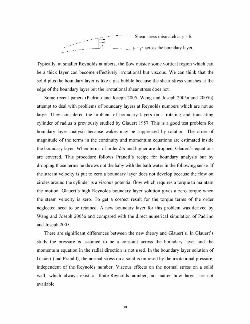
38

Shear stress mismatch at y = ��

p = piacross the boundary layer,

Typically, at smaller Reynolds numbers, the flow outside some vortical region which can

be a thick layer can become effectively irrotational but viscous. We can think that the

solid plus the boundary layer is like a gas bubble because the shear stress vanishes at the

edge of the boundary layer but the irrotational shear stress does not.

Some recent papers (Padrino and Joseph 2005, Wang and Joseph 2005a and 2005b)

attempt to deal with problems of boundary layers at Reynolds numbers which are not so

large. They considered the problem of boundary layers on a rotating and translating

cylinder of radius a previously studied by Glauert 1957. This is a good test problem for

boundary layer analysis because wakes may be suppressed by rotation. The order of

magnitude of the terms in the continuity and momentum equations are estimated inside

the boundary layer. When terms of order δ/a and higher are dropped, Glauert’s equations

are covered. This procedure follows Prandtl’s recipe for boundary analysis but by

dropping those terms he throws out the baby with the bath water in the following sense. If

the stream velocity is put to zero a boundary layer does not develop because the flow on

circles around the cylinder is a viscous potential flow which requires a torque to maintain

the motion. Glauert’s high Reynolds boundary layer solution gives a zero torque when

the steam velocity is zero. To get a correct result for the torque terms of the order

neglected need to be retained. A new boundary layer for this problem was derived by

Wang and Joseph 2005a and compared with the direct numerical simulation of Padrino

and Joseph 2005.

There are significant differences between the new theory and Glauert’s. In Glauert’s

study the pressure is assumed to be a constant across the boundary layer and the

momentum equation in the radial direction is not used. In the boundary layer solution of

Glauert (and Prandtl), the normal stress on a solid is imposed by the irrotational pressure,

independent of the Reynolds number. Viscous effects on the normal stress on a solid

wall, which always exist at finite-Reynolds number, no matter how large, are not

available.

39

In the new theory, the pressure is an unknown and the momentum equation in the

radial direction is needed. Since there is an extra unknown, an extra boundary condition

is needed and found in the requirement that the shear stress at the outer edge of the

boundary layer is continuous. Solutions in power series, like Glauerts, are obtained. The

inertia terms in the momentum equations give rise to the irrotational pressure and the

viscous terms lead to a viscous pressure which contributes to both lift and drag. The

solution is good to excellent agreement with the numerical solution when the boundary

layer thickness δ is properly chosen. The boundary layer is relatively thick and the

Reynolds numbers are not so large. The new solution is not self contained because δ is

not selected internally but is selected to fit data.

Acknowledgement: This work was supported in part by the National Science Foundation.

My collaborations with T. Funada and J.Wang on various topics mentioned in this essay

is most gratefully acknowledged.

References

Ackeret, J. Über exakte Lösungen der Stokes-Navier-Gleichungen inkompressibler

Flüssigkeiten bei veränderten Grenzbedingungen. Z. Angew. Math. Phys. 3, 259-270, 1952.

Basset, A. B. A Treatise on hydrodynamics, Deighton, Bell and Company 2 1888. Reprinted by Dover 1961

Batchelor, G. K. An introduction to fluid dynamics. Cambridge University Press, 1967. Bateman, H., 1932, See Dryden, Murnaghan, and Bateman, 1956. Bhaga, T. and Weber, M. Bubbles in viscous liquids: shapes, wakes and velocities. J.

Fluid Mech. 105, 61-85, 1981. Brabston, D. C. and Keller, H. B. Viscous flows past spherical gas bubbles. J. Fluid

Mech. 69, 179-189, 1975. Brown, R. A. S. The mechanics of large gas bubbles in tubes. Can. J. Chem. Engng. Q2,

217-223, 1965 Darwin, G. H. On the bodily tides of viscous and semi-elastic spheroids, Phil. Trans. cixx.

1, 1878. Davies, R. M. and Taylor, G. I. The mechanics of large bubbles rising through liquids in

tubes. Proc. R. Soc. Lond. A 200, 375-390, 1950. Dryden, H., Murnaghan, F. and Bateman, H. Hyrdrodynamics. Dover (a complete

unabridged reprinting of National Research Council Bulletin 84 1932 , 1956. Finzi, B., 1925, Sulla funzione di dissipazione di Lord Rayleigh, Atti Accad. Lincei, 6, 1:

215-220. .Funada, T., Joseph, D. D., Maehara, T. and Yamashita, S. Ellipsoidal model of the rise

of a Taylor bubble in a round tube, Int. J. Multiphase Flow, 31, 473-491, 2004.

40

Funada, T., Joseph, D. D. and Yamashita, S. Stability of a liquid jet into incompressible gases and liquids. Int. J. Multiphase Flow, 30, 1177-1208, 2004.

Funada, T., Saitoh, M.,Wang, J. and Joseph D. D. Stability of a liquid jet into incompressible gases and liquids: Part 2. Effects of the irrotational viscous pressure. To appear 2005

Funada, T., Joseph D. D., Yamashita, S., and Saitoh, M. Liquid jet into a high Mach number air stream. To appear 2005.

Funada, T., Wang, J. and Joseph, D. D. Purely irrotational theories of the effects of viscosity and viscoelastacity on capillary instability of a liquid cylinder. J. Non-Newtonian Fluid Mech., accepted, 2005.

Funada, T., Wang, J. and Joseph, D. D. Viscous potential flow analysis of stress induced cavitation in an aperture flow. Atomization and Sprays, accepted, 2005.

Glauert, H. The elements of aerofoil and airscrew theory. Cambridge University Press, 1943.

Hamel, G. Über die Potentialströmungen zäher Flüssigkeiten, Z. Angew. Math. Mech. 21, 129-139, 1941.

Harper, J. F. The motion of bubbles and drops through liquids. Adv. Appl. Mech. 12, 59-129, 1972.

Jeffreys, H. Equations of viscous fluid motion and the circulation theorem. Proc. Cambridge Phil. Soc., 24: 477-479, 1928.

Joseph, D. D. Bernoulli equation and the competition of elastic and inertial pressures in the potential flow of a second-order fluid. J.Non-Newtonian Fluid Mech., 42, 385-389, 1992.

Joseph, D. D. Viscous potential flow. J. Fluid Mech., 479, 191-197, 2003. Joseph, D. D. Rise velocity of a spherical cap bubble. J. Fluid Mech. 453, 109 – 132,

2003. Joseph, D. D., Belanger, J. and Beavers, G. S. Breakup of a liquid drop suddenly exposed

to a high-speed airstream. Int. J. Multiphase Flow, 25, 1263 – 1303, 1999. Joseph, D. D., Beavers, G. S. and Funada, T. Rayleigh-Taylor instability of viscoelastic

drops at high Weber numbers, J. Fluid Mech., 453, 109-132, 2002. Joseph, D. D. and Liao, T. Y. Potential Flow of Viscous and Viscoelastic Fluids. J. Fluid

Mech., 265, 1-23, 1994. Joseph, D. D. and Wang, J. The dissipation approximation and viscous potential flow. J.

Fluid Mech. 505, 365 – 377, 2004. Kang, I. S. and Leal, L. G. The drag coefficient for a spherical bubble in a uniform

streaming flow. Phys. Fluids 31, 233 – 237, 1988a. Kang, I. S. and Leal, L. G. Small-amplitude perturbations of shape for a nearly spherical

bubble in an inviscid straining flow (steady shapes and oscillatory motion). J. Fluid Mech. 187, 231 – 266, 1988b.

Lagrange, J. Mémoire sur la théorie du mouvement des fluides, Nouv. Mem. Acad. Berlin, 151-198 = Oeuvres 4, 695-748, 1781.

Lamb, H. Hydrodynamics, 6th edn. Cambridge University Press (Reprinted by Dover 1945), 1932.

.Levich, V. G. The motion of bubbles at high Reynolds numbers. Zh. Eksp. Teor. Fiz. 19, 18, 1949. Also in Physiochemical Hydrodynamics (English transl. By Scripta Technica), p. 436f. Prentice-Hall, 1962.

41

Lighthill, J. Waves in Fluids. Cambridge University Press, 1978. Longuet-Higgins, M. S. and Tanaka, M. On the crest instabilities of steep surface waves,

J. Fluid Mech. 336:51-68, 1997. Lundgren, T. S. and Mansour, N. N. Oscillations of drops in zero gravity with weak

viscous effects, J. Fluid Mech. 194, 479, 1988. .Miksis, M., Vanden-Broeck, J.-M. and Keller, J. B. Rising bubbles. J. Fluid Mech. 123, 31-41, 1982. Miller, C. A. and Scriven, L. E. The Oscillations of a Fluid Droplet Immersed in Another

Fluid. J. Fluid Mech. 32 (3), 417-435, 1968. Moore, D. W. The rise of gas bubble in a viscous liquid. J. Fluid Mech. 6, 113-130, 1959. Moore, D. W. The boundary layer on a spherical gas bubble. J. Fluid Mech. 16, 161 –

176, 1963. Moore, D. W. The velocity of rise of distorted gas bubbles in a liquid of small viscosity.

J. Fluid Mech. 23, 749–766, 1965. Navier, C. L. M. H. On the laws of motion of fluids taking into consideration the

adhesion of the molecules. Ann. Chim. Phys., 19: 234-245, 1822. Padrino, J. C. and Joseph, D. D. Numerical study of the steady state uniform flow past a

rotating cylinder, submitted, 2005. Padrino, J. C., Joseph, D. D., Funada, T. and Wang, J. Stress induced cavitation for the

streaming motion of a viscous liquid past a sphere. Submitted, 2005. Pipkin, A. C. Nonlinear phenomena in continua in nonlinear continuum theories in

mechanics and physics and their applications “Edizione Cremonese,” Roma, pp. 51-150, 1970. See also: Pipkin, A. C. and Tanner, R. in: Nemat-Nasser, S. (Ed.), A survey of theory and experiment in viscometric flows of viscoelastic liquid in mechanics today, Vol. 1, Pergamon, 1972.

Plesset, M. The dynamics of cavitation bubbles. ASME J. Appl. Mech. 16, 228-231, 1949. Poisson, S. D. Mémoire sur les equations générales de l’équilibre et du mouvement des

corps solides élastiques et des fluides, J. École Poly. 13, cahier 20, 1-174, 1829. Poritsky, M. The collapse on growth of a spherical bubble on cavity in a viscous fluid.

Proceedings of the first U.S. National Congress of Applied Mechanics held at the Illinois Institute of Technology, 813-821, ASME, 1951.

Prosperetti, A. Viscous effects on small-amplitude surface waves. Physics of Fluids. 19,

195-203, 1975. Prosperetti, A. Viscous effects on perturbed spherical flows. Quarterly J. Appl. Math. 35,

339-352, 1977 Romberg, G. Über die Dissipation in dichtebeständiger Strömung. Z. f. angew. Math. u.

Mech. 47, 155-162, 1967. Saffman, P. G. Vortex Dynamics. Cambridge Univ. Press, 1992. Saint-Venant, B. de. Note to be added to the memoir on the dynamics of fluids. Compt.

Rend., 17: 1240-1243, 1843. St. Venant, A.-J.-C.-B., de. Problème des mouvements que peuvent prendre les divers

points d’une masse liquide, ou solide ductile, continue dans un vase à parois verticales, pendant son écoulement par un orifice horizontal intérieur, C. R. Acad. Sci. Paris 68, 221-237, 1869.

42

Stokes, G. G. Considerations relative to the greatest height of oscillatory irrotational waves which can be propagated without change of form, Mathematical and physical papers, vol. I: 225-228, 1880.

Stokes, G. G. On the effect of the internal friction of fluids on the motion of pendulums, Trans. Cambr. Phil. Soc. 92, 8-106 = Papers 3, 1-141, 1850.

Stokes, Sir G. G. On the theories of the internal friction of fluids in motion. Trans. Cambridge Phil. Soc., 8: 287-319, 1845; Math. Phys. Papers. 1: 75-129.

Stokes, Sir G. G. Appendix B to Stokes 1847 on the highest irrotational oscillatory wave. Mathematical and physical papers, 5 vols. (Cambridge 1880-1905)

Tomotika, S. On the instability of a cylindrical thread of a viscous liquid surrounded by another viscous fluid, Proc. Roy. Soc. London A 150, 322–337, 1935.

Truesdell, C. A. Bernoulli’s theorem for viscous compressible fluids. Physical Review, 17, 535-536, 1950

Truesdell, C. A. The Kinematics of Vorticity. Indiana University Press, Indiana University Science Series, No. 19, 1954.

Wang, J. and Joseph, D. D. Pressure corrections for the effects of viscosity on the irrotational flow outside Prandtl's boundary layer, submitted, 2005a.

Wang, J. and Joseph, D. D. Boundary layer analysis for effects of viscosity of the irrotational flow on the flow induced by a rapidly rotating cylinder in a uniform stream, submitted, 2005b.

Wang, J. and Joseph, D. D. Purely irrotational theories of the effect of the viscosity on the decay of free gravity waves, submitted, 2005.

Wang, J., Joseph, D. D. and Funada, T. Pressure corrections for potential flow analysis of capillary instability of viscous fluids. J. Fluid Mech., 522, 383-394, 2005.

Wang, J., Joseph, D. D. and Funada, T. Viscous contributions to the pressure for potential flow analysis of capillary of two viscous fluids. Phys. Fluids, accepted, 2005.

Zierep, J. Viscous potential flow. Arch. Mech. 36, 127-133, Warszawa, 1984.

Potential Flow of Viscous Fluids: Historical Notes · Potential Flow of Viscous Fluids: Historical...

Documents

Transcript of Potential Flow of Viscous Fluids: Historical Notes · Potential Flow of Viscous Fluids: Historical...