Postglacial gravity change in Fennoscandia—three decades ...

Geophys. J. Int. (2019) 217, 1141–1156 doi: 10.1093/gji/ggz054Advance Access publication 2019 January 30GJI Gravity, geodesy and tides

Postglacial gravity change in Fennoscandia—three decades ofrepeated absolute gravity observations

Per-Anders Olsson,1 Kristian Breili,2,3 Vegard Ophaug,3 Holger Steffen,1

Mirjam Bilker-Koivula,4 Emil Nielsen,5 Tonis Oja,6 and Ludger Timmen7

1Geodetic Research Division, Lantmateriet, 801 82 Gavle, Sweden. E-mail: [email protected] Institute, Norwegian Mapping Authority, 3507 Hønefoss, Norway3Faculty of Science and Technology (RealTek), Norwegian University of Life Sciences (NMBU), 1433 As, Norway4Finnish Geospatial Research Institute, National Land Survey of Finland, 02430 Masala, Finland5National Space Institute, Technical University of Denmark (DTU Space), 2800 Kgs. Lyngby, Copenhagen, Denmark6Department of Geodesy, Estonian Land Board, 10621 Tallinn, Estonia7Institute of Geodesy, Leibniz Universitat Hannover (LUH), 30167 Hannover, Germany

Accepted 2019 January 29. Received 2019 January 23; in original form 2018 September 25

S U M M A R YFor the first time, we present a complete, processed compilation of all repeated absolute gravity(AG) observations in the Fennoscandian postglacial land uplift area and assess their ability toaccurately describe the secular gravity change, induced by glacial isostatic adjustment (GIA).The data set spans over more than three decades and consists of 688 separate observations at59 stations. Ten different organizations have contributed with measurements using 14 differentinstruments. The work was coordinated by the Nordic Geodetic Commission (NKG). Repre-sentatives from each country collected and processed data from their country, respectively, andall data were then merged to one data set. Instrumental biases are considered and presented interms of results from international comparisons of absolute gravimeters. From this data set,gravity rates of change (g) are estimated for all stations with more than two observations anda timespan larger than 2 yr. The observed rates are compared to predicted rates from a globalGIA model as well as the state of the art semi-empirical land uplift model for Fennoscandia,NKG2016LU. Linear relations between observed g and the land uplift, h (NKG2016LU) areestimated from the AG observations by means of weighted least squares adjustment as well asweighted orthogonal distance regression. The empirical relations are not significantly differ-ent from the modelled, geophysical relation g = 0.03 − 0.163(±0.016)h. We also present ag-model for the whole Fennoscandian land uplift region. At many stations, the observationalestimates of g still suffer from few observations and/or unmodelled environmental effects(e.g. local hydrology). We therefore argue that, at present, the best predictions of GIA-inducedgravity rate of change in Fennoscandia are achieved by means of the NKG2016LU land upliftmodel, together with the geophysical relation between g and h.

Key words: Geodetic instrumentation; Reference systems; Time variable gravity; Europe;Dynamics of lithosphere and mantle.

1 I N T RO D U C T I O N

Glacial isostatic adjustment (GIA) is the response of the Earthto changing loads on its surface due to build-up and ablation ofice sheets and glaciers. The response includes changes in shape(deformation), gravity potential, stress and rotation of the Earth(Wu & Peltier 1982). The effects of GIA that are presently observedresult from several glaciations with ice sheets covering large partsof, for example, North America, Northern Europe and Patagonia.

The last glaciation peaked about 22 000 yr ago in Fennoscandia(Lambeck et al. 2010). Although the ice vanished about 10 000 yrago (Lambeck et al. 2010), the Earth is still readjusting due tothe viscoelastic nature of the mantle, which leads to time-delayedprocesses. In Fennoscandia, this is visible in the ongoing surfaceuplift that peaks at about 1 cm yr−1 near the Swedish coast to theGulf of Bothnia (Steffen & Wu 2011; Fig. 1).

The GIA process in Fennoscandia is well known and extensivelystudied. Ekman (1991) describes the early history of research within

C© The Author(s) 2019. Published by Oxford University Press on behalf of The Royal Astronomical Society. This is an Open Accessarticle distributed under the terms of the Creative Commons Attribution License (http://creativecommons.org/licenses/by/4.0/), whichpermits unrestricted reuse, distribution, and reproduction in any medium, provided the original work is properly cited. 1141

Dow

nloaded from https://academ

ic.oup.com/gji/article-abstract/217/2/1141/5304614 by guest on 18 M

arch 2019

mailto:[email protected]

http://creativecommons.org/licenses/by/4.0/

1142 P.-A. Olsson et al.

10˚

10˚

20˚

20˚

30˚

30˚

55˚55˚

60˚ 60˚

65˚ 65˚

70˚ 70˚

10˚

10˚

20˚

20˚

30˚

30˚

55˚55˚

60˚ 60˚

65˚ 65˚

70˚ 70˚

0

0

2

2

4

4

6

6

8

8

10

10

HELSSMID

SULD

TRDHVVOL

SUUR

TORAKURE

METS

SODA

VAAAVAAB

JOEN

KEVO

KUUB

ANDO

BODABODB

HAMM

HONN

HONAHONB

HONCJON2

KAUT

KOL1KOL2

STVA

TROM

TRDA

TRYBTRYC

VAGA

VEGA

ALES

NMBU

ARJE

BORA

GAVL

KIRU

KRAM

LYCK

MARAMARB

ONSAONSC

ONSNONSS

OSTERATA

SKEL

SMOG

VISB

VLNS

KLPD PNVZ

POPERIGA

VISK

Figure 1. Stations with repeated gravity observations in Fennoscandia.Blue dots represent absolute gravity stations and red dots (and lines) theFennoscandian land uplift gravity lines with relative observations. Isolinesshow the vertical displacement rate according to the semi-empirical landuplift model NKG2016LU abs (mm yr−1).

this field and Steffen & Wu (2011) review modern observational andmodelling efforts in this region.

One important observable of GIA, but less used and investigatedcompared to deformation, is the secular gravity change. Redistri-bution of masses within the Earth as well as on the surface causechanges in the gravity field. Also the vertical land motion/upliftitself induces changes in gravity on the surface of the Earth. Knowl-edge about this GIA-induced rate of change of gravity, g, is impor-tant in many aspects, for example

(1) for reduction of terrestrial gravity observations to a certainepoch,

(2) as ground truth for satellite gravity missions (e.g. Steffenet al. 2009; Muller et al. 2012), and

(3) for constraining and tuning GIA models (e.g. Steffen et al.2014; Van Camp et al. 2017).

Several models of the GIA-induced vertical displacement ratehave been published for Fennoscandia (e.g. Ekman 1996; Lambecket al. 1998; Milne et al. 2004; Agren & Svensson 2007; Lidberget al. 2010). Although several observational g-results exist (seeTable 1), no g-model for Fennoscandia has been published so far.This is primarily because terrestrial gravity measurements are timeconsuming and need on-site manpower. Absolute gravity (AG) ob-servations are consequently more expensive than most other geode-tic observations. In addition, combination of gravity measurementsis challenging due to sensor-affecting incidents and local gravityeffects that may mask the secular trend due to GIA.

The first systematic observations of the GIA-induced gravitychange were repeated relative gravity observations along the so-called Fennoscandian land uplift gravity lines. They consist of foureast-west high precision relative gravity profiles, approximately fol-lowing the latitudes 65◦, 63◦, 61◦ and 56◦ (see Fig. 1). Measurements

along the Finnish part of the 63◦ line started in 1966 followed bythe rest of the lines from the mid-1970s (Kiviniemi 1974; Ekman &Makinen 1996; Makinen et al. 2005). The work with the Fennoscan-dian land uplift gravity lines was initiated and coordinated by theNordic Geodetic Commission (NKG).

From the late 1980s the relative gravity observations along theuplift lines have been complemented and gradually succeeded byrepeated AG observations. In 1988, the Finnish Geodetic Institute(FGI) started this work using a free-fall absolute gravimeter JILAg-type (Torge et al. 1987), JILAg#5. This gravimeter was mainly usedin Finland but also at some stations in the other Scandinavian andespecially the Baltic countries. During the 1990s, the JILAg mea-surements were complemented by observations with its successor,the FG5 (Niebauer et al. 1995). These first FG5 campaigns wereperformed by the National Oceanic and Atmospheric Administra-tion (NOAA), USA, in 1993 and 1995. Further FG5 campaigns wereconducted by the Bundesamt fur Kartographie und Geodasie (BKG)in 1993, 1995, 1998 and 2003 on 15 stations distributed in the up-lift area. In 2003–2008 comprehensive campaigning was carriedout with an FG5 instrument by the Leibniz Universitat Hannover(LUH), Germany. During that time also the FGI, the NorwegianUniversity of Life Sciences (NMBU) and Lantmateriet (the Swedishmapping, cadastral and land registration authority) invested in FG5gravimeters and started with repeated AG observations. In 2008 theTechnical University of Denmark (DTU) started making repeatedmeasurements with their A10 absolute gravimeter (Micro-g La-Coste 2008). Today there are 688 AG observations on 59 stations inthe region (Fig. 1), most of them co-located with Global NavigationSatellite Systems (GNSS) reference stations. Two of the stations,Metsahovi (since 1994; Virtanen 2006) and Onsala (since 2008),also house superconducting gravimeters (SG). As in the case of theland uplift lines, the work with absolute observations was and iscoordinated by the NKG.

Only parts of the Fennoscandian repeated AG observations havehitherto been published. Gitlein (2009) published the results fromthe BKG, NOAA and LUH campaigns in 1993–2008 with focuson the LUH data. Ophaug et al. (2016) published all FG5 data onthe Norwegian stations. Selected observations have been includedin special studies, for example, to address the g/h ratio (Pettersen2011). Table 1 gives an overview of publications addressing dif-ferent parts of the whole data set. This includes some unpublishedreports and poster presentations since they, in the absence of betterreferences, sometimes have been cited in the literature.

Besides Fennoscandia, GIA-induced surface deformation andgravity changes can also be observed in North America. Comparedto Fennoscandia, both the signal strength and the geographical ex-tent are larger. AG time-series from North America was analysedby, for example, Larson & van Dam (2000) and Lambert et al.(2001, 2006, 2013a,b). A map of gravity rate of change in NorthAmerica, but mainly based on relative gravity measurements, waspublished by Pagiatakis & Salib (2003). In their study, they re-adjusted the primary Canadian Gravity Standardization Networkusing relative gravity measurements spanning over 40 yr. The grav-ity rate of change was introduced as an unknown in the observationequation and AG measurements were used as weighted constraintsin the (least squares) adjustment.

The relation between g and the vertical displacement rate of thecrust, h, is also an important observable since it

(1) is affected by both the vertical movement itself as well as bymass changes beneath the surface and therefore contains informa-tion on the underlying geophysics and geodynamics (e.g. Ekman &Makinen 1996; de Linage et al. 2009),

Dow



arch 2019

Postglacial gravity change in Fennoscandia 1143

Table 1. Overview of important publications and reports on repeated AG observations in Fennoscandia.

Reference Data set Comment

Roland (1998) 1991–1995. Observations at 23 stations in Finland, Norwayand Sweden

Technical report NMA (in Norwegian)

Engfeldt et al. (2006) 2003–2005. g at 14 stations in Finland, Norway and Sweden.Only FG5

Poster

Makinen et al. (2006) 1976–2006. g at Finnish stations PosterBilker-Koivula et al. (2008) 1976–2007. Observations at six Finnish stationsGitlein (2009) 1993–2008. Observations at 37 stations in the Scandinavian

and Baltic countries. Only NOAA, BKG and LUHPhD thesis

Steffen et al. (2009) 2004–2007. Six stations. Only LUH Ground truth for GRACEBreili et al. (2010) g at Norwegian stations from observations with FG5#226Makinen et al. (2010) 1988–2009. g at 23 stations in the Scandinavian and Baltic

countriesPoster

Pettersen (2011) From Engfeldt et al. (2006) Address the g/h-ratioTimmen et al. (2012) 2004–2008. From Gitlein (2009). Only LUH g/h=0.163Muller et al. (2012) Same as Timmen et al. (2012) Ground truth for GRACENordman et al. (2014) Timmen et al. (2012), Pettersen (2011), and Breili et al. (2010) Compare g and h from different sourcesTimmen et al. (2015) 2003–2014. Only Onsala. Only FG5#220 and FG5#233 Evaluate gOphaug et al. (2016) 1993–2014. Only Norwegian stations

(2) is used for evaluation of global Terrestrial Reference Frames(e.g. Mazzotti et al. 2011; Collilieux et al. 2014) and

(3) is used for separating the GIA signal from present-day icemelting signals in Greenland and Antarctica (e.g. Wahr et al. 1995;van Dam et al. 2017).

In addition, a trustworthy relation between g and h also allowsus to make transformations between, and combine, the two observ-ables.

As mentioned, in regions like Antarctica and Greenland, the ratiobetween g and h has been used for separating the present-day ice-mass change signal from the GIA signal, the latter induced byhistorical ice mass variations (Wahr et al. 1995; James & Ivins1998; Fang & Hager 2001; Purcell et al. 2011; Memin et al. 2012).From an analytical study with a GIA model for Greenland andAntarctica, Wahr et al. (1995) found the viscous part of the ratioto be ∼−0.154 μGal mm−1. Using the ice model ICE-3G, James &Ivins (1998) predicted g and h for Antarctica, and found their ratio tobe ∼−0.16 μGal mm−1. These predictions are based on modellingand are difficult to verify by observations, because gravity changedue to present-day ice mass variation is superimposed by the viscousgravity signal.

In North America and Fennoscandia the situation is different.Here, the signal is strongly dominated by the past GIA signal andthe ice-free conditions make it possible to conduct repeated mea-surements of both gravity and height changes. Table 2 summarizespublished ratios based on observations in these regions.

Olsson et al. (2015) investigated the geophysical relation betweeng and h in previously glaciated areas (like Fennoscandia and Lauren-tia) using a GIA model, similar to the one described in Section 2.5,and found that

(1) their ratio varies in the spectral domain and is smaller (lessnegative) in the lower part of the spectrum, implying that for aregion where the GIA signal is smooth and has a large geographicalextent (Laurentia) the ratio is expected to be smaller than for aregion where higher degrees of the spectrum dominate the signal(Fennoscandia),

(2) the borderline between the uplift area and the forebulge area(zero line) for g and h does not exactly coincide, which affects theirratio especially where the signal is small,

(3) within Fennoscandia the ratio varies laterally in such a waythat for practical applications these variations can be neglected,

(4) local effects, such as direct attraction and short wavelengthelastic deformation from present-day GIA-induced sea level varia-tions do not significantly affect the ratio other than in extreme cases(when the station in question is located very close to and high abovethe sea).

These conclusions imply that for Fennoscandia it is a reasonableassumption to estimate a single linear relation between g and h forthe entire region.

For the first time we present estimated gravity rates of changebased on all repeated gravity observations, spanning over threedecades, in the Fennoscandian land uplift area. All observations areprovided and described in detail. Estimated g values are assessedby the geophysical relation between g and h, found from GIA-modelling, and the uncertainties in these relations are discussed. Wealso suggest a g model covering the whole area, based on the stateof the art land uplift model and the geophysical relation between gand h.

In Section 2, we describe the AG data set, how data from differentsources have been processed and merged, known error sources, anduncertainty estimates. We also introduce land uplift data sets and ageophysical GIA model for comparison to our observational gravityrate of change. In Section 3, we estimate observational values ofg and compare it with a semi-empirical land uplift model as wellas a pure GIA model. The relation between g and h is estimatedand studied in Section 4 and it is further used for constructing ag-model, covering the whole area. This is followed by a discussionof the results and a summary of conclusions. Detailed informationabout the stations and all observations are provided as SupportingInformation (Tables S2 and S4).

2 DATA A N D M O D E L S

2.1 The AG stations

We have used data from 59 stations in the region where repeatedAG observations have been conducted (Fig. 1 and Table S2). Stef-fen et al. (2012) studied optimal locations for AG observations andconcluded that, except for the northwestern part of Russia, these

Dow



arch 2019


Table 2. Published observations of g/h in previously glaciated areas (from Olsson et al. 2015).

Area g/h Note References(μGal mm−1)

Fennoscandia −0.204 ± 0.058 Relative gravity observations every 5th yr; time span ∼27 yr. h frommareographs and levelling

Ekman & Makinen (1996)

Fennoscandia −0.16 ± 0.05 to−0.18 ± 0.06

Ekman & Makinen (1996) revisited, this time with more observations of g aswell as h (including GNSS)

Makinen et al. (2005)

Fennoscandia −0.163 ± 0.02 Four years of annual AG-observations on eight stations. h from GNSS(Lidberg et al. 2007). For the different stations, the ratios vary between−0.114 ± 0.031 and −0.232 ± 0.059 μGal mm−1

Timmen et al. (2012)

Fennoscandia −0.17 to −0.22 13 stations with repeated AG observations compared to vertical rates derivedfrom tide-gauge data and GNSS data

Pettersen (2011)

Laurentia ∼−0.154 Four stations of co-located GNSS and AG. Total time span 6 yr. The ratio−0.154 μGal mm−1 is within the error bars of these observations

Larson & van Dam (2000)

Laurentia −0.18 ± 0.03 Four stations of co-located GNSS and AG. Three of the stations are the sameas in Larson & van Dam (2000)

Lambert et al. (2006)

Laurentia −0.17 ± 0.01 Eight AG stations whereof six are co-located with GNSS including the fourstations in Lambert et al. (2006). Time spans 7–21 yr

Mazzotti et al. (2011)

Alaska −0.21 ± 0.09 and−0.18 ± 0.05

The viscous part of the ratio in an area affected by present-day ice masschange. Different ratios depending on how the present-day signal is correctedfor

Sato et al. (2012)

stations form a complete and adequate network for providing con-straints for the study of GIA parameters.

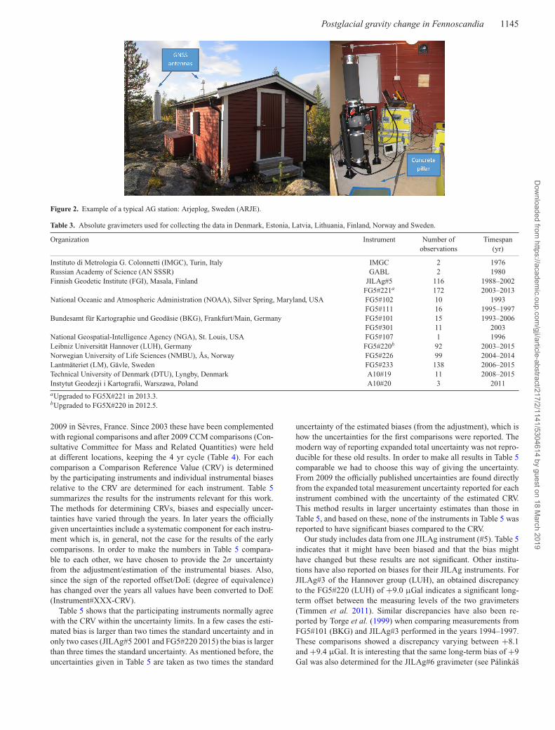
Most of the stations are co-located with permanent GNSS ref-erence stations in the so-called BIFROST (Baseline Inference forFennoscandian Rebound Observations, Sea level and Tectonics) net-work (see e.g. Johansson et al. 2002; Lidberg et al. 2010). Many ofthese stations have GNSS time-series spanning more than 20 yr. TheAG stations typically consist of a concrete pillar mounted directlyon solid bedrock, housed in the same building as the GNSS station(Fig. 2). Some of the stations (e.g. Metsahovi, Martsbo, Onsala andTrysil) have two or more pillars and are therefore suitable for com-parisons of instruments by means of simultaneous observations.Some stations are not dedicated AG stations but rather housed inpublic, stable buildings.

Metsahovi (MET) and Onsala (ONS) are geodetic fundamentalstations in the sense that they host instrumentation for a large varietyof observational techniques like AG, superconducting gravity, verylong baseline interferometry, satellite laser ranging (MET), tidegauge (ONS) and monitoring of local hydrology.

In addition to the stations discussed above, some hundred otherAG stations have also been observed with absolute gravimeters(typically A10 gravimeters). These are more simple stations likea benchmark mounted in a rock, stairs or similar. The purposeof these observations was not to study GIA or other geophysicalprocesses and phenomena but rather to serve as datum points fornational gravity reference systems. These stations and observationsare therefore not treated here.

2.2 The AG observations

During the time period 1988–2015, 688 repeated AG observationswere conducted at the stations described above. One observationis here understood to be the mean of a large number of free fallexperiments (drops). The drops are normally executed during atime period of ∼12–48 hr and grouped in sets of ∼50–100 drops.If there was more than one consecutive set-up of the instrument(e.g. with different orientations) at one visit of the station, then theresults of the different set-ups are merged to one observation.

Many different organizations have contributed with observations(Table 3). Each organization initially processed their own data. One

representative for each country (Table S1) then collected, and insome cases reprocessed, all data from stations in his/her country,respectively. Data from all participating countries have then beenmerged into one database (Table S4).

The bulk of the observations was collected using FG5 gravime-ters (Niebauer et al. 1995). These data were processed using the‘g’ software (Micro-g LaCoste 2012) with final International EarthRotation and Reference System Service (IERS) polar coordinates,calibrated rubidium frequencies, and standard modelling of grav-itational effects due to earth tides, ocean loading and varying at-mospheric pressure, as implemented in the ‘g’ software [for detailsconcerning e.g. ocean tide loading (OTL) models, see SupportingInformation]. There have been attempts to perform a refined mod-elling of the gravitational effect due to ocean loading, non-tidalocean loading and global hydrology (Ophaug et al. 2016), as wellas the atmosphere (Gitlein 2009; Ophaug et al. 2016). The generalconclusions of these studies are that refined modelling does not giveany significant improvement with respect to the gravity trends onaverage. In addition, the lack of corrections for local hydrology,which could dominate the gravity rate at a specific site, is identifiedas an important issue for further research (see e.g. Van Camp et al.2016b). Thus, until the refined modelling improves and the effectof local hydrology can be embedded, we stick with the standardprocessing scheme in this work.

Apart from FG5 also IMGC (Germak et al. 2006), GABL (Ar-nautov et al. 1983), JILAg (Niebauer et al. 1986) and A10 (Micro-gLaCoste 2008) absolute gravimeters were used (see Table 3).

All data are presented in the zero tide system. Some of the firstobservations (e.g. IMGC from 1976) were originally in the mean tidesystem but have been reprocessed to the zero tide system (Haller &Ekman 1988), following the IAG resolution from 1983 (IAG 1984).

Details about the data and data processing are given in the Sup-porting Information.

2.3 Instrumental biases

AG observations are in general sensitive to instrumental biases (oroffsets). In order to detect such biases the International Bureauof Weights and Measures (BIPM) organized international compar-isons of absolute gravimeters on a regular basis between 1981 and

Dow



arch 2019


Figure 2. Example of a typical AG station: Arjeplog, Sweden (ARJE).

Table 3. Absolute gravimeters used for collecting the data in Denmark, Estonia, Latvia, Lithuania, Finland, Norway and Sweden.

Organization Instrument Number of Timespanobservations (yr)

Instituto di Metrologia G. Colonnetti (IMGC), Turin, Italy IMGC 2 1976Russian Academy of Science (AN SSSR) GABL 2 1980Finnish Geodetic Institute (FGI), Masala, Finland JILAg#5 116 1988–2002

FG5#221a 172 2003–2013National Oceanic and Atmospheric Administration (NOAA), Silver Spring, Maryland, USA FG5#102 10 1993

FG5#111 16 1995–1997Bundesamt fur Kartographie und Geodasie (BKG), Frankfurt/Main, Germany FG5#101 15 1993–2006

FG5#301 11 2003National Geospatial-Intelligence Agency (NGA), St. Louis, USA FG5#107 1 1996Leibniz Universitat Hannover (LUH), Germany FG5#220b 92 2003–2015Norwegian University of Life Sciences (NMBU), As, Norway FG5#226 99 2004–2014Lantmateriet (LM), Gavle, Sweden FG5#233 138 2006–2015Technical University of Denmark (DTU), Lyngby, Denmark A10#19 11 2008–2015Instytut Geodezji i Kartografii, Warszawa, Poland A10#20 3 2011aUpgraded to FG5X#221 in 2013.3.bUpgraded to FG5X#220 in 2012.5.

2009 in Sevres, France. Since 2003 these have been complementedwith regional comparisons and after 2009 CCM comparisons (Con-sultative Committee for Mass and Related Quantities) were heldat different locations, keeping the 4 yr cycle (Table 4). For eachcomparison a Comparison Reference Value (CRV) is determinedby the participating instruments and individual instrumental biasesrelative to the CRV are determined for each instrument. Table 5summarizes the results for the instruments relevant for this work.The methods for determining CRVs, biases and especially uncer-tainties have varied through the years. In later years the officiallygiven uncertainties include a systematic component for each instru-ment which is, in general, not the case for the results of the earlycomparisons. In order to make the numbers in Table 5 compara-ble to each other, we have chosen to provide the 2σ uncertaintyfrom the adjustment/estimation of the instrumental biases. Also,since the sign of the reported offset/DoE (degree of equivalence)has changed over the years all values have been converted to DoE(Instrument#XXX-CRV).

Table 5 shows that the participating instruments normally agreewith the CRV within the uncertainty limits. In a few cases the esti-mated bias is larger than two times the standard uncertainty and inonly two cases (JILAg#5 2001 and FG5#220 2015) the bias is largerthan three times the standard uncertainty. As mentioned before, theuncertainties given in Table 5 are taken as two times the standard

uncertainty of the estimated biases (from the adjustment), which ishow the uncertainties for the first comparisons were reported. Themodern way of reporting expanded total uncertainty was not repro-ducible for these old results. In order to make all results in Table 5comparable we had to choose this way of giving the uncertainty.From 2009 the officially published uncertainties are found directlyfrom the expanded total measurement uncertainty reported for eachinstrument combined with the uncertainty of the estimated CRV.This method results in larger uncertainty estimates than those inTable 5, and based on these, none of the instruments in Table 5 wasreported to have significant biases compared to the CRV.

Our study includes data from one JILAg instrument (#5). Table 5indicates that it might have been biased and that the bias mighthave changed but these results are not significant. Other institu-tions have also reported on biases for their JILAg instruments. ForJILAg#3 of the Hannover group (LUH), an obtained discrepancyto the FG5#220 (LUH) of +9.0 μGal indicates a significant long-term offset between the measuring levels of the two gravimeters(Timmen et al. 2011). Similar discrepancies have also been re-ported by Torge et al. (1999) when comparing measurements fromFG5#101 (BKG) and JILAg#3 performed in the years 1994–1997.These comparisons showed a discrepancy varying between +8.1and +9.4 μGal. It is interesting that the same long-term bias of +9Gal was also determined for the JILAg#6 gravimeter (see Palinkas

Dow



arch 2019


Table 4. Overview of official international (ICAG), European (ECAG) and regional (EURAMET) Comparisons ofabsolute gravimeters, held in Sevres (France) until the year 2015, Walferdange and Belval (Luxembourg). The standarddeviations (1σ ) of all participating instruments’ degrees of equivalences (DoEs) are also given for each campaign.

Comparison Location Approximate σ of DoEs Referenceepoch (μGal)

ICAG 81-82 Sevres 1982.0 ∼8 Boulanger et al. (1983)ICAG 1985 Sevres 1985.5 4.4 Boulanger et al. (1986)ICAG 1989 Sevres 1989.5 7.6 Boulanger et al. (1991)ICAG 1994 Sevres 1994.4 3.3 Marson et al. (1995)ICAG 1997 Sevres 1997.9 2.8 Robertsson et al. (2001)ICAG 2001 Sevres 2001.6 5.5 Vitushkin et al. (2002)ECAG 2003 Walferdange 2003.8 1.9 Francis & van Dam (2006)ICAG 2005 Sevres 2005.7 3.7 Jiang et al. (2011)ECAG 2007 Walferdange 2007.9 2.1 Francis et al. (2010)ICAG 2009 Sevres 2009.8 4.2 Jiang et al. (2012)ECAG 2011 Walferdange 2011.9 3.1 Francis et al. (2013)ICAG 2013 Walferdange 2013.9 3.8 Francis et al. (2015)EURAMET 2015 Belval 2015.8 5.1 Palinkas et al. (2017)

Table 5. Official results from the international comparisons in Table 4. The numbers correspond to the degree of equivalence (DoE), that is the estimated biasof each instrument, compared to comparison reference values, and the associated expanded uncertainty (∼95% confidence level (2 σ )). Only results relevantfor this work are presented.

IMGC GABL JILAg#5 FG5#101 FG5#102 FG5#111 FG5#107

ICAG 81-82 −6 7ICAG 1985ICAG 1989 −8.1 ± 6.6ICAG 1994 −3.9 ± 8 −0.5 ± 6.4 −2.1 ± 6 1.7 ± 6ICAG 1997 0.5 ± 7.2 −2.7 2.5 ± 6.0ICAG 2001 5.7 ± 3.2 2.9 ± 8.0ECAG 2003ICAG 2005 −2.5 ± 3.0ECAG 2007 2.2 ± 1.8

FG5#301 FG5#220 FG5#221 FG5#226 FG5#233 A10#19 A10#20ICAG 2001 −4.5 ± 5.6ECAG 2003 −1.3 ± 2.0 −1.8 ± 2.8 0.9 ± 3.8ICAG 2005 −0.5 ± 3.6ECAG 2007 2.5 ± 2.2 0.1 ± 2.2 −3.4 ± 2.4 1.0 ± 1.8ICAG 2009 1.7 ± 2.8 1.6 ± 3.2 1.0 ± 2.8 5.0 ± 12.2ECAG 2011 1.8 ± 3.2 0.0 ± 3.6 4.7 ± 3.3 −5.1 ± 11.7ICAG 2013 2.3 ± 3.11 1.5 ± 3.3a 2.2 ± 3.4 −4.6 ± 6.5EURAMET 2015 5.2 ± 2.91 −2.1 ± 3.31 2.5 ± 3.4 −5.3 ± 7.5aUpgraded to FG5X.

et al. 2012). For the Canadian gravimeter JILAg#2 a systematicoffset of +4.1 μGal has been found in Liard et al. (2003). Somehints are given in Wilmes et al. (2003) that similar offsets may ex-ist in other JILA gravimeters with respect to FG5 meters. Besidesthese long-term biases, varying biases valid for shorter periods mayexists for gravimeters and depend on the experts who re-adjust theinstruments from time to time.

One major disadvantage of the JILAg design compared withthe FG5 instruments is the high sensitivity of JILAg meters tofloor tilts occurring during each drop which is triggered by thedropping mechanism similar in all drops of a measuring set. Becausethe interferometer design is not following the Abbe rule like it isrealized in the FG5 instruments (reference and test prism in onevertical line), tilt coupling errors of some microgal could occur atlocations with weak floor conditions. That introduces a systematicerror in the station determination by the gravimeter and can onlybe detected by a new set-up of the meter with another orientation.For FG5 gravimeters, the effect has been minimized, see Niebaueret al. (1995).

By assessing local comparisons between some of the instrumentsrelevant for this study also Pettersen et al. (2010) conclude that datafrom these instruments reveal no systematic biases, but occasionalshifts from 1 yr to another are noted. This was also found by Ols-son et al. (2016). They showed that time-series from the FG5#233gravimeter indicated a jump in 2010. The jump occurred duringa service of the instrument by the manufacturer, but no real ex-planation has been found, yet. The effects of that jump could bereduced by introducing a small correction based on the results fromthe international comparisons.

Based on the results above, data from FG5#233 have beencorrected for the suspected jump in this study (see further Section 3)but no other biases between instruments have been considered.

2.4 The NKG2016LU land uplift model

NKG2016LU is a successor of the empirical land uplift modelNKG2005LU, which has been the official standard model for geode-tic land uplift applications in the Nordic countries for the last decade.

Dow



arch 2019


Figure 3. Uncertainty of g predicted using the land uplift model NKG2016LU abs together with a geophysical relation between g and h.

NKG2005LU was released by the NKG Working Group for HeightDetermination in 2006. Empirical here means that it heavily relieson geodetic observations such as repeated levelling and time-seriesfrom tide gauges and GNSS stations. The different types of obser-vations are combined by means of least squares collocation. Forinterpolation (and extrapolation) between the observation points, ageophysical GIA model by Lambeck et al. (1998) was used. Fora thorough description of NKG2005LU, see Agren & Svensson(2007) and Vestøl (2007).

In 2016, the NKG Working Group on Geoid and Height Sys-tems released the land uplift model NKG2016LU, which is nowcalled semi-empirical in order to emphasize that it, in addition toobservations, also includes a GIA modelling component. Notabledifferences to NKG2005LU include

(1) longer GNSS time-series. Vertical velocities from theBIFROST 2015/16 calculation, processed in GAMIT/GLOBK andfinalized in 2016 March 1. This is an updated version of Kierulfet al. (2014).

(2) omission of tide gauge data. Spatial and especially temporalvariations in the rate of change of mean sea level (e.g. acceleratingsea level rise during the last decades) prompted the decision not toinclude tide gauge data in NKG2016LU.

(3) more thorough GIA modelling, better adapted to geodeticobservations in Fennoscandia (Steffen et al. 2016).

NKG2016LU comes in two versions, NKG2016LU lev andNKG2016LU abs. NKG2016LU lev is the land uplift as mea-sured with repeated levelling, that is relative to the geoid.NKG2016LU abs (see Fig. 1) is the absolute land uplift inITRF2008 as observed by GNSS. In the observation points, the

mean difference between the BIFROST GNSS solution and the fi-nal NKG2016LU abs model is 0.02 ± 0.42 (1σ ) mm yr−1, whichcorresponds to ∼−0.003 ± 0.07 (1σ ) μGal yr−1 (see below). AsNKG2016LU is given in the same reference frame as the BIFROSTGNSS solution, but also includes levelling data, and gives a trust-worthy interpolation between the observation points (and thus avalue for all gravity points and any other point), we take it ratherthan the GNSS solution itself as a reference model.

For conversion of the NKG2016LU abs land uplift to gravityrate of change we use the factor C = −0.163 μGal mm from−1 themodelled linear relation

g = 0.03 − 0.163h, (1)

found by Olsson et al. (2015), valid for 1-D geophysical GIA models(normal mode approach) in Fennoscandia. The uncertainty of thefactor has been estimated to u(C) ∼ ±0.016 μGal mm−1 (Ophauget al. 2016).

Assuming an internal uncertainty of 0.2 mm yr−1 inNKG2016LU abs (Jonas Agren, personal communication, 2016)and uncertainties in the drift of the origin relative to the Earth’scentre of mass and in the scale of ITRF2008 of 0.5 and 0.3 mmyr−1, respectively (Collilieux et al. 2014), we estimate the total un-certainty of NKG2016LU abs to u(h) ∼ 0.6164 mm yr−1 by errorpropagation. Then the uncertainty of the predicted gravity change is

u(gLU) =√

u(C)2h2 + u(h)2C2 =√

0.0162h2 + 0.010 μGal yr−1

where gLU = C · hN K G2016LU abs . In Fennoscandia 0.1 ≤ u(gLU) <

0.2 (μGal yr−1) (see Fig. 3).

Dow



arch 2019


Table 6. Absolute land uplift rate, h (mm yr−1) and gravity rate of change, g (μGal yr−1). Subscript GNSS referes to the BIFROST 2015/16 solution, GIA tothe geophysical GIA model, LU means -0.163·NKG2016LU abs and I and II are estimates based on the corresponding data sets (see text). ε are the standardizedresiduals from the estimations of g/h trend lines (eq. 4). The last two columns show the total number of AG observations (corresponding to Dataset I) at eachstation and their time span [years].

Stn hLU hG N SS gG I A gLU gI εI gI I εI I nobs �T

ALES 1.63 1.73 −0.05 −0.27 ± 0.10 −0.29 ± 0.48 −0.2 −0.29 ± 0.36 −0.3 5 7.0ANDO 1.69 1.26 0.09 −0.28 ± 0.10 −1.09 ± 0.55 −1.6 −1.09 ± 0.41 −2.2 5 6.0ARJE 8.15 7.97 −1.02 −1.33 ± 0.16 −0.74 ± 0.31 1.9 −1.09 ± 0.23 1.1 11 10.0BODA 3.94 −0.35 −0.64 ± 0.12 −2.23 ± 0.72 −2.3 4 5.1BODB 3.96 3.88 −0.35 −0.65 ± 0.12 −1.06 ± 0.83 −0.5 4 4.0BORA 3.52 3.58 −0.40 −0.57 ± 0.11 0.02 ± 0.34 1.7 4 11.0GAVL 7.69 −1.07 −1.25 ± 0.16 −1.03 ± 0.18 1.2 −1.26 ± 0.15 −0.0 44 8.9HELS 1.41 −0.06 −0.23 ± 0.10 1.24 ± 0.92 1.6 5 11.5HONB 5.04 −0.80 −0.82 ± 0.13 −0.92 ± 0.21 −0.6 4 16.7HONC 4.94 5.14 −0.78 −0.81 ± 0.13 −0.07 ± 0.21 3.3 12 15.9HONN 2.54 2.36 −0.29 −0.41 ± 0.11 −0.38 ± 0.72 −0.0 5 4.9JOEN 3.91 3.43 −0.66 −0.64 ± 0.12 −0.56 ± 0.28 0.0 −0.44 ± 0.22 0.7 9 12.7KAUT 5.27 5.11 −0.72 −0.86 ± 0.13 −2.18 ± 0.67 −2.0 5 4.9KEVO 4.19 4.34 −0.53 −0.68 ± 0.12 0.21 ± 0.46 1.8 6 6.0KIRU 6.95 7.08 −0.94 −1.13 ± 0.15 −0.92 ± 0.17 1.1 −1.13 ± 0.13 0.0 14 20.0KRAM 9.83 9.75 −1.33 −1.60 ± 0.19 −1.45 ± 0.33 0.4 −1.80 ± 0.25 −0.7 10 10.0KUUB 7.09 7.29 −1.11 −1.16 ± 0.15 −1.28 ± 0.53 −0.0 4 6.1LYCK 9.95 −1.29 −1.62 ± 0.19 −1.63 ± 0.44 0.0 −1.90 ± 0.33 −0.7 6 8.0MARA 7.58 7.59 −1.05 −1.24 ± 0.16 −1.04 ± 0.12 1.4 −1.29 ± 0.10 −0.5 36 38.5METS 4.49 4.29 −0.35 −0.73 ± 0.12 −0.75 ± 0.05 −1.0 223 32.4NMBU 4.73 −0.79 −0.77 ± 0.13 −0.56 ± 0.28 0.7 −0.56 ± 0.21 0.8 10 9.8ONSA 2.89 2.90 −0.26 −0.47 ± 0.11 −0.16 ± 0.09 3.0 −0.30 ± 0.07 1.6 52 21.8OSTE 8.56 8.64 −1.10 −1.40 ± 0.17 −1.00 ± 0.27 1.4 −1.30 ± 0.20 0.6 13 12.0RATA 10.17 10.02 −1.39 −1.66 ± 0.19 −1.74 ± 0.44 −0.2 −2.01 ± 0.33 −0.9 6 8.0RIGA 0.85 1.24 −0.08 −0.14 ± 0.10 −0.68 ± 0.21 −2.8 5 18.1SKEL 10.12 10.31 −1.41 −1.65 ± 0.19 −1.52 ± 0.13 0.9 −1.65 ± 0.10 0.4 16 23.6SMID 0.53 0.49 0.13 −0.09 ± 0.10 −2.14 ± 1.58 −1.3 3 8.0SMOG 3.76 3.93 −0.49 −0.61 ± 0.12 −0.02 ± 0.32 1.7 −0.35 ± 0.24 0.9 10 10.6SODA 7.41 7.61 −1.18 −1.21 ± 0.16 −1.58 ± 0.18 −2.2 −0.69 ± 0.30 1.7 13 34.9STVA 1.56 1.39 −0.11 −0.25 ± 0.10 −0.44 ± 0.20 −1.1 −0.44 ± 0.15 −1.7 7 15.2SULD 1.56 1.15 0.01 −0.25 ± 0.10 −0.54 ± 1.16 −0.3 4 10.3SUUR 3.40 3.95 −0.18 −0.55 ± 0.11 −0.14 ± 0.38 1.0 4 18.1TORA 1.33 1.21 −0.05 −0.22 ± 0.10 −0.72 ± 0.62 −0.9 3 12.8TRDA 4.71 −0.54 −0.77 ± 0.13 −1.82 ± 0.22 −5.0 10 14.8TRDH 0.75 0.23 −0.08 −0.12 ± 0.10 1.07 ± 0.55 2.1 6 9.7TROM 2.87 3.13 −0.12 −0.47 ± 0.11 −0.08 ± 0.23 1.5 8 15.9TRYC 6.91 7.15 −1.02 −1.13 ± 0.15 −1.16 ± 0.10 −0.5 −1.24 ± 0.08 −1.5 24 18.0VAAA 9.40 −1.28 −1.53 ± 0.18 −1.96 ± 0.14 −3.2 16 24.3VAAB 9.26 8.41 −1.26 −1.51 ± 0.18 −1.55 ± 0.17 −0.3 −1.46 ± 0.13 0.5 16 16.9VAGA 2.26 −0.17 −0.37 ± 0.11 −0.88 ± 0.59 −0.9 4 7.2VISB 3.19 3.17 −0.27 −0.52 ± 0.11 −0.36 ± 0.37 0.3 −0.76 ± 0.28 −1.0 6 9.1VLNS −0.03 −0.26 −0.01 0.00 ± 0.10 −0.33 ± 0.35 −1.1 4 19.4VVOL 1.12 −0.03 −0.18 ± 0.10 −0.35 ± 0.45 −0.5 −0.28 ± 0.36 −0.5 11 11.0

2.5 The geophysical GIA model ICE-6G(VM5a)

In addition to using the state of the art Fennoscandian land upliftmodel NKG2016LU (based on land uplift observations), g is alsopredicted by means of a standard geophysical GIA model, namelyICE6-G(VM5a), which is widely used throughout the world as areference for land uplift and gravity observations.

The GIA model is based on the viscoelastic normal-mode method,pseudo-spectral approach (Mitrovica et al. 1994; Mitrovica & Milne1998), with an iterative procedure in the spectral domain and spher-ical harmonic expansion truncated at degree 192 (Steffen & Kauf-mann 2005) and applied using the software ICEAGE (Kaufmann2004). The ice history is according to the ice model ICE-6G C andearth rheology according to earth model VM5a (Argus et al. 2014;Peltier et al. 2015). The direct attraction term (from present day,

GIA-induced sea level variations) in the Green’s function for grav-ity was omitted, following the recommendations from Olsson et al.(2012).

3 E S T I M AT I O N O F G R AV I T Y T R E N D SF RO M O B S E RVAT I O N S

From the repeated AG observations we estimate g at all stationswith more than two observations and a time span longer than 2 yr.For comparison, we constructed two different data sets (I and II)based on the observations listed in Table S4. Dataset I includes allobservations as they are and Dataset II is refined in such way that ob-servations and stations with large uncertainties and suspected errorsare removed (see below). These estimated gravity trends are then

Dow



arch 2019


−20

−15

−10

−5

0

5

10

15

20

25

1995 2000 2005 2010 2015

T0 g0 gJILAg 1997.5 981916527.68 -0.55FG5 2007.6 981916516.11 -0.35All 2005.9 981916517.78 -0.75Model 2005.9 981916517.78 -0.73

.

Figure 4. Gravity observations and trend lines at the Metsahovi station. The red line shows the gravity trend predicted by −0.163·hN K G2016LU abs ; theblack line is the estimated trend using all observations, the green line (1992–2003) is the trend estimated using only JILAg measurements and the blue line(2003–2012) using only FG5 measurements. For comparison, the grey line shows the detrended SG observations (see also Virtanen et al. 2014).

Table 7. Statistics for the difference between gLU and the other determina-tions of g in Table 6 (μGal yr−1).

gLU minus... Mean Std dev Max Min nstns

...gGIA −0.20 ±0.11 0.02 −0.38 41

...gI 0.03 ±0.67 2.05 −1.47 41

...gI I 0.03 ±0.28 0.81 −0.52 21

compared with NKG2016LU abs (Section 2.4) and a geophysicalGIA model (Section 2.5), shown in Table 6.

Dataset I consists of all AG observations as they are listed in TableS4. The gravity rate of change, g, and a reference gravity value, g0,in the reference epoch, T0 (mean epoch of all observations), areestimated for each station, i, by means of weighted least squaresadjustment (WLSA) with the observation equations

gi jobs = gi

0 + (T0 − T j ) · giobs + εi j , (2)

where gi jobs is one gravity observation at station i at epoch Tj. The

observations are weighted with 1/σ 2tot, where σ tot is the total standard

uncertainty as given in Table S4.In Dataset II only FG5 observations are used, that is IMGC,

GABL, JILAg, and A10 observations are omitted and only sta-tions with 5 or more observations spanning over at least 5 yr areconsidered.

The omission of other absolute observations than those madewith FG5 is motivated by the fact that FG5 instruments have alower observational uncertainty than the other types of instruments.Especially, the internal consistency with this group of AGs is high,which is crucial here when repeatability is more important thanthe absolute level. Using only one type of instrument decreases therisk of introducing (unknown) offsets between instruments. Sincethe observations with the omitted instruments in general are con-centrated to the earliest part of the time-series (except A10), anyoffsets would greatly impact trend estimates. Except for the JILAginstrument the omitted instruments have contributed with relativelyfew observations.

In Finland, JILAg#5 was heavily used during the 1990s and early2000s, especially at the METS station. Fig. 4 shows all observationsat METS. Up to 2003 these observations are almost exclusively JI-LAg type, and after 2003 they are only FG5 type. Three differentestimates of g at METS are shown in Fig. 4; one using only JI-LAg observations (–0.55 ± 0.18 μGal yr−1), one using only FG5(–0.35 ± 0.06 μGal yr−1) and one using all available observations(−0.75 ± 0.05 μGal yr−1). Using all observations, the estimated gagrees very well with the rate predicted by the NKG2016LU absmodel. The FG5 trend differs significantly from the trend basedon all observations and one reason could be a possible offset be-tween the JILAg#5 and FG5 instruments. Introducing this offset asan unknown in the observation equation (eq. 2) gives an estimateof the offset between JILAg#5 and FG5 of 7.74±0.78 μGal and,at METS, g = −0.41±0.06 μGal yr−1 and g/h = −0.092±0.013μGal mm−1. The results from international comparisons (Table 5)indicate that the bias for JILAg#5 might have changed over theyears, but these numbers are not significant and the bias for JI-LAg#5 is therefore not taken into account in this work (applies toDataset I).

Since the FG5 trend (as well as the JILAg trend and the trendcorrected for an offset) differs significantly from the land upliftmodel and because of the problem with the suspected offset betweenthe JILAg and FG5 observations, the METS station is excludedfrom Dataset II. HONC, TRDA and TROM (Ophaug et al. 2016)and VAAA and KEVO have been pointed out to have gravity trendsinduced by multiple overlapping processes thus hiding the GIAsignal. They are therefore also omitted from Dataset II.

In Dataset II, the shift identified in the FG5#233 time-series(see Section 2.3) is corrected according to method 3c in Olssonet al. (2016), that is, with the DoE reported from the internationalcomparisons (Table 5).

The adjustment of the data in Dataset II is conducted thesame way as for Dataset I (eq. 2). Two observations (TRYB2008.254, MARA 2013.485) are identified as outliers (deviatemore than 3σ tot from the estimated trendline) and are thereforeremoved.

Dow



arch 2019


Figure 5. Plot of g versus h (NKG2016LU abs). Each blue dot correspondsto one AG station. The error bars show the standard uncertainty (1σ ) of gand h. Black line shows the empirical relation from observations (WODR)and red line the geophysical relation from GIA model. Top panel showsDataset I, middle Dataset II and lower panel shows Dataset II where thetrend line is forced through the origin.

At stations with observations on more than one pillar (METS,MARA, ONSA, TRYC) the observations on the individual pillarshave been merged to one, in the adjustment, by assuming the sameg-value on all pillars and estimating an additional parameter forgravity difference between the pillars.

The difference between Dataset I and II (Table 6) can be explainedin different ways for different countries. In Finland and the Balticcountries the difference is primarily because of the exclusion of theJILAg data, in Denmark the exclusion of A10 data and in Swedenbecause of the correction for the identified shift in the FG5#233time-series.

gGIA in Table 6 represents the global GIA model ICE-6G(VM5a),described in Section 2.5. It is included here to show how such amodel performs compared to observational data. Table 7 shows thedifference between gravity change predicted using the empiricalmodel, NKG2016LU, and the other predictions/estimates of g. ForgGIA the standard deviation is smaller compared to the observed ratesbut on average the AG-observations fit better with the empiricalmodel, that is other types of geodetic observations in the area.gGIA is not specifically tuned to Fennoscandia and modern GIAobservations there and systematically underestimates the gravitychange (is less negative) compared to both AG-observations andNKG2016LU. Below NKG2016LU will be used as the referencemodel.

4 T H E R E L AT I O N B E T W E E N g A N D h

For evaluation of the geophysical relation between g and h (eq. 1),we apply both WLSA and WODR methods to estimate g0 and C in

gi = g0 + C · hi + εi (3)

from observations. The first method allows errors in the obser-vations (g) to be taken into account, while the latter considersalso errors in the regressor (h). In eq. (3), gi is g from Table 6for station i and hi is the corresponding land uplift value fromNKG2016LU abs.

The standardized residuals, given in Table 6, are

εi = εi

σ ig

(4)

from the WLSA solution. They indicate if the residual between theestimated g-value for the station in question (gi ) and the trend line(g = g0 + C · h) is smaller (<1) or larger (>1) than the estimatedstandard uncertainty for that g-value. For example εi > 3 indicatesthat the estimated gi -value deviates more than 3σ from the trendline.

Using WODR, the minimization problem is defined as (Boggset al. 1992)

minn∑i

(wεi ε

2i + wδi δ

2i

), (5)

where wεi and εi are the weight and the residual of gi , and wδi

and δi are the weight and the residual of hi . For both g and h theweights were set equal the inverse of the squared standard error. Weused the ODR-package (Boggs et al. 1992) of the Python librarySciPy to solve the minimization problem defined in eq. (5). UsingWODR we circumvent a systematic bias that is introduced if weuse WLSA for line fitting when there is uncertainty in the predictor(Pitkanen et al. 2016). Because WLSA aims to minimize the verticaldistance between data points and the fitting line, a larger horizontalspread of the predictor will cause the fitting line to accommodate

Dow



arch 2019


−3

−2

−1

0

0 1 2 3 4 5 7 8 9 10 11 126

8 66

Dataset IIwithout jump correction

Figure 6. Systematic errors in the gravity trends will cause offsets of the g/h trend line (g0 �= 0). The figure shows the trend line for Dataset II not correctedfor the jump in the FG5#233 time-series.

Table 8. Summary of theoretical and estimated relations between g and h. Given uncertainties correspond to thestandard uncertainty (one sigma). The relation was estimated by WLSA and WODR.

Relation g0 C Estimator

Geophysical 0.03 −0.163 ± 0.016 GIA modelDataset I 0.05 ± 0.12 −0.167 ± 0.020 WLSADataset I 0.14 ± 0.14 −0.181 ± 0.022 WODRDataset II 0.10 ± 0.09 −0.177 ± 0.013 WLSADataset II 0.06 ± 0.10 −0.172 ± 0.015 WODRDataset II, forced through origin 0.00 ± 0.00 −0.163 ± 0.005 WLSADataset II, forced through origin 0.00 ± 0.00 −0.164 ± 0.006 WODRDataset II, h from GNSS 0.04 ± 0.12 −0.168 ± 0.017 WODR

by sloping (or attenuating) towards zero. This mechanism is knownas the attenuation or regression dilution bias (e.g. Hutcheon et al.2010; Van Camp et al. 2016a). By contrast, WODR is an example ofa bivariate regression technique which takes uncertainties of bothoutcome and predictor into account, and minimizes the shortestdistance between data points and the vertical line. As such, themechanism causing the regression dilution bias never occurs.

In Fig. 5, all the estimated gravity rates from Table 6 are plottedagainst their corresponding land uplift value (NKG2016LU abs),for both data sets. Also the estimated linear relations (WODR) aswell as the geophysical relation (eq. 1) are plotted. The bottom panelof Fig. 5 shows the trend for Dataset II forced through the origin,that is g0 = 0. It is clear from eq. (1) that the GIA-model predictsa small deviation of g0 from 0. Still, most of earlier studies of thisrelation (Table 2) have assumed g0 = 0 and therefore we includethat here for comparison.

Collilieux et al. (2014) and Mazzotti et al. (2011), for example,use g0 for evaluation of systematic errors in h based on the assump-tion that g0 �= 0 would indicate systematic errors in the scale andcentre of mass of the GNSS reference frame. It should be noticedthat also systematic errors in the gravity rates would result in offsetsof the trend line. The identified shift in the time-series of FG5#233(see Section 3) caused systematically lower estimates of the gravityrates in Sweden. Dataset II is corrected for that shift but Fig. 6shows the trend line WLSA for Dataset II without this correction.

Although NKG2016LU is our preferred solution for h, we havealso fit eq. (3) to Dataset II combined with h derived from theBIFROST GNSS observations. This implies that the weights for h inthe WODR algorithm vary between the stations, in contrast to h fromNKG2016LU which all have the same weights (0.6164 mm yr−1).Note that for four of the stations in Dataset II h from GNSS isnot available as they are not a part of the BIFROST network andtherefore not included in this solution (see Table 6).

Table 8 summarizes the results for different combinations of datasets, sub-sets of stations and estimators. The results indicate that thedifferences between estimates calculated with WLSA and WODRare small, that is, within one sigma for both Dataset I and II.

The empirical results are well within the 95 per cent confidenceinterval of the geophysical relation and all the empirical relationsare smaller (more negative) than the geophysical. The estimates ofC based on Dataset II range from −0.163 to −0.177 μGal mm−1

and agree within the geohysical/modelled value’s standard error.The agreement between the solutions indicates that the estimatesbased on Dataset II are quite robust considering weighting strategyand regression method.

5 D I S C U S S I O N

We have used the complete data sets to estimate homogenous re-lations between g and h for the region. Of course, ratios between

Dow



arch 2019


10˚

10˚

20˚

20˚

30˚

30˚

55˚55˚

60˚ 60˚

65˚ 65˚

70˚ 70˚

10˚

10˚

20˚

20˚

30˚

30˚

55˚55˚

60˚ 60˚

65˚ 65˚

70˚ 70˚

−1.6

−1.4

−1.2

−1

−0.8

−0.6

−0.4

−0.2

0

+0.5 μGal/yr −0.5 μGal/yr

Figure 7. NKG2016LU gdot (isolines) (μGal yr−1). Bars show the differ-ence between modelled and observed g-values (NKG2016LU gdot−gI I ).

g and h can also be estimated station-wise, but the uncertaintiesin the observations are (still) too large for this to be meaningful,especially when h and g → 0.

Also the uncertainties of estimated g (Table 6) are, in general,large compared to the uncertainties of the land uplift model. Thisis due to the fact that there are still quite few gravity observationsat most stations (≤5 for 40 per cent of the stations) and that thereare unmodelled local effects, possibly due to local hydrology orsea level variations (for stations very close to the sea), that mayintroduce both random and systematic errors in the gravity time-series (Van Camp et al. 2016b). Van Camp et al. (2005) showthat with annual or semiannual AG observations we can expect astandard error of ∼0.1 μGal yr after 15–25 yr. This is in agreementwith the uncertainty for gLU in Table 6 but, due to few observationsand shorter time spans, only a few of the observational rates areclose to this.

Not only is the uncertainty of the land uplift model still smallerthan the uncertainty of the observational AG rates, it is also carefullyinterpolated (and extrapolated) between the points of observationswhich allows us to predict g at any location (important e.g. forreduction of gravity observations in general to a certain epoch).Still, we need to choose a relation between h and g in order toconvert the land uplift model to gravity. The observational andgeophysical relations agree within the uncertainty limits, giving usincreased confidence in the latter. This suggests it is safe to use thegeophysical (modelled) relation between g and h in combinationwith NKG2016LU abs to convert vertical rates to gravity change.We call this model NKG2016LU gdot and it is consequently definedas

NKG2016LU gdot = −0.163 · NKG2016LU abs (μGal yr−1) (6)

Worth noticing about the NKG2016LU gdot is that it is valid inthe whole Fennoscandian land uplift area but not on, or very closeto the sea. There the relation between g and h is different becauseof the direct attraction from GIA-induced sea level variations, anddepends on the physical location of the station relative to the sea.Olsson et al. (2015) show that for stations located closer to thesea than 10 times the height of the station this effect should beconsidered and requires a local and rigorous treatment (see e.g.Lysaker et al. 2008; Breili 2009; Olsson et al. 2009; Breili et al.2010; Olsson et al. 2012).

In Fig. 7, NKG2016LU gdot is plotted together with the dif-ference between this model and the observational g-values fromDataset II, gI I (Table 6). The deviations of the observational resultsfrom the model are well within the 95 per cent uncertainty level ofthe estimated g (cf. Fig. 5). Close to the land uplift maximum thereare three stations (SKEL, LYCK and RATA) where the observedvalue is larger (more negative) than the model. This is partly ex-plained by Olsson et al. (2016) as a consequence of the introducedcorrection for the jump in combination with few observations after2013. The large positive anomaly of g at ANDO indicates that theobserved gravity change signal is dominated by other processes thanGIA, for example, tectonics or varying hydrology (Ophaug et al.2016).

Fig. 8 shows the difference between NKG2016LU gdot andNKG2016LU abs converted to g using the observational rela-tion, g = 0.06 − 0.172h (Dataset II, WODR). The difference inFennoscandia is smaller than ±0.05 μGal yr−1 which means thatfor 20 yr of epoch reduction, using one or the other model, thedifference will be smaller than 1 μGal.

Finally, we make a comparison of the results in Table 6 with theresults from land uplift gravity lines (Fig. 1). Makinen et al. (2005)presented the g difference between VAGA and KRAM along thewestern part of the 63◦ line and between VAAB and JOEN alongeastern part. On the western part VAGA has been excluded fromDataset II because of too few observations so here the results fromDataset I are used. Table 9 summarizes this comparison and theconclusion is that within the uncertainties all results agree. SinceAG observations give different trends at VAAA and VAAB (Table 6)this also confirms that the AG trend at VAAA probably consists ofmore than the GIA signal.

6 C O N C LU S I O N S

For the first time, all repeated AG observations (1976–2015) inthe Fennoscandian land uplift area were compiled and presented.This means 688 observations at 59 stations across the region. Tendifferent organizations have contributed with data spanning for morethan three decades. The primary application of the observations isto study the GIA-induced gravity rate of change, g. This studyalso clearly demonstrates the possibility to determine the g/h ratiowith sufficient precision to validate corresponding results from, forexample, GIA models and to be used for converting absolute landuplift values, h, to surface gravity change, g.

For all stations with more than two observations and a time spanlonger than 2 yr, g was estimated and compared to predicted values.Two data sets were derived; Dataset I corresponds to all originaldata and Dataset II is modified with the intention to reduce effectsfrom known or possible systematic or gross errors and includesonly FG5 observations. g was also determined at all AG stationsusing (i) the semi-empirical land uplift model NKG2016LU and (ii)

Dow



arch 2019


Figure 8. Difference between g-models: NKG2016LU gdot−gobs, where gobs is NKG2016LU abs converted to g using the relation-based geodetic AGobservations, g = 0.06 − 0.172h (Dataset II, WODR).

Table 9. Comparison of relative (gRG), absolute (gAG) and modelled (gLU)results along the 63◦ land uplift gravity line. All numbers in μGal yr−1.

VAGA-KRAM VAAB-JOEN

�gRG 1.07 ± 0.24 0.91 ± 0.09�gAG 0.92 ± 0.64 1.02 ± 0.26�gLU 1.23 ± 0.22 0.89 ± 0.22

a geophysical GIA model based on the ice model ICE-6G C andVM5a earth rheology.

NKG2016LU was chosen as reference model and the mean dif-ferences between this model and the empirical values are not signif-icantly deviating from zero (0.03 ± 0.67 and 0.03 ± 0.28 μGal yr−1

for Dataset I and Dataset II, respectively). The standard deviationfor the difference between the reference model and the GIA modelis smaller, 0.11 μGal yr−1, but the GIA model systematically un-derestimates the gravity change.

A linear relation, g = g0 + C · h, valid for the entire region, be-tween g and h (NKG2016LU) was determined by means of WLSAand WODR for each data set. The difference between estimates cal-culated with WLSA and WODR is small, that is within 1 σ . DatasetII results in smaller standard deviations and estimates of C fromDataset II range from −0.163 to −0.177 μGal mm−1. Estimatesof the constant part are not significantly different from zero. Allempirical results are smaller than, and well within the 95 per centconfidence interval of, the geophysical relation g = 0.03 − 0.163h.This implies that using the geophysical relation is a reasonablechoice. Just using the simple ratio g/h = −0.163 (μGal mm−1)will differ from using the full relation only by 0.03 μGal yr−1, that

is <1 μGal over 30 yr, and may be a reasonable choice for prac-tical applications. This also exactly coincides with estimates of C(Dataset II) when g0 is assumed to be zero.

The uncertainty of g estimated from observations at the grav-ity stations is relatively high and inhomogeneous (∼0.1−0.6μGal yr−1) when compared to the lower and more homoge-nous uncertainty obtained by predicting g from land uplift ob-servations by means of the land uplift model NKG2016LU abs(0.1–0.2 μGal yr−1). In addition, the gravity observations aregeographically limited to a few discrete points while theland uplift model comes as an interpolated surface (grid)covering the entire region. At present, we therefore recom-mend using the latter, which we call NKG2016LU gdot (=−0.163·NKG2016LU abs), as the most reliable and suitable methodto predict the GIA-induced gravity change in Fennoscandia.A gridded version of NKG2016LU gdot can be downloadedat https://www.lantmateriet.se/en/maps-and-geographic-information/GPS-och-geodetisk-matning/Referenssystem/Landhojning/.

Continuation of the AG observations at the stations already estab-lished is important in order to decrease the uncertainty and enablemore accurate determinations of the relation to the land uplift. Thiswill also improve the possibilities to descriminate the GIA signalfrom other environmental signals.

A C K N OW L E D G E M E N T S

We would like to express our thanks to all organizations and allpeople that contributed with absolute gravity observations over theyears.

Dow



arch 2019

https://www.lantmateriet.se/en/maps-and-geographic-information/GPS-och-geodetisk-matning/Referenssystem/Landhojning/


Besides the organizations represented by the authors we wouldespecially like to thank BKG and NOAA which took part in thebeginning of the project and contributed with valuable early obser-vations.

Thank you, for your important contributions, Linda Alm, OveChristian Dahl Omang, Fredrik Dahlstrom, Bjørn Engen, AndreasEngfeldt, Reinhard Falk, Rene Forsberg, Christian Gerlach, OlgaGitlein, Walter Hoppe, Fred Klopping, Geza Lohasz, Dagny IrenLysaker, Jurgen Muller, Jaakko Makinen, Jyri Naranen, Are JoNæss, Jon Glenn Omholt Gjevestad, Bjørn Ragnvald Pettersen, Gun-nar Regevik, Andreas Reinhold, Erik Roland, Hannu Ruotsalainen,Knut Røthing, Glenn Sasagawa, Hans-Georg Scherneck, MarcinSekowski, Gabriel Strykowski, Runar Svensson, Herbert Wilmes,Walter Zurn, Jonas Agren, Ola Øvstedal and all others that in oneway or the other contributed to this work.

We are also grateful to Michel van Camp and Hartmut Wziontek,whose reviews have greatly helped in improving our manuscript.

R E F E R E N C E SAgren, J. & Svensson, R., 2007. Postglacial land uplift model and system

definition for the new Swedish height system RH 2000. , LMV-Rapport2007:4, Lantmateriet.

Argus, D.F., Peltier, W.R., Drummond, R. & Moore, A.W., 2014. The Antarc-tica component of postglacial rebound model ICE-6G C (VM5a) basedon GPS positioning, exposure age dating of ice thicknesses, and relativesea level histories, Geophys. J. Int., 198, 537–563.

Arnautov, G.P., Boulanger, Yu.D., Kalish, E.N., Koronkevitch, V.P., Stus,Yu.F. & Tarasyuk, V.G., 1983. Gabl, an absolute free-fall laser gravimeter,Metrologia, 19(2), 49.

Bilker-Koivula, M., Makinen, J., Timmen, L., Gitlein, O., Klopping, F. &Falk, R., 2008, Repeated absolute gravity measurements in Finland, inInternational Symposium Terrestrial Gravimetry: Static and Mobile Mea-surements, State Research Center of Russia Elektropribor, pp. 147–151,ed.Peshekhonov, International Association of Geodesy, St. Petersburg,Russia.

Boggs, P.T., Byrd, R.H., Rogers, J.E. & Schnabel, R.B., 1992. User’s refer-ence guide for ODRPACK version 2.01 software for weighted orthogonaldistance regression, Tech. Rep., Department of Commerse, TechnologyAdministration, National Instiute of Standards and Technology. Avail-able at:https://docs.scipy.org/doc/external/odrpack guide.pdf , Accessed2019-02-13.

Boulanger, Y.D., Amautov, G.P. & Scheglov, S.N., 1983. Results of compar-ison of absolute gravimeters, Sevres, 1981, Bull. Inf. Bur. Grav. Int., 52,99–124.

Boulanger, Y. et al., 1986. Results of the second international comparisonof absolute gravimeters in Sevres, 1985, Bull. Inf. Bur. Grav. Int., 59,89–103.

Boulanger, Y. et al., 1991. Results of the third international comparison ofabsolute gravimeters in Sevres, 1989., Bull. Inf. Bur. Grav. Int., 68, 24–44.

Breili, K., 2009. Investigations of surface loads of the Earth - geometricaldeformations and gravity changes, PhD thesis, Norwegian University ofLife Sciences, As.

Breili, K., Gjevestad, J.G., Lysaker, D.I., Dahl Omang, O.C. & Pet-tersen, B.R., 2010. Absolute gravity values in Norway, Norsk GeografiskTidsskrift - Norwegian J. Geogr., 64, 79–84.

Collilieux, X. et al., 2014. External evaluation of the terrestrial referenceframe: report of the task force of the IAG sub-commission 1.2, in Earthon the Edge: Science for a Sustainable Planet: Proceedings of the IAGGeneral Assembly, Melbourne, Australia, June 28-July 2, 2011, Vol. 139,pp. 197–202, eds Rizos, C. & Willis, P., International Association ofGeodesy Symposia Series, Springer-Verlag.

de Linage, C., Hinderer, J. & Boy, J.-P., 2009. Variability of the gravity-to-height ratio due to surface loads, Pure appl. Geophys., 166, 1217–1245.

Ekman, M., 1991. A concise history of the postglacial land uplift research(from its beginning to 1959), Terra Nova, 3, 358–365.

Ekman, M., 1996. A consistent map of the postglacial uplift of Fennoscandia,Terra Nova, 8, 158–165.

Ekman, M. & Makinen, J., 1996. Resent postglacial rebound, gravity changeand mantle flow in Fennoscandia, Geophys. J. Int., 126, 229–234.

Engfeldt, A. et al., 2006. Observing absolute gravity acceleration in theFennoscandian land uplift area, in 1st International Symposium of theInternational Gravity Field Service (IGFS’ 06), August 28–September 1,Istanbul, Turkey .

Fang, M. & Hager, B.H., 2001. Vertical deformation and absolute gravity,Geophys. J. Int., 146(2), 539–548.

Francis, O. & van Dam, T., 2006. Analysis of results of the internationalcomparison of absolute gravimeters in Walferdange (Luxembourg) ofNovember 2003, Cahiers du Centre Europeen de Geodynamique et deSeismologie, 26, 1–23.

Francis, O. et al., 2010. Results of the European comparison of absolutegravimeters in Walferdange (Luxembourg) of November 2007, in Gravity,Geoid and Earth Observation: IAG Commision 2: Gravity Field, Chania,Crete, Greece, 23-27 June 2008, Vol. 135, pp. 31–35, ed. Mertikas, S.P.,International Association of Geodesy Symposia Series, Springer-Verlag.

Francis, O. et al., 2013. The European comparison of absolute gravimeters2011 (ECAG-2011) in Walferdange, Luxembourg: results and recommen-dations, Metrologia, 50, 257–268.

Francis, O. et al., 2015. CCM.G-K2 key comparison, Metrologia, 52(1A),07009. doi:10.1088/0026-1394/52/1a/07009

Germak, A., Capelli, A., DAgostino, G., Desogus, S., Origlia, C. &Quagliotti, D., 2006. A transportable absolute gravity meter adopting thesymmetric rise and falling method, in Proceedings of the XVIII IMEKOWorld Congress, Metrology for a Sustainable Development, September17–22, 2006, Rio de Janeiro, Brazil.

Gitlein, O., 2009. Absolutgravimetrische Bestimmung der FennoskandischenLandhebung mit dem FG5-220, PhD thesis, Leibniz Universitat Hannover.

Haller, L.A. & Ekman, M., 1988. The Fundamental Gravity Network ofSweden, Tekniska skrifter - Professional Paper, 1988:16, Lantmateriet,National Land Survey.

Hutcheon, J.A., Chiolero, A. & Hanley, J.A., 2010. Random measurement er-ror and regression dilution bias, BMJ, 340, c2289, doi:10.1136/bmj.c2289.

IAG, 1984. Resolutions of the XVIII General Assembly of the InternationalAssociation of Geodesy, Hamburg, Germany, August 15-27, 1983, J.Geod., 58(3), 309–323.

James, T. & Ivins, E., 1998. Predictions of Antarctic crustal motions drivenby present-day ice sheet evolution and by isostatic memory of the LastGlacial Maximum, J. geophys. Res., 103(B3), 4993–5017.

Jiang, Z. et al., 2011. Final report on the seventh international comparisonof absolute gravimeters (ICAG 2005), Metrologia, 48, 246–260.

Jiang, Z. et al., 2012. The 8th international comparison of absolute gravime-ters 2009: the first key comparison (CCM.G-K1) in the field of absolutegravimetry, Metrologia, 49, 666–684.

Johansson, J.M., 2002. Continous GPS measurements of postglacial adjust-ment in Fennoscandia 1. Geodetic results, J. geophys. Res., 107(B8), ETG3–1-ETG 3-27.

Kaufmann, G., 2004. Program Package ICEAGE, version 2004, Institut furGeophysik der Universitat Gottingen, p. 40.

Kierulf, H.P., Steffen, H., Simpson, M.J.R., Lidberg, M., Wu, P. & Wang,H., 2014. A GPS velocity field for Fennoscandia and a consistent com-parison to glacial isostatic adjustment models, J. geophys. Res., 119,6613–6629.

Kiviniemi, A., 1974. High precision measurements for studying the secularvariation in gravity in Finland, Publ. Finn. Geodet. Inst., 78.

Lambeck, K., Smither, C. & Johnston, P., 1998. Sea-level change, glacialrebound and mantle viscosity for northern Europe, Geophys. J. Int., 134,102–144.

Lambeck, K., Purcell, A., Zhao, J. & Svensson, N.-O., 2010. The Scandi-navian ice sheet: from MIS 4 to the end of the last glacial maximum,Boreas, 39, 410–435.

Lambert, A., Courtier, N., Sasagawa, G., Klopping, F., Winester, D., James,T. & Liard, J., 2001. New constraints on Laurentide postglacial reboundfrom absolute gravity measurements, Geophys. Res. Lett., 28(10), 2109–2112.

Dow



arch 2019

http://dx.doi.org/10.1093/gji/ggu140

http://dx.doi.org/10.1088/0026-1394/19/2/001

https://docs.scipy.org/doc/external/odrpack_guide.pdf

http://dx.doi.org/10.1080/00291951.2010.481125

http://dx.doi.org/10.1007/s00024-004-0506-0

http://dx.doi.org/10.1111/j.1365-3121.1991.tb00163.x

http://dx.doi.org/10.1111/j.1365-3121.1996.tb00739.x

http://dx.doi.org/10.1111/j.1365-246X.1996.tb05281.x

http://dx.doi.org/10.1046/j.0956-540x.2001.01483.x

http://dx.doi.org/10.1088/0026-1394/50/3/257

http://dx.doi.org/10.1088/0026-1394/52/1A/07009

http://dx.doi.org/10.1136/bmj.c2289

http://dx.doi.org/10.1029/97JB03539

http://dx.doi.org/10.1088/0026-1394/48/5/003

http://dx.doi.org/10.1088/0026-1394/49/6/666

http://dx.doi.org/10.1002/2013JB010889

http://dx.doi.org/10.1046/j.1365-246x.1998.00541.x

http://dx.doi.org/10.1111/j.1502-3885.2010.00140.x

http://dx.doi.org/10.1029/2000GL012611


Lambert, A., Courtier, N. & James, T.S., 2006. Long-term monitoring byabsolute gravimetry: tides to postglacial rebound, J. Geodyn., 41, 307–317.

Lambert, A., Henton, J., Mazzotti, S., Huang, J., James, T.S., Courtier, N.& van der Kamp, G., 2013a. Postglacial rebound and total water storagevariations in the Nelson River drainage basin: a gravity-GPS study, Open-File 7317, Natural Resources Canada, Geological Survey of Canada, p.21

Lambert, A., Huang, J., Kamp, G., Henton, J., Mazzotti, S., James, T.S.,Courtier, N. & Barr, A.G., 2013b. Measuring water accumulation ratesusing GRACE data in areas experiencing glacial isostatic adjustment: TheNelson River basin, Geophys. Res. Lett., 40(23), 6118–6122.

Larson, K. & van Dam, T., 2000. Measuring postglacial rebound with GPSand absolute gravity, Geophys. Res. Lett., 27(23), 3925–3928.

Liard, J., Henton, J., Gagnon, C., Lambert, A. & Courtier, N., 2003. Compar-ison of absolute gravimeters using simultaneous observations, Cahiers duCentre Europeen de Geodynamique et de Seismologie, 22, Luxembourg.

Lidberg, M., Johansson, J.M., Scherneck, H.-G. & Davis, J.L., 2007. An im-proved and extended GPS-derived 3D velocity field of the glacial isostaticadjustment (GIA) in Fennoscandia, J. Geod., 81(3), 213–230.

Lidberg, M., Johansson, J.M., Scherneck, H.-G. & Milne, G.A., 2010. Recentresults based on continuous GPS observations of the GIA process inFennoscandia from BIFROST, J. Geodyn., 50, 8–18.

Lysaker, D.I., Breili, K. & Pettersen, B.R., 2008. The gravitational effect ofocean tide loading at high latitude coastal stations in Norway, J. Geod.,82, 569–583.

Jekeli, C., Bastos, L. & Fernandes, J. Makinen, J., Engfeldt, A., Harsson,B.G., Ruotsalainen, H., Strykowski, G., Oja, T. & Wolf, D., 2005. TheFennoscandian land uplift gravity lines 1966–2004, in IAG InternationalSymposium "Gravity, Geoid, and Space Missions” (GGSM’04), Porto,Portugal, August 30 to September 3, 2004, IAG Symposia 129, pp. 328–332, Springer, Berlin Heidelberg.

Makinen, J., Bilker-Koivula, M., Klopping, F., Falk, R., Timmen, L. &Gitlein, O., 2006, Time series of absolute gravity in Finland, in1st Inter-nationl Symposium of the International Gravity Field Service (IGFS’06),August 28–September 1, Istanbul, Turkey.

Makinen, J. et al., 2010, Repeated absolute and relative gravity measure-ments in Fennoscandian postglacial rebound area: comparison of gravitychange with observed vertical motion and with GIA models, inProc. EGUGeneral Assembly, Vienna, Austria, 3 pp. .

Marson, I. et al., 1995. Fourth intemational comparison of absolute gravime-ters., Metrologia, 32, 137–144.

Mazzotti, S., Lambert, A., Henton, J., James, T.S. & Courtier, N., 2011.Absolute gravity calibration of GPS velocities and glacial isostatic adjust-ment in mid-continent North America, Geophys. Res. Lett., 38, L24311,doi:10.1029/2011GL049846.

Memin, A., Hinderer, J. & Rogister, Y., 2012. Separation of the geodeticconsequences of past and present ice-mass change: influence of topog-raphy with application to Svalbard (Norway), Pure appl. Geophys., 169,1357–1372.

Micro-g, LaCoste, 2008. A10 portable gravimeter user’s manual, Micro-gLaCoste, Lafayette, Colorado, USA.

Micro-g, LaCoste, 2012. g9 User’s Manual, Micro-g LaCoste, Lafayette,Colorado, USA.

Milne, G.A., Mitrovica, J.X., Scherneck, H.-G., Davis, J.L., Johansson, J.M.,Koivula, H. & Vermeer, M., 2004. Continuous GPS measurements ofpostglacial adjustment in Fennoscandia: 2. Modeling results, J. geophys.Res., 109(B02412), doi:10.1029/2003JB002619.

Mitrovica, J.X. & Milne, G.A., 1998. Glaciation-induced perturbationsin the Earth’s rotation: a new appraisal, J. geophys. Res., 103(B4),985–1005.

Mitrovica,J.X, Davis, J.L. & Shapiro, I.I., 1994. A spectral formalism forcomputing three-dimensional deformations due to surface loads 1. The-ory, J. geophys. Res., 99(B4), 7057–7073.

Muller, J., Naeimi, M., Gitlein, O., Timmen, L. & Denker, H., 2012. A landuplift model in Fennoscandia combining GRACE and absolute gravimetrydata, Phys. Chem. Earth, 53-54, 54–60.

Niebauer, T.M., Hoskins, J.K. & Faller, J.E., 1986. Absolute gravity: a re-connaissance tool for studying vertical crustal motions, J. geophys. Res.,91(B9), 9145–9149.

Niebauer,T.M, Sasagawa, G.S., Faller, J.E., Hilt, R. & Klopping, F., 1995. Anew generation of absolute gravimeters, Metrologia, 32, 159–180.

Nordman, M., Poutanen, M., Kairus, A. & Virtanen, J., 2014. Using theNordic Geodetic Observing System for land uplift studies, Solid Earth,5, 673–681.

Olsson, P.-A., Scherneck, H.-G. & Agren, J., 2009. Effects on gravity fromnon-tidal sea level variations in the Baltic Sea, J. Geodyn., 48, 151–156.

Olsson, P.-A., Agren, J. & Scherneck, H.-G., 2012. Modelling of the GIA-induced surface gravity change over Fennoscandia, J. Geodyn., 61, 12–22.

Olsson, P.-A., Milne, G., Scherneck, H.-G. & Agren, J., 2015. The relationbetween gravity rate of change and vertical displacement in previouslyglaciated areas, J. Geodyn., 83, 76–84.

Olsson, P.-A., Engfeldt, A. & Agren, J., 2016. Investigations of a suspectedjump in the Swedish repeated absolute gravity time series, in InternationalSymposium on Earth and Environmental Sciences for Future Generations.International Association of Geodesy Symposia, Vol. 147 , Springer.

Ophaug, V., Breili, K., Gerlach, C., Omholt Gjevestad, J.G., Lysaker, D.I.,Pettersen, B.R. & Omang, O.C.D., 2016. Absolute gravity observations inNorway (1993-2014) for glacial isostatic adjustment studies: the influenceof gravitational loading effects on secular gravity trends, J. Geodyn, 102,83–94.

Pagiatakis, S.D. & Salib, P., 2003. Historical relative gravity observationsand the time rate of change of gravity due to postglacial rebound andother tectonic movements in Canada, J. geophys. Res., 108(B9), 2406,doi:10.1029/2001JB001676.

Palinkas, V., Lederer, M., Kostelecky, J., Simek, J., Mojzes, M. & Csapo,D., 2012. Analysis of the repeated absolute gravity measurements inthe Czech Republic, Slovakia and Hungary from the period 1992-2010considering instrumental and hydrological effects, J. Geod., 87(1), 29–42.

Palinkas, V. et al., 2017. Regional comparison of absolute gravime-ters, EURAMET.M.G-K2 key comparison, Metrologia, 54(1A), 07012,doi:10.1088/0026-1394/54/1a/07012.

Peltier, W.R., Argus, D.F. & Drummond, R., 2015. Space geodesy constrainsice-age terminal deglaciation: the global ICE-6G C (VM5a) model, J.geophys. Res., 120, 450–487.

Pettersen, B.R., 2011. The postglacial rebound signal of Fennoscandia ob-served by absolute gravimetry, GPS and tide gauges, Int. J. Geophys.,doi:10.1155/2011/957329.

Pettersen, B.R. et al., 2010. An accuracy assessment of absolute gravimetricobservations in Fennoscandia, Nord. J. Surv. Real Estate Res., 7(1), 7–14.

Pitkanen, M.R.A., Mikkonen, S., Lehtinen, K.E.J., Lipponen, A. & Arola,A., 2016. Artificial bias typically neglected in comparisons of uncertainatmospheric data, Geophys. Res. Lett., 43, 10003–10011.

Purcell, A., Dehecq, A., Tregoning, P., Potter, E.K., McClusky, S.C. &Lambeck, K., 2011. Relationship between glacial isostatic adjustmentand gravity perturbations observed by GRACE, Geophys. Res. Lett., 38,L18305, doi:10.1029/2011GL048624.

Robertsson, L. et al., 2001. Results from the fifth international comparisonof absolute gravimeters, ICAG97, Metrologia, 38, 71–78.

Roland, E., 1998. Absolutt tyngdemaling i fennoskandia ag svalbard, InternalProject Report (in norwegian), Norwegian Mapping Authority.

Sato, T. et al., 2012. Gravity and uplift rates observed in southeast Alaskaand their comparison with GIA model predictions, J. geophys. Res., 117,B01401, doi:10.1029/2011JB008485.

Steffen, H. & Kaufmann, G., 2005. Glacial isostatic adjustment of Scandi-navia and northwestern Europe and the radial viscosity structure of theEarth’s mantle, Geophys. J. Int., 163(2), 801–812.

Steffen, H. & Wu, P., 2011. Glacial isostatic adjustment in Fennoscandia –a review of data and modeling, J. Geodyn., 52, 169–204.

Steffen, H., Gitlein, O., Denker, H., Muller, J. & Timmen, L., 2009. Presentrate of uplift in Fennoscandia from GRACE and absolute gravimetry,Tectonophysics, 474, 69–77.

Steffen, H., Wu, P. & Wang, H., 2012. Optimal locations for absolute gravitymeasurements and sensitivity of GRACE observations for constraining

Dow



arch 2019

http://dx.doi.org/10.1016/j.jog.2005.08.032

http://dx.doi.org/10.1002/2013GL057973

http://dx.doi.org/10.1029/2000GL011946

http://dx.doi.org/10.1007/s00190-006-0102-4


http://dx.doi.org/10.1007/s00190-007-0207-4

http://dx.doi.org/10.1088/0026-1394/32/3/001

http://dx.doi.org/10.1007/s00024-011-0399-7



http://dx.doi.org/10.1029/JB091iB09p09145

http://dx.doi.org/10.1088/0026-1394/32/3/004

http://dx.doi.org/10.5194/se-5-673-2014




http://dx.doi.org/10.1002/2014JB011176

http://dx.doi.org/10.1002/2016GL070852

http://dx.doi.org/10.1088/0026-1394/38/1/6

http://dx.doi.org/10.1111/j.1365-246X.2005.02740.x


http://dx.doi.org/10.1016/j.tecto.2009.01.012


glacial isostatic adjustment on the northern hemisphere, Geophys. J. Int.,190, 1483–1494.

Steffen, H., Wu, P. & Wang, H., 2014. Optimal locations of sea-level in-dicators in glacial isostatic adjustment investigations, Solid Earth, 5,511–521.

Steffen, H. et al., 2016. NKG201xGIA a model of glacial isostatic adjust-ment for Fennoscandia, Proc. NKG General Assembly, Goteborg, Sweden,1–4 September 2014, Lantmaterirapport 2007:4, pp. 85–86, ed. Kempe,C., Lantmateriet.

Timmen, L., Falk, R., Gitlein, O. & Wilmes, H., 2011. The measuring offsetof the absolute gravimeter JILAg-3 (LUH) with respect to the FG5 instru-ments no. 101(BKG) and no. 220 (LUH), in Terrestrial Gravimetry: Staticand Mobile Measurements, Int. Symposium, pp. 72–77, ed. Peshekhonov,V.G., The State Research Center of Russian Federation Concern CSRIElektropribor, JSC.

Timmen, L., Gitlein, O., Klemann, V. & Wolf, D., 2012. Observing grav-ity change in the Fennoscandian uplift area with the Hanover absolutegravimeter, Pure appl. Geophys., 169, 1331–1342.

Timmen, L., Engfeldt, A. & Scherneck, H.-G., 2015. Observed seculargravity trend at Onsala station with the FG5 gravimeter from Hannover,J. Geod. Sci., 5, 18–25.

Torge, W., Roder, R.H., Schnull, M., Wenzel, H.-G. & Faller, J.E., 1987.First results with the transportable absolute gravity meter JILAG-3, Bull.geodesique, 61(2), 161–176.

Torge, W., Falk, R., Franke, A., Reinhart, E., Richter, B., Sommer, M. &Wilmes, H., 1999. Das Deutsche Schweregrundnetz 1994 (DSGN94),DGK B309, Munich.

Van Camp, M., Williams, S.D.P. & Francis, O., 2005. Uncertaintyof absolute gravity measurements, J. geophys. Res., 110(B05406),doi:10.1029/2004JB003497.

Van Camp, M., Meurers, B., de Viron, O. & Forbriger, T., 2016a. Optimizedstrategy for the calibration of superconducting gravimeters at the one permille level, J. Geod., 90, 91–99.

Van Camp, M., Viron, O. & Avouac, J.P., 2016b. Separating climate-inducedmass transfers and instrumental effects from tectonic signal in repeatedabsolute gravity measurements, Geophys. Res. Lett., 43(9), 4313–4320.

Van Camp, M., de Viron, O., Watlet, A., Meurers, B., Francis, O. & Caudron,C., 2017. Geophysics from terrestrial time-variable gravity measurements,Rev. Geophys., 55, 4, 938–992.

van Dam, T., Francis, O., Wahr, J., Khan, S.A., Bevis, M. & van den Broeke,M.R., 2017. Using GPS and absolute gravity observations to separate theeffects of present-day and Pleistocene ice-mass changes in South EastGreenland, Earth planet. Sci. Lett., 459, 127–135.

Vestøl, O., 2007. Determination of postglacial land uplift in Fennoscan-dia from leveling, tide-gauges and continuous GPS stations using leastsquares collocation, J. Geod., 80, 248–258.

Virtanen, H., 2006. Studies of Earth Dynamics with the SuperconductingGravimeter, PhD thesis, University of Helsinki.

Virtanen, H., Bilker-Koivula, M., Makinen, J., Naranen, J., Raja-Halli, A.& Ruotsalainen, H., 2014. Comparison between measurements with thesuperconducting gravimeter T020 and the absolute gravimeter FG5-221at Metsahovi, Finland in 2003-2012, Bull. Inf. Marees Terrestres, 148,11923–11928

Vitushkin, L. et al., 2002. Results of the sixth international comparison ofabsolute gravimeters, ICAG-2001, Metrologia, 39, 407–424.

Wahr, J., DaZhong, H. & Trupin, A., 1995. Predictions of vertical upliftcaused by changing polar ice volumes on a viscoelastic earth, Geophys.Res. Lett., 22(8), 977–980.

Wilmes, H., Richter, B. & Falk, R., 2003. Absolute gravity measurements:a system by itself, in Proc. 3rd Meeting of the International Gravity andGeoid Commission: Gravity and Geoid 2002, pp. 19–25, ed. Tziavos,I.N., IAG, Ziti Editions, Thessaloniki, Greece.

Wu, P. & Peltier, W.R., 1982. Viscous gravitational relaxation, Geophys. J.R. astr. Soc., 70, 435–485.

S U P P O RT I N G I N F O R M AT I O N

Supplementary data are available at GJI online.

Table S1. Providers of the data in Tables S2 and S4.Table S2. Absolute gravity stations in Fennoscandia. VGG is thevertical gravity gradient 1.2 m above the floor, nobs the number ofabsolute gravity observations and �T the time span between firstand last observation.Table S3. Parameters used to reduce JILAg observations on Esto-nian stations to reference height 1.20 m.Table S4. Complete list of observations. σ set is the set scatter, i.e. thestandard deviation of the set values, and σ tot is the total uncertaintytaken into account also the uncertainty from possible instrumentalsystematic effects or biases (Niebauer et al. 1995). JOEN, SODA,VAAA, VAAB observations are at 1.00 m reference height (approx-imately mean observation height for stations with both JILAg andFG5 observations), the rest at 1.20 m. Different reference heightsat different stations only affect the absolute gravity values and notestimates of g. NaN means that data were not available for theauthors.

Please note: Oxford University Press is not responsible for the con-tent or functionality of any supporting materials supplied by theauthors. Any queries (other than missing material) should be di-rected to the corresponding author for the paper.

Dow



arch 2019

http://dx.doi.org/10.1111/j.1365-246X.2012.05563.x

http://dx.doi.org/10.5194/se-5-511-2014

http://dx.doi.org/10.1007/s00024-011-0397-9

http://dx.doi.org/10.1007/s00190-015-0856-7

http://dx.doi.org/10.1002/2016GL068648

http://dx.doi.org/10.1016/j.epsl.2016.11.014

http://dx.doi.org/10.1088/0026-1394/39/5/2

http://dx.doi.org/10.1029/94GL02840

http://dx.doi.org/10.1111/j.1365-246X.1982.tb04976.x

https://academic.oup.com/gji/article-lookup/doi/10.1093/gji/ggz054#supplementary-data

Postglacial gravity change in Fennoscandia—three decades ...

Documents

Transcript of Postglacial gravity change in Fennoscandia—three decades ...