Post-Keynesian/Kaleckian demand-led growth models:the effect of distribution and gender equality on growth

Ozlem Onaran

Co-organised byFoundation for European Progressive Studies (FEPS)

Greenwich Political Economy Research Centre (GPERC)

University of Greenwich

This event received

funding from the

European Parliament

Twitter: @gperc_uog

Post-Keynesian /Kaleckian demand-led growth models: the effect of distribution and gender equality on growth

Core readings Bhaduri, A. and Marglin, S. (1990). Unemployment and the real wage: the economic basis for contesting political ideologies. Cambridge Journal of Economics, 14(4): 375-93.Braunstein, E., Stavaren I, Tavani, D. (2011): “Embedding care and unpaid work in macroeconomic modelling: a structuralist approach”, Feminist Economics, Vol. 17(4) pp.5-31Onaran, O, E Stockhammer, and L. Grafl (2011). “The finance-dominated growth regime, distribution, and aggregate demand in the US” Cambridge Journal of Economics 35(4):637-661Hein, E. Distribution and Growth after Keynes: A Post-Keynesian Guide, Edward Elgar, Ch. 5-7. Note: all of the book is useful for a comparative analysisOnaran, O. and Galanis, G. (2014). Onaran, O. and Galanis, G. “Income distribution and aggregate demand: National and global effects” Environment and Planning A, 46 (2), 373-397

Obst, T., Onaran, O. and Nikolaidi, M. (2017), " The effect of income distribution and fiscal policy on growth, investment, and budget balance: the case of Europe", Greenwich Papers in Political Economy, University of Greenwich, #GPERC43Kalecki, M. (1954), Theory of Economic Dynamics, London: George Allen and Unwin, Ch 3-5Kalecki, M. (1971), Selected Essays on the Dynamics of the Capitalist Economy, 1933-70, Cambridge, UK: Cambridge University Press. Ch 7-8 and Ch12

FT on Onaran and Galanis 2012

Outline• Contesting theories

• Post-Keynesian/Post-Kaleckian and feminist theory on distribution and growth

• Empirical research

• Estimation Methodology

• Estimation results

• Policy implications

5

Income distribution: GlossaryPersonal income distribution•

High vs. low income groups–

Functional • income distributionsource of income – - class

profit income (capital) vs. wage income (labor)–

Value added (Y)=profit (R) + wage (W)•

Profit: gross operating surplus•

Wage: labour compensation•

Wage • share=wage/value added

Profit/value added=• 1- wage/value added

High profit share in income (high profitability)= low wage share•

Wage share vs. unit labor cost•

Wage share=(wage per employee*No of employees)/Value added•

=real unit labor cost

Wage share=wage per employee/(Value added/No of employees)•

=wage per employee/productivity

Income Distribution• Yf =GDP at factor cost

=GDP-taxes on production & imports+subsidies

=W+R

W: Adjusted • labour compensation

compensation per employee*Total employment–

Particularly important for the DCs; informal, self– -employed

R: adjusted gross operating surplus =• Yf-W

• π=Adjusted profit share= R/Yf

Adjusted wage share=WS=W/Y• f =1- π

Growth: neoclassical vs Keynes• Growth was a central issue for classical economics• But not for Neoclassicals, who focussed on allocation• Keynesian-Neoclassical Synthesis: Keynesian short run and classical long

run• 1950 and 60s: development of neoclassical growth theory –Solow

– savings determines investment– Assumes full employment– Supply-side economics– long run is independent of the short run

• New/Endogenous growth theory:– Technology is not exogenous but endogenous– a function of human capital, R&D expenditures, and other institutional

factors– Increasing returns to scale or external effects of capital stock– But essentially also neoclassical; savings determines investment

Keynesian Criticisms against the Solow growth model

Posits that long run is independent of the •

short run

There are no • ‘animal spirits’ in the long run. It effectively ignores demand-side problems.

There is no role for institutions in influencing a •

country’s investment and growth path.

9

Effect of income distribution on growth: Contesting theories

• Effect of increasing profit share (falling wage share, rising inequality) on growth?• Neoclassical

– wage=cost– positive effect on investment – Positive effect on exports

• Puzzle: Why is growth lower despite a rise in the profit share?• Keynes

– Demand-led growth; excess capacity; involuntary unemployment– Inequality → negative effect on consumption (underconsumption)– Not much effect on investment (demand driven, animal spirits)

• Marx/Goodwin cycle – Large reserve army of labour; low wages→Realization crisis – Positive effect on investment– High growth, depleting the reserve army of labour: profit squeeze

• Post-Keynesian/Post-Kaleckian: Synthesis of Marx and Keynes

Post Keynesian/ post-Kaleckiangrowth

• Long run is a succession of short-run equilibria = no fundamental difference between short and long run

• Role of institutions• I=S also at the centre of long run analysis.• Animal spirits in the long run.

– Note: there is no behavioural investment function in the Solow growth model.

• Saving rate depends on demand and income distribution• Dual role of wages

– Income distribution and demand-led growth– wage-led vs profit-led growth

The basic Kaleckian models and fundamental elements of modern capitalism

• “Goods and capital markets do not adhere to ideal perfect competition, but are rather characterized by oligopolistic and monopolistic elements.

• Prices are set via active cost-plus pricing,

• the mark-up on unit variable costs are affected by the degree of price competition among firms in the goods market, by overhead costs and by the bargaining power of trade unions in the labour market.

• Functional income distribution depends on distributional conflict, which primarily affects the mark-up,

• Labour supply is not a constraint to production, output, or growth,

• the system is characterized by involuntary unemployment, also in the long run.

• Excess capacity is the norm and the rate of capacity utilization is treated as an adjusting variable in the long run, too.

• The principle of effective demand applies to the short, medium and long run.

• Saving is not a precondition for investment, but rather adjusts to investment through income and growth effects in the long run.

• The model generates a paradox of saving also in the long run growth context.

12

Post-Keynesian/Post-Kaleckian modelsWages • are

Cost – item: lower wages= higher • profitabilityhigher • international competitiveness

Source of domestic demand–

Lower share of wages in national income • (higher profit share) lower domestic consumption1.

Marginal propensity to consume (- mpc) out of wages >mpc out of profits

2. A positive partial effect on investment– Investment depends on profitability, but also demand– the sensitivity of investment to profits (partial)?

3. higher foreign demand (Net exports=Exports-Imports)Unit – labor costs ↓ higher international competitiveness

– the sensitivity of net exports to unit labor costs; price elasticity of exports and imports; labour intensity of exports

…Post-Keynesian/Post-Kaleckian modelsIncrease in the profit share: + & • - effects on aggregate demand - if total effect is -: wage-led demand

if total effect is +: profit-led demand

Bhaduri and Marglin (– 1990)

• a flexible/synthesis distribution and growth model

‘“• Particular models such as that of ‘cooperative capitalism’ enunciated by the left Keynesian social democrats, the Marxian model of ‘profit squeeze’ or even the conservative model relying on ‘supply-side’ stimulus through high profitability and a low real wage... become particular variants of the theoretical framework presented here.” (Bhaduri/Marglin 1990, p. 388)’

social and historical framework determining the parameters•

An empirical research question?•

Consumption (C)

marginal propensity to consume out of wages

marginal propensity to consume out of profits

wc

c

wcc

RcWccC w )(0

For a given total income, lower wage share=lower consumption (higher saving)

All vars are in logs

Converting elasticities to marginal effects

The estimations give us the elasticities. •

However we are interested in the marginal (not proportional) effect of a change in π (R/Y) on C as a ratio to Y in order to eventually sum up the effects across different components of demand (I & NX as a ratio to Y ) and find as a response to a 1%-point increase in R/Y.

Converting elasticities to marginal effectsNote that in Equation 1 Rc is estimated for a given W.

WWW |||log

log

C

R

R

C

R

RC

C

R

CcR

(C.4)

RRR |||log

log

C

W

W

C

W

WC

C

W

CcW

(C.5)

Dividing and multiplying equations C.4 and C.5 by Y gives

WRC

R

YR

YCc |

/

/

(C.6)

R|/

/

C

W

YW

YCcW

(C.7)

Calculating the marginal effects gives (for a given level of W or R)

WRWR

Cc

YR

YC||

/

/

(C.8)

RWRW

Cc

YW

YC||

/

/

(C.9)

Converting elasticities to marginal effects

However, W/Y=1-R/Y;

hence for a given Y, i.e. prior to any multiplier effects,

for an increase in R/Y, there is an equivalent fall in W/Y,

W/Y=-R/Y.

The aggregate effect of an increase of R/Y on C/Y :

effects from an increasing profit income

+

falling wage income for an initially constant Y:

W

Cc

R

Cc

YR

YCWR

/

/ (C.10)

In converting the elasticities to the marginal effects,

multiply the estimated elasticities of R and W by

the mean values of C/R and C/W respectively

for the whole sample.

Private Investment (I) Note: not Total investment!!Private Investment depends on

Profitability (profit share)

Demand (sales & production (output))

Capacity utilization : proxy Y (accelerator effect)

iYiiI YA

+Digression: I=f(profit rate)

Profit rate=R/K=(R/Y)(Y/Y*)(Y*/K)

Y*: full capacity output

Y*/K: full capacity capital productivity: technology: assume constant

=assume 1

Y/Y*=capacity utilization

Problems in measuring Y*: trend growth??

Hence we simply use Y =accelerator effect in standard models

+Test if real interest rate is significant (mostly insign or has wrong sign;

deleted if insign)

Converting elasticities to marginal effects

iπ is the elasticity of I with respect to π (R/Y):

I

YR

YR

I

YR

YRI

I

YR

Ii

/

)/(

)/(

)/()/log(

log

(C.1)

Multiplying and dividing Equation D.4 by Y,

I

R

YR

YI

I

YR

Y

Y

YR

Ii

)/(

//

)/(

(C.2)

Hence, the marginal effect of R/Y on I/Y is

R

Ii

YR

YI

)/(

/

. (C.3)

20

Foreign sector– stepwise approach

– domestic prices=f(nominal unit labor costs, import prices)

– export prices =f(nominal unit labor costs, import prices)

– Exports= f(export price/import price, Yrw)

– Imports=f(domestic price/import price, Y)

–X, M: exchange rate mostly insign

Converting elasticities to marginal effects

– real unit labor costs=wage share*GDP at factor cost/GDP

– Rulc=ws*Yf/Y

– Rulc= nominal unit labor costs/P=ulc/P

– ulc=P*rulc

– Log(rulc)=log(ulc)-log(P)

– Dlog(rulc)/dlog(ulc)=1-ePulc

rulc

YX

Y

Yf

eee

rulc

YX

ws

rulc

rulc

ulc

ulc

P

P

X

WS

YX

ULCP

ULCPXP

x

x

xx

/)

1

1(

/)

)log(

)log(

)log(

)log(

)log(

log

log

log(

)(

/

pulcerulcl

ulcl

1

1

)(

)(

The first part is elasticity of X to ws and then it is multiplied by X/Y / rulc to

find marginal effect

Similarly for M•

rulc

YM

Y

Yf

eee

rulc

YM

ws

rulc

rulc

ulc

ulc

P

P

M

ws

YM

PULC

PULCMP

/)

1

1(

/)

)log(

)log(

)log(

)log(

)log(

log

log

log(

)(

/

Then

The effect of a change in the profit share on total private demand

•Depends on the effect of distribution (π) on

•consumption (-),

•investment (+),

•net exports(+)

•Negative: wage led

•high consumption differentials (strong reaction of C to π),

•low positive effect of an increase in π on I

•Low positive effects on net exports , also depends on X/Y &

M/Y

•Positive: profit led

NXYIi

YCcc

Yw

//)(

National and global multiplier effects

• National multiplier

– private demand changes → changes in

• Investment

• Consumption

• imports

• Global effects of a simultaneous fall in the wage share

– Effects of changes in trade partners’ wage share via changes in

• import prices

• trade partners’ GDP

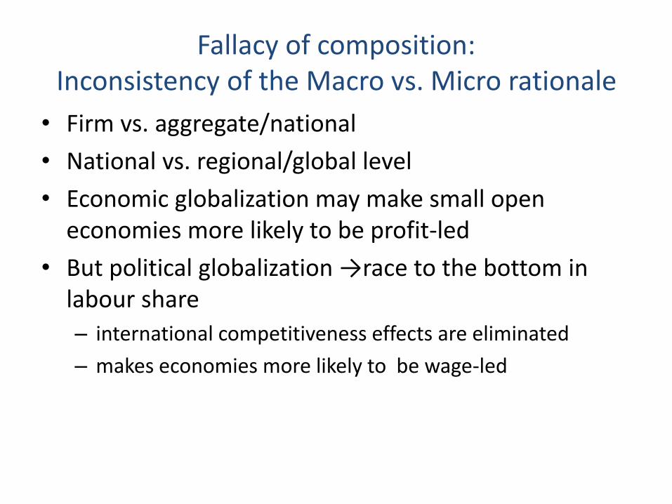
Fallacy of composition: Inconsistency of the Macro vs. Micro rationale

• Firm vs. aggregate/national

• National vs. regional/global level

• Economic globalization may make small open economies more likely to be profit-led

• But political globalization →race to the bottom in labour share

– international competitiveness effects are eliminated

– makes economies more likely to be wage-led

National and Global Multiplier effects

The coefficient estimates in Tables 1, 2, and 6

give the elasticities of C, I, and M with respect to Y ( CYe , IYe , MYe ).

For the elasticity of C with respect to Y, CYe ,:

CYe is calculated as )1( CWCR ee ,

where CRe and CWe are the elasticity of C wrt R and W.

CYe is a weighted average of the elasticities of C wrt R and W,

weights are the shares of R and W in Y (at sample mean).

Again the elasticities have to be converted into partial effects. e.g.:

i

i

i

i

i

i

i

i

i

i

iCYC

Y

Y

C

Y

Y

C

C

Y

Ce

log

log

(D.4)

i

i

iCY

i

i

Y

Ce

Y

C

(D.5)

Finally Hii=i

i

iMY

i

i

iYI

i

i

iCY

i

i

i

i

i

i

Y

Me

Y

Ie

Y

Ce

Y

M

Y

I

Y

C

. (D.6)

If the change in the profit share is isolated to a single country only,

the total effects of a change in πi on equilibrium aggregate demand

=private excess demand (Eii) * the standard multiplier:

ii

ii

i

i

i

i

i

i

i

ii

i

ii

i

i

i

ii

H

E

Y

M

Y

I

Y

C

YNXYIYC

d

YdY

1

1

)/()/()/(

/

(D.7)

1/(1-

i

i

i

i

i

i

Y

M

Y

I

Y

C )

the standard national multiplier

and is expected to be positive for stability.

Global Multiplier

THE MODEL WITH GOVERNMENT

Consumption

Consumption(C) is estimated as a function of adjusted after-

tax profits((1-tr)R), adjusted after-tax wages((1-tw)W) and

social benefits in cash/ other current transfers(B+CTO) which

augment disposable income of HH

If the regime is wage-led a more progressive tax system

(taxes on capital increasing while those on labourdecreasing) increases the impact on demand (Blecker, 2002)

37

Investment

Private investment depends positively on private output and

the after-tax profit share

Total Government expenditure enhances private investment

through demand and crowding in effects (Commendatore,

2011; Seguino, 2012)

Alternative specification: disagregate G in social and

physical infrastructure and other current spending

Private investment depends negatively on public debt to

GDP (crowding out) (Dutt, 2013; Tavani and Zamparelli, 2015)

Domestic and Export Prices, Exports, Imports

𝑙𝑜𝑔𝑃 = 𝑝0 + 𝑝𝑢𝑙𝑐 𝑙𝑜𝑔 𝑢𝑙𝑐 + 𝑝𝑚 𝑙𝑜𝑔 𝑃𝑚 + 𝑝𝑡𝑐 log(1 + 𝑡𝑐)

Greenwich Political Economy Research Centre

Government

𝐺 = 𝜅𝑔𝑌

𝑇 = 𝑡𝑤𝑊 + 𝑡𝑟𝑅 + 𝑡𝑐𝐶

𝐷 = 𝐷−1 + 𝐺𝑡𝑜𝑡 + 𝑟𝐷−1 − 𝑇

Post-Kaleckian Feminist Model: short run and long runOnaran, Oyvat, Fotopoulou 2018

Open economy with 2 sectors: “social sector” & the rest of the economyand male and female workers and capital

• Effect of income distribution (wages vs profits and male vs female wage gaps) on consumption, investment, and net exports

• Effect of public spending in physical vs social infrastructure →Demand side effect in the short run and long run→Long run supply side effect on productivity

– wages, demand, public spending →productivity↑ → moderates the effect of wages on the profit share

• Demand and productivity affect employment of men and women

Gender equality and growth

• Equality is not only a desirable social goal in itself but may also contribute to economic growth and development via

– Demand side effects on growth and investment: Short and long run

– Supply side via effects on productivity: Long run

• Consumption ↑ as equality ↑

– Not just the level but also composition of consumption may change

– more income in the hands of women →household spending on children’s education and health…↑

– Social infrastructure=positive function of gender equality

• Private investment↑ as social infrastructure→productivity↑ & demand↑

– Public + household spending in social infrastructure

• wage share↑ & gender gaps↓→ upward convergence & ↑equality

– →higher growth in a wage-led economy

– Wage-led growth = Equality-led growth

42

Estimation strategy Single • equation approach

Lag structure: contempraneous & • 1 lag, keeping only significant vars with expected sign

A kind of General to Specific but not Testing Down (which would be to drop most •insignificant at a time untill all significant, but very sensitive to path and misses relevant specifications)

Test cointegration•

LR relation: yt=b*xt-1

Error: yt-1-b*xt-1

ECM: Δyt =a0+ a1*Δxt + a2*Δx t-1+ a2*Δy t-1+ c2(yt-1 -b*xt-1 )

ECM: Δyt =a0 a1*Δxt + a2*Δx t-1+ a2*Δy t-1+ c2yt-1 + c3*xt-1

Long run coefficient: b=-c3/c2

To test ECM We use the t• -ratios reported by Banerjee et al. (1998) for the speed of adjustment coefficient (c2) to test the significance of cointegration.

if no cointegration, SR estimation in differences

If SR: long run coefficient= • Σcoeff. of lags/(1- Σ coeff of lagged dependent var)

if WS (and • π ) stationary, then use level (check cointegration only between I&Y)

Wherever there is autocorrelation, either the lagged dependent variable is kept, or •

an AR(1) term is added.

Error correction

term, c2<0

43

Empirical Literature• Systems approach (VAR): Deals with simultaneity, weak in

identifying effects on C and I (few if any control variables)– small effects (Onaran & Stockhammer 05, Korea, Turkey; Stockhammer &

Onaran 04, US, UK, F;) or profit-led demand (Barbosa-Filho & Taylor 06, US; Flaschel & Proano 07)

• Single equation approach: Good in identifying effects, bad in dealing with endogeneity– estimate separate C, I, NX functions

• Bowles & Boyer 95; Naastepad & Storm 07; Hein and Vogel 08: OECD6/8

– estimate separate C, I, X, M, P functions

• Oaran and Galanis 2012, Onaran et al 11, Stockhammer et al 09; Ederer & Sto. 07, Sto. & Ederer 08, Stochammer et al 11: G20, US, Eurozone, France, Austria, Germany respectively

• US: +effects of financialization

• Most find wage-led private domestic demand regimes – Onaran and Galanis 12, Stockhammer et al09, Storm&Naastepad07,

Hein&Vogel08, Stockhammer&Stehrer09

... Estimation strategy The single• -equation approach allows for a flexible modelling of the individual behavioural equations.

three issues, which may cause a bias in the estimations. •

• 1. functional income distribution is assumed to be exogenous. Obviously this is not the case, e.g. lower growth and higher unemployment will have a negative effect on the wage share; however this works usually with a time lag. By assuming exogeneity, we are implying that the time lag of this effect is longer than one year. Endogenizing income distribution is not feasible in the absence of good instrumental variables and long time series data, which could allow for using own lags of the distribution variables as instruments.

• 2. the single equation approach fails to utilize the fact that consumption, investment and net exports add up to private demand.

The main alternative, a VAR approach would require substantially simplifying the •

model as these models cannot handle more than five endogenous variables. Such simplification is likely to lead to misspecification of the behavioural functions. Furthermore the results of VAR estimations are more difficult to interpret. It is not possible to detect and decompose the precise economic relationships that lead to changes in demand in response to distribution. Nevertheless, the convenience of interpretation of the results of the single equation approach comes at the price of some potential bias because the system-dimension and endogeneity are ignored.

... Estimation strategy • 3. the global effects are calculated based on the

separately estimated effects for each country.

Revised version: test Seemingly Unrelated •

Regression (correlated errors) estimated as a system of all equations for C (also for I, X, M, Px, P) for all countries with the selected equations (that survived the General to Specific based on individual country estimations!)

however the correlation of the error terms across the •

country specific equations were not significant; thus we could not reject the hypothesis of independence.

46

Data• annual, 1960/70-2007; AMECO, OECD, WB, ILO, MOSPI, UNIDO, China National

Statistics Office, Molero Simarro 11, Lindenboim et al 11,

• Link adjusted & unadjusted WS for Argentina 1970-92, 2006-07, South Africa 1970-88, 2005-07

• Use mixed income for India and China

•

Consumption

c t-value dlog(Rt) t-value dlog(Wt) t-value DW R2 Sample

Euro area-12 0.006 3.110 0.127 3.716 0.739 15.406 1.871 0.873 1961 2007

Germany 0.007 2.439 0.091 1.576 0.714 10.162 1.954 0.713 1961 2007

France 0.007 3.153 0.137 4.717 0.640 10.770 2.120 0.771 1961 2007

Italy 0.008 2.474 0.167 4.101 0.711 8.621 1.515 0.705 1961 2007

Australia 0.017 4.394 0.098 3.295 0.440 5.463 1.831 0.411 1961 2007

c t-value dlog(Rt) t-value dlog(Wt) t-value ar(1) t-value DW R2 Sample

UK 0.006 1.501 0.162 5.200 0.735 6.852 0.331 2.173 1.838 0.683 1962 2007

Canada 0.007 1.911 0.160 6.268 0.659 6.852 0.411 2.904 1.935 0.725 1962 2007

c t-value dlog(Rt) t-value dlog(Wt) t-value dlog(Rt-1) t-value dlog(Wt-1) t-value dlog(Ct-1) t-value DW R2 Sample

US 0.012 4.048 0.181 4.968 0.536 6.509 -0.114 -2.523 -0.140 -1.389 0.247 1.517 2.017 0.822 1962 2007

c t-value dlog(Rt-1) t-value dlog(Wt-1) t-value DW R2 Sample

Japan 0.011 2.256 0.083 2.103 0.611 6.747 2.300 0.599 1962 2007

c t-value dlog(Rt) t-value dlog(Wt) t-value dlog(Rt-1) t-value dlog(Wt-1) t-value dlog(Ct-1) t-value DW R2 Sample

Turkey 0.008 0.506 0.328 2.840 0.316 2.432 0.088 0.688 0.275 1.824 -0.151 -0.873 1.803 0.320 1972 2006

c t-value dlog(Rt) t-value dlog(Wt) t-value DW R2 Sample

Korea -0.004 -0.411 0.072 3.820 0.845 7.603 2.073 0.641 1971 2007

Argentina 0.003 0.575 0.430 7.927 0.579 13.903 1.944 0.855 1971 2007

c t-value dlog(Rt) t-value dlog(Wt) t-value AR(1) t-value DW R2 Sample

Mexico 0.006 1.263 0.376 7.625 0.566 17.015 0.477 3.021 1.878 0.905 1972 2007

c t-value dlog(Rt) t-value dlog(Wt) t-value dlog(Rt-1) t-value dlog(Wt-1) t-value DW R2 Sample

China -0.014 -0.690 0.443 3.730 0.400 1.629 -0.198 -1.604 0.375 1.702 2.020 0.593 1980 2007

c t-value dlog(Rt) t-value dlog(Wt) t-value dlog(Rt-1) t-value dlog(Wt-1) t-value dlog(Yat) t-value dlog(Yat-1) t-value DW R2 Sample

India 0.003 0.530 0.123 3.270 0.586 4.317 0.028 0.903 0.158 1.319 -0.009 -0.100 -0.168 -2.324 1.894 0.809 1972 2007

c t-value dlog(Rt) t-value dlog(Wt) t-value dlog(Yat) t-value DW R2 Sample

South Africa 0.009 2.939 0.312 9.030 0.785 10.101 -0.061 -3.400 1.926 0.781 1971 2007

The effects of a 1%-point increase in the profit shareWage led

C/Y I/Y X/Y M/Y NX/Y

% change in

total private

excess

demand

Euro zone-12 -0.439 0.299 0.057 0.000 0.057 -0.084

Germany -0.501 0.376 0.096 0.000 0.096 -0.029

France -0.305 0.088 0.036 -0.162 0.198 -0.020

Italy -0.356 0.130 0.037 -0.089 0.126 -0.100

United Kingdom -0.303 0.120 0.048 -0.110 0.158 -0.025

United States -0.426 0.000 0.006 -0.031 0.037 -0.388

Japan -0.353 0.284 0.028 -0.026 0.055 -0.014

Canada -0.326 0.182 0.063 -0.203 0.266 0.122

Australia -0.256 0.174 0.049 -0.223 0.272 0.190

The effects of a 1%-point increase in the profit share

C/Y I/Y X/Y M/Y NX/Y

% change in

total private

excess demand

Turkey -0.491 0.000 0.140 -0.144 0.283 -0.208

Mexico -0.438 0.153 0.128 -0.253 0.381 0.096

Korea -0.422 0.000 0.178 -0.181 0.359 -0.063

Argentina -0.153 0.015 0.014 -0.178 0.192 0.054

China -0.412 0.000 1.095 -0.891 1.986 1.574

India -0.291 0.000 0.080 -0.230 0.310 0.018

South Africa -0.145 0.129 0.000 -0.506 0.506 0.490

Table 10 Elasticities of C, I, and M with respect to Y

h Multiplier

Euro area-12 0.551 1.020 2.035 0.371 1.590

Germany 0.516 0.913 1.911 0.071 1.076

France 0.494 2.050 1.963 0.280 1.388

Italy 0.539 2.610 2.136 0.422 1.730

United Kingdom 0.579 1.311 1.859 0.167 1.200

United States 0.387 3.105 1.996 0.519 2.080

Japan 0.464 1.840 1.136 0.584 2.407

Canada 0.499 1.780 1.505 0.176 1.214

Australia 0.324 2.021 1.886 0.291 1.410

Turkey 0.457 3.343 1.684 0.547 2.208

Mexico 0.471 1.406 2.591 0.097 1.108

Korea 0.725 2.509 2.265 0.452 1.824

Argentina 0.508 0.894 2.868 0.276 1.381

China 0.553 1.664 1.501 0.137 1.159

India 0.639 1.561 1.075 0.541 2.180

South Africa 0.632 1.176 1.199 0.214 1.272

CYeYIe MYe

Y

Me

Y

Ie

Y

Ceh MYYICY

Summary of the multiplier effects at the national and global level

global GDP↓ by 0.36%

The effect of a 1%-point

increase in the profit

share in only one country

on private excess

demand/Y

The effect of a 1%-point increase

in the profit share in only one

country on % change in aggregate

demand (A*multiplier)

The effect of a

simulataneous 1%-point

increase in the profit

share on the % change in

aggregate demand

(including effects of trade

partners' export prices and

GDP))

A B D

Euro area-12 -0.084 -0.133 -0.245

United Kingdom -0.025 -0.030 -0.214

United States -0.388 -0.808 -0.921

Japan -0.014 -0.034 -0.179

Canada 0.122 0.148 -0.269

Australia 0.190 0.268 0.172

Turkey -0.208 -0.459 -0.717

Mexico 0.096 0.106 -0.111

Korea -0.063 -0.115 -0.864

Argentina 0.054 0.075 -0.103

China 1.574 1.932 1.115

India 0.018 0.040 -0.027

South Africa 0.490 0.729 0.390

A wage-led recovery scenario (Onaran and Galanis 2012)

Global GDP↑ by 3.05%

Change in profit

share

The % change in

aggregate demand

(includes national and

global multiplier

effects, i.e. changes in

Pm and Yrw)

Euro area-12 -11.05 2.36

United Kingdom -7.83 1.91

United States -6.31 6.15

Japan -16.71 1.49

Canada -3.00 2.84

Australia -3.00 0.03

Turkey -18.41 10.81

Mexico -3.00 1.45

Korea -8.64 7.46

Argentina -3.00 1.27

China -1.00 5.56

India -3.00 0.43

South Africa -1.00 1.93

Scenario 2

Source: Onaran and Galanis (2012)

Conclusion -1• Domestic demand (consumption+investment) is wage-led (for both the

developed and developing countries).• Large/relatively closed economies are rather wage-led

– ↑wage share : egalitarian; does not harm growth potential • Global simulation: the limits of strategies of international competitiveness

based on wage competition in a highly integrated global economy• Some profit-led economies also contract as an outcome of race to the

bottom (Canada, India, Mexico and Argentina)

• Macro – micro conflict/fallacy of composition : firm vs. aggregate & national vs. European/global

– Globalization=race to the bottom in wage share→likelihood of wage-led regime↑

• Wage/macro policy coordination and avoid beggar thy neighbor policies

• Developing countries: Space for domestic-demand led & more equal growth

– Alternative to pure export-led growth ; south-south cooperation

• Recovery led by domestic demand & ↑ in the wage share

• However: limits to increasing wage share and full employment in capitalism

– Solution of the realization crisis →profit squeeze

– But we are not there yet…

increase public investment by • 1% of GDP

+ wage share by • 1%

+ more progressive taxation (• 1% higher tax on capital and 1% lower tax on labour)

The impact of wage policies is positive but small •

the overall stimulus becomes much stronger with fiscal expansion.•

The effects are stronger if policies are implemented simultaneously in all •

the EU countries.

need for wage and fiscal policy coordination•

• →6.7% higher GDP in the EU15, 4.5% higher GDP in the UK,

Policy mix:

public investment, progressive taxation, Increasing equality

Obst, Onaran, Nikolaidi 2017

Private investment increases by • 2.3% as a ratio to GDP in the EU,

and by 0.9% in the UK

Public spending crowds in private investment, it does not crowd out–

>Demand–

>improved business environment–

Budget balance improves by • 0.9% as a ratio to GDP in the EU, and 0.1% in the UK

Impact on inflation is very modest•

a – 1%-point rise in the wage share →1.5% ↑in prices in the EU, and 2%↑in prices in the UK

•

...Policy mix:

public investment, progressive taxation, Increasing equality

Obst, Onaran, Nikolaidi 2017

Short-term demand vs. long run potential growth and productivity(Onaran, Oyvat, Fotopoulou 2018)

• Long Run: productivity increases when wages, demand and investment increase.

• Productivity needs investment but increasing profits does not always lead to higher private investment

– Investment is more sensitive to demand and lower wages ->low demand

– Investment is not profit-led in many countries (Obst, Onaran, Nikolaidi 2017)

• inequality→lower productivity & potential growth

• Low road labour market policies and low wages also lead to low productivity in LR

• High road labour market policies and high wages → high productivity in LR

• +Public spending →higher employment is feasible with higher wages

Conclusion -2

• Equitable and sustainable development needs green and purple public investment, progressive taxation and pay rise for both women and men!

• Advice:

• Take care of full employment, decent pay for women and men, equality, and ecological sustainability, and the budget will take care of itself.

Long run? Michal Kalecki on

“Political Aspects of Full Employment,” 1943

• “the maintenance of full employment would cause social and political changes which would give a new impetus to the opposition of the business leaders. Indeed, under a regime of permanent full employment, the 'sack' would cease to play its role as a 'disciplinary’ measure. The social position of the boss would be undermined, and the self-assurance and class-consciousness of the working class would grow. ... It is true that profits would be higher under a regime of full employment than they are on the average under laissez-faire... But 'discipline in the factories' and 'political stability' are more appreciated than profits by business leaders. Their class instinct tells them that lasting full employment is unsound from their point of view, and that unemployment is an integral part of the 'normal' capitalist system.”

• Laski citing Kalecki on Poland in the 1950s: “I would rather see people queue for goods than for jobs”.

In the long run?

• Keynes: “in the long run we are all dead”

• Short run unstable: save capitalism from capitalism itself

• Can policy save capitalism from capitalism itself?

• Marx: profit squeeze? Limits to capitalism?

• Kalecki: Full employment not consistent with capitalism

• similar to Marx & Stiglitz?

• Ecological economists (e.g. Victor): Limits to growth?

• Managing with lower growth?

– shorter working hours?

» Keynes, 1930, “Economic Possibilities for our Grandchildren”: “Three-hour shifts or a fifteen-hour week may put off the problem for a great while.”

• Green jobs• Feminist economics: Care crisis and ecological crisis needs purple jobs

➢ Social infrastructure (eg care): More labour intensive; more jobs with lower growth; way to solve also gender inequality crisis

• Synthesis and policy informed by multiple theories?

Planet earth has not traded with Mars but still grew despite declining wage share until the Great Recession.

How?• Potential crisis of aggregate demand deficiency

• The expected outcome should have been a stagnation of global

demand and growth

• This was mainly circumvented by two distinct growth models

• a root cause of the great recession

Debt-led growth Export-led growth

Center US, UK, Australia, New Zealand

Germany, Japan, Netherlands,

Norway, Sweden, Austria, Canada,

Finland, Belgium, Denmark

Periphery

Spain, Greece, Turkey, Portugal,

South Africa, Ireland, Hungary, Czech

Rep., Slovakia, Estonia, Cyprus,

Slovenia

China, Korea

Fragile → Great Recession 2008-2013

Distributional issues are at the very root of the recent crisis

Income Inequality Wealth Concentration

Two growth models(to circumvent stagnant demand)

Debt-ledgrowth

Export-ledgrowth

Trade deficits &capital inflows

Trade surpluses & capital outflows

House price bubble

ABS / CDOs

Demand for investible securities

Household debt

Other factors(deregulation, policy errors, market

failures, boom thinking)

Yields traditional securities

Source: Goda, Onaran, Stockhammer, 2013

Appendix

Notes• we checked the robustness of the results with respect to the adjusted wage

share variable, since adjusting for the labour income of the self-employed is a challenge particularly for the developing countries. When the estimations are done using unadjusted wage share, the MPC differences are in general lower. This indicates that it is intuitively correct to adjust for the labour income of the self employed: MPC from unadjusted profit income is much higher compared to that out of adjusted profit income, since unadjusted profits incorporate self employed labour income with a relatively higher MPC. Nevertheless in most countries this does not lead to a change in the character of the regime. However in Korea, when unadjusted wages are used, the regime seems to be profit-led rather than wage-led primarily due to much lower MPC differences. In Mexico, the effect of the profit share on investment becomes insignificant, and therefore the regime seems to be wage-led rather than profit-led. Overall, these differences do not affect the global results.

Investment

c t-value dlog(Yt) t-value dlog(πt) t-value dlog (It-1) t-value log (It-1) t-value log(Yt-1) t-value log(πt-1) t-value DW R2 Sample

Euro area-12 -0.304 -1.916 2.238 9.801 -0.137 -0.920 0.088 1.105 -0.203 -4.272 0.207 4.545 0.093 2.356 1.820 0.865 1962 2007

Germany -0.136 -0.628 1.805 6.398 0.058 0.284 0.183 1.683 -0.292 -3.756 0.266 4.283 0.172 2.050 1.829 0.748 1962 2007

c t-value dlog(πt-1) t-value dlog(Yt) t-value ar(1) t-value DW R2 Sample

France -0.027 -2.654 0.139 1.657 2.050 10.505 0.670 5.569 1.832 0.822 1963 2007

c t-value log(πt-1) t-value dlog(Yt) t-value dlog(Yt-1) t-value DW R2 Sample

Italy 0.229 5.449 0.241 6.084 2.094 8.819 0.516 2.421 2.524 0.622 1962 2007

c t-value log(πt-1) t-value dlog(Yt) t-value log (It-1) t-value log(Yt-1) t-value DW R2 Sample

UK -1.143 -2.500 0.212 2.513 1.660 5.429 -0.350 -3.392 0.458 3.278 1.870 0.593 1961 2007

c t-value dlog(πt-1) t-value dlog(Yt) t-value dlog(Yt-1) t-value ar(1) t-value DW R2 Sample

US -0.061 -4.519 0.077 0.510 2.738 14.501 0.367 1.824 0.612 4.817 1.697 0.858 1963 2007

c t-value dlog(πt) t-value dlog (It-1) t-value dlog(Yt) t-value dlog(Yt-1) t-value DW R2 Sample

Japan -0.019 -2.845 0.185 2.615 0.485 3.806 1.982 12.339 -1.034 -3.221 2.126 0.924 1962 2007

c t-value dlog(πt-1) t-value dlog(Yt) t-value DW R2 Sample

Canada -0.020 -1.711 0.318 1.874 1.780 6.018 1.593 0.530 1962 2007

c t-value dlog(πt) t-value dlog(Yt) t-value DW R2 Sample

Australia -0.025 -1.550 0.256 1.857 2.021 5.031 1.821 0.494 1961 2007

c t-value log(πt) t-value dlog(Yt) t-value DW R2 Sample

Turkey -0.056 -0.547 0.041 0.294 3.343 6.456 1.743 0.567 1971 2006

c t-value log(πt) t-value log(πt-1) t-value dlog(Yt) t-value dlog(Yt-1) t-value log (It-1) t-value log(Yt-1) t-value DW R2 Sample

Argentina 0.135 0.111 0.190 2.596 -0.147 -2.165 2.808 19.169 0.325 2.001 -0.164 -3.138 0.147 1.895 1.982 0.943 1972 2007

c t-value dlog(Yt) t-value dlog(πt) t-value dlog(πt-1) t-value dlog (It-1) t-value log (It-1) t-value log(Yt-1) t-value log(πt-1) t-value DW R2 Sample

Mexico -1.778 -2.722 3.336 13.407 -0.349 -2.044 -0.259 -1.511 -0.040 -0.616 -0.343 -4.383 0.482 3.765 0.170 1.973 2.506 0.923 1972 2007

c t-value dlog(πt-1) t-value dlog(Yt) t-value dlog (Igt) t-value DW R2 Sample

Korea -0.110 -5.834 -0.011 -0.311 2.509 10.320 0.186 1.960 1.589 0.816 1972 2007

c t-value dlog(πt) t-value dlog(Yt) t-value DW R2 Sample

China -0.006 -0.064 0.030 0.027 1.664 1.703 1.823 0.126 1982 2007

c t-value dlog(πt) t-value dlog(Yt) t-value dlog (Igt-1) t-value DW R2 Sample

India -0.018 -0.682 -0.164 -1.190 1.561 3.856 0.402 2.868 2.369 0.421 1972 2007

c t-value dlog(πt-1) t-value dlog(Yt) t-value dlog (It-1) t-value log (It-1) t-value log(Yt-1) t-value log(πt-1) t-value DW R2 Sample

South Africa -2.249 -1.290 -0.283 -1.917 2.512 6.178 0.317 2.795 -0.343 -4.659 0.403 3.796 0.238 1.709 2.243 0.798 1972 2007

Domestic Prices

c t-value dlog(ULCt-1) t-value dlog(Pmt) t-value DW R2 Sample

Euro area-12 0.014 3.518 0.624 7.846 0.123 2.915 1.515 0.747 1962 2007

Italy 0.018 3.525 0.604 9.320 0.202 4.988 1.731 0.827 1962 2007

UK 0.018 3.018 0.568 6.713 0.190 2.993 2.039 0.691 1962 2007

Japan 0.013 3.227 0.516 6.833 0.095 3.100 1.666 0.630 1962 2007

Canada 0.016 3.983 0.459 5.335 0.257 4.481 1.447 0.678 1962 2007

c t-value dlog(ULCt) t-value dlog(Pmt) t-value DW R2 Sample

Germany 0.012 8.103 0.618 16.023 0.031 1.428 1.491 0.864 1961 2007

c t-value dlog(ULCt-1) t-value dlog(Pt-1) t-value dlog(Pmt) t-value DW R2 Sample

France 0.007 2.360 0.275 2.141 0.522 3.394 0.086 3.281 1.809 0.907 1962 2007

c t-value dlog(ULCt-1) t-value dlog(Pt-1) t-value dlog(Pmt) t-value dlog(Pmt-1) t-value DW R2 Sample

US 0.009 5.219 0.211 2.710 0.429 4.836 0.109 8.403 0.044 2.590 1.745 0.951 1962 2007

c t-value dlog(ULCt) t-value dlog(Pmt) t-value dlog(Pmt-1) t-value DW R2 Sample

Australia 0.016 4.324 0.624 8.856 -0.031 -0.579 0.150 3.429 1.976 0.814 1962 2007

c t-value dlog(ULCt) t-value dlog(Pt-1) t-value dlog(Pmt) t-value DW R2 Sample

Turkey 0.011 0.643 0.354 5.402 0.263 4.280 0.364 7.124 2.196 0.949 1972 2006

c t-value dlog(ULCt) t-value dlog(ULCt-1) t-value dlog(Pt-1) t-value dlog(Pmt) t-value DW R2 Sample

Mexico 0.008 0.884 0.700 8.642 -0.265 -2.136 0.309 2.875 0.261 7.178 2.387 0.979 1972 2007

c t-value dlog(ULCt) dlog(Pmt) t-value dlog(Pmt-1) t-value DW R2 Sample

Korea 0.016 3.026 0.735 10.508 0.073 1.709 0.095 2.685 1.887 0.912 1972 2007

c t-value dlog(ULCt) t-value dlog(Pmt) t-value DW R2 Sample

Argentina 0.002 0.162 0.640 17.025 0.359 9.597 1.828 0.994 1971 2007

China 0.010 2.126 0.832 12.990 0.022 0.660 1.289 0.883 1979 2007

India 0.023 5.114 0.756 12.205 0.009 0.401 2.020 0.854 1971 2007

South Africa 0.033 2.611 0.618 5.634 0.124 1.946 1.897 0.567 1971 2007

c t-value dlog(ULCt-1) t-value dlog(Pxt-1) t-value dlog(Pmt) t-value DW R2 Sample

Euro area-12 0.003 1.670 0.165 3.141 0.102 2.504 0.566 27.168 1.586 0.970 1962 2007

Germany 0.004 1.557 0.216 2.845 0.214 2.631 0.355 9.780 1.719 0.813 1962 2007

Italy 0.004 0.960 0.178 2.616 0.156 2.695 0.569 19.040 2.495 0.946 1962 2007

c t-value log(Pxt-1) t-value log(ULCt-1) t-value log(Pmt-1) t-value dlog(ULCt) t-value dlog(Pmt) t-value ar(1) t-value dw r2 Sample

France 0.429 3.756 -0.663 -4.558 0.098 1.710 0.475 5.253 -0.117 -1.131 0.545 17.814 0.722 4.160 1.760 0.962 1962 2007

c t-value log(Pxt-1) t-value log(ULCt-1) t-value log(Pmt-1) t-value dlog(ULCt) t-value dlog(Pmt) t-value dw r2 Sample

United Kingdom 0.043 1.592 -0.412 -3.895 0.061 2.120 0.342 4.132 0.179 2.378 0.575 12.748 1.600 0.924 1961 2007

United States 0.374 3.479 -0.352 -3.238 0.049 1.973 0.223 3.214 0.397 2.765 0.489 11.547 1.929 0.913 1961 2007

c t-value dlog(ULCt) t-value dlog(Pmt) t-value DW R2 Sample

Japan -0.012 -4.226 0.313 5.610 0.389 16.889 2.023 0.921 1961 2007

Australia 0.014 1.263 0.374 1.798 0.316 2.121 1.625 0.352 1961 2007

c t-value dlog(ULCt) t-value dlog(ULCt-1) t-value dlog(Pmt) t-value DW R2 Sample

Canada 0.004 0.632 0.620 3.209 -0.472 -2.712 0.820 8.822 1.932 0.795 1962 2007

Export Prices

c t-value dlog(ULCt-1) t-value dlog(Pmt) t-value DW R2 Sample

Turkey -0.013 -0.395 0.179 1.827 0.868 9.972 2.277 0.851 1972 2007

c t-value dlog(ULCt) t-value dlog(Pmt) t-value DW R2 Sample

Mexico 0.014 0.830 0.260 2.514 0.675 9.619 2.112 0.925 1971 2007

Argentina 0.014 0.913 0.107 2.858 0.878 23.456 2.014 0.994 1971 2007

China -0.008 -0.745 0.315 2.166 1.035 13.921 1.771 0.904 1979 2007

India 0.022 1.259 0.693 2.879 0.109 1.322 1.711 0.342 1971 2007

c t-value dlog(ULCt) t-value dlog(Pxt-1) t-value dlog(Pmt) t-value DW R2 Sample

Korea -0.013 -1.578 0.336 2.911 0.009 0.127 0.614 9.198 1.703 0.886 1972 2007

c t-value dlog(ULCt) t-value dlog(Pmt) t-value ar(1) t-value DW R2 Sample

South Africa 0.068 1.660 -0.529 -1.516 0.957 6.374 0.357 1.995 1.699 0.616 1972 2007

c t-value dlog(Px/Pmt) t-value dlog(Xt-1) t-value dlog(Yrwt) t-value dlog(Et) t-value DW R2 Sample

Euro area-12 -0.021 -1.042 -1.304 -4.813 0.161 1.460 1.884 3.821 0.141 1.916 1.683 0.643 1971 2007

France -0.030 -2.151 -0.314 -2.204 0.265 2.466 2.065 5.952 0.172 2.016 1.765 0.601 1971 2007

c t-value dlog((Px/Pm)t-1) t-value dlog(Yrwt) t-value DW R2 Sample

Germany 0.000 0.002 -0.428 -1.967 1.779 2.911 2.121 0.207 1971 2007

c t-value dlog(Px/Pmt) t-value dlog(Yrwt) t-value DW R2 Sample

Italy -0.005 -0.266 -0.273 -1.760 1.554 3.028 1.863 0.308 1971 2007

UK 0.011 0.821 -0.519 -3.771 1.057 2.885 1.636 0.443 1971 2007

Japan 0.014 0.617 -0.428 -4.039 1.293 1.984 2.169 0.355 1971 2007

Australia 0.036 1.782 -0.235 -1.891 0.472 0.779 1.944 0.095 1971 2007

c t-value dlog(Px/Pmt) t-value dlog(Yrwt) t-value dlog(Et-1) t-value ar(1) t-value DW R2 Sample

US -0.037 -1.990 -0.286 -2.182 2.935 6.099 0.113 2.051 0.517 3.427 2.315 0.727 1972 2007

c t-value dlog((Px/Pm)t-1) t-value dlog(Xt-1) t-value dlog(Yrwt) t-value DW R2 Sample

Canada -0.026 -1.498 -0.558 -2.774 0.172 1.371 2.056 4.163 1.648 0.495 1971 2007

Exports

c t-value dlog(RULCt-1) t-value dlog(Yrwt) t-value DW R2 Sample

Turkey 0.051 0.794 -0.557 -1.903 0.899 0.488 2.454 0.100 1972 2007

c t-value dlog(RULCt) t-value dlog(Yrwt) t-value ar(1) t-value DW R2 Sample

Mexico 0.005 0.160 -0.436 -2.095 2.395 3.067 0.463 2.713 1.912 0.382 1972 2007

c t-value log(Xt-1) t-value log(Px/Pmt-1) t-value log(Yrwt-1) t-value dlog(Px/Pmt) t-value dlog(Xt-1) t-value dlog(Yrwt) t-value DW R2 Sample

Korea -42.041 -3.741 -0.396 -4.009 -0.198 -1.713 1.510 3.769 0.256 0.964 0.082 0.592 3.213 3.262 1.616 0.586 1972 2007

c t-value dlog(Px/Pmt) t-value dlog(Xt-1) t-value dlog(Yrwt) t-value DW R2 Sample

Argentina -0.053 -1.397 -0.318 -1.712 0.091 0.611 3.433 3.148 1.715 0.257 1972 2007

China 0.010 0.195 -1.175 -3.200 0.396 2.556 2.584 1.742 1.900 0.457 1980 2007

India 0.084 2.371 -0.253 -2.364 0.185 1.165 -0.220 -0.229 1.899 0.177 1972 2007

c t-value dlog(Px/Pmt) t-value dlog(Yrwt) t-value DW R2 Sample

South Africa -0.007 -0.373 -0.126 -1.036 1.101 1.876 1.457 0.096 1971 2007

Imports

c t-value dlog((P/Pm)t-1) t-value dlog(Yt) t-value DW R2 Sample

Euro area-12 -0.008 -0.433 0.236 1.182 2.035 3.450 1.537 0.329 1962 2007

Italy -0.008 -0.759 0.233 2.390 2.136 6.818 2.219 0.607 1962 2007

Japan 0.010 0.740 0.255 3.299 1.136 4.576 1.835 0.499 1962 2007

c t-value dlog((P/Pm)t-1) t-value dlog(Yt) t-value ar(1) t-value DW R2 Sample

Germany 0.009 0.990 0.005 0.046 1.911 7.083 0.283 1.848 1.903 0.618 1963 2007

c t-value log(Mt-1) t-value log((P/Pm)t-1) t-value log(Yt-1) t-value dlog((P/Pm)t) t-value dlog(Yt) t-value DW R2 Sample

France -2.452 -4.565 -0.292 -3.932 0.140 2.796 0.573 4.330 0.069 0.989 2.923 8.361 2.166 0.782 1961 2007

United Kingdom -2.954 -4.748 -0.414 -4.773 0.130 3.178 0.769 4.814 -0.024 -0.388 1.698 8.584 2.142 0.739 1961 2007

United States -4.610 -4.639 -0.414 -4.422 0.177 3.755 0.826 4.554 0.132 1.651 2.341 9.783 1.905 0.787 1961 2007

c t-value dlog(P/Pmt) t-value dlog(Yt) t-value DW R2 Sample

Australia -0.017 -0.823 0.558 2.964 1.886 3.576 2.081 0.374 1961 2007

c t-value dlog(P/Pmt) t-value dlog(Yt) t-value dlog(Yt-1) t-value dlog(Mt-1) t-value DW R2 Sample

Canada 0.000 -0.008 0.356 2.570 2.503 8.780 -1.636 -4.164 0.424 3.369 2.218 0.675 1962 2007

c t-value dlog(RULCt-1) t-value dlog(Yrwt) t-value DW R2 Sample

Turkey 0.051 0.794 -0.557 -1.903 0.899 0.488 2.454 0.100 1972 2007

c t-value dlog(RULCt) t-value dlog(Yrwt) t-value ar(1) t-value DW R2 Sample

Mexico 0.005 0.160 -0.436 -2.095 2.395 3.067 0.463 2.713 1.912 0.382 1972 2007

c t-value log(Xt-1) t-value log(Px/Pmt-1) t-value log(Yrwt-1) t-value dlog(Px/Pmt) t-value dlog(Xt-1) t-value dlog(Yrwt) t-value DW R2 Sample

Korea -42.041 -3.741 -0.396 -4.009 -0.198 -1.713 1.510 3.769 0.256 0.964 0.082 0.592 3.213 3.262 1.616 0.586 1972 2007

c t-value dlog(Px/Pmt) t-value dlog(Xt-1) t-value dlog(Yrwt) t-value DW R2 Sample

Argentina -0.053 -1.397 -0.318 -1.712 0.091 0.611 3.433 3.148 1.715 0.257 1972 2007

China 0.010 0.195 -1.175 -3.200 0.396 2.556 2.584 1.742 1.900 0.457 1980 2007

India 0.084 2.371 -0.253 -2.364 0.185 1.165 -0.220 -0.229 1.899 0.177 1972 2007

c t-value dlog(Px/Pmt) t-value dlog(Yrwt) t-value DW R2 Sample

South Africa -0.007 -0.373 -0.126 -1.036 1.101 1.876 1.457 0.096 1971 2007

Sum

eP.ULC eULC.RULC ePx.ULC eX.Px eX.RULC RULC Yf/Y X/Y eM.P eM.RULC M/Y

A B C D E (B*C*D) F G H I (-E*G*H/F) J K (A*B*J) L M (K*G*L/F) I-M

Euro area (12 countries)0.624 2.660 0.184 -1.304 -0.637 0.619 0.893 0.062 0.057 0.000 0.000 0.068 0.000 0.057

Germany 0.618 2.617 0.274 -0.428 -0.307 0.615 0.900 0.214 0.096 0.000 0.000 0.209 0.000 0.096

France 0.577 2.363 0.148 -0.428 -0.150 0.615 0.867 0.171 0.036 0.481 0.656 0.175 -0.162 0.198

Italy 0.604 2.527 0.211 -0.273 -0.146 0.623 0.909 0.174 0.037 0.233 0.356 0.172 -0.089 0.126

UK 0.568 2.316 0.148 -0.519 -0.178 0.643 0.885 0.195 0.048 0.313 0.412 0.195 -0.110 0.158

US 0.369 1.585 0.138 -0.286 -0.063 0.634 0.926 0.068 0.006 0.428 0.250 0.085 -0.031 0.037

Japan 0.516 2.066 0.313 -0.428 -0.276 0.673 0.933 0.074 0.028 0.255 0.271 0.070 -0.026 0.055

Canada 0.459 1.849 0.148 -0.558 -0.153 0.601 0.884 0.278 0.063 0.617 0.524 0.264 -0.203 0.266

Australia 0.624 2.661 0.374 -0.235 -0.234 0.597 0.904 0.140 0.049 0.558 0.926 0.159 -0.223 0.272

ImportsExports

YX /

YM /

YNX /

Sum

eP.ULC eULC.RULC ePx.ULC eX.Px eX.RULC RULC Yf/Y X/Y eM.P eM.RULC M/Y

A B C D E (B*C*D) F G H I (-E*G*H/F) J K (A*B*J) L M (K*G*L/F) I-M

Turkey 0.481 1.927 0.179 -1.613 -0.557 0.459 0.937 0.123 0.140 0.546 0.506 0.139 -0.144 0.283

Mexico 0.629 2.695 0.260 -0.621 -0.436 0.466 0.928 0.148 0.128 0.472 0.800 0.159 -0.253 0.381

Korea 0.735 3.779 0.336 -0.500 -0.636 0.753 0.891 0.237 0.178 0.216 0.600 0.255 -0.181 0.359

Argentina 0.640 2.780 0.107 -0.318 -0.095 0.507 0.975 0.079 0.014 0.745 1.327 0.070 -0.178 0.192

China 0.832 5.966 0.315 -1.945 -3.658 0.503 0.867 0.232 1.463 0.795 3.946 0.193 -1.311 2.774

India 0.756 4.106 0.693 -0.253 -0.718 0.753 0.914 0.091 0.080 0.546 1.695 0.112 -0.230 0.310

South Africa 0.618 2.620 0.000 0.000 0.000 0.624 0.921 0.237 0.000 1.002 1.624 0.211 -0.506 0.506

ImportsExports

YX /

YNX /

YM /

Two wage-led recovery scenarios

1. global GDP↑ by 2.81% 2. global GDP↑ by 3.05%

Change in profit

share to preserve

the peak wage

share

The % change in

aggregate demand

(includes national and

global multiplier

effects, i.e. changes in

Pm and Yrw)

Change in profit

share

The % change in

aggregate demand

(includes national and

global multiplier

effects, i.e. changes in

Pm and Yrw)

Euro area-12 -11.05 2.49 -11.05 2.36

United Kingdom -7.83 2.01 -7.83 1.91

United States -6.31 6.47 -6.31 6.15

Japan -16.71 1.77 -16.71 1.49

Canada -7.73 2.44 -3.00 2.84

Australia -9.02 -1.35 -3.00 0.03

Turkey -18.41 11.22 -18.41 10.81

Mexico -22.03 -0.56 -3.00 1.45

Korea -8.64 7.60 -8.64 7.46

Argentina -9.12 0.86 -3.00 1.27

China -8.00 -7.44 -1.00 5.56

India -15.96 0.05 -3.00 0.43

South Africa -13.07 -6.29 -1.00 1.93

Scenario 1 Scenario 2