Post Harvest Handling Methods for Enhanced Competitiveness of Fresh Cut Peonies

Part 1.

Vase Life Studies

Patricia S. Holloway, PhD 2014 Student interns: Ruth Osborne and Makenzie Stamey 2013 Student interns: Melissa Pietila and Kathryn Mihalczo

Part 2. Effect of Boron and Calcium Sprays on Stem Strength of Peonies

Mingchu Zhang. PhD

Robert Van Veldhuizen, Research Associate

University of Alaska Fairbanks School of Natural Resources and Extension

Department of Agriculture and Horticulture Agricultural and Forestry Experiment Station

RESEARCH REPORT

to:

Alaska Department of Natural Resources Division of Agriculture

Alaska Specialty Crops Research Initiative

  2  

Post Harvest Handling Methods for Enhanced Competitiveness of Fresh Cut Peonies

University of Alaska Fairbanks

Patricia S. Holloway Mingchu Zhang

Joint Summary. The University of Alaska Fairbanks in cooperation with Alaska peony

growers conducted a series of experiments to establish standards for best quality fresh cut flowers to meet or exceed rigorous international industry requirements. Preliminary research at UAF found that chilling at 34oF for 1 week, doubled the vase life of peonies, and data from 2013 season corroborates those findings. However, vase life for cut flowers in 2014 decreased significantly and did not improve with chilling. Vase life for ‘Sarah Bernhardt’ and ‘Duchess de Nemours’ peonies averaged 6.1 days and 5.9 days, respectively for the entire treatment period and did not differ from the un-chilled control. Because of the unexpected results from 2014, this research did not clearly identify minimum chilling requirements for Alaska peonies. In contrast, cut stems in 2013 showed a linear increase in vase life with chilling (8.2 to 14.2 days for ‘Sarah Bernhardt’ and 6.9 to 13 days for ‘Duchess de Nemours’. Vase life and bud diameter did not differ among early- mid- and late-season cutting dates for both cultivars. Cut stems from two commercial farms showed the same short vase life, and there was no statistical difference in vase life among farms. These studies do not corroborate the statement that vase life of Alaska peonies is double the national standard. Environmental factors during spring growth or post harvest handling differences play a more significant role in defining vase life than simply hours of chilling (deliverables b,c,e).

Vase  life  for  68  cultivars  in  2014  ranged  from  4  days  to  9  days  (mean  6.0  +  1.0  days).    

In  2013,  vase  life  averaged  nearly  three  days  longer,  8.6  +  2.7  days  (range  4  –  14  days)..  Vase  life  for  2014  was  significantly  lower  for  most  cultivars  than  2013.  In  2013,  more  than  70  percent  of  the  cultivars  showed  an  average  vase  life  of  7  days  or  more,  while  in  2014,  only  24  percent  reached  that  standard.  The  four  main  classifications  of  peonies  grown  at  the  botanical  garden  (semi-­‐double,  Japanese,  bomb  and  full  double)  had  an    average  vase  life  ranging  from  5  days  to  17  days.  One  classification  had  a  vase  life  of  less  than  7  days  for  both  2013  and  2014,  the  Intersectional  hybrids.  (deliverable  1d)  

 Plants  sprayed  with  Boron  (B),  calcium  (Ca)  and  potassium  (K)  showed  foliar  

absorption  of  B,  but  not  Ca  and  K.  No  spray  solution  improved  stem  strength  or  increased  stem  diameter  in  2014.  The  machine  invented  to  determine  bending  distance  prior  to  breaking  fell  short  of  our  goal.  Additional  work  on  methods  of  securing  the  peony  stems  in  the  machine  is  needed  to  reduce  errors.  (deliverable  1a)  

 Part 1. Vase Life Studies

Patricia S. Holloway 2014 Student interns: Ruth Osborne and Makenzie Stamey 2013 Student interns: Melissa Pietila and Kathryn Mihalczo

Introduction  

World cut flower sales are a highly competitive, volatile and multi-billion dollar industry (Highbeam Business 2012, Sarkar 2012, USDA 2013). Sales are subject to

  3  

fashion whims of consumers as well as industry demands for quality blooms that meet bud size standards and ship well; a product that has the requisite stem length/strength; and one with a long vase life. Since the product is a senescing (dying) stem, the industry has the daunting task of delivering a product whose consumer life is as long and colorful as possible (The reported consumer life for peonies is 7 days [Dole and Wilkin 2005]). Cut flowers must meet rigorous standards or they will be replaced by a myriad of other available specialty cuts from around the world (H.R.Kennicott, Kennicott Kutts, Ltd. Chicago, IL. pers. comm. 2012). The Alaska peony industry must meet these standards yet fit with the cultural conditions, climate and distribution system of Alaska. Every stage of plant production, from cultivation, harvest, post harvest handling, and shipping, impacts product quality.

UAF researchers began studying production chain management in 2001 (Auer

2008, Auer & Greenberg 2009, Auer & Holloway 2008, Holloway & Hanscom 2007, Holloway et al. 2003, 2004, 2005, 2010, Holloway & Buchholz 2013, Klingman 2002). The Alaska peony industry reached a milestone in 2012. More than 25,000 fresh cut peonies entered domestic and international markets (Holloway & Buchholz 2013), and production increased to 32,000 stems in 2013 (American Flower Farmer LLC 2014). Alaska growers must know and understand product quality, and a policy of exporting only top grade peonies must be established. Growers need to define what a quality brand is and work toward world recognition.

Preliminary research at UAF found that chilling at 34oF for 1 week doubled the

vase life of peonies, but 12 hours was not sufficient. We want to determine the minimum time necessary for chilling prior to shipping for maximum consumer vase life. Some growers actually ship the day of harvest, which may not lead to the best product. One of our experiments hinted that vase life of Alaska peonies is double that of the Lower 48. We will repeat this experiment to verify those data so growers can demonstrate one more unique feature for marketing Alaska peonies. The UAF Experiment Station has a collection of 110 peony cultivars (Holloway 2013). We will determine the maximum vase life for all these cultivars so growers can rank them for quality. We will also conduct an experiment to identify differences in vase life with ‘Sarah Bernhardt’ peonies from Alaska farms to identify quality variations within the industry. Methods Experiment 1. Impact of cold storage time on vase life of ‘Sarah Bernhardt and Duchess de Nemours’ peonies. Goal: to establish the minimum time necessary for chilling prior to shipping for maximum consumer vase of fresh cut peonies. An experiment (4 replicates, 5 stems per rep) was performed that exposed fresh cut stems of two cultivars, ‘Sarah Bernhardt’, ‘Duchess de Nemours’, to a series of cold treatments (24, 48, 72, 96, 120, 144, 168 hrs in 2013 and 0, 48, 96, 144, 192, 240, 288 and 336 hours in 2014) at a target 34oF degrees.

All stems were harvested from the peony fields at the UAF Georgeson Botanical Garden, Fairbanks, Alaska. Cut stems were harvested beginning 1 July in both 2013 and

  4  

2014, cut to uniform stem length (24 inches), and wrapped in newspaper. In 2013, bundles were moved immediately after processing to a laboratory cooler. In 2014, the refrigeration unit was changed to a Conex cooler with an air conditioner/CoolBot® refrigeration unit/controller. Both environments were equipped with Hobo® data loggers (Onset Computer Corp.) for hourly records of air temperature and relative humidity. In addition, field air and soil temperature and relative humidity were recorded at the Fairbanks Experiment Farm using the same data loggers with sensors at a 30-inch height for air and 6-inch depth for soil.

In 2013, flowers were held in newspaper sleeves, in the dark and un-hydrated for 8 chilling treatments that included a control (no chilling) followed by chilling up to 7 days (24, 48, 72, 96, 120, 144, 168 hours). In 2014, the experiment was extended to 14 days at 2-day intervals (0,48, 96, 144, 192, 240, 288 and 336 hours). Following treatment, the chilled stems were removed from refrigeration and placed in jars of tap water in a laboratory with 24-hr fluorescent lights (25 µM.m2.s-1 measured 4 ft beneath the fixtures) supplemented with natural lighting from laboratory windows, and ambient room temperature. Flowers were observed daily, and, stems were gently tapped to release petals if an abscission layer had formed. The date of petal wilt or petal fall on chilled and un-chilled cut stems was recorded. Air temperature and relative humidity were recorded hourly in cold storage and in the laboratory. Data were analyzed using regression analysis for total vase life and hours of chilling during two cutting seasons, 2013 and 2014. Experiment 2. Vase life of early, mid and late season buds of ‘Sarah Bernhardt’ and ‘Duchess de Nemours’ cultivars. Goal: to establish that Alaska peonies have a vase life that is equal to or significantly longer than the 7 days reported for peonies in world markets and to determine if there are any differences among cutting dates. Peonies of two cultivars, ‘Sarah Bernhardt’ and ‘Duchess de Nemours’, were harvested on three dates, 1, 10 and 20 July, 2014 (6 stems per cultivar, 3 replicates on each date). Half were placed immediately into jars of tap water and the remainder were refrigerated for 7 days in a Conex/CoolBot® cooler. Handling in the cooler and subsequent vase life studies were the same as Experiment 1. Data were analyzed using analysis of variance for chilled and un-chilled flowers for three harvest dates. Experiment 3. Cultivar vase life at the Georgeson Botanical Garden. Vase studies were conducted in 2013 and 2014 on 110 peony cultivars growing at UAF Georgeson Botanical Garden. Goal: show variability among cultivars, identify cultivars with the longest vase life, and show vase life differences among peony classes (single, double, Japanese, semi-double, bomb, Intersectional) by determining optimum vase life compared to national average (7 days). Six cut stems of each cultivar were harvested as they reached Stage 3 bud maturity index (Holloway and Pietila 2012). They were chilled for 7 days, then evaluated for vase life as described in Experiment 1. Cultivars were categorized according to flower classification to learn the range, mean and median vase life for each category. Only cultivars harvested both in 2013 and 2014 were subject to analysis of variance (6 stems per replicate, 3 replicates) for differences among cultivars and years.

  5  

Experiment 4. Vase life trials among commercial Alaska growers. Goal: to identify possible variations in product vase life due to diverse growing, handling and shipping conditions of individual growers. Ten growers in Alaska’s interior were asked to submit 12 randomly cut stems of ‘Sarah Bernhardt’ peonies to a local pack house. These pack houses recorded methods of handling (cooler temperatures, relative humidity) for 7 days after which they were transferred to UAF, placed in jars of tap water, and evaluated for vase life. Results  and  Discussion  

After  the  2014  season,  growers  were  convinced  that  the  2013  and  2014  seasons  were  complete  opposites  in  relation  to  temperatures  and  rainfall,  but  seasonal  average  air  temperatures  were  very  similar  (Table  1).  The  2013  season  was  warmer  in  June  and  July  than  2014,  and  thaw  degree-­‐days  differed  by  only  138  units.  The  most  significant  difference  was  rainfall  that  was  8.61  inches  greater  in  2014  than  2013.  In  2013,  Interior  residents  had  few  complaints  about  the  weather;  it  was  hot  and  dry  early  in  the  season,  then  moderated  in  August  and  September.  All  horticultural  and  agronomic  crops  that  were  not  irrigated  suffered  severe  losses  due  to  water  deficits  in  2013.  In  2014,  temperatures  were  much  cooler  during  the  peak  peony  harvest  season,  and  beginning  about  the  third  week  of  June,  rainfall  was  nearly  constant.  Rainfall  in  2014  eclipsed  the  highest  seasonal  rainfall  recorded  in  the  past  25  years  by  2.71  inches.      Table  1  Temperature  and  rainfall  records  for  the  UAF  Fairbanks  Experiment  Farm  during  2013  and  2014  growing  seasons.      Growing  season  weather  statistics*  

Year  2013   2014  

Average  seasonal  air  temp  (F)*  

53.9   55.9  

Air    temp  (F)  (max  –  min)   92.0  (27  Jun)  –  16.9  (6  May)  

84.2  (  7  Jul)  -­‐  29.3  (30  Aug)  

     May  (mean)  (F)   42.2   48.9        June     64.5   56.4        July   62.8   58.3        Aug   58.2   57.5        Sept   41.9   42.6  Date  of  last  spring  frost   22  May   21  May  Date  of  first  autumn  frost   25  Aug   30  Aug  Previous  Winter  Min  (F)   -­‐45.3  (27  Jan  2013)   -­‐41.6  (13  Jan  2014)  Rainfall  (inches)**   5.42   14.03  Thaw  degree-­‐days  (base  temperature  32F  

3360   3222  

*1  May  –  30  Sept,  from  Agricultural  and  Forestry  Experiment  Station  weather  station.          

  6  

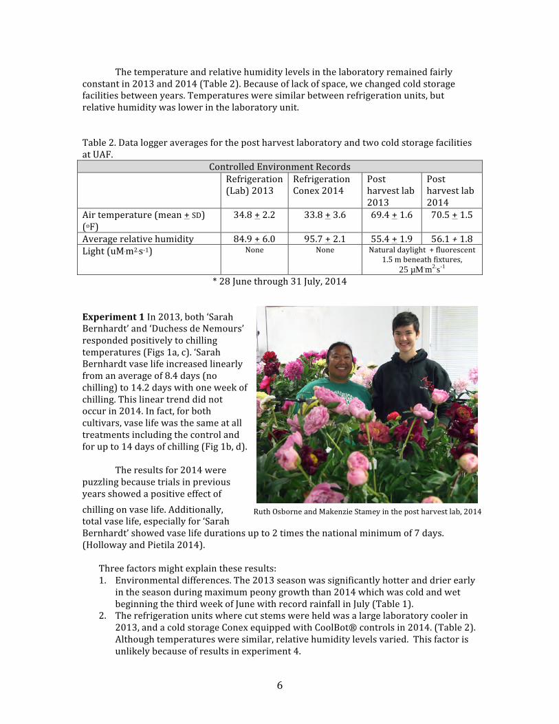
The  temperature  and  relative  humidity  levels  in  the  laboratory  remained  fairly  constant  in  2013  and  2014  (Table  2).  Because  of  lack  of  space,  we  changed  cold  storage  facilities  between  years.  Temperatures  were  similar  between  refrigeration  units,  but  relative  humidity  was  lower  in  the  laboratory  unit.        Table  2.  Data  logger  averages  for  the  post  harvest  laboratory  and  two  cold  storage  facilities  at  UAF.  

Controlled  Environment  Records     Refrigeration    

(Lab)  2013  Refrigeration      Conex  2014  

Post  harvest  lab    2013  

Post  harvest  lab  2014  

Air  temperature  (mean  +  SD)  (oF)  

34.8  +  2.2   33.8  +  3.6   69.4  +  1.6   70.5  +  1.5  

Average  relative  humidity   84.9  +  6.0   95.7  +  2.1   55.4  +  1.9   56.1  +  1.8  Light  (uM.m2.s-­‐1)   None   None   Natural  daylight    +  fluorescent    

1.5  m  beneath  fixtures,    25 µM.m2.s-1

 *  28  June  through  31  July,  2014  

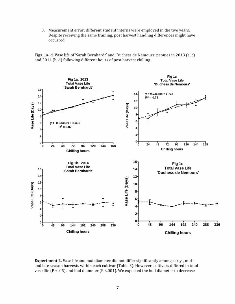
   Experiment  1  In  2013,  both  ‘Sarah  Bernhardt’  and  ‘Duchess  de  Nemours’  responded  positively  to  chilling  temperatures  (Figs  1a,  c).  ‘Sarah  Bernhardt  vase  life  increased  linearly  from  an  average  of  8.4  days  (no  chilling)  to  14.2  days  with  one  week  of  chilling.  This  linear  trend  did  not  occur  in  2014.  In  fact,  for  both  cultivars,  vase  life  was  the  same  at  all  treatments  including  the  control  and  for  up  to  14  days  of  chilling  (Fig  1b,  d).      

The  results  for  2014  were  puzzling  because  trials  in  previous  years  showed  a  positive  effect  of  chilling  on  vase  life.  Additionally,  total  vase  life,  especially  for  ‘Sarah  Bernhardt’  showed  vase  life  durations  up  to  2  times  the  national  minimum  of  7  days.    (Holloway  and  Pietila  2014).    

Three  factors  might  explain  these  results:  1. Environmental  differences.  The  2013  season  was  significantly  hotter  and  drier  early  

in  the  season  during  maximum  peony  growth  than  2014  which  was  cold  and  wet  beginning  the  third  week  of  June  with  record  rainfall  in  July  (Table  1).      

2. The  refrigeration  units  where  cut  stems  were  held  was  a  large  laboratory  cooler  in  2013,  and  a  cold  storage  Conex  equipped  with  CoolBot®  controls  in  2014.  (Table  2).  Although  temperatures  were  similar,  relative  humidity  levels  varied.    This  factor  is  unlikely  because  of  results  in  experiment  4.    

Ruth  Osborne  and  Makenzie  Stamey  in  the  post  harvest  lab,  2014  

  7  

3. Measurement  error:  different  student  interns  were  employed  in  the  two  years.  Despite  receiving  the  same  training,  post  harvest  handling  differences  might  have  occurred.  

   Figs.  1a-­‐  d.  Vase  life  of  ‘Sarah  Bernhardt’  and  ‘Duchess  de  Nemours’  peonies  in  2013  (a,  c)    and  2014  (b,  d)  following  different  hours  of  post  harvest  chilling.      

         Experiment  2.  Vase  life  and  bud  diameter  did  not  differ  significantly  among  early-­‐,  mid-­‐  and  late-­‐season  harvests  within  each  cultivar  (Table  3).  However,  cultivars  differed  in  total  vase  life  (P  <  .05)  and  bud  diameter  (P  <.001).  We  expected  the  bud  diameter  to  decrease  

Fig 1c Total Vase Life

'Duchess de Nemours'

0 24 48 72 96 120 144 1680

2

4

6

8

10

12

14 y = 0.03648x + 6.717 R2 = 0.78

Chilling hours

Vas

e Li

fe (D

ays)

0 48 96 144 192 240 288 3360

2

4

6

8

10

12

14

16 Fig 1d Total Vase Life

'Duchess de Nemours'

Chilling hours

Vas

e Li

fe (D

ays)

Fig 1a. 2013 Total Vase Life

'Sarah Bernhardt'

0 24 48 72 96 120 144 1680

2

4

6

8

10

12

14

16

y = 0.03482x + 8.430 R2 = 0.87

Chilling hours

Vas

e Li

fe (D

ays)

0 48 96 144 192 240 288 3360

2

4

6

8

10

12

14

16

Chilling hours

Vas

e Li

fe (D

ays)

Fig 1b. 2014 Total Vase Life

'Sarah Bernhardt'

  8  

over  the  season,  but  the  selection  was  not  random.  We  chose  the  largest  buds  for  harvest  on  each  date,  and  the  size  did  not  differ.  The  bud  diameter  was  very  consistent  for  each  harvest  date  for  ‘Sarah  Bernhardt’    (very  narrow  standard  deviations).  Bud  diameter  for  ‘Duchess  de  Nemours’  showed  a  much  wider  deviation  from  the  mean  indicating  that  bud  size  varies  widely  on  all  harvest  dates  even  among  the  largest  buds  harvested.          Table  3  Vase  life  of  Sarah  Bernhardt  and  Duchess  de  Nemours  peonies  harvest  at  three  different  dates  during  the  2014  growing  season.      

Vase Life (Days + SD)* Bud diameter (mm + SD)*** Cultivar Early

(1 July) Mid

(8 July) Late

(15 July) Early

(1 July) Mid

(8 July) Late

(15 July) Sarah Bernhardt**

6.4 + 1.2

5.5 + 1.6

6.1 + 1.0

44.6 + 0.5

43.7 + 1.9

44.3 + 1.3

Duchess de Nemours

5.1 + 0.4

5.0 + 0.4

4.7 + 0.4

35.0 + 4.0

37.2 + 3.0

33.6 + 3.5

* Followed 7 days of chilling at 34F, 3 replicates of 6 peony stems each. ** Cultivars differed significantly for total vase life (P < .05), no difference in harvest dates ***Cultivars were highly significantly different for bud diameter (P<.001) but not for harvest date

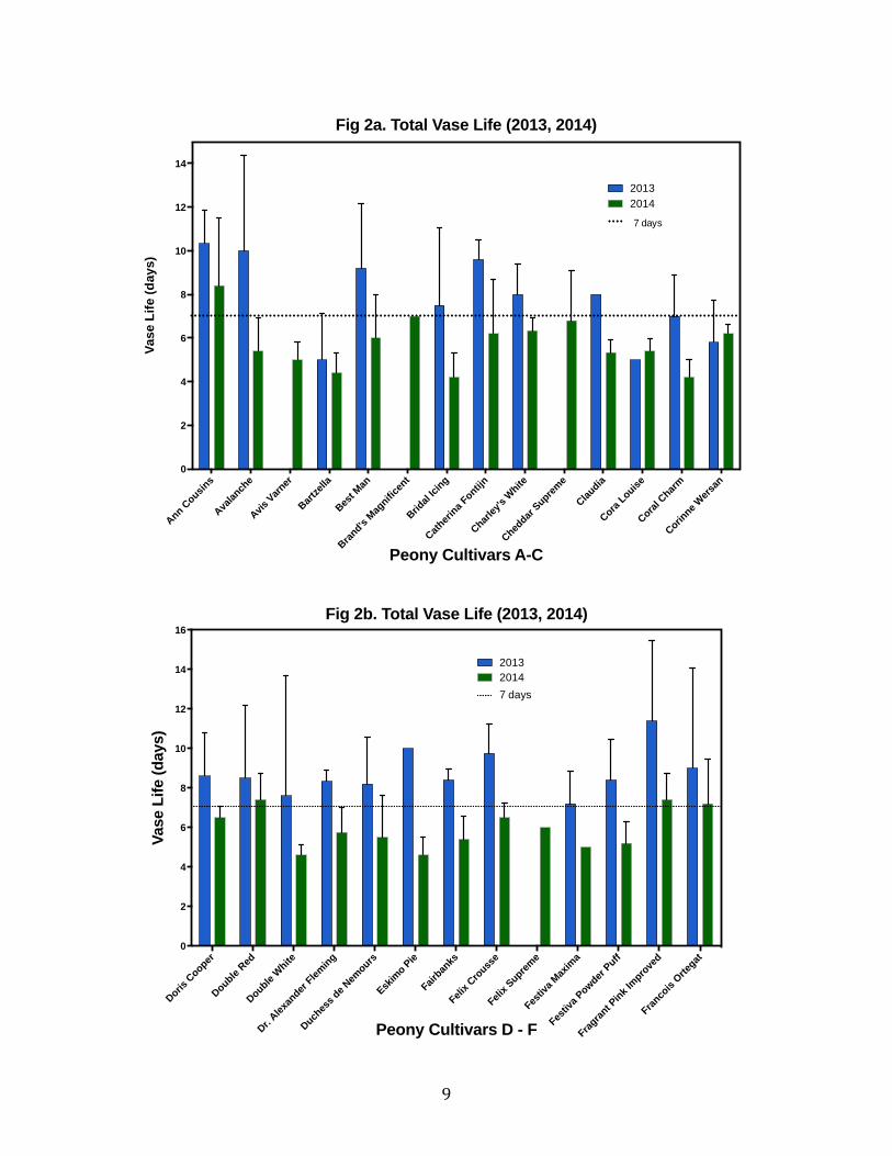
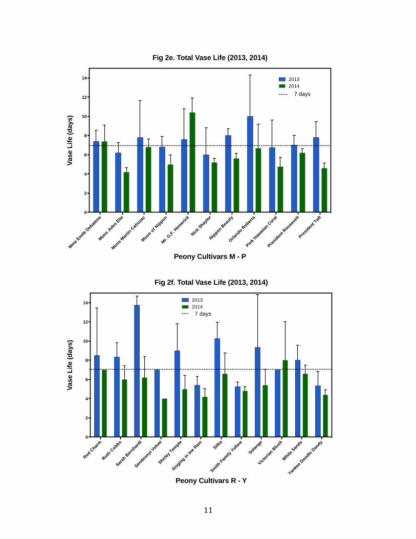
     Experiment  3.    Of  the  110  cultivars  at  the  UAF  Georgeson  Botanical  Garden,  68  cultivars  produced  sufficient  flowers  for  vase  life  analysis  in  2013  and  2014.  Vase  life  for  all  cultivars  in  2014  ranged  from  4  days  to  9  days  (mean  6.0  +  1.0  days).    In  2013,  vase  life  averaged  8.6  +  2.7  days  (range  4    -­‐  14    days)  (  Figs.  2a  -­‐  f).  Not  only  was  the  average  vase  life  more  than  2  days  longer  for  flowers  in  2013,  the  variation  among  cultivars  as  reflected  in  the  standard  deviation  was  greater.  Both  cultivar  and  year  effects  were  highly  significant  (P  <  .001),  and  there  was  a  significant  interaction  between  years  and  cultivars.  These  variables  are  not  independent.  We  expected  cultivars  to  differ  significantly  in  vase  life,  but  the  difference  between  years  was  unexpected.      

Vase  life  for  2014  was  significantly  lower  for  most  cultivars  than  2013.  In  2013,  more  than  70  percent  of  the  cultivars  showed  an  average  vase  life  of  7  days  or  more.  However,  in  2014,  only  24  percent  of  the  cultivars  had  a  similar  average  vase  life  (Table  4).  In  2013,  the  four  main  classifications  of  peonies  grown  at  the  botanical  garden  (semi-­‐double,  Japanese,  bomb  and  full  double)  showed  similar  average  vase  life  ranging  from  5  days  to  17  days.  The  bomb  classification  showed  a  slightly  lower  vase  life,  but  only  three  cultivars  were  tested  as  compared  to  41  cultivars  for  full  doubles.  The  major  classification  that  showed  a  vase  life  consistently  less  than  7  days  was  the  Intersectional  hybrids.    Because  different  cold  storage  units  were  used,  the  methods  were  not  exactly  equal  for  both  testing  years.      

  9  

 

Ann Cousin

s

Avalan

che

Avis V

arner

Bartze

lla

Best M

an

Brand's

Magnifi

cent

Bridal

Icing

Cather

ina F

ontijn

Charley

's W

hite

Cheddar

Supre

me

Claudia

Cora L

ouise

Coral C

harm

Corinne W

ersa

n0

2

4

6

8

10

12

14

Peony Cultivars A-C

Vas

e L

ife (d

ays)

Fig 2a. Total Vase Life (2013, 2014)

20132014

7 days

Doris C

ooper

Double Red

Double W

hite

Dr. Alex

ander

Flem

ing

Duches

s de N

emours

Eskim

o Pie

Fairban

ks

Felix C

rouss

e

Felix S

uprem

e

Festiv

a Max

ima

Festiv

a Powder

Puff

Fragra

nt Pin

k Im

prove

d

Franco

is Orte

gat0

2

4

6

8

10

12

14

16

Peony Cultivars D - F

Vase

Life

(day

s)

Fig 2b. Total Vase Life (2013, 2014)

201320147 days

  10  

 

Gay P

aree

Georg

e W. P

eyto

n

Glory

Hall

elujah

Going B

anan

asHeid

i

Helen H

ayes

Herm

ione

Irwin

Altm

anJo

ker

Julia

Rose

La Lorra

ine

Lady A

lexan

dra D

uff0

2

4

6

8

10

12

14

16

18

20

Peony Cultivars G - L

Vase

Life

(day

s)

Fig 2c. Total Vase Life (2013, 2014)

20132014

7 days

Lady K

ate

Largo

Leslie

Pec

k

Lillian

Wild

Lora D

exheim

er

Lottie D

awso

n Rea

Love's

Touch

Lowell T

homas

Magica

l Mys

tery

Tour

Mariet

ta S

isson

Mary B

rand

Mary J

o Legar

e

Mme de V

ernev

ille0

2

4

6

8

10

12

14

Vase

Life

(day

s)

Fig 2d. Total Vase Life (2013, 2014)

20132014

7 days

Peony Cultivars L - M

  11  

 

Mme E

mile

Deb

aten

e

Mons Jules

Elie

Mons Mar

tin C

ahuza

c

Moon of N

ippon

Mr. G.F. H

emer

ick

Nick S

haylor

Nippon B

eauty

Orlando R

oberts

Pink H

awaii

an C

oral

Presid

ent R

ooseve

lt

Presid

ent T

aft

0

2

4

6

8

10

12

14

Fig 2e. Total Vase Life (2013, 2014)

Peony Cultivars M - P

Vase

Life

(day

s)20132014

7 days

Red C

harm

Ruth C

obbs

Sarah

Ber

nhardt

Sereb

renyi

Velvet

Shirley

Tem

ple

Singin

g in tn

e Rain

Sitka

Smith

Fam

ily Y

ellow

Solange

Victoria

n Blu

sh

White

San

ds

Yanke

e Doodle

Dandy

0

2

4

6

8

10

12

14

Fig 2f. Total Vase Life (2013, 2014)

Peony Cultivars R - Y

Vase

Life

(day

s)

201320147 days

  12  

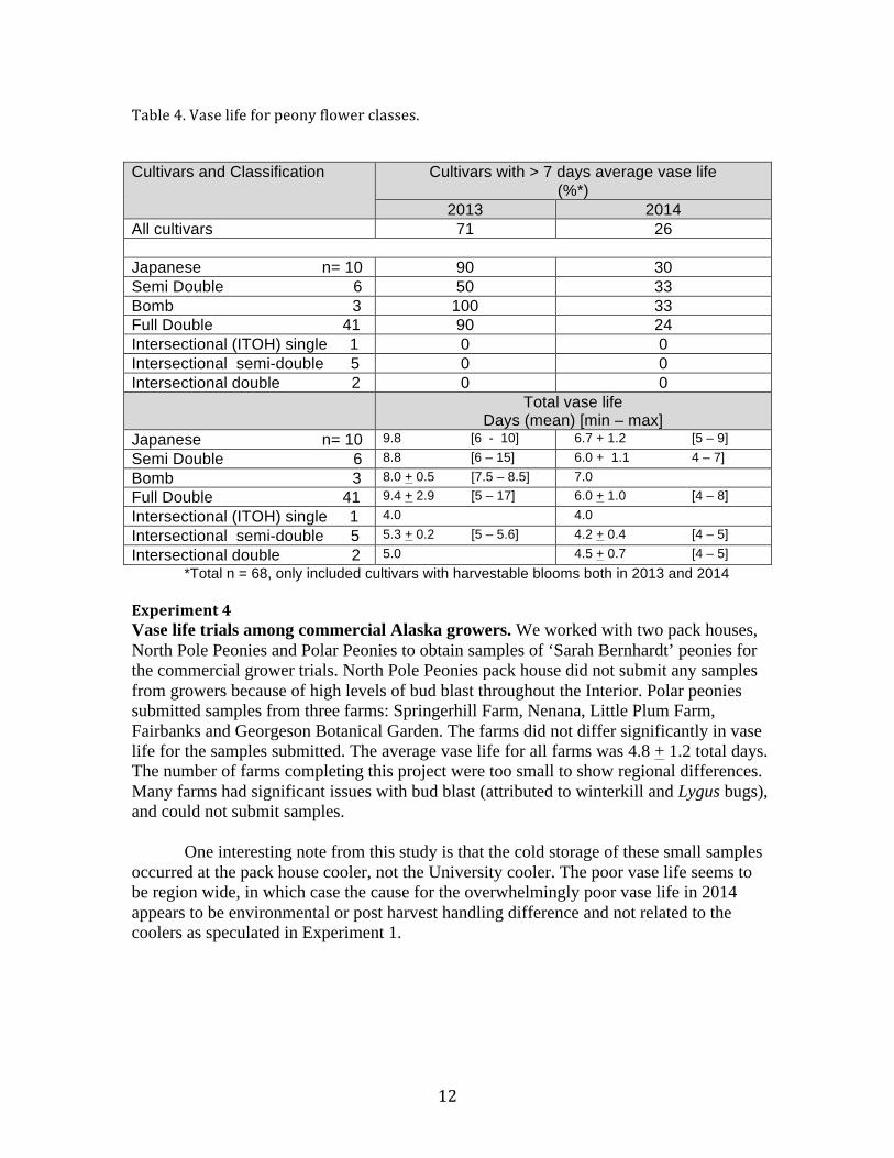
Table  4.  Vase  life  for  peony  flower  classes.    

 Cultivars and Classification Cultivars with > 7 days average vase life

(%*) 2013 2014

All cultivars 71 26 Japanese n= 10 90 30 Semi Double 6 50 33 Bomb 3 100 33 Full Double 41 90 24 Intersectional (ITOH) single 1 0 0 Intersectional semi-double 5 0 0 Intersectional double 2 0 0 Total vase life

Days (mean) [min – max] Japanese n= 10 9.8 [6 - 10] 6.7 + 1.2 [5 – 9]

Semi Double 6 8.8 [6 – 15] 6.0 + 1.1 4 – 7]

Bomb 3 8.0 + 0.5 [7.5 – 8.5] 7.0 Full Double 41 9.4 + 2.9 [5 – 17] 6.0 + 1.0 [4 – 8]

Intersectional (ITOH) single 1 4.0 4.0

Intersectional semi-double 5 5.3 + 0.2 [5 – 5.6] 4.2 + 0.4 [4 – 5]

Intersectional double 2 5.0 4.5 + 0.7 [4 – 5] *Total n = 68, only included cultivars with harvestable blooms both in 2013 and 2014

 Experiment  4  Vase life trials among commercial Alaska growers. We worked with two pack houses, North Pole Peonies and Polar Peonies to obtain samples of ‘Sarah Bernhardt’ peonies for the commercial grower trials. North Pole Peonies pack house did not submit any samples from growers because of high levels of bud blast throughout the Interior. Polar peonies submitted samples from three farms: Springerhill Farm, Nenana, Little Plum Farm, Fairbanks and Georgeson Botanical Garden. The farms did not differ significantly in vase life for the samples submitted. The average vase life for all farms was 4.8 + 1.2 total days. The number of farms completing this project were too small to show regional differences. Many farms had significant issues with bud blast (attributed to winterkill and Lygus bugs), and could not submit samples.

One interesting note from this study is that the cold storage of these small samples occurred at the pack house cooler, not the University cooler. The poor vase life seems to be region wide, in which case the cause for the overwhelmingly poor vase life in 2014 appears to be environmental or post harvest handling difference and not related to the coolers as speculated in Experiment 1.    

  13  

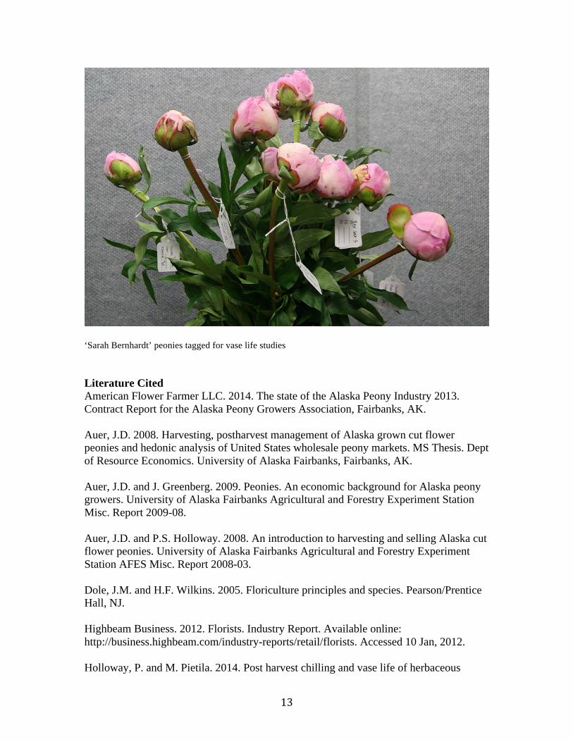
‘Sarah Bernhardt’ peonies tagged for vase life studies Literature Cited American Flower Farmer LLC. 2014. The state of the Alaska Peony Industry 2013. Contract Report for the Alaska Peony Growers Association, Fairbanks, AK. Auer, J.D. 2008. Harvesting, postharvest management of Alaska grown cut flower peonies and hedonic analysis of United States wholesale peony markets. MS Thesis. Dept of Resource Economics. University of Alaska Fairbanks, Fairbanks, AK. Auer, J.D. and J. Greenberg. 2009. Peonies. An economic background for Alaska peony growers. University of Alaska Fairbanks Agricultural and Forestry Experiment Station Misc. Report 2009-08. Auer, J.D. and P.S. Holloway. 2008. An introduction to harvesting and selling Alaska cut flower peonies. University of Alaska Fairbanks Agricultural and Forestry Experiment Station AFES Misc. Report 2008-03. Dole, J.M. and H.F. Wilkins. 2005. Floriculture principles and species. Pearson/Prentice Hall, NJ. Highbeam Business. 2012. Florists. Industry Report. Available online: http://business.highbeam.com/industry-reports/retail/florists. Accessed 10 Jan, 2012. Holloway, P. and M. Pietila. 2014. Post harvest chilling and vase life of herbaceous

 

 

  14  

peonies. Poster Presentation, American Society for Horticultural Sciences Conference, Aug 2014. Orlando, FL. Holloway, P. 2013. Cultivar trials. Available online: www.georgesonbg.org/ research/peonies/Peonycultivartrials/Cultivartrials.html. Accessed 6 June 2013. Holloway, P.S. & K.R. Buchholz 2013. The state of the Alaska peony industry. University of Alaska Fairbanks. AFES Misc.Pub. 2013-03. Holloway, P. and J. Hanscom. 2007. Peonies as field grown cut flowers for Alaska. HortScience 42(4):1016 (abstr). Holloway, P.S., J.T. Hanscom, and G.E.M. Matheke. 2003. Peonies for field cut flower production. First year growth. University of Alaska Agricultural and Forestry Experiment Station Res. Prog. Rpt. 41. Holloway, P.S., J.T. Hanscom, and G.E.M. Matheke. 2004. Peonies for field cut flower production. Second year growth. University of Alaska Agricultural and Forestry Experiment Station Res. Prog. Rpt. 43. Holloway, P.S., J.T. Hanscom, and G.E.M. Matheke. 2005. Peonies for field cut flower production. University of Alaska Agricultural and Forestry Experiment Station Res. Prog. Rpt. 44. Holloway, P.S., S. Pearce and J. Hanscom. 2010. Peony Research 2009. University of Alaska Fairbanks Agricultural and Forestry Experiment Station Misc. Pub. 2010-02. Klingman, M.A. 2002. Production and transportation considerations in the export of peonies from Fairbanks, Alaska. University of Alaska Agricultural and Forestry Experiment Station Senior Thesis ST 2005-01. Sarkar, S. 2012. Global floriculture industry trends and prospects. Floriculture Today. Available online: http://floriculturetoday.in/Global-Floriculture-Industry-Trends-and- Prospects.html. Accessed: 21 Jan 2012. United States Department of Agriculture (USDA). 2013. Floriculture.Agricultural Marketing Resource Center. Available online:www.agmrc.org/ commodities__products/specialty_crops/floriculture/Accessed Mar.10, 2013.

  15  

Postharvest Handling Methods for Enhanced Competitiveness of Fresh Cut Peonies Part 2. Effect of Boron and Calcium Sprays on Stem Strength of Peonies

Mingchu Zhang and Robert Van Veldhuizen

Introduction

The peony flower produced in Alaska is large in size. As such, the stem strength of the harvested cut flower can affect the vase life of peony. Research conducted in Chile show that spraying a calcium (10%) and boron based solution to peony cut flowers prior to harvest can increase stem strength (measured as curvature), stem weight and increase in vase time (Nelson et al., 2012). In China, spraying 4% calcium on herbaceous peony shows an increase in mechanical strength (Li et al., 2012). This enhanced mechanical stem strength probably is gained through an increase of the fraction of cell wall, endogenous calcium and pectin concentration. To increase Alaska peony competitiveness in the market, it is necessary to know if a calcium based or calcium and boron based spray solution prior to harvest can increase the postharvest quality of the Alaska peony flower.

Herbaceous peonies have a short growing season in Alaska (about 3 months). As such, they have a fast growth rate of the above ground biomass. In addition, the relative humidity in Alaska is low, indicating that a spray solution can be evaporated quickly before it is imbibed by the stems after spraying. Therefore, the designed solution for spraying should have a relatively longer residence time on the plant tissue to allow for more complete imbibition. Also, considering the availability of water in the rural communities, well water should be also taken into consideration. The objectives of the research was to 1) develop an optimal solution for a spray; 2) determine the stem diameter and strength as affected by the spray; and 3) determine the calcium and boron uptake by stems after spraying.

Methods and materials

A laboratory experiment was conducted in the Soils Laboratory of SNRE, UAF. A variety of chemicals were evaluated for their suitability as a spray agent. Two criteria were used for evaluation, 1) the solution should contain an organic compound so that it can have a prolonged resident time on tissue surface, and 2) the pH should not be extreme, either acidic or alkaline. After selecting the appropriate chemical compounds, the final spray solutions contained 5% Ca + 0.5% B + 0.1% K and 10% Ca + 0.5% B + 0.1% K. Both solutions had an approximate pH around pH 6.

A field experiment was conducted by spraying the solutions in the AFES research peony field mixed up in well water and in distilled water, respectively. The spray treatments were: 1) 5% Ca + 0.5% B + 0.1% K in distilled water, 2) 5% Ca + 0.5% B + 0.1% K in well water, 3) 10% Ca + 0.5% B + 0.1% K in well water, 4) 10% Ca + 0.5% B + 0.1% K in distilled water, and 5) no spray (control). Each treatment consisted of 32 plants, with the test cultivar being ‘Sarah Bernhardt’. Two sprayings were

  16  

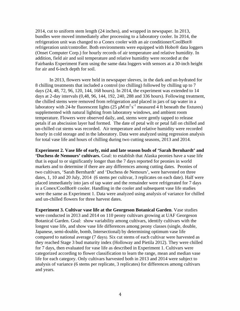
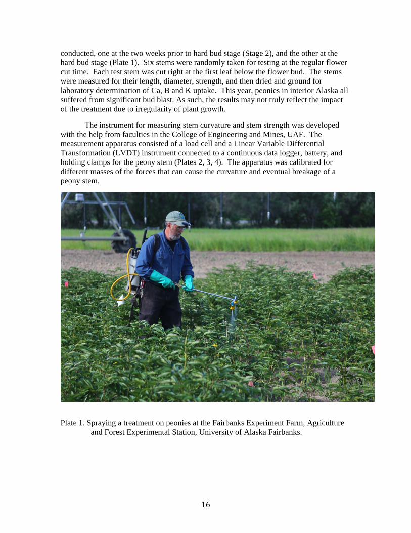
conducted, one at the two weeks prior to hard bud stage (Stage 2), and the other at the hard bud stage (Plate 1). Six stems were randomly taken for testing at the regular flower cut time. Each test stem was cut right at the first leaf below the flower bud. The stems were measured for their length, diameter, strength, and then dried and ground for laboratory determination of Ca, B and K uptake. This year, peonies in interior Alaska all suffered from significant bud blast. As such, the results may not truly reflect the impact of the treatment due to irregularity of plant growth.

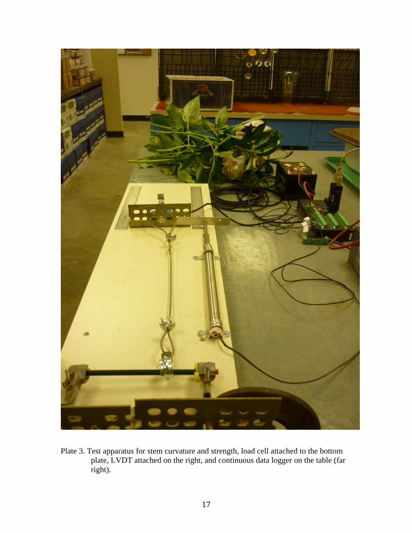
The instrument for measuring stem curvature and stem strength was developed with the help from faculties in the College of Engineering and Mines, UAF. The measurement apparatus consisted of a load cell and a Linear Variable Differential Transformation (LVDT) instrument connected to a continuous data logger, battery, and holding clamps for the peony stem (Plates 2, 3, 4). The apparatus was calibrated for different masses of the forces that can cause the curvature and eventual breakage of a peony stem.

Plate 1. Spraying a treatment on peonies at the Fairbanks Experiment Farm, Agriculture and Forest Experimental Station, University of Alaska Fairbanks.

  17  

Plate 3. Test apparatus for stem curvature and strength, load cell attached to the bottom plate, LVDT attached on the right, and continuous data logger on the table (far right).

  18  

Plate 4. Testing for stem strength and curvature.

Results

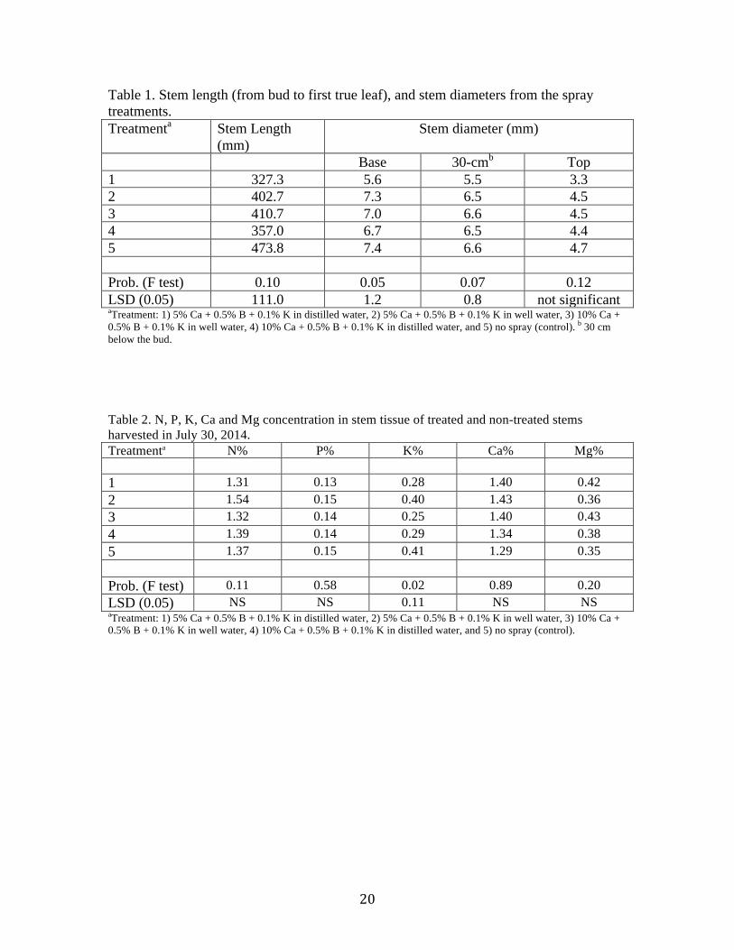
The stem diameter tended to be larger in the control treatment (Table 1). The no effect from spraying perhaps was caused by the irregular growth of the plants due to the severe bud blast this year. However, the nutrient concentration in the stem tissue showed a difference among treatments (Tables 2, 3). There was a marginal difference for potassium (K) concentration in stem tissue, but no trend can be followed (Table 2). For micronutrients, on the other hand, there was a significant difference among the treatment for boron (B), but not for calcium (Ca) (Tables 2, 3). In the spray solutions there was 10% Ca and 0.5% B. Calcium concentrations in stem tissue appeared to be not different among treatments, but the boron concentration was higher for the spray treatments than the control (no spray) (Table 3). The sources of water (well vs. distilled water) for making the solutions were not contributing to B uptake by plants (Table 3). In addition, manganese (Mn) concentration in the tissues was different among treatments (Table 3). Well water was used for Treatment 2 and 3, and distilled water was used for Treatments 1 and 4. Manganese concentration in Treatment 1 and 4 tended to be higher than that in the Treatment 2 and 3. Therefore, it seemed that source of water did have some impact on

  19  

Mn uptake. Manganese is one of the essential plant nutrients participating in many biological processes in plant (e.g. photosynthesis) (Millaleo et al., 2010). It was not clear why solution made of distilled water enhanced uptake of Mn in plant tissue.

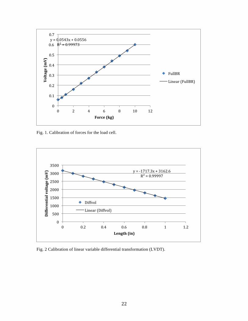
The newly assembled instrument was calibrated for the stem strength and curvature (or bending distance prior to break) test (Plate 5). The variation of forces and their corresponding voltages were correlated significantly (r2 = 0.999, p < 0.01) (Fig. 1). The variation of distances and differential voltage also correlated significantly (r2 = 1, p < 0.05) (Fig. 2). These two calibrations set up the basis for determining the force and the bending distance to break peony stems. In the stem strength test, voltage changes were recorded in the data logger connected to the load cell and LVDT instruments, and then calculated for force and distance from the regression equations in Fig. 1 and Fig. 2.

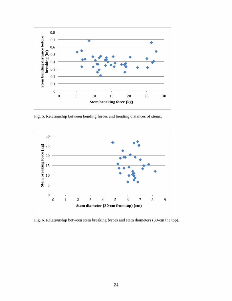
The forces required to break stems did vary from stem to stem (Fig. 3). The higher the peak in the Fig.3 indicated the larger force that was required to break the stem since there was a positive relation between the voltage and force (Fig. 1). However, the corresponding bending distance prior to breaking appeared to have less variation compared to the force (Fig. 4). There was a negative relation between the distance and voltage, therefore, the shorter the peak the longer the distance prior to breaking. It appeared that there was no relation between the amount of force required to break stems and the bending distance at stem breaking (Fig. 5). Scatter plots showed that the relations between stem diameters and stem breaking force (Fig. 6) and between stem diameter and the distance (Fig. 7) were not obvious.

Weather conditions in the summer of 2014 were not favorable for peony growth. There was a prolonged cool and wet summer during the flower production period in June and July. In addition, there was an unknown variable that caused the abortion of flower buds in many peony plants. All of these can affect the absorption of sprayed solutions by peony plants. As such, peony stem diameters seemed to not positively respond to the spray treatments (Table 1). Also, the stem strength and stem diameter were not correlated. For the stem strength and bending distance determination, the challenge still existed for the device that holds the stem for the determination even after many improvements. Stems in the holding device tended to slide out if a moderate grabbing force was used. On the other hand, the stem ends being held were broken when a strong grabbing force was used. This challenge may not affect the forces to break the stems, but it certainly affected the bending distance prior to stem breaking. Future improvements are needed for a more accurate determination of bending distance.

In conclusion, peony absorbed B but not Ca and K from the solutions sprayed on peony plants prior to flower cut, indicating spraying might be an effective way for applying B to peony plants. The spray solutions didn’t affect the stem diameter in 2014, which might be caused by abnormal weather in the summer of 2014 or the unknown variable that caused abortion of peony flowers. Therefore, to verify the impact of the spray solution on stem strength, further evaluation on the impact of sprayed solution on peonies is needed. The newly developed device can detect the forces required to break peony stems, but still fell in short to accurately determine the bending distance prior to stem breaking. Further improvements are needed to make the holding device more accountable to properly hold peony stems for testing.

  20  

Table 1. Stem length (from bud to first true leaf), and stem diameters from the spray treatments. Treatmenta Stem Length

(mm) Stem diameter (mm)

Base 30-cmb Top 1 327.3 5.6 5.5 3.3 2 402.7 7.3 6.5 4.5 3 410.7 7.0 6.6 4.5 4 357.0 6.7 6.5 4.4 5 473.8 7.4 6.6 4.7 Prob. (F test) 0.10 0.05 0.07 0.12 LSD (0.05) 111.0 1.2 0.8 not significant aTreatment: 1) 5% Ca + 0.5% B + 0.1% K in distilled water, 2) 5% Ca + 0.5% B + 0.1% K in well water, 3) 10% Ca + 0.5% B + 0.1% K in well water, 4) 10% Ca + 0.5% B + 0.1% K in distilled water, and 5) no spray (control). b 30 cm below the bud.

Table 2. N, P, K, Ca and Mg concentration in stem tissue of treated and non-treated stems harvested in July 30, 2014. Treatmenta N% P% K% Ca% Mg% 1 1.31 0.13 0.28 1.40 0.42 2 1.54 0.15 0.40 1.43 0.36 3 1.32 0.14 0.25 1.40 0.43 4 1.39 0.14 0.29 1.34 0.38 5 1.37 0.15 0.41 1.29 0.35 Prob. (F test) 0.11 0.58 0.02 0.89 0.20 LSD (0.05) NS NS 0.11 NS NS aTreatment: 1) 5% Ca + 0.5% B + 0.1% K in distilled water, 2) 5% Ca + 0.5% B + 0.1% K in well water, 3) 10% Ca + 0.5% B + 0.1% K in well water, 4) 10% Ca + 0.5% B + 0.1% K in distilled water, and 5) no spray (control).

  21  

Table 3. Cu, Zn, Mn, Fe, Cu, and B concentration in stem tissue of treated and non-treated stems harvested in July 30, 2014. Treatmenta Cu Zn Mn Fe B ppm 1 4.33 14.17 15.92 58.27 39.15 2 4.70 15.88 12.45 43.55 39.73 3 4.42 15.03 11.60 36.30 40.75 4 4.30 14.48 14.05 58.22 50.83 5 4.40 16.27 11.67 49.25 17.63 Prob. (F test) 0.50 0.60 0.03 0.44 0.0001 LSD (0.05) NS NS 2.93 NS 11.05 aTreatment: 1) 5% Ca + 0.5% B + 0.1% K in distilled water, 2) 5% Ca + 0.5% B + 0.1% K in well water, 3) 10% Ca + 0.5% B + 0.1% K in well water, 4) 10% Ca + 0.5% B + 0.1% K in distilled water, and 5) no spray (control).

Plate 5. Peony stem was broken after imposed certain force with the force at the point of stem breaking recorded in the data logger.

  22  

Fig. 1. Calibration of forces for the load cell.

Fig. 2 Calibration of linear variable differential transformation (LVDT).

y  =  0.0543x  +  0.0556  R²  =  0.99973  

0  

0.1  

0.2  

0.3  

0.4  

0.5  

0.6  

0.7  

0   2   4   6   8   10   12  

Voltage  (mV)  

Force  (kg)  

FullBR  

Linear  (FullBR)  

y  =  -­‐1717.3x  +  3162.6  R²  =  0.99997  

0  

500  

1000  

1500  

2000  

2500  

3000  

3500  

0   0.2   0.4   0.6   0.8   1   1.2  

Differential  voltage  (m

V)  

Length  (in)  

Diffvol  

Linear  (Diffvol)  

  23  

Fig. 3. Example of test for breaking force for peony stems. The higher the peak, the larger the force is required to break the stem.

Fig. 4. Example of test for bending distance from which stem was broken. The lower the peak, the more the bending of stem can bear.

-­‐0.2  

0  

0.2  

0.4  

0.6  

0.8  

1  

1.2  

1.4  

1.6  

10001  

10043  

10085  

10127  

10169  

10211  

10253  

10295  

10337  

10379  

10421  

10463  

10505  

10547  

10589  

10631  

10673  

10715  

10757  

10799  

10841  

10883  

10925  

10967  

Force  in  mVoltage  

Test  sequence  (second)  

-­‐6000  

-­‐5000  

-­‐4000  

-­‐3000  

-­‐2000  

-­‐1000  

0  

1000  

2000  

3000  

4000  

10001  

10043  

10085  

10127  

10169  

10211  

10253  

10295  

10337  

10379  

10421  

10463  

10505  

10547  

10589  

10631  

10673  

10715  

10757  

10799  

10841  

10883  

10925  

10967  

Differential  voltage  for  length  

Test  sequence  (second)  

  24  

Fig. 5. Relationship between bending forces and bending distances of stems.

Fig. 6. Relationship between stem breaking forces and stem diameters (30-cm the top).

0  

0.1  

0.2  

0.3  

0.4  

0.5  

0.6  

0.7  

0.8  

0   5   10   15   20   25   30  

Stem

 bending  distance  before  

breaking  (in)  

Stem  breaking  force  (kg)  

0  

5  

10  

15  

20  

25  

30  

0   1   2   3   4   5   6   7   8   9  

Stem

 breaking  force  (kg)  

Stem  diameter  (30-­‐cm  from  top)  (cm)  

  25  

Fig. 7. Relationship between stem bending distances before breaking and stem diameters (30-cm from top).

References

Li, C., J. Tao, D. Zhao, C. You, and J. Ge. 2012. Effect of calcium sprays on mechanical strength and cell wall fractions of herbaceous peony (Paeonia lactiflora Pall.) inflorescence stems. In. J. Mol. Sci. 13:4704-4713.

Loyola-Lopez, N., C. Prieto-Labbe, and B. Villouta-Barr. 2012. Application calcium, boron and sucrose on cut peony (Paeonia lactiflora Pall.) c. Karl Rosenfield. Agronomia Colombiana, 30:103-110.

R. Millaleo, R., M. Reyes-Díaz, A.G. Ivanov, M.L. Mora, and M. Alberdi. 2010. Manganese as essential and toxic element for plants: transport, accumulation and resistance mechanisms. J. Soil Sci. Plant Nutr. 10: 476 – 494.

0  

0.1  

0.2  

0.3  

0.4  

0.5  

0.6  

0.7  

0.8  

0   1   2   3   4   5   6   7   8   9  

Stem

 bending  distance  (in)  before  

breaking  

Stem  diamter  (30-­‐cm  from  top)(cm)