This item was submitted to Loughborough's Research Repository by the author. Items in Figshare are protected by copyright, with all rights reserved, unless otherwise indicated.

Post-crisis macrofinancial modeling: Continuous time approachesPost-crisis macrofinancial modeling: Continuous time approaches

PLEASE CITE THE PUBLISHED VERSION

https://www.palgrave.com/gb/book/9781137494481

PUBLISHER

© Palgrave Macmillan

VERSION

AM (Accepted Manuscript)

PUBLISHER STATEMENT

This work is made available according to the conditions of the Creative Commons Attribution-NonCommercial-NoDerivatives 4.0 International (CC BY-NC-ND 4.0) licence. Full details of this licence are available at:https://creativecommons.org/licenses/by-nc-nd/4.0/

LICENCE

CC BY-NC-ND 4.0

REPOSITORY RECORD

Isohaetaelae, Jukka, Nataliya Klimenko, and Alistair Milne. 2019. “Post-crisis Macrofinancial Modeling:Continuous Time Approaches”. figshare. https://hdl.handle.net/2134/20551.

Post-crisis macrofinancial modelling: continuoustime approaches

Chapter for "Handbook of Post-Crisis Financial Modelling" ∗

Jukka Isohätälä, Nataliya Klimenko and Alistair Milne

April, 2015

1 IntroductionPrior to the crisis the dominant paradigm in macroeconomic modelling was

the micro-founded ‘New-Keynesian’ DSGE model (described in many textbooksincluding the influential exposition of Woodford [2003]). In its most basic formthis combines price-stickiness with forward looking decision making by bothhouseholds and firms. This provides a tractable framework for capturing theresponse of output and inflation to both demand and supply shocks and ex-plaining intuitively the transmission of monetary policy (with monetary policycharacterized as a choice over rules for current and future interest rates).

DSGE models have proved to be remarkably adaptable, being easily ex-tended in many ways, most commonly by incorporating the so called ‘financialaccelerator’, a premium on the cost of external investment finance decreasing infirm net worth (Bernanke et al. [1999]) and hence creating an extended dynamicresponse to shocks. DSGE models could also be fitted closely to macroeconomicdata, successfully capturing macroeconomic fluctuations observed over severalpast decades (as demonstrated by Smets and Wouters [2005]).

Despite these successes the crisis revealed fundamental weaknesses in thisDSGE paradigm. DSGE models proved incapable of explaining the protracteddecline in output and investment in the industrial countries following the crisisof 2008 (or similarly persistent declines following other previous financial crisesas documented by Reinhart and Rogoff [2009]). Contrary to widespread percep-tion, DSGE models can be relatively easily extended to incorporate banks andbank balance sheets.1 However, even with banking and other financial frictions,DSGE models, in their usual linearised form, fail to reproduce the sudden, sub-stantial and long-lasting changes in asset prices, output or investment inherentin the periods of financial crises including that of 2008.

∗We are grateful for comments from Marcus Brunnermeier and from the handbook editors1An example of such a DSGE extension is Meh and Moran [2010] who generalise the

financial accelerator to include a bank-moral hazard based on Holmstrom and Tirole [1997].

1

The objective of this chapter is to introduce an emerging literature, pursuedsince the financial crisis, employing non-linear continuous time specifications ofeconomic dynamics to capture the possibility of marked and sometimes longlasting changes in financial asset prices and asset price volatility or in real econ-omy aggregates such as output or investment.2 Prominent contributions to thisnew literature include He and Krishnamurthy [2012] and Brunnermeier and San-nikov [2014b]. We aim to explain the methods used in this new literature anddemonstrate how they can be applied to a range of different modelling problems.This is however not a complete review of the literature on macroeconomics withfinancial frictions (Brunnermeier et al. [2012] provides more extended reviewthan we do, discussing a wider range of macroeconomic consequences of marketincompleteness with extensive references to prior literature). Our aim is morelimited, providing a fairly full discussion of what we perceive as some of the keycontributions and describing both the economic intuition and technical solutionmethods that underpins their results.

This new approach to macroeconomic modelling is still very much in its in-fancy and the specifications employed in this generation of models are highlystylised. One way of describing this new literature is to say that it applies thetool of continuous-time modelling widely used for derivative and other assetpricing problem to a new class of macroeconomic general equilibrium problems.This though is a bit of an oversimplification – the standard financial applicationsof continuous time modelling beginning with Merton [1969, 1971] and Black andScholes [1973] all assume complete markets. By contrast, the key underlyingassumption of this new literature is market incompleteness – not all risks can becostlessly traded. The reasons for this market incompleteness are not typicallyhowever modelled. Instead, the focus is on the implications of market incom-pleteness for aggregate macrodynamics and in particular the macrodynamic roleof balance sheet structure (the net worth and leverage of households, companiesand financial intermediaries).

Market incompleteness can also be modelled in a discrete time setting, sowhy employ continuous time? The reason is that specifying the dynamics of theeconomy in continuous time, using diffusion processes governed by stochasticdifferential equations or sometimes jump processes, allows for a convenient de-scription of the fully non-linear macrodynamics. The possible realisations of theeconomy are characterised by a set of differential equations3 and the solutionof these equations, subject to appropriate boundary conditions, yielding boththe macroeconomic outcomes (as a function of state) and the probabilities ofthese outcomes occurring (that is, the ‘ergodic’ density or the probability den-sity function of the state variable). Knowledge of the probability distributionof states then allows the analysis of the full macroeconomic dynamics. In themodels reviewed in this chapter this approach is used to characterise both the

2Our paper complements Brunnermeier and Sannikov who provide a detailed discussion ofthe solution methods employed in these continuous-time models of this kind.

3Generally, these are partial differential equations, but when the model in question hasjust a single state variable, as is the case in the models we review here, the equations becomeordinary differential equations.

2

impact and persistence of fundamental shocks and how this can reproduce somecharacteristic crisis features.

A key determining feature of the properties of this new generation of macroe-conomic models is the magnitude of shocks relative to the balance sheet con-straints that arise because of market incompleteness. If these shocks are rela-tively small, the model dynamics are dominated by the deterministic compo-nents of equations of state motion (e.g., the planned or expected saving andinvestment) and the diffusion of state towards these net worth or leverage con-straints occurs only rarely so that model predictions are not so very differentfrom those of conventional macroeconomic models. In this case linearised mod-els of the kind employed in the DSGE tradition can adequately approximate thefully non-linear solution.

However, if shocks are sufficiently large so that stochastic disturbance canon occasion become much more important than the deterministic componentsof state motion and net worth or leverage are pushed towards constrained levelsrelatively frequently, then qualitative changes in model predictions are possible.Agents (households, firms, governments) substantially alter their behaviour, notjust when the constraints are actually binding but when they are close to bind-ing and sometimes even quite far away from these constraints. They do so inorder to self-insure, offsetting the absence of markets that they would like touse to protect themselves against risk. This collective attempt to avoid riskcan then in turn create feedbacks at the macroeconomic level following a largedisturbance. The latter induce additional volatility of asset prices encouragingeven greater self-insurance and inefficient employment of real economic resources(amplification) that potentially trigger long lasting declines of real macroeco-nomic aggregates (persistence) such as output, employment and investment.

In these circumstances DSGE-based linearisation can no longer provide anadequate description of aggregate dynamics, as this requires explicit modelling ofinduced volatility rather than the trend. Note though that there is no necessaryand direct relationship between the magnitude of shocks and the frequency ofsuch crisis episodes. In many of these specifications a relatively small exogenousnoise may cause agents to operate with relatively small buffers of net worth,in which case even comparatively small disturbances can result in substantialdepartures from the predictions of linearised macroeconomic models (this a keyfinding of Isohätälä et al. [2014b] and seems to be what underlies the ‘paradoxof volatility’ described, for example, by Brunnermeier and Sannikov [2014b]).

This chapter contains three main sections and provides detailed discussionof six contributions to the literature. Section 2 provides a general overview ofthis new literature, discussing how a combination of specific economic assump-tions and modelling strategy generates results which differ sharply from moreestablished traditions of macrodynamic modelling. Section 3 reviews a numberof recent applications, some journal published, others work of our own still atworking paper stage. This section is itself divided into a number of subsections:3.1 focuses on the continuous time modelling of the dynamics of asset prices,following the approach taken by He and Krishnamurthy [2012] and also a relatedproblem of optimal savings and consumption in general equilibrium addressed

3

by Isohätälä et al. [2014a]; 3.2 then discusses the dynamic modelling of the in-teraction of sectoral balance sheets with production and investment, focusingon the work of Brunnermeier and Sannikov [2014b] and the closely related par-tial equilibrium model of Isohätälä et al. [2014b]; 3.3 then discusses the furtherextension of these models to an explicit treatment of financial intermediation,describing current work by Klimenko et al. [2015] and Brunnermeier and San-nikov [2014e]. Section 4 offers an illustrative example of the required solutionmethods in the context of a simple model, a simplification of Brunnermeier andSannikov [2014b]. This section is supported by a technical appendix providinga heuristic outline of solution methods. Section 5 then discusses the substan-tial agenda for future research opened up by this new ‘post-crisis’ approach tomacro-financial modelling. Section 6 concludes.

2 Strengths and weaknesses of the new literatureThis section provides a general overview of the new literature on continuous

time macrofinancial dynamics. Neither the economics nor the solution methodsemployed in this literature are in themselves especially novel. The contributioncomes from combining balance sheet restrictions, in appropriately chosen con-texts, with the tools of continuous time stochastic dynamic optimisation. Thissection therefore proceeds by outlining the economics of this new literature com-paring it with an earlier substantial body of research, dating back to the late1980s, that addresses the aggregate implications of market incompleteness. Italso offers a short discussion of the technical strengths and shortcomings of thisnew approach.

Most of this earlier work focused on the absence of markets for insuringidiosyncratic household labour income risks, a market incompleteness that canreduce the equilibrium real interest rate (Huggett [1993], Aiyagari [1994]) andprovides one potential explanation of the incompatibility of the equity marketrisk premium with complete market models of household consumption-savingsdecisions (Mankiw [1986]).4 The particular strand of this work closest to thenew macrofinancial dynamics (initiated by Krusell and Smith [1997, 1998]) con-siders the dynamics of capital accumulation in economies combining uninsurableidiosyncratic shocks to employment with aggregate shocks to the productivityof capital. As with the new continuous time macrofinancial literature there areno analytical solutions, so numerical methods must be applied. A comparisonof these two literatures offers useful insight into their respective strengths andweaknesses.

Macrodynamic analysis with incomplete markets is only ever tractable withstrong simplifying assumptions. In the presence of market incompleteness, suchas limits on individual household borrowing or frictions in access of firms tocapital markets, standard aggregation results no longer hold.5 This calls into

4See Guvenen [2011] for a detailed review of this literature.5The standard results are those of Gorman [1959], who considers restrictions on utility

under which consumption of goods can be expressed as a linear function of wealth allowing

4

question the appropriateness of widely employed ‘representative agent’ models.Full solution, based on the standard assumptions of complete information andmodel consistent expectations, requires every decision maker to track the currentstate and laws of motion of the entire distribution of assets and liabilities acrossall individual agents. There are therefore at least as many state variables asthere are agents in the economy.

The new continuous-time macrofinancial literature sidesteps this challengeof of aggregation, reintroducing the representative agent by assuming eitherthat all agents of a particular type are exactly the same, with the same tastesor technology and affected simultaneously by the same shocks (within sectorhomogeneity); or by assuming that all agents of a particular type can costlesslytrade all financial and real assets with each other (within sector market com-pleteness) with often at least some assets also traded between sectors.6 Thesestrong assumptions have allowed these models to capture qualitative changes inaggregate behaviour that arise when there is a substantial probability of bal-ance sheet constraints binding or coming close to binding, and the possibility offeedbacks that then amplify shocks and generate persistent fluctuations in eco-nomic aggregates and asset prices. They do though illustrate one of the mainpoints we draw from our review: this new literature is still immature with muchwork yet to be done to examine how well its predictions hold in more realisticsettings.

The older literature on aggregate productivity shocks and uninsurable labourincome deals with this aggregation problem in a quite different way, restrictingattention to particular model specifications in which solution can be reasonablyaccurately approximated by individual agent decision rules based on a smallnumber of summary statistics for the entire distribution of household wealth.

The influential contribution of Krusell and Smith [1997, 1998] was to solvesuch a model, with two idiosyncratic employment states (employed, unem-ployed) and two aggregate productivity states (high in boom, low in recession),using a numerical schema which enforced model consistent capital dynamics anddemonstrating that the resulting outcome exhibited ‘approximate aggregation’in the sense that increasing the number of summary statistics for the wealthdistribution used by households in their consumption/saving decisions beyonda small manageable number did not affect model outcomes.7 An entire branchof literature has emerged focused on the numerical accuracy of this and other

the choices of a large number of households to be restated as that of a representative consumer;and of Rubinstein [1974] and Constantinides [1982] who examine aggregation in the context ofportfolio allocation-consumption decisions. Constantinides [1982] shows that under relativelyweak conditions with complete financial markets the decisions of individual consumers can bereplaced by that of a composite representative agent. See Guvenen [2011] for more discussion.

6Similarly strong representative agent assumptions are also imposed in earlier literatureon the macroeconomics of financial frictions, including in the influential work of Kiyotaki andMoore [1997] and Bernanke et al. [1999].

7The Krusell-Smith algorithm for obtaining model consistent capital dynamics is based onupdating a linear rule for the period by period investment in the stock of capital through aregression on the simulated model output from the previous iteration, iteration is continueduntil the investment rule is model consistent and the accuracy of the numerical solution isjudged by the fit of the regression.

5

alternative algorithms for solving models of this kind (for further discussion seeAlgan et al. [2010], Den Haan [2010]).

A weakness of the Krusell-Smith algorithm is its model dependence.8 Whileit appears to work reasonably well for particular calibrations of the specificmodel for which it was developed, it is far from clear that it can provide areliable approximation to the dynamics of the kind that emerge in the new con-tinuous time macrofinancial models we review. One limitation is that it makesno allowance for the resulting dynamic changes in interest rates or other financialasset prices consequent on changes to individual agent balance sheets. Anotherlimitation is that there is no guarantee against the algorithm converging on a‘wrong’ outcome in which the particular model simulations generated at con-vergence contain insufficient examples of the balance sheet constraints leadingto qualitative shifts in the decisions of households or other agents that in turnsubstantially influence macroeconomic dynamics.9

Another obvious difference is that the earlier literature on macroeconomicdynamics in the presence of market incompleteness follows the dominant prac-tice in macroeconomic modelling of assuming that time is discrete rather thancontinuous. The choice between discrete and continuous time is, however, lessimportant than might at first appear. It can admittedly be a barrier to under-standing.10 But numerical solution using a computer always eventually requiresdiscretization. Our view is that these two assumptions (discrete vs continuous)are complementary, each with their own strengths and weaknesses. It shouldbe possible to state any of these models using either approach, and the choicethen comes down to which is more convenient for solution and communicationof results.

Continuous time diffusion has some advantages. Provided that the modelcan be specified with a small number of heterogeneous agents, tractable solutioncan be computed using ordinary or partial different equations sidestepping con-cerns about the existence of a ‘Markovian’ equilibrium. Another conveniencethat all paths are continuous so there is no need to be concerned about thepossibility of assets or liabilities jumping beyond constrained values.11 Solutionvia ordinary or partial differential equations provides an efficient way of captur-

8For further discussion see Den Haan [2010].9Another way of thinking about these challenges of numerical convergence is that an algo-

rithm of this kind in effect substitutes moments of the distribution of networth, both acrossindividual agents and across time, for the full distribution. If insufficient moments are includedthen the algorithm may yield a poor approximation to the correct solution.

10In Section 4 of this chapter we discuss the technicalities of solution of a simple illustra-tive example of continuous time macrofinancial modelling, hoping in this way to make thisliterature accessible to readers who are much more familiar with discrete time modelling. Wealso recommend as good practice further steps to assist readers become acquainted with thesemethods. One helpful presentational device, used for example by Klimenko et al. [2015], is tofirst state a model in discrete time with time steps of length ∆t and then derive the limit as∆t→ 0. Another helpful step is to develop standalone numerical solvers which allow readersto use ‘sliders’ to vary parameters and observe the consequent changes in solutions. The web-site www.leveragecycles.lboro.ac.uk contains examples of such standalone solution softwarefor two of the papers reviewed here, Isohätälä et al. [2014b] and Isohätälä et al. [2014a].

11This, however, does not apply to jump-diffusion processes.

6

ing the impact across the state space of constraints on behaviour at or close toboundaries. As discussed in the next section, specification in continuous timealso allows the application of the convenient method of asymptotic expansionin order to capture the singularities that can emerge when financial constraintsare hit. Finally, specification in continuous time with diffusion also means thatdecision rules can be expressed in relatively simple terms, namely, as functionsof derivatives or partial derivatives of the value function (i.e., marginal values),thereby, providing useful economic intuition that is not so easily obtainable indiscrete time.

Discrete time has the advantage that solution can be computed using the welldeveloped and widely used tools of backward recursion. The literature offers awell developed discussion of both the existence and computation of equilibria indiscrete time, including for macroeconomic models with incomplete markets.12There are larger amounts of available software developed for solution of discretetime models. Solution methods are now well understood both when distur-bances are relatively small compared potential constraints so linearisation canbe employed and for many non-linear models including several state variables(dynamic stochastic macroeconomic models can now be routinely solved withfour or more states). Some forms of lagged response – e.g. the policy responselags resulting from delays in the release of statistical information are more nat-urally specified in discrete time.

So far our comparison of these two literatures has focused on the technicalchallenges of aggregation and numerical solution. Comparison of these two liter-atures also highlights some differences in economic assumptions. One is that inolder literature, for example Krusell and Smith [1998], it is individual householdswho are financially constrained, whereas in Brunnermeier and Sannikov [2014b]it is the representative firm that is financially constrained (as we describe belowin Section 3, they are unable to borrow more than the market value of their cap-ital). Krusell and Smith [1998] find that these underlying financial constraintsmake relatively little difference to aggregate dynamics, whereas Brunnermeierand Sannikov [2014b] find that the constraints substantially reduce output andinvestment when firm net worth (as a proportion of the market value of theeconomy’s capital stock) falls close to zero.

But perhaps the most important advantage of the radical simplifying as-sumptions made in the continuous-time macrofinancial literature is the wide

12See Krueger and Kubler [2008] for a short overview, including discussion of the challenge ofcomputing solution in a small number of state variables when it is no longer possible to obtainsolution using contraction mapping theorems (theorems closely related to the aggregationresults of Constantinides [1982] and the implied correspondence between market equilibriumand an equivalent central planning problem). The algorithm of Krusell and Smith [1998] isthe most widely cited example of such methods applied in the context of incomplete markets.Ljungqvist and Sargent [2000] chapter 17 offers a number of other examples of solution forincomplete market economies and FENG et al. [2014] and Guerrieri and Iacoviello [2015] fortwo recent proposed methods for recursive numerical solution of incomplete market models indiscrete time. Tractable solutions of these models are described as ‘Markovian’ because thestochastic dynamics can be expressed in terms of the equations of motion of a limited numberof state variables.

7

range of issues that can then be addressed. This will become clearer fromour review of individual models in the next section that explore the impact ofconstraints on households, firms and intermediaries for the dynamics of assetprices, output and investment. As we discuss in Section 5, there is scope forconsiderable further work of this kind on the dynamic consequences of marketincompleteness for a range of other aggregate economic variables, including em-ployment, price setting, government finances and macroeconomic policy. Theprice paid for these advances is not insubstantial, a clear data discrepancy atthe microeconomic level since not all firms or all households are able to tradeamongst each other to achieve common ratios of debt to assets (i.e. the as-sumption that each sector can be replaced by a single representative agent isnot a realistic assumption in the context of incomplete markets). This thoughpurchases valuable new understanding of a range of macroeconomic phenomenathat are attracting attention in the wake of the global financial crisis.

3 A review of some recent continuous-time macro-financial models

In this section we review some recent continuous-time macrofinancial models.Our discussion covers three prominent papers that have attracted widespreadattention together with three papers of our own. It is organized as follows.Section 3.1 discusses how continuous time models have been used to modelthe dynamics of assets prices, including the return on risk-free assets and thepremium on risky assets. 3.2 reviews implications of the dynamic allocationof productive capital for financial stability. Section 3.3 discusses extensions ofthese models to the explicit treatment of the banking sector.

3.1 Capital constraints and asset pricingThe series of papers developed by He and Krishnamurthy [2012, 2013] (here-

after, HK(2012) and HK(2013)) explores how market incompleteness affects therisk premium on risky assets in a Lucas Jr. [1978]-type endowment economy inwhich cash flow yields (dividends) on risky asset follow a random walk. Thekey distinguishing assumption of these models is that risky assets are held onlyby specialist financial intermediaries subject to agency frictions similar to thosemodelled in Holmstrom and Tirole [1997]. Incentive compatibility (i.e., avoid-ing the mismanagement of assets or ‘shirking’) requires that these intermediariesmust finance their investments with a minimum proportion of their own equity.When intermediary capital is scares, this equity capital constraint binds andworks as a channel of amplification of fundamental shocks to intermediary as-sets and net worth, increasing the volatility of returns and the risk premiumearned from investment in the risky asset.

Here we focus on the model developed in HK(2012) (the other model issimilar). HK(2012) model the economy in which there is a single risky, non-tradable asset of a fixed size and the market price Pt that reflects the expected

8

discounted value of dividend streams.13 The asset generates a stochastic flowof dividends Dt per unit of time, that evolves as a Geometric Brownian motionwith a constant drift and volatility σ. There exists also a risk free asset (bonds)in zero net supply and interest rate rt, i.e. there is the possibility of lendingbetween the households and specialists. The risky asset’s risk premium is thengiven by

πR,t = E[Dt dt+ dPt

Pt

]/dt− rt.

There are two classes of investors: specialists managing financial interme-diaries that play the role of investment vehicles and households who delegateinvestment decisions to specialists, as they have no direct access to investmenttechnologies (i.e., there is market segmentation). In this and all following mod-els we review in this section, all agents belonging to a particular group areidentical. Such a simplification is key for obtaining tractable solutions, as itallows working with a representative agent making the optimal decisions basedon observations of her own level of wealth and (typically) a unique aggregatestate.

Both specialists’ and households’ wealth is invested in intermediaries. Theoptimal contract between households and specialists determines βt ∈ [0, 1] – thespecialist’s share of investment in the risky asset and hence, after allowing fora fee Kt dt that may be paid to specialists for managing entrusted funds, theirclaim on dividend income. Specialists choose the total volume of investmentin the risky asset, Et, and make a working/shirking decision unobservable tohouseholds. As in Holmstrom and Tirole [1997], shirking reduces the cash-flowfrom risky assets by Xt dt but enables specialists to collect private benefits Bt dtwhich are assumed to be proportional to the reduction in the asset cash-flow,caused by shirking:

Bt dt =1

1 +mXt dt,

where the inverse of m captures the magnitude of agency frictions.14The incentive contract preventing shirking places restrictions on outside eq-

uity financing. Namely, the households’ equity stake must be limited to a frac-tion of the total risky investment that depends on the magnitude of agencyfrictions, which leads to the following equity capital constraint:

Eht ≤ mEt. (1)

Put differently, to abstain from shirking, specialists must maintain some ‘skinin the game’, whose proportion is increasing with the magnitude of agency

13By contrast, the models by Brunnermeier and Sannikov [2014b] and Brunnermeier andSannikov [2014e] that we review below enable the asset to be traded among two classes ofagents, which allows capturing the impact of “fire sales” on asset prices and track their feed-backs into the dynamics of agents’ wealth.

14A further assumption, introduced in order to avoid the challenges of solving for punish-ment and reward strategies as a dynamic game, is that the contract between households andspecialists is lasting only from t to t+ ∆t after which the relationship between household andspecialist is broken and each household is paired with a new specialist. This means that theequity constraint emerges as the solution to a static bargaining problem.

9

frictions. In terms of the sharing rule, the above constrain implies that

β∗t ≥1

1 +m, for Kt ≥ 0,

with equality when Kt > 0.To obtain a closed form solution He and Krishnamurthy [2012] assume that

both specialists and households have log-preferences over instantaneous con-sumption. With this assumption, the value function of any representative agentis additively-separable and can be written in the following form:

1

ρilog(W i

t ) + Y it ,

where ρi is the discount rate of the agent i = s, h (specialist and household,respectively), W i

t is the wealth of the agent i and Y it is the function of theaggregate wealth and dividends, which are two state variables in this setting.

Due to the above property of the value function, the portfolio and con-sumption choices of agents are almost trivial. In particular, agents continuouslyconsume an amount proportional to their net worth, where the consumptionrates are given by their respective discount factors, i.e., cit = ρiW i

t and the opti-mal exposure to risky asset is given by the mean-variance portfolio choice, yet,with a slight twist for households for whom the effective asset risk premium isreduced by the scaled intermediation fees kt = Kt/Eht .

Finding the unique equilibrium of this model requires solving for three pro-cesses – risky asset price Pt, riskless interest rate rt and scaled intermediationfees kt – compatible with the individual maximization and market clearing con-ditions. Pt, rt and kt are the functions of the unique state variable – theaggregate specialists’ wealth scaled by aggregate dividends, wt ≡W s

t /Dt.Depending on the level of the scaled specialists’ net worth, at each moment

of time the economy can find itself in one of two regimes: if scaled specialist networth wt exceeds a critical threshold wc ≡ 1/(ρhm+ ρs) then the solution is inan unconstrained regime in which the incentive constraint (1) is slack; otherwisethe solution is in a constrained regime in which the incentive constraint (1) isbinding.

In the unconstrained regime where the wealth of the specialist financial in-termediaries is relatively high, the risk premium is constant and households payzero fees for intermediation. There is no borrowing or lending (with the implicit‘risk-free’ rate of interest rt, a wealth dependent weighted average of the discountrates of households and specialists, that declines as wt increases). Holdings inthe risky asset (βt) are proportional to agent wealth. The price volatility of therisky asset is constant and is equal to the volatility of the dividend cash-flow,i.e., σR,t = σ.15

15This property emerges essentially due to the absence of leverage in the unconstrainedregion. In the models we review next, the endogenous volatility is affected by the changesin leverage/feedbacks from asset prices and does not remain constant even when the capi-tal/leverage constraints are far from binding.

10

In the constrained region, in which the wealth share of the specialist financialintermediary are relatively low (below wc), the equity constraint binds. Theirrelatively low level of wealth means that the specialists must borrow from house-holds in order to maintain their required share of holdings of the risky asset.The volatility of the risky asset (endogenous volatility),

σR,t = σ[ (1 +m)ρh

(ρhm+ ρs)(1 + (ρh − ρs)wt)

]> σ,

then drives the level of both the risk premium and of intermediation fees in theconstrained regime. These are both always higher than in the unconstrainedregime, but decreasing with the scaled specialists wealth until the threshold be-tween the two regimes is reached. The risk free interest rate (at least for thechosen parameterisations) also exhibit a different pattern than in the uncon-strained region: namely, it becomes an increasing function of specialist wealth,i.e., in the constrained regime, the lower the specialist wealth, the higher thevaluation placed on risk-free assets.

The HK(2012) model predicts that intermediaries only borrow in the con-strained regime, otherwise intermediaries are unleveraged. In order to generateleverage in the unconstrained regime and so better match the data, HK(2013)amend their earlier model by introducing household labour income uncertaintyand an exogenous demand by households for holding a minimum proportion ofwealth in the form of risk-free lending to specialists.16 Solution is now numeri-cal, not closed form. Parameters are chosen so that, absent of any constraints,the risk-tolerant households hold all their wealth in the form of risky assets andas a result the equity constraint on specialists binds approximately fifty percentof the time. With this set up the model does a fairly good job of reproducing thedynamics of risk-premia during financial crises, with a ‘half-life’ (an expecteddecline of the risk-premia relative to unconstrained levels of 50%) of about 8months.

Further insight into the impact of leverage constraints on the pricing ofrisk-free assets is provided by Isohätälä et al. [2014a](hereafter, IKMR(2014)).They consider the interaction of two household sectors receiving an endowmentincome subject to offsetting shocks: a positive shock to income and an equaland opposite negative shock in the other. There is a single consumption good.

16Note that households are no longer infinitely lived. Instead, HK(2013) consider the con-tinuous time limit of an ‘overlapping generations’ setting in which households born and thendie almost instantaneously. Specifically, households are born at t with a labour income pro-portional to the dividend on risky assets, and allocated in proportion λ : 1− λ to one of twoclasses ‘risk-averse households’ whose wealth must all be held in the form of loans to spe-cialists, and ‘risk-tolerant’ households who are free to choose the proportion of their wealthinvested in risky assets managed by specialists and in loans to specialists. Households con-sume at t in order to maximise a utility function log linear in current consumption and anend-period bequest at t + ∆t randomly allocated across the next generation (labour incomeis of infinitesimal size relative to inherited wealth and utility is logarithmic, implying thathousehold consumption is a fixed proportion of their inherited wealth, the random allocationavoids the necessity of tracking the distributional impact of the allocation to risk-averse andrisk-tolerant classes).

11

Cumulative income is a diffusion process with infinite local variation (the stan-dard deviation of income over a period t to t+ ∆t is proportional to

√∆t while

expected income is proportional to ∆t). While there is no insurance contractthat protects against this income uncertainty (the assumed market incomplete-ness), households can still smooth consumption by borrowing and lending fromeach other, subject to a constraint of some maximum level of borrowing. Bothhouseholds seek to maximise a standard objective, the discounted expected util-ity with instantaneous ‘CRRA’ utility, i.e. constant relative risk aversion andintertemporal elasticity of substitution. One household is relatively impatientdiscounting consumption more than the other. The underlying microeconomicsare not further developed although the constraint on borrowing might repre-sent the possibility of repudiating debt and instead obtaining some alternativesubsistence income.

These strong modelling assumptions yield a simple and intuitive outcomewith buffer stock saving very similar to that predicted by standard microeco-nomic models of household precautionary saving. Both household consumption(c) and expected saving, i.e. expected endowment and financial income net ofconsumption (a+r(w)w−c(w)), are monotonic functions of wealth w, with con-sumption increasing and savings decreasing with w. Here wealth w is simply thenet claims of impatient households on households in the other patient sector, so−w is a measure of impatient household leverage (w is almost always negative).Expected saving by the impatient household sector is positive whenever leverageis above a target level (buffer stock saving). The novel macrofinancial feature ofthe model is that the real interest rate r = r(w) adjusts to ensure goods marketclearing i.e. total consumption by the two sectors equals their total endowment,with potentially large but relatively short lived declines of real interest rateswhenever income shocks increase the leverage of impatient households close totheir maximum levels of borrowing. This is thus a setting in which a financialproblem (overleverage) is corrected in large part through adjustment of marketprices (a temporary period of low real interest rates supporting deleveragingtowards a long term desired level of borrowing) rather than through reductionof consumption.

There are sharp contrasts between the investigations of IKMR(2014) andthose of HK(2012) and HK(2013), but also striking similarities. Differences in-clude: the specification of uncertainty (in HK(2012) this is a diffusion processfor the productivity of assets, while in IKMR(2014) this is a diffusion processfor cumulative endowment); the distinction between sectors (in HK(2012) thisdistinction is between specialist asset managers and outside investors, while inIKMR(2014) this distinction is between impatient borrowing households andpatient lending households); the focus of the analysis (in HK(2012) this is thepricing of risky assets while in IKMR(2014) it is the pricing of risk-free instanta-neous borrowing); and in the treatment of household optimisation (in HK(2013)the OLG setting abstracts from all issues intertemporal cash management whilein IKMR(2014) both agents address a fully intertemporal optimisation).

The key similarity is that in both settings asset prices adjust so as to re-store balance sheets fairly quickly towards long run expected values. Periods

12

of distress are relatively short lived. Following an initial disturbances, after afew months wealth shares gravitate back towards the steady state distribution(the ‘ergodic density’ across wealth). In particular, in all these settings risk-freeinterest rates decline dramatically during periods of extreme financial stress andthis assists the process of deleveraging (see HK(2013) Figure 3 and IKMR(2014)Figure 6).

3.2 Models of output and investment without an explicitbanking sector

In this section we describe the model of Brunnermeier and Sannikov [2014b](hereafter, BS(2014a)) that focuses on the role of net worth in the allocation ofproductive capital in the economy and its implications for the dynamics of out-put and investment. In BS(2014a), capital is traded between more productive,risk-neutral, impatient experts and less productive, risk-averse, more patienthouseholds.17 The productivity of capital follows a diffusion process, as in thecomplete market setting of Lucas Jr. [1978] and employed by HK(2012) andHK(2013). Also as in HK(2012) and HK(2013), the state of the economy is de-scribed by the single state variable, the ratio of expert net worth to householdnet worth.

As well as sharing in the risky investment opportunity, households may investin risk-free debt issued by experts. Debt contracts are short-term, and expertscontinuously adjust their level of debt in order to balance a desire to consumeearly (impatience) against the potential costs of incomplete insurance againstproductivity shocks.18 While BS(2014a) model features no explicit leverageor capital constraint, a constraint emerges implicitly because reductions in themarket value of capital limit the ability of firms to borrow. The absence of amarket for insuring against fluctuation against in the productivity of capital andhence net worth mean that, in effect, debt is subject to a collateral constraint,not unlike that featured in Kiyotaki and Moore [1997].

This implicit need for collateralisation is consistent with a standard paradigmof financial intermediation literature considering financial intermediaries (par-ticularly, banks) as the providers of safe and liquid investment opportunity (de-mand deposits), given that some economic agents may have strong preferencesfor this kind of investment (see, e.g. Diamond and Dybvig [1983], DeAngelo

17The title of their paper ‘A macroeconomic model with a financial sector’ needs someexplanation. Their productive experts who engage in investment and production could bereal economy firms but on this interpretation their model does not have a financial sectorat all; the title reflects their assumption that the assets held by these firms can be freelybought and sold between experts and households suggesting that they actually have in minda very similar setting to that of HK(2012) and HK(2013) and that their experts are financialintermediaries who manage tradeable assets (see Brunnermeier and Sannikov [2014c] the onlineappendix to Brunnermeier and Sannikov [2014b] , where an equivalent version of their modeldistinguishing financial intermediaries and productive firms is discussed).

18In BS(2014a) setting experts do not need to maintain any liquid reserves, as arises instructural corporate finance models in which there are costs of adjusting liabilities (see e.g.,Bolton et al. [2011]).

13

and Stulz [2013] for the arguments along this line). In the environment in whichfinancial intermediaries act as the liquidity providers, while facing financial fric-tions, this feature creates a role for intermediaries’ net worth as a loss-absorbingbuffer that is needed to guarantee the safety of debt issued to households.

The productivity of capital in the BS(2014a) economy fluctuates over timeaccording to a diffusion process with standard deviation σ. This in turn altersboth expert net worth and the share of expert net worth (a positive shock toproductivity of capital increases the net worth of both experts and households;as long as experts are leveraged then this also increases the share of expertnet worth). They assume in addition that new physical capital can be builtvia an investment technology with adjustment costs.19 The main friction inthis economy refers to the fact that experts do not have ‘deep pockets’ andcannot raise outside equity (this, in fact, can be interpreted as the extremeform of the agency problem present in HK(2012)). As a result, a decline innet worth caused by negative productivity shocks increases the effective riskaversion of experts. This induces them to ‘self-insure’ by shrinking the scale ofoperation (simultaneously, reducing the volume of debt) and selling capital toless productive households, which ultimately leads to the reductions in output.Moreover, sales of capital by experts depress the asset price, which, in turn,feeds back into the dynamics of net worth, thereby amplifying the impact ofthe adverse productivity shock.20 We illustrate the detailed modelling of thismechanism in Section 4 by using a simplified version of BS(2014a) model.

In equilibrium, the dynamics of capital prices, capital and experts’ net worth,as well as the optimal consumption and investment decisions of agents (and theirrespective holdings of capital), can be characterized as the functions of a singlestate variable – the experts’ share in the total net worth. Expression in termsof a single state variable is possible due to the linearity of the agents’ valuefunctions in individual agent’s net worth (scale-invariance property). The opti-mal consumption decisions of experts (who face the non-negative consumptionconstraint) are determined by the marginal value of their net worth, which is adecreasing function of the state.

In the baseline model explored by BS(2014a) the optimal consumption pat-tern is similar to the optimal payout policies emerging in many (partial equilib-rium) corporate finance models: as long as the value of the state is relativelylow and thus an expert’s net worth is highly valuable, it is optimal to retainearnings; however, once the marginal value of the state falls to one, experts con-sume all positive profits so as to maintain the state at the level associated to theunit marginal value.21 Such a ‘barrier-type’ consumption strategy determines

19As shown in our illustrative example in Section 4, this feature is not crucial. Aside fromthe investment impact, the principal model results hold when this channel is switched off.

20By contrast, if experts could costlessly issue new equity, there would be no capital tradedand all capital would instead be held by experts. The price of capital then would be constantand would reflect the expected discounted value of the perpetual output stream under themore productive technology.

21BS(2014a) also present an alternative version of their model in which both households andexperts have logarithmic preferences (once again this choice of preferences simplifies solutionbecause the value function is then additively separable and optimal consumption is a fixed

14

the upper bound of the state. The fluctuations of the state between zero andthe consumption boundary drive the effective risk aversion of experts and thusthe equilibrium allocation of capital in the economy: as long as the share ofexpert’s net worth is relatively high, all capital is concentrated in the experts’hands; however, below a certain critical level, the fraction of capital held byexperts is always lower than one and is an increasing function of the state.

An important effect captured by BS(2014a) model is extended persistence ofthe aggregate shocks, a consequence of the response of experts to the incompleteopportunities for insurance against productivity risks. As the share of expert networth declines and an increasing proportion of capital is sold to and managedby households, it becomes relatively difficult for experts to rebuild net worth viaretained earnings. This means that for at least some parameter combinationsthe economy may spend quite a lot of time in recession states with low assetprices and a large fraction of capital concentrated in the hands of less productiveagents. This property manifests itself via the ergodic density of the state beingspiked in the neighborhood of its lower boundary.22

A point that is not entirely clear in BS(2014a) is the respective importanceof the ‘self-insurance’ effect and amplification effect generated by the endoge-nous volatility of the price of capital in generating these protracted dynamics.Certainly it is possible to get similarly protracted dynamics without endogenousprice volatility. This point is illustrated by the closely related partial equilib-rium model of Isohätälä et al. [2014b] (hereafter, IMR(2014)). In this paperidentical impatient firms manage a risky asset and the diffusion process affectsaggregate accumulated cash flow rather than the productivity of capital. More-over, in order to reduce risk exposure, capital is rented by experts to patienthouseholds rather than sold. Preferences are the same as in the baseline modelof BS(2014a), i.e. both experts and households have linear preferences but ex-perts are subject to a ‘non-negativity’ constraint on consumption, i.e. in effecta prohibition on issue of new equity capital. Unlike BS(2014a), this model alsoparameterises the deadweight costs of equity issuance. The merit of this modelspecification is its relative simplicity and tractability, as there is no need to takeany account of the complications of asset pricing or optimal portfolio allocation.

The optimal risk exposure chosen by a representative firm in IMR(2014)depends on its leverage and is implemented via the optimal rental decisions:at each moment of time, firms may unload some risk by leasing a fraction ofcapital to less productive households in return for a fee (assumed equal to theproductivity of capital in the hands of households).

The IMR(2014) economy exhibits a very similar behaviour to the one thatemerges in the BS(2014a) setting, albeit without price volatility: under thecombination of relatively high uncertainty and large financing frictions (i.e.,high recapitalization costs) the economy spends a lot of time in the recession

proportion of the market value of agent net worth). As long as experts are more impatient thanhouseholds this generates very similar dynamics to the baseline model, but now with positiveexpert consumption (i.e. some payment of dividends) for all values of the state variable.

22See our Section 4 and Appendix 4.2.2 for discussion of the calculation of this ergodicdensity.

15

states characterized by low experts’ net worth and a large fraction of capitalconcentrated in the hands of less productive households.

3.3 Models of output and investment with an explicit bank-ing sector

In this section we consider two continuous time macrofinancial models with amore explicit treatment of the banking sector. The first is that of Klimenko et al.[2015] (hereafter, KPR(2015)) which distinguishes the banking sector from theproductive sector in order to address the role of bank capital in the fluctuationsof credit and output. This model captures a complementary channel for outputdistortions that works via the adjustments of credit volumes in the economy.23The second is the more ambitious modelling of Brunnermeier and Sannikov[2014e] (thereafter, BS(2014b)) who develop a monetary analysis in which networth limits the ability of banks to create ‘inside-money’ and thus affects boththe real economy and the nominal price level. While the dynamics of risk-premia and of output and investment generated by these models are similar tothose reviewed earlier in this section, the explicit treatment of banking allows amuch fuller discussion of policy instruments, including bank capital regulation,as well as monetary and fiscal policy. We should emphasise that work on boththese models is ongoing – when eventually published in peer-review journalsthey could have evolved substantially from the versions we discuss here. Stillwe think these two models are worth highlighting as examples of where thecontinuous-time macrofinancial literature may be heading in the future.

KPR(2015) study the impact of bank capital on the cost of credit in theeconomy where the firms’ projects are financed exclusively via bank loans. Themodel shares some similarities with HK(2012) and BS(2014a). Again there aretwo classes of agents, in this case relatively impatient banks and relatively pa-tient households. Banks are risk-neutral and by implication (since they aremaximising expected utility) have an infinite intertemporal elasticity of substi-tution. Households also have a infinite intertemporal elastisticy of substitution,with a time discount rate of r, and are willing to provide unlimited deposits atan interest rate r but only as long as there is no risk of any loss on deposits.

The economy is subject to aggregate shocks, which affect the firms’ defaultprobability (and cannot be diversified) and ultimately the banks’ profits. Cu-mulative profits (retained earnings) are described by a diffusion process withdrift and diffusion proportional to the volume of bank lending. The firms’ de-mand for credit is an exogenous decreasing function of the nominal loan rate Rt,where the latter is determined at equilibrium as a function of aggregate bankcapitalisation Et. Banks continuously adjust the volume of lending, as well asthe volume of deposits they collect.24 However, their capacity to adjust bookequity (net worth) is limited, because banks face a proportional deadweight cost

23Phelan [2014] also introduces the banking sector in a continuous-time macrofinancialmodel, however, without explicitly modelling this lending channel.

24Both loans and deposits are assumed to be short term, and the full depreciation of pro-ductive capital is allowed.

16

γ, when raising new capital. This parameterisation is similar to that employedby IMR(2014), albeit the additional assumption that γ is a decreasing functionof bank aggregate capitalization which captures the idea that recapitalizationsbecome costlier when the banking sector is in distress.

A convenient property of the model is a linearity of the value function of anindividual bank in the level of its book equity. Banks in KPR(2015) economybehave competitively in both loan and deposit markets and make the same de-cisions. As a result, all banks’ decisions (lending, recapitalization and dividendpayouts) are driven by their individual market-to-book value of their equity,which in turn is a function of aggregate bank capitalization.25 Aggregate lend-ing, recapitalisation and dividends are then functions of aggregate variables andthe level of aggregate bank capital that follows the Markov diffusion processreflected at two boundaries: banks are paying dividends at the upper bound-ary and recapitalize as soon as the book equity is depleted. In other words, toreduce the frequency of costly recapitalizations, banks maintain equity buffers,whose target size is optimally chosen so as to maximize shareholder value. As aconsequence of the risk-neutrality of banks, dividend behaviour is of the same’barrier control’ form as in the baseline model of BS(2014a) and in IMR(2014)with payments only when bank equity climbs to an upper level Emax. There isalso recapitalisation at a lower barrier Emin, which turns out to be zero in thecompetitive equilibrium.

The value function that emerges from optimal solution represent the ex-pected value of the bank shareholders’ claim and can be expressed as the prod-uct of a book equity times the market-to-book value. Such a structure of thevalue function helps understand the source of a positive lending premium (themargin between loan and deposit rates Rt − r > 0 with equality at the upperdividend paying boundary) emerging from this model: any negative shock tobank earnings not only depletes book equity (directly reducing lending capacity)but is further amplified via a decline in the market-to-book value. The effect ofa positive shock, in contrast, is dampen via the same channel. As bank equitydeclines, bank shareholders become effectively more and more risk-averse (eventhough their preferences are risk-neutral) and demand a strictly positive pre-mium in order to lend to the real sector. This lending premium (as well as theloan rate itself) is a decreasing function of aggregate bank capitalization. Viathis lending premium channel, the reductions in aggregate bank capitalizationultimately translates into a higher cost of credit and a reductions of the firms’demand for bank loans and thus the decline of output.

The explicit dynamics of the loan rate that emerges in KPR(2015) model(with the further assumption that the deposit rate r = 0, the drift and volatilityof the loan rate can be obtained in closed form) allows for a tractable analysis ofthe long run behavior of the economy using the loan rate as the state variable.As in BS(2014a) or IMR(2014) models discussed above, the dynamics can bedescribed by the ergodic density function of the state. The analysis of the

25The distribution of equity capital across individual banks then has no impact on economywide outcomes.

17

ergodic density patterns shows that the economy spends a lot of time in thestates with the lower endogenous volatility and, under strong financing frictions,can get trapped in the states with low bank capitalization, a high loan rate (lowlending) and thus low output.

Due to its simple dynamics, the model also turns out to be suitable for atractable welfare analysis. The latter shows that the competitive equilibrium isnot constrained efficient. In particular, a social planner facing the same frictionsas banks would choose lower volumes of lending than emerge in the competitiveequilibrium. This effect is driven by a pecuniary externality: competitive banksfail to internalize the equilibrium impact of their individual lending decisions onthe loan rate that feeds back into their expected profits. Moreover, competitivebanks recapitalize too late and distribute to many dividends than would beoptimal from the social perspective. Recognizing inefficiencies of the competitiveequilibrium motivates the analysis of the effect of different regulatory tools,among which a combination of mild capital requirements and a tax on bankdividends turns out to be particularly efficient.

BS(2014b) also develop a model in which the experts are financial inter-mediaries or banks. The basic assumptions are that banks have a superiormonitoring technology than households (in this respect their setup is similar tothat of Diamond [1984] and KPR(2015).

Their goal is however much more ambitious than that of KPR(2015). Thebank share in aggregate net worth (the usual state variable) determines theextent to which they can issue short term liabilities (inside or ‘i’ money) andhence drives aggregate macroeconomic dynamics, both real economy output andinvestment and nominal pricing.

Like BS(2014a), BS(2014b) model considers two classes of agent (householdsand experts) but now with the same rate of time preference. The experts arenow financial intermediaries distinguished because the monitoring technologyof intermediaries allows them to achieve superior performance from investmentin a subset set of available technologies. Banks also benefit from diversificationbecause they can invest in many technologies. Households in contrast can investonly in a single technology (at any point in time). The inability of householdsto diversify idiosyncratic risk again creates a demand for holding monetarydeposits, which in this model are risky – because of the risk of changes in thenominal price level – but still carry a lower risk than any other technology inthe economy.

As in BS(2014a), experts’ net worth serves as a loss absorbing buffer. Againthis because markets are incomplete and experts cannot fully insure againstfluctuations in the productivity of capital. Their net worth then affects thelevel of ‘inside money’ (i.e. bank deposits). This value is determined by a simpleequilibrium mechanism: when negative shocks deplete the experts’ net worth,in order to reduce exposure to further shocks, they shrink their balance sheet byselling capital (loans to end-borrowers) to households. Due to the balance sheetadjustment, this automatically leads to the reduction of their deposit takingcapacity, i.e., the supply of inside money shrinks. However, the households’demand for deposits (money) remains almost unchanged, and hence the ‘price’

18

of money in terms of goods (p) must rise at the same time. Thus a contractionof intermediary net worth both reduces the price of capital in terms of goods(q) and increases the price of money. A rise in the nominal price of money isa fall in the price of goods, so this becomes a model of disinflation (assumingthat monetary policy i.e. the supply of outside money, remains fixed).

The BS(2014b) model is a promising framework for a tractable analysis ofmacroprudential policies and both orthodox and unorthodox monetary policy. Itis though difficult to relate their model to the widely accepted ‘new-Keynesian’treatment of monetary policy widely employed in DSGE modelling. In the‘new-Keynesian’ world money stocks, indeed all balance sheets, are essentiallyirrelevant, the main market friction is sluggishness of price adjustment usuallydetermined in the optimisation setting of Calvo (Calvo [1998]) by assuminga fraction of price-setters in imperfectly competitive final goods markets canreadjust prices at any point in time (without this feature DSGE models wouldexhibit price-neutrality, nominal pricing and monetary policy would then beentirely irrelevant to the real economy). In conventional DSGE stocks of money(as opposed to monetary policy) play no role at all.

There are of course many macroeconomic models in which the stock of moneydoes play an essential role. These include many models in which money is re-quired as a means of payment, either using the relatively ad-hoc mechanism ofa ’cash-in-advance’ constraint (Lucas and Stokey [1987]) and also search modelsin which money provides a solution to the problem of exchange between anony-mous parties who have no mechanism to commit to contractual agreements (forexample, the relatively tractable model of Lagos and Wright [2005]).

The role played by money in BS(2014b) is not a means of payment but a storeof value. In this respect its role is comparable to that in the many overlappinggeneration models of money originating with Samuelson [1958]. The simplestexample is the two period overlapping generations endowment economy witha single non-storable good. Without money younger generations are unableto lend to or borrow from the current older generation at period t in orderto consume less or more than their period t endowment, the problem beingthat the older generation are no-longer around to receive or make repaymentin the following period t + 1. The equilibrium is autarky with each generationconsuming its own current endowments. With standard assumptions aboutpreferences there is though an alternative welfare improving equilibrium (atleast one) with ‘money’. For example young generations at t anticipating a largedecline in their future endowment may save for old age by acquiring money. Inthe subsequent time period t+1 (when they themselves are old) they spend thismoney acquiring goods from the new younger generation. Money serves as astore of value and allows exchange to take place because of the belief that it willhave an exchange value for goods in each following period. Such an equilibriumexists provided that there is no terminal time at which a new generation is nolonger born and money has no value.

The demand for money as a store of value in BS(2014b) is different fromthat in these overlapping generation models, arising because of the risk diversi-fication available to households from holding money. Still, as in the substantial

19

literature on overlapping generations models with money, this basic model inwhich money serves as a store of value can be extended to investigate severalissues in monetary policy. Government can alter the equilibrium outcome byissuing an alternative ‘outside money’ as an alternative store of value, entirelyequivalent from the perspective of households to inside money issued by inter-mediaries. Government can also offer interest on this outside money and issuelong term bonds. Overlapping generations models of money have been used toexplore many monetary issues, including the distributional and efficiency im-pact of different monetary policy rules (for example providing support to theFriedman rule that dynamic efficiency requires that the supply of outside moneyshould contract, and its value increase, at a rate equal to the equilibrium rateof interest).

The major difference and the key contribution of BS(2014b) is that theirsetting incorporates business cycle fluctuations and so they are able to considerthe role of these various monetary policies not just in steady state, but also asa tool for countering macroeconomic fluctuations through the redistributionaleffect of altering the distribution of net worth between creditors (in their casehouseholds) and debtors (in their case financial intermediaries). Policies whichredistribute wealth from debtors to creditors following large shocks can helplimit the occurrence and duration of extended downturns (deflations) in whichoutput contracts, the price of money p is high and the price of capital q andhence investment is low.

It is clear that there is considerable scope for further research, investigatingthe robustness of these BS(2014b) findings in a range of other settings. It ispossible that similar results could be obtained using other models of ‘insidemoney’.26 The question of how to integrate market incompleteness and balancesheet constraints with conventional models of monetary policy remains a centralissue for future research and continuous time macrofinancial models, buildingfurther on the work of BS(2014b), may yet provide considerable further insight.

4 An Illustrative Example: Output in generalequilibrium

The purpose of this section is to present a simple and tractable exampleof a continuous-time macrofinancial model, in order to illustrate both methodsof solution and some of the insight that can be obtained from this kind ofmodel. The model we present here is essentially that of BS(2014a), but slightlysimplified in that there is no investment. The solution method we apply to solvethis model differs from the one employed in the original BS(2014a) model, butleads to the same results.

We develop this example with three objectives in mind: first, it shows howfinancing constraints mathematically appear in continuous time general equilib-

26It is noteworthy that many of the BS(2014b) results were originally obtained using aquite different underlying model of risks to bank asset returns, based on Poisson shocks, seeBrunnermeier and Sannikov [2014d].

20

rium models; second, it gives a quick recipe for numerically solving such models;finally, it provides a concrete illustration of how such a model can, at least undersome parametrization, explain persistence of fundamental shocks reflected by aprotracted reduction of output. The Appendix to this chapter provides a shortheuristic summary of the mathematical solution methods used in this literature,and further technical references containing a more rigorous presentation of thesemethods.

4.1 ModelIn this illustrative example we consider a hypothetical economy that con-

sists of two types of agents, experts and households (we will use an overbar todenote state variables and parameters corresponding to households). A repre-sentative expert (household) is characterized by two state variables: cash c (c)and capital k (k). Cash holdings earn interest at a constant exogenous rate r,while capital gives production yields at rates a and a. Negative cash holdingsare interpreted as debt. Agents consume their wealth at rates κ and κ that areto be determined by maximising appropriate objective functions. Experts andhouseholds are identical, except for the following three differences: (i) house-holds are less productive, a < a, (ii) households are more patient than experts,which is captured by the difference in their respective discount rates ρ ≡ r < ρ,and (iii) their consumption is not constrained, whereas an expert must have anon-negative consumption, i.e., κ ≥ 0.

Capital can be freely traded between experts and households at a stochasti-cally varying price qt. Capital does not depreciate, but is subject to productivityshocks with an amplitude σ per unit capital and square root unit time. At equi-librium, market for capital and debt must clear.

Under the above assumptions, the expert cash and capital follow the stochas-tic differential equations (here for experts only, analogous equations hold forhouseholds)

dct = (akt + rct − qtτtkt − κt) dt, (2a)dkt = τtkt dt+ σkt dzt, (2b)

where τt is the rate at which the agent trades capital (positive τ buys, negativesells) and dzt captures the aggregate productivity shocks. The capital price issupposed to be stochastic and follows the equation

dqt = µqt qt dt+ σqt qt dzt, (3)

with initial data q0 and where the drift and diffusion functions µqt and σqt aresome functions of time to be determined in equilibrium.

Since the capital trade is unconstrained, the agents are free to allocate what-ever proportion of their net worth, nt = ct + qtkt, between the risk-free assetand capital. Let ϕt = qtkt/nt denote the proportion of an agent’s net worthinvested in capital (note that ct = (1−ϕt)kt). Applying the Itô’s Lemma to nt

21

[Technical Appendix A.1, Eq. (37)], we get

dnt =

[r +

(a

qt+ µqt + σσqt − r

)ϕt − λt

]nt dt+ (σ + σqt )ϕtnt dzt. (4)

Note that, for convenience, we have also re-written consumption as κt =λtnt. The structure of the above equation is essentially the same as in classicalMerton’s portfolio problem [Merton, 1969]: The agent makes the allocationchoice ϕ between the risky (capital) and risk-free (cash) assets with the goalof maximising the value of pay-off from a (self-financing) portfolio. The maindifference pertains to the fact that the price of capital, q, does not follow ageometric Brownian motion, as coefficients µq and σq (that will be endogenouslydetermined below) are not constant.

Following Brunnermeier and Sannikov [2014b], we hypothesize that the ag-gregate state of the economy is given by some one dimensional diffusion processwhich we here call x, and posit the equation of motion

dxt = µxt xt dt+ σxt xt dzt. (5)

At this point, we do not say what x actually corresponds to. After formallywriting down the agents’ optimisation problems and aggregating, we will seethat the system can indeed be described by a single variable x – the experts’share of the total net worth.27

Assuming then, that the aggregate state is fully specified by x, it follows thatits drift and diffusion coefficients are functions of x, µxt = µx(xt), σxt = σx(xt),and importantly, so is the the price process q:

qt = q(xt), µqt = µq(xt), σqt = σq(xt).

The Itô’s Lemma allows us now to create a mapping from the aggregate statex to price q. Applying it to q(xt) yields

dqt =

[µx(xt)xtq

′(xt) +1

2σx(xt)

2x2t q′′(xt)

]dt+ σx(xt)xtq

′(xt) dzt. (6)

Matching the drift and volatility terms in Eq. (6) with those from the originalstochastic differential equation for the q process Eq. (3) yields the system of twoequations:

µq(x) = µx(x)xq′(x)

q(x)+

1

2σx(x)2

x2q′′(x)

q(x), (7a)

σq(x) = σx(x)xq′(x)

q(x). (7b)

Returning now to the agents’ optimisation problem, the controls consump-tion λ and asset allocation ϕ are to be chosen so as to maximise the objective

27Of course, any invertible function of x could be considered the macrostate as well. In thisparticular example, one could alternatively use the capital price q as a state variable, sincethe mapping between q and x is invertible.

22

function that now depends on the present agent net worth n (n) and macro-statex. In our example, we assume that agents have linear consumption preferences,so that an expert’s value function is

V (n, x) = maxϕ,λ

E[ ˆ ∞

0

e−ρtλtnt dt]. (8)

The value function must satisfy the Hamilton-Jacobi-Bellman (HJB) equa-tion [Technical Appendix A.2, Eq. (41)] which here reads

ρV (n, x) = maxλ,ϕ

λ(n, x)n

+

[r +

(a

q(x)+ µq(x) + σσq(x)− r

)ϕ(n, x)− λ(n, x)

]n∂V (n, x)

∂n

+ µx(x)x∂V (n, x)

∂x+

1

2σx(x)2x2

∂2V (n, x)

∂x2

+ σx(x)x [σ + σq(x)]ϕ(n, x)n∂2V (n, x)

∂n∂x

+1

2[σ + σq(x)]

2ϕ(n, x)2n2

∂2V (n, x)

∂n2

. (9)

We cannot fix all boundary conditions for V at this stage, as we do not knowwhat x is. Nonetheless, it is clear from Eq. (4) that if an agent has zero networth, then n will always remain zero, as dn = 0. Consumption will then alsobe zero, and so V (0, x) = 0 for all x. The objective function is linear in n, cf.Eq. (8), as are the n equations of motion, provided the controls are independentof n, and thus

V (n, x) = nW (x), (10)

where W (x) can be interpreted as the marginal value of net worth.Substituting the factored V into Eq. (9), we reduce it to an ordinary differ-

ential equation that depends only on a single state variable x:

(ρ− r)W (x) = maxλ,ϕ

λ(x)(1−W (x))

+ ϕ(x)

[a

q(x)+ µq(x) + σσq(x)− r + σx(x)(σ + σq(x))

xW ′(x)

W (x)

]W (x)

+ µx(x)xW ′(x) +

1

2[σx(x)x]2W ′′(x). (11)

It is easy to see that the right-hand side of (11) is linear in controls ϕ and λ.Thus, maximisation in consumption λ implies

λ(x) =

0, if W (x)− 1 < 0,unbounded, if otherwise. (12)

23

For households, the consumption λ choice is simpler: As they are not facing thenon-negative consumption constraint, they choose their λ so that W = 1.

If the coefficient of ϕ in Eq. (11) were positive, all experts would allocatean unbounded amount of their net worth to k (using infinite leverage to do so).As total k is constrained, the capital allocations must all be finite, which isconsistent with the agents’ optimisation only if

a

q(x)+ µq(x) + σσq(x)− r + σx(x)[σ + σq(x)]

xW ′(x)

W (x)= 0. (13)

An equivalent formula holds for households and their capital allocation ϕ, withthe difference that they might prefer not to hold any capital at all:

a

q(x)+ µq(x) + σσq(x)− r ≤ 0, with equality if ϕ > 0. (14)

Under (12) and (13), the expert HJB equation reduces to

(ρ− r)W (x) = µx(x)xW ′(x) +1

2[σx(x)x]2W ′′(x), (15)

for any value of ϕ and for all values of x such that W (x) > 1 holds. Tofully close the model, one needs to pin down the equations of motion for theaggregate state – in other words, find and solve conditions determining diffusioncoefficients µx(x) and σx(x).

Noting that the drift and diffusion of expert(households) net worth is linearin n (n), cf. Eq. (4), the total expert net worth, denoted N , follows

dNt =

[r +

(a

q(xt)+ µq(xt) + σσq(xt)− r

)ϕ(xt) + λ(xt)

]Nt dt

+ (σ + σq(xt))ϕ(xt)Nt dzt. (16)

Similar dynamics would emerge for total household net worth, N . Now theaggregate state is determined by two state variables, N and N (x is of coursestill there, but here we are trying to identify what it should be). This reducesto one when one notes that debt and capital market clearing imply

Nt + Nt = qtKtott , (17)

where Ktott is the total capital in the economy. Aggregating the k equations

motion the same way as was done above for n, we have that dKtott = σKtot

t dzt.We can now define the aggregate state variable to be the experts’ share of thetotal net worth,

xt ≡Nt

qtKtott

. (18)

24

Itô differentiating the definition of x, we then have

dxt =

a

q(xt)ψ(xt) +

[µq(xt)− σ2 − σσq(xt)− σq(xt)2 − r

][ψ(xt)− xt]

− λ(xt)xt

dt+ [σ + σq(xt)][ψ(xt)− xt] dzt, (19)

where ψ is the fraction of total capital held by the experts, ψ(x) ≡ xϕ(x).Equating the drift and diffusion terms of x as given by Eq. (19) with thosecoming from our earlier definition, Eq. (5), gives us what we will refer to as theclosure conditions:

xµx(x) =a

q(x)ψ(x) +

[µq(x)− σ2 − σσq(x)− σq(x)2 − r

][ψ(x)− x] (20a)

xσx(x) = [σ + σq(x)][ψ(x)− x]. (20b)

Finally, we can state the remaining boundary conditions for q and W . Ex-perts will have unbounded consumption at the point where W reaches one, cf.Eq. (12). This introduces a reflecting upper boundary x∗, as whenever expertnet worth share is over this point, they consume until x returns to the levelx∗. By the properties of a reflecting boundary [Technical Appendix A.4], thederivatives at x∗ must vanish, and we then have in total

q′(x∗) = 0, W ′(x∗) = 0, W (x∗) = 1. (21)

At the lower boundary, share of experts’ net worth is stuck at zero, and so theprice of capital there must be such that households are willing to hold it forever.As excess returns from holding capital for households are a/q(0)− r when priceremains at q(0), the least possible q must be a/r. Finally, the marginal valueof wealth W (x) for experts must tend to infinity as x → 0:28 From Eq. (20b)we have that limx→0 ϕ(x) = 1 + σx(0)/σ. Assuming that experts are alwaysleveraged, ϕ(x) > 1, we must have that σx(0) > 0. Subtracting Eq. (14) fromEq. (13) we get that

limx→0

xW ′(x)

W (x)= − a− a

q(0)σx(0)< 0. (22)

This implies that W (x)→∞ as x→ 0. Thus, at the lower boundary we have:

q(0) =a

r, lim

x→0W (x) =∞. (23)

28Brunnermeier and Sannikov [2014b] obtain the same boundary condition as follows: Atx = 0 experts get excess returns of a/q(0) − r > 0. Choosing ϕ high enough, their rate ofreturns exceeds their discount rate ρ, and value function becomes infinite. However, since xcan never escape from 0, and experts only consume at x = x∗, it is not totally clear thatV canindeed grow unboundedly. The condition is therefore plausible but may require more carefulanalysis to be rigourously justified.

25

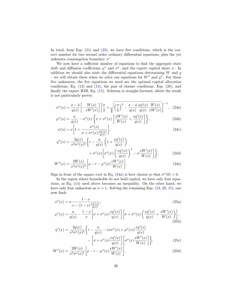
In total, from Eqs. (21) and (23), we have five conditions, which is the cor-rect number for two second order ordinary differential equations, plus the yetunknown consumption boundary x∗.

We now have a sufficient number of equations to find the aggregate statedrift and diffusion coefficients µx and σx, and the expert capital share ψ. Inaddition we should also state the differential equations determining W and q– we will obtain these when we solve our equations for W ′′ and q′′. For thesefive unknowns, the five equations we need are the optimal capital allocationconditions, Eq. (13) and (14), the pair of closure conditions, Eqs. (20), andfinally the expert HJB, Eq. (15). Solution is straight-forward, albeit the resultis not particularly pretty:

σx(x) =a− aq(x)

[− W (x)

xW ′(x)

][σ

2+

√(σ2

)2− a− a

q(x)

xq′(x)

q(x)

W (x)

xW ′(x)

]−1, (24a)

µx(x) =a

q(x)− σx(x)

σ + σx(x)

[xW ′(x)

W (x)+xq′(x)

q(x)

], (24b)

ψ(x) = x

[1 +

σx(x)

σ + σx(x)xq′(x)q(x)

], (24c)

q′′(x) =2q(x)

x2σx(x)2

r − a

q(x)

(1 +

xq′(x)

q(x)

)+ σx(x)

[σx(x)

(xq′(x)

q(x)

)2

− σxW′(x)

W (x)

], (24d)

W ′′(x) =2W (x)

x2σx(x)2

[ρ− r − µx(x)

xW ′(x)

W (x)

]. (24e)

Sign in front of the square root in Eq. (24a) is here chosen so that σx(0) > 0.In the region where households do not hold capital, we have only four equa-

tions, as Eq. (14) used above becomes an inequality. On the other hand, wehave only four unknowns as ψ = 1. Solving the remaining Eqs. (13, 20, 15), onenow finds

σx(x) = σ1− x

x− (1− x)xq′(x)q(x)

, (25a)

µx(x) =a

q(x)− 1− x

x

[σ + σx(x)

xq′(x)

q(x)

][σ + σx(x)

(xq′(x)

q(x)+xW ′(x)

W (x)

)],

(25b)

q′′(x) =2q(x)

x2σx(x)2

r − a

q(x)− (σσx(x) + µx(x))

xq′(x)

q(x)

−[σ + σx(x)

xq′(x)

q(x)

][σx(x)

xW ′(x)

W (x)

], (25c)

W ′′(x) =2W (x)

x2σx(x)2

[ρ− r − µx(x)

xW ′(x)

W (x)

]. (25d)

26

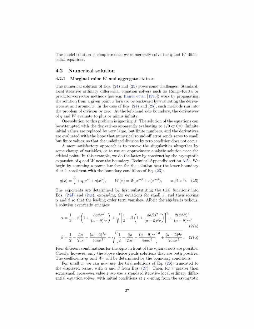
The model solution is complete once we numerically solve the q and W differ-ential equations.

4.2 Numerical solution4.2.1 Marginal value W and aggregate state x

The numerical solution of Eqs. (24) and (25) poses some challenges. Standard,local iterative ordinary differential equation solvers such as Runge-Kutta orpredictor-corrector methods (see e.g. Hairer et al. [1993]) work by propagatingthe solution from a given point x forward or backward by evaluating the deriva-tives at and around x. In the case of Eqs. (24) and (25), such methods run intothe problem of division by zero: At the left-hand side boundary, the derivativesof q and W evaluate to plus or minus infinity.

One solution to this problem is ignoring it: The solution of the equations canbe attempted with the derivatives apparently evaluating to 1/0 or 0/0. Infiniteinitial values are replaced by very large, but finite numbers, and the derivativesare evaluated with the hope that numerical round-off error sends zeros to smallbut finite values, so that the undefined division by zero condition does not occur.

A more satisfactory approach is to remove the singularities altogether bysome change of variables, or to use an approximate analytic solution near thecritical point. In this example, we do the latter by constructing the asymptoticexpansion of q and W near the boundary [Technical Appendix section A.5]. Webegin by assuming a power law form for the solution near the lower boundarythat is consistent with the boundary conditions of Eq. (23):

q(x) =a

r+ q1x

α + o(xα), W (x) = W1x−β + o(x−β), α, β > 0. (26)

The exponents are determined by first substituting the trial functions intoEqs. (24d) and (24e), expanding the equations for small x, and then solvingα and β so that the leading order term vanishes. Albeit the algebra is tedious,a solution eventually emerges:

α =1

2− β

(1 +

aaβσ2

(a− a)2r

)+

√[1

2− β

(1 +

aaβσ2

(a− a)2r

)]2+

2(aβσ)2

(a− a)2r,

(27a)

β =1

2− aρ

2ar− (a− a)2r

4aaσ2+

√[1

2− aρ

2ar− (a− a)2r

4aaσ2

]2+

(a− a)2r

2aaσ2. (27b)

Four different combinations for the signs in front of the square roots are possible.Clearly, however, only the above choice yields solutions that are both positive.The coefficients q1 and W1 will be determined by the boundary conditions.

For small x, we can now use the trial solutions of Eq. (26), truncated tothe displayed terms, with α and β from Eqs. (27). Then, for x greater thansome small cross-over value ε, we use a standard iterative local ordinary differ-ential equation solver, with initial conditions at ε coming from the asymptotic

27

0.0 0.1 0.2 0.3 0.4 0.5

1.4

1.5

1.6

1.7

1.8

1.9

2.0

x

qHxL

(a) Capital price q as a function of theaggregate expert net worth share x.

0.0 0.1 0.2 0.3 0.4 0.5

1.0

1.5

2.0

2.5

3.0

3.5

x

WHxL

(b) Marginal value of expert net worthas a function of the aggregate expert networth share x.

Figure 1: Numerical solution of Eqs. (24) and (25).

expansion. Value of ε should be large enough to ensure that evaluating thederivatives is not significantly affected by round-off error, but small enough sothat the asymptotic expansion is accurate. As a first guess, the square root ofthe maximum relative error of the used floating point arithmetic, ε ∼ 10−8 fordouble precision, can be used.

Using the above approach, we can now solve the q and W differential equa-tions given q1 and W1, the coefficients of the leading non-constant terms in theasymptotic expansion of q and W Eq. (26). We can arbitrarily fix W1 as theequations are invariant in linear scaling of W , and scale the solution ex-post inorder to satisfy the condition W (x∗) = 1 at the consumption boundary. Westill have q1 and the position of the upper boundary x∗ to be set so that theremaining boundary conditions W ′(x∗) = q′(x∗) = 0 are satisfied.

A simple numerical scheme that finds q1 and x∗ can be setup as follows:Define Θ(q1) as q′ evaluated at first x such that W ′(x) = 0 where q and W aresolutions to the model equations for the given q1. This point can be found bysolving the differential equations forward from the initial point, until the W ′(x)boundary is crossed; the exact crossing point is then polished using standardroot finding methods. The correct q1 can then be determined by finding Θ(q1) =0, where again, any standard root finding method can be employed.

In Fig. 1 we have plotted the numerical solution following the method de-scribed above. The parameter values used are a = 0.11, a = 0.07, σ = 0.1,r = 0.05, and ρ = 0.06.

28

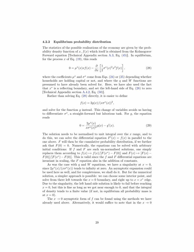
4.2.2 Equilibrium probability distribution

The statistics of the possible realisations of the economy are given by the prob-ability density function of x, f(x) which itself is obtained from the KolmogorovForward equation [Technical Appendix section A.3, Eq. (45)]. In equilibrium,for the process x of Eq. (19), this reads

0 = µx(x)xf(x)− ∂

∂x

[1

2σx(x)2x2f(x)

], (28)

where the coefficients µx and σx come from Eqs. (24) or (25) depending whetherhouseholds are holding capital or not, and where the q and W functions arepresumed to have already been solved for. Here, we have also used the factthat x∗ is a reflecting boundary, and set the left-hand side of Eq. (28) to zero[Technical Appendix section A.4.2, Eq. (50)].

Rather than solving Eq. (28) directly, it is easier to define

f(x) = 2g(x)/(xσx(x))2,

and solve for the function g instead. This change of variables avoids us havingto differentiate σx, a straight-forward but laborious task. For g, the equationreads

0 =2µx(x)

xσx(x)2g(x)− g′(x). (29)

The solution needs to be normalised to unit integral over the x range, and todo this, we can solve the differential equation F ′(x) = f(x) in parallel to theone above. F will then be the cumulative probability distribution, if we furtherask that F (0) = 0. Numerically, the equations can be solved with arbitraryinitial conditions: If f and F are such un-normalised solutions, one simplyreplaces them according to f(x) 7→ f(x)/[F (x∗) − F (0)] and F (x) 7→ [F (x) −F (0)]/[F (x∗)− F (0)]. This is valid since the f and F differential equations areinvariant in scaling, the F equation also in the addition of constants.

As was the case with q and W equations, we have a singularity at x = 0,since 2µx(x)/(xσx(x)) tends to infinity at zero. An asymptotic expansion couldbe used here as well, and for completeness, we shall do it. But for the numericalsolution, a simpler approach is possible: we can choose some interior point, andsolve from there left towards the x = 0 boundary, and right up to x = x∗ edge.Due to the singularity, the left hand side solution is likely to fail before reachingx = 0, but this is fine as long as we got near enough to 0, and that the integralof density tends to a finite value (if not, in equilibrium all probability mass isat x = 0).

The x → 0 asymptotic form of f can be found using the methods we havealready used above. Alternatively, it would suffice to note that in the x → 0

29

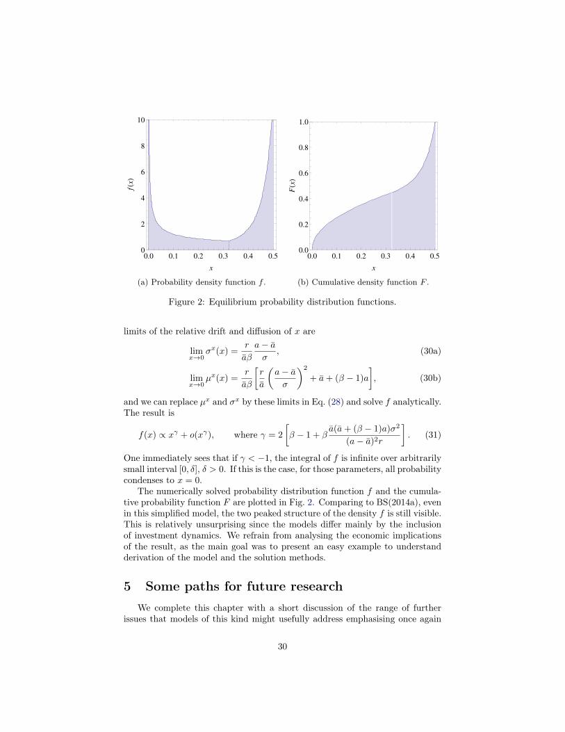
0.0 0.1 0.2 0.3 0.4 0.50

2

4

6

8

10

x

fHxL

(a) Probability density function f .

0.0 0.1 0.2 0.3 0.4 0.50.0

0.2

0.4

0.6

0.8

1.0

x

FHxL

(b) Cumulative density function F .

Figure 2: Equilibrium probability distribution functions.

limits of the relative drift and diffusion of x are

limx→0

σx(x) =r

aβ

a− aσ

, (30a)

limx→0

µx(x) =r

aβ

[r

a

(a− aσ

)2

+ a+ (β − 1)a

], (30b)

and we can replace µx and σx by these limits in Eq. (28) and solve f analytically.The result is

f(x) ∝ xγ + o(xγ), where γ = 2

[β − 1 + β

a(a+ (β − 1)a)σ2

(a− a)2r

]. (31)

One immediately sees that if γ < −1, the integral of f is infinite over arbitrarilysmall interval [0, δ], δ > 0. If this is the case, for those parameters, all probabilitycondenses to x = 0.

The numerically solved probability distribution function f and the cumula-tive probability function F are plotted in Fig. 2. Comparing to BS(2014a), evenin this simplified model, the two peaked structure of the density f is still visible.This is relatively unsurprising since the models differ mainly by the inclusionof investment dynamics. We refrain from analysing the economic implicationsof the result, as the main goal was to present an easy example to understandderivation of the model and the solution methods.

5 Some paths for future researchWe complete this chapter with a short discussion of the range of further

issues that models of this kind might usefully address emphasising once again

30

that this is still an immature literature, that many technical challenges remainand therefore we can make no firm predictions about where contributions andbreakthroughs will come.

There are many paths of future investigation that could be followed. Anumber of contributions to the new continuous-time macrofinancial literatureassume an ‘AK’ production function i.e. output is a linear function of the stockof capital. This assumption, which can be traced back to the contribution ofFrankel [1962], was widely employed in the earlier contributions to the literatureon endogenous growth (see Aghion and Howitt [2009] for review of this litera-ture). Both Isohätälä et al. [2014b] and Brunnermeier and Sannikov [2014b] canbe interpreted as models of endogenous growth yielding the prediction that capi-tal accumulation and hence the rate of economic growth will fall when corporatenet worth falls and that the economy may then remain for an extended period ina phase of low investment and low growth (the ‘net worth’ trap). These modelsmay thus already provide some insight into the major puzzle of the slowdownof aggregate productivity growth in many countries since the global financialcrisis.

This is though a rather simplistic account of growth. The theoretical growthliterature has moved on to focus on other mechanisms such as investment inproduct variety (as in Romer [1987, 1990]) and in the discovery of new moreefficient methods of production (innovation) that replace older inferior methods(e.g. the model of Schumpterian ‘creative destruction’ of Aghion and Howitt[1992]). A natural further development will therefore be to employ similar con-tinuous time models to examine the impact of balance sheet constraints andfinancial distress on investment in new products and processes and hence onproductivity growth. Doing this though may be difficult within the currentassumption of only a single state variable.

A related issue is that of structural adjustment following financial crises.Many countries need to adjust the structure of their economies, for exampleswitching labour and capital resources from non-traded to traded output. Ris-ing risk-premia in periods of financial distress can act as a barrier to such in-vestments, providing another form of trap in a low-output low-income state.Other similar issues arise in understanding the low elasticities of traded sectoroutput to changes in exchange rates following financial crises or in the responseof small open economies to ‘sudden stops’ of capital flows (on this issue Brun-nermeier and Sannikov [2014a] have made a promising start using continuoustime methods).

Further understanding will surely also need to take account of the interactionof balance sheet constraints with household, corporate and bank expectationsabout future productivity and incomes. To date the continuous-time macrofi-nancial literature has imposed the conventional but rather strong assumption ofmodel-consistent expectations. Every agent is assumed to know both the currentstate of the economy and stochastic processes that drives both the state of theeconomy and market prices. Different, possibly even more extended, dynamicscan be expected when agents update their expectations about unobserved statesand processes in response to their current observations. Thus, for example, a

31

fully adequate model of endogenously created bank inside-money would seem toneed to take account of the possibility that optimistic expectations about futureincome result in a period of rapid and self-reinforcing expansion of both bankcredit and bank money. Introducing learning of this kind into these models willbe a further technical challenge.

A further potential line of inquiry is to make the treatment of financialmarkets more realistic, for example by allowing for alternative (financial mar-kets) source of financing for the productive sector, on top of bank loans, sincethe empirical evidence suggests that firms tend to partly substitute bank fi-nancing by market financing when credit conditions tighten (see e.g., Beckerand Ivashina [2014]). This would help to get a better understanding of howthe substitutability of funding sources can add to/mitigate the propagation offundamental shocks, with the implications for growth and financial stability.Another similar departure would be to allow for the internal source of financingfor the productive sector (i.e., capital accumulation within firms). Introducingthis feature, most likely, would require introducing an additional state variablein play – the net worth of the productive sector, which might be technicallychallenging.29

Similarly there is need for better understanding of the role of both commer-cial and central bank balance sheets in macroeconomic transmission and thesupply of credit. The DSGE assumption that all that matters in monetary pol-icy is interest rates is now accepted as an oversimplification, but we are not yetin the position of having tractable incomplete market models, in either contin-uous or discrete time, in which the role of commercial and central bank balancesheets is clearly articulated. While the work of Brunnermeier and Sannikov[2014e] that we have reviewed offers a particularly promising start, it is still notyet possible to say that the present ‘state of the art’ is sufficiently developed toprovide a full understanding of the impact of unorthodox monetary policy (cen-tral bank balance sheet expansion) or macroprudential tools (such as cyclicallyvarying capital requirements or limits on loan-to value ratios).

These paths for future research are far from exhausting the list of possi-ble applications of new continuous-time macrofinancial modelling. There arealso opportunities to apply this framework in a number of other settings moreroutinely explored using standard linearised DSGE models. Examples includemodelling the labour market, real wages and employment and product marketsand price setting. If balance sheet constraints affect investment and asset mar-kets then they should also affect labour and goods markets. Writing down suchmodels in continuous-time with balance sheet and net worth constraints doesnot seem so difficult. Solution though could be challenging because of the needto include additional state variables.

The challenges of numerical solution should give pause for thinking care-fully about the choice of modelling strategy. There are well developed toolsfor numerical solution of macroeconomic models with several state variables in

29In a discrete time set-up an attempt to accommodate this feature is made by Rampiniand Viswanathan [2012].

32

discrete time. Replicating all this technical work on solution with many statevariables in continuous-time may not be an efficient way to proceed. It mayinstead be more useful to find ways to incorporate the insights of continuous-time macrofinancial modelling into more widely known and understood discretetime settings. This is one reason why, as we have already suggested, we believethat over time the ‘gap’ between continuous-time and discrete time specifica-tions can and should be closed. There is no reason why the impact of balancesheet constraints and net worth cannot be incorporated into otherwise standarddiscrete-time specifications (although this may come at some cost, for examplethe need to introduce more explicit modelling of what happens when distur-bances result in constraints binding, something that can often be convenientlyput to one side when uncertainty is modelled as a continuous time diffusion).

Finally, of course, it will be essential to take these models closer to data.Some initial steps in this direction are already made by He and Krishnamurthy[2013, 2014] who seek to replicate the asset market behaviour during the 2007-2009 financial crisis. Improving predictive and simulation properties of thesemodels, however, carries a risk of losing tractability and transparency. Anillustration is the challenge of explaining the counterfactual prediction of Heand Krishnamurthy [2012] and He and Krishnamurthy [2013] that the leverageof financial intermediaries increases substantially during financial crises (theunderlying mechanism is that the emergence of crisis results from low specialistequity requiring them to leverage in order to maintain ‘skin in the game’).

As an example of the challenges of bring these models to the data, we canbriefly describe how the model by Adrian and Boyarchenko [2013] employscontinuous-time macro-financial modelling tools to develop an explanation ofobserved pro-cyclical intermediary leverage. There are several distinctive fea-tures of this work. Three of these seem to be particularly important. Firstthat financial intermediaries do not maximise an objective function (such aspresent discounted future dividends); instead, they behave mechanically, firstusing earnings to pay floating rate coupons on long term bonds issued to house-holds (the coupon rate is determined by equilibrium of the supply and demandfor these bonds) and retaining all remaining earnings to build up equity andinvest in productive capital. Second that if intermediary equity falls belowa lower boundary, then financial intermediaries are restructured, with debt-holders wiped out and re-established under new equity holders. Since all inter-mediaries are identical and hit by the same shocks this is a systemic crisis. Thirdthat financial intermediary leverage, and hence their investment in productivecapital, is continuously determined by a regulatory driven value at risk typeconstraint that depends on the short term volatility of the price of productivecapital.

Similar to the other macrofinancial models that we have described, all vari-able of interests (intermediary equity, the price of productive capital, the ex-pected excess returns on holding intermediaries’ debt and productive capital)can be described as the functions of a single state variable. Just as in He andKrishnamurthy [2012] and Brunnermeier and Sannikov [2014b] this state vari-able is the share of financial intermediaries’ net worth in total wealth. The

33

novel contribution are two closely related empirical predictions not captured byother models. First, as a direct consequence of the assumed leverage constraint,it generates the empirically-observed procyclical pattern of intermediary lever-age. Second it also explains what Adrian and Boyarchenko [2013] describe asthe volatility paradox, i.e. the well known observation that systemic risks tendto increase during periods of perceived low volatility e.g. for example duringthe ‘great moderation’ that preceded the global financial crisis. In their modelthis appears as a negative relationship between the instantaneous endogenousvolatility of the returns to holding capital with the probability of a systemicdefault. As endogenous volatility declines, leverage rises and thus also does therisk of a systemic default on a six-month ahead horizon (see their Figure 5.)

While Adrian and Boyarchenko [2013] make a valuable further contribution,their work can also be read as an illustration of the very substantial challengesof bringing models of this kind to the data. Departures from forward lookingbehaviour or inter-temporal optimisation are not necessarily wrong, but thesedepartures open up such a large menu of possible modelling choices that isdifficult to know what is the best way forward. There is an almost unlimitedrange of possible underlying assumptions of this kind that can generate macro-financial interactions.

In order to impose the required intellectual discipline, it may prove neces-sary to focus on developing models of incomplete markets that are consistent notjust with observed aggregate outcomes such as asset prices or national account-ing measures of output and investment (there are simply too many potentialmodelling choices for doing this), but also with micro-level data at the level ofindividual firms, households and financial institutions. In this context it willbe difficult to ignore the simplifying aggregation assumptions employed in thecontinuous-time macrofinancial literature. Instead it may eventually prove nec-essary to work with large scale agent-based models, in which distribution ofnet worth and leverage within sectors is tracked as well as the aggregate networth (see Haldane [2015] for further discussion of why macrofinancial mod-elling should use agent-based modelling). Work of this kind will though needa different approach to research than has been conventionally used in macroe-conomics, requiring relatively large teams of researchers in order to collect andmatch the underlying microlevel data.

6 ConclusionThis chapter has reviewed several contributions to a new and promising currentliterature, employing continuous time models to capture some of the macrofi-nancial interactions that have been highlighted by the global financial crisis.Though using highly stylized specifications, these models demonstrate how theinteraction of market incompleteness with the balance sheet constraints of eco-nomic agents can generate dynamics of macroeconomic variables much moreconsistent with the empirically observed patterns at times of crisis than thosegenerated by conventional DSGE models. These dynamics include substantial

34

variations in risk-premia and asset prices, as well as subsequent substantial andhighly persistent declines of macroeconomic aggregates such as output and in-vestment. In the models reviewed in this chapter these dynamics are largelydriven by what are in effect changes in attitudes to risk, and by externalitiesstemming from the fact that individual agents do not internalize the impact oftheir individual risk taking or other decisions on the wider economy.

As we highlight in Section 5 of this chapter, the modelling approach intro-duced by this new literature has the potential to address a large spectrum ofmacroeconomic problems. The pursuit of these avenues of future research isan exciting challenges, from both technical and economic perspectives. Wherethen will future research ultimately take us? We have no crystal ball but ourjudgment is that the eventual destination of this literature will be a relativelysmall number of comparatively simple but influential continuous-time modelsof the kind we review here, providing widely accepted economic intuition andpolicy insight into macrofinancial interactions rather than predicting accuratelymacroeconomic and financial market developments.

An important impact of these modelling efforts may be persuading researchersworking in more conventional discrete-time frameworks of the necessity of tak-ing incomplete markets and balance sheet and net worth constraints seriously.Matching with data is then in turn likely to require more ‘agent-based’ ap-proaches in order to meet the fundamental challenge of aggregation.

Such research will need a very careful process of matching against bothmicrolevel and aggregate data in order to develop useful models. The finaloutcome could be a shift in modelling paradigms, from the typical small teamwork found in much current macro-economics to more resource intensive in-vestigations involving many investigators and massive efforts at data-collectionand calibration, with the overall direction of research guided to an importantdegree by the insights of the new continuous-time approach to macrofinancialmodelling.

This does not avoid the need for considerable efforts in order to find a rea-sonable balance between on the one hand transparency and clear economic in-tuition, and on the other the realism and accuracy of underlying economic as-sumptions. We believe that the new macrofinancal modelling, despite the use oftechniques of continuous-time stochastic modelling with which most economistsare not very familiar, are especially useful because of the relatively clear andsimple intuitions they provide about the macroeconomic consequences of incom-plete markets and hence the resulting impact of balance sheet and net worthon macroeconomic outcomes. We therefore hope this chapter can be helpful inacquainting our readers with the conceptual and technical features of this newgeneration of models and stimulating interest in this field of research.

A Appendix: Basics of continuous time modelsIn this appendix, we review some technical issues that arise when trying tounderstand, construct, or solve models that incorporate binding financing con-

35

straints in continuous time models. We begin with a brief summary of key con-cepts, eschewing formal proofs and favouring heuristic derivations that nonethe-less can in principle be used as a basis for more rigorous approach.

A.1 Stochastic differential equationsThe primary modeling tool for describing the state of an agent is the stochasticdifferential equation (SDE), a generalisation of the ordinary differential equationthat incorporates some form of external stochastic forcing. Gardiner [2009]gives an excellent and approachable review of many of the topics covered hereand subsequent sections; other solid reference texts on stochastic differentialequations include Ø ksendal [2003] and Feller [1971].

Let xt stand for an agent’s state, e.g. wealth or net worth, at time t, withthe initial, t = 0 state x0 given. We say x is a diffusion process and formallywrite its equation of motion as the SDE

dxt = µ(xt) dt+ σ(xt) dzt, (32)

where zt is aWiener process, a continuous stochastic process having independentand normally distributed increments, zt+h−zt =

√hη, where η is a unit normal

distributed random variable. The differentials, dxt,dzt, . . ., can be viewed asthe zero time step limits of corresponding finite differences, so that Eq. (32)becomes the limit of the discrete time model

x(k+1)T = xkT + Tµ(xkT ) +√Tσ(xkT )ηkT , (33)

where T , T → 0, is the length of the period and ηkT , k = 0, 1, . . ., are in-dependent unit normal distributed random variables30. More rigorously, thestochastic differential equation, Eq. (32) should be understood as a short-handway of writing the stochastic integral

xt = x0 +

ˆ t

0

µ(xs)ds+

ˆ t

0

σ(xs)dzs, (34)

where the integral against the Wiener process, or any diffusion process in gen-eral, is defined analogously to the Riemann-Stieltjes integral. Stochastic calculusis the theory of stochastic differential equations; for a more focused reference onthe topic, we refer the reader to e.g. Klebaner [2005].

An important analytical tool is the Itô’s Lemma which allows one to differ-entiate functions of diffusion processes such as x as given by Eq. (32). If f is

30The above uses the Itô interpretation of the SDE (32) which amounts to assuming that thenoise amplitude σ is evaluated at the start of each period. In general one can set x(k+1)T =

xkT + Tµ(xkT ) +√Tσ(xkT+α)ηkT where 0 ≤ α ≤ 1. Choice of α does influence the form of

later formulas. The Itô interpretation, α = 0 is the default choice in economics applications,as equations of motion are supposed not to pre-empt the shocks. In natural sciences, theStratonovich convention α = 1/2 is commonly used.

36

any twice differentiable function defined in the domain of x, then f evaluatedat xt, denoted ft = f(xt), is also a diffusion process with the increments

dft =

[∂f(xt)

∂t+ µ(xt)

∂f(xt)

∂x+

1

2σ(xt)

2 ∂2f(xt)

∂x2

]dt+

∂f(xt)

∂xσ(xt) dzt. (35)

Although we focus on single state variable problems, equivalent equationsfor multivariate case are still useful. For instance, in the construction of ourexample model, we needed multivariable formulas as we reduced an initiallytwo variable problem to a single variable. Suppose Xt is an N -dimensionaldiffusion process taking values on some subset of RN , Xt = (x1t , x

2t , . . . , x

Nt )T

(here T stands for matrix transposition). We write the X equation of motion as

dXt = µ(Xt) dt+ σ(Xt) dZt, (36)

where now Z is a vector of Wiener processes, Zt = (z1t , . . . , zKt )T, K is the

number of independent shock sources, µ(Xt) = (µ1(Xt), . . . , µN (Xt))

T is thedrift vector and σ(Xt) = [σij(Xt)]ij is the N × K covariance matrix. Theelements of Zt can be without loss of generality taken to be independent: anyand all instantaneous correlations between shocks are encoded in the matrix σ.

The multivariate version of Itô’s Lemma, Eq. (35), for a function f = f(X),f : RN 7→ R, reads

dft =

µ(Xt)

T∇Xf(Xt) +1

2tr[σ(Xt)

THXf(Xt)σ(Xt)]

dt

+∇Xf(Xt)Tσ(Xt) dZt, (37)

where tr stands for matrix trace, and ∇Xf and HXf give the gradient vectorand the N × N Hessian matrix of the function f , [∇Xf(X)]i = ∂f(X)/∂xi,[HXf(X)]ij = ∂2f(X)/∂xi∂xj .

These equations assume that the SDEs do not depend explicitly on timet, that is, they are time-homogeneous. An easy way of extending all of thesedefinitions to account for explicit time dependence is to consider t additionalstate variable in X, with the trivial SDE dt = dt.

A.2 Hamilton-Jacobi-Bellman equationThe standard tool in stochastic dynamical programming is the Hamilton-Jacobi-Bellman equation [Fleming and Soner, 2006]. Suppose that equations of motion,Eqs. (32) and (36) in the multivariate case depend on some controls y, whichwe now wish to choose so that our discounted future utility is maximal. Foran infinite time-horizon problem, with standard exponential discounting andtime-preference rate ρ, the objective function to maximise is

Ω(x0; yt∞t=0) = Eˆ ∞0

e−ρtu(yt) dt, (38)

37

where u is the utility function. Let V then be the maximal Ω, and henceforthassume that y refers to the maximiser:

V (x) = maxyt∞t=0

Ω(x0; yt∞t=0). (39)

Assuming that V is twice differentiable, it can be found as a solution to theHamilton-Jacobi-Bellman (HJB) equation:

ρV (x) = maxy

u(y) + µ(x, y)V ′(x) +

1

2σ(x, y)2V ′′(x)

. (40)

An easy heuristic derivation goes as follows: (i) Start with the definition ofV and divide the integral into two parts: from 0 to some small h, and fromh to infinity; (ii) Use Bellman’s principle on the second integral to make itV a time h later, appropriately discounted, e−ρhV (xh); (iii) Use Itô’s Lemmato approximate V (xh), Taylor expand in h, and then let h → 0. This basicderivation of the Hamilton-Jacobi-Bellman equation requires that V be twicedifferentiable. It is well known that solutions do not always have this property.The theory of viscosity solutions addresses this problem, however, this topic isbeyond the scope of this introduction (See e.g. Fleming and Soner [2006], orCrandall et al. [1992] for a rigorous but self-contained guide to the subject).

Generalising to the multivariate case, the Hamilton-Jacobi-Bellman equationfor the process of Eq. (36) with controls y reads:

ρV (X) = maxy

u(y) + µ(X)T∇XV (X) +

1

2tr[σ(X)THXV (X)σ(X)

]. (41)

A.3 Equilibrium characterisationIn the conventional view, persistent e.g. in much of DSGE modeling today,what constitutes an equilibrium is a point in state space, plus random fluctua-tions induced by shocks. Such equilibria are a feature of, say, models linearisedaround a deterministic steady state, and which treat shocks as relatively smallperturbations. When the modeling paradigm allows for large deviations, as isthe case in the models we are highlighting here, this point-plus-perturbationspicture of the equilibrium breaks down. Shocks, possibly amplified by feedbackeffects, can now drive the system far from what would have traditionally beenseen as a relatively tranquil equilibrium point. Rather then, the equilibrium ischaracterised by a probability distribution over the whole state space.

In continuous time, the probability distribution of a diffusion process x isgiven by the Kolmogorov forward equation, also known as the Fokker-Planckequation (See e.g. Gardiner [2009]; Risken [1996] is solely dedicated this equa-tion): If f(t, x|x0) is the probability density function of process x followingEq. (32) with initial data x0, then f satisfies the partial differential equation(omitting the explicit conditioning on the initial x):

∂f

∂t(t, x) = − ∂

∂x

µ(x)f(t, x)− ∂

∂x

[1

2σ(x)2f(t, x)

]. (42)

38

Probability densities are integrated to get actual probabilities: Given a largenumber of independent realisations of x, the probability of finding x in theinterval [x0, x1] at time t is

Pt(xt ∈ [x, x+ ∆x]) =

ˆ x1

x0

f(t, x′) dx′. (43)

The “large number of independent realisations” can be understood either asmany simultaneously running independent processes (and so with independentshocks), or as a large number of samples of a single process, taken over an in-finitely long time period. In the former view, f(x) represents the cross-sectionaldensity of the state variables following the same dynamic stochastic equationsof motion. Which view is correct depends of course on what one aims to model.

For additional intuition, the forward equation can be written in the form ofa continuity equation relating the temporal change of f to spatial variation ofa probability flux:

∂f

∂t(t, x) = − ∂j

∂x(t, x), (44a)

j(t, x) = µ(x)f(t, x)− ∂

∂x

[1

2σ(x)2f(t, x)

], (44b)

where j(t, x) is the probability current, that is, the rate of flow of probabilitythrough the point x to the positive x direction. In equilibrium ∂f(t, x)/∂t =0, and therefore the Fokker-Planck equation reduces to a first order ordinarydifferential equation

µ(x)f(t, x)− ∂

∂x

[1

2σ(x)2f(t, x)

]= j0, (45)

where j0 is a constant to be determined by the boundary conditions.The multivariate Fokker-Planck equation corresponding to the process X,

again taking values on RN and following the SDE (36), is in turn

∂f

∂t(t,X) = −∇X · J(t,X) (46a)

J(t,X) = µ(X)f(t,X)−∇X ·[

1

2σ(x)Tσ(x)f(t,X)

], (46b)

where J = (j1, . . . , jN )T is now an N -dimensional probability current, and ∇X ·is the divergence operator, ∇X ·J(X) =

∑Ni=1 ∂j

i(X)/∂xi, [∇X ·σ(x)Tσ(X)]i =∑Nj=1 ∂[σ(x)Tσ(x)]ij/∂x

j .

A.4 Boundary conditionsSolutions to the HJB and the Fokker-Planck equations, Eqs. (40) and (44), orEqs. (41) and (46) in the multivariate case, are not uniquely fixed until appro-priate boundary conditions are given. Nonlinearity, capital constraints, and the

39

need for proper treatment boundary conditions go hand in hand: If one is toconstruct a model that can account for large fluctuations, one must account forthe possibility of a state variable hitting a hard bound, e.g. a capital or leverageconstraint. Here, we consider the two most common boundary conditions: theabsorbing and (instantaneously) reflecting boundary.

A.4.1 Absorbing boundary

An absorbing boundary, say placed at position x†, is such that upon reachingit, the process is stopped and removed from the distribution. A stopped process(an agent who goes out of business, or a firm that has been liquidated) canno longer generate utility, and so it is natural to require that at an absorbingboundary value is zero,

V (x†) = 0, (47)

whenever of course the utility function is non-negative for all controls. For theprobability density, an absorbing boundary at x† means that

f(x†) = 0, (48)

which has the natural interpretation of asking that point x† is always completelyfree of the process x.

Multivariate generalisations are obvious: The absorbing boundary is not apoint anymore, but some surface in the embedding space, and the same zerovalue or zero density requirement holds.

A.4.2 Reflecting boundary

Although the word reflection invokes a picture of a very certain type of motion,such as elastic bouncing of a ball off of a rigid wall, or specular reflection ofa beam of light, a reflecting boundary is here understood somewhat more gen-erally: We will call a boundary reflecting whenever it conserves probabilitiesin the sense that it does not leak probability in or out, or allow the processaccumulate or stop there for a finite time period.

In general, a reflecting boundary is setup by some forcing term that is strongenough to overcome the drift and diffusion terms in Eq. (32), preventing the pro-cess from ever crossing the boundary. Such forcing can be due to e.g. a singularcontrol term (a control that has unbounded magnitude and which optimallyis always either fully on or off). A rigorous mathematical treatment of SDEswith reflection does not use infinitely strong drift terms31, but as a model toguide intuition, the idea that the boundary is enforced by infinitely strong andinfinitely short kicks is reasonable enough.

31A standard approach is recasting the SDE with reflection into a so called Skorokhodproblem, whereby the process x is seen as driven by an additional process k, dxt = µ(xt) dt+σ(xt) dzt+dkt, and where dkt is non-zero only on the boundary. See e.g. Lions and Sznitman[1984].

40

For functions of process x, a reflecting boundary implies a Neumann condi-tion: it imposes a specific value on the derivative of the function. Say there isa reflecting boundary at x∗. For the value function, we then must have that

V ′(x∗) = 0. (49)

This can be justified as follows: imagine the x range inside the boundary re-flected into the range outside the boundary. One can now view a process hittingthe boundary as instead passing into the “mirror” space. In order for V to besmooth across the boundary, demanded by the smoothness of optimal V , thenthe derivative V ′ is zero. Similarly, for any continuously differentiable functionof the process, the derivative should vanish at x∗.

For the density f , a reflecting boundary naturally corresponds to a pointwhere the probability current j, Eq. (44), vanishes

j(x∗) = µ(x)f(x)− ∂

∂x

1

2σ(x)2f(x)

∣∣∣∣x=x∗

= j0 = 0. (50)

Note that in the one-dimensional case, in steady state, this condition fixes theprobability flow to zero over the whole of the x range. If there is also a reachableabsorbing state, the probability density must be over the x range, for then boththe value and derivative of f vanish at the same time. The word reachable iskey: An absorbing boundary may be such that it cannot be arrived at in finitetime. In this case, both an absorbing and reflecting boundary can co-exist, withthe probability density not collapsing to zero.

Extensions to N -dimensional processes X are somewhat more complicatedthan for the absorbing boundary. Suppose that the reflecting boundary is asurface in RN , x∗ is a point on that surface, and that Γ(x∗) is the direction ofthe boundary forcing term (assumed never perpendicular to the normal of theboundary). Then the boundary condition for V reads

Γ(x∗) · ∇XV (x∗) = 0, (51)

that is, the Γ-directed derivative of V is zero when on an reflecting boundary.For the Fokker-Planck equation, the N -variable extension Eq. (50) is

ν(x∗) · J(x∗) = 0, (52)

where ν(x∗) is the inwards unit normal vector of the boundary surface at x∗, andJ is the probability current as given by Eq. (46b). The natural interpretationis that the probability flow perpendicular to the surface is zero (no outflow ofprobability, or accumulation on the surface).

A.5 Asymptotic analysisA useful tool in studying the behaviour of continuous time models is the asymp-totic expansion. These are simply approximate analytical solutions of the modelequations that are valid only near the boundaries. Their utility lies in the fact

41

that they can yield analytic insight into the qualitative and quantitative be-haviour of the model near the boundaries, which in turn can aid the modelanalysis or help with the numerical solution of the equations.

The exact way of constructing the expansion varies from problem to problem,but the general idea is to use the smallness of the distance to the boundary, orthe greatness of the variable if very far from it, as a simplifying assumption. Afairly generally applicable recipe goes as follows:

1. Guess the limiting form of the solution, oftentimes a power law of theindependent variable.

2. Substitute this trial function into the equation to be solved.

3. Expand the equation to leading order by neglecting terms that are guar-anteed to be smaller than other terms in the equation.

4. Choose the parameters of the trial function so that a solution matchingthe boundary constraints are satisfied.

B References

Tobias Adrian and Nina Boyarchenko. Interdiary Leverage Cycles and Finan-cial Stability. 2013. URL http://www.newyorkfed.org/research/staff_reports/sr567.pdf.

Philippe Aghion and Peter Howitt. A Model of Growth Through Creative De-struction. Econometrica, 60(2):323–351, March 1992. ISSN 00129682. doi:10.2307/2951599. URL http://www.jstor.org/stable/2951599.

Philippe Aghion and Peter Howitt. THE ECONOMICS OF GROWTH. MITPress, Boston, 2009.

S Rao Aiyagari. Uninsured idiosyncratic risk and aggregate saving. The Quar-terly Journal of Economics, 109(3):659–684, 1994. ISSN 0033-5533.

Yann Algan, Olivier Allais, Wouter J Den Haan, and Pontus Rendahl. Solvingand simulating models with heterogeneous agents and aggregate uncertainty.Handbook of Computational Economics, 2010.

Bo Becker and Victoria Ivashina. Cyclicality of credit supply: Firm levelevidence. Journal of Monetary Economics, 62:76–93, March 2014. ISSN03043932. doi: 10.1016/j.jmoneco.2013.10.002.

42

Ben Bernanke, Mark Gertler, and Simon Gilchrist. The Financial Acceleratorin a Quantitative Business Cycle Framework. In John B Taylor and MichaelWoodford, editors, Handbook of Macroeconomics, Volume 1C, pages 1341–1393. Elsevier Science, North-Holland, 1999.

Fischer Black and Myron Scholes. The pricing of options and corporate liabili-ties. The journal of political economy, pages 637–654, 1973. ISSN 0022-3808.

Patrick Bolton, Hui Chen, and Neng Wang. A Unified Theory of Tobin’sq, Corporate Investment, Financing, and Risk Management. The Jour-nal of Finance, 66(5):1545–1578, October 2011. ISSN 00221082. doi:10.1111/j.1540-6261.2011.01681.x. URL http://doi.wiley.com/10.1111/j.1540-6261.2011.01681.x.

Markus K Brunnermeier and Yuliy Sannikov. Macro, Money and Finance: AContinuous-Time Approach. In John Taylor and Harald Uhlig, editors, Hand-book of Macroeconomics Vol 2.

Markus K. Brunnermeier and Yuliy Sannikov. International Credit Flows, Pe-cuniary Externalities, and Capital Controls. 2014a.

Markus K. Brunnermeier and Yuliy Sannikov. A Macroeconomic Modelwith a Financial Sector. American Economic Review, 104(2):379–421, February 2014b. ISSN 0002-8282. doi: 10.1257/aer.104.2.379. URL http://www.ingentaconnect.com/content/aea/aer/2014/00000104/00000002/art00002.

Markus K Brunnermeier and Yuliy Sannikov. A Macroeconomic Modelwith a Financial Sector: online appendix. American Economic Re-view, (2), February 2014c. ISSN 0002-8282. doi: 10.1257/aer.104.2.379. URL http://www.ingentaconnect.com/content/aea/aer/2014/00000104/00000002/art00002.

Markus K Brunnermeier and Yuliy Sannikov. The I Theory of Money: versionof April 2014. 2014d.

Markus K Brunnermeier and Yuliy Sannikov. The I Theory of Money: versionof November 2014. 2014e.

Markus K Brunnermeier, Thomas M Eisenbach, and Yuliy Sannikov. Macroe-conomics with financial frictions: A survey. Technical report, 2012.

Guillermo A. Calvo. Capital Market Crises. Journal of Applied Economics, 1(1):35–54, 1998.

George M Constantinides. Intertemporal asset pricing with heterogeneous con-sumers and without demand aggregation. Journal of Business, pages 253–267,1982. ISSN 0021-9398.

43

Michael G Crandall, Ishii Hitoshi, and P.-L. Lions. User’s guide to viscositysolutions of second order partial differential equations. Bull. Amer. Math.Soc., 27:1–67, 1992.

Harry DeAngelo and René M Stulz. Why high leverage is optimal for banks.Technical report, 2013.

Wouter J. Den Haan. Comparison of solutions to the incomplete mar-kets model with aggregate uncertainty. Journal of Economic Dynam-ics and Control, 34(1):4–27, January 2010. ISSN 01651889. doi: 10.1016/j.jedc.2008.12.010. URL http://www.sciencedirect.com/science/article/pii/S0165188909001298.

Douglas Diamond and Phillip Dybvig. Bank runs, deposit insurance and liquid-ity. Journal of Political Economy, 91:401–419, 1983.

Douglas W. Diamond. Financial Intermediation and Delegated Monitoring.The Review of Economic Studies, 51(3):393, July 1984. ISSN 00346527. doi:10.2307/2297430. URL http://restud.oxfordjournals.org/content/51/3/393.short.

William Feller. An Introduction to Probability Theory and its Applications,volume II. Wiley, New York, 2nd edition, 1971.

ZHIGANG FENG, JIANJUN MIAO, ADRIAN PERALTA-ALVA, andMANUEL S SANTOS. NUMERICAL SIMULATION OF NONOPTIMALDYNAMIC EQUILIBRIUM MODELS. International Economic Review, 55(1):83–110, February 2014. ISSN 1468-2354. doi: 10.1111/iere.12042. URLhttp://dx.doi.org/10.1111/iere.12042.

Wendell Fleming and Halil Mete Soner. Controlled Markov Processes andViscosity Solutions. Stochastic Modelling and Applied Probability. Springer,New York, 2nd edition, 2006.

Marvin Frankel. The production function in allocation and growth: a synthesis.The American Economic Review, pages 996–1022, 1962. ISSN 0002-8282.

Crispin Gardiner. Stochastic Methods: A Handbook for the Natural and SocialSciences. Springer Series in Synergetics. Springer, Berlin, 4th edition, 2009.

William M Gorman. Separable utility and aggregation. Econometrica: Journalof the Econometric Society, pages 469–481, 1959. ISSN 0012-9682.

Luca Guerrieri and Matteo Iacoviello. OccBin: A toolkit for solving dy-namic models with occasionally binding constraints easily. Journal of Mon-etary Economics, 70:22–38, March 2015. ISSN 03043932. doi: 10.1016/j.jmoneco.2014.08.005. URL http://www.sciencedirect.com/science/article/pii/S0304393214001238.

44

Fatih Guvenen. Macroeconomics with hetereogeneity: a practical guide. Eco-nomic Quarterly, (3Q):255–326, 2011.

Ernst Hairer, Gerhard Wanner, and Syvert P Nø rsett. Solving Ordinary Dif-ferential Equations I: Nonstiff Problems. Springer Series in ComputationalMathematics. Springer, Berlin, 1993.

Andrew G Haldane. On microscopes and telescopes, 2015. URLhttp://www.bankofengland.co.uk/publications/Documents/speeches/2015/speech812.pdf.

Zhigu He and Arvind Krishnamurthy. A Model of Capital and Crises. TheReview of Economic Studies, 79(2):735–777, 2012. ISSN 0034-6527.

Zhiguo He and Arvind Krishnamurthy. Intermediary Asset Pricing. AmericanEconomic Review, 103(2):732–770, 2013. ISSN 0002-8282.

Zhiguo He and Arvind Krishnamurthy. A macroeconomic framework for quan-tifying systemic risk. 2014.

B Holmstrom and J Tirole. Financial Intermediation, Loanable Funds, and theReal Sector. Quarterly Journal of Economics, 112(3):663–691, 1997.

Mark Huggett. The risk-free rate in heterogeneous-agent incomplete-insuranceeconomies. Journal of economic Dynamics and Control, 17(5):953–969, 1993.ISSN 0165-1889.

Jukka Isohätälä, Feodor Kusmartsev, Alistair Milne, and Donald Robertson.Leverage constraints and real interest rates. 2014a. URL http://papers.ssrn.com/sol3/papers.cfm?abstract_id=2526790.

Jukka Isohätälä, Alistair Milne, and Donald Robertson. The Net Worth Trap:Investment and Output Dynamics in the Presence of Financing Constraints.2014b. URL http://www.suomenpankki.fi/en/julkaisut/tutkimukset/keskustelualoitteet/Pages/dp2014_26.aspx.

Nobuhiro Kiyotaki and John Moore. Credit Cycles. Journal of Political Econ-omy, 105(2):211–248, 1997.

Fima C Klebaner. Introduction to Stochastic Calculus with Applications. Impe-rial College Press, 2nd edition, 2005.

Nataliya Klimenko, Sebastian Pfeil, and Jean-Charles Rochet. Bank Capitaland Aggregate Credit. 2015.

Dirk Krueger and Felix Kubler. Markov equilibria in macroeconomics. In TheNew Palgrave Dictionary of Economics’, Palgrave Macmillan, Basingstoke.2008.

45

Per Krusell and Anthony A Smith. Income and wealth heterogeneity, portfoliochoice, and equilibrium asset returns. Macroeconomic dynamics, 1(02):387–422, 1997. ISSN 1469-8056.

Per Krusell and Anthony A Jr Smith. Income and wealth heterogeneity in themacroeconomy. Journal of Political Economy, 106(5):867–896, 1998. ISSN0022-3808.

Ricardo Lagos and Randall Wright. A Unified Framework for Monetary Theoryand Policy Analysis. Journal of Political Economy, 113(3):463–484, 2005.

P L Lions and A S Sznitman. Stochastic differential equations with reflectingboundary conditions. Communications on Pure and Applied Mathematics, 37(4):511–537, 1984. ISSN 1097-0312. doi: 10.1002/cpa.3160370408.

Lars Ljungqvist and Thomas J Sargent. Recursive Macroeconomic Theory. MITPress, 2nd edition, 2000.

Robert E Lucas and Nancy L Stokey. Money and Interest in a Cash-in-AdvanceEconomy. Econometrica, 55(3):491–513, 1987.

Robert E Lucas Jr. Asset Prices in an Exchange Economy. Econometrica, 46(6):1429–1445, November 1978. ISSN 00129682. doi: 10.2307/1913837. URLhttp://www.jstor.org/stable/1913837.

N Gregory Mankiw. The equity premium and the concentration of aggregateshocks. Journal of Financial Economics, 17(1):211–219, 1986. ISSN 0304-405X.

Césaire A Meh and Kevin Moran. The Role of Bank Capital in the Propagationof Shocks. Journal of Economic Dynamics and Control, 34(3):555–576, 2010.

Robert C Merton. Lifetime Portfolio Selection under Uncertainty: TheContinuous-Time Case. Rev. Econ. Stat., 51(3):247–257, 1969. doi: 10.2307/1926560.

Robert C. Merton. Optimum consumption and portfolio rules in a continuous-time model. Journal of Economic Theory, 3(4):373 – 413, 1971. URL http://ideas.repec.org/a/eee/jetheo/v3y1971i4p373-413.html.

Bernt Ø ksendal. Stochastic Differential Equations: An Introduction with Ap-plications. Universitext. Springer, Berlin, 6th edition, 2003.

Gregory Phelan. Financial intermediation, leverage, and macroeconomic insta-bility. Technical report, 2014.

Adriano A Rampini and S Viswanathan. Financial intermediary capital. Avail-able at SSRN 1785877, 2012.

46

Carmen Reinhart and Kenneth Rogoff. This Time Is Different: Eight Centuriesof Financial Folly. Princeton University Press, 2009. URL http://www.amazon.co.uk/This-Time-Different-Centuries-Financial-ebook/dp/B004EYT932/ref=sr_1_1?ie=UTF8&qid=1404847123&sr=8-1&keywords=this+time+is+different+rogoff.

Hannes Risken. The Fokker-Planck Equation: Methods of Solution and Ap-plications. Springer Series in Synergetics. Springer, Berlin, 1996.

Paul M Romer. Growth Based on Increasing Returns Due to Specialization.American Economic Review, 77(2):56–62, 1987. ISSN 00028282.

Paul M Romer. Endogenous Technological Change. Journal of Political Econ-omy, 98(5):S71–102, 1990. ISSN 00223808.

Mark Rubinstein. An aggregation theorem for securities markets. Journal ofFinancial Economics, 1(3):225–244, 1974. ISSN 0304-405X.

Paul A Samuelson. An exact consumption-loan model of interest with or withoutthe social contrivance of money. The journal of political economy, pages 467–482, 1958. ISSN 0022-3808.

F Smets and R Wouters. Comparing Shocks and Frictions in US and EuroArea Business Cycles: A Bayesian DSGE Approach. Journal of AppliedEconometrics, 20:161–183, 2005.

M Woodford. Interest and Prices: Foundations of a Theory of Monetary Policy.Princeton University Press, 2003.

47