Portfolio optimization of stochastic volatility models ...

Diogo Alexandre Pereira

Portfolio optimization of stochastic volatility models through the dynamic

programming equations

Dissertação para obtenção do Grau de Mestre em Matemática e Aplicações

Orientador: Fernanda Cipriano, Professor Associado, FCT-UNL Co-orientador: Nuno Martins, Professor Auxiliar, FCT-UNL

Presidente: Prof. Doutora Marta Faias

Arguente: Prof. Doutor Pedro Mota Vogal: Prof. Doutor Nuno Martins

Novembro 2018

Diogo Alexandre Pereira

Portfolio optimization of stochasticvolatility models through the dynamic

programming equations

Dissertacao para obtencao do Grau de Mestre em Matematica e Aplicacoes

Orientador: Fernanda Cipriano, Professor Associado, FCT-UNLCo-Orientador: Nuno Martins, Professor Auxiliar, FCT-UNL

Presidente: Prof. Doutora Marta FaiasArguente: Prof. Doutor Pedro MotaVogal: Prof. Doutor Nuno Martins

Portfolio optimization of stochastic volatility models through the dynamicprogramming equations

Copyright c© Diogo Alexandre Pereira, Faculdade de Ciencias e Tecnologia, UniversidadeNOVA de Lisboa.A Faculdade de Ciencias e Tecnologia e a Universidade NOVA de Lisboa tem o direito, perpetuoe sem limites geograficos, de arquivar e publicar esta dissertacao atraves de exemplares impres-sos reproduzidos em papel ou de forma digital, ou por qualquer outro meio conhecido ou quevenha a ser inventado, e de a divulgar atraves de repositorios cientıficos e de admitir a suacopia e distribuicao com objetivos educacionais ou de investigacao, nao comerciais, desde queseja dado credito ao autor e editor.

Acknowledgements

I would like to express my gratitude for my advisor Prof. Fernanda Cipriano and co-advisorProf. Nuno Martins, for all their input, observations, and guidance throughout this thesis.Their advice has shaped this thesis in many ways and hopefully made it better.I would also like to thank my parents for all their support along the years. I couldn’t havewritten this thesis without them.

V

Resumo

Neste trabalho estudamos o problema de otimizacao de carteiras em mercados com volatili-dade estocastica. O criterio de otimizacao considerado consiste na maximizacao de utilidadeda riqueza final. O metodo mais usual para este tipo de problema passa pela resolucao deuma equacao com derivadas parciais, determinıstica nao-linear, denominada equacao Hamilton-Jacobi-Bellman (HJB) ou equacao de programacao dinamica. Uma das maiores dificuldadesconsiste em verificar que a solucao da equacao de HJB coincide com a funcao payoff do portfoliootimo. Estes resultados sao conhecidos como teoremas de verificacao. Neste sentido, seguimosa abordagem de Kraft [13], generalizando os teoremas de verificacao para funcoes de utilidademais gerais. A contribuicao mais significativa deste trabalho consiste na resolucao do problemade portfolio otimo para o modelo de volatilidade estocastica 2-hypergeometrico considerandopower utilities. Mais concretamente obtemos uma formula de Feynman-Kac para a solucao daequacao de HJB. Com base nesta representacao estocastica aplicamos o metodo Monte Carlopara aproximar a solucao da equacao HJB, que no caso de ser suficientemente regular coincidecom a funcao payoff do portfolio otimo.

Palavras-chave: Carteiras otimas, volatilidade estocastica, teoremas de verificacao, modelo2-hipergeometrico.

VII

Abstract

In this work we study the problem of portfolio optimization in markets with stochastic volatil-ity. The optimization criteria considered consists in the maximization of the utility of terminalwealth. The most usual method to solve this type of problem passes by the solution of anequation with partial derivatives, deterministic and non-linear, named the Hamilton-Jacobi-Bellman equation (HJB) or the dynamic programming equation. One of the biggest challengesconsists in verifying that the solution to the HJB equation coincides with the payoff of the op-timal portfolio. These results are known as verification theorems. In this sense, we follow theapproach by Kraft [13], generalizing the verification theorems for more general utility functions.The most significant contribution of this work consists in the resolution of the optimal port-folio problem for the 2-hypergeometric stochastic volatility model considering power utilities.Specifically we obtain a Feynman-Kac formula for the solution of the HJB equation. Based onthis stochastic representation we apply the Monte Carlo method to approximate the solutionto the HJB equation, which if it sufficiently regular it coincides with the payoff function of theoptimal portfolio.

Keywords: Optimal portfolios, stochastic volatility, verification theorems, 2-hypergeometricmodel.

IX

Contents

1 Elements of Stochastic Analysis and Monte Carlo methods 31.1 Introductory concepts . . . . . . . . . . . . . . . . . . . . . . . . . . . . . . . . 31.2 Stochastic Differential Equations . . . . . . . . . . . . . . . . . . . . . . . . . . 51.3 Feynman-Kac formula . . . . . . . . . . . . . . . . . . . . . . . . . . . . . . . . 71.4 Monte Carlo methods . . . . . . . . . . . . . . . . . . . . . . . . . . . . . . . . 9

2 Merton Problem 112.1 Formulation of the Problem . . . . . . . . . . . . . . . . . . . . . . . . . . . . . 112.2 Verification theorem . . . . . . . . . . . . . . . . . . . . . . . . . . . . . . . . . 122.3 Power utility functions . . . . . . . . . . . . . . . . . . . . . . . . . . . . . . . . 15

3 Stochastic Volatility 173.1 Stochastic volatility models . . . . . . . . . . . . . . . . . . . . . . . . . . . . . 173.2 Formulation of the problem and the verification theorem . . . . . . . . . . . . . 183.3 Power utilities in stochastic volatility models . . . . . . . . . . . . . . . . . . . 22

4 Models based on the CIR process 274.1 Solving the HJB equation . . . . . . . . . . . . . . . . . . . . . . . . . . . . . . 274.2 Proving optimality . . . . . . . . . . . . . . . . . . . . . . . . . . . . . . . . . . 30

5 A general approach to solving the power utility case 375.1 Simplification of the equation . . . . . . . . . . . . . . . . . . . . . . . . . . . . 375.2 2-hypergeometric model . . . . . . . . . . . . . . . . . . . . . . . . . . . . . . . 395.3 A numerical method for the Feynman-Kac representation . . . . . . . . . . . . 425.4 Numerical simulations . . . . . . . . . . . . . . . . . . . . . . . . . . . . . . . . 44

6 Concluding Remarks and Future Work 49

XI

List of Figures

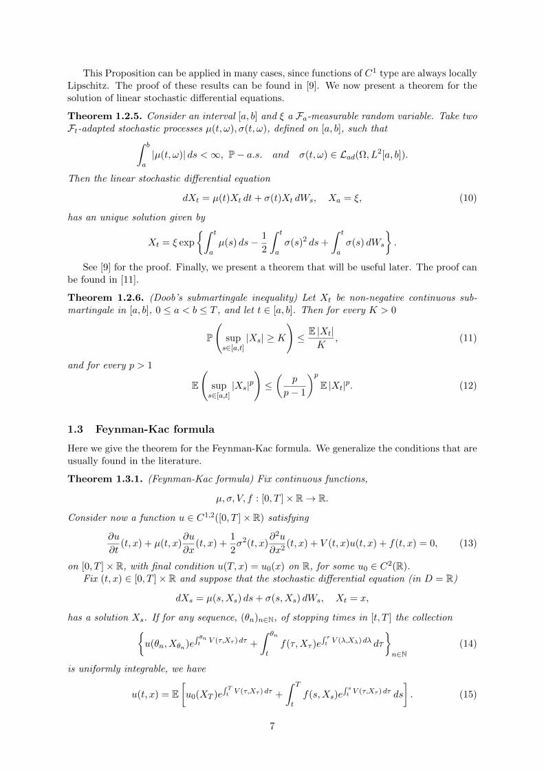
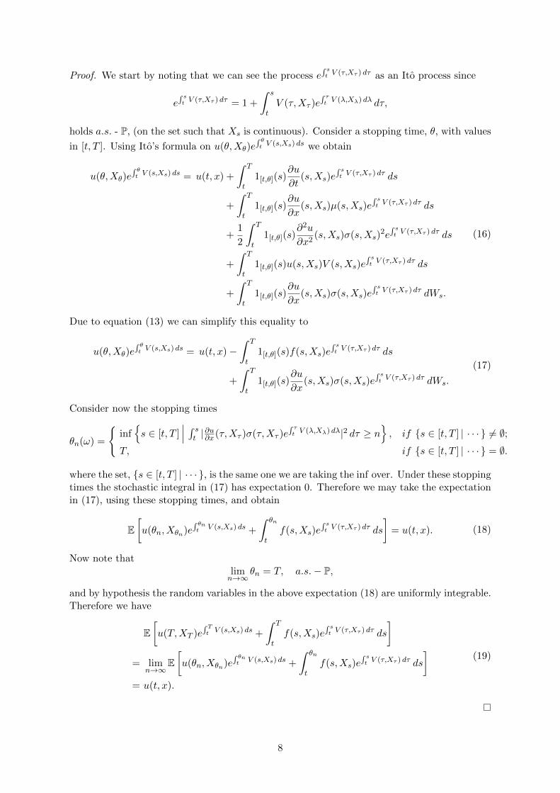
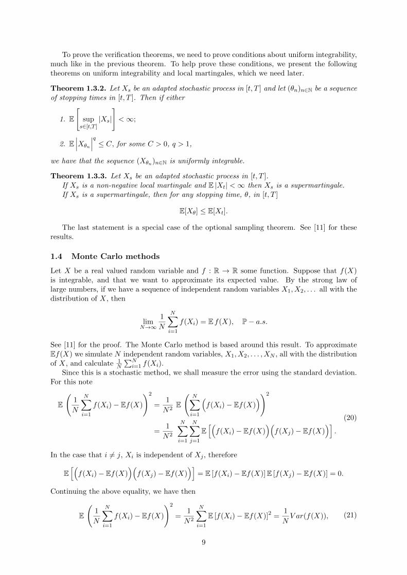
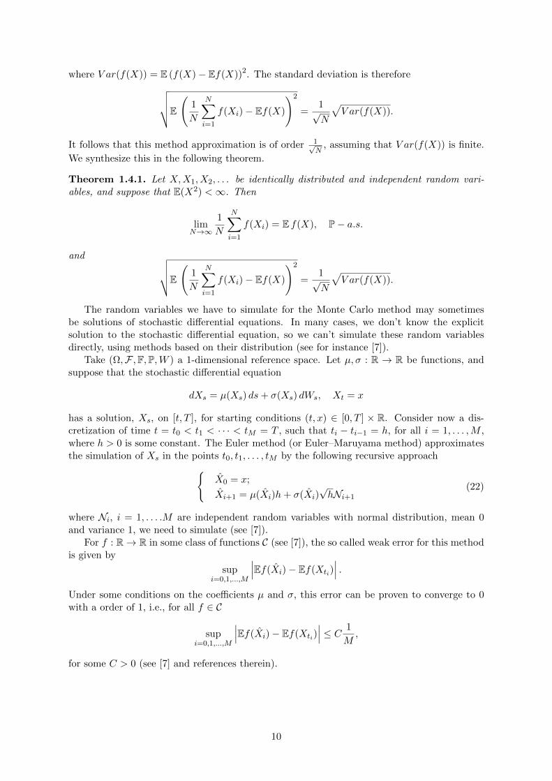
1 Approximation of F (0, 1/2 log(y)) in the Heston model, γ = 0.3 and N = 50. . 452 Approximation of F (0, 1/2 log(y)) in the Heston model, γ = 0.3 and N = 100. . 453 Approximation of F (0, 1/2 log(y)) in the Heston model, γ = 0.9 and N = 50. . 464 Approximation of F (0, 1/2 log(y)) in the Heston model, γ = 0.9 and N = 100. . 465 Approximation of F (t, log(y)) in the 2-hypergeometric model, γ = 0.3 . . . . . 476 Approximation of F (t, log(y)) in the 2-hypergeometric model, γ = 0.9 . . . . . 48

XIII

Acronyms

1. CIR - Cox–Ingersoll–Ross;

2. HJB - Hamilton-Jacobi-Bellman;

XV

Introduction

Ever since the seminal papers by Merton [16, 17], there has been a lot of research on continuous-time portfolio optimization, in the context of stochastic analysis. Merton considers the portfolioproblem for the Black-Scholes model, and solves it in several contexts, for example, lifetimeconsumption and maximizing utility from terminal wealth. In this thesis we focus on thelatter. It is well known that the Black-Scholes model does not describe accurately the realityof financial markets. For instance, it doesn’t capture the volatility smile and skew feature ofimplied volatilities (see for instance the book by Zhu [24]).

To solve these problems, one approach has been to allow the volatility of the stocks to bestochastic, by the introduction of so called stochastic volatility models. Heston [8] proposesa model of this type using the Cox–Ingersoll–Ross process and taking the volatility of thestock to be the square root of this process. This model seems to be the most widely usedtoday among the stochastic volatility models, especially for option pricing. For a model of thistype, Liu, in [15], proposes a solution to the continuous-time portfolio optimization problemfor power utilities, by solving the dynamic programming equations. However, a solution tothese equations may not correspond to the payoff function of the optimal portfolio; in additionone needs to prove a verification theorem (see Kraft [13]). Following the approach by Kraft[13], we generalize his result of verification for general stochastic volatility models and generalutilities.

Concerning the Heston model, if the so called Feller condition is not satisfied, the CIRprocess can reach zero in finite time, and in statistical estimation of the parameters we don’talways have this condition. To overcome these issues, in the recent paper [4], the authorsdevelop a new model, the α-Hypergeometric Stochastic Volatility Model. This model alwayshas a positive distribution for the volatility, and at the same time remains tractable. Thepricing of derivatives under this model has been object of recent research (see [20, 21]). One ofour main goals is to analyse the portfolio problem for this model. More precisely we obtain aFeynman-Kac formula for the solution of the Hamilton-Jacobi-Bellman equation (HJB), whichis the natural candidate to be the payoff of the optimal portfolio. Taking into account thisstochastic representation we develop and implement a Monte Carlo type of numerical schemefor the solution of the HJB equation.

This work is organized as follows. In section 1, we review some results of stochastic analysisthat we need throughout the thesis.

In section 2, we introduce our formulation using the Merton problem, i.e., the portfolioproblem in the Black-Scholes framework. The purpose of this section is to give a general ideaand a motivation to the general approach that we propose for stochastic volatility models.

In section 3, we formulate the general stochastic volatility portfolio problem. Using the con-dition of uniform integrability (like in Kraft [13]), we prove the verification theorem for generalutilities. We also discuss the problem for power utilities, in which the dynamic programmingequations can reduced to a linear differential equation, as proposed in [23].

In section 4, we solve the problem for a family of models that include the Heston modelproposed by Liu [15]. For this family of models, the dynamic programming equations can besolved explicitly, and the conditions of the verification theorem can be proved, ensuring theoptimality of the solution. This section follows closely the paper of Kraft [13].

In section 5, we propose a general method to solving the problem using the Feynman-Kacformula, from a theoretical and numerical point of view. First, we simplify the equation suchthat the corresponding partial differential operator coincides with the infinitesimal generatorof the stochastic volatility model. Then we write the Feynman-Kac formula using the processwith this infinitesimal generator. Such process is appropriate to show that the Feynman-Kacrepresentation is finite valued for any given initial condition. Otherwise, in some cases, if weconsider the original partial differential equation, the associated stochastic process is hard to

1

deal with. In addition it is difficult to show that the Feynman-Kac representation is finitevalued. This strategy can be applied successfully to the 2-hypergeometric model. Finally, stillbased on the deduced representation, we develop and implement a Monte Carlo type of methodto obtain a numerical approximation.

2

1 Elements of Stochastic Analysis and Monte Carlo methods

1.1 Introductory concepts

Throughout this work we shall fix a constant T > 0. In this section, we remind various resultsof stochastic analysis which will be needed later. We start with various definitions.

Definition 1.1.1. Let (Ω,F ,P) be a probability space. A filtration on (Ω,F ,P) is a family,F = (Ft)t∈[0,T ], of σ-algebras such that Fs ⊆ Ft ⊆ F , for any 0 ≤ s ≤ t ≤ T . We say that afiltration is right continuous if

Ft =⋂s>t

Fs ,

for any t ∈ [0, T ).A probability space, (Ω,F ,P), is complete if the set N = A ∈ F |P(A) = 0 satisfies

∀A ∈ N , ∀B ⊆ Ω, B ⊆ A =⇒ B ∈ F .

A filtered probability space satisfying the usual conditions, is an ordered vector, (Ω,F ,F,P),such that (Ω,F ,P) is a probability space, F = (Ft)t∈[0,T ] is a filtration on (Ω,F ,P), and

1. (Ω,F ,P) is a complete probability space;

2. F0 contains all null measure sets of F , i.e., N ⊆ F0;

3. The filtration F = (Ft)t∈[0,T ] is right continuous.

For 0 ≤ a ≤ b ≤ T , a stochastic process in [a, b], is a mapping from [a, b]× Ω into R, suchthat, it’s measurable in the product σ-algebra, B([a, b])×F . We say that a stochastic process in[a, b], X(s, ω), is Ft-adapted if the random variable X(s, ·) is Fs-measurable, for any s ∈ [a, b].

Definition 1.1.2. Take a filtered probability space satisfying the usual conditions (Ω,F ,F,P).A Ft Brownian motion is a stochastic process, (Wt)t∈[0,T ], such that

1. Wt is Ft-adapted;

2. For any 0 ≤ s < t ≤ T , the random variable Wt −Ws, is independent of Fs;

3. W0 = 0 almost surely;

4. For any 0 ≤ s < t ≤ T , Wt −Ws ∼ N(0, t− s);

5. For any 0 ≤ t1 < t2 < · · · < tn ≤ T , the random variables

Wt1 , Wt2 −Wt1 , . . . , Wtn −Wtn−1 ,

are independent.

6. The process Wt is pathwise continuous, i.e., there is A ∈ F with P(A) = 1 such thatW (·, ω) is continuous for all ω ∈ A.

Definition 1.1.3. For a probability space, (Ω,F ,P), n stochastic processes, f1(t), f2(t), . . . , fn(t),are said to be independent if for any 0 ≤ t1 < t2 < · · · < tm ≤ T , the m-valued random variables(f1(t1), f1(t2), . . . , f1(tm)), . . . , (fn(t1), fn(t2), . . . , fn(tm)) are independent.

Given a filtered probability space satisfying the usual conditions (Ω,F ,F,P), we call a q-dimensional Brownian motion, to a mapping from [0, T ]× Ω to Rq, Wt = (W 1

t , . . . ,Wqt ), such

that

1. Each mapping W it is an Ft Brownian motion;

3

2. The stochastic processes, W 1t , . . . ,W

qt , are independent.

A q-dimensional reference space is an ordered vector (Ω,F ,F,P,W ) such that (Ω,F ,F,P) isa filtered probability space satisfying the usual conditions and W is a q-dimensional Brownianmotion.

Given these definitions one can develop the concept of the stochastic integral. We give abrief review of this concept in the following observation. The full development can be found in[14].

Observation 1.1.4. Given a filtered probability space satiffeynmasfying the usual conditions(Ω,F ,F,P) we may take the following spaces of stochastic processes:

1. L2ad([a, b]× Ω) the space of stochastic processes, f(t, ω), such that

(a) f(t, ω) is Ft adapted;

(b) E∫ ba |f(s)|2 ds <∞.

2. Lad(Ω, L2[a, b]) the space of stochastic processes, f(t, ω), such that

(a) f(t, ω) is Ft adapted;

(b)∫ ba |f(s)|2 ds <∞, P-a.s.

We note that L2ad([a, b]× Ω) ⊆ Lad(Ω, L2[a, b]). We know that for a Ft Brownian motion, Wt,

and stochastic process, f ∈ Lad(Ω, L2[a, b]), the stochastic integral∫ ba f(s, ω) dWs is well defined

as an element of L0(Ω). In the particular case that f ∈ L2ad([a, b]× Ω), the stochastic integral∫ b

a f(s, ω) dWs is an element of L2(Ω).

We also know that we can take representatives of∫ ta f(s) dWs, a ≤ t ≤ b, i.e., take elements

of the a.s. equivalence classes of∫ ta f(s) dWs, such that the mapping

(t, ω) 7→∫ t

0f(s) dWs

is a continuous stochastic process (a continuous stochastic process is one that satisfies condition6 of Definition 1.1.2).

We present now the theorem for Ito’s formula. First let’s define what we mean by an Itoprocess.

Definition 1.1.5. Consider a q-dimensional reference space (Ω,F ,F,P,W ). A stochastic pro-cess, Xt, defined on [a, b] is an Ito process if

1. Xt is Ft-adapted and continuous;

2. There exist stochastic processes f(t, ω), σ1(t, ω), . . . , σq(t, ω), such that

(a) f(t, ω) is Ft-adapted and∫ ba |f(t, ω)| ds <∞, P-a.s.;

(b) σi(t, ω) ∈ Lad(Ω, L2[a, b]), 1 ≤ i ≤ q;(c) the equality

Xt = Xa +

∫ t

af(s, ω) ds+

q∑i=1

∫ t

aσi(s, ω) dW i

s (1)

holds a.s., for any t ∈ [a, b].

We present Ito’s formula now, which we generalize for stopping times.

4

Theorem 1.1.6. Take an ito process, Xt, with corresponding stochastic processes f(t, ω),σ1(t, ω), . . . , σq(t, ω) as in the previous definition. Then for any function F : [a, b] × R → R,such that it’s partial derivatives ∂F

∂t , ∂F∂x , ∂2F

∂x2, exist and are continuous, and for any stopping

time, θ, with values in [a, b], the equality

F (θ,Xθ) = F (a,Xa) +

∫ b

a1[a,θ](s)

∂F

∂t(s,Xs) ds+

∫ b

a1[a,θ](s)

∂F

∂x(s,Xs)f(s, ω) ds

+

q∑i=1

∫ b

a1[a,θ](s)

∂F

∂x(s,Xs)σi(s, ω) dW i

s

+1

2

q∑i=1

∫ b

a1[a,θ](s)

∂2F

∂x2(s,Xs)σi(s, ω)2 ds

(2)

holds P-a.s.

We can also generalize this theorem for n dimensions.

Theorem 1.1.7. Take Ito processes, Xit , with corresponding stochastic processes fi(t, ω),

σi,1(t, ω), . . . , σi,q(t, ω), as in the previous definition (1 ≤ i ≤ n). Then for any function

F : [a, b]×Rn → R such that it’s partial derivatives ∂F∂t , ∂F

∂xi, ∂2F∂xixj

, for i, j = 1, . . . , n, exist and

are continuous, and for any stopping time, θ, with values in [a, b], the equality

F (θ,Xθ) = F (a,Xa) +

∫ b

a1[a,θ](s)

∂F

∂t(s,Xs) ds+

n∑i=1

∫ b

a1[a,θ](s)

∂F

∂xi(s,Xs)fi(s, ω) ds

+n∑i=1

q∑j=1

∫ b

a1[a,θ](s)

∂F

∂xi(s,Xs)σij(s, ω) dW j

s

+1

2

n∑i=1

n∑j=1

q∑k=1

∫ b

a1[a,θ](s)

∂2F

∂xixj(s,Xs)σik(s, ω)σjk(s, ω) ds

(3)

holds P-a.s. ( we’re denoting Xt = (X1t , . . . , X

nt ) ).

The proof of these generalized theorems can be done using the usual Ito’s formula and aproperty of stochastic integrals with stopping times (see Friedman [6]).

1.2 Stochastic Differential Equations

Take for now a 1-dimensional reference space (Ω,F ,F,P,W ). A 1-dimensional stochastic dif-ferential equation on the interval [a, b], 0 ≤ a ≤ b ≤ T , and domain D ⊆ R (we always takeD = R or D = R+) is a differential of the form

dXt = µ(t,Xt, ω) dt+ σ(t,Xt, ω) dWt, Xa = ξ. (4)

where µ : [a, b]×D×Ω→ R and σ : [a, b]×D×Ω→ R are given mappings, and ξ is a certainFa-measurable random variable. In a way this differential has no exact mathematical form,it’s simply something we refer to for ease of communication. Let’s define now precisely whatwe mean by a solution of this equation.

Definition 1.2.1. Fix an interval [a, b], domain D ⊆ R, mappings µ, σ : [a, b] ×D × Ω → Rand a Fa-measurable random variable ξ. A solution of the stochastic differential equation (4),is a stochastic process, Xt, defined on [a, b], such that

1. Xt takes values in D, is Ft-adapted, and is continuous;

5

2. µ(t,Xt, ω) is an Ft-adapted process such that∫ ba |µ(s,Xs, ω)| ds <∞ for P-a.s.;

3. σ(t,Xt, ω) ∈ Lad(Ω, L2[a, b]), so the stochastic integral is well defined;

4. The equality

Xt = ξ +

∫ t

aµ(s,Xs, ω) ds+

∫ t

aσ(s,Xs, ω) dWs (5)

holds a.s., for any t ∈ [a, b].

This last equality means that for each fixed t ∈ [a, b], for any version of the stochasticintegral, there is as set A ∈ F with P(A) = 1, such that for all ω ∈ A,

∫ ta |µ(s,Xs, ω)| ds <∞,

so this integral is well defined and the equality (5) holds (for the fixed t and ω).

Definition 1.2.2. We say that the solution to the stochastic differential equation (4) is uniqueif for any two solutions, Xt, Yt, as in definition 1.2.1, satisfy

X(t, ω) = Y (t, ω), for all t ∈ [a, b],

in a set of probability one.

We note that this is stronger then Xt = Yt a.s. for all t ∈ [a, b], i.e. the statement in thedefinition says there is a set of probability one such that the paths of the stochastic processescoincide. Still because the processes are continuous by definition, if Xt = Yt a.s. for all t ∈ [a, b]one will still get the stronger property of pathwise uniqueness. As such, in our case the twoviews are equivalent.

We present the usual theorem of existence and uniqueness of solution with Lipschitz coef-ficients, where the functions µ and σ do not depend on ω

Theorem 1.2.3. Fix an interval [a, b] and take measurable functions µ, σ : [a, b]×R→ R suchthat for some K > 0

|µ(t, x)− µ(t, y)| ≤ K|x− y|, |σ(t, x)− σ(t, y)| ≤ K|x− y|, ∀ t ∈ [a, b], x, y ∈ R, (6)

and for some C > 0

|µ(t, x)| ≤ C(1 + |x|) |σ(t, x)| ≤ C(1 + |x|), ∀t ∈ [a, b], x ∈ R. (7)

Suppose ξ is a Fa measurable random variable such that E(|ξ|2) < ∞. Then the stochasticdifferential equation (4) as an unique solution.

Also a solution to this equation, Xt, satisfies the following estimate

E

(supa≤t≤b

|Xt|2)≤ C E(|ξ|2), (8)

for some C > 0.

We also have the following Proposition for proving the uniqueness of a solution.

Proposition 1.2.4. Fix an interval [a, b] and domain D ⊆ R such that D = R or D = R+.Take a Fa-measurable random variable, ξ, and functions µ, σ : [a, b]×D → R such that for anycompact set K ⊆ D there exists CK > 0 satisfying

|µ(t, x)− µ(t, y)| ≤ CK |x− y|, |σ(t, x)− σ(t, y)| ≤ CK |x− y|, ∀ t ∈ [a, b], x, y ∈ K. (9)

If Xt is a solution of (4), for these mappings, then this solution is unique.

6

This Proposition can be applied in many cases, since functions of C1 type are always locallyLipschitz. The proof of these results can be found in [9]. We now present a theorem for thesolution of linear stochastic differential equations.

Theorem 1.2.5. Consider an interval [a, b] and ξ a Fa-measurable random variable. Take twoFt-adapted stochastic processes µ(t, ω), σ(t, ω), defined on [a, b], such that∫ b

a|µ(t, ω)| ds <∞, P− a.s. and σ(t, ω) ∈ Lad(Ω, L2[a, b]).

Then the linear stochastic differential equation

dXt = µ(t)Xt dt+ σ(t)Xt dWs, Xa = ξ, (10)

has an unique solution given by

Xt = ξ exp

∫ t

aµ(s) ds− 1

2

∫ t

aσ(s)2 ds+

∫ t

aσ(s) dWs

.

See [9] for the proof. Finally, we present a theorem that will be useful later. The proof canbe found in [11].

Theorem 1.2.6. (Doob’s submartingale inequality) Let Xt be non-negative continuous sub-martingale in [a, b], 0 ≤ a < b ≤ T , and let t ∈ [a, b]. Then for every K > 0

P

(sups∈[a,t]

|Xs| ≥ K

)≤ E |Xt|

K, (11)

and for every p > 1

E

(sups∈[a,t]

|Xs|p)≤(

p

p− 1

)pE |Xt|p. (12)

1.3 Feynman-Kac formula

Here we give the theorem for the Feynman-Kac formula. We generalize the conditions that areusually found in the literature.

Theorem 1.3.1. (Feynman-Kac formula) Fix continuous functions,

µ, σ, V, f : [0, T ]× R→ R.

Consider now a function u ∈ C1,2([0, T ]× R) satisfying

∂u

∂t(t, x) + µ(t, x)

∂u

∂x(t, x) +

1

2σ2(t, x)

∂2u

∂x2(t, x) + V (t, x)u(t, x) + f(t, x) = 0, (13)

on [0, T ]× R, with final condition u(T, x) = u0(x) on R, for some u0 ∈ C2(R).Fix (t, x) ∈ [0, T ]× R and suppose that the stochastic differential equation (in D = R)

dXs = µ(s,Xs) ds+ σ(s,Xs) dWs, Xt = x,

has a solution Xs. If for any sequence, (θn)n∈N, of stopping times in [t, T ] the collectionu(θn, Xθn)e

∫ θnt V (τ,Xτ ) dτ +

∫ θn

tf(τ,Xτ )e

∫ τt V (λ,Xλ) dλ dτ

n∈N

(14)

is uniformly integrable, we have

u(t, x) = E[u0(XT )e

∫ Tt V (τ,Xτ ) dτ +

∫ T

tf(s,Xs)e

∫ st V (τ,Xτ ) dτ ds

]. (15)

7

Proof. We start by noting that we can see the process e∫ st V (τ,Xτ ) dτ as an Ito process since

e∫ st V (τ,Xτ ) dτ = 1 +

∫ s

tV (τ,Xτ )e

∫ τt V (λ,Xλ) dλ dτ,

holds a.s. - P, (on the set such that Xs is continuous). Consider a stopping time, θ, with values

in [t, T ]. Using Ito’s formula on u(θ,Xθ)e∫ θt V (s,Xs) ds we obtain

u(θ,Xθ)e∫ θt V (s,Xs) ds = u(t, x) +

∫ T

t1[t,θ](s)

∂u

∂t(s,Xs)e


+

∫ T

t1[t,θ](s)

∂u

∂x(s,Xs)µ(s,Xs)e


+1

2

∫ T

t1[t,θ](s)

∂2u

∂x2(s,Xs)σ(s,Xs)

2e∫ st V (τ,Xτ ) dτ ds

+

∫ T

t1[t,θ](s)u(s,Xs)V (s,Xs)e


+

∫ T

t1[t,θ](s)

∂u

∂x(s,Xs)σ(s,Xs)e

∫ st V (τ,Xτ ) dτ dWs.

(16)

Due to equation (13) we can simplify this equality to

u(θ,Xθ)e∫ θt V (s,Xs) ds = u(t, x)−

∫ T

t1[t,θ](s)f(s,Xs)e


+

∫ T

t1[t,θ](s)

∂u

∂x(s,Xs)σ(s,Xs)e

∫ st V (τ,Xτ ) dτ dWs.

(17)

Consider now the stopping times

θn(ω) =

infs ∈ [t, T ]

∣∣∣ ∫ st |∂u∂x(τ,Xτ )σ(τ,Xτ )e∫ τt V (λ,Xλ) dλ|2 dτ ≥ n

, if s ∈ [t, T ] | · · · 6= ∅;

T, if s ∈ [t, T ] | · · · = ∅.

where the set, s ∈ [t, T ] | · · · , is the same one we are taking the inf over. Under these stoppingtimes the stochastic integral in (17) has expectation 0. Therefore we may take the expectationin (17), using these stopping times, and obtain

E[u(θn, Xθn)e

∫ θnt V (s,Xs) ds +

∫ θn

tf(s,Xs)e


]= u(t, x). (18)

Now note thatlimn→∞

θn = T, a.s.− P,

and by hypothesis the random variables in the above expectation (18) are uniformly integrable.Therefore we have

E[u(T,XT )e

∫ Tt V (s,Xs) ds +

∫ T

tf(s,Xs)e


]= lim

n→∞E[u(θn, Xθn)e

∫ θnt V (s,Xs) ds +

∫ θn

tf(s,Xs)e


]= u(t, x).

(19)

8

To prove the verification theorems, we need to prove conditions about uniform integrability,much like in the previous theorem. To help prove these conditions, we present the followingtheorems on uniform integrability and local martingales, which we need later.

Theorem 1.3.2. Let Xs be an adapted stochastic process in [t, T ] and let (θn)n∈N be a sequenceof stopping times in [t, T ]. Then if either

1. E

[sups∈[t,T ]

|Xs|

]<∞;

2. E∣∣∣Xθn

∣∣∣q ≤ C, for some C > 0, q > 1,

we have that the sequence (Xθn)n∈N is uniformly integrable.

Theorem 1.3.3. Let Xs be an adapted stochastic process in [t, T ].If Xs is a non-negative local martingale and E |Xt| <∞ then Xs is a supermartingale.If Xs is a supermartingale, then for any stopping time, θ, in [t, T ]

E[Xθ] ≤ E[Xt].

The last statement is a special case of the optional sampling theorem. See [11] for theseresults.

1.4 Monte Carlo methods

Let X be a real valued random variable and f : R → R some function. Suppose that f(X)is integrable, and that we want to approximate its expected value. By the strong law oflarge numbers, if we have a sequence of independent random variables X1, X2, . . . all with thedistribution of X, then

limN→∞

1

N

N∑i=1

f(Xi) = E f(X), P− a.s.

See [11] for the proof. The Monte Carlo method is based around this result. To approximateEf(X) we simulate N independent random variables, X1, X2, . . . , XN , all with the distributionof X, and calculate 1

N

∑Ni=1 f(Xi).

Since this is a stochastic method, we shall measure the error using the standard deviation.For this note

E

(1

N

N∑i=1

f(Xi)− Ef(X)

)2

=1

N2E

(N∑i=1

(f(Xi)− Ef(X)

))2

=1

N2

N∑i=1

N∑j=1

E[(f(Xi)− Ef(X)

)(f(Xj)− Ef(X)

)].

(20)

In the case that i 6= j, Xi is independent of Xj , therefore

E[(f(Xi)− Ef(X)

)(f(Xj)− Ef(X)

)]= E [f(Xi)− Ef(X)]E [f(Xj)− Ef(X)] = 0.

Continuing the above equality, we have then

E

(1

N

N∑i=1

f(Xi)− Ef(X)

)2

=1

N2

N∑i=1

E [f(Xi)− Ef(X)]2 =1

NV ar(f(X)), (21)

9

where V ar(f(X)) = E (f(X)− Ef(X))2. The standard deviation is therefore√√√√E

(1

N

N∑i=1

f(Xi)− Ef(X)

)2

=1√N

√V ar(f(X)).

It follows that this method approximation is of order 1√N

, assuming that V ar(f(X)) is finite.

We synthesize this in the following theorem.

Theorem 1.4.1. Let X,X1, X2, . . . be identically distributed and independent random vari-ables, and suppose that E(X2) <∞. Then

limN→∞

1

N

N∑i=1

f(Xi) = E f(X), P− a.s.

and √√√√E

(1

N

N∑i=1

f(Xi)− Ef(X)

)2

=1√N

√V ar(f(X)).

The random variables we have to simulate for the Monte Carlo method may sometimesbe solutions of stochastic differential equations. In many cases, we don’t know the explicitsolution to the stochastic differential equation, so we can’t simulate these random variablesdirectly, using methods based on their distribution (see for instance [7]).

Take (Ω,F ,F,P,W ) a 1-dimensional reference space. Let µ, σ : R → R be functions, andsuppose that the stochastic differential equation

dXs = µ(Xs) ds+ σ(Xs) dWs, Xt = x

has a solution, Xs, on [t, T ], for starting conditions (t, x) ∈ [0, T ] × R. Consider now a dis-cretization of time t = t0 < t1 < · · · < tM = T , such that ti − ti−1 = h, for all i = 1, . . . ,M ,where h > 0 is some constant. The Euler method (or Euler–Maruyama method) approximatesthe simulation of Xs in the points t0, t1, . . . , tM by the following recursive approach

X0 = x;

Xi+1 = µ(Xi)h+ σ(Xi)√hNi+1

(22)

where Ni, i = 1, . . . .M are independent random variables with normal distribution, mean 0and variance 1, we need to simulate (see [7]).

For f : R→ R in some class of functions C (see [7]), the so called weak error for this methodis given by

supi=0,1,...,M

∣∣∣Ef(Xi)− Ef(Xti)∣∣∣ .

Under some conditions on the coefficients µ and σ, this error can be proven to converge to 0with a order of 1, i.e., for all f ∈ C

supi=0,1,...,M

∣∣∣Ef(Xi)− Ef(Xti)∣∣∣ ≤ C 1

M,

for some C > 0 (see [7] and references therein).

10

2 Merton Problem

2.1 Formulation of the Problem

The Merton Problem is the control problem for the Black Scholes Model. The Black Scholesmodel is given by the dynamics

dBt = rBt dt, B0 = 1,

dSt = µSt dt+ σSt dWt, S0 = s0.(23)

where r, µ are non-negative constants with µ ≥ r and σ, s0 are positive. This system has thesolution

Bt = ert

St = s0e(µ− 1

2σ2)t+σWt ,

(24)

where we are considering a 1-dimensional reference space (Ω,F ,F,P,W ).We want to manage portfolios on this model. By a portfolio we mean a pair of adapted

stochastic processes at, bt such that at represents the quantity the holder has of the asset Btat time t and bt represents the quantity of the asset St the holder has at time t. We can thendefine the value of the portfolio at time t to be

Xt = atBt + btSt. (25)

We want to consider portfolios that are self-financed, i.e., portfolios where money is not injectedor taken out. We formalize this condition by supposing that the wealth process Xt satisfies thedynamics

dXt = atdBt + btdSt. (26)

Developing this equality we obtain

dXt = atdBt + btdSt = (atrBt + btµSt) dt+ btσSt dWt. (27)

We also only consider portfolios such that Xt > 0 for all (t, ω) ∈ [0, T ] × Ω. Since in theBlack-Scholes model, prices are always positive this is not too restrictive.

So as to simplify the equation we take ϕt to denote the fraction of the wealth invested inthe stock St, i.e.

ϕt =StbtXt

, and by (25), 1− ϕt =atBtXt

.

So we have simplydXt = (r(1− ϕt)Xt + µϕtXt) dt+ σ ϕtXt dWt, (28)

which doesn’t depend on St, so we can simply look to this equation to formulate the controlproblem.

Definition 2.1.1. We define the set of admissible controls, A(t), defined on t ∈ [0, T ], to bethe set of adapted stochastic processes, ϕ, with domain [t, T ]× Ω, such that∫ T

t|ϕs|2 ds <∞, a.s. (29)

We note that for a fixed ϕs ∈ A(t), the stochastic differential equation (28) has an uniquesolution for any starting position Xt = x > 0 ( using theorem 1.2.5 ). Given t ∈ [0, T ],x ∈ R+ and ϕs ∈ A(t), we denote a corresponding solution to equation (28) by Xt,x,ϕ

s . Alsonote that, since the equation is a linear equation, for starting time x > 0 we always getXt,x,ϕs > 0, ∀s ∈ [t, T ], a.s.

We are now ready to formulate our control problem. For this we need the concept of anutility function.

11

Definition 2.1.2. An utility function is a function U ∈ C2(R+) such that

U(x) ≥ 0, U ′(x) ≥ 0, and U ′′(x) ≤ 0, for all x ∈ R+

The condition U(x) ≥ 0 is equivalent to supposing U is lower bounded, this is because thecontrol problem is equivalent for utilities such that its difference is constant. The conditionU ′(x) ≥ 0 is so the function is increasing, so that the agent prefers more wealth then less, andthe condition U ′′(x) ≤ 0 is so the agent is risk averse.

The objective is now to find the best control with the maximum payoff E[U(Xϕ

T )], for each

starting condition. Let’s define what we mean by the payoff associated to a control.

Definition 2.1.3. Consider the set

D =

(t, x, ϕ)∣∣∣ t ∈ [0, T ], x ∈ R+, ϕ ∈ A(t)

. (30)

For each (t, x, ϕ) ∈ D we fix a corresponding solution Xt,x,ϕs of equation (28). We define the

payoff function, P : D → R ∪ ∞, for the utility function, U , as being

P (t, x, ϕ) = E[U(Xt,x,ϕ

T )]. (31)

By pathwise uniqueness, E[U(Xt,x,ϕ

T )]

is the same for any solution of equation (28) we fix,

so P (t, x, ϕ) doesn’t depend on the considered solution to the stochastic equation. Now wedefine the notion of value function.

Definition 2.1.4. Let P be the payoff function for a certain utility function U . The valuefunction V : [0, T ]× R+ → R ∪ +∞, is defined by

V (t, x) = supϕ∈A(t)

P (t, x, ϕ). (32)

We shall also denote the value function V , by the lower case v.

2.2 Verification theorem

Our objective is to find a control processes, ϕt,x ∈ A(t), for each (t, x) ∈ [0, T ]×R+, such thatP (t, x, ϕt,x) = V (t, x).

One approach is to solve a deterministic differential equation, called the dynamic prog-graming equations, or also the Hamilton-Jacobi-Bellmann equations (HJB). Finding a solutionto these equations is not always easy, and in some cases the equation might not have a smoothsolution, so one has to use weaker notions of solutions to differential equations, like viscositysolutions (we refer to [3, 22] for these concepts). What we shall do now is prove what is calleda Verification theorem. What this theorem gives us, is a guarantee that in the case that wefind a smooth solution to the HJB equations, and one has an additional uniform integrabilitycondition, then one knows that that solution is the value function.

We start with a Lemma.

Lemma 2.2.1. Let U ∈ C2(R+) be an utility function and let w ∈ C1,2([0, T ] × R+) be anon-negative function satisfying

1. for fixed (t, x) ∈ [0, T ]× R+, the mapping,

a→[∂w

∂x(t, x)x (r + a(µ− r)) +

1

2

∂2w

∂x2(t, x)x2σ2a2

]is bounded above for a ∈ R;

12

2. −∂w∂t

(t, x)− supa∈R

[∂w

∂x(t, x)x (r + a(µ− r)) +

1

2

∂2w

∂x2(t, x)x2σ2a2

]≥ 0, on [0, T ]× R+;

3. w(T, x) ≥ U(x), ∀x ∈ R+.

Then w ≥ v on [0, T ]× R+.

Proof. Let (t, x, ϕ) ∈ D, and take a corresponding solution Xt,x,ϕs . Since w ∈ C1,2([0, T ] ×R+)

we may apply ito’s formula on w(θ,Xt,x,ϕθ ) for any stopping time θ ∈ [t, T ]. Doing this we

obtain

w(θ,Xt,x,ϕθ ) = w(t, x) +

∫ T

t1[t,θ](s)

[∂w

∂t(s,Xt,x,ϕ

s ) +∂w

∂x(s,Xt,x,ϕ

s )Xt,x,ϕs (r + ϕs(µ− r))

]ds

+1

2

∫ T

t1[t,θ](s)

∂2w

∂x2(s,Xt,x,ϕ

s )(Xt,x,ϕs

)2σ2ϕ2

s ds

+

∫ T

t1[t,θ](s)

∂w

∂x(s,Xt,x,ϕ

s )Xt,x,ϕs σϕs dWs,

(33)

a.s.-P. We define the stopping time, θn, for n ∈ N, and valued in [t, T ], by

θn(ω) =

infs ∈ [t, T ]

∣∣∣ ∫ st |∂w∂x (u,Xt,x,ϕu )Xt,x,ϕ

u σϕu|2 du ≥ n, if s ∈ [t, T ] | · · · 6= ∅;

T, ifs ∈ [t, T ] | · · · = ∅,

where s ∈ [t, T ] | · · · refers to the same set we’re taking the inf over.For this stopping time the last term in (33) has expectation 0. On the other hand we have

∂w

∂t(s,Xt,x,ϕ

s ) +∂w

∂x(s,Xt,x,ϕ

s )Xt,x,ϕs (r + ϕs(µ− r)) ds

+1

2

∂2w

∂x2(s,Xt,x,ϕ

s )(Xt,x,ϕs

)2σ2ϕ2

s

≤ ∂w

∂t(s,Xt,x,ϕ

s ) + supa∈R

∂w

∂x(s,Xt,x,ϕ

s )Xt,x,ϕs (r + a(µ− r)) ds

+1

2

∂2w

∂x2(s,Xt,x,ϕ

s )(Xt,x,ϕs

)2σ2a2

≤ 0,

(34)

by condition 2.Given all these observations, taking the expectation in (33) and using inequality (34), we

haveE[w(θn, X

t,x,ϕθn

)]≤ w(t, x). (35)

Now, noting that limn→∞ θn(ω) = T , a.s.-P, and as a result

limn→∞

w(θn, Xt,x,ϕθn

) = w(T,Xt,x,ϕT ),

a.s.-P, we can use Fatou’s Lemma to obtain

P (t, x, ϕ) = E[U(Xt,x,ϕ

T )]≤ E

[w(T,Xt,s,ϕ

T )]≤ lim inf

n→∞E[w(θn, X

t,x,ϕθn

)]≤ w(t, x). (36)

We note that we can indeed use Fatou’s Lemma because w is a non-negative function. Finally,by taking the sup over ϕ ∈ A(t) in the last inequality, we obtain

v(t, x) ≤ w(t, x).

13

We note that if we find w in the above conditions we also prove that the value function isalways finite. We present now the Verification theorem.

Theorem 2.2.2. (Verification theorem) Let U be an utility function and let w ∈ C1,2([0, T ] ×R+) be a non-negative function satisfying

1. for fixed (t, x) ∈ [0, T ]× R+, the mapping,

a→[∂w

∂x(t, x)x (r + a(µ− r)) +

1

2

∂2w

∂x2(t, x)x2σ2a2

]is bounded above for a ∈ R;

2. −∂w∂t

(t, x)− supa∈R

[∂w

∂x(t, x)x (r + a(µ− r)) +

1

2

∂2w

∂x2(t, x)x2σ2a2

]= 0, on [0, T ]× R+;

3. w(T, x) = U(x), ∀x ∈ R+.

Let α : [0, T ]× R+ → R be a function such that

α(t, x) ∈ arg maxa∈R

∂w

∂x(t, x)x (r + a(µ− r)) +

1

2

∂2w

∂x2(t, x)x2σ2a2

, on [0, T ]× R+ (37)

(such a function always exists by condition 1). If for (t, x) ∈ [0, T ]× R+ the equation

dXt,xs = Xt,x

s (r + α(s, Xt,xs )(µ− r)) ds+ Xt,x

s σα(s, Xt,xs ) dWs, Xt,x

t = x, (38)

has a solution, Xt,xs , with α(s, Xt,x

s ) ∈ A(t) and if for any sequence, (τn)n∈N, of stopping timesin [t, T ] the collection

w(τn, Xt,xτn )n∈N

, (39)


w(t, x) = P (t, x, α(s, Xt,xs )) = v(t, x).

Proof. By the last Lemma it’s immediate that w ≥ v on [0, T ]×R+. Fix now (t, x) ∈ [0, T ]×R+.

If we denote ϕ∗s = α(s, Xt,xs ) it should be immediate that Xt,x

s = Xt,x,ϕ∗s for all s ∈ [t, T ], P-a.s.

This is true since they both satisfy equation (28) for the control ϕ∗s.We take the same stopping times, θn, as in last Lemma and in an analogous argumentation,

we may take Ito’s formula on the process w(θn, Xt,x,ϕ∗

θn) to obtain

E[w(θn, X

t,x,ϕ∗

θn)]

= w(t, x),

where this time we have equality, by the stronger conditions on the function w, and the factthat α(t, x) satisfies condition (37). Now since

limn→∞

θn = T, a.s.− P,

andw(θn, X

t,xθn

)n∈N

is uniformly integrable by hypothesis, we have

v(t, x) ≥ E[U(Xt,x,ϕ∗

T )]

= E[w(T,Xt,x,ϕ∗

T )]

= limn→∞

E[w(θn, X

t,x,ϕ∗

θn)]

= w(t, x). (40)

Since w ≥ v on [0, T ]× R+ we have then

w(t, x) = v(t, x)

and since also w(t, x) = E[U(Xt,x,ϕ∗

T )], α(s, Xt,x

s ) is an optimal control.

14

We remind that to prove that for any sequence of stopping times, (τn)n∈N, the collectionw(τn, X

t,xτn )n∈N

,

is uniformly integrable we can simply prove

E

[sups∈[t,T ]

|w(s, Xt,xs )|

]<∞, or E

[w(τn, X

t,xτn )q

]≤ C,

for some q > 1 and C > 0, which should be easier.

2.3 Power utility functions

In this section we investigate a special type of utility functions.

Definition 2.3.1. An utility function, U , is said to be of power utility type if there existsγ ∈ ]0, 1[ such that

U(x) =xγ

γ

There’s meaning for this type of utilities and we refer to Pham [18] for a discussion (theyhave what is called constant relative risk aversion ).

These utilities are interesting because the HJB equation, in the Merton problem, admits asmooth solution, and this solution can be proved to be optimal using the verification theorem.

The HJB equation is given by−∂w∂t

(t, x)− supa∈R

[∂w

∂x(t, x)x (r + a(µ− r)) +

1

2

∂2w

∂x2(t, x)x2σ2a2

]= 0, on [0, T ]× R+,

w(T, x) = xγ/γ.

(41)Suppose now that this equation has a smooth solution, w, which admits a decomposition ofthe form w(t, x) = h(t)x

γ

γ , with h(t) > 0 for all t ∈ [t, T ]. Substituting in the equation we get−∂h∂t

(t, x)xγ

γ− sup

a∈R

[h(t)xγ (r + a(µ− r)) +

1

2h(t)xγ(γ − 1)σ2a2

]= 0, on [0, T ]× R+,

h(T ) = 1.

(42)Now the supremum is taken over a second order polynomial, so it achieves its maximum if

its highest order coefficient is negative. We can see this is the case since h(t) > 0 and γ ∈]0, 1[.Taking the derivative we can find that this polynomial achieves it’s maximum in

a∗ =µ− r

(1− γ)σ2.

Dividing the equation by xγ/γ and using this maximum, the equation simplifies to−∂h∂t

(t, x)− h(t)γ

(r +

1

2

(µ− r)2

(1− γ)σ2

)= 0, on [0, T ]× R+,

h(T ) = 1.

(43)

15

Denoting by η = γ(r + 1

2(µ−r)2(1−γ)σ2

)we conclude that

h(t) = eη(T−t).

This suggests that in this problem v(t, x) = eη(T−t) xγ

γ . We shall use the verification theoremto prove this.

Proposition 2.3.2. For the utility U(x) = xγ/γ, the value function of the associated Mertoncontrol problem is given by

w(t, x) = eη(T−t)xγ

γ,

where η = γ(r + 1

2(µ−r)2(1−γ)σ2

), and an optimal control is given by

ϕ∗(s, ω) =µ− r

(1− γ)σ2

for any starting conditions t ∈ [0, T ], x ∈ R+.

Proof. Firstly, to prove that w satisfies conditions 1,2 and 3 of the verification theorem simplyfollow the steps we did before, backwards. One can also check that

µ− r(1− γ)σ2

∈ arg maxa∈R

∂w

∂x(t, x)x (r + a(µ− r)) +

1

2

∂2w

∂x2(t, x)x2σ2a2

,

for any (t, x) ∈ [0, T ]× R+. Define α(t, x) = µ−r(1−γ)σ2 on [0, T ]× R+.

Fix starting conditions (t, x) ∈ [0, T ] × R+. Then, α(s, x) being constant, equation (38)always has a solution, Xt,x

s and α(s, Xt,xs ) ∈ A(t). Now lets check that

E

[sups∈[t,T ]

|w(s, Xt,xs )|

]<∞,

which, as we have noted, will imply the condition in the verification theorem. Firstly we notethe following. For a Brownian motion, Ws − Wt (starting at t), the process e|C(Ws−Wt)| isa non-negative submartingale for any C ∈ R, since x 7→ e|Cx| is convex and the process isintegrable. Therefore we can use Doob’s submartingale inequality to conclude

E sups∈[t,T ]

e|C(Ws−Wt)| ≤

(E sups∈[t,T ]

[e|C(Ws−Wt)|

]2)1/2

≤ 2

(E[e|C(WT−Wt)|

]2)1/2

<∞.

Denote α(t, x) simply by α. We have

w(s, Xt,xs ) = eη(T−s)

(Xt,xs )γ

γ

= eη(T−s)(x exp

r(s− t) + α(µ− r)(s− t)− 1

2σ2α2(s− t) + σα(Ws −Wt)

)γ

γ

≤ xγ

γe|C(T−t)|e|γσα(Ws−Wt)|

(44)

where C is some constant. It follows that

E

[sups∈[t,T ]

|w(s, Xt,xs )|

]≤ xγ

γe|C(T−t)| E

[sups∈[t,T ]

e|γσα(Ws−Wt)|

]<∞.

Therefore, using the verification theorem, w(t, x) = v(t, x) and α is an optimal control.

16

3 Stochastic Volatility

3.1 Stochastic volatility models

In this section we fix a 2-dimensional reference space (Ω,F ,F,P,W ) and a constant ρ ∈ [−1, 1].We define a new Brownian motion W ∗t = ρW 1

t +√

1− ρ2W 2t , so that the correlation between

W ∗t and W 1t is ρ.

We now generalize the Black-Scholes model by adding an extra stochastic process, andletting the mean and the volatility of the stock be functions of it. For the extra stochasticdifferential equation we shall always consider its domain D = R. Take continuous mappingsA,B : R→ R. Suppose that for these mappings the stochastic differential equation

dZs = B(Zs) ds+A(Zs) dW∗s , Zt = z, (45)

has a solution for any starting time t ∈ [0, T ] and initial condition z ∈ R. Our new stochasticvolatility market model will be the following system of stochastic differential equations

dBs = rBs ds,

dSs = µ(Zs)Ss ds+ eZsSs dW1s ,

dZs = B(Zs) ds+A(Zs) dW∗s ,

(46)

where r ≥ 0 and µ : R→ R is a continuous function.We have generalized the notion of a stochastic volatility model so the volatility process is

always the exponential of the extra process. This is always possible if one does the appropriatetransformations. For instance if the volatility was of the form σ(Ys), for some process Ys, withan associated stochastic differential equation, and σ, a bijective positive function, we can alwaystake Zs = log(σ(Ys)) and find the equation for Zs by applying Ito’s formula on log(σ(Ys)) andsubstituting Ys by σ−1(eZs).

There are many examples of stochastic volatility models. For instance there is the popularHeston model, which corresponds to the case

dBt = rBt dt,

dSt = µ(Yt)St dt+√YtSt dW

1t ,

dYt = κ(θ − Yt) dt+ α√Yt dW

∗t ,

(47)

where µ is some continuous function, and κ, θ, α are non-negative constants satisfying

2κθ > α2,

the so called Feller condition. The equation of Yt is over R+, because we have assumed theFeller condition, so to get to the form we have presented before we take Zs = log(

√Ys) which

if one applies the Ito formula and substitutes Yt by e2Zt we have the stochastic differentialequation

dZt =

[1

4(2κθ − α2)e−2Zt − 1

2κ

]dt+

1

2αe−Zt dW ∗t .

We end this section by giving a rigorous definition of what is a stochastic volatility model.

Definition 3.1.1. A stochastic volatility model is an ordered vector (A,B, µ), whereµ : R → R is a continuous mapping, and A,B : R → R are continuous mappings, such thatA(z) 6= 0 for all z ∈ R, and the stochastic differential equation

dZs = B(Zs) ds+A(Zs) dW∗s , Zt = z, (48)

has an unique solution over [t, T ], for any starting conditions (t, z) ∈ [0, T ]× R.

We could take A(z) to be always positive since if one finds a model where A(z) is negativewe can take a different Brownian motion where the correlation is −ρ. To avoid having to makethese transformations we present this definition this way.

17

3.2 Formulation of the problem and the verification theorem

We fix now a stochastic volatility model (A,B, µ). For the formulation of the control problem,we can follow a similar approach as the one we did in the Merton problem. Fix (t, z) ∈ [0, T ]×Rand Zs the solution to (48) for these starting conditions. Following the same steps as in theMerton problem, considering only self-financed portfolios where the wealth process remainspositive and representing by ϕs the fraction of our wealth invested in the stock, we get thestochastic differential equation for the wealth process

dXs = (r + (µ(Zs)− r)ϕs)Xs ds+ eZsϕsXs dW1s , Xt = x, (49)

for starting condition x > 0. Since µ is continuous and so is Zs, this linear stochastic differentialequation has a solution has long as∫ T

tϕ(s, ω) ds <∞, a.s.− P

So it makes sense to define the set of admissible controls in the same way as in the Mertonproblem. We give the definition again for easy reference .

Definition 3.2.1. We define the set of admissible controls, A(t), defined on t ∈ [0, T ], to bethe set of adapted stochastic processes, ϕ, with domain [t, T ]× Ω, such that∫ T

t|ϕs|2 ds <∞, a.s. (50)

One can note that by supposing that the admissible controls are adapted stochastic pro-cesses, they can be processes of the form α(s, Zs), and so we’re in a sense supposing that thevolatility is perfectly observable, which is not entirely realistic. Yet one can use implied volatil-ities wich is actually observable and infer the value of the instantaneous volatility. Anotherpossibility can be to use high frequency data ( we refer to [1] for this ).

We use the same concept for utility functions as before

Definition 3.2.2. An utility function is a function U ∈ C2(R+) such that

U(x) ≥ 0, U ′(x) ≥ 0, and U ′′(x) ≤ 0, for all x ∈ R+

We can now give the definitions of the Payoff function and the value function, which areslightly different then the Merton problem.

Definition 3.2.3. For each (t, z) ∈ [0, T ]×R we correspond a process, Zt,zs , which is a solutionof equation (48) for starting conditions (t, z). Consider now the set

G =

(t, x, z, ϕ)∣∣∣ t ∈ [0, T ], x ∈ R+, z ∈ R, ϕ ∈ A(t)

. (51)

For each (t, x, z, ϕ) ∈ G we correspond a process, Xt,x,z,ϕs , which is a solution of the equation

dXt,x,z,ϕs = (r + (µ(Zt,zs )− r)ϕs)Xt,x,z,ϕ

s ds+ eZt,zs ϕsX

t,x,z,ϕs dW 1

s , Xt,x,z,ϕt = x, (52)

Definition 3.2.4. We define the payoff function, P : G → R ∪ +∞, for the utility functionU , to be

P (t, x, z, ϕ) = E[U(Xt,x,z,ϕ

T )], (53)

and the value function V : [0, T ]× R+ × R→ R ∪ +∞ to be

V (t, x, z) = supϕ∈A(t)

P (t, x, z, ϕ). (54)

We also denote the value function V by the lower case v.

18

Once again, one can prove that the payoff is uniquely defined for any of the mappings wetake, since the solutions of the stochastic differential equations are pathwise unique.

Our objective is, for each (t, x, z) ∈ [0, T ] × R+ × R, find a control ϕs ∈ A(t) such thatP (t, x, z, ϕ) = V (t, x, z). For this we develop the HJB equations. We shall now prove theVerification theorem, as was done for the Merton problem. We start with a Lemma.

Lemma 3.2.5. Let w ∈ C1,2([0, T ] × (R+ × R)) be a non-negative function, and let U be anutility function. Suppose that

1. for fixed (t, x, z) ∈ [0, T ] × R+ × R , the mapping

a→[∂w

∂xx(r + a(µ(z)− r)) +

∂2w

∂x∂zaezxA(z)ρ+

1

2

∂2w

∂x2e2za2x2

],

is bounded above for a ∈ R;

2. w satisfies the inequality

−∂w∂t− ∂w

∂zB(z)− 1

2

∂2w

∂z2(t, x, z)A(z)2

− supa∈R

[∂w

∂xx(r + a(µ(z)− r)) +

∂2w

∂x∂zaezxA(z)ρ+

1

2

∂2w

∂x2e2za2x2

]≥ 0

(55)

in [0, T ] × R+ × R;

3. w(T, x, z) ≥ U(x), ∀(x, z) ∈ R+ × R.Then w ≥ v on [0, T ]× R+ × R.

Proof. Let (t, x, z, ϕ) ∈ G. Take Zt,zs , the solution to equation (48) for starting conditions(t, z), and Xt,x,z,ϕ

s , as in definition 3.2.3. Consider a stopping time θ with values in [t, T ]. Sincew ∈ C1,2([0, T ] × (R+ × R)) we may apply Ito’s formula on w(θ,Xt,x,z,ϕ

θ , Zt,zθ ) and obtain

w(θ,Xt,x,z,ϕθ , Zt,zθ ) = w(t, x, z) +

∫ T

t1[t,θ](s)

∂w

∂t(· · · ) ds

+

∫ T

t1[t,θ](s)

∂w

∂x(· · · )Xt,x,z,ϕ

s (r + (µ(Zt,zs )− r)ϕs) ds

+

∫ T

t1[t,θ](s)

∂w

∂z(· · · )B(Zt,zs ) ds

+1

2

∫ T

t1[t,θ](s)

∂2w

∂x2(· · · )

(Xt,x,ϕs

)2 (ϕse

Zt,zs)2

ds

+

∫ T

t1[t,θ](s)

∂2w

∂x∂z(· · · )Xt,x,ϕ

s eZt,zs ϕsA(Zt,zs ) ρ ds

+1

2

∫ T

t1[t,θ](s)

∂2w

∂z2(· · · )

(A(Zt,zs )

)2ds

+

∫ T

t1[t,θ](s)

∂w

∂x(· · · )Xt,x,ϕ

s eZt,zs ϕs dW

1s

+

∫ T

t1[t,θ](s)

∂w

∂z(· · · )A(Zt,zs ) dW ∗s

(56)

a.s.-P, where the ”(· · · )” are abbreviations for (s,Xt,x,z,ϕs , Zt,zs ). We define the stopping time,

θn, for n ∈ N, and valued in [t, T ], by

θn(ω) =

infs ∈ [t, T ]

∣∣∣ ∫ st |∂w∂x (· · · )Xt,x,z,ϕu eZ

t,zu ϕu|2 du ≥ n

∨∫ st |

∂w∂z (· · · )A(Zt,zu )|2 du ≥ n

, if s ∈ [t, T ] | · · · 6= ∅;

T, ifs ∈ [t, T ] | · · · = ∅.

19

Then for these stopping times, the stochastic integrals terms in (56) have expectation 0. Onthe other hand we have, by condition 2

∂w

∂t(· · · ) +

∂w

∂x(· · · )Xt,x,z,ϕ

s (r + (µ(Zt,zs )− r)ϕs) +∂w

∂z(· · · )B(Zt,zs )

+1

2

∂2w

∂x2(· · · )

(Xt,x,ϕs

)2 (ϕse

Zt,zs)2

+∂2w

∂x∂z(· · · )Xt,x,ϕ

s ϕseZt,zs A(Zt,zs )ρ

+1

2

∂2w

∂z2(· · · )

(A(Zt,zs )

)2≤ ∂w

∂t(· · · ) +

∂w

∂z(· · · )B(Zt,zs ) +

1

2

∂2w

∂z2(· · · )

(A(Zt,zs )

)2+ sup

a∈R

∂w

∂x(· · · )Xt,x,z,ϕ

s (r + (µ(Zt,zs )− r) a) +1

2

∂2w

∂x2(· · · )

(Xt,x,ϕs

)2a2e2Z

t,zs

+∂2w

∂x∂z(· · · ) aXt,x,ϕ

s eZt,zs A(Zt,zs )ρ

≤ 0

(57)

for each fixed s ∈ [t, T ] and ω ∈ Ω.Given all these observations, taking the expectation in (56) for θn, we have

E[w(θn, X

t,x,z,ϕθn

, Zt,zθn )]≤ w(t, x, z). (58)

Since w is a continuous non-negative function and limn→∞ θn = T , a.s.-P, we may use Fatou’sLemma to obtain

E[U(Xt,x,z,ϕ

T )]≤ E

[w(T,Xt,s,z,ϕ

T , Zt,zT )]≤ lim inf

n→∞E[w(θn, X

t,x,z,ϕθn

, Zt,zθn )]≤ w(t, x, z). (59)

This holds for all controls, so by taking the sup in ϕ ∈ A(t), we have

V (t, x, z) ≤ w(t, x, z),

We present now the verification theorem.

Theorem 3.2.6. (Verification theorem) Let w ∈ C1,2([0, T ] × (R+ × R)) be a non-negativefunction and let U be an utility function. Suppose that

1. for fixed (t, x, z) ∈ [0, T ] × R+ × R , the mapping

a→[∂w

∂xx(r + a(µ(z)− r)) +

∂2w

∂x∂zaezxA(z)ρ+

1

2

∂2w

∂x2e2za2x2

],

is bounded above for a ∈ R;

2. w satisfies the equality

−∂w∂t− ∂w

∂zB(z)− 1

2

∂2w

∂z2(t, x, z)A(z)2

− supa∈R

[∂w

∂xx(r + a(µ(z)− r)) +

∂2w

∂x∂zaezxA(z)ρ+

1

2

∂2w

∂x2e2za2x2

]= 0

(60)

in [0, T ] × R+ × R;

3. w(T, x, z) = U(x), ∀(x, z) ∈ R+ × R.

20

Let α : [0, T ]× R+ × R→ R be a function such that

α(t, x, z) ∈ arg maxa∈R

∂w

∂xx(r + a(µ(z)− r)) +

∂2w

∂x∂zaezxA(z)ρ+

1

2

∂2w

∂x2e2za2x2

, (61)

on [0, T ] × R+ × R (such a function always exists by condition 1).For (t, x, z) ∈ [0, T ] × R+ × R consider Zt,zs , as in definition 3.2.3, and suppose that the

equation

dXt,x,zs = (r + (µ(Zt,zs )− r)α(t, Xt,x,z

s , Zt,zs ))Xt,x,zs ds+ eZ

t,zs α(t, Xt,x,z

s , Zt,zs )Xt,x,zs dW 1

s , (62)

has a solution, Xt,x,zs , on [t, T ] with starting value x. If α(t, Xt,x,z

s , Zt,zs ) ∈ A(t) and for anysequence, (τn)n∈N, of stopping times in [t, T ] the collection

w(τn, Xt,x,zτn , Zt,zτn )

n∈N

(63)


w(t, x, z) = P (t, x, z, α(s, Xt,x,zs , Zt,zs )) = v(t, x, z).

Proof. By the last Lemma it’s immediate that w ≥ v on [0, T ] × R+ × R. Fix now (t, x, z) ∈[0, T ]×R+×R. Denote by ϕ∗s = α(s, Xt,x,z

s , Zt,zs ). It should be immediate that Xt,x,zs = Xt,x,z,ϕ∗

s

for all s ∈ [t, T ], a.s.-P, using the pathwise uniqueness property of linear stochastic differentialequations.

In an analogous argumentation as in last Lemma, we may take Ito’s formula on the processw(θn, X

t,x,z,ϕ∗

θn, Zt,zθn ), where θn is the same stopping time as in the Lemma, and obtain

E[w(θn, X

t,x,z,ϕ∗

θn, Zt,zθn )

]= w(t, x, z),

for s ∈ [t, T ], where this time we have the equality by the stronger conditions on the functionw and condition (61) on α.

Now sincelimn→∞

θn = T, a.s.− P,

and by hypothesis the collection w(θn, X

t,x,zθn

, Zt,zθn )n∈N


E[U(Xt,x,z,ϕ∗

T )]

= E[w(T,Xt,x,z,ϕ∗

T , Zt,zT )]

= limn→∞

E[w(θn, X

t,x,z,ϕ∗

θn, Zt,zθn )

]= w(t, x, z). (64)

Since we have always v(t, x, z) ≥ P (t, x, z, ϕ∗) it follows that v(t, x, z) ≥ w(t, x, z). But we alsohave w ≥ v on [0, T ]× R+ × R, therefore

w(t, x, z) = v(t, x, z)

and since E[U(Xt,x,z,ϕ∗

T )]

= w(t, x, z) we have that α(s, Xt,x,zs , Zt,zs ) is an optimal control.

Our proof of the verification theorems is inspired by the one done by Pham [19] for the casewhere the control equation is Lipschitz. Kraft [13] proves the Lemma in a quicker way usingproperties of local martingales, but for the full Verification theorem he needs to use stoppingtimes like here. We have decided to present the proof this way because it seems simpler.

21

3.3 Power utilities in stochastic volatility models

We shall now consider power utilities, i.e., the case U(x) = xγ

γ for some γ ∈ ]0, 1[. For theseutilities the HJB equation will simplify to a linear equation. This result is due to Zariphopoulou[23].

First we note the following

v(t, x, z) = supϕ∈A(t)

E[(Xt,x,z,ϕT

)γ /γ]

=1

γsup

ϕ∈A(t)E[(xe(··· )

)γ]=xγ

γsup

ϕ∈A(t)E[(e(··· )

)γ],

i.e., the value function for these utilities always has the form xγ

γ G(t, z), where G : [0, T ]×R→R+ is a positive function (we suppose the above sup is finite).

The HJB equation for the stochastic volatility problem is

−∂w∂t− ∂w

∂zB(z)− 1

2

∂2w

∂z2A(z)2

− supa∈R

[∂w

∂xx(r + a(µ(z)− r)) +

∂2w

∂x∂zaezxA(z)ρ+

1

2

∂2w

∂x2e2za2x2

]= 0,

(65)

on [0, T ]×R+×R, with final condition w(T, x, z) = xγ/γ on R+×R. Suppose that this equationhas smooth solution, w, and that it admits a decomposition of the form w = G(t, z)xγ/γ whereG(t, z) ∈ C1,2([0, T ]×R) is a positive function. Rewriting the above equation in terms of G(t, z)we get

−∂G∂t− ∂G

∂zB(z)− 1

2

∂2G

∂z2A(z)2

− γ supa∈R

[G(t, z)(r + a(µ(z)− r)) +

∂G

∂zaezA(z)ρ+

1

2G(t, z)(γ − 1)e2za2

]= 0,

(66)

on [0, T ] × R, with G(T, z) = 1 on R. Since G(t, z) > 0 the above supremum always achievesits maximum, because the coefficient of a2 will always be negative. Applying the derivative ona we find this maximum to be

a∗ =µ(z)− r

(1− γ)e2z+

A(z)ρ

(1− γ)ez∂G

∂z

1

G(t, z)

for each t ∈ [0, T ], z ∈ R. So the equation simplifies to

∂G

∂t+∂G

∂zB(z) +

1

2

∂2G

∂z2A(z)2 +G(t, z) r γ

+1

2G(t, z)

γ(µ(z)− r)2

(1− γ)e2z+∂G

∂z

γ(µ(z)− r)A(z)ρ

(1− γ)ez+

1

2

γ (A(z))2 ρ2

(1− γ)

(∂G

∂z

)2 1

G(t, z)= 0.

(67)

This, being non-linear, is not easily solvable. We shall transform it into a linear equation byconsidering a transformation of the form G(t, z) = H(t, z)η, for some η > 0. Writing theequation in terms of H(t, z) we have

ηHη−1∂H

∂t+ ηHη−1∂H

∂zB(z) +

1

2

(η(η − 1)Hη−2

(∂H

∂z

)2

+ ηHη−1∂2H

∂z2

)A(z)2 + γrHη

+1

2Hη γ(µ(z)− r)2

(1− γ)e2z+ ηHη−1∂H

∂z


(1− γ)ez+

1

2η2Hη−2

(∂H

∂z

)2 γA(z)2ρ2

(1− γ)= 0.

(68)

22

Adding the terms with Hη−2(∂H

∂z

)2

we get

1

2Hη−2

(∂H

∂z

)2

A(z)2(η(η − 1) + η2

γρ2

(1− γ)

).

This suggest taking η so that η(η − 1) + η2γρ2

(1− γ)= 0, which corresponds to

η =1− γ

1− γ + γρ2.

So, taking this η in equation (68) and multiplying by 1ηH

1−η we have

∂H

∂t+∂H

∂zB(z) +

1

2

∂2H

∂z2A(z)2 +

γr

ηH

+1

2Hγ(µ(z)− r)2

η(1− γ)e2z+∂H

∂z


(1− γ)ez= 0.

(69)

Finally, we introduce the transformation

H(t, z) = eγrη(T−t)

F (t, z)

which, writing the above equation in terms of F , one gets

∂F

∂t+∂F

∂zB(z) +

1

2

∂2F

∂z2A(z)2 +

1

2Fγ(µ(z)− r)2

η(1− γ)e2z+∂F

∂z


(1− γ)ez= 0. (70)

It follows that finding a solution to the HJB equation is equivalent to finding a solution tothis linear differential equation. We have then a simpler Verification theorem for these utilityfunctions.

We present now the Verification theorem for these utilities.

Theorem 3.3.1. (Verification theorem for power utility functions) Let γ ∈ ]0, 1[, and define

η =1− γ

1− γ + γρ2.

Let F ∈ C1,2([0, T ]× R) be a positive function satisfying

∂F

∂t+∂F

∂zB(z) +

1

2

∂2F

∂z2A(z)2 +

1

2Fγ(µ(z)− r)2

η(1− γ)e2z+∂F

∂z


(1− γ)ez= 0, (71)

on [0, T ]× R and F (T, z) = 1 on R.Let α : [0, T ]× R→ R be the function defined by

α(t, z) =µ(z)− r

(1− γ)e2z+

ηρA(z)

(1− γ)ez1

F (t, z)

∂F

∂z(t, z). (72)

For (t, x, z) ∈ [0, T ] × R+ × R consider the process Zt,zs , as in definition 3.2.3, and let Xt,x,zs

be the solution of the linear stochastic differential equation

dXt,x,zs = (r + (µ(Zt,zs )− r)α(t, Zt,zs ))Xt,x,z

s ds+ eZt,zs α(t, Zt,zs )Xt,x,z

s dW 1s , Xt,x,z

t = x. (73)

Then, for the utility function U(x) = xγ

γ , the function

w(t, x, z) =xγ

γeγr(T−t)F (t, z)η

23

is a positive function satisfying conditions 1,2 and 3 of the Verification theorem (Theorem 3.2.6),and if for any sequence, (τn)n∈N, of stopping times in [t, T ] the collection


n∈N


w(t, x, z) = P (t, x, z, α(s, Zt,zs )) = v(t, x, z)

Proof. Firstly, to check that w is a positive function satisfying conditions 1,2 and 3 of theVerification theorem simply follow the steps we did backwards. Consider this w now and letsapply the Verification theorem under our suppositions.

Lets start by finding a function α satisfying condition (61), i.e.,

α(t, x, z) ∈ arg maxa∈R

∂w

∂xx(r + a(µ(z)− r)) +

∂2w

∂x∂zaezxA(z)ρ+

1

2

∂2w

∂x2e2za2x2

. (74)

Since w is a strictly concave function in x, this max is unique. Applying the derivative on aon the above expression and writing the derivatives of w in terms of F we have

xγeγr(T−t)F (t, z)η(µ(z)−r)+xγeγr(T−t)η∂F

∂zF (t, z)η−1ezA(z)ρ+(γ−1)xγeγr(T−t)F (t, z)ηe2za,

so finding the 0 in a we get

α(t, x, z) =µ(z)− r

(1− γ)e2z+

ηρA(z)

(1− γ)ez1

F (t, z)

∂F

∂z.

It follows that the function α that satisfies condition (61) of the original Verification theoremis the α we have announced in this Theorem (technically α is a function of one more variablebut this makes no difference). Therefore equation (73) is the same equation as (62) in theVerification theorem.

Now since α(t, Zt,zs ) ∈ A(t) always, being continuous, and the uniform integrability condi-tion is assumed we may apply the Verification theorem and conclude

w(t, x, z) = P (t, x, z, α(s, Zt,zs )) = v(t, x, z).

We finish this section with a case where the solution is very simple.

Example 3.3.1. Take µ(z) = r + λez, for some λ > 0. In this case, equation (71) simplifiesto

∂F

∂t+∂F

∂zB(z) +

1

2

∂2F

∂z2A(z)2 +

1

2F

γ

η(1− γ)λ2 +

∂F

∂z

γA(z)ρ

(1− γ)λ = 0.

on [0, T ]× R and F (T, z) = 1 on R.

Considering the transformation F (t, z) = exp

γη(1−γ)λ

2(T − t)F (t, z), one gets the equa-

tion∂F

∂t+∂F

∂zB(z) +

1

2

∂2F

∂z2A(z)2 +

∂F

∂z

γA(z)ρ

(1− γ)λ = 0.

on [0, T ] × R and F (T, z) = 1 on R. This equation has the simple solution F = 1, has one

can check. Therefore F (t, z) = exp

γη(1−γ)λ

2(T − t)

is a solution of the initially considered

24

equation. Lets prove now the other conditions of the Verification theorem for this F . Thefunction α : [0, T ]× R→ R given by (72) is

α(t, x, z) =λ

(1− γ)ez.

Fix now (t, x, z) ∈ [0, T ] × R+ × R. For this α we can check that the equation for Xt,x,zs is

simply

dXt,x,zs =

(r +

λ2

1− γ

)Xt,x,zs ds+

λ

1− γXt,x,zs dW 1

s ,

which has a geometric Brownian motion solution. It follows, that

w(t, x, z) =xγ

γeγr(T−t)e

γ1−γ λ

2(T−t)

satisfies condition 1,2 and 3 of the Verification theorem and since

E

[sups∈[t,T ]

∣∣∣(Xt,x,zs

)γeγr(T−t)

(F (s, Zt,zs )

)η∣∣∣] ≤ C E

[sups∈[t,T ]

(Xt,x,zs

)γ]<∞

for some C > 0, where the expected value is finite because Xt,x,zs is a geometric Brownian

motion, the uniform integrability of the Verification theorem is verified. It follows by the Veri-fication theorem that w(t, x, z) = v(t, x, z) and

α(s, Zt,xs ) =λ

(1− γ)eZt,zs

is an optimal control for this starting condition (t, x, z).

25

4 Models based on the CIR process

4.1 Solving the HJB equation

In this section we suppose that ρ 6= 0. The stochastic volatility models we shall look at now,are models based on the Cox–Ingersoll–Ross process. These were proposed by Kraft [13], asa generalization of the model found by Liu, in [15], to have an explicit solution to the HJBequations. The CIR process is the solution to the stochastic differential equation

dYs = κ(θ − Ys) ds+ δ√Ys dW

∗s , Yt = y, (75)

where κ, θ, δ > 0, are positive constants and (t, y) ∈ [0, T ]×R+ are the initial conditions. Underthe condition 2κθ > δ2, the so called Feller condition which we shall assume, the process Ys isalways positive, i.e., Ys > 0 for all s ∈ [t, T ], almost surely.

Take ν ∈ R\0. We shall consider a model where the risky asset is modelled by thestochastic differential equation

dSs = Ss(r + λ(Ys)ν/2+1ν ) ds+ Ss(Ys)

1ν dW 1

s

where λ > 0 is some constant. So for instance for ν = 2 we get the model discussed by Liu[15], an Heston model with the drift of the stock to be linear on the square of the volatility,while for ν = −2 we get the model proposed by Chakko and Viceira [2], where in this case weget a constant drift.

Lets now change the volatility process so it’s like in our formulation. For this we want aprocess Zs, satisfying eZs = (Ys)

1/ν . Applying Ito’s formula we have

d

(1

νlog(Ys)

)=

(1

Ys

1

2ν(2κθ − δ2)− κ

ν

)ds+

δ

ν

1√YsdW ∗s .

We can then rewrite this equation in terms of Zs to obtain

dZs =

(e−νZs

1

2ν(2κθ − δ2)− κ

ν

)ds+

δ

νe−

ν2Zs dW ∗s . (76)

In terms of Zs, the equation for the stock becomes

dSs = Ss(r + λe(ν2+1)Zs) ds+ Sse

Zs dW 1s .

Writing as in our formulation, it follows that this is a stochastic volatility model such that

B(z) = e−νz1

2ν(2κθ − δ2)− κ

ν, A(z) =

δ

νe−

ν2z, and µ(z) = r + λe(

ν2+1)z.

That there is an unique solution of the associated equation, using A and B, follows from thefact that it’s a transformation of the CIR process equation, and that the coefficients are locallyLipschitz.

For ease of notation take b = 12(2κθ − δ2), which is always positive by our supposition. In

this model, equation (71) for F is then

∂F

∂t+

(1

νbe−νz − κ

ν

)∂F

∂z+

1

2

δ2

ν2e−νz

∂2F

∂z2+

1

2

γ

η(1− γ)λ2eνzF +

γρ

1− γδλ

ν

∂F

∂z= 0 (77)

on [0, T ]×R and F (T, z) = 1 on R. We shall now make a change on the time variable, s = T−t.Defining F (s, z) = F (T − s, z) on [0, T ]× R we have the equation for F

−∂F∂s

+

(1

νbe−νz − κ

ν

)∂F

∂z+

1

2

δ2

ν2e−νz

∂2F

∂z2+

1

2

γ


γρ

1− γδλ

ν

∂F

∂z= 0 (78)

27

on [0, T ] × R and F (0, z) = 1. Now we shall prove that there’s a solution to this equation ofthe form

F (s, z) = ef(s)+g(s)eνz

where f, g ∈ C1([0, T ]) are functions to be determined. Given the initial condition F (0, z) = 1we impose the condition f(0) = g(0) = 0. Now note that

∂F

∂s= (f ′(s) + g′(s)eνz)ef(s)+g(s)e

νz,

∂F

∂z= g(s)νeνzef(s)+g(s)e

νz,

and∂2F

∂z2= (g(s)ν2eνz + g(s)2ν2e2νz)ef(s)+g(s)e

νz.

Plugging these expressions in the equation we obtain

− f ′(s)− g′(s)eνz +1

νbg(s)ν − κ

νg(s)νeνz +

1

2

δ2

ν2g(s)ν2

+1

2

δ2

ν2g(s)2ν2eνz +

1

2

γ

η(1− γ)λ2eνz +

γρ

1− γδλ

νg(s)νeνz = 0,

(79)

which can be simplified to

− f ′(s) + bg(s) +1

2δ2g(s)

eνz(−g′(s)−

(κ− γρ

1− γδλ

)g(s) +

1

2δ2g(s)2 +

1

2

γ

η(1− γ)λ2)

= 0.(80)

It follows that if we find g and f satisfying

−g′(s)−(κ− γρ

1− γδλ

)g(s) +

1

2δ2g(s)2 +

1

2

γ

η(1− γ)λ2

= 0, (81)

−f ′(s) + bg(s) +1

2δ2g(s) = 0, (82)

with g(0) = f(0) = 0, we will have found a solution to the initial equation. The first equationis a Riccati type ODE. One can only solve it under certain conditions. For this suppose thereis h ∈ C2([0, T ]) with h(s) > 0 on [0, T ] and such that

g(s) = − 2

δ2h′(s)

h(s), on [0, T ].

Plugging this equality on the above equation and simplifying, one obtains the equation for h

h′′(s) + h′(s)

(κ− γρ

1− γδλ

)+

1

4

δ2γ

η(1− γ)λ2h(s) = 0.

Since we need h to be always positive, we see that if the characteristic polynomial of the equationhas no roots, we have no good solution, since these solutions always reach 0 eventually. If ithas one, and only one, root, it might be possible, but we ignore this case since it only happenson a very specific case for our parameters. We suppose then that there are two roots to thecharacteristic polynomial. This is of course equivalent to supposing that the discriminant ispositive (

κ− γρ

1− γδλ

)2

− δ2γ

η(1− γ)λ2> 0.

28

Noting that η = 1−γ1−γ+γρ2 and developing the square, we can simplify this condition to be

κ2 >δ2γ

1− γλ2

+ 2κγρ

1− γδλ. (83)

Note that δ2γ1−γλ

2> 0 and κ > 0 so under the above condition we have

1

2κ >

γρ

1− γδλ

since κ > 0 we also have κ > 12κ so

κ− γρ

1− γδλ > 0,

i.e., above, the term multiplying by h′(s) is always positive.Denote now by r1 and r2 the roots of the polynomial, i.e.,

r1, r2 = −1

2

(κ− γρ

1− γδλ

)± 1

2

√(κ− γρ

1− γδλ

)2

− δ2γ

η(1− γ)λ2.

With the previous observations we see that both of these roots are always negative. Lets takethe roots such that r1 < r2 < 0. The general solution of the second order ODE for h is givenby

h(s) = C1er1s + C2e

r2s

where C1, C2 ∈ R are some constants. We need that h′(0) = 0 so that g(0) = 0. Therefore weneed the equality

C1r1 + C2r2 = 0

Take then C1 = −1 and C2 = r1r2

. We note that since r1 < r2 < 0 we have r1r2> 1. Therefore

−er1s +r1r2er2s > 0, for all s ≥ 0.

It follows that the function

h(s) = −er1s +r1r2er2s, s ∈ [0, T ]

is always positive, satisfies h′(0) = 0 and satisfies the ODE. Therefore we have that g(s) =

− 2δ2h′(s)h(s) satisfies equation (81) and g(0) = 0. For f , noting equation (82) and condition

f(0) = 0, we have

f(s) = (b+1

2δ2)

∫ s

0g(τ) dτ = − 2

δ2(b+

1

2δ2)(

log(h(s))− log(h(0))), s ∈ [0, T ]. (84)

It follows that g and f are solutions of equations (81) and (82) respectively, and g(0) =f(0) = 0. Therefore F (s, z) = ef(s)+g(s)e

νzis a solution to equation (78), and noting our

transformation, F (t, z) = ef(T−t)+g(T−t)eνz

is a solution of (71) for this model. We foundthen an explicit solution to the HJB equations. We synthesize these results in the followingProposition.

Proposition 4.1.1. Let ν ∈ R\0 and κ, θ, δ > 0 be constants such that 2κθ > δ2. Supposefurther that (

κ− γρ

1− γδλ

)2

− δ2γ

η(1− γ)λ2> 0, (85)

29

where γ ∈]0, 1[ and η = 1−γ1−γ+γρ2 .

Then the linear differential equation

∂F

∂t+

(1

νbe−νz − κ

ν

)∂F

∂z+

1

2

δ2

ν2e−νz

∂2F

∂z2+

1

2

γ


γρ

1− γδλ

ν

∂F

∂z= 0 (86)

on [0, T ]× R with F (T, z) = 1, admits a solution of the form

F (t, z) = ef(T−t)+g(T−t)eνz,

where f, g ∈ C1([0, T ]) are functions satisfying

−g′(s)−(κ− γρ

1− γδλ

)g(s) +

1

2δ2g(s)2 +

1

2

γ

η(1− γ)λ2

= 0, on [0, T ], (87)

−f ′(s) + bg(s) +1

2δ2g(s) = 0, on [0, T ], (88)

and f(0) = g(0) = 0, given explicitly by

g(s) = −r12

δ2e(r2−r1)s − 1r1r2e(r2−r1)s − 1

, f(s) = − 2

δ2κθ log

(r2e

r1s − r1er2s

r2 − r1

),

where r1, r2, are the constants

r1, r2 = −1

2

(κ− γρ

1− γδλ

)± 1

2

√(κ− γρ

1− γδλ

)2

− δ2γ

η(1− γ)λ2

(we’re considering r1 < r2).

4.2 Proving optimality

Now that we have a solution to the HJB equation, we would like to check that this is in factthe value function, using the Verification theorem.

Lets start by noting that∂F

∂z

1

F (t, z)= νg(T − t)eνz.

The function α in this model, noting (72), is given by

α(t, z) = e(ν2−1)z

(λ

1− γ+

ρη

1− γδg(T − t)

).

For ease of notation lets define

g(s) =λ

1− γ+

ρη

1− γδg(s), ∀s ∈ [0, T ],

so that α(t, z) = e(ν2−1)z g(T − t). Given all these observations, the solution to equation (73),

Xt,x,zs , is

Xt,x,zs = x exp

r(s− t) + λ

∫ s

teνZ

t,zu g(T − u) du

− 1

2

∫ s

teνZ

t,zu g(T − u)2 du+

∫ s

teν2Zt,zu g(T − u) dW 1

u

.

(89)

30

Define w as in the Verification theorem. Take now a sequence of stopping times (τn)n∈N in[t, T ]. Our objective is to prove that the collection


n∈N

is uniformly integrable. We shall do this by proving that there exists C > 0 and q > 1 suchthat

E[w(τn, X

t,x,zτn , Zt,zτn )q

]≤ C.

Firstly, we shall defineW s =

√1− ρ2W 1

s − ρW 2s .

Noting the definition of W ∗s = ρW 1s +

√1− ρ2W 2

s , we see that W s is independent to W ∗s (theircovariance is always zero). We may in fact write W 1

s and W 2s in terms of these new Brownian

motionsW 1s = ρW ∗s +

√1− ρ2W s, and W 2

s =√

1− ρ2W ∗s − ρW s.

Writing w(s, Xt,x,zs , Zt,zs )q explicitly we have

w(s, Xt,x,zs , Zt,zs )q =

xγq

γqexp

qγr(T − t) + qγλ

∫ s

teνZ

t,zu g(T − u) du

− 1

2γq

∫ s

teνZ

t,zu g(T − u)2 du+ γq

∫ s


u

+ qηf(T − s) + qηg(T − s)eνZt,zs

.

(90)

Now note that∫ s


u = ρ

∫ s

teν2Zt,zu g(T − u) dW ∗u +

√1− ρ2

∫ s

teν2Zt,zu g(T − u) dW u

and

eνZt,zs g(T − s) = eνzg(T − t)−

∫ s

teνZ

t,zu g ′(T − u) du+ κ

∫ s

t(θ − eνZ

t,zu )g(T − u) du

+ δ

∫ s

teν2Zt,zu g(T − u) dW ∗u ,

(91)

which implies that the stochastic integral above is

γq

∫ s


u = γq√

1− ρ2∫ s

teν2Zt,zu g(T − u) dW u +

γqρ

δeνZ

t,zs g(T − s)

− γqρ

δeνzg(T − t)− γqρ

δκθ

∫ s

tg(T − u) du

+γqρ

δ

∫ s

teνZ

t,zu(g′(T − u) + κg(T − u)

)du.

(92)

Therefore we have the inequality

w(s, Xt,x,zs , Zt,zs )q ≤M1 exp

∫ s

teνZ

t,zu γq

(ρ

δg ′(T − u) +

(ρδκ+ λ

)g(T − u)− 1

2g(T − u)2

)du

+ q(ηg(T − s) +

γρ

δg(T − s)

)eνZ

t,zs

+ γq√

1− ρ2∫ s


(93)

where M1 > 0 is some constant that bounds the deterministic functions.Now we prove the following Lemma

31

Lemma 4.2.1. The function g(s) satisfies

−g′(s)−(κ+ δ

λ

ρ

)g(s) +

1

2δ

1− γρη

g(s)2 + κλ

1− γ+

1

2δ

λ2

ρ(1− γ)= 0. (94)

on [0, T ].Also we have the inequality

ηg(T − s) +γρ

δg(T − s) < κ

δ2. (95)

Proof. We know that g satisfies the equation

−g′(s)−(κ− γρ

1− γδλ

)g(s) +

1

2δ2g(s)2 +

1

2

γ

η(1− γ)λ2

= 0,

and g(s) = λ1−γ + ρη

1−γ δg(s), so

g(s) =1− γρηδ

(g(s)− λ

1− γ

)and we may write the above equation in terms of g

−1− γρηδ

g ′(s)− 1− γρηδ

(κ− γρ

1− γδλ

)g(s) +

1− γρηδ

(κ− γρ

1− γδλ

)λ

1− γ

+1

2δ2(

1− γρηδ

)2(g(s)− λ

1− γ

)2

+1

2

γ

η(1− γ)λ2

= 0.

Multiplying by ρηδ1−γ and simplifying

−g ′(s) +

(−κ+

γρ

1− γδλ− δλ

ρη

)g(s) +

1

2δ

1− γρη

g(s)2

+

(κ− γρ

1− γδλ

)λ

1− γ+

1

2δ

λ2

(1− γ)ρη+

1

2

γ

(1− γ)2λ2ρδ = 0.

(96)

Now using η = 1−γ1−γ+γρ2 , note that

−κ+γρ

1− γδλ− δλ

ρη= −κ− δλ

ρ,

and (κ− γρ

1− γδλ

)λ

1− γ+

1

2δ

λ2

(1− γ)ρη+

1

2

γ

(1− γ)2λ2ρδ = κ

λ

1− γ+

1

2δ

λ2

ρ(1− γ)

so we have that g satisfies

−g′(s)−(κ+ δ

λ

ρ

)g(s) +

1

2δ

1− γρη

g(s)2 + κλ

1− γ+

1

2δ

λ2

ρ(1− γ)= 0. (97)

Now lets prove the inequality. Firstly, noting the definition of g as given in the Propositionof the last section, we have for s > 0

g(s) = −r12

δ2e(r2−r1)s − 1r1r2e(r2−r1)s − 1

= − 2

δ2r1r2

e(r2−r1)s − 1

r1e(r2−r1)s − r2= − 2

δ2r1r2

e(r2−r1)s − 1

r1e(r2−r1)s − r1 + r1 − r2

=2

δ2r1r2

1

−r1 + r2−r1e(r2−r1)s−1

≤ − 2

δ2r2 ≤

1

δ2

(κ− γρ

1− γδλ

),

(98)

32

and since g(0) = 0 this inequality holds for all s ≥ 0. Now note

ηg(T − s) +γρ

δg(T − s) = ηg(T − s) +

γρ

δ

λ

1− γ+ γρ

ρη

1− γg(T − s)

=λγρ

δ(1− γ)+ η

(1 +

γρ2

1− γ

)g(T − s) =

λγρ

δ(1− γ)+ g(T − s),

(99)

and using our previous inequality

ηg(T − s) +γρ

δg(T − s) ≤ λγρ

δ(1− γ)+

1

δ2

(κ− γρ

1− γδλ

)=

κ

δ2. (100)

Using the equation for g we just found, we can note that

ρ

δg ′(T − u) +

(ρδκ+ λ

)g(T − u) =

1

2

1− γη

g(T − u)2 + κρ

δ

λ

1− γ+

1

2

λ2

1− γ.

Using this and the inequality proved in the Lemma, we can further inequality (93) to be


∫ s

teνZ

t,zu γq

(1

2

(1− γη− 1

)g(T − u)2 + κ

ρ

δ

λ

1− γ+

1

2

λ2

1− γ

)du

+ qκ

δ2eνZ

t,zs + γq

√1− ρ2

∫ s


.

(101)

Now note

eνZt,zs = eνz + κ

∫ s

t(θ − eνZ

t,zu ) du+ δ

∫ s

teν2Zt,zu dW ∗u ,

so we can further the above inequality once again to be


∫ s

teνZ

t,zu γq

(1

2

(1− γη− 1

)g(T − u)2 + κ

ρ

δ

λ

1− γ+

1

2

λ2

1− γ

)du

− qκ2

δ2

∫ s

teνZ

t,zu du+ q

κ

δ

∫ s

teν2Zt,zu dW ∗u

+ γq√

1− ρ2∫ s


,

(102)

where M2 is a new constant that bounds the deterministic functions. Now we shall add andsubtract the terms

1

2

∫ s

teνZ

t,zu

(q2κ2

δ2+ γ2q2(1− ρ2)g(T − u)2

)du,

to obtain


∫ s

teνZ

t,zu

[(qγ

1

2

(1− γη− 1

)+

1

2γ2q2(1− ρ2)

)g(T − u)2

+ qγκρ

δ

λ

1− γ+

1

2qγλ

2

1− γ− qκ

2

δ2+

1

2q2κ2

δ2

]du

exp

− 1

2

∫ s

teνZ

t,zu

(q2κ2

δ2+ γ2q2(1− ρ2)g(T − u)2

)du

+ qκ

δ

∫ s

teν2Zt,zu dW ∗u + γq

√1− ρ2

∫ s


.

(103)

33

Now note, using the definition of η and simplifying we have

qγ1

2

(1− γη− 1

)+

1

2γ2q2(1− ρ2) =

1

2qγ2(1− ρ2)(q − 1)

On the other hand, noting inequality (83), we have

γκρ

δ

λ

1− γ+

1

2

γλ2

1− γ<

κ2

2δ2,

where this inequality is strict so we can take ε > 0 such that

γκρ

δ

λ

1− γ+

1

2

γλ2

1− γ=

κ2

2δ2− ε,

where this ε does not depend on q. It follows that

qγκρ

δ

λ

1− γ+

1

2qγλ

2

1− γ− qκ

2

δ2+

1

2q2κ2

δ2= −εq − q1

2

κ2

δ2+

1

2q2κ2

δ2=

1

2

κ2

δ2q(q − 1)− εq (104)

so the first exponential of the above inequality (103) simplifies to

exp

∫ s

teνZ

t,zu

[1

2qγ2(1− ρ2)(q − 1)g(T − u)2 +

1

2

κ2

δ2q(q − 1)− εq

]du

.

Since g is bounded, the above expression will approach −ε, as q → 1. It follows that we canchoose q > 1 such that the above expression is negative, and so this exponential is smaller then1 for this choice. Therefore, for this choice of q


− 1

2

∫ s

teνZ

t,zu

(q2κ2

δ2+ γ2q2(1− ρ2)g(T − u)2

)du

+ qκ

δ

∫ s

teν2Zt,zu dW ∗u + γq

√1− ρ2

∫ s


.

(105)

This process that bounds w(s, Xt,x,zs , Zt,zs )q is a non-negative local martingale, with starting

value M2, so it’s a supermartingale. Denoting by Ds the above supermartingale process thatbounds w(s, Xt,x,z

s , Zt,zs )q, we have that for any sequence (τn)n∈N of stopping times in [t, T ]

E[w(τn, X


]≤ E

[Dτn

]≤M2 (106)

since Ds is a supermartingale and Dt = M2. Therefore the collectionw(τn, X


n∈N

is uniformly integrable, and so we can use the Verification theorem to prove that the solutionwe found to the HJB equation is indeed the value function. We synthesize the results provedin this section in the following Theorem.

Theorem 4.2.2. Let (A,B, µ) be a stochastic volatility model such that

B(z) = e−νz1

2ν(2κθ − δ2)− κ

ν, A(z) =

δ

νe−

ν2z, µ(z) = r + λe(

ν2+1)z, z ∈ R,

where ν ∈ R\0, and κ, θ, δ, λ ∈ R+ are constants such that 2κθ > δ2. Suppose further that(κ− γρ

1− γδλ

)2

− δ2γ

η(1− γ)λ2> 0, (107)

34

where γ ∈]0, 1[ is some constant and η = 1−γ1−γ+γρ2 . Then the value function for the problem of

the above stochastic volatility model and utility U(x) = xγ/γ, x ∈ R+, is given by

v(t, x, z) =xγ

γeγr(T−t)F (t, z)η

where F is the function presented in Proposition 4.1.1.Also the function α presented in the Verification theorem for power utility functions 3.3.1

is, for this model, given by

α(t, z) = e(ν2−1)z

(λ

1− γ+

ρη

1− γδg(T − t)

),

and for each starting conditions (t, x, z) ∈ [0, T ]×R+×R the optimal control is α(s, Zt,zs ), i.e.

v(t, x, z) = P (t, x, z, α(s, Zt,zs )).

35

5 A general approach to solving the power utility case

5.1 Simplification of the equation

For the linear differential equation found for the power utility function, one can find a candidateof the solution using a Feynman-Kac representation. Noting the equation

∂F

∂t+∂F

∂zB(z) +

1

2

∂2F

∂z2A(z)2 +

1

2F

γ

η(1− γ)λ(z)2 +

∂F

∂z

γρA(z)

(1− γ)λ(z) = 0, (108)

with the final condition F (T, z) = 1, where we’re denoting λ(z) = µ(z)−rez , to find the corre-

sponding Feynman-Kac representation of this equation we need a solution to the stochasticdifferential equation

dYs =

(B(Ys) +

γρ

1− γλ(Ys)A(Ys)

)ds+A(Ys) dW

∗s , Yt = z,

for any (t, z) ∈ [0, T ] × R. Denoting by Y t,zs a solution to the above stochastic differential

equation with starting conditions (t, z) (if this solution exists of course) the Feynman-Kacrepresentation is given by

E[

exp

1

2

γ

η(1− γ)

∫ T

tλ(Y t,z

s )2 ds

]. (109)

This representation as a function of (t, z) ∈ [0, T ]×R is then candidate to be a solution of theabove linear equation. For the full proof of this we would need the backwards implication ofthe Feynman-Kac formula theorem, which we do not know to be true for our conditions. Wewould like to at least be able to know that the representation we find is finite.

In the model discussed in section 4 proving that the above expectation is finite using thisapproach is actually possible, and is in fact how Kraft [13] approaches the problem. This isbecause, this process we need to use for the Feynman-Kac formula remains of the same type,since in this case

B(z) +γρ

1− γλ(z)A(z) = e−νz

1

2ν(2κθ − δ2)− κ

ν+

γρ

1− γλδ

ν

and since under condition (85) the above constant term has the sign of − 1ν , we have that the

corresponding process eνYs is still CIR process. The above expectation (109) can be solvedexplicitly in this case and the solution is the same as the one we have obtained.

Yet in some other cases this might not be so nice, in fact remaining in the same example,if we consider other functions for λ(z) we may not be sure that equation (108) has a solution,or maybe for the solution it may not be easy to prove that the Feynman-Kac representation isfinite.

It might be useful then if we could do some transformation on the equation, such that theinfinitesimal generator became the one of Zt,zs , the process of the stochastic volatility model.We would then obtain a different Feynman-Kac representation, but one that uses a processthat should be easier to work with. This can indeed be done by considering a transformationof the form

F (t, z) = e−g(z)F (t, z), on [0, T ]× R,

where F is a function satisfying equation (71) and g ∈ C2(R) is a function to be determined.For this transformation we have the equalities

∂F

∂t= eg(z)

∂F

∂t,

∂F

∂z= g′(z)eg(z)F + eg(z)

∂F

∂z,

37

and∂2F

∂z2= (g′′(z) + (g′(z))2)eg(z)F + 2g′(z)eg(z)

∂F

∂z+ eg(z)

∂2F

∂z2.

To simplify notation we define λ : R→ R as

λ(z) =µ(z)− r

ez.

We have then the equation for F ,

∂F

∂t+ g′(z)B(z)F +B(z)

∂F

∂z+

1

2A(z)2(g′′(z) + (g′(z))2)F +A(z)2g′(z)

∂F

∂z

+1

2A(z)2

∂2F

∂z2+

1

2

γ

η(1− γ)λ(z)2F + g′(z)

γρ

1− γA(z)λ(z)F +

γρ

1− γA(z)λ(z)

∂F

∂z= 0.

(110)

with final condition F (T, z) = e−g(z). This suggest we take g such that

A(z)2g′(z) +γρ

1− γA(z)λ(z) = 0.

For instance we may take

g(z) = − γρ

1− γ

∫ z

0

λ(y)

A(y)dy.

Since we have supposed A(z) 6= 0 for all z ∈ R this is always possible. We also want thisfunction to be in C2(R) so we suppose that λ(z) and A(z) are C1(R) functions.

Taking this g, the equation for F simplifies to

∂F

∂t+B(z)

∂F

∂z+

1

2A(z)2

∂2F

∂z2+ h(z)F = 0,

where h is the function defined by

h(z) =−B(z)γρ

1− γλ(z)

A(z)+

1

2A(z)2

(− γρ

1− γλ′(z)

A(z)+

γρ

1− γλ(z)

A(z)2A′(z) +

γ2ρ2

(1− γ)2λ(z)2

A(z)2

)+

1

2

γ

η(1− γ)λ(z)2 − γ2ρ2

(1− γ)2λ(z)2.

(111)

This function can be expressed in a simpler form. Firstly we remind that η = 1−γ1−γ+γρ2 , so the

term above with this constant is

1

2

γ

η(1− γ)λ(z)2 =

1

2

γ

1− γλ(z)2 +

1

2

γ2ρ2

(1− γ)2λ(z)2,

using this and simplifying, we obtain

h(z) =−B(z)γρ

1− γλ(z)

A(z)− 1

2

γρ

1− γA(z)λ′(z) +

1

2

γρ

1− γλ(z)A′(z) +

1

2

γ2ρ2

(1− γ)2λ(z)2

+1

2

γ

1− γλ(z)2 +

1

2

γ2ρ2

(1− γ)2λ(z)2 − γ2ρ2

(1− γ)2λ(z)2,

(112)

or simply

h(z) = −B(z)γρ

1− γλ(z)

A(z)− 1

2

γρ

1− γA(z)λ′(z) +

1

2

γρ

1− γλ(z)A′(z) +

1

2

γ

1− γλ(z)2. (113)

We synthesize this discussion in the following Proposition.

38

Proposition 5.1.1. Let (A,B, µ) be a stochastic volatility model such that A,µ ∈ C1(R).Define λ : R→ R to be the function

λ(z) =µ(z)− r

ez.

If F ∈ C1,2([0, T ]× R) is a function satisfying

∂F

∂t+B(z)

∂F

∂z+

1

2A(z)2

∂2F

∂z2

+ F

[−B(z)

γρ

1− γλ(z)

A(z)− 1

2

γρ

1− γA(z)λ′(z) +

1

2

γρ

1− γλ(z)A′(z) +

1

2

γ

1− γλ(z)2

]= 0

(114)

on [0, T ]× R and F (T, z) = exp

γρ

1− γ

∫ z

0

λ(y)

A(y)dy

on R, we have that the function defined

by

F (t, z) = exp

− γρ

1− γ

∫ z

0

λ(y)

A(y)dy

F (t, z), on [0, T ]× R

satisfies

∂F

∂t+∂F

∂zB(z) +

1

2

∂2F

∂z2A(z)2 +

1

2F

γ

η(1− γ)λ(z)2 +

∂F

∂z

γA(z)ρ

(1− γ)λ(z) = 0, (115)

on [0, T ]× R and F (T, z) = 1 on R.

Following this transformation we have the Feynman-Kac representation for F

E[

exp

γρ

1− γ

∫ Zt,zT

0

λ(y)

A(y)dy − γρ

1− γ

∫ T

tB(Zt,zs )

λ(Zt,zs )

A(Zt,zs )ds− 1

2

γρ

1− γ

∫ T

tA(Zt,zs )λ′(Zt,zs ) ds

+1

2

γρ

1− γ

∫ T

tλ(Zt,zs )A′(Zt,zs ) ds +

1

2

γ

1− γ

∫ T

tλ(Zt,zs )2 ds

],

(116)

and for F , noting the transformation we have made, we have the representation

E[

exp

γρ

1− γ

∫ Zt,zT

z

λ(y)

A(y)dy − γρ

1− γ

∫ T

tB(Zt,zs )

λ(Zt,zs )

A(Zt,zs )ds− 1

2

γρ

1− γ

∫ T


+1

2

γρ

1− γ

∫ T


1

2

γ

1− γ

∫ T

tλ(Zt,zs )2 ds

],

(117)

5.2 2-hypergeometric model

The α−hypergeometric model is a recent model developed in [4] which ”has been designed tomake up for the numerous flaws observed when implementing the Heston model (or any otheraffine model)”. For instance, in the Heston model, when doing a statistical estimation of theparameters one might not necessarily obtain 2κθ > α2 which is a required property for thestrict positivity of the process.

This model is given by the equation

dZs = (a− beαZs) ds+ δ dW ∗s , Zt = z, (118)

39

where t ∈ [0, T ], z ∈ R, b, δ, α > 0 and a ∈ R. The volatility of the stock is then given by eZs .In our formulation this will correspond to A(z) = δ and B(z) = a− beαz.

Here we shall consider the 2−hypergeometric model, i.e., the case α = 2. One can questionwhether this equation has an unique solution. We follow the approach found in [4] to provethis.

Defining H(s) =∫ st e

2Zu du we have

∂H

∂s= e2Zs ,

1

2log

(∂H

∂s

)= Zs (119)

Therefore writing the equation in terms of H(s) we get

1

2log

(∂H

∂s

)= z + a(s− t)− bH(s) + δ(W ∗s −W ∗t )

so multiplying everything by 2 and applying an exponential we have

∂H

∂se2bH(s) = e2z+2a(s−t)+2δ(W ∗s −W ∗t ),

therefore applying the integral between t and s

1

2b(e2bH(s) − 1) = e2z

∫ s

te2a(r−t)+2δ(W ∗r −W ∗t ) dr,

finally we obtain

2bH(s) = log

(1 + 2be2z

∫ s

te2a(r−t)+2δ(W ∗r −W ∗t ) dr

).

This way we may obtain Zs using relations (119)

Zs =1

2log

(∂H

∂s

)= z+ a(s− t) + δ(W ∗s −W ∗t )− 1

2log

(1 + 2be2z

∫ s


).

This is indeed a solution to (118) as one may verify, and by locally Lipschitz coefficients oneconcludes that it is the unique solution to (118).

Now lets prove prove that E[eC2

∫ Tt e2Zs ds

]<∞, for every C > 0. We note that

∫ Tt e2Zs ds =

H(T ) as previously defined, therefore using the previous equality

∫ T

te2Zs ds = log

(1 + 2be2z

∫ T


) 12b

,

so

eC2

∫ Tt e2Zs ds =

(1 + 2be2z

∫ T


) C4b

. (120)

We have thatsupr∈[t,T ]

e2δ|W∗r −W ∗t | ≥ 1,

so taking the sup in the integral and using the above inequality we get

eC2

∫ Tt e2Zs ds ≤

(supr∈[t,T ]

e2δ|W∗r −W ∗t |

) C4b (

1 + 2be2z∫ T

te2a(r−t) dr

) C4b

.

40

Since e2δ|W∗r −W ∗t | is always positive the sup exchanges with the exponent, and the other term

is some positive constant, so we have the inequality

eC2

∫ Tt e2Zs ds ≤ D sup

r∈[t,T ]eCδ2b|W ∗r −W ∗t | (121)

for some D > 0. Given that W ∗r −W ∗t is a martingale on [t, T ], and that E[eCδ4b|W ∗r −W ∗t |

]<∞

(the density of the Brownian motion has decay of type e−x2), we have by Jensen’s inequality

of conditional expectation that eCδ4b|W ∗r −W ∗t | is a submartingale (since e

Cδ4b|x| is convex). We can

then use Doob’s submartingale inequality on this process to obtain

E

[supr∈[t,T ]

eCδ2b|W ∗r −W ∗t |

]≤ 4E

[eCδ2b|W ∗T−W

∗t |]<∞, (122)

where we used Theorem 1.2.6 with p = 2. It then follows that E[eC2

∫ Tt σ(Zs)2 ds

]<∞, for every

C > 0.We synthesize all our previous results into the following Proposition.

Proposition 5.2.1. The stochastic differential equation

dZs = (a− be2Zs) ds+ δ dW ∗s , Zt = z, (123)

with given starting time t ∈ [0, T ], starting condition z ∈ R, and parameters b > 0, δ, a ∈ R,has an unique solution given by

Zs = z + a(s− t) + δ(W ∗s −W ∗t )− 1

2log

(1 + 2be2z

∫ s


). (124)

Also, Zs satisfies

E[eC2

∫ Tt e2Zs ds

]<∞,

for all C > 0.

We would now wish to prove that the Feynman-Kac representation for the function F inthis model is finite. If one assumes that λ(z) = λemz for λ > 0, m ∈ R, looking at theequation for F there is one term of the form 1

2γ

1−γλ(z)2F which in the Feynman-Kac formulawill correspond to the term

exp

1

2

γ

1− γλ2∫ T

te2mZs ds

.

Given the previous Proposition we know that for m ∈ [0, 1] this has finite expectation, but forother m we’re unsure. For µ(z) constant corresponds m = −1, so we don’t know if this termas finite expectation and looking at the explicit formula for Zs the expectation seems to beinfinite.

We shall then follow the approach of Kraft and Liu discussed in the last section and considerthe case where the market price of risk, λ(z), grows with volatility. We consider m ∈ ]0, 1].The case m = 0 is trivial and given in example 3.3.1.

The Feynman-Kac representation for this model is

F (t, z) = E exp

γρλ

mδ(1− γ)(emZ

t,zT − 1)− λ γρ

1− γ

(a

δ+

1

2δ

)∫ T

temZ

t,zs ds

+ bλγρ

δ(1− γ)

∫ T

te(2+m)Zt,zs ds+

1

2

γ

1− γλ2∫ T

te2mZ

t,zs ds

,

(125)

41

If we assume ρ < 0, which is usually what’s observed in the market, we can see that thisintegral is finite. This is because

exp

γρλ

mδ(1− γ)(emZ

t,zT − 1)− λ γρ

1− γ

(a

δ+

1

2δ

)∫ T

temZ

t,zs ds

+ bλγρ

δ(1− γ)

∫ T

te(2+m)Zt,zs ds+

1

2

γ

1− γλ2∫ T

te2mZ

t,zs ds

≤ exp

− γρλ

mδ(1− γ)− λ γρ

1− γ

(a

δ+

1

2δ

)∫ T

t(1 + e2Z

t,zs )ds+

1

2

γ

1− γλ2∫ T

t(1 + e2Z

t,zs )ds

and this last expression is integrable (we have used the property xβ ≤ 1 + x2 for all β ∈ [0, 2]).If F is given this way we can write F in the form of the expected value

F (t, z) = E exp

γρλ

mδ(1− γ)(emZ

t,zT − emz)− λ γρ

1− γ

(a

δ+

1

2δ

)∫ T

temZ

t,zs ds

+ bλγρ

δ(1− γ)

∫ T

te(2+m)Zt,zs ds+

1

2

γ

1− γλ2∫ T

te2mZ

t,zs ds

,

(126)

Now, to use the Verification theorem we would need first to prove that this representation issmooth and that it solves the linear equation. This is the reverse implication of the Feynman-Kac formula theorem that we have proved beginning of the thesis, which we don’t know tobe true for our conditions. If this is verified, then we need to prove the uniform integrabilitycondition of the Verification theorem. Noting that for this model the α function is given by

α(s, z) =1

1− γλe(m−1)z +

ηδρ

1− γ∂F

∂z

1

ezF (t, z)(127)

and that

w(s, Xt,x,zs , Zt,zs ) =

xγ

γexp

γr(T − t) + λ

∫ s

te(m+1)Zt,zu α(u, Zt,zu ) du

− 1

2

∫ s

te2Z

t,zu α(u, Zt,zu )2 du+

∫ s

teZ

t,zu α(u, Zt,zu ) dW 1

u

(F (s, Zt,zs )

)η,

(128)

one approach is to prove that for all sequences of stopping times (θn)n∈N

E[w(θn, X

t,x,zθn

, Zt,zθn )q]≤ C, for some C > 0, q > 1.

5.3 A numerical method for the Feynman-Kac representation

The Feynman-Kac representation suggests a Monte Carlo approximation scheme for the ap-proximation of the value function. For a general reference for these methods we refer to [7].

Considering a general stochastic volatility model (A,B, µ) we want to approximate theexpectation

E[

exp

γρ

1− γ

∫ Zt,zT

z

λ(y)

A(y)dy − γρ

1− γ

∫ T

tB(Zt,zs )

λ(Zt,zs )

A(Zt,zs )ds− 1

2

γρ

1− γ

∫ T


+1

2

γρ

1− γ

∫ T


1

2

γ

1− γ

∫ T

tλ(Zt,zs )2 ds

],

(129)

42

where λ(z) = µ(z)−rez and Zt,zs is the solution of the stochastic differential equation

dZt,zs = B(Zt,zs ) ds+A(Zt,zs ) dWs, Zt,zt = z

where (t, z) ∈ [0, T ]×R and Ws is some Brownian motion. This is the Feynman-Kac represen-tation for F , solution of equation (108).

Usually the functions A,B, λ take some exponential form, as was the case of the modelsconsidered here, so simulating the above stochastic differential equation directly through an

Euler method may be unwise. Instead we propose we simulate the process Y t,zs = ed0Z

t,zs where

d0 ∈ R\0. Applying the Ito formula formula we get the equation for Y t,zs

dY t,zs =

(d0Y

t,zs B

(1

d0log(Y t,z

s )

)+

1

2d20 Y

t,zs A

(1

d0log(Y t,z

s )

)2)ds+d0Y

t,zs A

(1

d0log(Y t,z

s )

)dWs,

(130)Since our equations are homogeneous in time, i.e., B and A don’t depend on the time variable,simulating Y t,z

s in [t, T ] is the same as simulating Y 0,zs in [0, T − t], so we only need to simulate

the process Y 0,zs in [0, T ].

Fix a starting value z ∈ R and a discretization of time 0 = t0 < t1 < · · · < tN = T , wherewe suppose ti − ti−1 = h for some h > 0, i = 1, . . . , N . We simulate the process Y t,z

s by anEuler method. Take y = ed0z and consider the scheme Y y

0 = y;

Y yi+1 =

(d0Y

yi B

(1d0

log(Y yi ))

+ 12 d

20 Y

yi A

(1d0

log(Y yi ))2)

h+ d0Yyi A

(1d0

log(Y yi ))√

hNi+1.

(131)Here Ni, i = 1, . . . , N , are independent random variables with normal distribution, mean 0 andvariance 1. Using this method, the random variable Y y

i is an approximated simulation of Y 0,zti

.

Finally we need to approximate the integrals, for example the integral 12

γ1−γ

∫ Tt λ(Zt,zs )2 ds.

Consider some continuous function f ∈ C(R). Using a right endpoint approximation of theintegral we have for the starting value t = 0∫ T

0f(Z0,z

s ) ds =

∫ T

0f

(1

d0log(Y 0,z

s )

)ds ≈ h

N∑i=1

f

(1

d0log(Y 0,z

ti)

)≈ h

N∑i=1

f

(1

d0log(Y y

i )

).

On the other hand, noting that the random variables Y ti,zti

, Y t1,zti+1

, . . . , Y ti,ztN

, are also approxi-

mately simulated by Y y0 , Y

y1 , . . . , Y

yN−i, since the stochastic differential equation is homogeneous

as already noted, we also have∫ T

ti

f(Zti,zs ) ds =

∫ T

ti

f

(1

d0log(Y ti,z

s )

)ds ≈ h

N−i∑k=1

f

(1

d0log(Y ti,z

ti+k)

)≈ h

N−i∑k=1

f

(1

d0log(Y y

k )

).

Given all these observations this suggests the following method.

1. Discretize the time variable by taking 0 = t0 < t1 < · · · tN = T , such that ti − ti−1 = hfor some h > 0, for all i = 1, . . . , N .

2. Discretize the space variable by some values 0 < y0 < y1 < · · · < yM . We approximateF in the points F (ti,

1d0

log(yj)), for all i = 0, . . . , N − 1, j = 0, . . . ,M .

3. Choose a value L ∈ N which corresponds to the number of simulations of the paths. Thenfor l = 1, . . . , L and j = 0, . . . ,M calculate recursively

Y j,l0 ,= yj ;

Y j,li+1 =

(d0Y

j,li B

(1d0

log(Y j,li ))

+ 12 d

20 Y

j,li A

(1d0

log(Y j,li )))

h

+ d0Yj,li A

(1d0

log(Y j,li ))√

hN j,li+1.

43

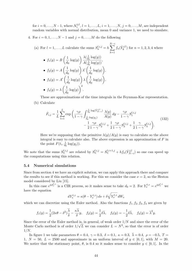
for i = 0, . . . , N−1, where N j,li , l = 1, . . . , L, i = 1, . . . , N, j = 0, . . . ,M , are independent

random variables with normal distribution, mean 0 and variance 1, we need to simulate.

4. For i = 0, 1, . . . , N − 1 and j = 0, . . . ,M do the following

(a) For l = 1, . . . , L calculate the sums Sl,i,jn = hN−i∑k=1

fn(Y j,lk ) for n = 1, 2, 3, 4 where

• f1(y) = B

(1

d0log(y)

)λ( 1

d0log(y))

A( 1d0

log(y)),

• f2(y) = A

(1

d0log(y)

)λ′(

1

d0log(y)

),

• f3(y) = A′(

1

d0log(y)

)λ

(1

d0log(y)

),

• f4(y) = λ

(1

d0log(y)

)2

.

These are approximations of the time integrals in the Feynman-Kac representation.

(b) Calculate

Fi,j =1

L

L∑l=1

exp

(γρ

1− γ

∫ 1d0

log(Y j,lN−i)

1d0

log(yj)

λ(y)

A(y)dy − γρ

1− γSl,i,j1

− 1

2

γρ

1− γSl,i,j2 +

1

2

γρ

1− γSl,i,j3 +

1

2

γ

1− γSl,i,j4

).

(132)

Here we’re supposing that the primitive λ(y)/A(y) is easy to calculate so the aboveintegral is easy to calculate also. The above expression is an approximation of F inthe point F (ti,

1d0

log(yj)).

We note that the sums Sl,i,jn are related by Sl,i,jn = Sl,i+1,jn + hfn(Y j,l

N−i) so one can speed upthe computations using this relation.

5.4 Numerical simulations

Since from section 4 we have an explicit solution, we can apply this approach there and comparethe results to see if this method is working. For this we consider the case ν = 2, so the Hestonmodel considered by Liu [15].

In this case e2Zt,zs is a CIR process, so it makes sense to take d0 = 2. For Y t,z

s = e2Zt,zs we

have the equation

dY t,zs = κ(θ − Y t,z

s ) ds+ δ

√Y t,zs dWs

which we can discretize using the Euler method. Also the functions f1, f2, f3, f4 are given by

f1(y) =1

2(2κθ − δ2)λ

δ− κλ

δy, f2(y) =

1

2δλ, f3(y) = −1

2δλ, f4(y) = λ

2y.

Since the error of the Euler method is, in general, of weak order 1/N and since the error of theMonte Carlo method is of order 1/

√L we can consider L = N2, so that the error is of order

1/N .In figure 1 we take parameters θ = 0.4, γ = 0.3, δ = 0.1, κ = 0.3, λ = 0.4, ρ = −0.5, T =

1, N = 50, L = 2500 and approximate in an uniform interval of y ∈ [0, 1], with M = 20.We notice that the stationary point, θ, is 0.4 so it makes sense to consider y ∈ [0, 1]. In the

44

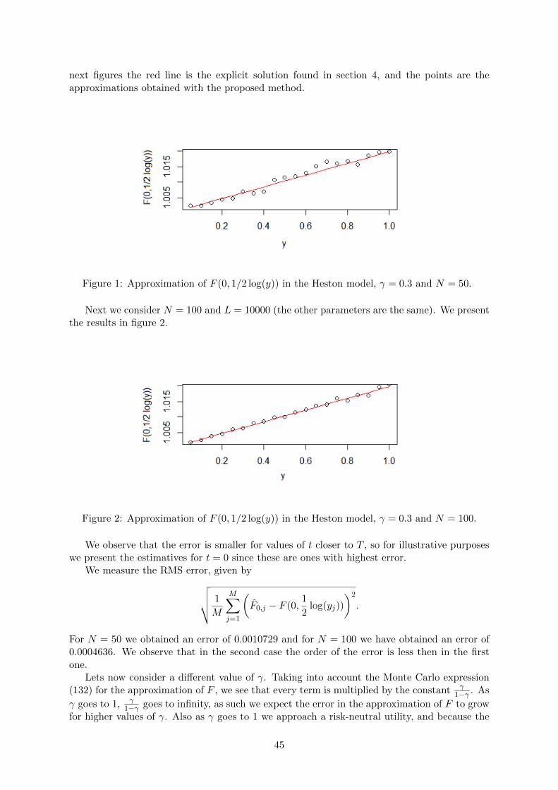
next figures the red line is the explicit solution found in section 4, and the points are theapproximations obtained with the proposed method.

Figure 1: Approximation of F (0, 1/2 log(y)) in the Heston model, γ = 0.3 and N = 50.

Next we consider N = 100 and L = 10000 (the other parameters are the same). We presentthe results in figure 2.


We observe that the error is smaller for values of t closer to T , so for illustrative purposeswe present the estimatives for t = 0 since these are ones with highest error.

We measure the RMS error, given by√√√√ 1

M

M∑j=1

(F0,j − F (0,

1

2log(yj))

)2

.

For N = 50 we obtained an error of 0.0010729 and for N = 100 we have obtained an error of0.0004636. We observe that in the second case the order of the error is less then in the firstone.

Lets now consider a different value of γ. Taking into account the Monte Carlo expression(132) for the approximation of F , we see that every term is multiplied by the constant γ

1−γ . As

γ goes to 1, γ1−γ goes to infinity, as such we expect the error in the approximation of F to grow

for higher values of γ. Also as γ goes to 1 we approach a risk-neutral utility, and because the

45

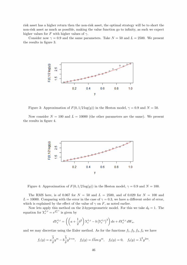
risk asset has a higher return then the non-risk asset, the optimal strategy will be to short thenon-risk asset as much as possible, making the value function go to infinity, as such we expecthigher values for F with higher values of γ.

Consider now γ = 0.9 and the same parameters. Take N = 50 and L = 2500. We presentthe results in figure 3.


Now consider N = 100 and L = 10000 (the other parameters are the same). We presentthe results in figure 4.


The RMS here, is of 0.067 for N = 50 and L = 2500, and of 0.029 for N = 100 andL = 10000. Comparing with the error in the case of γ = 0.3, we have a different order of error,which is explained by the effect of the value of γ on F , as noted earlier.

Now lets apply this method on the 2-hypergeometric model. For this we take d0 = 1. The

equation for Y t,zs = eZ

t,zs is given by

dY t,zs =

((a+

1

2δ2)Y t,zs − b

(Y t,zs

)3)ds+ δY t,z

s dWs,

and we may discretize using the Euler method. As for the functions f1, f2, f3, f4 we have

f1(y) = aλ

δym − bλ

δy2+m, f2(y) = δλmym, f3(y) = 0, f4(y) = λ

2y2m.

46

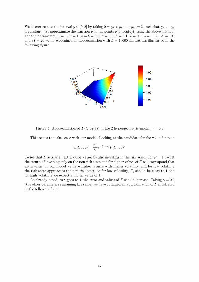
We discretize now the interval y ∈ [0, 2] by taking 0 = y0 < y1, · · · , yM = 2, such that yj+1−yjis constant. We approximate the function F in the points F (ti, log(yj)) using the above method.For the parameters m = 1, T = 1, a = b = 0.3, γ = 0.3, δ = 0.1, λ = 0.3, ρ = −0.5, N = 100and M = 20 we have obtained an approximation with L = 10000 simulations illustrated in thefollowing figure.

Figure 5: Approximation of F (t, log(y)) in the 2-hypergeometric model, γ = 0.3

This seems to make sense with our model. Looking at the candidate for the value function

w(t, x, z) =xγ

γeγr(T−t)F (t, x, z)η

we see that F acts as an extra value we get by also investing in the risk asset. For F = 1 we getthe return of investing only on the non-risk asset and for higher values of F will correspond thatextra value. In our model we have higher returns with higher volatility, and for low volatilitythe risk asset approaches the non-risk asset, so for low volatility, F , should be close to 1 andfor high volatility we expect a higher value of F .

As already noted, as γ goes to 1, the error and values of F should increase. Taking γ = 0.9(the other parameters remaining the same) we have obtained an approximation of F illustratedin the following figure.

47

Figure 6: Approximation of F (t, log(y)) in the 2-hypergeometric model, γ = 0.9

As we can see the maximum value is now 20, while in the previous case it is 1.06, so thevalues of F have increased as predicted. We should also expect a higher order of error for thiscase.

48

6 Concluding Remarks and Future Work

For the portfolio optimization problem, and when considering unbounded utilities, as is the caseof the power utilities, there is no guarantee that the value function will be finite, and there canbe portfolios that generate an infinite payoff, making the problem degenerate and impossibleto solve using the HJB equations. This indeed seems to happen in many cases of stochasticvolatility models. For the model considered in section 4, Korn and Kraft in [12] prove that ifthe condition (85) is not satisfied in the case ν = 2, the problem has portfolios with infinitepayoff. Also if we approach the HJB equations though a Feynman-Kac representation thereare many instances where the expected value seems to be infinite.

Considering some utility function we want to use, one solution could be to transform thisfunction to be constant after some very high value, making it bounded, and so making the valuefunction bounded as well. In a way, since there are high values for the wealth process that canbe nonsensical, having more wealth then that may not have more utility, so this seems like arealistic approach. If one checks our definition of utilities, one sees that we have tried to includethese transformations, by allowing the derivative and second derivative of the utility functionto be 0, where usually in the literature one finds strict inequalities (one needs an interpolationto keep the smoothness of the utility function). In this case, if one can find a bounded functionthat solves the HJB equation, this function satisfies automatically the uniform integrabilitycondition, and so it is the value function.

Another issue with the way we have formulated the portfolio control problem, is that wehave allowed for the portfolio to take any values in R, effectively allowing for unlimited shortsales, which can be unrealistic. Bounding the values that the portfolio can take, one may thenbe able to prove that the value function is finite. Still by doing this, the value function mightnot be smooth, and so we can’t solve the problem through the strategies discussed here. Onthe other hand, it might be possible to solve the problem using viscosity solutions (see [3, 22]).

Numerical methods for general utilities seem to be scarce in the stochastic volatility portfolioproblem, when optimizing utility from terminal wealth. The best one, as far as we know, seemsto be presented in [5], where the authors develop a numerical approximation scheme usingasymptotic methods. Yet, as we have noted, the problem can be not well posed, in the sensethat the value function is infinite, and in this case this approach will not work, so one has tobe careful as to the model one considers. Also the authors only consider the case when theparameters are either large or small (slowly varying and fast varying stochastic volatility) andwe are unsure if this always applies.

In future work we would like to be able to approximate the optimal control. Continuingthe work of section 5.3, and using the same notations, take points 0 = t0 < t1 < · · · < tN = Tand z0 < z1 < · · · < zM and suppose we have an approximation for F in the points (ti, zj), forsome general stochastic volatility model (A,B, µ). Since the function α that determines theoptimal controls is given by

α(t, z) =µ(z)− r

(1− γ)e2z+

ηρA(z)

(1− γ)ez1

F (t, z)

∂F

∂z(t, z),

to approximate the optimal control we need the derivative of F in z. We can use a finitedifference to give an approximation of the derivative of the function F , i.e., if we have adiscretization of points given by z0 < z1 < · · · < zM we can approximate the derivative of Fin the points (ti, zj), i = 0, 1, . . . , N j = 0, . . . ,M − 1, by

∂F

∂z(ti, zj) ≈

F (ti, zj+1)− F (ti, zj)

zj+1 − zj.

where F (ti, zi) correspond to our approximation of F in these points. We can therefore give

49

an estimative for α(ti, zi) by

α(ti, zj) ≈µ(zj)− r

(1− γ)e2zj+

ηρA(zj)

(1− γ)ezj1

F (ti, zj)

F (ti, zj+1)− F (ti, zj)

zj+1 − zj.

Here we have used a forward difference, but we can also use a backward or central difference.However this method may not give a good approximation, due to accumulation of errors andwell known instabilities of finite difference methods.

To overcome these difficulties, we can apply the Malliavin Calculus and write ∂F∂z as an

expectation of a stochastic functional, and then find an approximation using a Monte Carlomethod. This stochastic representation may also be useful to establish the Verification theorem.

50

References

[1] Aıt-Sahalia, Y., & Jacod, J. (2014), High-Frequency Financial Econometrics. PrincetonUniversity Press.

[2] Chacko, G., & Viceira, L. (2005), Dynamic Consumption and Portfolio Choice withStochastic Volatility in Incomplete Markets, The Review of Financial Studies, Volume18, Issue 4, Pages 1369–1402.

[3] Fleming, W., & Soner, H. (2006), Controlled Markov Processes and Viscosity Solutions,Springer.

[4] Fonseca, J., & Martini, C. (2014), The α-Hypergeometric Stochastic Volatility Model,SSRN Electronic Journal.

[5] Fouque, J., & Sircar, R., & Zariphopoulou, T. (2013), Portfolio Optimization & StochasticVolatility Asymptotics. SSRN Electronic Journal. 10.2139/ssrn.2473289.

[6] Friedman, A. (1975), Stochastic differential equations and applications, Volume 1, Aca-demic Press.

[7] Glasserman, P., (2003), Monte Carlo Methods in Financial Engineering, Springer-VerlagNew York.

[8] Heston, S., (1993), A closed-form solution for options with stochastic volatility with ap-plications to bond and currency options. Review of Financial Studies, 6, 327–344.

[9] Karatzas, I., & Shreve, S., (1998), Brownian Motion and Stochastic Calculus, Springer-Verlag New York.

[10] Karatzas, I., & Shreve, S., (1998), Methods of Mathematical Finance, Springer-VerlagNew York.

[11] Klenke, A., (2014), Probability Theory, A Comprehensive Course, Springer-Verlag Lon-don.

[12] Korn, R. & Kraft, H. (2004), On the Stability of Continuous-Time Portfolio Problemswith Stochastic Opportunity Set. Mathematical Finance, Vol. 14, No. 3, pp. 403-414.

[13] Kraft, H. (2005), Optimal portfolios and Heston’s stochastic volatility model: an explicitsolution for power utility, Quantitative Finance, 5:3, 303-313.

[14] Kuo, H. (2006), Introduction to Stochastic Integration, Springer.

[15] Liu, J. (2007), Portfolio Selection in Stochastic Environments. The Review of FinancialStudies, 20(1), 1-39.

[16] R. C. Merton (1969), Lifetime portfolio selection under uncertainty: The continuous-timecase. Review of Economics and statistics, 51:247–257.

[17] R. C. Merton (1971), Optimum consumption and portfolio rules in a continuous-timemodel. Journal of economic theory, 3(4):373–413.

[18] Pham, H. (2007), Optimization methods in portfolio management and option hedging. 3rdcycle. Hanoi (Vietnam), pp.27.

[19] Pham, H. (2009), Continuous-time Stochastic Control and Optimization with FinancialApplications, Springer.

51

[20] Privault, N., & She, Q. (2015) Option pricing and implied volatilities in a 2-hypergeometricstochastic volatility model, Applied Mathematics Letters 53.

[21] Sousa, R., & Cruzeiro, A., & Guerra, M. (2016), Barrier Option Pricing under the 2-Hypergeometric Stochastic Volatility Model, Journal of Computational and Applied Math-ematics.

[22] Touzi, N. (2013), Optimal Stochastic Control, Stochastic Target Problems, and BackwardSDE, Springer.

[23] Zariphopoulou, T. (2001), A solution approach to valuation with unhedgeable risks, Fi-nance and and Stochastics, 5:61.

[24] Zhu, J. (2010), Applications of Fourier Transform to Smile Modeling, Springer.

[25] Zhu, Y., & Avellaneda, M. (1997), A risk-neutral stochastic volatility model, InternationalJournal of Theoretical and Applied Finance, Vol. 1, No. 2, 289–310.

52

Portfolio optimization of stochastic volatility models ...

Documents

Transcript of Portfolio optimization of stochastic volatility models ...