Portfolio Choice and Pricing in Illiquid Markets

Nicolae Garleanu∗

First Version: July 2004This Version: July 4, 2006

Abstract

This paper studies portfolio choice and pricing in markets in which immediatetrading may be impossible, such as the market for private equity and certainover-the-counter markets. Optimal positions are found to depend significantlyand naturally on liquidity: when future liquidity is expected to be higher, agentstake more extreme positions, given that they do not have to hold them for longwhen no longer desirable. Consequently, in markets with more frequent tradinglarger trades should be observed. The price, on the other hand, is not affectedsignificantly by liquidity, due to the mitigating effect of endogenous positionchoice. Extensions with multiple assets and portfolio constraints are consideredamong others.

∗Wharton School, University of Pennsylvania, 3620 Locust Walk, Philadelphia, PA 19104-6367,email garleanu@wharton.upenn.edu. I am grateful for discussions with Domenico Cuoco, DarrellDuffie, Jennifer Huang, Rohit Rahi, Guillaume Rocheteau, Dimitri Vayanos, Pierre-Olivier Weill,and, especially, Lasse Pedersen, as well as for comments from seminar participants at Wharton andthe ASAP conference at the LSE. I am solely responsible for all errors.

1

In many markets completing a trade may require a significant amount time. For in-stance, some investments, such as private equity, are essentially non-tradeable for cer-tain periods. Another example is the over-the-counter (OTC) markets, in which alarge number of assets are traded, including corporate and municipal bonds. Here,the need to locate a suitable counterparty can induce delays, further lengthened whenthe possibility of asymmetric information makes complex due diligence processes nec-essary. Finally, even centralized markets do not operate continuously, in particular inless developed economies.

This paper studies the equilibrium price and optimal portfolio choice in such mar-kets. Given an investor’s inability to change his corporate-bond position quickly, whatprice should he pay for these bonds? How large of a stake in private equity should onetake, given that it cannot be changed for a lengthy period of time?

Using an approximation, I derive closed-form expressions for optimal positions andprice. In particular, I find that the positions depend on the liquidity level in a naturalway: the less easily agents can trade, the less extreme positions they take, in order toavoid being forced into holding for a long time positions that become disadvantageous.For instance, when future trading is expected to be difficult, an institution with currenthigh value for a particular corporate bond — say, due to low correlation with the restof its portfolio — should buy a smaller amount of the bond than it would in a perfectmarket.

The price, on the other hand, depends little on liquidity, due to the effect of endoge-nous portfolio choice. In fact, in the approximation, the price is completely unaffectedby the level of liquidity, contrary to the common intuition that the inability to tradein a timely fashion lowers the price of an asset — equivalently, increases its discountrate. Exact numerical results confirm these findings: positions react strongly to thelevel of liquidity, while the price changes very little with liquidity.

So far, price formation in the presence of illiquidity in the sense of inability to tradeimmediately has been studied in two kinds of models. On one hand, several papers,such as Duffie, Garleanu, and Pedersen (2003) (hereafter, DGP), Weill (2002), andVayanos and Wang (2002), have developed search-based models, in which an agentcan only trade at discrete, random times, usually given by a Poisson process. Inthese models, positions are held to exogenously imposed values, making the derivedprices sensitive to these choices and rendering the study of portfolio choice impossible.1

On the other hand, Longstaff (2005) studies a situation in which one of two assets istraded continuously, while the other is traded only at time 0 and from some time T > 0onwards. This is a stylized framework, but it allows for a meaningful portfolio-choiceproblem. Using numerical methods, Longstaff (2005) finds liquidity impacts on bothasset prices, as well as a significant allocation impact. In Longstaff (2005), gains fromtrade stem from different patience levels, which make one agent keener to sell in order

1Lagos and Rocheteau (2006) is the exception.

2

to finance consumption. In contrast, I analyze agents with hedging needs that changeconsiderably over time — for instance, an underwriter may take on a new issue, a bankmay sell to a client insurance for a particular portfolio, or an agent might change theexposure of her human capital to the risk in certain investments.

The model here works as follows. Time is continuous and infinite. Each of acontinuum of agents is assumed to be able to trade a risky asset only at random timescorresponding to arrivals of a Poisson process, capturing the discontinuous nature oftrading opportunities.2 All agents trading at a given time do so in a Walrasian market— taking the price as given, agents choose asset positions without any restrictions.Agents are risk averse, and the covariances between individual endowments and assetdividends follow Markov processes, generating gains from trade.

I consider an approximation to the model that, in effect, keeps agents risk aversetowards the flow of endowments and asset dividends while making them risk neutraltowards future trading needs and opportunities. Together with the assumptions ondistributions (normality) and preferences (exponential), this leads to marginal utilityflows that are linear in agents’ positions and the correlations between endowments anddividends. Furthermore, the subset of agents accessing the market at any point in timeare representative of all the agents, so that the optimality conditions of trading agentsaggregate into the optimality condition of a (fictional) representative agent holdingthe per-capita supply and having the average endowment-dividend correlation in theeconomy, independently of the liquidity level. This observation yields the equilibriumprice.

Using the price obtained this way, the optimal positions are in turn easily derivedas solutions to linear equations. The positions are impacted naturally by the liquiditylevel. The more liquid the market is going to be in the future, the more any given agentcan deviate currently from the autarchy allocation, since he can subsequently changehis holding more easily if desired, rather than incur the utility cost of a disadvantageousposition. Equivalently, the closer his position can be to the Pareto-optimal allocation.

The portfolio and price results are similar in spirit to those obtaining in exogenoustransaction-cost settings, as studied by Constantinides (1986) or Vayanos (1998), inthat positions are closer to the Pareto-efficient allocation if liquidity is high, while theprice is affected little by liquidity. The mechanism is quite different, though. Withexogenous transaction costs, agents choose to trade less frequently in order to avoidincurring transaction costs, thus allowing holdings to deviate from the perfect-marketoptimum and attenuating the impact of transaction costs on prices.

In this paper, on the other hand, worse liquidity means that an agent’s currentposition has more weight in the determination of her marginal utility, as the positionwill be kept unchanged for a longer period. In particular, if the agent has a large holdingrelative to the per-capita supply, her marginal utility will depend more strongly on this

2Deterministic trading times and trading blackout periods are also modeled, with the same results,in an extension.

3

holding and consequently decrease as liquidity worsens, since the marginal utility flowdecreases in the position. At unchanged prices, therefore, the agent would prefer tochoose a lower position to start with. At the same time, though, high-correlationagents would choose larger positions. The ultimate effect is that markets may clearwith minimal adjustments in prices,3 while the positions move further from the Pareto-optimal levels as liquidity becomes lower.

The position adjustment to liquidity has implications for the volume of trade. Inparticular, the exogenous liquidity level — the ability to trade frequently — has a largereffect on turnover than if the positions were fixed. A testable implication is that, inmarkets where completing trades is (expected to be) faster, the average trade size ishigher (larger blocks are traded). This applies both in situations in which tradingdelays are imposed by the centralized market structure — e.g., overnight closures ormarket operating at low frequencies — and in situations in which centralized marketsare missing and locating a counterparty or performing due diligence is time consuming.

The framework allows for several extensions of interest. For instance, studyingmultiple risky assets reveals an interesting impact of one asset’s liquidity on the holdingsin another asset. Suppose, for example, that one asset is illiquid and a second assetperfectly liquid. It follows, naturally, that a decrease in the first asset’s liquidity results(i) in more extreme positions, and higher volume, in the second asset if the two assetsare substitutes — say, both are used to hedge the same kind of risk, e.g., on-the-run and off-the-run treasuries are used to hedge interest-rate risk — and (ii) in lessextreme positions if the two assets are complements — say, the second asset is usedto hedge risk introduced by the first asset, e.g., corporate bonds are used to hedgeendowment risk and treasuries are used to hedge the interest-rate risk in corporatebonds. Another extension concerns exogenous transaction costs: in this context, itis shown that the ranking of the equilibrium price and the no-transaction-cost one isgiven by the difference between the number of buyers and the number of sellers. Inparticular, in the absence of forced exit, transaction costs decrease the price if andonly if there are more buying than selling agents. Forced exit, on the other hand, hasthe usual price-reduction effect reflecting the amortized future transaction costs, as inAmihud and Mendelson (1986). Naturally, transaction costs have a negative impacton trade volume.

Despite the difference in price-setting mechanism, the results of this model areconsistent with those of previous search-based studies, such as DGP. In particular,binding constraints on portfolio holdings do generate a significant liquidity price effect.This is intuitive, since closing the endogenous adjustment channel leaves only the directeffect of liquidity on the marginal utility of an agent. Thus, with binding short-saleconstraints, for instance, the price increases with the liquidity level, as the marginal

3In the approximation studied there is, of course, no price adjustment, while numerical calculationswith reasonable parameters yield small adjustments. Although these results depend on the CARA-normal assumptions, the intuition for the attenuating effect of the endogenous positions is general.

4

utilities of the low-correlation agents are weighted more and more when setting theprice. This result is entirely compatible with the results of DGP, where the pricealso increases with liquidity if the price is set by the buyers. Furthermore, the resultcomplements such studies as Harrison and Kreps (1978) and Scheinkman and Xiong(2003), showing that over-pricing in the presence of shorting constraints and time-varying agent heterogeneity increases with the level of liquidity, as liquidity enablesagents to trade so as to take advantage of the changing relative valuations of theasset. This is an additional testable implication: controlling for the degree of valuationheterogeneity, higher liquidity should beget more over-pricing.

The paper includes a numerical calibration that illustrates, first of all, that the exactprice effect is, indeed, very small4 (of the order of basis points) for parameters deemedreasonable, while the impact on positions is considerable. In effect, in this model, theability to trade is not important for the price level, but it is an important determinantof agents’ utilities. The liquidity level, therefore, is not immaterial. The example alsoshows that the introduction of short-sale constraints can lead to an important liquidityimpact on the price.

In conclusion, the analysis here suggests that an investor in an illiquid asset suchas private equity should consider her future use for the asset and tilt her positionchoice towards the one that she would prefer in the future, given that subsequentadjustments may be difficult, even impossible. Such assets, however, need not be pricedtoo differently from their liquid counterparts, as long as investors are not constrainedexogenously regarding the positions they can take.

Naturally, the paper is related to the large body of search-based literature, startingwith Diamond (1982). Recently, this literature has been extended to address asset-pricing issues such as liquidity premia in various kinds of markets and marketmaking.5

In particular, this paper complements the analysis in this body of literature by deriv-ing optimal portfolios and the price impact of liquidity without position restrictions,pointing out the extent to which the position restrictions are important for a significantquantitative price impact.

The issue of infrequent adjustment has also received attention recently, with paperssuch as Gabaix and Laibson (2002), Reis (2004), and Chetty and Szeidl (2004) mod-eling agents that adjust their consumption discretely. These papers do not concernthemselves, however, with the determination of asset prices, or the choice of positionsin financial assets. Costly consumption adjustments and portfolio choice, but not assetprices, are studied by Grossman and Laroque (1990).

Beside the infrequent-trading literature, this paper relates to the exogenous trans-action cost literature, which it complements by deriving natural counterparts to theresults found in that kind of environment. (See, for instance, Amihud and Mendelson(1986), Constantinides (1986), Vayanos (1998), and Huang (2003).) It is important,

4The illiquid-market price may be either larger or smaller than the Walrasian one.5See, for instance, Duffie, Garleanu, and Pedersen (2005) for a list of references.

5

however, to note that the friction studied here is conceptually different from exogenoustransaction costs. In particular, exogenous trading delays generate imperfect-tradingutility losses endogenously.

The paper is organized as follows. Section 1 introduces and solves the basic model.Section 2 contains several extensions, treating multiple assets, portfolio constraints,and exogenous transaction costs. Finally, Section 3 concludes and discusses futureresearch avenues, while the Appendix contains proofs and some technical details.

1 Basic Model

This paper considers a two-asset economy.6 One asset is riskless, pays interest at anexogenously given constant rate r, and is available in perfectly elastic supply. Theother assets pays a cumulative dividend with Gaussian increments:

dD(t) = mD dt + σD dB(t), (1)

where mD and σD are constants, and B is a standard Brownian motion with respectto the given probability space and filtration (Ft). The per-capita supply of this assetis Θ, and its price is determined in equilibrium.

There are a continuum of agents, with total mass normalized to 1. Agent i has acumulative endowment process ηi, with

dηi(t) = mη dt + ση dBi(t), (2)

where the standard Brownian motion Bi is defined by

dBi(t) = ρi(t) dB(t) +√

1 − ρi(t)2 dZi(t), (3)

with Zi a standard Brownian motion independent of B and ρi(t) the instantaneouscorrelation between the asset dividend and the endowment of agent i. I assume thatρi, referred to as the type of agent i, follows a Markov process on a finite state spacewith J > 1 points 1 ≥ ρ1 > · · · > ρJ ≥ −1. The transition intensity from state j tostate l is denoted by αjl. The processes B, Zi, and ρi for all i are mutually independent.

Agents have von Neuman-Morgenstern utilities with constant-absolute-risk-aversion(CARA) felicity functions with coefficient γ > 0, and changes in correlation betweendividends and endowment induce them to want to trade. I assume, however, that maybe unable to trade immediately.

There are a couple of real-life situations that can generate this kind of illiquidity.First, in some assets — e.g., private equities — trading is exogenously prohibited fora period of time, while markets for other assets experience periodic closures. Second,

6Section 2.1 considers multiple risky assets.

6

many assets are not traded in centralized markets. Here, in order to trade, an agentmay have to search for a qualified counterparty, or an opportunity to trade. Forinstance, there are many assets, such as given corporate bonds or shares in companiesemerging from Chapter 11, that are only traded by a relatively small number of marketparticipants, who have the required expertise. Finding such a participant that is able totake on a larger position, or willing to sell her stake, takes time. Additional time mightbe required to convince the counterparty that the sale is not motivated by information,too.

I model the infrequent-trading feature by assuming that each agent can trade onlyat a subset of the time line. This subset can be random or deterministic, thus beingable to capture scheduled closures and search difficulties. I describe such a generalformulation at the end of this section, but, for simplicity, I start with the assumptionthat each agent trades at Poisson arrival times. More specifically, each agent comesacross a trading post (or competitive marketmaker), where she takes the price as given,with Poisson intensity λ.

An agent possessing θ shares of the asset has a value function defined as

V (w, ρ, θ) = supc,θ

Et

[

−

∫ ∞

t

e−r(s−t)e−γcs ds∣

∣ ρ(t) = ρ, Wt = w, θ(t) = θ

]

, (4)

s.t.

dWt = (rWt − ct) dt + θ(t) dDt + dηt − Pt dθt, (5)

where W is the agent’s total cash holding at any point in time, c the agent’s con-sumption, and θ the number of shares he owns in the risky asset. The optimizationproblem is further constrained by the requirement that the asset holding be chosenonly at the arrival times of the Poisson process. To avoid Ponzi schemes, I impose thetransversality condition

limT→∞

e−rT Et

[

e−rγWT]

= 0. (6)

Standard calculations (see DGP for details) imply that the value function has theform

V (w, ρ, θ, t) = −e−rγ(w+a+a(θ,ρ,t)), (7)

where

a =1

r

(

log r

γ+ mη −

1

2rγσ2

η

)

(8)

is a constant.The rest of the analysis concentrates on stationary equilibria, so the time argument

will be dropped from all functions.7 Let aj(θ) = a(θ, ρj) be the value-function coeffi-

7Time variation, via fluctuation in λ, αu, or αd can be incorporated in the analysis.

7

cient for an agent with correlation ρj. These coefficients obey the following Hamilton-Jacobi-Bellman equations.

−raj(θ) =∑

l

αjl

e−rγ(al(θ)−aj(θ)) − 1

rγ+ λ sup

θ

e−rγ(−P (θ−θ)+aj(θ)−aj(θ)) − 1

rγ− (9)

κ(θ, ρj),

where

κ(θ, ρ) = θmD −1

2rγ

(

θ2σ2D + 2ρθσDση

)

(10)

is the (mean-variance) instantaneous benefit to the agent from holding position θ whenhaving type ρ.

In a stationary equilibrium, all agents with a given correlation ρj choose the sameposition θj. The positions are determined so that agents maximize their utilities,implying that

P = a′j(θj). (11)

Differentiating (9) with respect to θ, we get

ra′j(θk) =

∑

l

αjle−rγ(al(θk)−aj(θk))(a′

l(θk) − a′j(θk)) + (12)

λe−rγ(−P (θj−θk)+aj(θj)−aj(θk))(P − a′j(θk)) + κ1(θk, ρj),

where κ1 is the partial derivative of κ with respect to its first argument.Equations (9)–(12) cannot be solved in closed form. Consequently, I resort to

an approximation that ignores terms of order higher than 1 in (al(θ) − aj(θ)) . Theaccuracy of this approximation depends on the size of rγ(al(θ) − aj(θ))

2, which canbe shown to be small when r3γ3(ρ1 − ρJ)2σ2

Dσ2η is small. As noted by Vayanos and

Weill (2005), another way to derive the results below is to take the limit as γ → 0while holding γσ2

D and γσ2η constant. In effect, this maintains risk aversion towards

dividend and endowment flows, while inducing risk neutrality towards changes in typeand arrival of trading opportunities. A rigorous statement is made in Theorem 1 below.The numerical example in Section 1.1 demonstrates that the approximation is accuratefor reasonable parameters.

The approximation yields

raj(θ) =∑

l

αjl(al(θ) − aj(θ)) + λ(−P (θj − θ) + aj(θj) − aj(θ)) + κ(θ, ρj) (13)

and

ra′j(θk) =

∑

l

αjl(a′l(θk) − a′

j(θk)) + λ(P − a′j(θk)) + κ1(θk, ρj). (14)

8

Note that the approximate HJB equations (13) obtain exactly when agents arerisk-neutral, but the benefit from holding the asset is quadratic. More precisely, theyobtain when the value functions are given by

aj(θ) = supθ

Et

[

∫ ∞

t

e−r(s−t)κ(

θ(s), ρ(s))

ds −∞∑

s=t

e−r(s−t)Ps∆θ(s)∣

∣ ρ(t) = ρ(0), θ(t) = θ

]

,

where trading is only possible at the arrival times of the individual Poisson process.An immediate consequence is that, in equilibrium, for all k = 1, . . . , J it holds

approximately8 that

P = Et

[∫ ∞

t

e−r(s−t)κ1 (θ(s), ρ(s))∣

∣ θ(t) = θk, ρ(t) = ρk

]

. (15)

Equation (15) is intuitive, stating that the price equals the sum of the stream ofdiscounted marginal utilities from the asset at all future times. (The equation is easilyderived by considering permanent deviations in holdings from the optimal ones.)

An explicit formula for the price follows now from two simple observations. First,by the nature of the choice of trading agents, the agents accessing the market at timet are representative of the population, in the following sense: (i) they hold the averagesupply of the asset at any time s ≥ t, and (ii) the distribution of types among themis the same as in the population at any time s ≥ t. Second, the function κ1 is linear.Consequently, when aggregating Equation (15) over all types trading at t, one gets

P = Et

[∫ ∞

t

e−r(s−t)κ1 (Θ, ρ)

]

(16)

= PW ,

where ρ is the average type in the economy, independent of the trading process. Here,PW is the price that would obtain in the corresponding Walrasian market. Note thatstationarity is not required for this result.

In order to be more explicit, I introduce the following notation. First, let µjk be themass of agents of type j that had type k the last time they traded. Let µk· :=

∑

i µki bethe mass of agents of type ρk. Note that µk· depends only on the transition intensitiesα and not on the trading technology. Also, let µ be defined by

µjk =

(

Et

[∫ τ

t

e−r(s−t) ds

])−1

Et

[∫ τ

t

e−r(s−t)1(ρ(s)=ρj) ds∣

∣ ρ(t) = ρk

]

, (17)

where τ is the first arrival time of a trading opportunity after time t. Thus µjk, forvarious j, give the relative payoff weights of the promises to receive a dollar for any

8Throughout the paper this word will be used to mean up to a term in O(

γ3 [(ρ1 − ρJ )σDση]2)

,

or in the limit sense of Theorem 1.

9

future time s such that ρ(s) = ρj, as long as τ has not occurred by s, given thatρ(t) = ρk. The quantities µ and µ are easily computed using standard Markov-chaincalculations.

Consider an agent of type ρk given the opportunity to trade. The optimality of thechoice θk means that

P = Et

[∫ τ

t

e−r(s−t)κ1(θk, ρ(s)) ds∣

∣ ρ(0) = ρk

]

+ Et

[

e−r(τ−t)]

P, (18)

or

P(

1 − Et

[

e−r(τ−t)])

=

(

Et

[∫ τ

t

e−r(s−t) ds

])

κ1

(

θk,∑

j

µjkρj

)

. (19)

Given the exponential distribution of τ , this implies

P =1

rκ1

(

θk,∑

j

µjkρj

)

. (20)

Note that multiplying this relation by µk· and summing over all k yields (16) again, inthe stationary equilibrium:9

P =1

rκ1 (Θ, ρ) . (21)

Using Equation (20) the optimal quantity choice θk is calculated to be

θk = Θ +ση

σD

(

ρ −∑

j

µjkρj

)

. (22)

The Walrasian holdings can be obtained in the limit as λ → ∞, which gives µjk →

1(j=k), thus implying

θWk = Θ +

ση

σD

(ρ − ρk) . (23)

The expression for the equilibrium holdings is natural. The first term is the per-capita supply. The second reflects the difference in vulnerability to the asset-payoffrisk between the average agent and the agent considered. Thus, if the correlationbetween the agent’s endowment and the asset dividend is going to be relatively high,in expectation, until the next trading opportunity, then the agent will hold a lowerposition, and vice-versa. In particular, if the agent can trade continuously, then it isthe difference between the average correlation and his current correlation that givesthe holding, as can be seen in Equation (23).

The results derived above are collected in the following.

9It is shown in the Appendix that, in a stationary equilibrium,∑

j µj·µkj = µk·.

10

Theorem 1 The economy studied has a stationary equilibrium, determined by equa-tions (9), (11), and (12). The value function and consumption are given by

V (w, ρ, θ) = −e−rγ(w+a+a(ρ,θ))

c(w, ρ, θ) = −log(r)

γ+ r(w + a + a(ρ, θ)).

Furthermore, fix parameters γ, σD, and ση and let σD = σD

√

γ/γ and ση = ση

√

γ/γ.Then, as γ goes to zero, the limit price is

P =µD

r− γ

(

σ2DΘ + ρσDση

)

with ρ =∑

j µjρj, while the limit positions equal

θk = Θ +ση

σD

(

ρ −∑

j

µjkρj

)

.

The liquidity effect on positions is intuitive and easily understood: knowing thatshe may get stuck with an undesirable position for a period of time, an agent willtilt her choice towards the positions desired in the other states in which she is mostlikely to have to keep the position chosen now. In particular, this suggests that agentstake less extreme positions in illiquid markets. Furthermore, it would follow that theaverage trade size is smaller, which reduces volume beyond the direct effect of a worseability to conduct a trade.

Without restrictions on the transition matrix of the correlation process, though, itdoes not follow that less liquidity always results in positions closer to the per-capitasupply. In fact, part (i) of the proposition below states a non-trivial necessary conditionfor such a result. The condition is that the expected correlation conditional on acorrelation change during the next instant, (

∑

j 6=k αkj)−1∑

j 6=k αkjρj, is smaller than

the current correlation if and only if the average correlation is.10 To understand this,consider an agent with a positive expected type change. She consequently takes alower position than she would in a perfectly liquid world, in which only the currenttype would matter. Thus, improved liquidity translates into a higher position.

The following statements hold.11

Proposition 2 (i) For any trading frequency λ < ∞, θW1 < θk < θW

J for all k. Thereexists λ < ∞ such that, for λ > λ, θk is monotonic in λ for all k. Furthermore, θk

10I am indebted to Pierre-Olivier Weill for suggesting first-order approximations in 1/λ. Also, seeLagos and Rocheteau (2006) for a related result.

11From now on, I restrict attention to the approximation, meaning that the precise formulation ofall statements involves letting γ → 0 with σD and ση as in the second part of Theorem.

11

increases strictly in λ for λ > λ if and only if

∑

j 6=k αkjρj∑

j 6=k αkj

> ρk, (24)

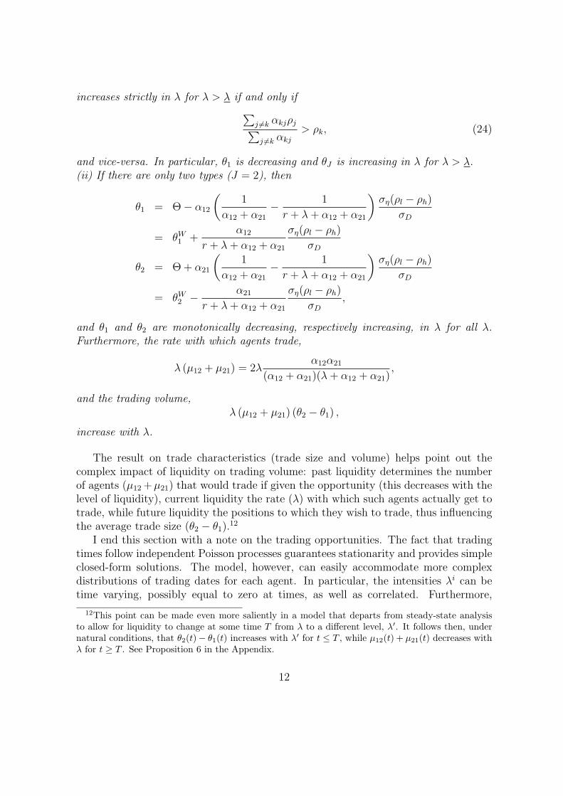
and vice-versa. In particular, θ1 is decreasing and θJ is increasing in λ for λ > λ.(ii) If there are only two types (J = 2), then

θ1 = Θ − α12

(

1

α12 + α21

−1

r + λ + α12 + α21

)

ση(ρl − ρh)

σD

= θW1 +

α12

r + λ + α12 + α21

ση(ρl − ρh)

σD

θ2 = Θ + α21

(

1

α12 + α21

−1

r + λ + α12 + α21

)

ση(ρl − ρh)

σD

= θW2 −

α21

r + λ + α12 + α21

ση(ρl − ρh)

σD

,

and θ1 and θ2 are monotonically decreasing, respectively increasing, in λ for all λ.Furthermore, the rate with which agents trade,

λ (µ12 + µ21) = 2λα12α21

(α12 + α21)(λ + α12 + α21),

and the trading volume,λ (µ12 + µ21) (θ2 − θ1) ,

increase with λ.

The result on trade characteristics (trade size and volume) helps point out thecomplex impact of liquidity on trading volume: past liquidity determines the numberof agents (µ12 +µ21) that would trade if given the opportunity (this decreases with thelevel of liquidity), current liquidity the rate (λ) with which such agents actually get totrade, while future liquidity the positions to which they wish to trade, thus influencingthe average trade size (θ2 − θ1).

12

I end this section with a note on the trading opportunities. The fact that tradingtimes follow independent Poisson processes guarantees stationarity and provides simpleclosed-form solutions. The model, however, can easily accommodate more complexdistributions of trading dates for each agent. In particular, the intensities λi can betime varying, possibly equal to zero at times, as well as correlated. Furthermore,

12This point can be made even more saliently in a model that departs from steady-state analysisto allow for liquidity to change at some time T from λ to a different level, λ′. It follows then, undernatural conditions, that θ2(t)− θ1(t) increases with λ′ for t ≤ T , while µ12(t) + µ21(t) decreases withλ for t ≥ T . See Proposition 6 in the Appendix.

12

α12 α21 γ ρl ρh r mD σD ση Θ10 2 0.8 0.8 0.2 0.1 50 20 20 0.25

Table 1: Parameters used to illustrate price and position impact of variable liquiditylevel. See Section 1.1 for a detailed explanation.

if T o1 ≤ T c

1 < T o2 ≤ T c

2 < · · · is a (possibly infinite) sequence of pairs of stoppingtimes, it can be assumed that all agents (or a random subsample) have continuousaccess to a centralized market between dates T o

i and T ci . As long as an agent’s trading

times are independent of her holding and type, (16) and the appropriate variant of (19)accounting for time dependence in P and µ continue to hold. In particular, the intuitionfor the determination of the position choice is very similar to that in the basic model:knowing that the positions may not be adjustable for a certain period of time, agentsincorporate in their decision their future benefits from ownership. Thus, an agent withhigh present need for the asset takes a smaller position than in a perfect market, giventhat she may be forced to keep the same position even if her need diminished.

1.1 Numerical Example

To illustrate the theoretical results derived so far, I calibrate the model. I consider twotypes of agents and use the parameters in Table 1 to calculate the exact equilibriumprice, as well as the linear approximation to the price for a range of liquidity values(λ). Exact and approximated positions are also calculated.

The parameters are understood as follows: it takes, on average, one tenth of a yearfor an agent’s endowment correlation with the asset to jump back to the low level(ρl = 0.2) from the high level (ρh = 0.8), and half a year for the opposite change.On average, there are Θ = 0.25 shares outstanding per agent. Together with therisk-aversion coefficient γ = 0.8, these parameters result in an equity return premiumaround 5.4%.

Rather than reporting the price, I choose to report the more easily interpretableexcess return on the asset, defined as mD/P − r. Figure 1 shows that the excess returndoes, indeed, vary with liquidity, but that even for low levels of liquidity the impactis very small — for instance, when λ = 10, i.e., wait more than 1 month to trade, thereturn impact is smaller than 4bp. The excess return is noted to decrease with liquiditytowards the Walrasian value, but it can also increase, for different parameters.

Positions, on the other hand, are much more sensitive to liquidity, as can be seenin Figure 2. For instance, if one can trade once a week on average (λ = 52), the lowerposition is about -0.156, which makes it 20% closer to the per-capita supply Θ = 0.25than the Walrasian position, -0.25. The same is true, of course, of the high position.13

13The parameters were chosen to result in short selling in order to illustrate what happens when

13

100

101

102

103

5.42

5.43

5.44

5.45

5.46

5.47

5.48

5.49

5.5

5.51

5.52

Liquidity level (λ)

Exce

ssR

eturn

(%)

Figure 1: Excess-return impact of illiquidity (parameters given by Table 1). Thecontinuous line plots the excess return computed numerically as a function of themeeting intensity λ, while the dashed line indicates the Walrasian excess return.

With less frequent trading, the deviation from the Walrasian positions is even stronger.For instance, with trades every month, on average, the low type is virtually abstainingfrom trading — more precisely, he has a long position of size 0.0005 in the asset.

2 Extensions

The setup is tractable and flexible, and allows for a variety of interesting extensions.First, I consider multiple assets and illustrate the effect of one asset’s liquidity onthe trading in another asset. Second, I show how position constraints make the pricedependent on the level of liquidity. Finally, I add exogenous transactions cost to themodel and discuss their implications on portfolio choice and price.

short sales are not allowed, in Section 2.2.

14

100

101

102

103

−0.3

−0.2

−0.1

0

0.1

0.2

0.3

0.4Exact Approximate

Liquidity level (λ)

Pos

itio

ns

Figure 2: Portfolio sensitivity to illiquidity (parameters given by Table 1). The con-tinuous line plots the exact positions, while the circles show the positions calculatedusing the approximation.

2.1 Multiple Assets

Suppose that the agents can invest in more than one illiquid risky assets, and thattrading times for different assets are independent for any given agent.14 Given theapproximation used, the solution to the allocation problem, once again, is the sameas that in a situation where utility flows are given by the instantaneous mean andvariance of the flow of dividends and endowments. As an implication, however, ifat least two assets are not fully liquid, then the steady-state distribution must haveinfinite support, since agents cannot update positions in these assets simultaneously.Explicit computation of positions, consequently, is quite difficult. That said, it stillholds that the price is not affected by the liquidity level.

An interesting and simpler case is that in which one asset only is illiquid, whilethe other ones are perfectly liquid. For simplicity, let there be only two risky assets,and suppose that asset 2 can be traded continuosly. Here, again, because the holdingof asset 2 is adjusted simultaneously with the holding of asset 1 or with any changein type, there are a finite number of pairs (θ, ρ) in a steady-state equilibrium (J2, in

14If, instead, every agent can trade all assets simultaneously, albeit not continuously — becauseof inertia or inattention, or because all assets are traded in the same market — then the solution isessentially the same as that for one asset, subject to the obvious generalization. Details are omitted.

15

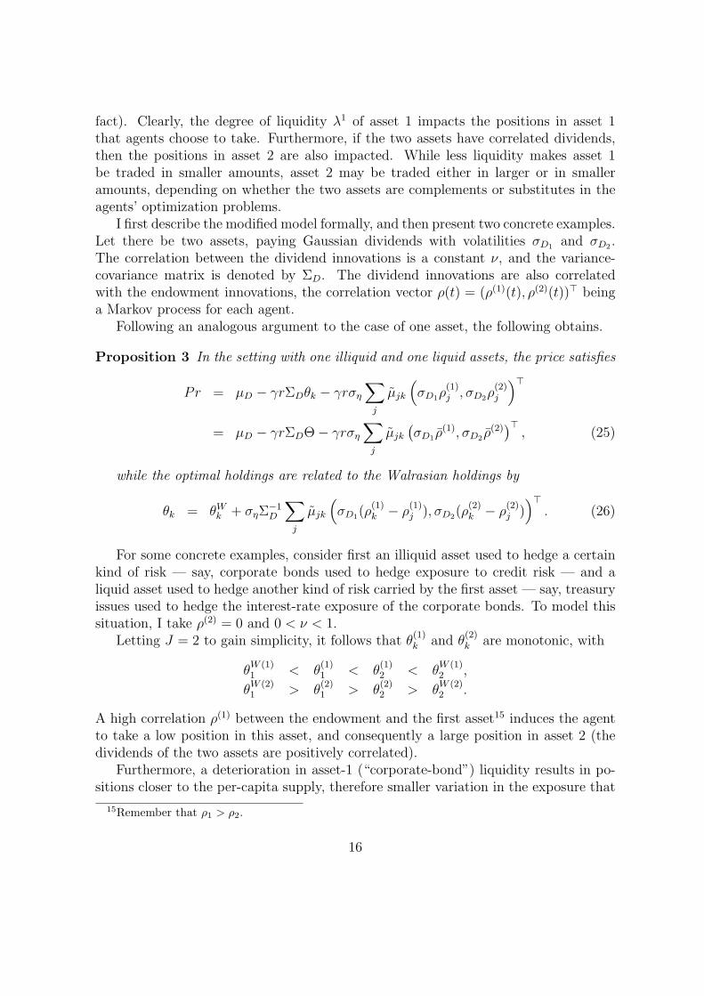
fact). Clearly, the degree of liquidity λ1 of asset 1 impacts the positions in asset 1that agents choose to take. Furthermore, if the two assets have correlated dividends,then the positions in asset 2 are also impacted. While less liquidity makes asset 1be traded in smaller amounts, asset 2 may be traded either in larger or in smalleramounts, depending on whether the two assets are complements or substitutes in theagents’ optimization problems.

I first describe the modified model formally, and then present two concrete examples.Let there be two assets, paying Gaussian dividends with volatilities σD1

and σD2.

The correlation between the dividend innovations is a constant ν, and the variance-covariance matrix is denoted by ΣD. The dividend innovations are also correlatedwith the endowment innovations, the correlation vector ρ(t) = (ρ(1)(t), ρ(2)(t))⊤ beinga Markov process for each agent.

Following an analogous argument to the case of one asset, the following obtains.

Proposition 3 In the setting with one illiquid and one liquid assets, the price satisfies

Pr = µD − γrΣDθk − γrση

∑

j

µjk

(

σD1ρ

(1)j , σD2

ρ(2)j

)⊤

= µD − γrΣDΘ − γrση

∑

j

µjk

(

σD1ρ(1), σD2

ρ(2))⊤

, (25)

while the optimal holdings are related to the Walrasian holdings by

θk = θWk + σηΣ

−1D

∑

j

µjk

(

σD1(ρ

(1)k − ρ

(1)j ), σD2

(ρ(2)k − ρ

(2)j ))⊤

. (26)

For some concrete examples, consider first an illiquid asset used to hedge a certainkind of risk — say, corporate bonds used to hedge exposure to credit risk — and aliquid asset used to hedge another kind of risk carried by the first asset — say, treasuryissues used to hedge the interest-rate exposure of the corporate bonds. To model thissituation, I take ρ(2) = 0 and 0 < ν < 1.

Letting J = 2 to gain simplicity, it follows that θ(1)k and θ

(2)k are monotonic, with

θW (1)1 < θ

(1)1 < θ

(1)2 < θ

W (1)2 ,

θW (2)1 > θ

(2)1 > θ

(2)2 > θ

W (2)2 .

A high correlation ρ(1) between the endowment and the first asset15 induces the agentto take a low position in this asset, and consequently a large position in asset 2 (thedividends of the two assets are positively correlated).

Furthermore, a deterioration in asset-1 (“corporate-bond”) liquidity results in po-sitions closer to the per-capita supply, therefore smaller variation in the exposure that

15Remember that ρ1 > ρ2.

16

can be hedged with asset 2 (“interest-rate exposure”), whence smaller trades in asset2 (“treasuries”).

As a second example, suppose that the liquid and illiquid asset are both used tohedge the same kind of risk — for instance, on-the-run and off-the-run treasuries usedto hedge interest-rate risk. To capture this notion, let ρ(1) = ρ(2) and 0 < ν < 1.

Setting J = 2 once again, it follows that θ(1)k and θ

(2)k are monotonic, but this time

θW (1)1 < θ

(1)1 < θ

(1)2 < θ

W (1)2 ,

θ(2)1 < θ

W (2)1 < θ

W (2)2 < θ

(2)2 .

This time, a high correlation ρ(1) = ρ(2) induces positions in both assets to be low.The interesting feature is that, since a deterioration in the liquidity of asset 1 (the“off-the-run treasuries”) results in less extreme positions in this asset, it also inducesmore variable positions in the second asset (the “on-the-run treasuries”), which is asubstitute.

2.2 Position Constraints

One way to summarize the price implication of the basic model is to say that agentsadjust their investment strategy to the liquidity level, as a result diminishing consid-erably the sensitivity of the price to liquidity. If the position-adjustment channel isshut, on the other hand, intuition suggests that the price should be impacted directlyby changes in liquidity.

Indeed, assume that, at all times, every position θk must satisfy θk ≥ θ.16 Also,let µjk = µk·µjk. For any position θk > θ chosen optimally, the pricing equation (20)holds:

µk·Pr =∑

j

µjkκ1(θk, ρj). (27)

Let us assume that θk > θ if and only if k > k0. Aggregating (27) over the values of kfor which it holds, i.e., k > k0, yields

(

∑

k>k0

µk·

)

Pr =∑

j,k>k0

µjkκ1(θk, ρj),

or

Pr = κ1

(

∑

k>k0

µk·

)−1(∑

k>k0

µk·θk

)

,

(

∑

k>k0

µk·

)−1(∑

j,k>k0

µjkρj

)

.

16It appears meaningful to restrict θ to θ ≤ 0.

17

While lengthy, the expression above is as natural as Equation (21): the price is givenby the per-capita supply of assets held away from the constraints, and the averagediscounted type among unconstrained agents.

Since the amount of the asset held by the constrained agents is independent ofthe liquidity in the market (as long as the same types are constrained), the averageholding of unconstrained agents is constant. Consequently, the price dependence onthe liquidity level is determined by the term

∑

j,k>k0

µjkρj.

Intuition suggests that, as liquidity improves, fewer agents, on average, will be forcedto hold θk when they prefer θj. In other words, µjj goes up, while µjk for j 6= k goesdown with λ. Since ρ decreases in j, this would imply that the average correlationaffecting the price decreases, and thus the price increases.

While intuitive, the argument above is not correct, because the masses µjk neednot be monotonic in λ. In general, though, the following holds.

Proposition 4 Assume that positions are constrained to satisfy θk ≥ θ and considerparameters for which the constraint binds. Then the following holds.

(i) There exists a value λ > 0 such that the price P increases in λ for λ > λ.

(ii) If there are only two types (J = 2), then the price is given by

Pr = κ1(θ2, ρ2) −α21

r + λ + α12 + α21

rγ(ρ1 − ρ2)σDση (28)

and it increases in λ for all λ > 0.

Naturally, the converse of Proposition 4, concerning binding upper limits on posi-tions, is also true. It is debatable, though, whether binding upper limits, due perhapsto agency issues, arise as naturally as lower such as short-sale constraints. Interest-ingly, with more than 2 types, both lower and upper bounds can bind for open sets ofparameters. In that case, the dependence of price on liquidity is parameter specific.

The result of Proposition 4 relates to the findings of Harrison and Kreps (1978) andScheinkman and Xiong (2003). In a setting with shorting constraints and differencesof opinions, they find that the price is increased by the re-sale option of the asset inthe future. Proposition 4 adds the natural refinement that the price increase is higherwhen trading is easier.

It is instructive to extend the numerical example to the case of portfolio constraints.To that end, assume that short sales are not allowed, and compute the price again fora variety of levels of liquidity, given the parameters in Table 1. As can be seen inFigure 2, and is reflected in Figure 3, for low levels of liquidity the optimal holdingsare both positive, so the constraints do not bind and the price is very close to the

18

100

101

102

103

4.7

4.8

4.9

5

5.1

5.2

5.3

5.4

5.5

5.6

5.7

Exact unconstrainedExact constrainedWalrasian unconstrainedApproximate constrained

Liquidity level (λ)

Exce

ssR

eturn

(%)

Figure 3: Excess-return impact of illiquidity in the presence of short-sale constraints(parameters given by Table 1). The continuous line plots the exact unconstrained-holding excess return, the dash-dot line plots the exact constrained-holding excess-return, while the circles graph the approximate constrained-holding excess-return. Thedashed line shows the Walrasian level.

Walrasian price. Beyond a certain threshold, though, the high-correlation agents donot hold any amount of the asset, which fixes the holding of the other agents, too.The excess return decreases as a consequence, to the effect that it becomes about 80bplower than in the illiquid market, as λ goes to infinity. The reason, once again, is theagents’ inability to adjust positions to the level of liquidity.

The numerical example shows that the direct effect of liquidity on the excess returnwhen the positions are constrained can be significant (80bp), and at the same timevirtually canceled by the effect of the endogenous position adjustment.

2.3 Transaction Costs

In addition to the difficulty of accessing the market or finding a counterparty, tradingoften imposes exogenous transaction costs, such as brokerage fees or bid-ask spreads.This subsection extends the model to allow for such a case. In particular, let every agenttrading have to pay transaction costs proportional to the number of shares traded, sothat the unit price paid by the buyer is P + q and the one received by the seller is

19

P − q, for some q ≥ 0. It follows that, for any agent buying at time t,

Pt + q = Et

[∫ ∞

t

e−r(s−t)κ1 (θ(s), ρ(s)) ds∣

∣ θ(t) = θbk, ρ(t) = ρk

]

, (29)

while, for any seller,

Pt − q = Et

[∫ ∞

t

e−r(s−t)κ1 (θ(s), ρ(s)) ds∣

∣ θ(t) = θsk, ρ(t) = ρk

]

. (30)

Note that, for any type ρi there are two positions an agent would trade to, θbi if he

buys and θsi if he sells. Furthermore, an agent of type j holding the optimal position

of an agent of type i 6= j may not trade when given the opportunity, if the transactioncosts are large. If the transaction cost q is small enough, however, such an agent willalways trade if he can. If, in addition, a stationary setting is considered, then agentswhose type is the same as the last time they traded continue to be marginal. That is,Equation (29) holds for all agents of type (θb

i , ρi), while Equations (30) holds for allagents of type (θs

i , ρi). Consequently, one of Equations (29)–(30) holds for any agentaccessing the market at time t.

Let µbij represent the total mass of agents of type ρi who holds θb

j , and define µsij

similarly. Finally, let µb =∑

i,j µbij and µs =

∑

i,j µsij. Aggregating Equations (29)–

(30) over all agents accessing the market at time t, who are representative of the entireeconomy,

P + q(µb − µs) = Et

[∫ ∞

t

e−r(s−t)κ1 (θ(s), ρ(s)) ds

]

= Et

[∫ ∞

t

e−r(s−t)κ1 (Θ, ρ) ds

]

(31)

= PW .

Using Equations (30)–(29), the optimal positions are derived as before. It followsthat

θbk = θk −

q

γσDση

(1 + (µb − µs))

θsk = θk +

q

γσDση

(1 − (µb − µs)),

where θk is the position chosen by both buyers and sellers without transaction costs.Naturally, the buyers’ position is lower than that of the sellers. Furthermore, highertransaction costs induce a buyer to hold more, while a seller to hold less, of the asset.Thus, transaction costs reduce trade volume.

Since the mass of buyers need not equal that of sellers (market clearing means thatthe number of shares bought must equal that of shares sold), the impact of transaction

20

costs on the price may also depend on liquidity. The price effect is negative if, insteady state, there are more buyers than sellers, and otherwise is positive. This featureis intuitive: Given the marginal benefit of holding (an additional unit of) the asset inperpetuity, buyers require price discounts, while sellers price premia, in order to trade.In equilibrium, the positions adjust so that all agents trade, but in order to attractmore buyers than sellers, a price discount is required, and vice-versa.

Note that, in this expression for the price, there is no term capturing the frequencyof trade as in Amihud and Mendelson (1986) and Vayanos (1998). Furthermore, trans-action costs can make an asset price higher. Indeed, the intuition that the requiredreturn is increased by a measure of the amortized future transaction costs relies on thelife-cycle of an agent, who initially buys the asset, then sells it and exits the economy.Over long periods of time, this is a reasonable description of market participants, butarguably less so over shorter periods: institutions, in particular, do not have severelylimited life spans. In this case, the intuition in this paper may be the more relevantone: On one hand, an agent would value the asset less now because of transaction coststo be paid when selling in the future; on the other hand, buying the asset now meansthat the agent will save transaction costs when wanting to buy in the future, resultingin a higher current valuation.

The link with the literature can be made clearer by assuming finite agent life spans.Specifically, suppose that every agent may have to leave the economy with intensityπ. In this case, the agent has immediate access to the market, where he liquidateshis position. The bequeath function is defined as if the agent could only invest in therisk-free asset from then onwards:

V (W ) = −e−rγW . (32)

Consequently, Equations (29)–(30) become

P + q = Et

[∫ τπ

t

e−r(s−t)κ1 (θ(s), ρ(s)) ds∣

∣ buy at t

]

+ (33)

Et

[

e−r(τπ−t)(P − q1(θτπ >0) + q1(θτπ <0))∣

∣ buy at t]

P − q = Et

[∫ τπ

t

e−r(s−t)κ1 (θ(s), ρ(s)) ds∣

∣ sell at t

]

+ (34)

Et

[

e−r(τπ−t)(P − q1(θτπ >0) + q1(θτπ <0))∣

∣ sell at t]

,

where τπ is the arrival time of exit.To preserve stationarity, entry is assumed at the same rate as exit, types being

drawn from the stationary distribution. When aggregating the pricing equations above,only agents choosing their position freely are considered: agents already owning posi-tions and trading to different positions, and agents trading for the first time. Equa-tions (33)–(34) do not hold for agents exiting the economy.

21

Let ιb and ιs be the inflows of buyers and sellers — the ones who, in equilibrium,take a short position — with ιb + ιs = π; λµb and λµs are the flows to the marketof buyers and sellers from the pool of agents already in the economy. AggregatingEquations (33)–(34) yields

Proposition 5 With transaction costs and entry and exit, the steady-state price sat-isfies

P (λ + π) + q(λ(µb − µs) + ιb − ιs) (35)

= (λ + π)Et

[∫ τπ

t

e−r(s−t)κ1 (θ(s), ρ(s)) ds

]

+ (λ + π)Et

[

e−r(τπ−t)P]

+

q(λ + π)Et

[

e−r(τπ−t)(1(θτπ <0) − 1(θτπ >0))]

.

If there is no shorting in equilibrium, the equation above simplifies to

P (λ + π) + q(λ(µb − µs) + π) = (λ + π)

(

r

r + πPW +

π

r + π(P − q)

)

. (36)

As λ → ∞, the price approaches

P = PW −q

r(π + (r + π)(µb − µs)). (37)

Equation (37) captures both price effects that transaction costs have in this setting:πq/r represents the per-share loss q incurred with frequency q, and q(µb −µs)(r +π)/rthe imbalance between losses to buyers and losses to sellers. In particular, even ifµb = µs,17 it holds that P < PW , a conclusion that does not depend on the level λ ofmarket liquidity.

3 Conclusion

This paper studies portfolio choice and pricing in markets in which trading may takeplace with considerable delay. Examples of assets in such a situation include privateequity, which may have to be held without trading for several years, and small corpo-rate and municipal bond issues and shares in firms recently emerged from Chapter 11proceedings, for all of which finding an appropriate buyer or seller may require lengthysearch.

The paper uses an approximation, supported by numerical results, to derive closed-form price and holding expressions. It is found that the liquidity level has a strongimpact on portfolio choice. For instance, when future trading is expected to be difficult,an institution with current high value for a particular corporate bond — say, due to

17This is the case with only two types of investors, for instance.

22

low correlation with the rest of its portfolio — should buy a smaller amount of thebond than it would in a perfect market. The reason is that, as its value for the bonddiminishes, the institution may have to continue maintaining its position for a while.Similarly, if its value from the asset could increase in the future, the institution shouldhold a larger amount if the market is illiquid. A clear empirical implication is thatsmaller blocks should be traded in illiquid markets.

Second, the paper illustrates the dampening effect of endogenous portfolio choiceon the price impact of liquidity. In the context of the approximation studied, thisimpact is actually literally zero, due to a couple of specific assumptions. Generally,the price is affected less by liquidity than the marginal utility of any agent who isheld exogenously to certain positions. An illustration is provided by binding short-sale constraints. These render the endogenous adjustment impossible, and thereforethe price effect of the liquidity level is large. An empirical implication, here, is thatspeculative price bubbles are enhanced by liquidity.

An interesting question not addressed in this paper, and which constitutes the focusof future work, concerns random liquidity correlated with asset fundamentals, perhapsin conjunction with correlated personal liquidity events to individual agents. Thiswould capture the notion of liquidity crunches. The approximation adopted by thispaper would not be the appropriate tool in that case.

23

A Appendix

Mass Distribution in Steady State

First of all, note that, under the standing assumptions, in equilibrium there are a totalof J2 kinds of agents, where each kind is identified by the tuple σ = (ρ, θ). Note that,in steady state, the mass of (ρj, θk)-agents is µjk. Since the masses are constant, thenet outflow from type (ρj, θk) — in short, type jk — is 0:

0 = −µjk

∑

l 6=j

αjl +∑

l 6=j

αljµlk − 1(j 6=k)λµjk + 1(j=k)λ∑

l 6=j

µjl

= −µjk

∑

l 6=j

αjl +∑

l 6=j

αljµlk − λµjk + 1(j=k)λ∑

l

µjl. (A.1)

The expressions in the first row above have a straightforward justification. (The secondrow is just a manipulation of the first.) The first term represents the rate at whichagents of kind jk change their kind because the correlation coefficient changes. Thesecond term represents the rate at which agents of other types holding θk become ofkind jk as a result of a type change. The third and fourth terms record the results ofchanges due to trading: if an agent of kind jk does not have the optimal position, thatis, j 6= k, then upon trading he changes kind, leaving the pool jk. If j = k, then allother kinds lk trade to become of kind jk, joining the pool.

Note that summing over Equation (A.1) above over j gives

∑

j

µjk =∑

j

µkj, (A.2)

meaning that the total mass of agents holding θk shares is the same as the total massof type k.

Finally, it holds that18∑

j

µkj =∑

j

µjk = µk·.

Proof of Theorem 1:

The theorem is proved almost entirely in the main body of the text. Existence ofthe equilibrium and the form of the value functions and optimal consumption followalong the same lines of reasoning as in DGP, and are consequently omitted. Theapproximations follow immediately from the fact that the equilibrium value-functioncoefficients aj(θk) and price are bounded as γ → 0 keeping γσDση fixed.

�

18In fact, µjk are the steady-state masses corresponding to a trading intensity λ = λ + r.

24

Proof of Proposition 2:

For part (i), note from Equations (22) and (23) that

θk = θWl −

ση

σD

(

∑

j

µjkρj − ρl

)

. (A.3)

Since ρ1 and ρJ are the maximum, respectively minimum, values that ρ can take,θW1 < θk < θW

J .Furthermore, the quantities µjk are rational functions of λ, and consequently so are

θk. Therefore, the quantities θk have only a finite number of local maxima or minima.Consider λ higher than all such local extremes.

Up to terms in O(λ−2) for large λ, it is easily seen that, with j 6= k,

µkk ≃ 1 −

∑

i6=k αki

λ(A.4)

µjk ≃αkj

λ, (A.5)

and, consequently,

θk ≃ θWk −

1

λ

ση

σD

∑

j 6=k

αkj(ρj − ρk). (A.6)

Since θk is monotonic in λ, the sign of its dependence is given by that of∑

j 6=k αkj(ρj −

ρk). It is clear that θ1 decreases, while θJ increases with λ for λ > λ.For part (ii) one calculates explicitly the quantities

µkk =r + λ + αk

r + λ + α1 + α2

(A.7)

µ1· =α21

α12 + α21

(A.8)

µ12 =α12α21

(α12 + α21)(λ + α12 + α21)(A.9)

µ21 = µ12. (A.10)

�

Proposition 6 Consider a market with two types (J = 2), and fix a certain distribu-tion of holdings at time 0, with the types distributed as in steady state. Let the meetingintensity be given by λ(t) = λ for t < T and λ(t) = λ′ for t ≥ T . Then

(i) θ1(t) decreases and θ2(t) increases with λ′ for all t ≤ T ;

25

(ii) µ12(t) + µ21(t) decreases with λ for t > T , provided that T > T for some Tdepending on the initial distribution µ;

(iii) µ12(t) + µ21(t) decreases with λ for all t, provided that µ12 ≥ µ∗12 and µ21 ≥ µ∗

21,where µ∗

jk is the steady-state value of µjk corresponding to λ.

The conditions ...Proof of Proposition 6:

For part (i), start from

Et

[∫ τ

t

e−r(s−t)κ1(θk(t), ρ(s)) ds∣

∣ ρ(t) = ρk

]

= Et

[∫ τ

t

e−r(s−t)κ1(Θ, ρ) ds

]

.

Using the linearity of κ1, it follows that

θk(t) = Θ +

(

ρk −Et

[∫ τ

te−r(s−t)ρ(s)

∣

∣ ρ(t) = ρk

]

Et

[∫ τ

te−r(s−t)

]

)

ση

σD

= Θ +

(

ρk −

∫ ∞

t

Ψ (s; λ, λ′) Et

[

ρ(s)∣

∣ ρ(t) = ρk

]

ds

)

ση

σD

,

where Ψ is defined by the last equation, and is the only quantity that depends on λ′.To finish the proof, note that

∫ ∞

t

Ψ (s; λ, λ′) ds = 1,

that ∂Ψ∂λ′

> 0 if and only if s > s for some s > T , and that Et

[

ρ(s)∣

∣ ρ(t) = ρk

]

ismonotonic in s.

For parts (ii) and (iii), let µ = (µ12, µ21)⊤. For t ≤ T ,

µ(t) = µ∗ + e−At (µ(0) − µ∗) , (A.11)

where

A =

[

λ + α12 α21

α12 λ + α21

]

and µ∗ is the steady-state value of µ corresponding to λ.�

26

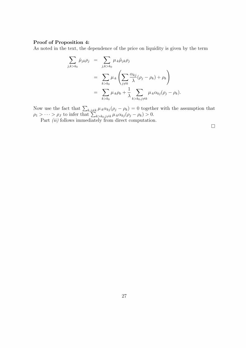
Proof of Proposition 4:

As noted in the text, the dependence of the price on liquidity is given by the term

∑

j,k>k0

µjkρj =∑

j,k>k0

µ·kµjkρj

=∑

k>k0

µ·k

(

∑

j 6=k

αkj

λ(ρj − ρk) + ρk

)

=∑

k>k0

µ·kρk +1

λ

∑

k>k0,j 6=k

µ·kαkj(ρj − ρk).

Now use the fact that∑

k,j 6=k µ·kαkj(ρj − ρk) = 0 together with the assumption thatρ1 > · · · > ρJ to infer that

∑

k>k0,j 6=k µ·kαkj(ρj − ρk) > 0.Part (ii) follows immediately from direct computation.

�

27

References

Amihud, Y. and H. Mendelson (1986). Asset Pricing and the Bid-Ask Spread. Journalof Financial Economics 17, 223–249.

Chetty, R. and A. Szeidl (2004). Consumption Commitments: Neoclassical Founda-tions for Habit Formation. Working Paper, University of Califorina, Berkeley.

Constantinides, G. M. (1986). Capital Market Equilibrium with Transaction Costs.Journal of Political Economy 94, 842–862.

Diamond, P. (1982). Aggregate Demand Management in Search Equilibrium. Journalof Political Economy 90, 881–894.

Duffie, D., N. Garleanu, and L. H. Pedersen (2003). Valuation in Over-the-CounterMarkets. Graduate School of Business, Stanford University.

Duffie, D., N. Garleanu, and L. H. Pedersen (2005). Over-the-Counter Markets.Econometrica 73, 1815–1847.

Gabaix, X. and D. Laibson (2002). The 6D Bias and the Equity Premium Puzzle. InB. Bernanke and K. Rogoff (Eds.), NBER Macroeconomics Annual, Volume 16,pp. 257–312.

Grossman, S. J. and G. Laroque (1990). Asset Pricing and Optimal Portfolio Choicein the Presence of Illiquid Durable Consumption Goods. Econometrica 58, 25–51.

Harrison, J. M. and D. M. Kreps (1978). Speculative Investor Behavior in a StockMarket with Heterogeneous Expectations. Quarterly Journal of Economics 92,323–336.

Huang, J. and J. Wang (2005). Market Liquidity and Asset Prices under CostlyParticipation. Working paper, University of Texas at Austin.

Huang, M. (2003). Liquidity Shocks and Equilibrium Liquidity Premia. Journal ofEconomic Theory 109, 104–129.

Lagos, R. and G. Rocheteau (2006). Search in Asset Markets. Working paper, NYU.

Longstaff, F. (2005). Financial Claustrophobia: Asset Pricing in Illiquid Markets.Working paper. UCLA.

Reis, R. (2004). Inattentive Consumers. Working Paper, Princeton University.

Scheinkman, J. and W. Xiong (2003). Overconfidence, Short-Sale Constraints, andBubbles.

Vayanos, D. (1998). Transaction Costs and Asset Prices: A Dynamic EquilibriumModel. Review of Financial Studies 11, 1–58.

28

Vayanos, D. and T. Wang (2002). Search and Endogenous Concentration of Liquidityin Asset Markets. Working Paper, MIT.

Vayanos, D. and P.-O. Weill (2005). A Search-Based Theory of The On-The-RunPhenomenon. Working Paper, London School of Economics.

Weill, P.-O. (2002). The Liquidity Premium in a Dynamic Bargaining Market. Work-ing Paper, Stanford University.

29