Poro Elastic

GEOPHYSICS, VOL. 62, NO. 6 (NOVEMBER-DECEMBER 1997); P. 1867–1878, 10 FIGS., 2 TABLES.

Poroelastic Backus averaging for anisotropiclayered fluid- and gas-saturated sediments

Stephan Gelinsky∗ and Sergei A. Shapiro‡

ABSTRACT

A homogeneous anisotropic effective-medium modelfor saturated thinly layered sediments is introduced. Itis obtained by averaging over many layers with differentporoelastic moduli and different saturating fluids. For amedium consisting of a stack of vertically fractured hori-zontal layers, this effective medium is orthorhombic. Wederive the poroelastic constants that define such mediain the long-wavelength limit as well as the effective large-scale permeability tensor. The permeability shows stronganisotropy for large porosity fluctuations.

We observe pronounced effects that do not exist inpurely elastic media. At very low frequencies, seismicwaves cause interlayer flow of pore fluid across inter-faces from more compliant into stiffer layers. For higherfrequencies, the layers behave as if they are sealed, and

no fluid flow occurs. The effective-medium velocitiesof the quasi-compressional waves are higher in the no-flow than in the quasi-static limit. Both are lower thanthe high-frequency, i.e., ray-theory limit. Partial satura-tion affects the anisotropy of wave propagation. In theno-flow limit, gas that is accumulated primarily in thestiffer layers reduces the seismic anisotropy; gas that istrapped mainly in layers with a more compliant frametends to increase the anisotropy. In the quasi-static limit,local flow keeps the anisotropy constant independentof partial saturation effects. For dry rock, no-flow andquasi-static velocities are the same, and the anisotropycaused by layering is controlled only by fluctuations ofthe layer shear moduli. If the shear stiffness of all lay-ers is the same and only the compressive stiffness orsaturation varies, only the ray-theory velocity exhibitsanisotropy.

INTRODUCTION

Both reservoir rocks and their overburden often consist ofthinly layerd sediments. These thin layers can be detected andinvestigated by ultrasonic core measurements, with sonic logs,and by means of other borehole geophysical methods (Dewan,1983; Sams, 1995). Properties of single layers, such as perme-ability and fluid saturation, that are important to delineate apay zone thus can be determined. If more global informationabout the reservoir’s extension, fluid content, and continuityis needed, seismic waves with longer wavelengths are applied.The wavelength ranges from (approximately) millimeters forultrasonics to centimeters for sonic logs and up to many metersfor vertical seismic profiles (VSP) (1–10 m) and surface seis-mic investigations (10–100 m). With a wavelength much longerthan the layer thicknesses, a single layer cannot be resolved.However, fluctuations of the poroelastic constants, of the den-sity, and of the fluid saturation from layer to layer and their

Manuscript received by the Editor April 29, 1996; revised manuscript received January 2, 1997.∗Formerly Geophysical Institute, Karlsruhe University, Hertzstrasse 16, D-76187 Karlsruhe, Germany; presently Western Atlas Logging Services,10201 Westheimer, Houston, Texas 77042. E-mail: [email protected].‡Geophysical Institute, Karlsruhe University, Hertzstrasse 16, D-76187 Karlsruhe, Germany. E-mail: [email protected]© 1997 Society of Exploration Geophysicists. All rights reserved.

correlations affect the seismic wavefield and thus the recordedsignal.

Wave propagation in fluid-saturated media is commonly de-scribed by the Biot theory (Biot, 1956a, 1956b, 1962; Frenkel,1944). This theory predicts frequency-dependent velocities fortwo kinds of compressional waves and for shear waves inporous, fluid-saturated rock. The displacements of the solidand fluid phases are coupled. Dissipation is caused by theglobal flow, which is the relative motion of both continuousphases. Biot theory is an effective-medium theory in the sensethat it replaces a medium that is microscopically inhomoge-neous (porous) with a homogeneous effective medium. Theeffective Biot parameters can be derived exactly from the mi-crostructure. An overview is given in Bourbie et al. (1987).To model heterogeneous, layered, saturated porous rock, weapply Biot theory in two ways. First, we describe each homo-geneous layer by Biot theory. Second, we parameterize thehomogeneous, anisotropic effective medium that replaces the

1867

Downloaded 06 May 2009 to 140.105.64.32. Redistribution subject to SEG license or copyright; see Terms of Use at http://segdl.org/

1868 Gelinsky and Shapiro

stack of layers in the long-wavelength limit in terms of Biottheory.

Heterogeneous, poroelastic media are characterized by sev-eral critical frequencies, all separating low- and high-frequencyregimes with respect to different physical mechanisms. Upscal-ing means transforming results that were measured or modeledin one frequency range to a lower one. For example, seismicvelocities measured at core samples can be upscaled to predictsonic log velocities. The first basic scale is defined by the ratiobetween the wavelength λ of an incident wave and a typicallength d that describes medium heterogeneities. This d may bethe average layer thickness, half a period in periodically layeredmedia, or the correlation length of random heterogeneities. If

d

λ¿ 1, (1)

the system is well described by effective-medium theories. Inthe opposite limit, for λ

d ¿ 1, the wave propagates alonga straight ray in each homogeneous layer, and the completeraypath is defined by Fermat’s principle. This limiting caseis addressed as ray theory throughout this paper. There is alarge zone of intermediate values of λ/d at which a transi-tion from effective-medium to ray-theory behavior can be ob-served if the layer thicknesses increase from some centimetersto many meters or if the seismic wavelength decreases (Marionet al., 1994; Tang and Burns, 1992). In this range, the frequencydependence of seismic wavefield parameters becomes impor-tant. Applying the generalized O’Doherty-Anstey formalismfor elastic waves, Shapiro and Hubral (1996) found that theanisotropy of the phase velocity even at seismic frequencies canbe significantly below the one derived in the static limit (i.e.,the Backus averaging for anisotropy). Using surface seismicand borehole information, one can take thin layering into ac-count directly and correct the amplitude-variation-with-offsetresponse of a target zone with a thinly layered elastic overbur-den for effects caused by the stack of layers (Widmaier et al.,1995, 1996).

The response of poroelastic, fluid-saturated media to seis-mic excitations is a complicated function of frequency evenin the absence of any large-scale heterogeneities. In the quasi-static limit, i.e., for frequencies below a characteristic frequency

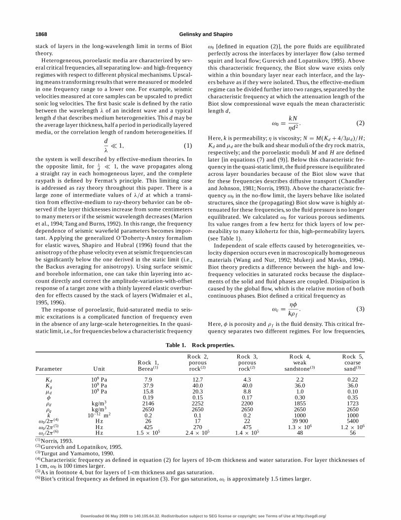
Table 1. Rock properties.

Rock 2, Rock 3, Rock 4, Rock 5,Rock 1, porous porous weak coarse

Parameter Unit Berea(1) rock(2) rock(2) sandstone(3) sand(3)

Kd 109 Pa 7.9 12.7 4.3 2.2 0.22Kg 109 Pa 37.9 40.0 40.0 36.0 36.0µd 109 Pa 15.8 20.3 8.8 1.0 0.10φ 0.19 0.15 0.17 0.30 0.35ρd kg/m3 2146 2252 2200 1855 1723ρg kg/m3 2650 2650 2650 2650 2650k 10−12 m2 0.2 0.1 0.2 1000 1000

ω0/2π (4) Hz 26 17 22 39 900 5400ω0/2π (5) Hz 425 270 475 1.3 × 106 1.2 × 106

ωc/2π (6) Hz 1.5 × 105 2.4 × 105 1.4 × 105 48 56(1)Norris, 1993.(2)Gurevich and Lopatnikov, 1995.(3)Turgut and Yamamoto, 1990.(4)Characteristic frequency as defined in equation (2) for layers of 10-cm thickness and water saturation. For layer thicknesses of1 cm, ω0 is 100 times larger.(5)As in footnote 4, but for layers of 1-cm thickness and gas saturation.(6)Biot’s critical frequency as defined in equation (3). For gas saturation, ωc is approximately 1.5 times larger.

ω0 [defined in equation (2)], the pore fluids are equilibratedperfectly across the interfaces by interlayer flow (also termedsquirt and local flow; Gurevich and Lopatnikov, 1995). Abovethis characteristic frequency, the Biot slow wave exists onlywithin a thin boundary layer near each interface, and the lay-ers behave as if they were isolated. Thus, the effective-mediumregime can be divided further into two ranges, separated by thecharacteristic frequency at which the attenuation length of theBiot slow compressional wave equals the mean characteristiclength d,

ω0 = kN

ηd2. (2)

Here, k is permeability; η is viscosity; N = M(Kd + 4/3µd)/H ;Kd andµd are the bulk and shear moduli of the dry rock matrix,respectively; and the poroelastic moduli M and H are definedlater [in equations (7) and (9)]. Below this characteristic fre-quency in the quasi-static limit, the fluid pressure is equilibratedacross layer boundaries because of the Biot slow wave thatfor these frequencies describes diffusive transport (Chandlerand Johnson, 1981; Norris, 1993). Above the characteristic fre-quency ω0 in the no-flow limit, the layers behave like isolatedstructures, since the (propagating) Biot slow wave is highly at-tenuated for these frequencies, so the fluid pressure is no longerequilibrated. We calculated ω0 for various porous sediments.Its value ranges from a few hertz for thick layers of low per-meability to many kilohertz for thin, high-permeability layers.(see Table 1).

Independent of scale effects caused by heterogeneities, ve-locity dispersion occurs even in macroscopically homogeneousmaterials (Wang and Nur, 1992; Mukerji and Mavko, 1994).Biot theory predicts a difference between the high- and low-frequency velocities in saturated rocks because the displace-ments of the solid and fluid phases are coupled. Dissipation iscaused by the global flow, which is the relative motion of bothcontinuous phases. Biot defined a critical frequency as

ωc = ηφ

kρ f. (3)

Here, φ is porosity and ρ f is the fluid density. This critical fre-quency separates two different regimes. For low frequencies,


Poroelastic Backus Averaging 1869

the fluid motion is dominated by viscosity, whereas for fre-quencies above ωc, inertia and tortuosity are more important(Rasolofosaon, 1991). For the materials that we have studiedin more detail, we give ωc in Table 1. For frequencies belowωc, the velocity can be calculated according to Gassmann’s for-mula (White, 1983). For high frequencies, as in the ray-theorylimit, the velocity is slightly higher. Geertsma and Smit (1961)derived a simple expression for the Biot high-frequency lim-iting P-wave velocity [equation (16)], which we discuss in thesection on no-flow limit.

In this paper, we transform Biot’s second-order differen-tial equations to a system of first-order differential equations.By averaging over all layers, the heterogeneous medium is re-placed by a homogeneous effective medium. Fluctuations ofthe poroelastic constants from layer to layer lead to anisotropy.In the low-frequency limit, the layered medium behaves likean anisotropic homogeneous effective medium with the z-axisas a symmetry axis. This averaging is a generalization of theBackus averaging technique, originally proposed for elasticmedia (Backus, 1962; Bruggemann, 1937).

For isotropic layers, the results for the poroelastic moduliare consistent with those given in Norris (1993). Additionally,with the new method, the complete poroelastic tensor is de-termined and upscaling rules for the permeability tensor areautomatically included. Thus, this technique can serve as a basisto study the influence of porosity fluctuations and fluid proper-ties on the propagation of obliquely incident q P, qS1, and qS2

seismic plane waves in a poroelastic, fluid-saturated, fractured,finely layered medium, taking thin layering consistently intoaccount. Such a numerical modeling of wave propagation forporoelastic media with anisotropy caused by an anisotropic dryframe was presented recently in Carcione (1995).

After the introduction of the poroelastic generalization ofBackus averaging, basic results for isotropic layers are derivedand compared for various limiting cases (quasistatic, no flow,and ray theory). The influence of partial saturation is discussedfor different media (see Figures 2 to 8). Next, the scheme is gen-eralized to anisotropic layers (e.g., layers containing shale oraligned fractures). Finally, the behavior of the effective perme-ability is considered, and permeability anisotropy as a function

FIG. 1. Vertically fractured and horizontally layered medium.The single layers are TIH, with the x-axis as the symmetry axis.The effective medium is orthorhombic.

of porosity fluctuations is investigated (see Figures 9 and 10).The paper concludes with a discussion of the results.

THEORY

Dynamic equations

Starting points are the second-order Biot (1962) differentialequations

∂

∂xjτi j = ∂2

∂t2(ρui + ρ fwi ) (4)

and

− ∂

∂xip f = ∂2

∂t2(ρ f ui + qi jw j ). (5)

On the left-hand sides, τi j and pf are the elements of the stresstensor and the hydrostatic pressure. For isotropic layers, thestress-strain relations are given later [in equation (10)]. Thevariables u and w are the displacement of the solid phase andthe relative solid-fluid displacement, respectively; the indices i ,j denote the Cartesian coordinates; and ρ = φρ f + (1−φ)ρg isthe density of the saturated composite. Throughout this paper,the index d is used for properties of the dry rock frame, i.e., thematrix; the index g is used for properties related to the grain,i.e., the matrix material; and the index f is used for fluid prop-erteis. The permeability enters into the Biot equations throughthe dissipation term qi j . Permeability and tortuosity are ten-sors with elements ki j and ai j , respectively. With

˜r =

˜k−1, the

definition of qi j is

qi j = iηri j

ω+ ρ f ai j

φ. (6)

In the isotropic case, qi j =qδi j , since permeability ki j = kδi j andtortuosity ai j =aδi j . A closer look at the frequency dependenceof q explains the definition of Biot’s characteristic frequencyωc as given by equation (3). The tortuosity that is numericallyclose to unity usually is omitted.

Following Biot, we parameterize each layer by its poros-ity, permeability, density, several poroelastic constants, and thefluid parameters viscosity, density, and bulk modulus. The tor-tuosity becomes important only above Biot’s critical frequency.The necessary number of parameters depends on the symme-try properties of the layer materials. Isotropic layers are spec-ified by four poroelastic constants and one value of perme-ability; transversely isotropic (TI) layers are specified by eightporoelastic constants and two values of directional permeabil-ity. The specification of poroelastic media requires more con-stants than does that of elastic media. These are needed becauseof the existence of an additional fluid phase and its influence onthe compressibility of the saturated rock. Biot and Willis (1957)discuss the measurements that are needed to determine all Biotconstants by means of jacketed and unjacketed compressibilitytests in the laboratory. The number of additional parametersdepends on the symmetry of the medium. For isotropic media,the two constants are σ and M ,

σ = 1− Kd

Kg,

M =[φ

K f+ σ − φ

Kg

]−1

. (7)

Here, Kg is the grain bulk modulus (the material of the dryframe) and K f is the fluid bulk modulus. For TI media, three



additional parameters are required (B6, B7, B8 or P, Q, R);for orthorhombic media, four are required (M1, M2, M3, M).The maximum number of additional poroelastic constants inthe most general case of anisotropy is seven; i.e., the mediumis characterized by 28 constants.

We study plane-wave propagation in vertically inhomoge-neous media. Therefore, we use the following starting pointfor the displacement of the solid phase u (and, respectively, forthe relative solid-fluid displacement w and the stresses τi j ):

u = (ux(z),uy(z),uz(z))e−iωt+i pxx+i pyy. (8)

The hydrostatic pressure pf is treated in a similar way. Forisotropic P- and SV-wave problems and those with transverseisotropy and a vertical symmetry axis (TIV), the descriptioncan be simplified by setting py, uy, andwy equal to zero withouta loss of generality. To develop the basic concepts, we first dis-cuss isotropic layers and use this simplification. Later, we dis-cuss the more general case of non-TIV anisotropic layers. Thesaturated P-wave modulus is defined, according to Gassmann,as

H = Kd + 43µd + σ 2 M. (9)

The (nonzero) stress-strain relations are (the prime denotingthe derivative with respect to z)

τxx = H∇u− 2µu′z+ σM∇w,

τyy = H∇u− 2µ∇u+ σM∇w,

τzz= H∇u− 2µi pxux + σM∇w, (10)

τzx = µ(i pxuz+ u′x),

−pf = σM∇u+ M∇w.

According to our starting point, ∇u = i pxux + u′z and ∇w =i pxwx +w′z. Furthermore, we transform the second-order Biotdifferential equations to a system of first-order differentialequations, as is common in the elastic case (see, e.g., Aki andRichards, 1980). The medium is now characterized by

dζ

dz+

˜Pζ = 0. (11)

Here, ζ = (ux,uz, wz, τxz, τzz, pf )T and˜P is a (6 × 6) matrix,

consisting of combinations of the above-defined layer parame-ters and describing the P- and SV-wave propagation. The exactexpressions for

˜P and for the equation that describes SH-waves

are given in the Appendix.

TI effective medium

Next, we consider instead of the single layer the whole stackof layers in the long-wavelength (i.e., effective-medium) limit.As we did for each single layer, we can write the Biot equa-tions for a homogeneous, anisotropic medium that will be iden-tified as the effective medium, replacing the layered one afteraveraging. For isotropic layers and for TIV layers (which aretransversely isotropic and have a vertical symmetry axis as thestack of layers), this medium is determined by eight poroelasticconstants B∗1 , B∗2 , . . ., B∗8 and two effective directional perme-abilities k∗z and k∗xy. B∗1 , B∗2 , . . ., B∗8 are defined according to Biot(1962), and the TIV stress-strain relations are

τxx = i px(2B∗1 + B∗2

)ux + B∗3 u′z− B∗6∇w,

τyy = i px B∗2 ux + B∗3 u′z− B∗6∇w,

τzz= i px B∗3 ux + B∗4 u′z− B∗7∇w, (12)

τzx = B∗5 (i pxuz+ u′x),

−pf = i px B∗6 ux + B∗7 u′z− B∗8∇w.

With starting point similar to that of equation (8), a matrix

˜P∗ is determined.

˜P∗ characterizes the anisotropic effective

medium with respect to the q P- and qSV-wave propagationand is defined in the Appendix together with the SH-waveequation. Since we are interested in solutions in the zero fre-quency limit, we can use the condition ζ∗ = 〈ζ〉. We identifythe above-defined TI medium as the effective medium thatreplaces the heterogeneous medium after averaging, so that

˜P∗ = 〈

˜P〉. (13)

ISOTROPIC LAYERS

We compare both matrices element by element by keepingonly the terms of lowest order in frequency. In this way, wefind the effective poroelastic constants and simple relationsfor the densities ρ∗ = 〈ρ〉 and ρ∗f = 〈ρ f 〉. The results for thepermeability in q∗xy and q∗z are discussed below.

Effective medium: Quasi-static limit

The quasi-static effective poroelastic constants are

B∗1 = 〈µd〉,

B∗2 = 2⟨

λdµd

λd + 2µd

⟩+⟨

λd

λd + 2µd

⟩2⟨ 1λd + 2µd

⟩−1

+ B∗26

B∗8,

B∗3 =⟨

λd

λd + 2µd

⟩⟨1

λd + 2µd

⟩−1

+ B∗6 B∗7B∗8

,

B∗4 =⟨

1λd + 2µd

⟩−1

+ B∗27

B∗8,

B∗5 =⟨µ−1

d

⟩−1,

B∗6 = −B∗8

(2⟨

σµd

λd + 2µd

⟩(14)

+⟨

σ

λd + 2µd

⟩⟨λd

λd + 2µd

⟩⟨1

λd + 2µd

⟩−1),

B∗7 = −B∗8

⟨σ

λd + 2µd

⟩⟨1

λd + 2µd

⟩−1

,

B∗8 =[〈M−1〉 +

⟨σ 2

λd + 2µd

⟩

−⟨

σ

λd + 2µd

⟩2⟨ 1λd + 2µd

⟩−1]−1

.



B∗1 and B∗5 are the same as Backus’ MB and L B, respectively, butwith shear moduli of the dry poroelastic frame. B∗2 , B∗3 , and B∗4are poroelastic generalization of Backus’s BB, FB, and CB, re-spectively, but with additional terms (combinations of B∗6 , B∗7 ,and B∗8 ) that introduce effects of fluid saturation (M) and thedifference between matrix and grain compressibilities (σ ). Fordry rock, B∗6 = B∗7 = 0. To check the result with Gassman’s for-mula, one can apply the formalism to a model in which all layersare identical. In this case, the averaging brackets can be omit-ted and the expected results B∗8 =M , B∗7 = B∗6 = σM , B∗4 = H ,B∗2 = B∗3 = H − 2µ, and B∗1 = B∗5 =µ can be derived easily. Up-scaling from log to surface seismic frequencies should be doneusing the effective moduli of equation (14) if the seismic fre-quencies are lower than ω0.

Effective medium: No-flow limit

For frequencies above ω0, the interfaces between differentlayers behave as isolating with respect to interlayer flow. Thismeans that in equation (10) as well as in the correspondingTIV equations (12), ∇w ≡ 0 (as proposed by Norris, 1993).The matrices

˜P and

˜P∗ are defined in the same ways as in the

quasi-static limit, but the condition∇w ≡ 0 here leads to greatsimplifications. The medium is characterized by the saturatedporoelastic constants of each layer itself, and averaging mustbe performed over those saturated (Gassmann) moduli. Theresult corresponds to a “naive” application of the standardBackus formalism, which ignores fluid flow. In certain cases,it can differ significantly from the static one derived above. Itis compared with the former in Figures 2 to 8 and discussedbelow. Because of the no-flow condition ∇w ≡ 0, the poroe-lastic constant B∗8 no longer plays any part in the stress-strainrelations, and the remaining seven high-frequency moduli aredefined as

B∗1 = 〈µd〉,

B∗2 = 2⟨

(H − 2µd)µd

H

⟩+⟨

H − 2µd

H

⟩2⟨ 1H

⟩−1

,

B∗3 =⟨

H − 2µd

H

⟩⟨1H

⟩−1

,

B∗4 =⟨

1H

⟩−1

,

B∗5 =⟨µ−1

d

⟩−1,

B∗6 = B∗7 =⟨

1σM

⟩−1

.

(15)

Elastic Backus averaging, which ignores fluid effects such as in-terlayer flow, is useful for upscaling from sonic log velocities toVSP or crosshole seismic applications (see, e.g., Pratt and Sams,1996; Rio et al., 1996; Tang and Burns, 1992). It can be applied ifthe frequencies are higher thanω0. It should be noted here thatthe results of no-flow averaging [equations (15)] also followfrom the poroelastic generalized O’Doherty-Anstey formulas(Gelinsky and Shapiro, 1997) for frequencies ω > ω0 withoutany a priori assumptions regarding∇w.

The quasi-static as well as the no-flow moduli are derivedconsistently by combination of low-frequency Biot- theory and

Backus averaging for ω0 < ωc. If the medium parameters aresuch that ω0 > ωc, a high-frequency Biot correction must beapplied. The result is then a heuristic combination of bothmethods, and the averaging [equations (15)] has only a formalcharacter.

Geertsma and Smit (1961) derived an approximate correc-tion factor v∞/v0 that is written, in our notation, as

v(ω→∞)v(ω→ 0)

=

√√√√√√√a− 2

φσM

H+ φMρ

Hρ f

a− φρ f

ρ

. (16)

For well-consolidated rocks with low porosity and high tortu-osity, this factor is close to unity. For weak, highly porous ma-terials, however, Biot dispersion can be greater than 10%. Themultiplication of vP by such a correction factor ignores anyinfluence of anisotropy on the global flow dispersion. Gelin-sky and Shapiro (1996) showed that at least the anisotropyof permeability (which is stronger than poroelastic anisotropylayered systems; see below) does not affect v∞/v0.

High-frequency limit: Ray theory

To conclude this section, the ray-theory limit is consideredbriefly. Since the frequency is high, no equilibration of fluidpressure can take place. The layers are isolated as before, inthe no-flow limit. The difference from the previously consid-ered no-flow limit is that poroelastic slownesses, not poroelas-tic moduli, must be averaged. The P-wave phase velocity isdefined as vray = (L2 + X2)1/2/T , where L and X are the totalvertical and horizontal distances traveled by a ray and T is thetotal traveltime. According to Shapiro et al. (1994), the velocitycan be written as

vray = c0

(1+ σ 2

αα

2 cos2 θ

). (17)

Here, c0 = (〈s2〉)−1/2 and 〈s2〉 denotes the average over thesquared slownesses of each layer. Furthermore, σ 2

αα is the vari-ance of the layer velocities normalized by the square of thearithmetic average velocity. Equation (17) coincides with thedefinition for vray given in the text if higher-than-second-orderterms in the fluctuations are neglected. Since vray is definedin the high-frequency limit (ω→∞), the velocity must becorrected for Biot’s global flow dispersion unless the layerslownesses already have been measured in the high-frequencylimit.

Liu et al. (1995) discussed the upscaling from ultrasonicto sonic log measurements and compared two modelingschemes—the high-frequency time-average equation (ray the-ory) and the low-frequency elastic Backus averaging. Forthis frequency range, they found better agreement of themodeled and the real sonic logs using the short-wavelengthscheme.

Weak poroelastic anisotropy

To compare the results of the different averaging schemes,poroelastic velocities are calculated from the moduli derivedabove. The effective medium can be described by the isotropic,



saturated, poroelastic P- and S-wave velocities α0 and β0, mea-sured parallel to the symmetry axis (i.e., vertically for theTIV medium considered here), and by the Thomsen (1986)anisotropy parameters ε, γ , and δ. The velocities α0 and β0 canbe calculated according to the Gassmann formula (e.g., White,1983) as

α0 =√

B∗4ρ∗,

β0 =√

B∗5ρ∗.

(18)

In terms of the poroelastic constants B∗i , the definitions ofporoelastic Thomsen parameters ε, γ , and δ are

ε = B∗2 + 2B∗1 − B∗42B∗4

,

γ = B∗1 − B∗52B∗5

, (19)

δ =(B∗3 + B∗5

)2 − (B∗4 − B∗5)2

2B∗4(B∗4 − B∗5

) .

B∗1 , . . . , B∗5 were calculated in the previous sections for anisot-ropy caused by thin layering. However, the anisotropy param-eters defined in equation (19) are valid for any kind of TIVporoelastic media, with B∗1 , . . . , B∗5 being calculated, e.g., ac-cording to the method in Brown and Korringa (1975). Withthese constants, the poroelastic velocities for weak anisotropycan be written simply as

vq P =√

B∗4/ρ∗(1+ δ sin2 θ cos2 θ + ε sin4 θ),

vqSV =√

B∗5/ρ∗(

1+ B∗4B∗5

(ε − δ) sin2 θ cos2 θ

), (20)

vSH =√

B∗5/ρ∗(1+ γ sin2 θ).

The qSV-wave is not a pure shear wave and hence is affectedby fluid saturation by means of B∗4 , ε, δ, and ρ∗. The SH-wave asa pure shear mode is affected by fluid effects only through ρ∗,since γ is the same for dry and saturated media. Since in severalcases considered here the anisotropy is strong (ε, γ, δ À 10%),we used for the figures the exact formula for the q P-wave phasevelocity given in Thomsen (1986).

ISOTROPIC LAYERS: DISCUSSION OF RESULTS

For different media, we compared the anisotropic P-wavephase velocities derived from ray theory and from the quasi-static and the no-flow moduli. The rock properties are shownin Table 1, and those of the saturating fluid and gas phases areshown in Table 2. Partial saturation was stimulated by assumingthe existence of gas-saturated layers between water-saturatedlayers (White, 1983). This model seems to be justified, since thebulk modulus of a gas-fluid mixture is rather close to that ofthe pure gas phase,

K f = KliquidKgas

SKgas + (1− S)Kliquid, (21)

with S being the relative fluid saturation. The velocities areplotted as a function of the angle of incidence θ . The Biot-corrected ray-theory velocity is referred to as ray-Biot, theno-flow limit is referred to as high or high-Biot if ω0 > ωc,and the quasi-static limit is referred as to low. In Figures 2through 8, vray is plotted mostly only for θ = 0◦ to 60◦, sincefor larger angles of incidence 1/cos2θ becomes huge.

The medium considered in Figure 2 is a homogeneous Bereasandstone, saturated by alternating gas and fluid phases. Lay-ering is caused only by the alternating saturation, and thedry poroelastic properties of all layers are the same. Sincethe shear strength is constant throughout the medium, boththe quasi-static (low) and the no-flow (high) Backus veloci-ties are isotropic. Only the ray-theory limit shows some veryweak anisotropy. The no-flow velocity is very close to that pre-dicted by ray theory, whereas the quasi-static velocity is much

Table 2. Fluid and gas properties.

Parameter Unit Water(1) Gas(1)

K f 109 Pa 2.25 0.056ρ f kg/m3 1000 140η 10−3 Pa × s 1.0 0.22

(1)Gurevich and Lopatnikov, 1995.

FIG. 2. P-wave velocities for layers of rock type 1 with alter-nating fluid and gas saturation. In this figure and Figures 3through 8, low, high, and ray-Biot refer to the respective fre-quency ranges defined in the text. Rock and fluid propertiesare listed in Tables 1 and 2.

FIG. 3. P-wave phase velocities for alternating layers of differ-ent sandstones (rock types 2 and 3), both water saturated.



smaller. Since in this limit interlayer flow from the water- intothe gas-saturated layers equilibrates the fluid pressure, no ad-ditional stiffness is caused by water saturation, as for the higherfrequencies.

The model in Figure 3 is a porous rock made of two typesof alternating porous layers. Both layer types are uniformlywater saturated. Since there is a significant difference in

FIG. 4. Same as Figure 3, but with water-saturated layers oftype 2 (stiff) and gas-saturated layers of type 3 (weak).

FIG. 5. Same as Figure 3, but with gas-saturated layers of type2 (stiff) and water-saturated layers of type 3 (weak).

FIG.6. P-wave phase velocities for alternating layers consistingof weak sandstone and of unconsolidated coarse sand (rocktypes 4 and 5), both water saturated. Both the no-flow and theray-theory limits are corrected for Biot dispersion.

shear strength between the layers, the Backus velocities areanisotropic. The exact coincidence of the quasi-static and theno-flow velocities for θ = 90◦ is caused by the choice of pa-rameters and is not necessarily the case for other param-eters (cf. Figure 6). In this model, the Thomsen parametersare εlow= 0.069, γlow= 0.092, δlow=−0.002, εhigh= 0.049,γhigh= γlow, and δhigh=−0.033.

0 In Figure 4, the same rock model as that in Figure 3 isconsidered, but here the stiffer layers are assumed to be wa-ter saturated and the weaker (more compliant) layers are as-sumed to be gas saturated. The anisotropy of the ray-theoryand no-flow velocities is slightly increased because of the in-creased contrast of the different layer properties. In the quasi-static limit, interlayer flow tends to reduce the enhanced elas-tic contrast, and the anisotropy is reduced compared with thatat higher frequencies. All velocities are smaller than in thefully water-saturated example. The Thomsen parameters are(with γ as in Figure 3) εlow= 0.11, δlow= 0.014, εhigh= 0.14, andδhigh= 0.038.

In Figure 5, the saturation pattern of Figure 4 is reversed.Here the stiffer layers are assumed to be gas saturated, andthe weaker layers are assumed to be water saturated. As a re-sult, the contrast between isolated layers is significantly smallerthan in Figure 4 and Figure 3. Both the ray-theory and the no-flow velocities are less anisotropic. Because of the equilibrat-ing interlayer flow, however, the quasistatic velocity and the

FIG. 7. Same as Figure 6, but with water-saturated layers oftype 4 (stiff) and gas-saturated layers of type 5 (weak).

FIG. 8. Same as Figure 6, but with gas-saturated layers of type4 (stiff) and water-saturated layers of type 5 (weak).



low-frequency Thomsen parameters are the same as in Figure 4.For the high frequencies, the parameters are εhigh = 0.023 andδhigh = −0.056; γ is again the same.

These effects can be studied for many other models. Forexample, Figure 6 describes alternating sand layers with differ-ent degrees of consolidation and shear strength. In this model,ω0 > ωc, so the no-flow limit is corrected for the (quite signif-icant) global flow dispersion. As noted above, in this case theno-flow limit has only a formal character. We provide the cor-responding curves in order to show the contrast with the quasi-static limit. In Figures 7 and 8, the effects of partial saturationare investigated for this model and are found to be similarto those shown in Figures 4 and 5. The unusual angle depen-dence of vP here is caused by the very small shear moduli. Wehave investigated more models and basically found the sameeffects as in the chosen examples. Our results are in agreementwith the six rigorous constraints on elastic stiffnesses that mustbe fulfilled for any stable TIV medium (Berge, 1995; Helbig,1994).

For vertical incidence, the velocity dispersion and attenua-tion of compressional waves in partially saturated media canbe calculated as a function of frequency (Dutta and Ode, 1979;Gurevich and Lopatnikov, 1995; Gelinsky and Shapiro, 1997).The results presented here are special cases of these theorieswith respect to frequency dependence (only limits such as thequasi-static velocity for ω → 0 can be obtained). However,anisotropy and nonvertical incidence also are covered. For ex-ample, the quasi-static and the no-flow velocities for θ = 0◦ inFigures 2 and 3 coincide with the corresponding limits derivedby Gurevich and Lopatnikov (1995), who considered the samemodel only for vertical incidence.

ANISOTROPIC LAYERS

TIV layers (TI layers with a vertical symmetry axis)

We first consider layers that are TIV themselves. For elas-tic layers, the same problem was treated explicitly in Backus(1962), and Helbig (1994) provided a recipe for elastic Backusaveraging for any kind of layer anisotropy. Typical media withTIV layers may be sediments containing shale, which is itselfanisotropic (Hornby et al., 1994; Schoenberg et al., 1996). Thecombined effect of intrinsic anisotropy and layering also hasbeen observed in VSP data (Kebaili and Schmitt, 1996) and incrosshole data (Pratt and Sams, 1996). To parameterize eachlayer, the five constants bd, cd, fd, `d, and md are necessary.These are the corresponding Backus constants of the dry rockmatrix. In the standard elastic notation they are b =C11, c =C33,f =C13, l =C44, and m=C66. Furthermore, for each layer, P,Q, and R are introduced (they are analogous to B∗6 , B∗7 , and B∗8for the TI effective medium described in the previous section).Carcione (1995) described how to determine the constants P,Q, and R(in his notation,α1 M ,α3 M , and M) as a function of theanisotropic dry matrix moduli. The properties of the effective,medium are calculated in the same way as for isotropic layers.The TIV poroelastic quasi-static effective-medium constantsare

B∗1 = 〈md〉,B∗2 =

⟨bd − f 2

d c−1d

⟩+ ⟨ fdc−1d

⟩2⟨c−1

d

⟩−1 + B∗26

B∗8,

B∗3 =⟨fdc−1

d

⟩⟨c−1

d

⟩−1 + B∗6 B∗7B∗8

,

B∗4 =⟨c−1

d

⟩−1 + B∗27

B∗8,

(22)B∗5 =

⟨`−1

d

⟩−1,

B∗6 = B∗8

(⟨P

R

⟩−⟨

Q

Rfdc−1

d

⟩+⟨

Q

Rc−1

d

⟩⟨fdc−1

d

⟩⟨c−1

d

⟩−1),

B∗7 = B∗8

⟨Q

Rc−1

d

⟩⟨c−1

d

⟩−1,

B∗8 =[〈R−1〉 +

⟨Q2

R2c−1

d

⟩−⟨

Q

Rc−1

d

⟩2⟨c−1

d

⟩−1]−1

.

As for isotropic layers, limiting no-flow modulus and ray-theoryvelocities can be calculated. Starting points for the derivation ofno-flow moduli are the anisotropic saturated Gassmann moduligiven by Brown and Korringa (1975).

TIH (TI with a horizontal symmetry axis)layers with fractures

Finally, we generalize our approach for layers that are poroe-lastic and fractured with the horizontal x-axis as the symmetryaxis of the fracturing (TIH layers). The fractures are perpen-dicular to the symmetry axis of the layering itself (cf. Figure 1).The resulting effective medium is orthorhombic, determinedby 13 poroelastic constants (making use of the fact that theanisotropy is caused by fracturing reduces the number of inde-pendent constants to 12) and three values for the directionalpermeability. The aligned fractures are assumed to cause onlyanisotropy of the poroelastic frame and of the permeability(flow channel). No distinction between a soft fracture porosityand the stiffer background porosity is made here.

We parameterize the TIH layers according to Biot (1962)by using B1, B2, . . ., B8, keeping in mind that now the x-axisinstead of the z-axis is the symmetry axis for the layers. B1,B2, . . ., B5 can be determined by adding the tangential and nor-mal excess compliances caused by fracturing to an isotropicbackground compliance (Schoenberg and Sayers, 1995). Fol-lowing Thomsen (1995), the anisotropic poroelastic constantsof a saturated medium with aligned fractures can be expressedin terms of the parameters ε, γ , and δ. The remaining three con-stants B6, B7, and B8 can be measured (Biot and Willis, 1957) orcalculated using micromechanical models (see, e.g., Yew andWeng, 1987).

The effective medium is orthorhombic and described by nineporoelastic constants A∗i j and the four Biot constants M∗i (no-tation according to Biot, 1962). Since displacements in they-direction are not equivalent to those in the x-direction, inequation (8) for u and w, uy, wy, and py are retained. Aftertransformation to first-order differential equations, the vectorζ is defined as

ζ = (ux,uy,uz, wz, τxz, τyz, τzz, pf )T , (23)

and˜P and

˜P∗ are (8 × 8) matrices consisting of combinations

of the above-defined layer parameters, as in the previous case.Here we denote the dry-layer stiffnesses with a tilde on top[see equation (A-2) of the Appendix for definitions of B2, B3,and B4]. Furthermore, Bb = B2 + 2B1. After comparing all



elements of 〈P〉and˜P∗ and solving the corresponding equations

for A∗i j and M∗i , the orthorhombic quasi-static effective mediumis defined by

A∗11 = 〈B4〉 +⟨

B3

Bb

⟩2⟨B−1b

⟩−1 −⟨

B23

Bb

⟩+ M∗21

M∗,

A∗22 = 〈Bb〉 +⟨

B2

Bb

⟩2⟨B−1b

⟩−1 −⟨

B22

Bb

⟩+ M∗22

M∗,

A∗33 =⟨B−1b

⟩−1 + M∗23

M∗,

A∗12 = 〈B3〉 +⟨

B3

Bb

⟩⟨B2

Bb

⟩⟨B−1b

⟩−1 −⟨

B3 B2

Bb

⟩+ M∗1 M∗2

M∗,

A∗13 =⟨

B3

Bb

⟩⟨B−1b

⟩−1 + M∗1 M∗3M∗

,

A∗23 =⟨

B2

Bb

⟩⟨B−1b

⟩−1 + M∗2 M∗3M∗

,

A∗44 =⟨

1B1

⟩−1

, (24)

A∗55 =⟨

1B5

⟩−1

,

A∗66 = 〈B5〉,

M∗1 = M∗(⟨

B7

B8

⟩−⟨

B6 B3

B8 Bb

⟩+⟨

B6

B8 Bb

⟩⟨B3

Bb

⟩⟨B−1b

⟩−1),

M∗2 = M∗(⟨

B6

B8

⟩−⟨

B6 B2

B8 Bb

⟩+⟨

B6

B8 Bb

⟩⟨B2

Bb

⟩⟨B−1b

⟩−1),

M∗3 = M∗(⟨

B6

B8 Bb

⟩⟨B−1b

⟩−1),

M∗ =[⟨

1B8

⟩+⟨

B26

B28 Bb

⟩−⟨

B6

B8 Bb

⟩2⟨B−1b

⟩−1]−1

.

The corresponding moduli for higher frequencies can be calcu-lated as described above for TIV layers (keeping in mind thedifferent symmetry properties).

ANISOTROPIC PERMEABILITY

The formalism that was introduced above yields (in addi-tion to the poroelastic constants of the long-wavelength ef-fective medium) simple relations for an anisotropic perme-ability. These are valid in the quasi-static limit and are usefulfor the description of fluid flow resulting from a constant orslowly varying pressure gradient. For higher frequencies, the

propagation of seismic waves is influenced by a dynamic per-meability (Johnston et al., 1987; Smeulders et al., 1992).

We first consider isotropic layers. The relation 〈P〉 =˜P∗

yields, besides the poroelastic constants for the effective,anisotropic Darcy coefficient (the ratio of permeability to vis-cosity), (

kxy

η

)∗=⟨

k

η

⟩,(

kz

η

)∗=⟨(

k

η

)−1⟩−1

.

(25)

Thus, the inverse of the permeability behaves just like electricalresistors connected either in series or in parallel. For constantfluid viscosity throughout the medium, η can be canceled onboth sides of equation (25) and the results of Schoenberg (1991)for layered permeable systems, derived from Darcy’s law, arereproduced. If the viscosity of the saturating fluid varies fromlayer to layer, it will affect the effective Darcy coefficient andshould be considered. As an example, we study fluctuationsof porosity from layer to layer and keep the other fluid pa-rameters, such as bulk modulus, viscosity, and density, constantthroughout the medium. If the permeability depends in a sim-ple way on porosity, k∗xy and k∗z can be derived as functions ofporosity fluctuations. We assume a permeability-porosity de-pendence of a Kozeny-Carman type (Scheidegger, 1974), inthat

k0 = 1C2

φ30

(1− φ0)2. (26)

Here, φ0 is a constant porosity (as the average or backgroundporosity of the layered system) and the constant C (termedflow-zone indicator) is inversely proportional to the productof tortuosity, the ratio of pore surface area to grain volume,and the square root of a capillary shape factor (Georgi andMenger, 1994). We study porosity fluctuations φ0(1 + 1φ(z))with fluctuations for which the average over z equals zero,〈1φ〉 = 0. Additionally, we assume 〈12

φ〉¿ 1 and neglecthigher-order statistical moments. Assuming also a constantflow-zone indicator C throughout the medium, the directionalpermeability is

k∗xy = k0

(1+ ⟨12

φ

⟩ 3(1− φ0)2

), (27)

k∗z = k0

(1+ ⟨12

φ

⟩6− 6φ0 + φ20

(1− φ0)2

)−1

. (28)

In Figure 9, the ratio k∗xy/k∗z is plotted as a function of porosityfluctuations 〈12

φ〉1/2. The average porosity varies as φ0 = 0.4,0.3, 0.2, and 0.1. The ratio k∗xy/k∗z defines the anisotropic per-meability and is independent of k0. Both k∗xy (upper curves) andk∗z (lower curves), normalized by k0, are plotted in Figure 10.From above and below toward the center, the average poros-ity decreases, as in Figure 9, from 0.4 to 0.1. Whereas k∗xy/k0

is increasing with increasing fluctuations, k∗z/k0 is decreasing.Whereas k∗xy/k0 is strongly increasing with a growing averageporosity, k∗z/k0 is approximately independent of φ0, althoughk0 → 0 with φ0. An anisotropic permeability may significantlyaffect the propagation of seismic waves (Hamdi and Taylor



Smith, 1982; Gibson and Toksoz, 1990; Gelinsky and Shapiro,1996; Carcione, 1995).

For the fractured medium, the permeability of each layer al-ready is anisotropic. The (larger) permeability parallel to thefracture planes is kyz, whereas kx is the (smaller) one perpendic-ular to the fractures. The elements of the permeability tensorof an orthorhombic effective medium in the case of constantviscosity are

k∗x = 〈kx〉,

k∗y = 〈kyz〉, (29)

k∗z =⟨k−1

yz

⟩−1.

Layers that possess TIV poroelastic parameters, for instance,because of their high shale content, can be approximatedby isotropic layers with respect to permeability. Alternatingsand and shale layers with alternating very high and very low

FIG. 9. Ratio of the permeabilities parallel and perpendicularto the layering as a function of porosity fluctuations. Averageporosity decreases from 0.4 to 0.1 (top to bottom).

FIG. 10. Directional permeabilities (k∗xy parallel and k∗z perpen-dicular to the layering) normalized by k0 for a stack of isotro-pic layers as a function of porosity fluctuations [equations (27)and (28) with φ0 as in Figure 9].

permeabilities may cause an effectively strong anisotropic per-meability.

CONCLUSION

Simple expressions for the effective poroelastic constants ofthinly layered and poroelastic, fluid-saturated media were de-rived. Application of Backus averaging implies the assumptionthat the seismic wavelength is much greater than the character-istic length of medium heterogeneities. This scale can be givenby the layer thickness, period, or correlation length. Becauseof fluid flow, especially in partially saturated media, anothercharacteristic length (correspondingly, a frequency) that gov-erns the so-called interlayer flow is involved. Depending onwhether the frequency is below or above this characteristicfrequency ω0, the medium is found to behave differently.This effect is of first-order significance and is observable inthe seismic frequency range. Especially in partially saturatedmedia, it may strongly affect the absolute values of seis-mic velocities as well as their anisotropy. Above ω0, no fluidflow occurs and Backus averaging replaces the elastic withthe saturated poroelastic constants. Below ω0, the diffusiveBiot slow wave equilibrates the fluid pressure and quasi-staticBackus averaging should be done in the context of Biot the-ory as outlined in this paper. Fluctuations of porosity arefound to be an indication of permeability anisotropy. Thisanisotropy is much stronger than the corresponding poroelasticanisotropy.

ACKNOWLEDGMENTS

We acknowledge the financial support of STATOIL(Norway) and the German BMBF in the framework of theGerman-Norwegian Project, Phase II.

REFERENCES

Aki, K., and Richards, P. G., 1980, Quantitative seismology: W. H.Freeman & Co.

Backus, G. E., 1962, Long-wave elastic anisotropy produced by hori-zontal layering: J. Geophys. Res., 67, 4427–4441.

Berge, P. A., 1995, Constraints on elastic parameters and implicationsfor lithology in VTI media: 65th Ann. Internat. Mtg., Soc. Expl.Geophys., Expanded Abstracts, 906–909.

Biot, M., 1956a, Theory of propagation of elastic waves in a fluid-saturated porous solid, I. Low-frequency range: J. Acoust. Soc. Am.,28, 168–178.

——— 1956b, Theory of propagation of elastic waves in a fluid-saturated porous solid, II. Higher-frequency range: J. Acoust. Soc.Am., 28, 179–191.

——— 1962, Mechanics of deformation and acoustic propagation inporous media: J. Appl. Phys., 33, 1482–1498.

Biot, M., and Willis, D., 1957, The elastic coefficients of the theory ofconsolidation: J. Appl. Mech., 24, 594–601.

Bourbie, T., Coussy, O., and Zinzner, B., 1987, Acoustics of porousmedia: Ed. Technip.

Brown, R., and Korringa, J., 1975, On the dependence of the elasticproperties of a porous rock on the compressibility of the pore fluid:Geophysics, 40, 608–616.

Bruggemann, D. A. G., 1937, Berechnung verschiedener physikalis-cher Konstanten von heterogenen Substanzen. Teil 3: Die elastis-chen Konstanten der quasi-isotropen Mischkorper: Ann. Phys., 5,160–169.

Carcione, J. M., 1995, Wave simulation in anisotropic, saturated, porousmedia: 65th Ann. Internat. Mtg., Soc. Expl. Geophys., ExpandedAbstracts, 1309–1312.

Chandler, R., and Johnson, D. L., 1981, The equivalence of quasi-staticflow in fluid saturated porous media and Biot’s slow wave in the limitof zero frequency: J. Appl. Phys., 52, 3391–3395.



Dewan, J., 1983, Essentials of modern open-hole log interpretation:PennWell Publ. Co.

Dutta, N. C., and H. Ode, 1979, Attenuation and dispersion of compres-sional waves in fluid-filled rocks with partial gas saturation (Whitemodel)—Parts I and II: Geophysics, 44, 1777–1805.

Frenkel, J., 1944, On the theory of seismic and seismoelectric phe-nomena in a moist soil: J. Phys. (Moscow), 8, 230–241.

Geertsma, J., and Smit, D., 1961, Some aspects of elastic wave propaga-tion in fluid–saturated porous solids: Geophysics, 26, 169–181.

Gelinsky, S., and Shapiro, S. A., 1996, Anisotropic permeability: Influ-ence on seismic velocity and attenuation: Soc. Expl. Geophys., SEGSpecial Volume on Seismic Anisotropy, 433–461.

Gelinsky, S., and Shapiro, S. A., 1997, Dynamic equivalent medium ap-proach for thinly layered saturated sediments: Geophys. J. Internat.,128, F1–F4.

Georgi, D., and Menger, S., 1994, Reservoir quality, porosity and perme-ability relationships, in Dresen, L., Fertig, J., Ruter, H., and Budach, W.,Eds., 14th Mintrop Seminar, Interpretationsstrategien in Explorationund Produktion.

Gibson, R., and Toksoz, M., 1990, Permeability estimation from velocityanisotropy in fractured rock: J. Geophys. Res., 95, 15 643–15 655.

Gurevich, B., and Lopatnikov, S. L., 1995, Velocity and attenuation ofelastic waves in finely layered porous rocks: Geophys. J. Internat., 121,933–947.

Hamdi, F., and Taylor Smith, D., 1982, The influence of permeability oncompressional wave velocity in marine sediments: Geophys. Prosp., 30,622–640.

Helbig, K., 1994, Foundations of anisotropy for exploration seismics.Handbook of geophysical exploration. Pergamon Press, Inc.

Hornby, B. E., Schwartz, L. M., and Hudson, J. A., 1994, Anisotropiceffective-medium modeling of elastic properties of shales: Geophysics,59, 1570–1583.

Johnston, D. L., Koplik, J., and Daschen, R., 1987, Theory of dynamicpermeability and tortuosity in fluid saturated porous media: J. FluidMech., 176, 379–400.

Kebaili, A., and Schmitt, D. R., 1996, Velocity anisotropy observed inwellbore seismic arrivals: Combined effects of intrinsic properties andlayering: Geophysics, 61, 12–20.

Liu, X., Vernik, L., and Nur, A., 1995, Petrophysical properties of theMonterey formation and fracture detection from the sonic log: 65thAnn. Internat. Mtg., Soc. Expl. Geophys., Expanded Abstracts, 227–230.

Marion, D., Mukerji, T., and Mavko, G., 1994, Scale effects on velocitydispersion: From ray to effective-medium theories in stratified media:Geophysics, 59, 1613–1619.

Mukerji, T., and Mavko, G., 1994, Pore fluid effects on seismic velocity inanisotropic rocks: Geophysics, 59, 233–244.

Norris, A. N., 1993, Low-frequency dispersion and attenuation in partiallysaturated rocks: J. Acoust. Soc. Am., 94, 359–370.

Pratt, R. G., and Sams, M. S., 1996, Reconciliation of crosshole seismicvelocities with well information in a layered sedimentary environment:Geophysics, 61, 549–560.

Rasolofosaon, P., 1991, Plane acoustic waves in linear viscoelastic porousmedia: Energy, particle displacement, and physical interpretation: J.Acoust. Soc. Am., 89, 1532–1550.

Rio, P., Mukerji, T., Mavko, G., and Marion, D., 1996, Velocity dispersionand upscaling in a laboratory-simulated VSP: Geophysics, 61, 584–593.

Sams, M. S., 1995, Attenuation and anisotropy: The effect of extra-finelayering: Geophysics, 60, 1646–1655.

Scheidegger, A. E., 1974, The physics of flow through porous media: Univ.of Toronto Press.

Schoenberg, M., 1991, Layered permeable systems: Geophys. Prosp., 39,219–240.

Schoenberg, M., and Douma, J., 1988, Elastic wave propagation in mediawith parallel fractures and aligned cracks: Geophys. Prosp., 36, 571–590.

Schoenberg, M., Muir, F., and Sayers, C., 1996, Introducing ANNIE: Asimple three-parameter anisotropic velocity model for shales: J. Seis.Expl., 5, 35–49.

Schoenberg, M., and Sayers, C., 1995, Seismic anisotropy of fracturedrock: Geophysics, 60, 204–211.

Shapiro, S. A., and Hubral, P., 1996, Elastic waves in thinly layered sed-iments: The equivalent medium and generalized O’Doherty-Ansteyformulas: Geophysics, 61, 1282–1300.

Shapiro, S. A., Hubral, P., and Zien, H., 1994, Frequency-dependentanisotropy of scalar waves in multilayered media: J. Seis. Expl., 3, 37–52.

Smeulders, D. M., Eggels, R. L., and van Dongen, M. E., 1992, Dynamicpermeability: Reformulation of theory and new experimental and nu-merical data: J. Fluid Mech., 245, 211–227.

Tang, X., and Burns, D. R., 1992, Seismic scattering and velocity disper-sion due to heterogeneous lithology: 62nd Ann. Internat. Mtg., Soc.Expl. Geophys., Expanded Abstracts, 824–827.

Thomsen, L., 1986, Weak elastic anisotropy: Geophysics, 51, 1954–1966.Thomsen, L., 1995, Elastic anisotropy due to aligned cracks in porous

rocks: Geophys. Prosp., 43, 805–829.Turgut, A., and Yamamoto, T., 1990, Measurements of acoustic wave ve-

locities and attenuation in marine sediments: J. Acoust. Soc. Am., 87,2376–2383.

Wang, Z., and Nur, A., 1992, Elastic wave velocities in porous media, inSeismic and acoustic velocities in reservoir rocks, Vol. 2: Theoreticaland model studies: Soc. Expl. Geophys., Geophysics Reprint SeriesNo. 10, 1–35.

White, J., 1983, Underground sound, application of seismic waves:Elsevier Science Publ. Co., Inc.

Widmaier, M., Muller, T., Shapiro, S. A., and Hubral, P., 1995, Amplitude-preserving migration and elastic P-wave AVO corrected for thin lay-ering: J. Seis. Expl., 4, 169–177.

Widmaier, M., Shapiro, S. A., and Hubral, P., 1996, AVO correction forscalar waves in the case of a thinly layered reflector overburden: Geo-physics, 61, 520–528.

Yew, C. H., and Weng, X., 1987, A study of reflection and refraction ofwaves at the interface of water and porous sea ice: J. Acoust. Soc. Am.,82, 342–353.

APPENDIX

MATRICES˜P AND

˜P∗

Here we describe in more detail how to calculate the quasi-static properties of the TIV effective medium as a functionof isotropic layer parameters. Since for this symmetry theSH-wave propagation is independent from that of the q Pand qSV waves, it can be treated separately. All informa-tion about the q P- and qSV-waves problem is contained inthe matrices

˜P and

˜P∗. We simplified our treatment of the

problem considerably by confining the wave propagation tothe x-z plane (which means setting py,uy, wy = 0). By ex-amination of this “reduced” P- and SV-wave problem, how-ever, the poroelastic parameters B∗2 and B∗1 cannot be de-termined independently. To find all poroelastic constants, wemust study, in addition to the P- and SV-wave problem,SH-waves that propagate along the z-axis with particle dis-

placement in the x-direction. This makes it necessary to de-fine τyy, which is not an element of ζ, as a function of el-ements of ζ both for the layers and for the TIV effectivemedium. These two equations are given at the end of the Ap-pendix.

For problems with a lower symmetry, all wave types are cou-pled and described by (8 × 8) matrices

˜P and

˜P∗. There is one

matrix˜P for each layer; however, only the average over all lay-

ers, 〈P〉, is used to determine the effective-medium properties.Since there exists only one realization of the stack of layers, av-eraging does not mean ensemble averaging but makes use ofthe self-averaging properties of seismic wavefield parametersas the phase increment (Gelinsky and Shapiro, 1997). Matrix

˜P is given for isotropic layers as



˜P =

0 −i px1µd

0 0 0

−i pxλd

λd + 2µd0 0

1λd + 2µd

0σ 2

λd + 2µd

−ω2

(ρ − ρ

2f

q

)+ 4p2

x

µd(λd + µd)λd + 2µd

0 0 −i pxλd

λd + 2µd0 −i px

ρ fq + 2i px

σµd

λd + 2µd

0 −ω2ρ −i px 0 −ω2ρ f 0

+i pxρ f

q− 2i px

σµd

λd + 2µd0 0 − σ 2

λd + 2µd0

p2x

qω2− 1

M− σ 2

λd + 2µd

0 ω2ρ f 0 0 ω2q 0

(A-1)

For the effective medium, we define typical combinations ofthe poroelastic constants with a tilde on top. They turn out tobe the corresponding dry-layer constants

B∗2 = B∗2 −

B∗26

B∗8,

B∗3 = B∗3 −

B∗6 B∗7B∗8

,

B∗4 = B∗4 −

B∗27

B∗8.

(A-2)

The matrix˜P∗ then can be written as

˜P∗ =

0 −i px1

B∗5

0 0 0

−i pxB∗3

B∗4

0 01

B∗4

0 − B∗7B∗8 B

∗4

P∗31 0 0 −i pxB∗3

B∗4

0 P∗36

0 −ω2ρ∗ −i px 0 −ω2ρ∗f 0

P∗51 0B∗7B∗8

1

B∗4

0 0 P∗56

0 ω2ρ∗f 0 0 ω2q∗z 0

(A-3)

The missing elements of˜P∗ are

P∗31 = −ω2

(ρ∗ − ρ

∗2f

q∗x

)+4p2

x

(2B∗1+ B

∗2−

B∗23

B∗4

), (A-4)

P∗36 = −i px

ρ∗fq∗xy

+ i px

(B∗7B∗8

B∗3

B∗4

− B∗6B∗8

), (A-5)

P∗51 = −P∗36, (A-6)

P∗56 =p2

x

q∗xyω2− 1

B∗8−(

B∗7B∗8

)2

B∗4. (A-7)

To include vertically downward propagating SH-waves, τyy asa function of components of the vector ζ is given for the layersas

τyy =(

2i pxλdµd

λd + 2µd

)ux +

(λd

λd + 2µd

)τzz

−(

2σµd

λd + 2µd

)pf (A-8)

and, accordingly, for the TIV effective medium as

τyy=(i px B

∗2−

B∗23

B∗4

)ux +

(B∗3

B∗4

)τzz−

(B∗7B∗8

B∗3

B∗4

− B∗6B∗8

)pf .

(A-9)

In the next step, the matrix˜P is averaged and each element

is compared with the corresponding one for the matrix˜P∗.

The coefficients of equations (9) and (10) are treated in thesame way. This results (using only terms of the lowest orderin frequency) in 10 equations that must be solved for the eighteffective poroelastic constants and q∗xy, q

∗z . As a simple example,

consider the relation 〈P24〉 = P∗24, which yields 〈1/(λd+2µd)〉 =1/B

∗4, which is one of the results given in equation (14).


Poro Elastic

Documents

Transcript of Poro Elastic