1

National Aggregates of Geospatial Data Collection:

Population, Landscape And Climate Estimates, Version 3

(PLACE III)

January 2012

Socioeconomic Data and Applications Center (SEDAC)

Center for International Earth Science Information Network (CIESIN)

Columbia University

61 Route 9W

P.O. Box 1000

Palisades, NY 10964

Please address comments to SEDAC User Services

http://sedac.uservoice.com/knowledgebase

Tel. +1-845-365-8920

This document outlines the basic methodology and datasets used to construct the PLACE

III data release. Please see the disclaimer and use restrictions at the end of the document,

as well as a suggested citation below. We appreciate all feedback regarding this dataset,

such as: suggestions, discovery of errors, difficulties in using the data, format

preferences, etc.

Recommended citation:

Center for International Earth Science Information Network (CIESIN), Columbia

University, 2012. National Aggregates of Geospatial Data: Population, Landscape and

Climate Estimates Version 3 (PLACE III), Palisades, NY: CIESIN, Columbia University.

Available at: http://sedac.ciesin.columbia.edu/data/set/nagdc-population-landscape-

climate-estimates-v3

Contents

I. Introduction .............................................................................................................. 2 II. How to Use Pivot Tables in Excel ........................................................................... 3

III. Map Gallery ............................................................................................................. 4

IV. Variable Descriptions and Data Sources .................................................................. 5 V. Data Filters ............................................................................................................. 10 VI. Data Processing and Methodology ........................................................................ 12 VII. Codebook ............................................................................................................... 15 VIII. Acknowledgment ................................................................................................... 16 IX. Disclaimer .............................................................................................................. 16

2

I. Introduction

The National Aggregates of Geospatial Data collection converts geospatial data into

national level data in tabular formats as a service to researchers and analysts who do not

have access to geoprocessing tools. The Population, Landscape, and Climate Estimates

(PLACE) dataset provides country level measures of population and land area for 232

statistical areas (countries and other UN recognized territories). Data were chosen that

met the following criteria:

1. They were global in scope (though some omit coverage for Polar Regions).

2. They were capable of meaningful aggregation at the national level.

3. They were relevant to understanding human-environment interactions.

PLACE III estimates the number of people (head counts and percentages) and the land

area (square kilometers and percentages) within multiple themes for statistical areas

around the world. These themes include: biomes, climate zones, coastal proximity zones,

elevation zones, and population density zones. Within these thematic zones, population

and land area estimations are further differentiated by urban and rural designations.

Downloads

The data are available in tabular (spreadsheet) format, as a downloadable Excel formatted

file from the PLACE web site (http://sedac.ciesin.columbia.edu/data/set/nagdc-

population-landscape-climate-estimates-v3). Maps of input data and results can also be

viewed and downloaded from the PLACE web site.

3

II. How to Use Pivot Tables in Excel

In PLACE III, pivot tables are used to summarize data from a large tabular database that

was produced from the intersection of population and land area grids, thematic layers

(climate, biome, coastal proximity, etc.), and an urban extent grid. This workbook

contains two pivot tables created from the PLACE III database, one for population and

land area counts and one for population and land area as a percentage of the country’s

total. The population counts and percentages are presented for three years, 1990, 2000,

and 2010*. Both pivot tables summarize the data by theme. Global, regional, and country

population and land area subtotals are generated for each theme and variable. The

percentage pivot table does not include global/regional subtotals.

Filters

Data displayed in a pivot table can be filtered to a subset, hiding data that do not meet a

specified criterion. Multiple filters can be applied at once, to further refine the data. The

filter options included in PLACE III are the following:

Country Name

Theme: Variable

Urban/Rural designation

GeoRegion

GeoSubregion

Income Group

Lending Category

GeoRegion and GeoSubregion are defined by the United Nations, while Income Group

and Lending Category are defined by the World Bank. For more information, see section

on data sources.

The format of the filter cell indicates if the filter is in its default state (blue) or is activated

(green). Additionally, filters may be flagged (brown) if the data has already been subset

in such a way that additional filters become redundant or irrelevant.

Data Exploration

Pivot tables also have functionality that exposes the data behind summary calculations.

By double-clicking on a cell the pivot table creates a new spreadsheet that contains all of

the data that generated the value of that cell, allowing for more detailed data exploration.

For more details about how to use pivot tables and how they are created, please refer to

Microsoft Office's Help tools and documentation, or any number of helpful Web sites.

* Note: Population totals for 2010 are not based on observed census counts, but rather projections of year

2000 grids based on UN country level data. Grids were multiplied by a factor so that the country total

equals the UN numbers. For more information, see the variable description on page 5.

4

III. Map Gallery

Maps are available to be viewed and downloaded at:

http://sedac.ciesin.columbia.edu/maps/gallery/collection/nagdc

Input Data (84 maps)

All of the input data are provided in map form to supplement the Excel database. For

each input, a global map has been created as well as a set of more detailed maps for each

continent (excluding Antarctica). Input maps inform users about assumptions and data

limitations underlying the statistics; maps should be taken into consideration when

interpreting numerical results.

Analytical Maps (5 maps)

Each of these maps highlight a different example of the way population statistics can be

generated by the PLACE III dataset. The maps combine multiple input layers in order to

provide a spatial context for population distribution and trends.

Several of the maps explicitly compare population density or urban extent with biomes or

climate zones. These maps illustrate an important aspect of the data, which is the relation

of the boundaries of urban extents to the boundaries of each input variable. For example,

it is possible to see where and how often urban extents span the boundary of two biomes

or climate zones, rather than falling neatly within one zone. This is important to note,

because the resolution of urban extent boundaries is much higher than the boundaries for

biomes or climate zones. The placement of these zone boundaries is somewhat arbitrary,

especially since biomes and climate zones represent continuous field data which do not

have hard boundaries. In reality, these zones often change gradually from one to another.

This may lead to misleading population statistics if a large urban area is cut into more

than one section by different zones. It may create artificial distinctions amongst large

groups of people who, in reality, are living under similar environmental conditions. This

is an artifact of geospatial processing that the user should be aware of, and a general

difficulty in geographic research.

5

IV. Variable Descriptions and Data Sources

Variables

The following input data were used to calculate the updated PLACE III aggregations:

population, land area, and urban extent data from the Global Rural-Urban Mapping Project,

version 1 (GRUMPv1), Biomes, Climate Zones, Coastal Proximity Zones, Elevation

Zones and Population Density Zones. Brief descriptions are given for each input, along

with the location of more complete documentation, metadata and web addresses for the

source datasets.

1. National Boundaries, Shorelines, Population, Urban Extents, Land Area,

Population Density Classes

The suite of GRUMPv1 datasets served as base spatial inputs for all assessments. GRUMPv1

represents a collection of a number of data layers. These include population count and population

density grids for the years 1990, 1995 and 2000; an urban extent grid for the year 2000 (urban

and rural land designations); a land area grid (area square km, net of permanent ice and water); a

national identifier grid; national boundaries; and coastlines.

The population estimate for 2010 is a projection based on the year 2000 GRUMPv1 population

count grid. This estimate was produced by multiplying the 2000 population grid by population

change rates derived from the year 2000 and year 2010 population grids of the History Database

of the Global Environment version 3.1 (HYDE v3.1). HYDE is a coarser resolution (1 degree)

population grid time series. Like GRUMP, HYDE v3.1 grids are adjusted at the country level to

match the country totals from the UN Population Division’s World Population Prospects, 2008

Revision (UN 2009). Note that HYDE year 2010 grids are not based upon observed census

counts so this projection must be understood to be an estimate with uncertainty bars. The

uncertainty bars will be greatest in regions where population growth rates deviate the most from

average national rates of increase.

One drawback of HYDE is that many small island states are not included in the data set, and

therefore the 2010 GRUMPv1 population estimates omit the following statistical areas: Bermuda,

Cook Islands, Federated State of Micronesia, French Polynesia, Guam, Kiribati, Marshall Islands,

Nauru, Northern Mariana Islands, Palua, Pitcairn, Saint Helena, Seychelles, Svalbard, and

Tuvalu.

It is also important to note that urban and rural designations are based on urban extent boundaries

for 2000. The urban extent grids distinguish urban and rural areas based on a combination of

population counts (persons), settlement points, and the presence of Nighttime Lights. Urban areas

are defined as the contiguous lighted cells from the Nighttime Lights or approximated urban

extents based on buffered settlement points for which the total population is greater than 5,000

persons. These extents are not redefined for 1990 or 2010.

Source Information: Center for International Earth Science Information Network (CIESIN),

Columbia University; International Food Policy Research Institute (IFPRI); The World Bank; and

Centro Internacional de Agricultura Tropical (CIAT). 2011. Global Rural-Urban Mapping

Project, Version 1 (GRUMPv1). Palisades, NY: Socioeconomic Data and Applications Center

(SEDAC), Columbia University. Available at http://sedac.ciesin.columbia.edu/gpw

6

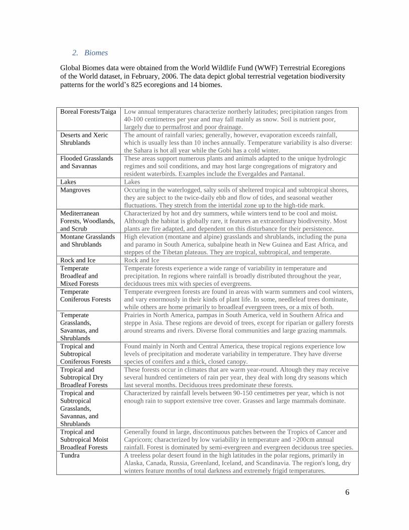
2. Biomes

Global Biomes data were obtained from the World Wildlife Fund (WWF) Terrestrial Ecoregions

of the World dataset, in February, 2006. The data depict global terrestrial vegetation biodiversity

patterns for the world’s 825 ecoregions and 14 biomes.

Boreal Forests/Taiga Low annual temperatures characterize northerly latitudes; precipitation ranges from

40-100 centimetres per year and may fall mainly as snow. Soil is nutrient poor,

largely due to permafrost and poor drainage.

Deserts and Xeric

Shrublands

The amount of rainfall varies; generally, however, evaporation exceeds rainfall,

which is usually less than 10 inches annually. Temperature variability is also diverse:

the Sahara is hot all year while the Gobi has a cold winter.

Flooded Grasslands

and Savannas

These areas support numerous plants and animals adapted to the unique hydrologic

regimes and soil conditions, and may host large congregations of migratory and

resident waterbirds. Examples include the Evergaldes and Pantanal.

Lakes Lakes

Mangroves Occuring in the waterlogged, salty soils of sheltered tropical and subtropical shores,

they are subject to the twice-daily ebb and flow of tides, and seasonal weather

fluctuations. They stretch from the intertidal zone up to the high-tide mark.

Mediterranean

Forests, Woodlands,

and Scrub

Characterized by hot and dry summers, while winters tend to be cool and moist.

Although the habitat is globally rare, it features an extraordinary biodiversity. Most

plants are fire adapted, and dependent on this disturbance for their persistence.

Montane Grasslands

and Shrublands

High elevation (montane and alpine) grasslands and shrublands, including the puna

and paramo in South America, subalpine heath in New Guinea and East Africa, and

steppes of the Tibetan plateaus. They are tropical, subtropical, and temperate.

Rock and Ice Rock and Ice

Temperate

Broadleaf and

Mixed Forests

Temperate forests experience a wide range of variability in temperature and

precipitation. In regions where rainfall is broadly distributed throughout the year,

deciduous trees mix with species of evergreens.

Temperate

Coniferous Forests

Temperate evergreen forests are found in areas with warm summers and cool winters,

and vary enormously in their kinds of plant life. In some, needleleaf trees dominate,

while others are home primarily to broadleaf evergreen trees, or a mix of both.

Temperate

Grasslands,

Savannas, and

Shrublands

Prairies in North America, pampas in South America, veld in Southern Africa and

steppe in Asia. These regions are devoid of trees, except for riparian or gallery forests

around streams and rivers. Diverse floral communities and large grazing mammals.

Tropical and

Subtropical

Coniferous Forests

Found mainly in North and Central America, these tropical regions experience low

levels of precipitation and moderate variability in temperature. They have diverse

species of conifers and a thick, closed canopy.

Tropical and

Subtropical Dry

Broadleaf Forests

These forests occur in climates that are warm year-round. Altough they may receive

several hundred centimeters of rain per year, they deal with long dry seasons which

last several months. Deciduous trees predominate these forests.

Tropical and

Subtropical

Grasslands,

Savannas, and

Shrublands

Characterized by rainfall levels between 90-150 centimetres per year, which is not

enough rain to support extensive tree cover. Grasses and large mammals dominate.

Tropical and

Subtropical Moist

Broadleaf Forests

Generally found in large, discontinuous patches between the Tropics of Cancer and

Capricorn; characterized by low variability in temperature and >200cm annual

rainfall. Forest is dominated by semi-evergreen and evergreen deciduous tree species.

Tundra A treeless polar desert found in the high latitudes in the polar regions, primarily in

Alaska, Canada, Russia, Greenland, Iceland, and Scandinavia. The region's long, dry

winters feature months of total darkness and extremely frigid temperatures.

7

Source Information: http://www.worldwildlife.org/science/ecoregions/terrestrial.cfm. See also

Olson, D.M., E. Dinerstein, E.D. Wikramanayake, N.D. Burgess, G.V.N. Powell, E.C.

Underwood, J.A. D'Amico, H.E. Strand, J.C. Morrison, C.J. Loucks, T.F. Allnutt, J.F. Lamoreux,

T.H. Ricketts, I. Itoua, W.W. Wettengel, Y. Kura, P. Hedao, and K. Kassem. 2001. Terrestrial

ecoregions of the world: A new map of life on Earth. BioScience 51(11): 933-938.

3. Climate Zones

Köppen-Geiger Climate Classification maps of the world, from the Vienna Institute of Veterinary

Public Health, were selected to represent global climatological regions based on observed climate

data for the period 1976-2000, as well as projected climate shifts in accordance with 4 emissions

scenarios (A1F1, A2, B1, and B2) developed by the Intergovernmental Panel on Climate Change

(IPCC), and described in the Special Report of Emission Scenarios (SRES) for the period 2001 –

2025. The Köppen-Geiger system is based on annual and monthly averages of temperature and

precipitation ranges.

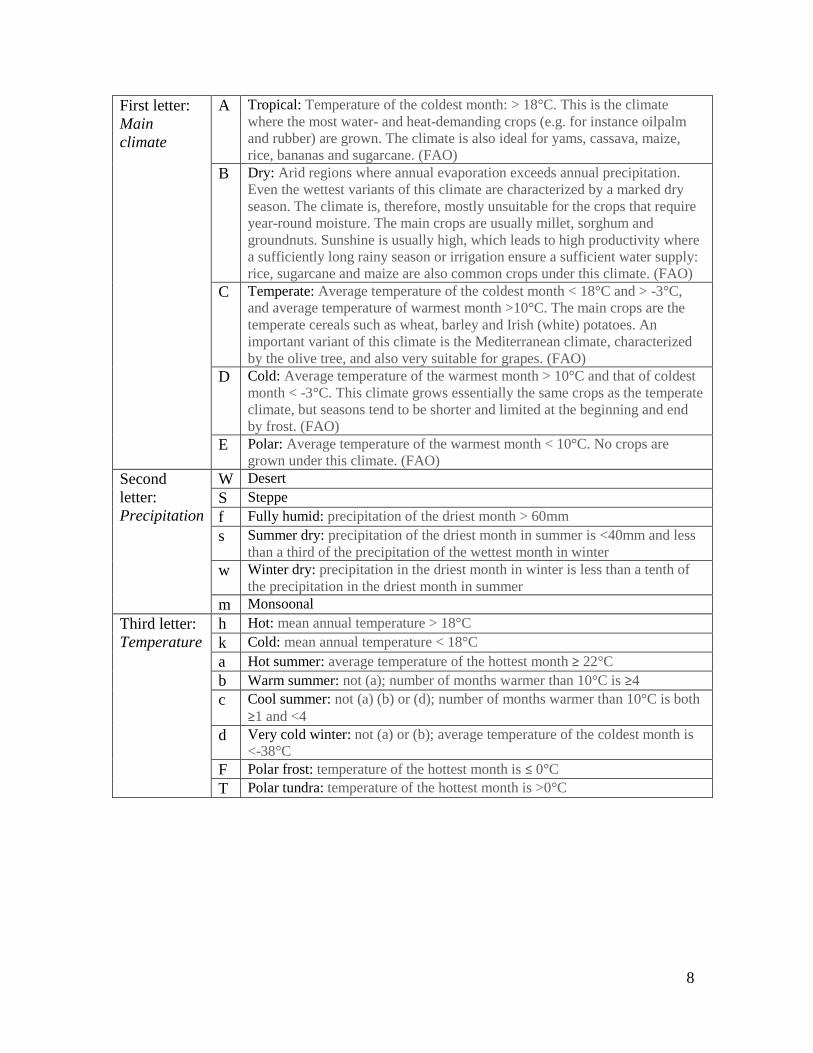
Climate zones are grouped into 5 super categories, based on general annual distributions of

temperature and rainfall. Tropical systems are coded as ―A‖, Dry systems as ―B‖, Temperate

systems as ―C‖, Cold systems as ―D‖ and Polar systems as ―E‖. Each of these 5 main classes

contains combinations of subclass identifiers, based on seasonality, precipitation and temperature

patterns. These classifications are reflected in climate zone abbreviations, which are composed of

three letters.

The emissions scenarios are as follows, defined by the Intergovernmental Panel on Climate

Change (IPCC) and described by the Special Report on Emissions Scenarios (SRES):

A1: (F1: fossil fuel intensive) quick economic growth, quick launch of new and efficient

technologies

A2: very heterogenic world with focus on family values and local traditions

B1: a world without materialism and launch of clean technologies

B2: focus on local solutions for economic and ecological sustainability

Source Information: FAO's Sustainable Development Department (SD). 2006. Global Climate

Maps. Köeppen Climate Classification Map (http://www.fao.org/sd/EIdirect/climate/

EIsp0002.htm) and ―Brief guide to Koeppen Climate classification system‖

(http://www.fao.org/sd/EIdirect/climate/EIsp0066.htm).

See also:

Rubel, F., and M. Kottek, 2010. Observed and projected climate shifts 1901-2100 depicted by

world maps of the Köppen-Geiger climate classification. Meteorol. Z., 19, 135-141

(http://koeppen-geiger.vu-wien.ac.at/shifts.htm).

Peel, M. C., Finlayson, B. L., and McMahon, T. A. 2007. Updated world map of the Köppen-

Geiger climate classification, Hydrol. Earth Syst. Sci., 11, 1633-1644, doi:10.5194/hess-11-1633-

2007 (http://www.hydrol-earth-syst-sci.net/11/1633/2007/hess-11-1633-2007.pdf).

IPCC SRES (2000), Nakićenović, N., and Swart, R., ed. (book), Special Report on Emissions

Scenarios: A special report of Working Group III of the Intergovernmental Panel on Climate

Change, Cambridge University Press.

8

First letter:

Main

climate

A Tropical: Temperature of the coldest month: > 18°C. This is the climate

where the most water- and heat-demanding crops (e.g. for instance oilpalm

and rubber) are grown. The climate is also ideal for yams, cassava, maize,

rice, bananas and sugarcane. (FAO)

B Dry: Arid regions where annual evaporation exceeds annual precipitation.

Even the wettest variants of this climate are characterized by a marked dry

season. The climate is, therefore, mostly unsuitable for the crops that require

year-round moisture. The main crops are usually millet, sorghum and

groundnuts. Sunshine is usually high, which leads to high productivity where

a sufficiently long rainy season or irrigation ensure a sufficient water supply:

rice, sugarcane and maize are also common crops under this climate. (FAO)

C Temperate: Average temperature of the coldest month < 18°C and > -3°C,

and average temperature of warmest month >10°C. The main crops are the

temperate cereals such as wheat, barley and Irish (white) potatoes. An

important variant of this climate is the Mediterranean climate, characterized

by the olive tree, and also very suitable for grapes. (FAO)

D Cold: Average temperature of the warmest month > 10°C and that of coldest

month < -3°C. This climate grows essentially the same crops as the temperate

climate, but seasons tend to be shorter and limited at the beginning and end

by frost. (FAO)

E Polar: Average temperature of the warmest month < 10°C. No crops are

grown under this climate. (FAO)

Second

letter:

Precipitation

W Desert

S Steppe

f Fully humid: precipitation of the driest month > 60mm

s Summer dry: precipitation of the driest month in summer is <40mm and less

than a third of the precipitation of the wettest month in winter

w Winter dry: precipitation in the driest month in winter is less than a tenth of

the precipitation in the driest month in summer

m Monsoonal

Third letter:

Temperature

h Hot: mean annual temperature > 18°C

k Cold: mean annual temperature < 18°C

a Hot summer: average temperature of the hottest month ≥ 22°C

b Warm summer: not (a); number of months warmer than 10°C is ≥4

c Cool summer: not (a) (b) or (d); number of months warmer than 10°C is both

≥1 and <4

d Very cold winter: not (a) or (b); average temperature of the coldest month is

<-38°C

F Polar frost: temperature of the hottest month is ≤ 0°C

T Polar tundra: temperature of the hottest month is >0°C

9

4. Coastal Proximity Zones

Coastal proximity zones are inland regions within 5, 10, 100, or 200 kilometers of the GRUMPv1

shoreline (see source information for GRUMPv1). These were derived by CIESIN.

5. Elevation Zones

ISciences LLC’s digital elevation data is a 1 km raster that combines NASA's Shuttle Radar

Topographic Mission data with bathymetric values to produce a land elevation and marine depth

layer. 12 thematic zones were created by aggregating elevation values.

Zones (meters): less than 5 meters, 5-10m, 10-25m, 25-50m, 50-100m, 100-200m, 200-400m,

400-800m, 800-1500m, 1500-3000m, 3000-5000m, higher than 5000m.

Source Information: Elevation and Depth Map – 30 arc-seconds, available at

http://www.terraviva.net/datasolutions/projects_elevation.html. For further information

contact: ISciences, L.L.C. 300 N. Fifth Ave. Suite 120., Ann Arbor, MI 48104.

6. Population Density Zones

Population Density layers, for 1990, 2000, and 2010 were created by dividing the 1990, 2000, and

2010 UN-adjusted population (POP) count grids by the land area (LA) grid. Population and area

grids are from GRUMP v1 (see source information for GRUMPv1).

Twelve thematic zones were created by aggregating population density values.

Zones (persons per square kilometer): 0, 1-2, 3-5, 6-10, 11-15, 16-50, 51-100, 101-500, 501-

1000, 1001-10000, 10001-50000, greater than 50000.

10

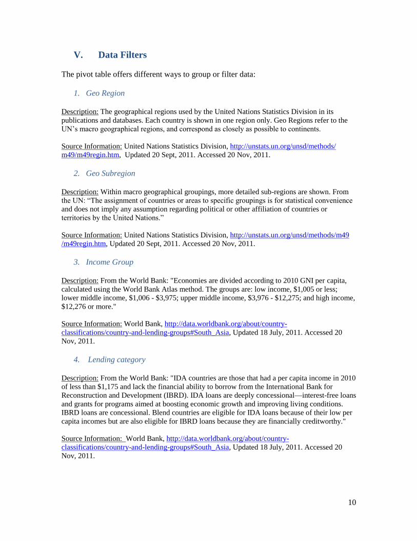
V. Data Filters

The pivot table offers different ways to group or filter data:

1. Geo Region

Description: The geographical regions used by the United Nations Statistics Division in its

publications and databases. Each country is shown in one region only. Geo Regions refer to the

UN’s macro geographical regions, and correspond as closely as possible to continents.

Source Information: United Nations Statistics Division, http://unstats.un.org/unsd/methods/

m49/m49regin.htm, Updated 20 Sept, 2011. Accessed 20 Nov, 2011.

2. Geo Subregion

Description: Within macro geographical groupings, more detailed sub-regions are shown. From

the UN: ―The assignment of countries or areas to specific groupings is for statistical convenience

and does not imply any assumption regarding political or other affiliation of countries or

territories by the United Nations.‖

Source Information: United Nations Statistics Division, http://unstats.un.org/unsd/methods/m49

/m49regin.htm, Updated 20 Sept, 2011. Accessed 20 Nov, 2011.

3. Income Group

Description: From the World Bank: "Economies are divided according to 2010 GNI per capita,

calculated using the World Bank Atlas method. The groups are: low income, $1,005 or less;

lower middle income, $1,006 - $3,975; upper middle income, $3,976 - $12,275; and high income,

$12,276 or more."

Source Information: World Bank, http://data.worldbank.org/about/country-

classifications/country-and-lending-groups#South_Asia, Updated 18 July, 2011. Accessed 20

Nov, 2011.

4. Lending category

Description: From the World Bank: "IDA countries are those that had a per capita income in 2010

of less than $1,175 and lack the financial ability to borrow from the International Bank for

Reconstruction and Development (IBRD). IDA loans are deeply concessional—interest-free loans

and grants for programs aimed at boosting economic growth and improving living conditions.

IBRD loans are concessional. Blend countries are eligible for IDA loans because of their low per

capita incomes but are also eligible for IBRD loans because they are financially creditworthy."

Source Information: World Bank, http://data.worldbank.org/about/country-

classifications/country-and-lending-groups#South_Asia, Updated 18 July, 2011. Accessed 20

Nov, 2011.

11

5. Urban/Rural Designation

Description: The urban extent filter distinguishes urban and rural areas based on a combination of

population counts (persons), settlement points, and the presence of Nighttime Lights. Areas are

defined as urban where contiguous lighted cells from the Nighttime Lights or approximated urban

extents based on buffered settlement points for which the total population is greater than 5,000

persons.

Source Information: Columbia University Center for International Earth Science Information

Network (CIESIN) in collaboration with the International Food Policy Research Institute (IFPRI),

The World Bank, and Centro Internacional de Agricultura Tropical (CIAT). GRUMPv1 Urban

Extents Dataset, http://sedac.ciesin.columbia.edu/gpw/global.jsp, Accessed 20 Nov, 2011.

12

VI. Data Processing and Methodology

Overview – Basic Methods

All data were assigned to a Geographic (WGS84) coordinate system and resampled to

match the 30 arc-second grid format, and resolution (approximately 1km2 at the equator)

of the GRUMPv1 Population (POP), Administrative Boundary (ADM), Urban Extents

(UR), and Land Area (LA) grids. Coastal boundaries were reconciled to conform to the

GRUMPv1 coastlines.

Combined grids were derived by overlaying classes within each thematic variable,

(Density Zones, Coastal Proximity Zones, Climate Zones, Elevation Zones and Biomes)

with GRUMPv1 country boundaries. This returned layers of the classes for each input

grid, organized by country.

Since the comparisons were run at the cell level, population and land area values could be

queried for each pixel, from the underlying POP (1990, 2000, and 2010) and LA layers.

The GRUMPv1 UR data was used to subset the POP and LA layers into Urban and Rural

designations. Zonal statistics were summed and reported for population and land area,

by thematic class, by country, by UR zone.

Data Specific Methods

National Boundaries, Shorelines, Population, Urban Extents, Land Area, Population

Density Classes

The suite of Global Rural-Urban Mapping Project, version 1 (GRUMPv1) datasets served as base

spatial inputs for all assessments. GRUMPv1 data includes, among others, global estimates of

human population for the years 1990, and 2000, formatted in 30 arc-second grid cells. Population

values for GRUMPv1 were calculated using a proportional allocation gridding algorithm;

populations were distributed in greater proportion to urban areas, and at a lesser rate to rural

areas. Population estimates for 2010 were derived by scaling GRUMPv1 2000 by the HYDEv3.1

database. Urban and rural area designations were determined by use of the Defense

Meteorological Satellite Program (DMSP) Operational Linescan System (OLS) ―night-time

lights‖ dataset, and city-level census data.

See http://sedac.ciesin.columbia.edu/gpw/docs/UR_paper_webdraft1.pdf for a full description.

Because most countries’ national statistical offices report census data values that differ from

United Nations population estimates, GRUMPv1 data are made available as either adjusted to the

UN estimates or in their unadjusted form. For the UN adjustment, a national-level conversion

factor representing the difference between the estimates from each national statistical office and

the UN estimate is applied to the population values. The UN adjusted data were used for all

population calculations in PLACE III. Users wishing to utilize unadjusted population values can

find the conversion factors used for each country at:

http://sedac.ciesin.columbia.edu/gpw/spreadsheets/GPW3_GRUMP_SummaryInformation_Oct0

5prod.xls (see Excel page Codebook).

13

Population

PLACE III updates use the GRUMP v1 UN-adjusted population values from 1990, 2000, and

scales the GRUMPv1 2000 estimates by the HYDEv3.1 population rates to produce estimates for

year 2010. Population totals for each country were calculated using a GIS overlay process. Total

POP values for all pixels that overlap those for each unique ADM value were summarized by UR

zone, and total coverage, for each of the 1990, 2000, and 2010 POP layers. Per class percentages

were calculated as fractions of this summarized value. Regions where input layers did not contain

values (most often true of smaller, island nations), are presented as Missing Data. The sum of all

per class percentages, by country, together with the Missing Data values, will equal 100 percent

of the GIS calculated POP. While real-world country boundaries changed during the 1990 to

2010 period, for the sake of consistency, we employed a uniform ADM geography for all

analyses; that of the circa 2000 layer.

Land Area

The GRUMPv1 global Land Area (LA) grid was used for calculating the size (square km) and

percentage land area, per class, by country, by UR zone, for each input layer. The GRUMPv1 LA

grid has been calibrated to more precisely represent the actual per cell area (sq.km), which varies

by latitude. As per POP, the total LA values for pixels matching those for a particular ADM unit,

and UR zone within the unit, were summarized using a GIS overlay process. Per class

percentages, by country by UR designation, were calculated as fractions of this summed national

value. Areas where input layers did not contain spatial information consistent with those regions

grown to match GRUMPv1 extents are presented as Missing Data. The total of per class values,

together with Missing Values, will equal 100 percent of the GIS calculated area. Large inland

water bodies and permanent ice have been removed from the analysis.

Biomes

Global Biomes data were obtained from the World Wildlife Fund (WWF) Terrestrial Ecoregions

of the World dataset, in February, 2006. The data are distributed in vector format, which were

created to be used at the scale of 1:1 million. CIESIN converted the data to raster grid format at a

30 arc-second resolution and clipped to match the extent of GRUMP v1.

Climate Zones

The Köppen-Geiger Climate Classification system was selected to represent global climatological

regions. The classification system is based on annual and monthly averages of temperature and

precipitation ranges. For observed data, two separate data sets were used; the Climatic Research

Unit (CRU) of the University of East Anglia (Mitchell and Jones, 2005) for temperature, and the

Global Precipitation Climatology Centre (GPCC) Full Data Reanalysis Version 4 for 1901 to

2007 (Fuchs, 2008) for precipitation. For projected data, the Tyndall Centre for Climate Change

Research data set, TYN SC 2.03 (Mitchell et al., 2004) was used. From here data was averaged

over periods of 25 years. These results show ensemble-means runs against 5 global climate

model (GCM) projections illustrating 4 emissions scenarios described by the IPCC. Map data

were received by CIESIN as 0.5 degree ascii grids, in a Geographic projection. They were

converted into ESRI GRID format and resampled, using a nearest neighbor algorithm, to match

the extent and resolution of GRUMPv1.

14

Coastal Proximity Zones

Coastal proximity zones (regions within 5km, 10km, 100km, or 200km of a coast) were created

from the GRUMPv1 shoreline vector layer. The vector layer was first converted into points and

densified, then geodesic buffers (5km, 10km, 100km, and 200km) were created from shoreline

vertices and dissolved into polygon features, finally, the polygons were clipped to include just the

inland portions of the buffer zones.

Elevation Zones

Digital elevation data were obtained as a 1 kilometer resolution elevation\bathymetry raster

product from ISciences, L.L.C. (http://www.isciences.com/). Elevation zones were created by

aggregating ranges of land elevation values into 12 thematic elevation classes, as described

below. ISciences’ TerraViva! product combines NASA’s Shuttle Radar Topographic Mission

(SRTM30) digital elevation data with bathymetric values to produce a seamless, globally

consistent land elevation and marine depth layer. Gaps and voids in the original SRTM (v1) data

were supplemented by elevation data layers from the NOAA GLOBE project

(http://www.ngdc.noaa.gov/mgg/topo/globe.html) to provide a high-quality global coverage of all

land surface areas.

Population Density Zones

Population Density layers, for 1990, 2000, and 2010 were created by dividing the 1990, 2000, and

2010 UN-adjusted population (POP) count grids by the land area (LA) grid. The pixel values for

the resulting grid layers, one each for 1990, 2000, and 2010, were then aggregated to form the 12

population density classes.

15

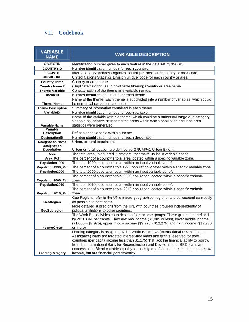
VII. Codebook

VARIABLE NAME

VARIABLE DESCRIPTION

OBJECTID Identification number given to each feature in the data set by the GIS.

COUNTRYID Number identification, unique for each country.

ISO3V10 International Standards Organization unique three-letter country or area code. UNSDCODE United Nations Statistics Division unique code for each country or area.

Country Name Country or area name

Country Name 2 (Duplicate field for use in pivot table filtering) Country or area name

Theme: Variable Concatenation of the theme and variable names.

ThemeID Number identification, unique for each theme.

Theme Name

Name of the theme. Each theme is subdivided into a number of variables, which could be numerical ranges or categories.

Theme Description Summary of information contained in each theme.

VariableID Number identification, unique for each variable

Variable Name

Name of the variable within a theme, which could be a numerical range or a category. Variable boundaries delineated the areas within which population and land area statistics were generated.

Variable Description Defines each variable within a theme.

DesignationID Number identification, unique for each designation.

Designation Name Urban, or rural population. Designation Description Urban or rural location are defined by GRUMPv1 Urban Extent.

Area The total area, in squared kilometers, that make up input variable zones.

Area_Pct The percent of a country’s total area located within a specific variable zone.

Population1990 The total 1990 population count within an input variable zone*.

Population1990_Pct The percent of a country’s total1990 population located within a specific variable zone.

Population2000 The total 2000 population count within an input variable zone*.

Population2000_Pct

The percent of a country’s total 2000 population located within a specific variable zone.

Population2010 The total 2010 population count within an input variable zone*.

Population2010_Pct

The percent of a country’s total 2010 population located within a specific variable zone.

GeoRegion

Geo Regions refer to the UN’s macro geographical regions, and correspond as closely as possible to continents.

GeoSubregion

More detailed subregions from the UN, with countries grouped independently of political affiliations to other countries.

IncomeGroup

The Work Bank divides countries into four income groups. These groups are defined by 2010 GNI per capita. They are: low income ($1,005 or less), lower middle income ($1,006 – $3,975), upper middle income ($3,976 - $12,275) and high income ($12,276 or more)

LendingCategory

Lending category is assigned by the World Bank. IDA (International Development Assistance) loans are targeted interest-free loans and grants reserved for poor countries (per capita income less than $1,175) that lack the financial ability to borrow from the International Bank for Reconstruction and Development. IBRD loans are noncessional. Blend countries qualify for both types of loans – these countries are low-income, but are financially creditworthy.

16

VIII. Acknowledgment

Funding for this dataset was provided under the U.S. National Aeronautics and Space

Administration (NASA) Socioeconomic Data and Applications Center (SEDAC) contract

NAS5-98162 to the Center for International Earth Science Information Network

(CIESIN) of Columbia University. We wish to thank the hard, dedicated work of the

many CIESIN staff that made completion of this update possible.

IX. Disclaimer

CIESIN provides this data without any warranty of any kind whatsoever either expressed

or implied. CIESIN shall not be liable for incidental, consequential, or special damages

arising out of the use of any data provided by CIESIN. No third-party distribution of all

or parts of this dataset are permitted without permission.

These data are for noncommercial use; commercial use is not permitted without explicit

permission. Additionally, users of the data should acknowledge CIESIN as the source

used in the creation of any reports, publications, new data sets, derived products, or

services resulting from their use. CIESIN also requests reprints of any publications

acknowledging CIESIN as the source and requests notification of any redistribution

efforts. The Trustees of Columbia University in the City of New York hold the copyright

on data created at CIESIN. CIESIN obtains permissions to disseminate data produced by

others. Intellectual property rights and permissions associated with each particular data

set are specified in the documentation of the data.