Population Dynamics With Resources

8/14/2019 Population Dynamics With Resources

http://slidepdf.com/reader/full/population-dynamics-with-resources 1/38

Preprint LDC-2009-002, Rev. 11/8/2010

A SIMPLE POPULATION DYNAMICS MODEL

WITH RESOURCE LIMITS

Lawrence D. Cloutman

[email protected]

Abstract

The commonly used logistic model of population dynamics predicts a monotonicpopulation rise up to the carrying capacity and a constant population thereafter. Wemodify the logistic model to include a simple model to account for the resources nec-essary to support the p opulation. The resources are modeled by a lumped “energy”variable that represents a combination of renewable and nonrenewable resources. Theresulting third order Lotka-Volterra equations are solved numerically for a variety of conditions. Populations that are too dependent on nonrenewable resources collapse andnever fully recover, leveling off at a nearly constant level determined by the availability

of renewable resources.

c2010 by Lawrence D. Cloutman. All rights reserved .

1



1 Introduction

The commonly used logistic model of population dynamics predicts a monotonic population

rise up to the carrying capacity and a constant population thereafter. The factor that limits

the population is not specified, but often is attributed to some variation on the themes of

famine, pandemic, predation, and warfare. This lack of specificity of the mechanism forpopulation limitation is reflected in the simplistic ad hoc nonlinear term in the logistic

equation. To make the logistic model more realistic, we modify it to include a simple

model for a finite resource necessary to support the population. This is accomplished by

introducing an energy variable with renewable and nonrenewable components. This variable

is a surrogate for such disparate items as food, water, and fossil fuels. The resulting third

order Lotka-Volterra equations are solved numerically for a selected set of conditions.

The next section presents the logistic equation. Section 3 describes the extension

of the logistic model to include an energy variable. Section 4 contains numerical examples.

Section 5 contains the conclusions. The appendix explores the connection between numerical

instabilities in finite difference approximations to the logistic equation and chaos in iterated

maps.

2



3 A Simple Resource Model

The simplistic logistic model easily can be made more realistic by including effects found in

real ecosystems. One key effect is the dependence of the population upon certain resources,

which can be either renewable or nonrenewable. We choose to express this resource in

terms of an energy variable, E (t). This lumped variable will include everything necessary tomaintain the population at its chosen rate of consumption, including food, fuels, and goods

of all kinds. E is available for immediate use, or it may be stockpiled for future use. 1 It

includes only forms of “energy” available for use upon demand. We assume E ≥ 0 obeys the

differential equationdE

dt= MNH (C ) + S 0 + S 1N − UN, (4)

where M , S 0, S 1, and U are constants.

The variable C (t) represents some nonrenewable source of E (such as coal, other fossil

fuels, or underground irrigation water) that requires mining, pumping, or some other kindof processing to be converted into E . We assume that the variable C obeys the differential

equationdC

dt= −MNH (C ). (5)

This equation represents the conversion of the resource C into available energy E , so the

negative of the right-hand side of equation (5) appears as a source of E in equation (4).

The function H (C ) ≥ 0 is introduced to represent the fact that once the nonre-

newable resource C is depleted, it is no longer available as an energy source and never will

be again. It should have the properties that at t = 0, H (C ) = 1, and that for C = 0,H (C ) = 0. While the precise form of this function is not known in general, it should have

the additional property that for large values of C , its value should be near unity to represent

the relative ease of converting C into E . As C is depleted, production becomes more difficult

or expensive, and H (C ) should decrease. The ad hoc assumption that we shall use in this

study is

H (C ) = [C (t)/C (0)]ω if C > 0

= 0 if C ≤ 0, (6)

where ω is a nonnegative constant. We shall consider the cases with ω = 0, 0.25, and 1 in

this study. The first case reduces to the Heaviside function, which is a step function that

switches between zero and unity at C = 0. This would be appropriate for a resource, such

as grain in a bin, that is easy to extract down to the last grain. However, some resources,

1While this model is sufficiently general to apply to many species, our discussion, and therefore thelanguage used, will be slanted toward human population dynamics.

4



The combined population/resource model is equations (1) plus (4) through (8). The

model comprises three first-order differential equations, nine constants, and initial values for

N , C , and E .

Table 1. Constants for Numerical Examples

Constant Cases 1-3 Case 4 Case 5 Case 6 Case 7 Case 8

A+ 0.03 0.03 0.03 0.03 0.03 0.03A− 0.06 0.06 0.06 0.06 0.02 0.02B 3.0 × 10−12 3.0 × 10−12 3.0 × 10−12 3.0 × 10−12 3.0 × 10−12 3.0 × 10−12

M 0.6 0.6 0.6 0.6 0.6 0.1S 0 1.0 × 108 1.0 × 108 3.0 × 108 3.0 × 108 3.0 × 108 3.0 × 108

S 1 0.5 0.5 0.5 0.5 0.5 0.5

α 0.7 0.7 0.7 0.35 0.35 0.35U 1.0 1.0 1.0 1.0 1.0 1.0ω 0.0, 0.25, 1.0 0.25 0.25 0.25 0.25 0.25

C (0) 1.0 × 1011 2.0 × 1011 2.0 × 1011 2.0 × 1011 2.0 × 1011 2.0 × 1011

E (0) 1.2 × 106 2.4 × 106 2.4 × 106 2.4 × 106 2.4 × 106 2.4 × 106

N (0) 1.0 × 106 1.0 × 106 1.0 × 106 1.0 × 106 1.0 × 106 1.0 × 106

6



4 Examples

The model equations are nonlinear and must be solved numerically. The numerical integra-

tions were performed with a standard second-order Runge-Kutta technique discussed in the

appendix.

We shall consider several cases whose parameter values are listed in table 1. Thefirst three cases differ only in the value of ω. Historically, human populations have increased

around 3 percent per year, so we take A+ = 0.03. We know the logistic carrying capacity is

greater than 6 × 109, so let’s take it to be K = 1.0 × 1010. That fixes B = 3.0 × 10−12. We

shall assume our population lives a reasonable but modest lifestyle, with α = 0.7, and we

shall assume U = 1.0 energy units per capita per year. 3 We assume the resource parameters

M = 0.6 energy units per capita per year, S 0 = 1.0 × 108 energy units per year, and S 1 = 0.5

energy units per capita per year. Initial conditions are N (0) = 1.0 × 106, E (0) = 1.2 × 106

energy units, and C (0) = 1.0 × 1011 energy units.

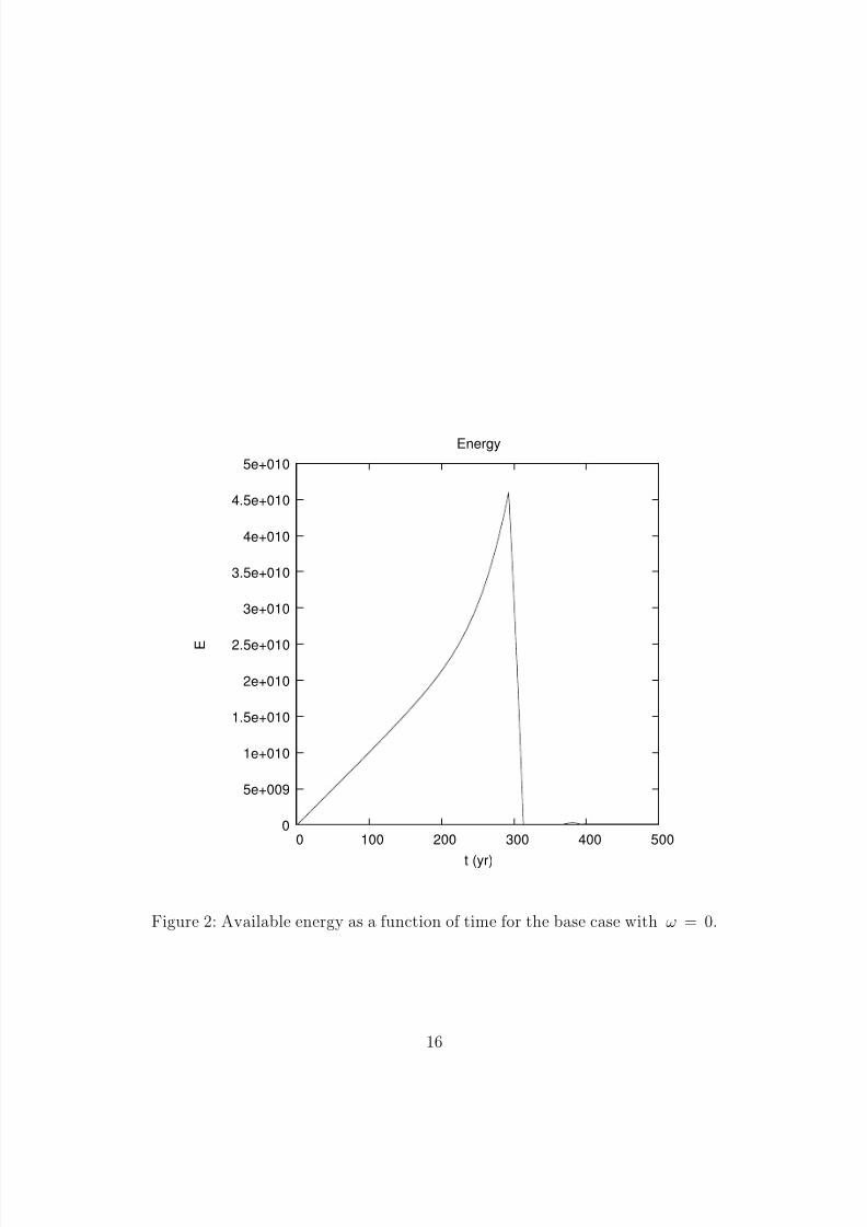
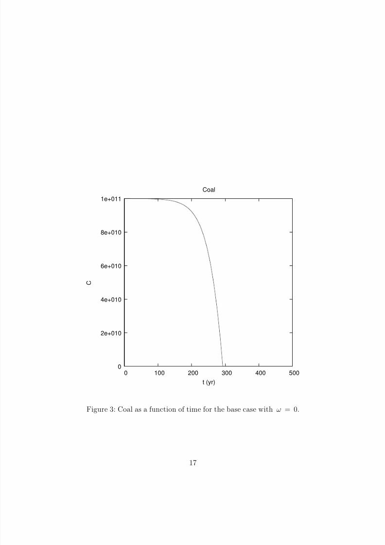
Figure 1 shows the population as a function of time for case 1, the model with

ω = 1. Figure 2 shows E (t), and figure 3 shows C (t). For the first 300 years, population

and energy supplies grow exponentially, as does the depletion rate of C . Finally, C is depleted

and E drops as renewable resources cannot supply enough to sustain the population. The

population crashes to a level that can be sustained by renewable resources. Note that the

population never reaches the logistic carrying capacity.

Even though this population model appears to be a third order system of equations,

it cannot have chaotic solutions. The variable C decays monotonically to zero and stays

there. Therefore, the solution vector (N , E , C ) will have orbits only in the two-dimensionalC = 0 plane at late times. This collapse of the solution space to two dimensions effectively

reduces the system of equations to second order.

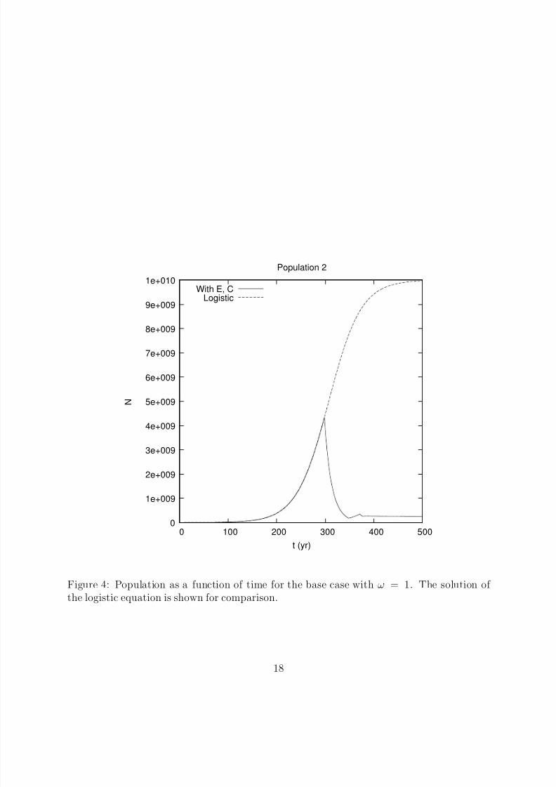
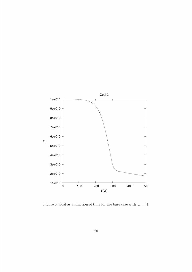
Figures 4 through 6 show the analogous plots for case 2, ω = 1. Figures 7 through

9 show the analogous plots for case 3, ω = 0.25. There is very little difference among the

first three cases, implying an insensitivity to the exact form of H (C ). The only qualitative

difference is that C (t) is not completely depleted before the population crash in case 2.

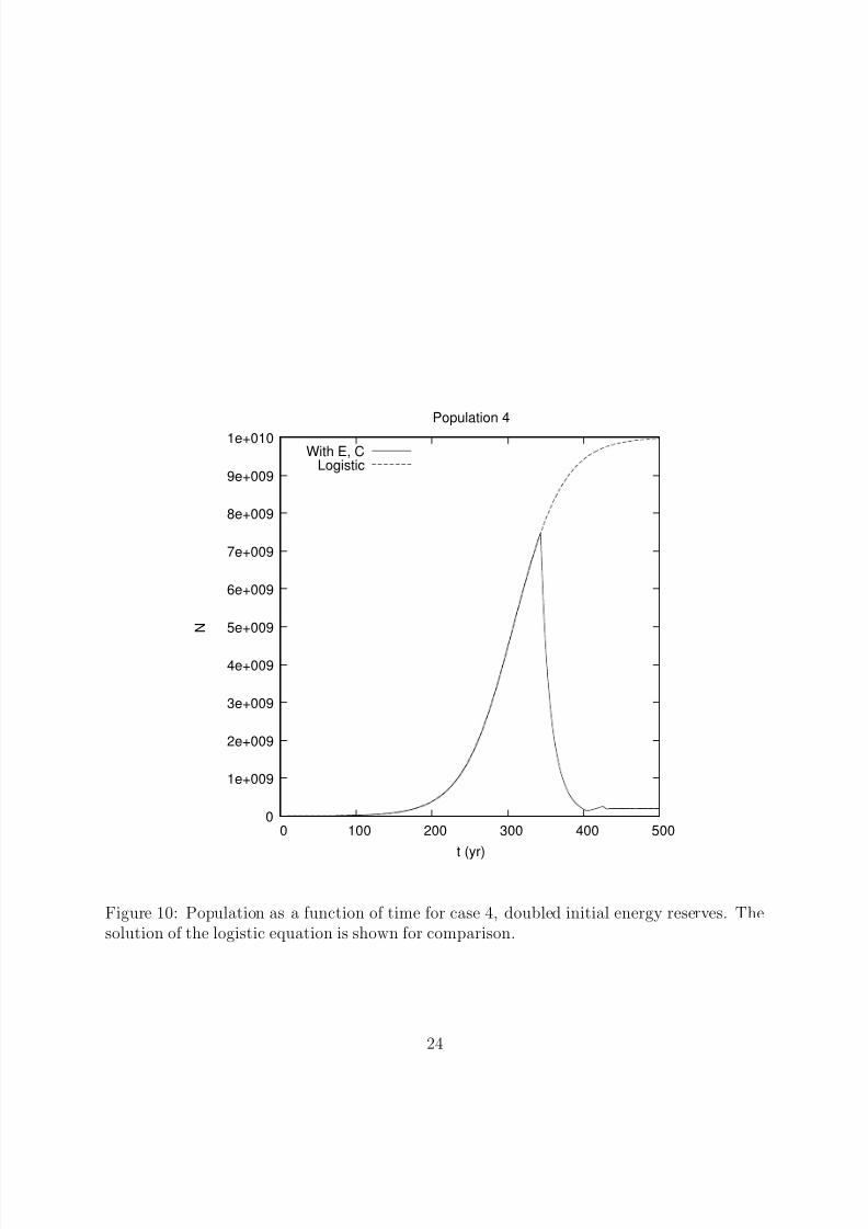
Case 4 is the same as case 3 except E (0) and C (0) were doubled to increase the

energy stores available to the population. This delayed the population crash by only about

50 years, but did not change the final sustainable population of about 200 million.

Case 5 is the same as case 4 except S 0 was tripled. This change delays the crash for

about 20 more years, so the population has time to grow further up the logistic curve. It

3This choice for U defines the unit of energy. It is left up to the reader to specify the average numberof joules or BTUs or other conventional energy units each person uses in one year, which is the conversionfactor between my arbitrary “energy units” and conventional physical units.

7



also increases the sustainable population by a factor of three. This behavior is exactly what

one would expect, that a population that has exhausted some critical nonrenewable resource

will be dependent upon how much renewable resource can be made available.

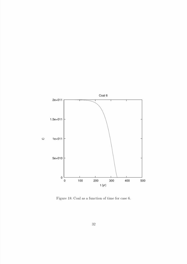
In case 6, α was reduced to 0.35. This represents a dramatic decrease in the amount

of energy used to just sustain life, which would be reflected in a decreased standard of living.

Surprisingly, the results in cases 5 and 6 are nearly identical.

Case 7 is the same as case 6 except A− is reduced by a factor of one third. This

represents a lower death rate during times of famine. The difference between the two cases

is that the population crash occurs over a period of a century rather than about 40 years.

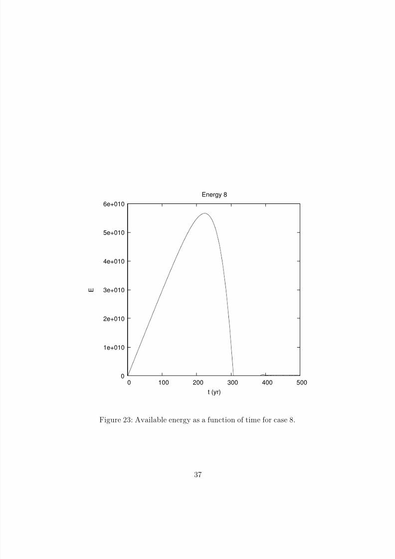
Case 8 is the same as case 7 except M has been reduced to 0.1. M may be interpreted

as the product of two factors. The first is the average rate at which one person can convert

C into E working full time. The second is the fraction of the population (in full-time

equivalents) engaged in that conversion activity. For example, these factors are how much

coal is mined by one miner and the fraction of people who are coal miners. Remember,however, that quantities such as M , E , and C represent a sum over all resources, not just

coal.

The results for case 8 are shown in figures 22 through 24. Comparing figures 19 and

22, we see that lowering M lowered the peak value of the population due to the reduced

production by conversion of C . Also, the crash occurs much earlier in time. Interestingly,

the post-crash population is slightly higher in figure 22.

In figure 23 the peak value of E is half that in figure 20. As in the other seven

cases, E goes to essentially zero after the crash. The surviving population is forced to rely

on renewables and any residual conversion production with little or no reserves of E . The

model assumes a constant rate of renewal of renewables. However, the population is now

vulnerable to further crashes due to interruption of production of renewables by factors not

included in the model, such as bad weather.

Figure 24 shows that instead of depleting C , only about a fourth of it is used in the

entire 500 years of the simulation. Figure 6 for case 2 is the only other plot of C that shows

a nonzero residual of C after the crash. In all cases, the population lives hand-to-mouth on

renewables and any residual C . It is this large residual that accounts for the slight elevation

of the post-crash population in case 8.In the context of the model, the key to avoiding a major population crash seems

to be the development of enough renewable resources to support some desired maximum

population well before the population reaches that value. However, that will work only if

the population does not use nonrenewables to allow overshooting the renewable carrying

capacity. Rerunning case 8 with M = 0 showed no significant change, so not relying heavily

8



on stockpiles of E while the population is below the renewables carrying capacity is crucial.

Case 8 was rerun with M and S 0 both reduced by a factor of 104. The population

started at 106 and monotonically decreased to a stable value of about 6 × 104. Increasing S 1

to 2.0 along with the reduced values of M and S 0 allowed the population to saturate near

the logistic carrying capacity. With S 1 = 1, the population grew slowly and monotonically

to 54 million over the 500 year span of the simulation, and it was still growing slowly due

to the slow accumulation of E . So, it is possible to avoid big population crashes by tuning

the parameters, but the price is to limit the growth of the population by limiting the use of

nonrenewables.

9



5 Conclusions

We have developed a simple extension of the logistic model of population dynamics that

includes the impact of finite renewable and nonrenewable resources. The results of numerical

experiments with this model may be summarized by the following conclusions.

1. A population that lives beyond its sustainable means will eventually crash when re-

sources are no longer available. This crash is a robust feature of the model.

2. The post-crash population stabilizes at a sustainable level determined by the availabil-

ity of renewable resources and conversion of any residual nonrenewables.

3. Regrowth of a depleted population is contingent upon creation of adequate renewable

resources.

4. The character of the solutions seems surprisingly insensitive to the parameter values,

most surprisingly to the value of α.

An obvious question is whether this model has any applicability to human population

dynamics. The model is simplistic in many ways, and computer models are not reality. The

model concentrates on approximating physical limits in terms of the flow of energy and ig-

nores many political and social factors. Furthermore, the present study has not thoroughly

explored the model’s parameter space. However, we seem to be moving inexorably into a

situation in which key resources are increasingly strained. These include petroleum, topsoil,

underground irrigation water, and a number of ocean fisheries. This development is suffi-

ciently worrying that it would be prudent to support further research into more detailed andrealistic models that may be used for insight and input into scientifically-based management

of ecological issues.

There are other resources that touch on the applicability question. One is an article

on critical aspects of continued growth as it impacts finite resources by Bartlett [9] While

the numbers he uses are somewhat dated, and while some of his most dire scenarios have

not come to pass, it would be a huge mistake to ignore his message about the implications

of continued population growth.

A second resource is the abundant material written about the history and ecology of

Rapa Nui (Easter Island). While many of the details are either unknown or controversial, the

ecological collapse on Rapa Nui is another lesson that should be neither ignored nor twisted to

fit any particular political, religious, academic, or moral agenda. If such events have lessons

for us, they must be uncovered in the light of fieldwork coupled with critical analysis and

reason rather than with wishful thinking or kneejerk emotionalism. A reasonable starting

place to get a broad overview of the issues is the Wikipedia article on-line.

10



A Instability and Chaos in Finite Difference Equations

Due to the nonlinearities in the differential equations, numerical methods must be used to

find approximate solutions. This introduces the issue of numerical stability of the methods

used. The stability of finite difference approximations to linear differential equations has been

well studied. In the case of nonlinear differential equations, they are sometimes linearizedand a stability analysis performed on the linearized equations [2]. Then one assumes the

results apply as well to the full nonlinear system. However, the stability conditions so derived

are only a necessary condition for numerical instability. In this section, we show that the

nonlinearities introduce additional considerations into the stability question.

The simplest explicit finite difference approximation to equation (2) is

N j+1 − N jδτ

= N j − N 2 j , (9)

where δτ is the dimensionless time step. It is easy to show that this approximation isconsistent. This equation may be rearranged to obtain

N j+1 = (1 + δτ ) N j − δτ N 2 j . (10)

If we apply the linear transformation M j = N j δτ /(1 + δτ ), we obtain

M j+1 = (1 + δτ )

M j − M2

j

≡ A

M j − M2

j

. (11)

This equation is just the familiar one-parameter logistic map with the parameter value

A = (1 + δτ ). Note that M has the value δτ /(1 + δτ ) for the nontrivial equilibrium solution N = 1, which is the same as the stable equilibrium solution of the logistic map, (A − 1)/A,

for 1 < A < 3.

The behavior of this map for various values of A has been thoroughly studied [3].

Assume we begin the iterations with 0 < M0 < 1.

1. For A less than unity, the map converges to zero monotonically.

2. For A between unity and two, the solution converges monotonically to N j = 1. This

corresponds to δτ < 1, which is the stability condition for the explicit method (9) to

produce a monotonically increasing solution.

3. For A between two and three, N j overshoots unity, then converges to unity, oscillating

about it on alternate cycles.

4. For A between 3 and 3.44, the solution eventually settles into a limit cycle with period

2.

11



5. For A between 3.44 and 3.57, the solution undergoes a sequence of period doublings.

6. For A between 3.57 and 4, the solution is chaotic.

7. For A greater than 4, the solution diverges to −∞.

Since the numerical integrations use A > 1, item 1 is never encountered in practice.Item 2 corresponds to the numerically stable situation which has the qualitatively correct

behavior of increasing monotonically with increasing j and therefore t. Linear stability theory

considers just two cases. The behavior is described by item 2 (stable) or item 7 (unstable,

with the numerical solution becoming unbounded). It is the presence of the nonlinearity that

introduces the complexities of items 3 through 6. This rich set of behaviors, in the context

of solving the differential equation, is unphysical even though the numerical solutions are

bounded and therefore will not cause the integration computer program to “crash” with an

overflow or NaN. This situation is a warning that studies based on numerical integrations

must always include grid refinement studies to insure the results converge to the solutionsof the underlying differential equations. That has been done in the present study, and only

the results using the smallest δτ ( ≤ 0.03) are presented.

The chaotic behavior is not confined to the explicit one-step difference equation (10).

Consider two second-order, two-step Runge-Kutta integration methods,

N ∗ − N j =δτ

2

N j − N 2 j

(12)

N j+1 − N j = δτ

N ∗ − N 2

∗ (13)

and

N ∗ − N j = δτ N j − N 2 j

(14)

N j+1 − N j =δτ

2

N j − N 2 j + N ∗ − N 2

∗

. (15)

The first method is based on the mid-point rule, and the second is based on the trapezoidal

rule. The results presented in this paper were computed with the second method.

Both methods have significant (< 32 percent) truncation errors for δτ = 1.05. So-

lutions from both methods are well-behaved (smooth and monotonic), and the mid-point

rule, equations (14)-(15), is slightly more accurate. However, both methods monotonically

approach the wrong steady state values (0.9756098 and 0.8780488) for δτ = 2.05. For

δτ = 3.05, the mid-point rule overshoots the equilibrium solution 0.6557377 and approaches

it with damped oscillations. The trapezoidal rule, on the other hand, goes into a period-4

limit cycle. At δτ = 4.05, both methods produce solutions that diverge to minus infinity.

These kinds of behavior have been reported elsewhere [4]- [7] for more complex numerical

methods.

12



Often partially implicit methods are used in practice, and there are numerous ways

the logistic equation can be approximated. Each particular difference approximation has

its own behavior, but typically there are a region of stability for small time steps, then

oscillatory and periodic solutions, chaotic solutions, and eventually solutions that become

unbounded. One of the most interesting partially implicit methods is

N j+1 − N jδτ

= N j+1 − N 2 j . (16)

For time steps less than 0.5, it is stable and the solution is monotonic. Since the explicit

method has well-behaved solutions out to a time step of unity, this shows that implicitness

does not always improve the size of the time step that one can use. Above a time step of

0.5, equation (16) has a rich and complex set of behaviors [8]. We will not go through the

entire list, but will note that there is some remarkable behavior for δτ between 0.74 and

0.76. At 0.74, the solution reaches a period-6 limit cycle that is almost-periodic with period

3. At 0.75, the solution is chaotic, and at 0.76 it becomes unbounded. The range of timestep that produces chaotic solutions is quite narrow. For still larger time steps, other types

of behavior can occur, including oscillations about zero.

13



References

[1] D. G. Cloutman and L. D. Cloutman, “A Unified Mathematical Framework for Popu-

lation Dynamics Modelling,” Ecol. Modelling 71 (1993) 131-160.

[2] R. D. Richtmyer, Difference Methods for Initial-Value Problems, Interscience Publishers,

NY, 1957.

[3] R. M. May, “Simple Mathematical Models With Very Complicated Dynamics,” Nature

261 (1976) 459-467.

[4] H. C. Yee, P. K. Sweby, and D. F. Griffiths, “Dynamical Approach Study of Spurious

Steady-State Numerical Solutions of Nonlinear Differential Equations. I. The Dynamics

of Time Discretization and Its Implications for Algorithm Development in Computa-

tional Fluid Dynamics,” J. Comput. Phys. 97, 249-310 (1991).

[5] H. C. Yee and P. K. Sweby, “The Dynamics of Some Iterative Implicit Schemes,” in

Chaotic Numerics, Contemporary Mathematics 172, (P. E. Kloeden and K. J. Palmer,

Eds.), American Mathematical Society, Providence, RI, 1994, pp. 75-96.

[6] H. C. Yee, J. R. Torczynski, S. A. Morton, M. R. Visbal, and P. K. Sweby, “On Spurious

Behavior of CFD Simulations,” AIAA Paper 97-1869 (1997).

[7] H. C. Yee and P. K. Sweby, “Aspects of Numerical Uncertainties in Time Marching to

Steady-State Numerical Solutions,” AIAA J. 36 (1998) 712-724.

[8] L. D. Cloutman, “A Note on the Stability and Accuracy of Finite Difference Approx-

imations to Differential Equations,” Lawrence Livermore National Laboratory report

UCRL-ID-125549, 1996.

[9] A. A. Bartlett, “Forgotten Fundamentals of the Energy Crisis,” Am. J. Phys. 46, 876

(1978).

14



0

1e+009

2e+009

3e+009

4e+009

5e+009

6e+009

7e+009

8e+009

9e+009

1e+010

0 100 200 300 400 500

N

t (yr)

Population

With E, CLogistic

Figure 1: Population as a function of time for the base case with ω = 0. The solution of the logistic equation is shown for comparison.

15



0

5e+009

1e+010

1.5e+010

2e+010

2.5e+010

3e+010

3.5e+010

4e+010

4.5e+010

5e+010

0 100 200 300 400 500

E

t (yr)

Energy

Figure 2: Available energy as a function of time for the base case with ω = 0.

16



0

2e+010

4e+010

6e+010

8e+010

1e+011

0 100 200 300 400 500

C

t (yr)

Coal

Figure 3: Coal as a function of time for the base case with ω = 0.

17



0

1e+009

2e+009

3e+009

4e+009

5e+009

6e+009

7e+009

8e+009

9e+009

1e+010

0 100 200 300 400 500

N

t (yr)

Population 2

With E, CLogistic

Figure 4: Population as a function of time for the base case with ω = 1. The solution of the logistic equation is shown for comparison.

18



0

5e+009

1e+010

1.5e+010

2e+010

2.5e+010

3e+010

0 100 200 300 400 500

E

t (yr)

Energy 2

Figure 5: Available energy as a function of time for the base case with ω = 1.

19



1e+010

2e+010

3e+010

4e+010

5e+010

6e+010

7e+010

8e+010

9e+010

1e+011

0 100 200 300 400 500

C

t (yr)

Coal 2

Figure 6: Coal as a function of time for the base case with ω = 1.

20



0

1e+009

2e+009

3e+009

4e+009

5e+009

6e+009

7e+009

8e+009

9e+009

1e+010

0 100 200 300 400 500

N

t (yr)

Population 3

With E, CLogistic

Figure 7: Population as a function of time for the base case with ω = 0.25. The solution of the logistic equation is shown for comparison.

21



0

5e+009

1e+010

1.5e+010

2e+010

2.5e+010

3e+010

3.5e+010

0 100 200 300 400 500

E

t (yr)

Energy 3

Figure 8: Available energy as a function of time for the base case with ω = 0.25.

22



0

2e+010

4e+010

6e+010

8e+010

1e+011

0 100 200 300 400 500

C

t (yr)

Coal 3

Figure 9: Coal as a function of time for the base case with ω = 0.25.

23



0

1e+009

2e+009

3e+009

4e+009

5e+009

6e+009

7e+009

8e+009

9e+009

1e+010

0 100 200 300 400 500

N

t (yr)

Population 4

With E, CLogistic

Figure 10: Population as a function of time for case 4, doubled initial energy reserves. Thesolution of the logistic equation is shown for comparison.

24



0

5e+009

1e+010

1.5e+010

2e+010

2.5e+010

3e+010

3.5e+010

4e+010

4.5e+010

0 100 200 300 400 500

E

t (yr)

Energy 4

Figure 11: Available energy as a function of time for case 4.

25



0

5e+010

1e+011

1.5e+011

2e+011

0 100 200 300 400 500

C

t (yr)

Coal 4

Figure 12: Coal as a function of time for case 4.

26



0

1e+009

2e+009

3e+009

4e+009

5e+009

6e+009

7e+009

8e+009

9e+009

1e+010

0 100 200 300 400 500

N

t (yr)

Population 5

With E, CLogistic

Figure 13: Population as a function of time for case 5, tripled the rate of recharge of renewableenergy. The solution of the logistic equation is shown for comparison.

27



0

2e+010

4e+010

6e+010

8e+010

1e+011

1.2e+011

0 100 200 300 400 500

E

t (yr)

Energy 5


28



0

5e+010

1e+011

1.5e+011

2e+011

0 100 200 300 400 500

C

t (yr)

Coal 5


29



0

1e+009

2e+009

3e+009

4e+009

5e+009

6e+009

7e+009

8e+009

9e+009

1e+010

0 100 200 300 400 500

N

t (yr)

Population 6

With E, CLogistic

Figure 16: Population as a function of time for case 6, which lowered the standard of livingparameter α from 0.7 to 0.35. The solution of the logistic equation is shown for comparison.

30



0

2e+010

4e+010

6e+010

8e+010

1e+011

1.2e+011

0 100 200 300 400 500

E

t (yr)

Energy 6


31



0

5e+010

1e+011

1.5e+011

2e+011

0 100 200 300 400 500

C

t (yr)

Coal 6


32



0

1e+009

2e+009

3e+009

4e+009

5e+009

6e+009

7e+009

8e+009

9e+009

1e+010

0 100 200 300 400 500

N

t (yr)

Population 7

With E, CLogistic

Figure 19: Population as a function of time for case 7, which lowered the “famine deathrate” parameter A− from 0.06 to 0.02. The solution of the logistic equation is shown forcomparison.

33



0

2e+010

4e+010

6e+010

8e+010

1e+011

1.2e+011

0 100 200 300 400 500

E

t (yr)

Energy 7


34



0

5e+010

1e+011

1.5e+011

2e+011

0 100 200 300 400 500

C

t (yr)

Coal 7


35



0

1e+009

2e+009

3e+009

4e+009

5e+009

6e+009

7e+009

8e+009

9e+009

1e+010

0 100 200 300 400 500

N

t (yr)

Population 8

With E, CLogistic

Figure 22: Population as a function of time for case 8, which lowered the energy conver-sion rate parameter M from 0.6 to 0.1. The solution of the logistic equation is shown forcomparison.

36



0

1e+010

2e+010

3e+010

4e+010

5e+010

6e+010

0 100 200 300 400 500

E

t (yr)

Energy 8


37



1.55e+011

1.6e+011

1.65e+011

1.7e+011

1.75e+011

1.8e+011

1.85e+011

1.9e+011

1.95e+011

2e+011

0 100 200 300 400 500

C

t (yr)

Coal 8


Population Dynamics With Resources

Documents

Transcript of Population Dynamics With Resources