Population balances combined with computational fluiddynamics : a modeling approach for dispersive mixing ina high pressure homogenizerDubbelboer, A.; Janssen, J.; Hoogland, H.; Mudaliar, A.; Maindarkar, S.N.; Zondervan, E.;Meuldijk, J.Published in:Chemical Engineering Science

DOI:10.1016/j.ces.2014.06.047

Published: 01/01/2014

Document VersionPublisher’s PDF, also known as Version of Record (includes final page, issue and volume numbers)

Please check the document version of this publication:

• A submitted manuscript is the author's version of the article upon submission and before peer-review. There can be important differencesbetween the submitted version and the official published version of record. People interested in the research are advised to contact theauthor for the final version of the publication, or visit the DOI to the publisher's website.• The final author version and the galley proof are versions of the publication after peer review.• The final published version features the final layout of the paper including the volume, issue and page numbers.

Link to publication

General rightsCopyright and moral rights for the publications made accessible in the public portal are retained by the authors and/or other copyright ownersand it is a condition of accessing publications that users recognise and abide by the legal requirements associated with these rights.

• Users may download and print one copy of any publication from the public portal for the purpose of private study or research. • You may not further distribute the material or use it for any profit-making activity or commercial gain • You may freely distribute the URL identifying the publication in the public portal ?

Take down policyIf you believe that this document breaches copyright please contact us providing details, and we will remove access to the work immediatelyand investigate your claim.

Download date: 16. Jul. 2018

Population balances combined with Computational Fluid Dynamics:A modeling approach for dispersive mixing in a highpressure homogenizer

Arend Dubbelboer a, Jo Janssen b, Hans Hoogland b, Ashvin Mudaliar b,Shashank Maindarkar c, Edwin Zondervan a, Jan Meuldijk a,n

a Department of Chemical Engineering and Chemistry, Technical University of Eindhoven, PO Box 513, 5600 MB Eindhoven, The Netherlandsb Structured Materials & Process Science, Unilever Research, Olivier van Noortlaan 120, 1330 AC Vlaardingen, The Netherlandsc Department of Chemical Engineering, University of Massachusetts, Amherst, MA 01003-9303, United States

H I G H L I G H T S

� The pressure drop and the number of passes were examined in a homogenizer.� Population balances combined with CFD were used to model the droplet sizes.� Four compartments were defined around the high speed jet.� One set of parameters was found covering all hydrodynamic conditions.� The model predictions have improved by 65% compared to a single compartment model.

a r t i c l e i n f o

Article history:Received 7 April 2014Received in revised form26 June 2014Accepted 30 June 2014Available online 8 July 2014

Keywords:EmulsificationHigh pressure homogenizerPopulation balance equationsComputational Fluid DynamicsTurbulence

a b s t r a c t

High pressure homogenization is at the heart of many emulsification processes in the food, personal careand pharmaceutical industry. The droplet size distribution is an important property for product qualityand is aimed to be controlled in the process. Therefore a population balance model was built in order topredict the droplet size distribution subject to various hydrodynamic conditions found in a high pressurehomogenizer. The hydrodynamics were simulated using Computational Fluid Dynamics and theturbulence was modeled with a RANS k–ε model. The high energy zone in the high pressurehomogenizer was divided into four compartments. The compartments had to be small enough to securenearly homogeneous turbulent dissipation rates but large enough to hold a population of droplets.A population balance equation describing breakage and coalescence of oil droplets in turbulent flow wassolved for every compartment. One set of parameters was found which could describe the developmentof the droplet size distribution in the high pressure homogenizer with varying pressure drop. Animprovement of 65% was found compared to the same model containing just one compartment.The compartment approach may provide an alternative to direct coupling of CFD and population balances.

& 2014 Elsevier Ltd. All rights reserved.

1. Introduction

Many emulsified consumer products contain micron oreven submicron sized droplets, for example mayonnaise, creamliquors, margarine and lotions. The droplet size is important formany product properties like appearance, stability (McClementsand Chanamai, 2002), rheology (Luckham and Michael, 1999;Scheffold et al., 2013) and controlled release of substances(McClements and Yan, 2010). It is therefore of interest to control

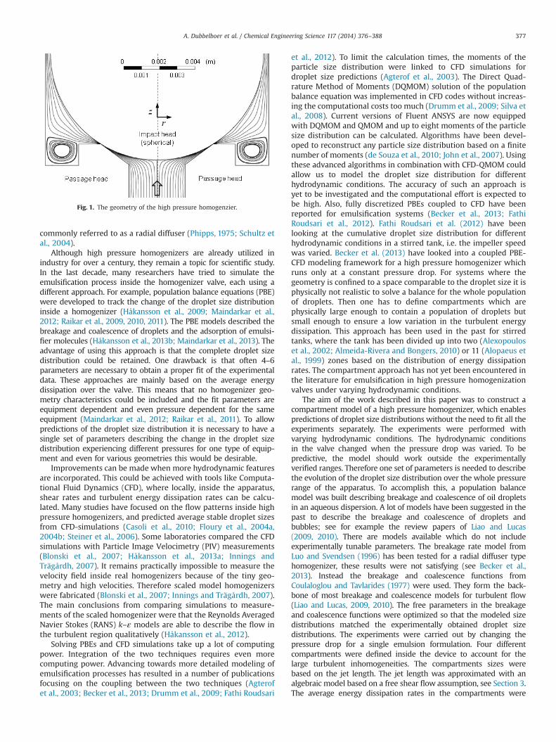
the droplet size during the production process. A typical produc-tion process consists of two steps: in the first step oil and waterphases are mixed, possibly with other ingredients, forming acoarse emulsion; then, in the second step the droplet size ofthe dispersed phase is further reduced to a desired value.High pressure homogenization valves are often applied in thesecond step where they are able to generate submicron dropletsizes (Karbstein and Schubert, 1995; Schultz et al., 2004). A highpressure homogenizer consists of a pump and a homogenizingnozzle (Schuchmann and Schubert, 2001). The coarse emulsion isentering from the bottom along the main axis. The emulsion hitsa solid impact head and spreads out through the narrow gap inthe radial direction (Fig. 1). This type of homogenizing valve is

Contents lists available at ScienceDirect

journal homepage: www.elsevier.com/locate/ces

Chemical Engineering Science

http://dx.doi.org/10.1016/j.ces.2014.06.0470009-2509/& 2014 Elsevier Ltd. All rights reserved.

n Corresponding author. Tel.: þ31 40 247 2328.E-mail address: j.meuldijk@tue.nl (J. Meuldijk).

Chemical Engineering Science 117 (2014) 376–388

commonly referred to as a radial diffuser (Phipps, 1975; Schultz etal., 2004).

Although high pressure homogenizers are already utilized inindustry for over a century, they remain a topic for scientific study.In the last decade, many researchers have tried to simulate theemulsification process inside the homogenizer valve, each using adifferent approach. For example, population balance equations (PBE)were developed to track the change of the droplet size distributioninside a homogenizer (Håkansson et al., 2009; Maindarkar et al.,2012; Raikar et al., 2009, 2010, 2011). The PBE models described thebreakage and coalescence of droplets and the adsorption of emulsi-fier molecules (Håkansson et al., 2013b; Maindarkar et al., 2013). Theadvantage of using this approach is that the complete droplet sizedistribution could be retained. One drawback is that often 4–6parameters are necessary to obtain a proper fit of the experimentaldata. These approaches are mainly based on the average energydissipation over the valve. This means that no homogenizer geo-metry characteristics could be included and the fit parameters areequipment dependent and even pressure dependent for the sameequipment (Maindarkar et al., 2012; Raikar et al., 2011). To allowpredictions of the droplet size distribution it is necessary to have asingle set of parameters describing the change in the droplet sizedistribution experiencing different pressures for one type of equip-ment and even for various geometries this would be desirable.

Improvements can be made when more hydrodynamic featuresare incorporated. This could be achieved with tools like Computa-tional Fluid Dynamics (CFD), where locally, inside the apparatus,shear rates and turbulent energy dissipation rates can be calcu-lated. Many studies have focused on the flow patterns inside highpressure homogenizers, and predicted average stable droplet sizesfrom CFD-simulations (Casoli et al., 2010; Floury et al., 2004a,2004b; Steiner et al., 2006). Some laboratories compared the CFDsimulations with Particle Image Velocimetry (PIV) measurements(Blonski et al., 2007; Håkansson et al., 2013a; Innings andTrägårdh, 2007). It remains practically impossible to measure thevelocity field inside real homogenizers because of the tiny geo-metry and high velocities. Therefore scaled model homogenizerswere fabricated (Blonski et al., 2007; Innings and Trägårdh, 2007).The main conclusions from comparing simulations to measure-ments of the scaled homogenizer were that the Reynolds AveragedNavier Stokes (RANS) k–ε models are able to describe the flow inthe turbulent region qualitatively (Håkansson et al., 2012).

Solving PBEs and CFD simulations take up a lot of computingpower. Integration of the two techniques requires even morecomputing power. Advancing towards more detailed modeling ofemulsification processes has resulted in a number of publicationsfocusing on the coupling between the two techniques (Agterofet al., 2003; Becker et al., 2013; Drumm et al., 2009; Fathi Roudsari

et al., 2012). To limit the calculation times, the moments of theparticle size distribution were linked to CFD simulations fordroplet size predictions (Agterof et al., 2003). The Direct Quad-rature Method of Moments (DQMOM) solution of the populationbalance equation was implemented in CFD codes without increas-ing the computational costs too much (Drumm et al., 2009; Silva etal., 2008). Current versions of Fluent ANSYS are now equippedwith DQMOM and QMOM and up to eight moments of the particlesize distribution can be calculated. Algorithms have been devel-oped to reconstruct any particle size distribution based on a finitenumber of moments (de Souza et al., 2010; John et al., 2007). Usingthese advanced algorithms in combination with CFD-QMOM couldallow us to model the droplet size distribution for differenthydrodynamic conditions. The accuracy of such an approach isyet to be investigated and the computational effort is expected tobe high. Also, fully discretized PBEs coupled to CFD have beenreported for emulsification systems (Becker et al., 2013; FathiRoudsari et al., 2012). Fathi Roudsari et al. (2012) have beenlooking at the cumulative droplet size distribution for differenthydrodynamic conditions in a stirred tank, i.e. the impeller speedwas varied. Becker et al. (2013) have looked into a coupled PBE-CFD modeling framework for a high pressure homogenizer whichruns only at a constant pressure drop. For systems where thegeometry is confined to a space comparable to the droplet size it isphysically not realistic to solve a balance for the whole populationof droplets. Then one has to define compartments which arephysically large enough to contain a population of droplets butsmall enough to ensure a low variation in the turbulent energydissipation. This approach has been used in the past for stirredtanks, where the tank has been divided up into two (Alexopouloset al., 2002; Almeida-Rivera and Bongers, 2010) or 11 (Alopaeus etal., 1999) zones based on the distribution of energy dissipationrates. The compartment approach has not yet been encountered inthe literature for emulsification in high pressure homogenizationvalves under varying hydrodynamic conditions.

The aim of the work described in this paper was to construct acompartment model of a high pressure homogenizer, which enablespredictions of droplet size distributions without the need to fit all theexperiments separately. The experiments were performed withvarying hydrodynamic conditions. The hydrodynamic conditionsin the valve changed when the pressure drop was varied. To bepredictive, the model should work outside the experimentallyverified ranges. Therefore one set of parameters is needed to describethe evolution of the droplet size distribution over the whole pressurerange of the apparatus. To accomplish this, a population balancemodel was built describing breakage and coalescence of oil dropletsin an aqueous dispersion. A lot of models have been suggested in thepast to describe the breakage and coalescence of droplets andbubbles; see for example the review papers of Liao and Lucas(2009, 2010). There are models available which do not includeexperimentally tunable parameters. The breakage rate model fromLuo and Svendsen (1996) has been tested for a radial diffuser typehomogenizer, these results were not satisfying (see Becker et al.,2013). Instead the breakage and coalescence functions fromCoulaloglou and Tavlarides (1977) were used. They form the back-bone of most breakage and coalescence models for turbulent flow(Liao and Lucas, 2009, 2010). The free parameters in the breakageand coalescence functions were optimized so that the modeled sizedistributions matched the experimentally obtained droplet sizedistributions. The experiments were carried out by changing thepressure drop for a single emulsion formulation. Four differentcompartments were defined inside the device to account for thelarge turbulent inhomogeneities. The compartments sizes werebased on the jet length. The jet length was approximated with analgebraic model based on a free shear flow assumption, see Section 3.The average energy dissipation rates in the compartments were

Fig. 1. The geometry of the high pressure homogenzier.

A. Dubbelboer et al. / Chemical Engineering Science 117 (2014) 376–388 377

estimated with a k–ε turbulent model. Then the energy dissipationrates were fed to the breakage and coalescence kernels of thepopulation balance model. The performance of a four compartmentmodel was compared to that of a single compartment model and atwo compartment model.

2. Experimental methods

To generate a pre-emulsion for homogenization, 1 wt% ofPluronic F68 emulsifying agent (Sigma Aldrich) was dissolved inNanopure demineralized water. Subsequently 10 wt% of sunfloweroil was slowly added while stirring with a Silverson L5T mixer. TheSilverson mixer was equipped with a General Purpose Disintegrat-ing Head and a Standard Emulsor Screen. The mixture was stirredfor 5 min at 6000 rpm, the resulting d32 and dv99 were 15 and54 μm, respectively. The droplet size distributions of all sampleswere measured with a static light scattering device (MalvernMastersizer 2000). The viscosities of the sunflower oil and thePluronic F68 solution were 50 and 1.3 mPa s, respectively. Theywere measured with a rotational shear rheometer (2000EX,TA Instruments) at a constant temperature of 25 1C. The equili-brium surface tension was carefully determined by Maindarkaret al. (2013) for a vegetable oil in water emulsion stabilized byPluronic F68. At 25 1C and with a Pluronic concentration of1.3 mol/m3 the surface tension is 17 mN/m.

For homogenization a lab scale Niro Soavi high pressure homo-genizer was used (type: Panda NS1001L). It was operated with areciprocating multi-plunger pump. The homogenizer had a constantthroughput of 13 l/h. A manual valve controlled the pressure drop. Thepressure was varied between 200 and 800 bar. The pressure remainedconstant within þ20 and �20 bar of the target pressure. The coarseemulsion was passed several times through the high pressure homo-genizer. The reproducibility of the experiments was checked byrepeating the homogenization experiments at 200 and 800 bar(Fig. 2a and b). The differences in the measured droplet size distribu-tions were quantified using an objective function (Ψ), see Eq. (28) andalso Maindarkar et al. (2012) and Raikar et al. (2009). In theoptimization of the free parameters the modeled droplet size distribu-tions are therefore converged when Ψr0.006. All experiments wereperformed with the same coarse emulsion.

3. Compartment sizing

In a previous contribution it was already shown that for thistype of homogenizer breakup is likely to happen in the jet leavingthe narrow restriction (Dubbelboer et al., 2013). This was found forother similar types of homogenizers as well (Innings and Trägårdh,

2007). Therefore the compartments need to be defined in the jetarea. The height of the compartments is restricted by the valveimpact and passage heads. Only the length of the compartments inthe radial direction must be estimated and this is based on the jetlength. The jet is spreading in a radial direction and is expected todie out sooner than, for example, a planar jet for which algebraicequations are readily available in most textbooks. Algebraicequations for the planar and round jets are surprisingly accuratewhen compared to experiments. The flows in planar and roundjets are the so-called free shear flows, where there is no influenceof solid boundaries above or below the jet. Then it appears that themomentum in the jet is conserved and the spreading rate isconstant. In fact, the spreading angle of the jet for both geometrieswas found to be around 121. When the jet was assumed to be ofthe free-shear-flow type the radial spreading of the jet can bedescribed by

u0

U0¼ 1þα

2r2�r20r0δ0

� �� ��1=2

ð1Þ

In which ū0 is the average center line jet speed, U0 is the center linejet speed at r0, δ0 is the jet width at r0, α is the entrainmentcoefficient and r0 is the point where the jet becomes self-similar.Because planar and round jets both have an entrainment coeffi-cient of 0.42 the same entrainment coefficient was assumed forthe radial jet. The distance the jet spreads in the radial directioncan now be estimated with Eq. (1). The starting jet width is takenequal to the spatial distance between the passage and impact

Fig. 2. The inlet (gray line), outlet (black line) and repeated outlet (black dashed line) droplet size distributions measured with a static light scattering device; left, after1 pass at 200 bar with Ψ¼0.0057 and right, after 1 pass at 800 bar with Ψ¼0.0060.

Fig. 3. The region between the impact and passage head directly after the gap withthe 4 compartments, the boundaries between the compartments are designated asa, b and c.

A. Dubbelboer et al. / Chemical Engineering Science 117 (2014) 376–388378

head. These gap heights were estimated by Dubbelboer et al.(2013). For a decay of 90%, with r0 is 2.5 mm and δ0 is 0.0016 mm,the jet reaches to 2.9 mm in the radial direction. The singlecompartment model has a compartment which reaches from r0to r. A two compartment model was made which contained twocompartments divided equally over the distance r–r0. Likewise thefour compartment model has four compartments divided equallyover the distance r–r0, see Fig. 3. The resulting compartmentvolumes and residence times of the four compartments are givenin Table 1. The residence time in a compartment should besufficient for droplet breakup to occur. This will be checked byanalyzing the time scales for turbulence and droplet deformationin Section 5.

The compartments are placed in series where the outlet ofcompartment one was the inlet for compartment two and so forth.A population balance was solved for every compartment. The firstrequirement for the application of the PBE method is that thecontrol volume must be large enough to contain a population ofparticles. There are no clear criteria available, but here the numberof particles in compartment one becomes ϕV1/(πd323 /6)�106,which is believed to be sufficiently large for the use of populationbalance methods in this tiny geometry. Now that the compart-ments are defined the hydrodynamic forces inside the compart-ments must be determined. The hydrodynamic pressure forexample is responsible for droplet fragmentation and is relatedto the energy dissipation. The turbulent energy dissipation in eachcompartment was estimated using the infamous k–ε model.

4. Computational Fluid Dynamics

High velocity jets have turbulent characteristics; thereforea turbulence modeling approach has to be adopted. The firstassumption made was the single phase approximation. It wasassumed that the dispersed oil droplets move with the same speedas the continuous phase. Therefore the emulsion was modeled as aquasi single phase with an average density and an average New-tonian viscosity. Then, the ensemble averaged velocity field of theturbulent jet was simulated using the Reynolds Averaged NavierStokes (RANS) equation. In principle this time averaged equation istime independent. Hence the steady state RANS equation forincompressible and isothermal flow reads

ρ ~u U∇ui ¼ � ∂p∂xi

þ ∂∂xi

½τijþτRij� ð2Þ

The over-bar represents an averaged quantity, the apostrophe thefluctuation from the average and the bold faced symbols representvectors. Further, ρ is the fluid density, u is the fluid velocity, p isthe pressure, x is the spatial coordinate, τij are the stresses actingon the fluid and τijR are the Reynolds stresses. The Reynoldsaveraged continuity equation gives

∇Uu¼ 0 ð3Þ

The RANS equations with the Reynolds averaged continuityequation leave six degrees of freedom, the so-called Reynolds

stresses.

τRij ¼ ρ

u021 u0

1u02 u0

1u03

u02u

01 u02

2 u02u

03

u03u

01 u0

3u02 u02

3

0BBB@

1CCCA ð4Þ

A method is needed to close the set of equations. Single-pointclosure models are relatively easy to implement and widely usedin engineering. The Boussinesq hypothesis relates the Reynoldsstresses to the mean strain rates via

�u0iu

0j ¼ 2νtSij�

23kδij ð5Þ

Here, δij is the Kronecker delta, Sij is the rate of strain tensor, k isthe kinetic turbulent energy and νt is the eddy viscosity. Now theproblem is shifted to finding the eddy viscosity at each point in theflow. In the k–ε model the eddy viscosity scales as follows:

νt ¼ Cμk2

εð6Þ

In which ε is the turbulent energy dissipation and Cμ is adimensionless constant. The transport equation for turbulentkinetic energy reads

uU∇k¼ νþ νtσk

� �ΔkþðτRij=ρÞSij�ε ð7Þ

And for turbulent energy dissipation

uU∇ε¼ νþ νtσε

� �ΔεþC1

εkðτRij=ρÞSij�C2

ε2

kð8Þ

In which ν is the kinematic viscosity of the liquid. In the transportequations for k and ε appear the following dimensionless para-meters: σk, σε, C1 and C2. The set of equations described here forma closed and solvable set of equations. The derivation of allequations can be found in any textbook (see e.g. Davidson, 2006,Chapter 4). In the k–ε models, there are only two parameterswhich characterize the turbulence. It is a simple model neglectingmany details of the turbulent flow. Because the interest lies in theaverage energy dissipation inside a relatively large compartmentthere is no need to resolve the finer turbulence characteristics ofthe flow.

The k–ε model is the most frequently used engineering modelof turbulence. It has proven to be reliable for simple shear flowsbut fails in complex configurations, high anisotropic turbulenceand close to solid surfaces (Davidson, 2006, Chapter 4). There aremany variations of the k–ε model with each having their ownlimitations which are well documented nowadays. The standardk–ε model and two of its more refined extensions (termedRealizable and RNG k–ε models) were experimentally validatedfor a scaled high pressure homogenizer using 2D Particle ImageVelocimetry (PIV) (see Håkansson et al., 2011, 2012). The refinedk–ε models give better estimates for the turbulent kinetic energyinside the narrow restriction. In the jet region the RNG modelgives a slightly better prediction of the production of turbulentkinetic energy than its Realizable counterpart but is not welldescribed by either model.

The RNG k–ε model was derived using a statistical techniquecalled Re-Normalization Group theory. The RNG approach derivedthe transport equations for k and ε in a slightly different manner.The result is a different expression for the generation of turbulentkinetic energy from the mean velocity gradients. The transportequation for turbulent energy dissipation obtains the followingadditional parameters:

C2 ¼ Cn

2þCμs3ð1�s=s0Þ

1þβs3ð9Þ

Table 1The compartment volumes and mean residence times.

Compartment V/m3 tres/s

1 8.9E�12 2.4E�062 2.6E�11 7.1E�063 4.4E�11 1.2E�054 6.3E�11 1.7E�05

A. Dubbelboer et al. / Chemical Engineering Science 117 (2014) 376–388 379

with

s¼ffiffiffiffiffiffiffiffiffiffiffiffi2SijSij

q kε

ð10Þ

Effectively this means that in areas of large strain (s4s0) there isless dissipation of ε, a reduction of k and overall lower estimates ofthe eddy viscosity. Moreover, all constants are derived analyticallywith the RNG procedure, with the exception of β which needs tobe fitted from experiment. The value of β¼0.012 has been foundin the past and was taken as such. For the rest of the constants:Cμ¼0.0845, σk¼0.7194, σε¼0.7194, C1¼1.42, C2n¼1.68 ands0¼4.38. The RNG k–ε model is standard implemented in mostCFD software packages with these default values.

4.1. Boundary conditions and numerical methods

The boundary conditions for the RANS equation at the homo-genizer inlet was the velocity determined from the flow rate andat the outlet the gauge pressure was set to zero. At the walls theno-slip condition was applied. The velocity pressure coupling wassolved numerically with the SIMPLE scheme and second orderupwind discretization was used for all transport equations. The k–ε transport equations also need boundary conditions. At the inletthe flow is not turbulent; hence the kinetic turbulent energy andthe turbulent energy dissipation were set to zero at the inlet. Theturbulence modeling close to the walls needs some special atten-tion and will be dealt with in the next section.

4.2. Modeling close to the wall and grid building

The remaining problem is the behavior of the k–ε model closeto the solid boundaries. Near wall behavior of k–ε models is wellknown to give erroneous results (see e.g. Durbin and Pettersson-Reif, 2001, Chapter 6). Approaching the solid boundaries theviscous stresses outpace the inertial stresses. The fluid layer closeto the wall where the viscous stresses cannot be neglected any-more is called the logarithmic layer. Therefore the k–ε equationsare usually abandoned in the logarithmic layer. Instead, so-calledwall functions for the production and dissipation of k are imple-mented. The boundary conditions for the k–ε model are thenimposed on top of the logarithmic layer; however, in practice theboundary conditions are applied to the first grid point adjacent tothe wall. Then, it is a necessary requirement for the first grid pointto be located at the logarithmic layer. The first grid point must belocated at a dimensionless normal distance to the wall of yþ�15(ANSYSs Fluent, 2011, 14.0, help system, 4.13, ANSYS, Inc.). The

distance normal to the wall is made dimensionless as follows:

yþ ¼ffiffiffiffiffiffiffiffiffiffiffiτw=ρ

pν

y ð11Þ

In which τw is the stress at the wall and y is the actual distancenormal to the wall. Wall functions will give inaccurate results for agrid with yþo15. In that situation a two layer zonal model willbe more appropriate. In the two layer zonal model the momentumand turbulent kinetic energy equations are retained for bothzones, since the turbulent kinetic energy is zero at the wallsbecause of the no-slip condition. Only the ε transport equation isreplaced by a mixing length transport equation in the zoneadjacent to the wall, making this model also suitable for separatingflows (recirculation) (Chen and Patel, 1988). In Fig. 4 two types ofwall treatment are analyzed at the edges of the four compartmentsperpendicular to the flow.

The viscosity dominated region close to the walls should berelatively large because of the moderate Reynolds numbers. TheReynolds number in the channel and at the start of the jet, basedon the channel height, is �200. At these moderate Reynoldsnumbers no turbulence is generally expected for plane channelflow. Also at low Reynolds numbers the yþ values remain fairlysmall for a coarse grid. In the high pressure homogenizer the mostenergy dissipation is expected to be in the center of the turbulentjet, which is observed with the two-layer zonal model, see Fig. 3.The standard wall function model over predicts the turbulentenergy dissipation in close proximity of the boundary even atyþ¼14. It appears that the two-layer zonal model gives the mostphysically reasonable results for the energy dissipation close tothe walls.

From the discussion above the grid appears to be coarsefor yþo15, and then it follows that the two-layer zonal modelis the preferred model. From a practical point of view a grid with alow resolution is preferred. Convergence of finer meshes waschecked with respect to mass conservation and the quantity ofinterest: the average energy dissipation inside the compartments.Three meshes were constructed with a low, medium and highresolution. The three grids are compared in Table 2. A second-order upwind discretization scheme was used for the transportequations of momentum, turbulent kinetic energy (k) and turbu-lent dissipation rate (ε).

The difference between the mass flow rate at the in- and outletwas well below 1% for all meshes. The turbulent energy dissipationconverged only for the meshes with a medium and high resolu-tion. This difference in the integrated energy dissipation overthe compartment volumes between the finer meshes was �5%.

Fig. 4. The modeled turbulent energy dissipation at the edges of the compartments perpendicular to the flow; on the left the wall function model on the right the two-layerzonal model for yþ¼14; (●): boundary a, (þ): boundary b and (▲): boundary c (see Fig. 3 for the boundaries).

A. Dubbelboer et al. / Chemical Engineering Science 117 (2014) 376–388380

For that reason the grid with the medium mesh resolution wasselected to best fit the needs of this research.

4.3. CFD results

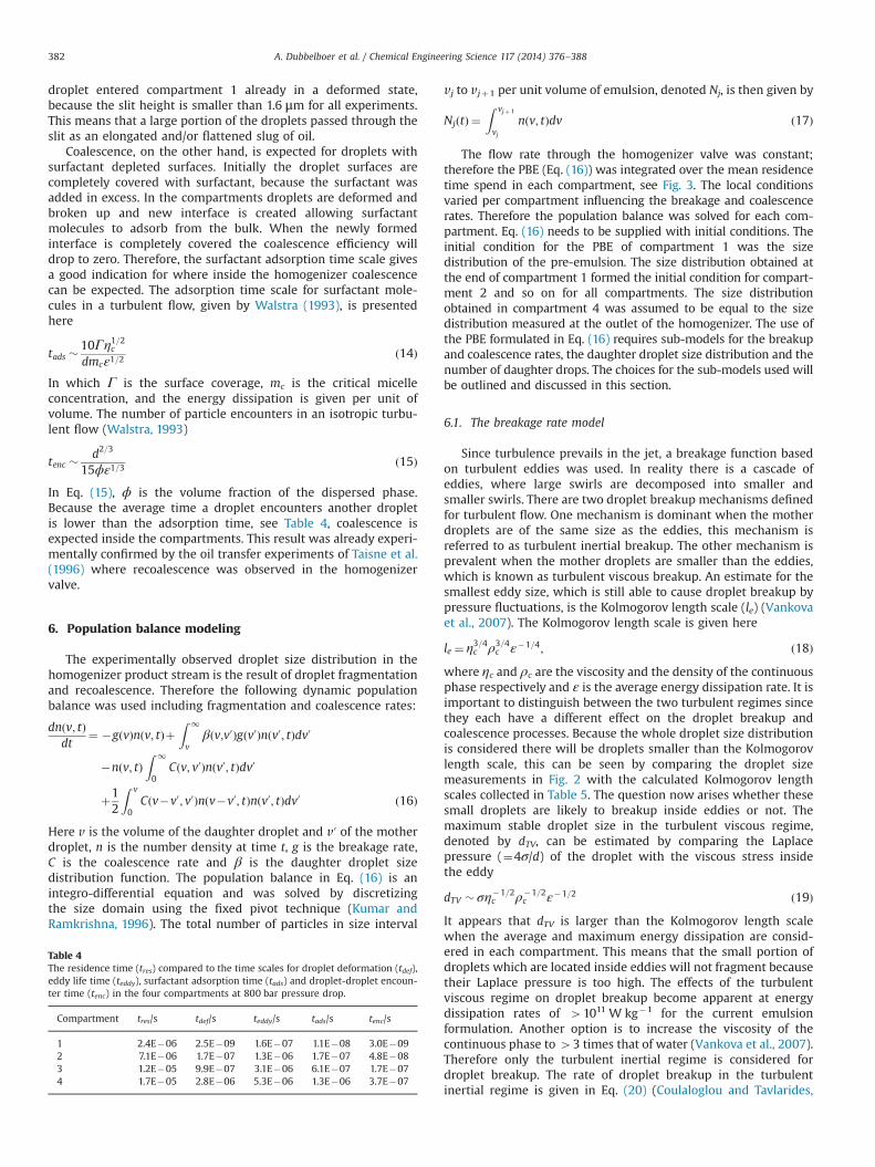
A Computational Fluid Dynamics (CFD) simulation was per-formed to estimate the local turbulent energy dissipation rates.The results of the CFD simulation are discussed here. The stream-lines visualize the direction in which the emulsion travels throughthe homogenizer valve (Fig. 1). The emulsion flows around theimpact head and leaves at the top. A vortex is formed in the cornerof the passage head and the impact ring. The active part of the jetdid not reach the vortex. No significant differences in the flowprofiles were observed when changing the position of the valve tomodify the pressure drop, results not shown.

The turbulent energy dissipation, which was correlated todroplet breakup, is displayed for the different parts of the homo-genizer in a contour plot (Fig. 5). The largest energy dissipationwas found directly after the narrow restriction. It was here wherethe droplet breakup was anticipated. The average and maximumof the turbulent energy dissipation are given in Table 3. Theaverage energy dissipation per compartment was the highestdirectly after the gap and decreased exponentially with distancefrom the gap. The spread in the energy dissipation was also thehighest in the first compartment (Table 3). In compartment 1 theaverage energy dissipation increases with increasing pressuredrop. For the other three compartments, however, the averageenergy dissipation was slightly decreasing with pressure drop(Fig. 6). For now it is not certain whether this is caused by the CFDor this is actual physics.

5. Time scale analysis

In this section the time scales for several physical processesinvolving emulsification are discussed and compared to theresidence times of the compartments which were defined inSection 3. The residence time (tres) should be sufficiently long todeform the droplets. The droplets are deformed by eddies ofapproximately the same size. Therefore the eddy life time (teddy)should be of the same order as the deformation time or longer i.e.

tresZteddyZtdef. The residence time was compared to the timescales for droplet deformation and the eddy life time for a dropletof 10 μm in diameter (Table 3). Estimations for both times scalesare given by Eqs. (12) and (13) (Walstra, 1993).

tdef �ηd

5ρcε2=3d2=3; ð12Þ

where ηd is the dynamic viscosity of the dispersed phase, ρc is thecontinuous phase density, ε is the average energy dissipation(W kg�1) and d is the droplet diameter. The eddy life time isbased on an eddy with the same size as the mother droplet:

teddy �d2=3

ε1=3ð13Þ

Both time scales were calculated using the average energydissipation in each compartment. The residence time in the fourcompartments was enough for eddies to appear and to disappear.The eddy life time in each compartment was sufficient to deform adroplet of 10 μm in diameter. It should be noted that a 10 μm

Table 2Grid comparison.

Gridresolution

Number of cells along compartmentborder

Total number ofcells

yþ

Low 12 24,995 14Medium 35 37,806 5High 50 54,366 3

Fig. 5. The contours of the logarithm of the turbulent energy dissipation, the region directly after the narrow restriction is magnified and the four compartments can be seen.

Table 3Results extracted from the CFD-simulation (800 bar pressure drop): the average ðεÞand maximum (εmax) turbulent energy dissipation for the four compartments.

Compartment ε/W kg�1 εmax/W kg�1

1 2.6Eþ10 3.3Eþ112 4.4Eþ07 2.9Eþ083 3.2Eþ06 1.1Eþ074 6.6Eþ05 1.6Eþ06

Fig. 6. The average energy dissipation as a function of pressure drop for the fourcompartments; (♦): compartment 1, (■): compartment 2, (▲): compartment 3 and(� ): compartment 4.

A. Dubbelboer et al. / Chemical Engineering Science 117 (2014) 376–388 381

droplet entered compartment 1 already in a deformed state,because the slit height is smaller than 1.6 μm for all experiments.This means that a large portion of the droplets passed through theslit as an elongated and/or flattened slug of oil.

Coalescence, on the other hand, is expected for droplets withsurfactant depleted surfaces. Initially the droplet surfaces arecompletely covered with surfactant, because the surfactant wasadded in excess. In the compartments droplets are deformed andbroken up and new interface is created allowing surfactantmolecules to adsorb from the bulk. When the newly formedinterface is completely covered the coalescence efficiency willdrop to zero. Therefore, the surfactant adsorption time scale givesa good indication for where inside the homogenizer coalescencecan be expected. The adsorption time scale for surfactant mole-cules in a turbulent flow, given by Walstra (1993), is presentedhere

tads �10Γη1=2c

dmcε1=2ð14Þ

In which Γ is the surface coverage, mc is the critical micelleconcentration, and the energy dissipation is given per unit ofvolume. The number of particle encounters in an isotropic turbu-lent flow (Walstra, 1993)

tenc � d2=3

15ϕε1=3ð15Þ

In Eq. (15), ϕ is the volume fraction of the dispersed phase.Because the average time a droplet encounters another dropletis lower than the adsorption time, see Table 4, coalescence isexpected inside the compartments. This result was already experi-mentally confirmed by the oil transfer experiments of Taisne et al.(1996) where recoalescence was observed in the homogenizervalve.

6. Population balance modeling

The experimentally observed droplet size distribution in thehomogenizer product stream is the result of droplet fragmentationand recoalescence. Therefore the following dynamic populationbalance was used including fragmentation and coalescence rates:

dnðv; tÞdt

¼ �gðvÞnðv; tÞþZ 1

vβðv;v0Þgðv0Þnðv0; tÞdv0

�nðv; tÞZ 1

0Cðv; v0Þnðv0; tÞdv0

þ12

Z v

0Cðv�v0; v0Þnðv�v0; tÞnðv0; tÞdv0 ð16Þ

Here v is the volume of the daughter droplet and v0 of the motherdroplet, n is the number density at time t, g is the breakage rate,C is the coalescence rate and β is the daughter droplet sizedistribution function. The population balance in Eq. (16) is anintegro-differential equation and was solved by discretizingthe size domain using the fixed pivot technique (Kumar andRamkrishna, 1996). The total number of particles in size interval

vj to vjþ1 per unit volume of emulsion, denoted Nj, is then given by

NjðtÞ ¼Z vjþ 1

vjnðv; tÞdv ð17Þ

The flow rate through the homogenizer valve was constant;therefore the PBE (Eq. (16)) was integrated over the mean residencetime spend in each compartment, see Fig. 3. The local conditionsvaried per compartment influencing the breakage and coalescencerates. Therefore the population balance was solved for each com-partment. Eq. (16) needs to be supplied with initial conditions. Theinitial condition for the PBE of compartment 1 was the sizedistribution of the pre-emulsion. The size distribution obtained atthe end of compartment 1 formed the initial condition for compart-ment 2 and so on for all compartments. The size distributionobtained in compartment 4 was assumed to be equal to the sizedistribution measured at the outlet of the homogenizer. The use ofthe PBE formulated in Eq. (16) requires sub-models for the breakupand coalescence rates, the daughter droplet size distribution and thenumber of daughter drops. The choices for the sub-models used willbe outlined and discussed in this section.

6.1. The breakage rate model

Since turbulence prevails in the jet, a breakage function basedon turbulent eddies was used. In reality there is a cascade ofeddies, where large swirls are decomposed into smaller andsmaller swirls. There are two droplet breakup mechanisms definedfor turbulent flow. One mechanism is dominant when the motherdroplets are of the same size as the eddies, this mechanism isreferred to as turbulent inertial breakup. The other mechanism isprevalent when the mother droplets are smaller than the eddies,which is known as turbulent viscous breakup. An estimate for thesmallest eddy size, which is still able to cause droplet breakup bypressure fluctuations, is the Kolmogorov length scale (le) (Vankovaet al., 2007). The Kolmogorov length scale is given here

le ¼ η3=4c ρ3=4c ε�1=4; ð18Þ

where ηc and ρc are the viscosity and the density of the continuousphase respectively and ε is the average energy dissipation rate. It isimportant to distinguish between the two turbulent regimes sincethey each have a different effect on the droplet breakup andcoalescence processes. Because the whole droplet size distributionis considered there will be droplets smaller than the Kolmogorovlength scale, this can be seen by comparing the droplet sizemeasurements in Fig. 2 with the calculated Kolmogorov lengthscales collected in Table 5. The question now arises whether thesesmall droplets are likely to breakup inside eddies or not. Themaximum stable droplet size in the turbulent viscous regime,denoted by dTV, can be estimated by comparing the Laplacepressure (¼4σ/d) of the droplet with the viscous stress insidethe eddy

dTV � ση�1=2c ρ�1=2

c ε�1=2 ð19ÞIt appears that dTV is larger than the Kolmogorov length scalewhen the average and maximum energy dissipation are consid-ered in each compartment. This means that the small portion ofdroplets which are located inside eddies will not fragment becausetheir Laplace pressure is too high. The effects of the turbulentviscous regime on droplet breakup become apparent at energydissipation rates of 41011 W kg�1 for the current emulsionformulation. Another option is to increase the viscosity of thecontinuous phase to 43 times that of water (Vankova et al., 2007).Therefore only the turbulent inertial regime is considered fordroplet breakup. The rate of droplet breakup in the turbulentinertial regime is given in Eq. (20) (Coulaloglou and Tavlarides,

Table 4The residence time (tres) compared to the time scales for droplet deformation (tdef),eddy life time (teddy), surfactant adsorption time (tads) and droplet-droplet encoun-ter time (tenc) in the four compartments at 800 bar pressure drop.

Compartment tres/s tdef/s teddy/s tads/s tenc/s

1 2.4E�06 2.5E�09 1.6E�07 1.1E�08 3.0E�092 7.1E�06 1.7E�07 1.3E�06 1.7E�07 4.8E�083 1.2E�05 9.9E�07 3.1E�06 6.1E�07 1.7E�074 1.7E�05 2.8E�06 5.3E�06 1.3E�06 3.7E�07

A. Dubbelboer et al. / Chemical Engineering Science 117 (2014) 376–388382

1977):

gðvÞ ¼ K1v�2=9ε1=3

ð1þϕÞ exp �K2σð1þϕÞ2ρdv5=9ε

2=3

!; ð20Þ

where K1 and K2 are adjustable dimensionless parameters, σ is theinterfacial tension and ρd is dispersed phase density. Eq. (20) is acombination of the breakage frequency and the breakage prob-ability (the exponential term). The breakage frequency is increas-ing for smaller droplets. The breakage probability is approximatelyequal to one for all droplet sizes larger than the maximum stabledroplet size. The factor 1/(1þϕ) accounts for damping of turbu-lence by the dispersed phase (Coulaloglou and Tavlarides, 1977).

6.2. The daughter droplet size distribution function

From single droplet experiments a lot can be learned aboutthe breakup behavior of droplets with respect to the number offragments and the sizes of the daughter droplets. Andersson andAndersson (2006) observed single droplet breakup with a highspeed camera and concluded that equal sized breakup is themost probable. In this work the daughter droplet size distributionfunction was assumed to be a uniform probability function, mean-ing that the droplets obtained after a breakage event have thesame size. The uniform daughter droplet size distribution functionfor multiple breakup was derived by (Hill and Ng, 1996)

βðv; v0Þ ¼ pðp�1Þ 1� vv0

� �p�2; ð21Þ

where p is the number of daughter droplets. In turbulent flowsviscous droplets were shown to stretch to long threads, up to 20times the initial droplet diameter (Andersson and Andersson,2006). The thread diameter then becomes �0.18d, based on theconservation of volume. The breakup of liquid viscous threads iscaused by small disturbances present on the interface which growand disintegrate the liquid cylinder because the interfacial tensiontends to minimize the interfacial area between two phases.The fragment size depends on the viscosity ratio for liquid threadbreakup. For the current formulation, the daughter droplet sizebecomes 3.2 times the thread diameter, using the analysisof Janssen and Meijer (1995), which results into five daughterdroplets.

6.3. The coalescence rate model

The coalescence rate is modeled as the product of the collisionfrequency h(v, v0) and the coalescence efficiency Λ(v, v0), since notall collisions lead to coalescence, especially not when a surfaceactive component is present. The coalescence rate reads

Cðv; v0Þ ¼ hðv; v0ÞΛðv; v0Þ ð22Þ

Coulaloglou and Tavlarides (1977) proposed to use the kinetictheory of gasses to derive the turbulent random motion-inducedcollision frequency between droplets of size v and v0, which is

given here

hðv;v0Þ ¼ K3ε1=3

ð1þϕÞðv2=3þv02=3Þðv2=9þv02=9Þ1=2 ð23Þ

In which K3 is a dimensionless adjustable parameter and the factor1/(1þϕ) accounts, likewise, for the damping of turbulence by thedispersed phase. Eq. (23) is often encountered in the literature todescribe the collision frequency. Although more comprehensivemodels exist, for example which take the eddy size into account,the goal is not to make the modeling exercise too elaborate. Moreadvanced models can be found in a recent review paper publishedby Liao and Lucas (2010).

The coalescence efficiency is based on the film drainage model,which is also one of the most frequently applied models forcoalescence efficiency (Liao and Lucas, 2010). The efficiency isone when the contact time between droplets is greater than thefilm drainage time. The coalescence efficiency then reads

Λðv;v0Þ ¼ exp � tdraintcontact

� �: ð24Þ

The drainage time is the time required for the liquid film todrain from between the droplets. For deformable particles withimmobile interfaces, Coulaloglou and Tavlarides (1977) estimatedthe drainage time as

tdrain �ηcρcε2=3ðvþv0Þ2=9

σ2

1

h2� 1

h20

!v1=3v01=3

v1=3þv01=3

� �4

ð25Þ

In which h and h0 are the critical and initial film thickness; theyare replaced by a fit parameter. The approximation of immo-bility of the film surface is applicable to systems with a highviscosity ratio and/or surfactant dissolved in the continuous phase(Chesters, 1991). Coulaloglou and Tavlarides (1977) estimated thecontact time by a dimensional analysis from Levich (1962)

tcontact �ðvþv0Þ2=9ε1=3

ð26Þ

The coalescence rate becomes

Cðv;v0Þ ¼ K3ε1=3

ð1þϕÞðv2=3þv02=3Þðv2=9þv02=9Þ

�exp �K4ηcρcε

σ2 1þϕ� �3 v1=3v01=3

v1=3þv01=3

� �4 !: ð27Þ

6.4. Parameter optimization

The free parameters (K1 up to K4) can be obtained by comparingthe model with the experimental results via a least squaresoptimization. Parameters K1–3 were expected to be of the orderunity because of the derivation of the model equations. ParameterK4, however, was anticipated to be a large number because theterm with the film thickness (see Eq. (25)) was clustered togetherwith the empirical constant, K4. The parameters K1 up to K4 of thebreakage and coalescence rates were found by minimizing thefollowing objective function:

Ψ ¼∑M

j ðn½j�exp�ϕjÞ2

∑Mj ðn

½j�expÞ2

; ð28Þ

here M is the number of discrete size classes, nexp is the measuredvolume fraction of droplets in size class j and ϕj is the volumefraction of droplets in size class j. The volume fraction of dropletsin size class j was calculated from the discreet average number ofdroplets in size class j, by using

ϕj ¼Njvjϕ

ð29Þ

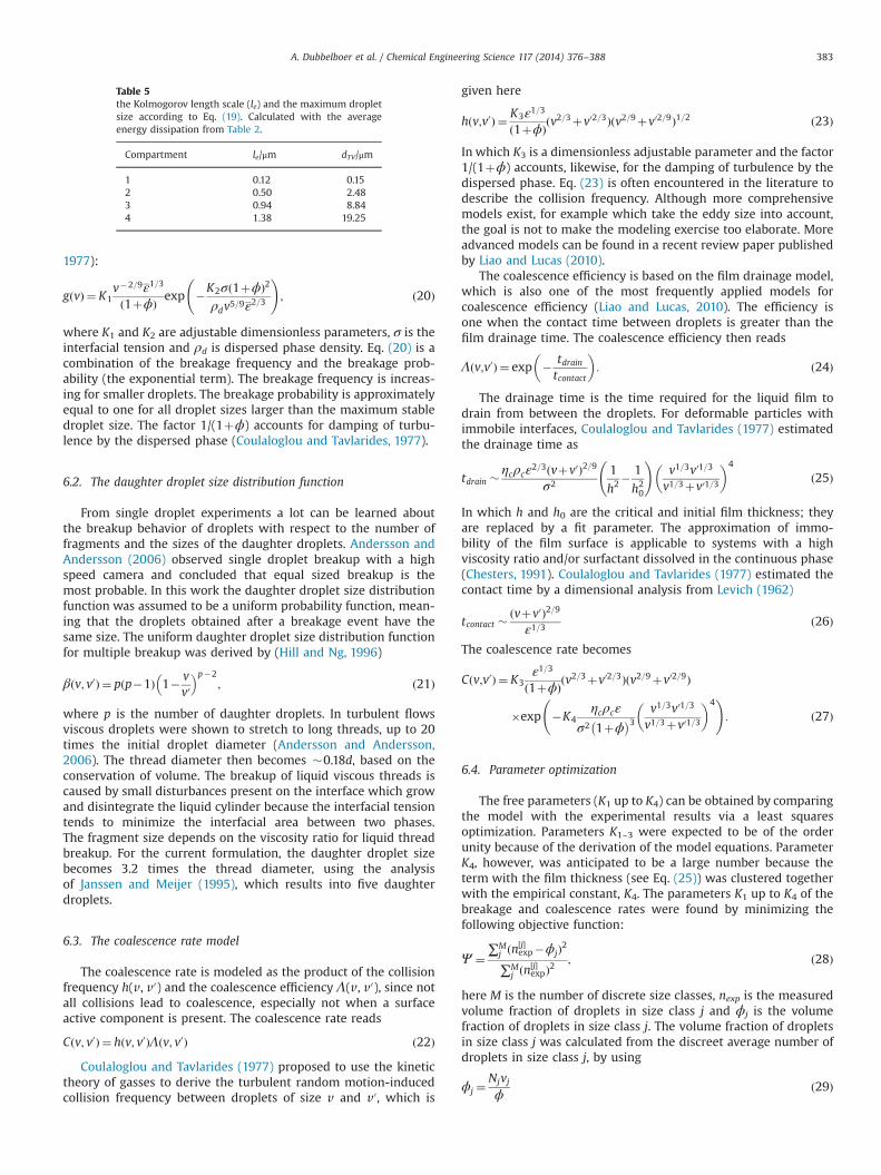
Table 5the Kolmogorov length scale (le) and the maximum dropletsize according to Eq. (19). Calculated with the averageenergy dissipation from Table 2.

Compartment le/μm dTV/μm

1 0.12 0.152 0.50 2.483 0.94 8.844 1.38 19.25

A. Dubbelboer et al. / Chemical Engineering Science 117 (2014) 376–388 383

The optimization problem appeared to be non-convex, for thatreason the Genetic Algorithm (Matlab (MATLAB and GlobalOptimization Toolbox R (2013)), a global non-linear optimizationalgorithm, was used to find the adjustable parameter values corre-sponding to the lowest objective function value. Two datasetswere used for the optimization of the parameters. The datasetswere the size distributions obtained from the experiments at 200and 800 bar after one pass through the homogenizer. The remain-ing datasets were used to test the performance of the model withthe fitted parameters. In all cases the objective function in Eq. (28)was used to judge the quality of the model predictions versus theexperimental observations.

7. Results and discussion

7.1. Prediction of droplet size distributions for single pass processing

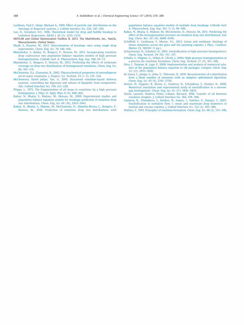
The main objective of this work was to predict the droplet sizedistributions subject to various hydrodynamic conditions in a highpressure homogenizer. This means that one set of parametersshould be able to describe the change in the droplet size distribu-tion for a range of operating conditions. The predictions of thecompartment model were compared to the measured droplet sizedistributions in Fig. 7 for four different pressures and one passthrough the homogenizer valve. Considerable improvements wereobserved when comparing the model predictions of the first passwith the results of the work of Raikar et al. (2009, 2010, 2011) orBecker et al. (2013). Note that Maindarkar et al. (2012) obtainedreasonable objective function values for the different pressures,but the fit parameters were recalculated for each pressure dropand two extra fit parameters were used.

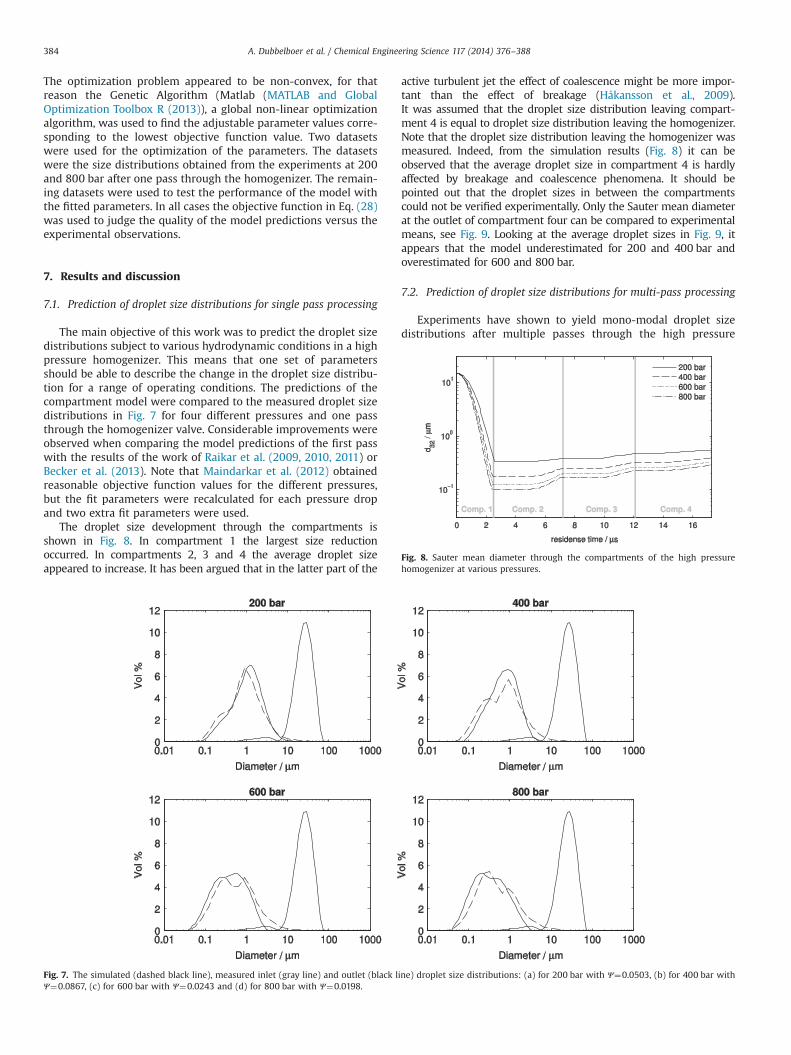
The droplet size development through the compartments isshown in Fig. 8. In compartment 1 the largest size reductionoccurred. In compartments 2, 3 and 4 the average droplet sizeappeared to increase. It has been argued that in the latter part of the

active turbulent jet the effect of coalescence might be more impor-tant than the effect of breakage (Håkansson et al., 2009).It was assumed that the droplet size distribution leaving compart-ment 4 is equal to droplet size distribution leaving the homogenizer.Note that the droplet size distribution leaving the homogenizer wasmeasured. Indeed, from the simulation results (Fig. 8) it can beobserved that the average droplet size in compartment 4 is hardlyaffected by breakage and coalescence phenomena. It should bepointed out that the droplet sizes in between the compartmentscould not be verified experimentally. Only the Sauter mean diameterat the outlet of compartment four can be compared to experimentalmeans, see Fig. 9. Looking at the average droplet sizes in Fig. 9, itappears that the model underestimated for 200 and 400 bar andoverestimated for 600 and 800 bar.

7.2. Prediction of droplet size distributions for multi-pass processing

Experiments have shown to yield mono-modal droplet sizedistributions after multiple passes through the high pressure

Fig. 7. The simulated (dashed black line), measured inlet (gray line) and outlet (black line) droplet size distributions: (a) for 200 bar with Ψ¼0.0503, (b) for 400 bar withΨ¼0.0867, (c) for 600 bar with Ψ¼0.0243 and (d) for 800 bar with Ψ¼0.0198.

Fig. 8. Sauter mean diameter through the compartments of the high pressurehomogenizer at various pressures.

A. Dubbelboer et al. / Chemical Engineering Science 117 (2014) 376–388384

homogenizer. In Fig. 10, the droplet size distributions after one,two and three passes for the four different pressures are displayed.In this simulation still the same set of parameters was used asfor the single pass experiments in Figs. 7–9. The width of thedistribution became narrower when the emulsion was passedseveral times through the homogenizer (Fig. 10). This was alsoexperimentally observed for different types of homogenizers byBecker et al. (2013) and Maindarkar et al. (2013). The populationbalance model rendered mono-modal droplet size distributionsafter two passes, but no significant change was observed after thethird pass.

The model performance was quantified by the objective func-tion value given in Eq. (28). The performances of three modelsare given in Table 7. The four compartment model was comparedto a model comprising one compartment and a model with two

compartments. In the second column the objective functionwas summed over the different operating pressures for a singlepass through the homogenizer. Increasing the number of compart-ments improved the model predictions. The model with twocompartments improved the objective function value by 33%for one pass through the homogenizer. Only considering multiplepasses the two-compartment model performed worse than theone-compartment model. Regarding all experiments, the four-compartment model performed 23% better than the one-compart-ment model.

7.3. Discussion on the fit parameters

The breakage and coalescence functions derived by Coulaloglouand Tavlarides (1977), i.e. Eqs. (20) and (27), are often used tomodel size distributions of bubbles or droplets for various types ofequipment.

The breakage and coalescence equations contain free para-meters so that the model is adjustable to many experimentalobservations. It is interesting to compare the parameters foundby other authors who used the same model for breakage andcoalescence, see Table 6. There are a lot of notable differencesbetween the different types of mixers and even for the sametype of mixer (high pressure homogenizer) the parameter valuesvary several orders of magnitude. It is, however, not possible toquantitatively compare the parameter values, because the endresult also depends on the choice of binary or multiple breakup,number of fragments and daughter droplet size distributionfunction and to a minor extent on the discretization algorithmand number of size classes. Therefore only the breakage rates as afunction of the mother droplet size are compared in Fig. 11.

The model from Raikar et al. (2010), for example, also includeda droplet breakage rate for the turbulent viscous regime andexcluded the coalescence rate. In the breakage rate for turbulentinertial breakup the damping of turbulent energy dissipation inthe breakup frequency was neglected, nonetheless parameter K1 is

Fig. 9. The measured Sauter mean diameters for four different pressures after asingle pass (bar plot) including an error bar versus the simulated droplet sizes fromthe four compartment model (triangles).

Fig. 10. The measured (continuous lines) and simulated (dashed lines) droplet size distributions for 3 passes through the homogenizer; the size distribution curves move tothe left after each pass i.e. the droplets become smaller. The simulated size distributions for passes 2 and 3 overlap.

A. Dubbelboer et al. / Chemical Engineering Science 117 (2014) 376–388 385

extremely small in comparison with all others. As a consequencethe total breakage rate is extremely small under set conditions andcannot be shown in Fig. 11. Vankova et al. (2007) used a slightlyadjusted model for their narrow gap homogenizer. Likewise, thedamping terms and coalescence rate are neglected but a factorincluding the square root of the density ratio was added. The staticmixer of Azizi and Al Taweel (2011) was divided up into severalcompartments as well and they were able to find one set ofparameters describing the full range of their experimental condi-tions. The parameter values from the original paper of Coulaloglouand Tavlarides (1977) also did not match any other set of para-meters. The reason that the parameter values deviated was thatthe energy dissipation rate near the impeller was estimated70 times the average energy dissipation.

Droplets will experience only the hydrodynamic forces in theirproximity and not the average inside a vessel or valve. In theexperiments of Maaß and Kraume (2012) single droplet breakupevents were monitored and the breakage function (Eq. (20)) wasfitted to their data. This approach offers most likely more generalparameter values. Because the breakage rate function was fitted tosingle droplet breakup events, instead of fitting the PBE to thedroplet size distribution obtained after a myriad of breakupevents. For that reason the parameters of Maaß and Kraume(2012) were tested in the population balance approach with thefour compartments. The coalescence parameters K3 and K4 were

retained from the earlier fit. The average droplet sizes were match-ing relatively well with objective function values of ΣΨ¼0.78 forthe first pass experiments and ΣΨ¼3.8 for all experiments. Butcloser inspection of the size distribution showed bimodality and awider spread of the droplet sizes.

8. Conclusions

The approach presented in this paper offered good predictionsof the complete droplet size distribution under various hydro-dynamic conditions without excessive computational times. A CFDsimulation was executed first and four compartments weredefined directly after the narrow restriction. The average energydissipation was calculated for each compartment. The energydissipation rates were included in the PBE model. The freeparameters in the model were adjusted to obtain a good fit ofthe experimental data. The extensibility of the model was tested atvarious pressures for one pass and multiple passes through thehigh pressure homogenizer at constant pressure. All in all theparameter values obtained in this work predicted the size dis-tribution well within the experimental range of the homogenizingapparatus but are expected to remain equipment dependent.

In order to have predictive control over the droplet size distri-bution in a homogenizing apparatus the hydrodynamic features areof importance. In most types of equipment there is no homo-geneous energy dissipation. There are regions where the energyintensity is high, for example close to a stirrer or inside a jet.Then it is recommended to divide up the device in so-calledcompartments in order to minimize the inhomogeneity. It has beendemonstrated here that the use of four compartments with eachhaving its own average turbulent energy dissipation improved themodel predictions by 65% compared to the single compartmentmodel. Increasing the number of compartments will evidently lead tobetter results but a penalty must be paid because the optimiza-tion time increases. The compartment approach may provide analternative to the direct coupling of population balances withComputational Fluid Dynamics. The compartment approach iscomputationally less expensive than direct coupling; moreover,direct coupling is physically questionable for geometries wherethe droplet size is equal or bigger than the confined geometry.

Nomenclature

Abbreviations

CFD Computational Fluid DynamicsPBE population balance equationsPIV Particle Image VelocimetryQMOM Quadrature Method of MomentsRANS Reynolds Averaged Navier StokesRNG Re-Normalization Group

Table 7The summed objective function (Ψ).

Model Single pass experiments All experiments

1 Compartment 0.60 4.82 Compartments 0.40 5.14 Compartments 0.21 3.7

10−8 10−7 10−6 10−5 10−4 10−30

1

2

3

4

5x 107

brea

kage

rate

/ s−1

This workVankova et al. 2007Coulaloglou & Tavlarides 1977Azizi and Al Taweel 2011Maass and Kraume 2012

diameter / m

Fig. 11. The breakage rates as a function of the droplet size from several authors; allbreakage rate functions are based on the original Eq. (20).

Table 6The obtained values for the fit parameters of the four compartment model in comparison with the work of other authors.

High pressure homogenizers Stirred vessel Static mixer Single dropletexperiment

This work: Fourcompartment model

This work: Singlecompartment model

Raikar et al.(2011)

Vankova et al.(2007)

Coulaloglou andTavlarides (1977)

Azizi and AlTaweel. (2011)

Maaß and Kraume(2012)

K1 1.47 1.81 2.62�10�8 0.033 0.40 0.86 0.91K2 1.14 0.53 0.175 3.6 0.08 4.1 0.39K3 0.087 1.99 – – 2.8 0.04 –

K4/m�2 20,420 101 – – 1.83�105 1�1010 –

A. Dubbelboer et al. / Chemical Engineering Science 117 (2014) 376–388386

Latin letters

C(v, v0) coalescence rate/m3 s�1

d droplet diameter/md32 Sauter mean diameter/mdv99 cumulative diameter, P(drdv99)¼0.99/mg(v) breakage rate/s�1

h(v, v0) collision frequency/m3 s�1

k turbulent kinetic energy/J kg�1

K1–4 fit parametersle Kolmogorov length scale/mM number of discreet size classesmc critical micelle concentration/mol m�3

nv(v,t) droplet volume fraction of size v at time tN number of size classesp number of daughter dropletsr radial coordinate/mr0 point where jet becomes self-similar/mS strain rate/s�1

t time/su fluid velocity/m s�1

u' fluid velocity fluctuation/m s�1

ū0 jet center line velocity/m s�1

U0 jet speed where the jet becomes self-similar/m s�1

v daughter droplet volume/m3

v' mother droplet volume/m3

V compartment volume/m3

xi spatial coordinates/mz axial coordinate/m

Greek letters

α entrainment coefficientβ(v, v0) daughter droplet size distribution functionΓ surface coverage/mol m�2

δ0 jet height where the jet becomes self-similar/mδij Kronecker deltaε turbulent energy dissipation rate/W kg�1

η dynamic viscosity/Pa sν kinematic viscosity/m2 sνt eddy viscosity/m2 sρ density/kg m�3

τij stresses/PaτijR Reynolds stresses/Paϕ dispersed phase volume fractionσ interfacial tension/N m�1

Ψ objective function value

Subscripts

c continuous phased dispersed phasedef deformationj index for a size classres residenceTV turbulent viscousv volume based

Acknowledgment

The authors wish to thank Unilever Research and Developmentin Vlaardingen, The Netherlands for financial support.

References

ANSYSs Fluent, 14.0, Help system, 2011. Ch. 4.13: Near-Wall Treatments for Wall-Bounded Turbulent flows, ANSYS, Inc.

Agterof, W., Vaessen, G., Haagh, G., Klahn, J., Janssen, J., 2003. Prediction ofemulsion particle sizes using a computational fluid dynamics approach.Colloids Surf. B: Biointerfaces 31 (1–4), 141–148.

Alexopoulos, A., Maggioris, D., Kiparissides., C., 2002. CFD analysis of turbulencenon-homogeneity in mixing vessels a two-compartment model. Chem. Eng. Sci.57 (10), 1735–1752.

Almeida-Rivera, C., Bongers, P., 2010. Modelling and experimental validation ofemulsification processes in continuous rotor–stator units. Comput. Chem. Eng.34 (5), 592–597.

Alopaeus, V., Koskinen, J., Keskinen, K., 1999. Simulation of the population balancesfor liquid–liquid systems in a nonideal stirred tank. Part 1 description andqualitative validation of the model. Chem. Eng. Sci. 54 (24), 5887–5899.

Andersson, R., Andersson, B., 2006. On the breakup of fluid particles in turbulentflows. AIChE J. 52 (6), 2020–2030.

Azizi, F., Al Taweel, A.M., 2011. Turbulently flowing liquid–liquid dispersions. Part I:Drop breakage and coalescence. Chem. Eng. J. 166, 715–725.

Becker, P., Dubbelboer, A., Sheibat-Othman, N., 2013. A coupled population balancecfd framework in openfoam for a high pressure homogenizer. Récents Prog.Génie Procédés 104, 2981–2988.

Blonski, S., Korczyk, P., Kowalewski, T., 2007. Analysis of turbulence in a micro-channel emulsifier. Int. J. Ther. Sci. 46 (11), 1126–1141.

Casoli, P., Vacca, A., Berta, G., 2010. A numerical procedure for predicting theperformance of high pressure homogenizing valves. Simul. Model. Pract. Theory18 (2), 125–138.

Chen, H.C., Patel, V.C., 1988. Near-wall turbulence models for complex flowsincluding separation. AIAA J. 26 (6), 641–648.

Chesters, A.K., 1991. The modelling of coalescence processes in fluid-liquid disper-sions: a review of current understanding. Trans. IChemE 69 (Part A), 259–270.

Coulaloglou, C., Tavlarides, L., 1977. Description of interaction processes in agitatedliquid–liquid dispersions. Chem. Eng. Sci. 32 (11), 1289–1297.

Davidson, P.A., 2006. Turbulence: An Introduction for Scientists and Engineers,third ed. Oxford University Press, Great Claredon Street, Oxford (Chapter 4).

Drumm, C., Attarakih, M., Bart, H.J., 2009. Coupling of cfd with dpbm for an rdcextractor. Chem. Eng. Sci. 64 (4), 721–732.

Dubbelboer, A., Janssen, J., Hoogland, H., Mudaliar, A., Zondervan, E., Bongers, P.,Meuldijk., J., 2013. A modeling approach for dispersive mixing of oil in wateremulsions. Comput. Aided Chem. Eng. 32, 841–846.

Durbin, P.A., Pettersson-Reif, B.A., 2001. Statistical Theory and Modeling forTurbulent Flows (Chapter 6). First ed. John Wiley And Sons Ltd..

Fathi Roudsari, S., Turcotte, G., Dhib, R., Ein-Mozaffari., F., 2012. Cfd modeling of themixing of water in oil emulsions. Comput. Chem. Eng. 45, 124–136.

Floury, J., Bellettre, J., Legrand, J., Desrumaux, A., 2004a. Analysis of a new type ofhigh pressure homogeniser. A study of the flow pattern. Chem. Eng. Sci. 59 (4),843–853.

Floury, J., Legrand, J., Desrumaux, A., 2004b. Analysis of a new type of high pressurehomogeniser. Part b. Study of droplet break-up and recoalescence phenomena.Chem. Eng. Sci. 59 (6), 1285–1294.

Håkansson, A., Trägårdh, C., Bergenståhl, B., 2009. Studying the effects of adsorp-tion, recoalescence and fragmentation in a high pressure homogenizer using adynamic simulation model. Food Hydrocoll. 23 (4), 1177–1183.

Håkansson, A., Fuchs, L., Innings, F., Revstedt, J., Trägårdh, C., Bergenståhl, B., 2011.High resolution experimental measurement of turbulent flow field in a highpressure homogenizer model and its implications on turbulent drop fragmen-tation. Chem. Eng. Sci. 66 (8), 1790–1801.

Håkansson, A., Fuchs, L., Innings, F., Revstedt, J., Trägårdh, C., Bergenståhl, B., 2012.Experimental validation of k–ε rans-cfd on a highpressure homogenizer valve.Chem. Eng. Sci. 71, 264–273.

Håkansson, A., Innings, F., Trägårdh, C., Bergenståhl, B., 2013a. A high pressurehomogenization emulsification model-improved emulsifier transport andhydrodynamic coupling. Chem. Eng. Sci. 91, 44–53.

Håkansson, A., Fuchs, L., Innings, F., Revstedt, J., Trägårdh, C., Bergenståhl, B., 2013b.Velocity measurements of turbulent two-phase flow in a high-pressure homo-genizer model. Chem. Eng. Commun. 200 (1), 93–114.

Hill, P., Ng, K., 1996. Statistics of multiple particle breakage. AIChE J. 42 (6), 1600–1611.Innings, F., Trägårdh, C., 2007. Analysis of the flow field in a high pressure

homogenizer. Exp. Ther. Fluid Sci. 32 (2), 345–354.Janssen, J.M.H., Meijer, H.E.H., 1995. Dynamics of liquid–liquid mixing: a 2-zone

model. Polym. Eng. Sci. 35 (22), 1766–1780.John, V., Angelov, I., Öncül, A., Thévenin, D., 2007. Techniques for the reconstruction

of a distribution from a finite number of its moments. Chem. Eng. Sci. 62 (11),2890–2904.

Karbstein, H., Schubert, H., 1995. Developments in the continuous mechanicalproduction of oil-in-water macro-emulsions. Chem. Eng. Process.: ProcessIntensif. 34 (3), 205–211.

Kumar, S., Ramkrishna, D., 1996. On the solution of population balance equations bydiscretization – I. A fixed pivot technique. Chem. Eng. Sci. 51 (8), 1311–1332.

Levich, V.G., 1962. Physicochemical Hydrodynamics. Prentice-Hall, Englewood Cliffs.Liao, Y., Lucas, D., 2009. A Literature review of theoretical models for drop and

bubble breakup in turbulent dispersions. Chem. Eng. Sci. 64 (15), 3389–3406.Liao, Y., Lucas, D., 2010. A Literature review on mechanisms and models for the

coalescence process of fluid particles. Chem. Eng. Sci. 65 (10), 2851–2864.

A. Dubbelboer et al. / Chemical Engineering Science 117 (2014) 376–388 387

Luckham, Paul F., Ukeje, Michael A., 1999. Effect of particle size distribution on therheology of dispersed systems. J. Colloid Interface Sci. 220, 347–356.

Luo, H., Svendsen, H.F., 1996. Theoretical model for drop and bubble breakup inturbulent dispersions. AIChE J. 42 (5), 1225–1233.

MATLAB and Global Optimization Toolbox R, 2013. The MathWorks, Inc., Natick,Massachusetts, United States.

Maaß, S., Kraume, M., 2012. Determination of breakage rates using single dropexperiments. Chem. Eng. Sci. 70, 146–164.

Maindarkar, S., Raikar, N., Bongers, P., Henson, M., 2012. Incorporating emulsiondrop coalescence into population balance equation models of high pressurehomogenization. Colloids Surf. A: Physicochem. Eng. Asp. 396, 63–73.

Maindarkar, S., Bongers, P., Henson, M., 2013. Predicting the effects of surfactantcoverage on drop size distributions of homogenized emulsions. Chem. Eng. Sci.89, 102–114.

McClements, D.J., Chanamai, R., 2002. Physicochemical properties of monodisperseoil-in-water emulsions. J. Dispers. Sci. Technol. 23 (1–3), 125–134.

McClements, David Julian, Yan, Li, 2010. Structured emulsion-based deliverysystems: controlling the digestion and release of lipophilic food components.Adv. Colloid Interface Sci. 159, 213–228.

Phipps, L., 1975. The fragmentation of oil drops in emulsions by a high pressurehomogenizer. J. Phys. D: Appl. Phys. 8 (4), 448–462.

Raikar, N., Bhatia, S., Malone, M., Henson, M., 2009. Experimental studies andpopulation balance equation models for breakage prediction of emulsion dropsize distributions. Chem. Eng. Sci. 64 (10), 2433–2447.

Raikar, N., Bhatia, S., Malone, M., McClements, D., Almeida-Rivera, C., Bongers, P.,Henson, M., 2010. Prediction of emulsion drop size distributions with

population balance equation models of multiple drop breakage. Colloids Surf.A: Physicochem. Eng. Asp. 361 (1–3), 96–108.

Raikar, N., Bhatia, S., Malone, M., McClements, D., Henson, M., 2011. Predicting theeffect of the homogenization pressure on emulsion drop size distributions. Ind.Eng. Chem. Res. 50 (10), 6089–6100.

Scheffold, F., Cardinaux, F., Mason, T.G., 2013. Linear and nonlinear rheology ofdense emulsions across the glass and the jamming regimes. J. Phys.: Condens.Matter 25, 502101 (5 pp.).

Schuchmann, H., Schubert, H., 2001. Emulsification in high-pressure homogenizers.Chem. Eng. Technol. 24 (10), 151–157.

Schultz, S., Wagner, G., Urban, K., Ulrich, J., 2004. High-pressure homogenization asa process for emulsion formation. Chem. Eng. Technol. 27 (4), 361–368.

Silva, L., Damian, R., Lage, P., 2008. Implementation and analysis of numerical solu-tion of the population balance equation in cfd packages. Comput. Chem. Eng.32 (12), 2933–2945.

de Souza, L., Janiga, G., John, V., Thévenin, D., 2010. Reconstruction of a distributionfrom a finite number of moments with an adaptive splinebased algorithm.Chem. Eng. Sci. 65 (9), 2741–2750.

Steiner, H., Teppner, R., Brenn, G., Vankova, N., Tcholakova, S., Denkov, N., 2006.Numerical simulation and experimental study of emulsification in a narrow-gap homogenizer. Chem. Eng. Sci. 61 (17), 5841–5855.

Taisne, Laurent, Walstra, Pieter, Cabane, Bernard, 1996. Transfer of oil betweenemulsion droplets. J. Colloid Interface Sci. 184, 378–390.

Vankova, N., Tcholakova, S., Denkov, N., Ivanov, I., Vulchev, V., Danner, T., 2007.Emulsification in turbulent flow. 1. mean and maximum drop diameters ininertial and viscous regimes. J. Colloid Interface Sci. 312 (2), 363–380.

Walstra, P., 1993. Principles of emulsion formation. Chem. Eng. Sci. 48 (2), 333–349.

A. Dubbelboer et al. / Chemical Engineering Science 117 (2014) 376–388388