Populating dark matter haloes with galaxies: comparing the ...€¦ · (PVD) that are ∼400 km...

Mon. Not. R. Astron. Soc. 350, 1153–1173 (2004) doi:10.1111/j.1365-2966.2004.07744.x

Populating dark matter haloes with galaxies: comparing the 2dFGRSwith mock galaxy redshift surveys

Xiaohu Yang,1,2� H. J. Mo,2,3� Y. P. Jing,4 Frank C. van den Bosch3

and YaoQuan Chu1

1Centre for Astrophysics, University of Science and Technology of China, Hefei, Anhui 230026, China2Department of Astronomy, University of Massachusetts, Amherst MA 01003-9305, USA3Max-Planck-Institut fur Astrophysik Karl-Schwarzschild-Strasse 1, 85748 Garching, Germany4Shanghai Astronomical Observatory; the Partner Group of MPA, Nandan Road 80, Shanghai 200030, China

Accepted 2004 February 18. Received 2004 February 9; in original form 2003 December 15

ABSTRACTIn two recent papers, we developed a powerful technique to link the distribution of galaxiesto that of dark matter haloes by considering halo occupation numbers as a function of galaxyluminosity and type. In this paper we use these distribution functions to populate dark matterhaloes in high-resolution N-body simulations of the standard �CDM cosmology with �m =0.3, �� = 0.7 and σ 8 = 0.9. Stacking simulation boxes of 100 h−1 Mpc and 300 h−1 Mpcwith 5123 particles each we construct mock galaxy redshift surveys out to a redshift of z = 0.2with a numerical resolution that guarantees completeness down to 0.01L∗. We use these mocksurveys to investigate various clustering statistics. The predicted two-dimensional correlationfunction ξ (rp, π ) reveals clear signatures of redshift space distortions. The projected correlationfunctions for galaxies with different luminosities and types, derived from ξ (rp, π ), match theobservations well on scales larger than ∼3 h−1 Mpc. On smaller scales, however, the modeloverpredicts the clustering power by about a factor two. Modelling the ‘finger-of-God’ effecton small scales reveals that the standard �CDM model predicts pairwise velocity dispersions(PVD) that are ∼400 km s−1 too high at projected pair separations of ∼1 h−1 Mpc. A strongvelocity bias in massive haloes, with bvel ≡ σ gal/σ dm ∼ 0.6 (where σ gal and σ dm are the velocitydispersions of galaxies and dark matter particles, respectively) can reduce the predicted PVDto the observed level, but does not help to resolve the overprediction of clustering power onsmall scales. Consistent results can be obtained within the standard �CDM model only whenthe average mass-to-light ratio of clusters is of the order of 1000 (M/L)� in the B-band.Alternatively, as we show by a simple approximation, a �CDM model with σ 8 � 0.75 mayalso reproduce the observational results. We discuss our results in light of the recent WMAPresults and the constraints on σ 8 obtained independently from other observations.

Key words: methods: statistical – galaxies: haloes – dark matter – large-scale structure ofUniverse.

1 I N T RO D U C T I O N

The distribution of galaxies contains important information aboutthe large-scale structure of the matter distribution. On large, linearscales the galaxy power spectrum is believed to be proportional tothe matter power spectrum, therewith providing useful informationregarding the initial conditions of structure formation, i.e. regardingthe power spectrum of primordial density fluctuations. On smaller,non-linear scales the distribution and motion of galaxies is governed

�E-mail: [email protected] (XY); [email protected] (HJM)

by the local gravitational potential, which is cosmology-dependent.One of the main goals of large galaxy redshift surveys is thereforeto map the distribution of galaxies as accurately as possible, over aslarge a volume as possible. The Sloan Digital Sky Survey (SDSS;York et al. 2000) and the 2 degree Field Galaxy Redshift Survey(2dFGRS; Colless et al. 2001) are two of the prime examples. Thesesurveys, which are currently being completed, will greatly enhanceand improve our knowledge of large-scale structure and will becomethe standard data sets against which to test our cosmological andgalaxy-formation models for the decade to come.

However, two effects complicate a straightforward interpretationof the data. First of all, the distribution of galaxies is likely to be

C© 2004 RAS

1154 X. Yang et al.

biased with respect to the underlying mass density distribution. Thisbias is an imprint of various complicated physical processes relatedto galaxy formation such as gas cooling, star formation, merging,tidal stripping and heating, and a variety of feedback processes. Infact, it is expected that the bias depends on scale, redshift, galaxytype, galaxy luminosity, etc. (Kauffmann, Nusser & Steinmetz 1997;Jing, Mo & Borner 1998; Somerville et al. 2001; van den Bosch,Yang & Mo 2003a). Therefore, in order to translate the observedclustering of galaxies into a measure for the clustering of (dark)matter, one needs to either understand galaxy formation in detail,or use an alternative method to describe the relationship betweengalaxies and dark matter (haloes). One of the main goals of this paperis to advocate one such method and to show its potential strengthfor advancing our understanding of large-scale structure.

Secondly, because of the peculiar velocities of galaxies, the clus-tering of galaxies observed in redshift space is distorted with re-spect to the real-space clustering (e.g. Davis & Peebles 1983; Kaiser1987; Regos & Geller 1991; Hamilton 1992; van de Weygaert & vanKampen 1993). On small scales, the virialized motion of galaxieswithin dark matter haloes smears out structure along the line-of-sight (i.e. the so-called ‘finger-of-God’ effect). On large scales, co-herent flows induced by the gravitational action of large-scale struc-ture enhance structure along the line-of-sight. Both effects cause ananisotropy in the two-dimensional, two-point correlation functionξ (rp, π ), with rp and π the pair separations perpendicular and paral-lel to the line-of-sight, respectively. The large-scale flows compressthe contours of ξ (rp, π ) in the π -direction by an amount that dependson β ≡ �0.6

m /b. The small-scale peculiar motions imply that ξ (rp,π ) is convolved in the π -direction by the distribution of pairwisevelocities, f (v12). Thus, the detailed structure of ξ (rp, π ) containsinformation regarding the universal matter density �m, the (linear)bias of galaxies b, and the pairwise velocity distribution f (v12).

From the above discussion it is obvious that understanding galaxybias is an integral part of understanding large-scale structure. Oneway to address galaxy bias without a detailed theory of how galax-ies form is to model halo occupation statistics. One simply specifieshalo occupation numbers, 〈N(M)〉, which describe how many galax-ies on average occupy a halo of mass M. Many recent investigationshave used such halo occupation models to study various aspectsof galaxy clustering (Jing, Mo & Borner 1998; Peacock & Smith2000; Seljak 2000; Scoccimarro et al. 2001; White 2001; Berlind& Weinberg 2002; Bullock, Wechsler, & Somerville 2002; Jing,Borner & Suto 2002; Kang et al. 2002; Marinoni & Hudson 2002;Scranton 2002; Zheng et al. 2002; Kochanek et al. 2003). In tworecent papers, Yang, Mo & van den Bosch (2003, hereafter Paper I)and van den Bosch et al. (2003a, hereafter Paper II) have taken thishalo occupation approach one step further by considering the occu-pation as a function of galaxy luminosity and type. They introducedthe conditional luminosity function (hereafter CLF) (L | M) dL ,which gives the number of galaxies with luminosities in the rangeL ± dL/2 that reside in haloes of mass M. The advantage of thisCLF over the halo occupation function 〈N(M)〉 is that it allows oneto address the clustering properties of galaxies {as a function ofluminosity}. In addition, the CLF yields a direct link between thehalo mass function and the galaxy luminosity function, and allowsa straightforward computation of the average luminosity of galaxiesresiding in a halo of given mass. Therefore, (L | M) is not onlyconstrained by the clustering properties of galaxies, as is the casewith 〈N(M)〉, but also by the observed luminosity functions (LFs)and the halo mass-to-light ratios.

In Papers I and II we used the observed LFs and the luminosity-and type-dependence of the galaxy two-point correlation function to

constrain the CLF in the standard �CDM cosmology. In this paper,we use this CLF to populate dark matter haloes in high-resolutionN-body simulations. The ‘virtual universes’ thus obtained are usedto construct mock galaxy redshift surveys with volumes and appar-ent magnitude limits similar to those in the 2dFGRS. This is thefirst time that realistic mock surveys have been constructed that (i)associate galaxies with dark matter haloes, (ii) are independent of amodel of how galaxies form, and (iii) automatically have the correctgalaxy abundances and correlation lengths as a function of galaxyluminosity and type. In the past, mock galaxy redshift surveys wereconstructed either by associating galaxies with dark matter particles(rather than haloes) using a completely {ad hoc} bias scheme (Coleet al. 1998), or by linking semi-analytical models for galaxy forma-tion (with all their associated uncertainties) to the merger histories ofdark matter haloes derived from numerical simulations (Kauffmannet al. 1999; Mathis et al. 2002).

We use our mock galaxy redshift survey to investigate a numberof statistical measures of the large-scale distribution of galaxies. Inparticular, we focus on the two-point correlation function in red-shift space, its distortions on small and large scales, and the galaxypairwise peculiar velocities. Where possible we compare our pre-dictions with the 2dFGRS and we discuss the sensitivity of theseclustering statistics to several details regarding the halo occupationstatistics. We show that the halo occupation obtained analyticallycan reliably be implemented in N-body simulations. We find that thestandard �CDM model, together with the halo occupation we haveobtained, can reproduce many of the observational results. However,we find a significant discrepancy between the model predictions andobservations on small scales. We show that to get consistent resultson small scales, either the mass-to-light ratios for clusters of galax-ies are significantly higher than normally assumed, or the linearpower spectrum has an amplitude that is significantly lower than its‘concordance’ value.

This paper is organized as follows. In Section 2 we review theCLF formalism developed in Papers I and II. Section 3 introducesthe N-body simulations and describes our method of populatingdark matter haloes in these simulations with galaxies of differenttype and luminosity. Section 4 investigates several clustering statis-tics in real space and focuses on the accuracy with which mockgalaxy distributions can be constructed using our CLF formalism.In Section 5 we use these mock galaxy distributions to constructmock galaxy redshift surveys that are comparable in size with the2dFGRS. We extract the redshift-space two-point correlation func-tion from this mock redshift survey, investigate its anisotropies in-duced by the galaxy peculiar motions, and compare our results tothose obtained from the 2dFGRS by Hawkings et al. (2003). InSection 6 we discuss possible ways to alleviate the discrepancy be-tween model and observations on small scales, and we summarizeour results in Section 7.

2 T H E C O N D I T I O NA LL U M I N O S I T Y F U N C T I O N

In Paper I we developed a formalism, based on the conditional lu-minosity function (L | M), to link the distribution of galaxies tothat of dark matter haloes. We introduced a parametrized form for (L | M) which we constrained using the LF and the correlationlengths as a function of luminosity. In Paper II we extended thisformalism by constructing separate CLFs for early- and late-typegalaxies. In this paper we use these results to populate dark matterhaloes, obtained from large numerical simulations, with both early-and late-type galaxies of different luminosities. For completeness,

C© 2004 RAS, MNRAS 350, 1153–1173

Populating dark matter haloes with galaxies 1155

we briefly summarize here the main ingredients of the CLF formal-ism, and refer the reader to Papers I and II for more details.

The conditional luminosity function is parametrized by aSchechter function:

(L|M) dL = ∗

L∗

(L

L∗

)α

exp(−L/L∗) dL, (1)

where L∗ = L∗(M), α = α(M) and ∗ = ∗(M) are all functionsof halo mass M.1 Following Papers I and II, we write the averagetotal mass-to-light ratio of a halo of mass M as⟨

M

L

⟩(M) = 1

2

(M

L

)0

[(M

M1

)−γ1

+(

M

M1

)γ2]

, (2)

which has four free parameters: a characteristic mass M1, for whichthe mass-to-light ratio is equal to (M/L)0, and two slopes, γ 1 andγ 2, that specify the behaviour of 〈M/L〉 at the low- and high-massends, respectively. A similar parametrization is adopted for the char-acteristic luminosity L∗(M):

M

L∗(M)= 1

2

(M

L

)0

f (α)

[(M

M1

)−γ1

+(

M

M2

)γ3]

, (3)

with

f (α) = �(α + 2)

�(α + 1, 1). (4)

Here �(x) is the gamma function and �(a, x) the incomplete gammafunction. This parametrization has two additional free parameters:a characteristic mass M2 and a power-law slope γ 3. For α(M) weadopt a simple linear function of log(M):

α(M) = α15 + η log(M15), (5)

with M15 the halo mass in units of 1015 h−1 M�, α15 = α(M15 = 1),and η describes the change of the faint-end slope α with halo mass.Note that once α(M) and L∗(M) are given, the normalization of theconditional LF, ∗(M), is obtained through equations (1) and (2),using the fact that the total (average) luminosity in a halo of massM is

〈L〉(M) =∫ ∞

0

(L|M)L dL = ∗ L∗�(α + 2). (6)

Finally, we introduce the mass-scale Mmin below which we set theCLF to zero; i.e. we assume that no stars form inside haloes withM < M min. Motivated by reionization considerations (see Paper Ifor details) we adopt M min = 109 h−1 M� throughout.

In order to split the galaxy population into early and late types,we follow Paper II and introduce the function f late(L, M), whichspecifies the fraction of galaxies with luminosity L in haloes ofmass M that are late type. The CLFs of late- and early-type galaxiesare then given by

late(L | M) dL = flate(L, M) (L | M) dL (7)

and

early(L | M) dL = [1 − flate(L, M)] (L | M) dL. (8)

As with the CLF for the entire population of galaxies, late(L | M)and early(L | M) are constrained by 2dFGRS measurements of theLFs and the correlation lengths as a function of luminosity. Weassume that f late(L, M) has a quasi-separable form

flate(L, M) = g(L)h(M)q(L, M). (9)

1 Halo masses are defined as the masses within the radius r180 inside ofwhich the average overdensity is 180.

Here

q(L, M) =

1 if g(L)h(M) � 11

g(L)h(M)if g(L)h(M) > 1

(10)

is to ensure that f late(L , M) � 1. We adopt

g(L) = late(L)

(L)

∫ ∞0

(L | M)n(M) dM∫ ∞0

(L | M)h(M)n(M) dM(11)

where n(M) is the halo mass function (Sheth & Tormen 1999; Sheth,Mo & Tormen 2001), late(L) and (L) correspond to the observedLFs of the late-type and entire galaxy samples, respectively, and

h(M) = max

{0, min

[1,

(log(M/Ma)

log(Mb/Ma)

)]}(12)

with Ma and Mb two additional free parameters, defined as themasses at which h(M) takes on the values 0 and 1, respectively.As shown in Paper II, this parametrization allows the population ofgalaxies to be split into early and late types such that their respectiveLFs and clustering properties are well fitted.

In Papers I and II we presented a number of different CLFs fordifferent cosmologies and different assumptions regarding the freeparameters. In what follows we focus on the flat �CDM cosmologywith �m = 0.3, �� = 0.7 and h = H 0/(100 km s−1 Mpc−1) = 0.7and with initial density fluctuations described by a scale-invariantpower spectrum with normalization σ 8 = 0.9. These cosmologicalparameters are in good agreement with a wide range of observa-tions, including the recent Wilkinson Microwave Anisotropy Probe(WMAP) results (Spergel et al. 2003), and in what follows we referto it as the ‘concordance’ cosmology. Finally, we adopt the CLF withthe following parameters: M 1 = 1010.94 h−1 M�, M 2 = 1012.04 h−1

M�, Ma = 1017.26 h−1 M�, Mb = 1010.86 h−1 M�, (M/L)0 = 124 h(M/L)�, γ 1 = 2.02, γ 2 = 0.30, γ 3 = 0.72, η = −0.22 and α15 =−1.10. This model (referred to as model D in Paper II) yields ex-cellent fits to the observed LFs and the observed correlation lengthsas a function of both luminosity and type.2

3 P O P U L AT I N G H A L O E S W I T H G A L A X I E S

3.1 Numerical simulations

The main goal of this paper is to use the CLF described in the previ-ous section to construct mock galaxy redshift surveys, and to studya number of statistical properties of these distributions that can becompared with observations from existing or forthcoming redshiftsurveys. The distribution of dark matter haloes is obtained from aset of large N-body simulations (dark matter only). The set con-sists of a total of six simulations with N = 5123 particles each, that

2 Note that the parameters listed here are slightly different from those givenin the original version of Paper II, as they are based on a corrected version ofthe galaxy luminosity function. As shown in Paper I, a change in the overallamplitude of the luminosity function in the fitting has some effect on thebest-fitting values of the correlation lengths. This is due to the combinationof the following two effects. First, our model assumes a fixed mass-to-lightratio for massive haloes and so a change in the amplitude of the luminosityfunction leads to a change in the relative number of galaxies in small/largehaloes. Second, although the correlation length as a function of luminositywas used as input in our fitting of the conditional luminosity function, thereis some freedom for the ‘best-fitting’ values of the correlation lengths tochange in the fitting, because the error bars on the observed correlationlengths are quite large.

C© 2004 RAS, MNRAS 350, 1153–1173

1156 X. Yang et al.

Figure 1. The left-hand panel plots the halo mass functions of the numerical simulations discussed in the text (histograms). The mass function with a lowmass cut at about 2 × 1011 h−1 M� corresponds to a simulation with L box = 300 h−1 Mpc, while the other corresponds to a L100 simulation with L box =100 h−1 Mpc. The solid curve is the Sheth et al. (2001) mass function which is shown for comparison. Note the excellent agreement, both between the twosimulations and between the simulation results and the theoretical prediction. The right-hand panel plots the conditional probability distributions P(M | L) forfour different luminosities as indicated. L∗ = 1.1 × 1010 h−2 L� is the characteristic luminosity of the Schechter fit to the 2dFGRS LF of Madgwick et al.(2002). Combining these conditional probability distributions with the halo mass functions shown in the left-hand panel gives an indication of the completenesslevel that can be obtained with both the L100 and L300 simulations (see text).

have been carried out on the VPP5000 Fujitsu supercomputer of theNational Astronomical Observatory of Japan with the vectorized-parallel P3M code (Jing & Suto 2002). Each simulation evolves thedistribution of the dark matter from an initial redshift of z = 72down to z = 0 in a �CDM ‘concordance’ cosmology. All simu-lations consider boxes with periodic boundary conditions; in twocases L box = 100 h−1 Mpc while the other four simulations all haveL box = 300 h−1 Mpc. Different simulations with the same box sizeare completely independent realizations and are used to estimateerrors due to cosmic variance. The particle masses are 6.2 × 108

h−1 M� and 1.7 × 1010 h−1 M� for the small- and large-box sim-ulations, respectively. One of the simulations with L box = 100 h−1

Mpc has previously been used by Jing & Suto (2002) to derive atriaxial model for density profiles of CDM haloes, and we refer thereader to that paper for complementary information about the sim-ulations. In what follows we refer to simulations with L box = 100h−1 Mpc and L box = 300 h−1 Mpc as L100 and L300 simulations,respectively.

Dark matter haloes are identified using the standard friends-of-friends (FOF) algorithm (Davis et al. 1985) with a linking length of0.2 times the mean interparticle separation. Haloes obtained withthis linking length have a mean overdensity of ∼180 (Porciani,Dekel & Hoffman 2002), in good agreement with the definitionof halo masses used in our CLF analysis. For each individual simu-lation we construct a catalogue of haloes with 10 particles or more,for which we store the mass (number of particles), the position of themost bound particle, and the mean velocity of the halo and velocitydispersion. Note that the FOF algorithm can sometimes select poorsystems (those with a small number of particles) that are spuriousand have abnormally large velocity dispersions. We have thereforemade a check to make sure that the particles assigned to a systemaccording to the FOF algorithm are gravitationally bound. Our testshowed that this correction is important only for low-mass haloes,and that it has almost no effect on our results. The left panel ofFig. 1 plots the z = 0 halo mass functions for one of the L100 sim-ulations and for one of the L300 simulations (histograms), with allspurious haloes erased. For comparison, we also plot (solid line)the analytical halo mass function given in Sheth & Tormen (1999)

and Sheth et al. (2001).3 The agreement is remarkably good, bothbetween the two simulations and between the simulation results andthe theoretical prediction.

Note that our choice for box sizes of 100 h−1 Mpc and 300 h−1

Mpc is a compromise between high mass resolution and a suffi-ciently large volume to study the large-scale structure. The impact ofmass resolution is apparent from considering the conditional prob-ability function

P(M | L) dM = (L | M)

(L)n(M) dM, (13)

(see Paper I), which gives the probability that a galaxy of luminosityL resides in a halo with mass in the range M ± dM/2. The rightpanel of Fig. 1 plots this probability distribution obtained from theCLF given in Section 2 for four different luminosities: L = L∗/100,L = L∗/10, L = L∗ and L = 10L∗. Whereas 10 L∗ galaxies are typ-ically found in haloes with 1013 h−1 � M � 1015 h−1 M�, galaxieswith L = L∗/100 ∼ 108 h−2 L� typically reside in haloes of M � 5× 1010 h−1 M�. Comparing these probability distributions with thehalo mass functions in the left panel, we see that the L300 simulationscan only yield a complete galaxy distribution down to L ∼ 0.4L∗.The L100 simulation, however, resolves dark matter haloes down tomasses of 1010 h−1 M�, which is sufficient to model the galaxy pop-ulation down to L ∼ 0.01L∗. On the other hand, luminous galaxiesmay be underrepresented in this small-box simulation, because itcontains fewer massive haloes than expected. Combining these twosets of simulations, however, will enable us to study the clusteringproperties of galaxies covering a sufficiently large volume and asufficiently large range of luminosities.

3.2 Halo occupation numbers

When populating haloes with galaxies based on the CLF one firstneeds to choose a minimum luminosity. Based on the mass resolu-tion of the simulations we adopt L min = 107 h−2 L� throughout.The mean occupation number of galaxies with L � L min for a halo

3 This same mass function is used in the CLF analysis described in Section 2.

C© 2004 RAS, MNRAS 350, 1153–1173


with mass M then follows from the CLF according to:

〈N (M)〉 =∫ ∞

Lmin

(L | M) dL. (14)

In order to Monte Carlo sample occupation numbers for individualhaloes one requires the full probability distribution P(N | M) (withN an integer) of which 〈N(M)〉 gives the mean, i.e.

〈N (M)〉 =∞∑

N=0

N P(N | M). (15)

As a simple model we adopt

P(N | M) =

N ′ + 1 − 〈N (M)〉 if N = N ′

〈N (M)〉 − N ′ if N = N ′ + 1

0 otherwise.

(16)

Here N ′ is the largest integer smaller than 〈N(M)〉. Thus, the actualnumber of galaxies in a halo of mass M is either N ′ or N ′ + 1. Thisparticular model for the distribution of halo occupation numbers issupported by semi-analytical models and hydrodynamical simula-tions of structure formation (Benson et al. 2000; Berlind et al. 2003)which indicate that the halo occupation probability distribution isnarrower than a Poisson distribution with the same mean. In addi-tion, distribution (16) is successful in yielding power-law correlationfunctions, much more so than, for example, a Poisson distribution(Benson et al. 2000; Berlind & Weinberg 2002).

3.3 Assigning galaxies their luminosity and type

Since the CLF only gives the average number of galaxies with lu-minosities in the range L ± dL/2 in a halo of mass M, there aremany different ways in which one can assign luminosities to the Ni

galaxies of halo i, and yet be consistent with the CLF. The simplestapproach would be simply to draw Ni luminosities (with L > L min)randomly from (L | M). Alternatively, one could use a more de-terministic approach, and, for instance, always demand that the j thbrightest galaxy has a luminosity in the range [Lj, Lj−1]. Here Lj isdefined such that a halo has on average j galaxies with L > Lj, i.e.∫ ∞

L j

(L | M) dL = j . (17)

We adopt an intermediate approach in most of our discussion, givingspecial treatment only to the one brightest galaxy per halo. Theluminosity of this so-called ‘central’ galaxy, Lc, is drawn from (L|M) with the restriction L > L 1 and thus has an expectation value of

〈Lc(M)〉 =∫ ∞

L1

(L | M)L dL = ∗ L∗�(α + 2, L1/L∗). (18)

The remaining Ni − 1 galaxies are referred to as ‘satellite’ galaxiesand are assigned luminosities in the range L min < L < L 1, againdrawn from the distribution function (L | M). In Section 4.2,we test the effect of luminosity sampling by comparing the resultsobtained from all the three approaches.

Finally, the galaxies are assigned morphological types as follows.For each galaxy with luminosity L in a halo of mass M we draw arandom number R in the range [0, 1]. If R < flate(L, M) then thegalaxy is a late type, otherwise an early type.

3.4 Assigning galaxies their phase-space coordinates

Once the population of galaxies has been assigned luminosities andtypes, they need to be assigned a position within their halo as well

as a peculiar velocity. The central galaxy is assumed to be located atthe ‘centre’ of the corresponding dark halo, which we associate withthe position of the most-bound particle, and its peculiar velocity isset equal to the mean halo velocity (cf. Yoshikawa, Jing & Borner2003). For the satellite galaxies we follow two different approaches.In the first, we assign the Ni − 1 satellites the positions and peculiarvelocities of Ni − 1 randomly selected dark matter particles thatare part of the FOF halo under consideration. This thus correspondsto a scenario in which satellite galaxies are completely unbiasedwith respect to the density and velocity distribution of dark matterparticles in FOF haloes. We refer to satellite galaxies populated thisway as ‘FOF satellites’.

We also consider a more analytical model for the satellite distribu-tion. This allows us first of all to assess whether a simple analyticaldescription can be found to describe the population of satellite galax-ies, and secondly, provides us with a simple framework to investigatethe sensitivity of various clustering statistics to details regarding thedensity and velocity bias of satellite galaxies. We assume that thenumber density distribution of satellite galaxies follows a NFWdensity distribution (Navarro, Frenk & White 1997):

ρ(r ) = δρ

(r/rs)(1 + r/rs)2, (19)

where rs is a characteristic radius, ρ is the average density of theUniverse, and δ is a dimensionless amplitude which can be expressedin terms of the halo concentration parameter c = r 180/r s as

δ = 180

3

c3

ln(1 + c) − c/(1 + c). (20)

Here r180 is the radius inside of which the halo has an average over-density of 180. Numerical simulations show that halo concentrationdepends on halo mass, and we use the relation given by Bullocket al. (2001), converted to the c appropriate for our definition ofhalo mass. The radial number density distribution of satellite galax-ies is assumed to follow equation (19) with a concentration cg = c,and the angular position is assumed to be random over the 4π solidangle. Peculiar velocities are assumed to be the sum of the peculiar(mean) velocity of the host halo plus a random velocity which isassumed to be distributed isotropically and to follow a Gaussian,one-dimensional velocity distribution:

f (v j ) = 1√2πσgal

exp

(− v2

j

2σ 2gal

). (21)

Here vj is the velocity relative to that of the central galaxy alongthe j-axis, and σ gal is the one-dimensional velocity dispersion ofthe galaxies, which we set equal to that of the dark matter particles,σ dm, in the halo under consideration. We refer to satellite galaxiespopulated this way as ‘NFW satellites’.

4 R E S U LT S I N R E A L S PAC E

Figs 2 and 3 show slices of mock galaxy distributions (hereafterMGDs) constructed from L100 and L300 simulations, respectively.Satellite galaxies are assigned positions and velocities using theNFW scheme outlined above. Results are shown for all galaxies (up-per right panels), and separately for early types (lower-right panels)and late types (lower-left panels). For comparison, we also show thedistribution of dark matter particles in the upper-left panels. Notehow the large-scale structure in the dark matter distribution is de-lineated by the distribution of galaxies, and that early-type galaxiesare more strongly clustered than late-type galaxies.

C© 2004 RAS, MNRAS 350, 1153–1173

1158 X. Yang et al.

Early–Type Galaxies

All Galaxies

LateType–Galaxies

Dark Matter

Figure 2. Projected dark matter/galaxy distributions of a 100 × 100 × 10 h−1 Mpc slice in one of the L100 mock galaxy distributions. The panels show(clockwise from top-left) the dark matter particles, all galaxies (early plus late), early-type galaxies, and late-type galaxies. Galaxies are weighted by theirluminosities. Note how the galaxies trace the large-scale structure of the dark matter, and how early-type galaxies are more strongly clustered than late-typegalaxies.

In this section we discuss the general, real-space properties ofthese MGDs. In Section 5 below we construct mock galaxy red-shift surveys to investigate the impact of redshift distortions. Themain goal of this section, however, is to investigate with what accu-racy the combination of numerical simulations and our CLF anal-ysis can be used to construct self-consistent mock galaxy distribu-tions. In particular, we want to examine to what accuracy theseMGDs can recover the input used to constrain the CLFs. Notethat this is not a trivial question. The CLF modelling is based onthe halo model, which only yields an approximate description ofthe dark matter distribution in the non-linear regime (see the dis-cussions in Cooray & Sheth 2002; Huffenberger & Seljak 2003).In addition, as described in Section 3, the CLF alone does notyield sufficient information to construct MGDs, and we had tomake additional assumptions regarding the distribution of galaxieswithin individual haloes. A further goal of this section, therefore,is to investigate how these assumptions impact on the clusteringstatistics.

4.1 The luminosity function

The CLFs used to construct the MGDs shown in Fig. 2 and 3 areconstrained by the 2dFGRS luminosity functions for early- and late-type galaxies obtained by Madgwick et al. (2002). Therefore, as longas the halo mass function is well sampled by the simulations, theLFs of our MGDs should match those of Madgwick et al. (2002).Fig. 4 shows a comparison between the 2dFGRS LFs (symbolswith error bars) and those recovered from the MGDs (solid lines).To emphasize the level of agreement between the recovered LFs andthe input LFs, Fig. 5 plots the ratio between the two. Over a largerange of luminosities, the recovered LFs match the observationalinput extremely well. In the L300 simulation, however, the LFs areunderestimated for L � 3 × 109 h−2 L� (M bJ − 5 log h � −18.4).This is due to the absence of haloes with M � 2 × 1011 h−1 M� (seeFig. 1). Note how this discrepancy sets in at higher L for the late-typegalaxies than for the early-types, because the latter are preferentiallylocated in more massive haloes. For the early-types the L300 mock

C© 2004 RAS, MNRAS 350, 1153–1173


Figure 3. Same as Fig. 2, but for a 300 × 300 × 20 h−1 Mpc slice taken from one of the L300 mock galaxy distributions.

is virtually complete down to M bJ − 5 log h −17 (see fig. 10 ofPaper II), reflecting the fact that only a very small fraction of theearly-type galaxies brighter than this magnitude reside in haloesbelow the mass resolution limit. In the L100 simulations, on theother hand, the LFs accurately match the data down to the faintestluminosities, but here the MGD underestimates the LFs at the brightend (M bJ − 5 log h �−22). This is due to the limited box size, whichcauses the number of massive haloes (the main hosts of the brightestgalaxies) to be underestimated (cf. Fig. 1). Note that even the LFs ofthe L300 simulations underestimate the observed number of brightgalaxies. This reflects a small inaccuracy of our CLF to match theobserved bright end of the LFs accurately (see Paper II).

4.2 The real-space correlation function

In addition to the LFs of early- and late-type galaxies, the CLFs usedhere to construct our MGDs are also constrained by the luminosityand type dependence of the correlation lengths as measured from the2dFGRS by Norberg et al. (2002a). Here we check to what degreethis ‘input’ is recovered from the MGDs.

The left panel of Fig. 6 plots the real-space two-point correlationfunctions (2PCFs) for dark matter particles in the L100 (dashed line)and L300 (dotted line) simulations. The solid line corresponds tothe evolved, non-linear dark matter correlation function of Smithet al. (2003) and is shown for comparison.4 As one can see, on largescales (r � 6 h−1 Mpc) the correlation amplitude obtained fromthe L100 simulations is systematically lower than both that obtainedfrom the L300 simulations and that obtained from the fitting formulaof Smith et al., suggesting that the box-size effect is non-negligiblein the L100 simulations. Note also that the large-scale correlationamplitude given by the L300 simulations is slightly higher than themodel of Smith et al. It is unclear if this discrepancy is due tothe inaccuracy of the fitting formula, or due to cosmic variancein the present simulations. As we will see below, this discrepancylimits the accuracy of model predictions.

The right-hand panel of Fig. 6 plots the 2PCFs for the galaxiesin the L100 (dashed line) and L300 (dotted line) MGDs. Note how

4 In fitting the CLF we have used this function to compute the correlationlength of the dark matter (see Paper II).

C© 2004 RAS, MNRAS 350, 1153–1173

1160 X. Yang et al.

Figure 4. The luminosity functions of the mock galaxies constructed from the L100 (left) and L300 (right) halo catalogues (solid lines). For comparison, wealso plot the LFs obtained by Madgwick et al. (2002) for all galaxies (circles), for late-type galaxies (triangles) and for early-type galaxies (stars). For clarity,the latter two LFs have been shifted down by one and two orders of magnitude in the y-direction, respectively. Except for incompleteness effects due to thesampling of the halo mass function (see text for details), the mock galaxy distributions have LFs that are in excellent agreement with the data.

Figure 5. The ratio of the luminosity function of mock galaxies, mock(L),to that of the 2dFGRS, 2dFGRS(L) (taken from Madgwick et al. 2002). Thethin error bars indicate the errors on 2dFGRS(L). The thick solid (dashed)lines correspond to the LFs obtained from the L100 (L300) simulations. Theerror bars for the mock galaxies are obtained from the 1σ variance of thetwo L100 and the four L300 simulations, respectively. See text for discussion.

the galaxies reveal the same trend on large scales as the dark matterparticles, with larger correlations in the L300 than in the L100 MGD.

Fig. 7 shows the correlation lengths r0 as a function of luminosityfor all (upper panel), early-type (middle panel) and late-type (lowerpanel) galaxies. These have been obtained by fitting ξ (r) with apower-law relation of the form ξ (r ) = (r/r 0)−γ over the same rangeof scales as used by Norberg et al. (2002a). Solid squares and openstars correspond to correlation lengths obtained from the L300 andL100 MGDs, respectively. Note that the error bars on the predictedcorrelation lengths are based on the scatter among independent sim-ulations boxes. They are significantly smaller than the error bars onthe observational data, because the model predictions are based onreal-space correlation functions, while the observational results arebased on projected correlation functions in redshift space. The agree-ment with the data (open circles) is reasonable, even though severalsystematic trends are apparent. In particular, the correlation lengthsobtained from the L300 simulation are slightly higher than the ob-servations while the opposite applies to the L100 simulation. Thesediscrepancies are due to two effects. First of all, as shown in Fig. 6the dark matter on large scales is more strongly clustered in the L300

simulations than in the L100 simulations. That this can account formost of the differences between the scalelengths obtained from theL300 and L100 simulations, is illustrated by the dotted and solid hori-zontal lines, which indicate the correlation lengths of the dark mat-ter particles in the L300 and L100 simulations, respectively. Secondly,the measured correlation lengths correspond to a non-zero, medianredshift which is larger for the more luminous galaxies. In deter-mining the best-fitting parameters for the CLF this redshift effect istaken into account (see Papers I and II). However, in the construc-tion of our MGDs, we only use the dark matter distribution at z = 0.As discussed in Paper I, this can overestimate the correlation lengthby about 10 per cent. Given these sources of systematic errors, oneshould be careful not to overinterpret any discrepancy between thecorrelation lengths in the mock survey and those obtained from realredshift distributions.

In order to investigate the sensitivity of the 2PCF in the MGDs tothe way we assign luminosities and phase-space coordinates to the

C© 2004 RAS, MNRAS 350, 1153–1173


Figure 6. Two-point correlation functions for dark matter particles (left panel) and mock galaxies (right panel). The dotted and dashed lines correspond toresults from the L300 and L100 simulations, respectively. The solid line in the left panel corresponds to the evolved, non-linear correlation function for the darkmatter obtained by Smith et al. (2003), and is shown for comparison. Due to the limited box sizes, the L300 (L100) simulations slightly over (under) predict thecorrelation power on large scales with respect to the model of Smith et al. The 2PCFs in the right panel are calculated for galaxies with absolute magnitudesM bJ − 5 log h < −18.4, which corresponds to the completeness limit of the L300 MGDs. Note that the box size also affects the 2PCFs of the mock galaxieson large scales. Error bars are the variance among the two (L100) and four (L300) independent realizations.

galaxies within the dark matter haloes, we construct MGDs usingone of the L300 simulations with different models for the luminos-ity assignment and spatial distribution of satellite galaxies withinhaloes. We have confirmed that using one of the L100 simulations in-stead yields the same results. We first test the impact of the luminos-ity assignment. Here, instead of the fiducial model for the luminosityassignment (the intermediate approach discussed in Section 3.3), weuse both the deterministic and random assignments (see Section 3.3for definitions) to construct the MGDs. In Fig. 8 we shown the ratiosbetween the correlation functions obtained from these MGDs andthose obtained from the fiducial MGD. For bright galaxies, the de-terministic model gives the lowest amplitudes on small scales (r �1 h−1 Mpc), while the random model gives the highest amplitudes.This is expected. The mean number of bright galaxies in a typicalhalo is not much larger than 1 and so not many close pairs of brightgalaxies are expected in the deterministic model. More such pairsare expected in the random model because more than one galaxyin a typical halo can be assigned a large luminosity due to randomfluctuations. The dashed lines in Fig. 8 correspond to a MGD withFOF satellites (see Section 3.4). The agreement of the 2PCFs be-tween this MGD with FOF satellites and our fiducial MGD indicatethat the spherical NFW model is a good approximation of the aver-age density distribution of dark matter haloes. We have also testedthe impact of changing the concentration of galaxies, cg; increasing(decreasing) cg with respect to the dark matter halo concentration,c, increases (decreases) the 2PCFs on small scales (r � 1 h−1 Mpc).However, even when changing the ratio cg/c by a factor of 2, theamplitude of this change is smaller than the differences resultingfrom changing the luminosity assignment.

All in all, changes in the way we assign luminosities and phase-space coordinates to the galaxies only have a mild impact on the2PCFs, and only at small scales �1 h−1 Mpc. This is in good agree-ment with Berlind & Weinberg (2002) who have shown that theseeffects are much smaller than changes in the second moment of thehalo occupation distributions. For example, assuming a PoissonianP(N | M), rather than equation (16) has a much larger impact on

the 2PCFs than any of the changes investigated above. As we showin Section 5 below, with the P(N | M) of equation (16) we obtaincorrelation functions that are in better agreement with observations,providing empirical support for this particular occupation numberdistribution.

It is interesting to note that although small changes in the waywe assign luminosities and phase-space coordinate do not have abig impact on the statistical measurements we are considering here,such changes can lead to quite different results for other statisticalmeasures. As shown in van den Bosch et al. (in preparation), variousstatistics of satellite galaxies around bright galaxies can be used todistinguish models that make similar predictions about the clusteringon large scales.

4.3 Pairwise velocities

The peculiar velocities of galaxies are determined by the action ofthe gravitational field, and so are directly related to the matter dis-tribution in the Universe. Observationally, the properties of galaxypeculiar velocities are inferred from distortions in the correlationfunction. We defer this discussion to Section 5. Here we derive sta-tistical quantities directly from the simulated peculiar velocities ofgalaxies.

We define the pairwise peculiar velocity of a galaxy pair as

v12(r ) ≡ [v(x + r ) − v(x)] · r , (22)

with v(x) the peculiar velocity of a galaxy at x. The mean pair-wise peculiar velocity and the pairwise peculiar velocity dispersion(PVD) are

〈v12(r )〉 and σ12(r ) ≡ ⟨[v12(r ) − 〈v12(r )〉]2

⟩1/2, (23)

where 〈· · ·〉 denotes an average over all pairs of separation r.In order to gain insight, we compute 〈v12(r)〉 and σ 12(r) from the

L300 simulations for both dark matter particles and for galaxies withM bJ − 5 log h � −18.4 (which corresponds to the completenesslimit of these simulations, see Fig. 4).

C© 2004 RAS, MNRAS 350, 1153–1173

1162 X. Yang et al.

Figure 7. The real-space correlation length, r0, as a function of galaxy lumi-nosity and type. The top panel shows the results for the combined sample ofearly- plus late-type galaxies, while the middle (bottom) panel shows resultsfor the early- (late-) type galaxies only. Solid squares and stars correspondto the correlation lengths obtained from the L300 and L100 simulations, re-spectively. The error bars correspond to the 1σ variance from the two (four)independent realizations for L100 (L300). We also indicate (open circles witherror bars) the correlation lengths obtained from the 2dFGRS by Norberget al. (2002a). In the upper panel, we also plot the correlation lengths for darkmatter particles for L100 (solid line) and L300 (dotted line) simulations. Al-though the agreement between data and MGDs is reasonable there are smallbut significant differences. The reason for these discrepancies is discussedin the text.

Results are shown in Fig. 9. The upper-left panel compares themean pairwise peculiar velocities of the dark matter particles (solidcircles) with those of two realizations of the galaxies: one with‘NFW satellites’ (open circles) and the other with ‘FOF satellites’(stars). At sufficiently small separations, one probes the virializedregions of dark matter haloes, and one thus finds 〈v12〉 = 0. Atlarger separations, one starts to probe the infall regions around thevirialized haloes, yielding negative values for 〈v12(r)〉. Finally, atsufficiently large separations 〈v12(r )〉 → 0 due to the large-scalehomogeneity and isotropy of the Universe.

Both the dark matter particles and the galaxies from our MGDsindeed reveal such behaviour, with 〈v12(r)〉 peaking at ∼3 h−1 Mpc.However, there is a markedly strong difference between the 〈v12(r)〉of galaxies in the MGD with NFW satellites and that of the darkmatter. In this particular MGD, the galaxies experience significantly

Figure 8. The ratio of the 2PCF ξ (r) in three MGDs compared to that ofour fiducial MGD. The only difference among these various MGDs is theway that we assign luminosities and phase-space coordinates to the galaxies.Solid (dotted) lines correspond to a MGD in which we use a deterministic(random) method to assign galaxies their luminosities (see Section 3.3 fordefinitions). In the MGD corresponding to the dashed line we use the in-termediate, fiducial method to assign luminosities, but here we use ‘FOFsatellites’ rather than ‘NFW satellites’ (see Section 3.4 for definitions). Re-sults are shown for galaxies in three different magnitude bins (as indicated)in one of the L300 simulations. However, results for the L100 simulationslook virtually identical.

smaller infall velocities than the dark matter particles. However, thisdifference between dark matter and galaxies is almost absent in theMGD with FOF satellites. This is due to the fact that in the NFWmodel, we populate satellites with isotropic velocity dispersionswithin a sphere of radius r180. We are thus assuming that the entireregion out to r180 is virialized in that there is no net infall. However,simple collapse models predict that for our concordance cosmologyonly the region out to r340 (i.e. the radius inside of which the averageoverdensity is 340) is virialized (Bryan & Norman 1998). The dif-ference between the MGDs with NFW satellites and FOF satellitesindicates that the regions between r340 and r180 are still infalling,resulting in non-zero 〈v12〉.

In the lower-left panel, we compare the PVDs for galaxies anddark matter particles. Here the MGDs with FOF satellites and NFWsatellites are fairly similar, and significantly lower than for the darkmatter. This can be understood as follows. At small separations, thePVD is a pair-weighted measure for the potential well in which darkmatter particles (galaxies) reside. For the galaxies in our MGDs thehalo occupation number per unit mass, N/M, decreases with the

C© 2004 RAS, MNRAS 350, 1153–1173


Figure 9. The mean pairwise velocities (upper panels) and pairwise velocity dispersions (lower panels) estimated from the three-dimensional (real-space)velocities of the mock galaxies and dark matter particles. All results correspond to the L300 simulations only. Left-hand panels compare dark matter particles(solid circles) with galaxies either with NFW satellites (open circles) or with FOF satellites (open stars). Right-hand panels display the galaxy-type dependencefor a model with NFW satellites (error bars indicate the rms scatter among the four independent L300 simulations). See text for detailed discussion.

mass of dark matter haloes (see Paper II). Therefore, the massivehaloes (with larger velocity dispersions) contribute relatively less tothe PVDs of galaxies. Although the difference between the σ 12(r)of the MGDs with FOF and NFW satellites shows that the PVDshave some dependence on the details regarding the infall regionsaround virialized haloes, these effects are typically small.

The upper-right and lower-right panels of Fig. 9 show how〈v12(r)〉 and σ 12(r) depend on galaxy type. Results are shown forthe MGD based on NFW satellites. The mean velocities for early-type galaxies are larger than those for late-type galaxies on largescales, but smaller on small scales. In addition, the PVD of early-type galaxies is higher than that of late-type galaxies on all scales.All these differences are easily understood as a reflection of the factthat early-type galaxies are preferentially located in the larger, moremassive haloes which have larger velocity dispersions and largerinfall velocities.

Fig. 10 shows the pairwise velocity distributions for four differ-ent separations r, within a logarithmic interval of �log r = 0.125.On small scales, the distribution is well-fitted by an exponentialfor both dark matter particles and galaxies. This validates the as-sumption made in earlier analyses about this distribution (Davis &Peebles 1983; Mo, Jing & Borner 1993; Fisher et al. 1994; Marzkeet al. 1995). It is also consistent with earlier results obtained fromtheoretical models and numerical simulations based on dark mat-ter particles (Efstathiou et al. 1988; Diaferio & Geller 1996; Sheth1996; Mo, Jing & Borner 1997; Seto & Yokoyama 1998; Magira,Jing & Suto 2000). For larger separations f (v12) is skewed towardsnegative values of v12, because galaxies tend to approach each otherdue to gravitational infall. Clearly, a single exponential function isno longer a good approximation to the pairwise peculiar velocitydistribution at large separations. Although for v12 < 0 (infall) theexponential remains remarkably accurate, for v12 > 0 the pairwisevelocity distribution reveals a more Gaussian behaviour. This may

have important implications for the derivation of PVDs (especiallyat large separations), which typically is based on the assumption ofa purely exponential f (v12). We shall return to this issue in moredetail in Section 5.2.

5 R E S U LT S I N R E D S H I F T S PAC E

The statistical quantities of galaxy clustering discussed in the pre-vious section are based on real distances between galaxies in ourMGDs. However, because of the peculiar velocities of galaxies, suchquantities cannot be obtained directly from a galaxy redshift survey.On small scales the virialized motion of galaxies within dark matterhaloes cause a reduction of the correlation power, while on largerscales the correlations are boosted due to the infall motion of galax-ies towards overdensity regions (Kaiser 1987; Hamilton 1992). Asdiscussed in the introduction, these distortions contain useful infor-mation about the universal density parameter, the bias of galaxieson large (linear) scales, and the pairwise velocities of galaxies.

In this section, we use the MGDs presented above to constructlarge mock galaxy redshift surveys (hereafter MGRSs). The maingoals are to compare various clustering statistics from these mocksurveys with observational data from the 2dFGRS, and to investigatehow the details about the CLF and the distribution of galaxies withinhaloes impact on these statistics. For the model–data comparison weuse the large-scale structure analysis of Hawkins et al. (2003, here-after H03), which is based on a subsample of the 2dFGRS consistingof all galaxies located in the North Galactic Pole (NGP) and SouthGalactic Pole (SGP) survey strips with redshift 0.01 � z � 0.20 andapparent magnitude bJ < 19.3. This sample consists of ∼166 000galaxies covering an area on the sky of ∼1090 deg2.

In order to carry out a proper comparison between model and ob-servation, we aim to construct MGRSs that have the same selectionsas the 2dFGRS. First of all, the survey depth of zmax = 0.2 implies

C© 2004 RAS, MNRAS 350, 1153–1173

1164 X. Yang et al.

Figure 10. Distribution of pairwise velocities, f (v12), for dark matter particles (solid curves), and for mock galaxies in the L300 simulation. Results are shownfor four separations r as indicated, and for all galaxies (dot-dashed lines), early-type galaxies (dotted lines) and late-type galaxies (dashed lines). On smallscales (r < 1 h−1 Mpc) the pairwise velocity distributions are symmetric and reveal an obvious exponential form. On larger scales, however, f (v12) revealsclear asymmetries: for v12 < 0 the distribution is still close to an exponential, while for v12 > 0 the distribution more resembles a normal distribution.

that we need to cover a volume with a depth of 600 h−1 Mpc, i.e.twice that of our big L300 simulations. In principle, we could stack4 × 4 × 4 identical L300 boxes (which have periodic boundary con-ditions), so that a depth of 600 h−1 Mpc can be achieved in alldirections for an observer located at the centre of the stack. How-ever, there is one problem with this set-up; as we have shown in Figs1 and 4 the L300 MGD is only complete down to M bJ − 5 log h �−18.4. Taking account of the apparent magnitude limit of the sur-vey, this implies that our MGRSs would be incomplete out to adistance of ∼350 h−1 Mpc. We can overcome this problem by usingthe higher-resolution L100 simulation, which is complete down toM bJ − 5 log h � −14. We therefore replace the central 2 × 2 × 2L 300 boxes with a stack of 6 × 6 × 6 L 100 boxes. The final lay-outof our virtual universe is illustrated in Fig. 11. Unless stated other-wise, satellite galaxies are assigned to dark matter haloes based onour standard NFW method described in Section 3.4.

Observational selection effects, which are modelled according tothe final public data release of the 2dFGRS (see also Norberg et al.2002b), are taken into account using the following steps.

(i) We place a virtual observer at the centre of the stack of boxes(the solid dot in Fig. 11), define a (α, δ)-coordinate frame, andremove all galaxies that are not located in the areas equivalent to theNGP and SGP regions of the 2dFGRS.

(ii) Next, for each galaxy we compute the redshift as ‘seen’ bythe virtual observer. We take the observational velocity uncertaintiesinto account by adding a random velocity drawn from a Gaussiandistribution with dispersion 85 km s−1 (Colless et al. 2001).

(iii) We compute the apparent magnitude of each galaxy accord-ing to its luminosity and distance. Since galaxies in the 2dFGRSwere pruned by apparent magnitude before a k-correction was ap-plied, we proceed as follows. We first apply a negative k-correction,then select galaxies according to the position-dependent magnitude

Figure 11. The stacking geometry of the L100 and L300 simulation boxesused to construct the MSB mock galaxy redshift surveys. The virtual observeris located at the centre of the stack, indicated by a thick solid dot. Note thatfor MGRSs in the MB set, the stack of 6 × 6 × 6 L 100 boxes is replaced bya stack of 2 × 2 × 2 L 300 boxes.

limit (obtained using the apparent magnitude limit masks providedby the 2dFGRS team), and finally k-correct the magnitudes backto their rest-frame bJ-band. Throughout we use the type-dependentk-corrections given in Madgwick et al. (2002).

C© 2004 RAS, MNRAS 350, 1153–1173


(iv) To mimic the position- and magnitude-dependent complete-ness of the 2dFGRS, we randomly sample each galaxy using thecompleteness masks provided by the 2dFGRS team. The incom-pleteness of the 2dFGRS parent sample is taking into account byrandomly discarding 9 per cent of all mock galaxies (Norberg et al.2002b).

(v) Finally, we mimic the actual selection criteria of the 2dFGRSsample used in H03 by restricting the sample to galaxies within theredshift range 0.01 � z � 0.20 and with completeness � 0.7.

Each MGRS thus constructed contains, on average, 169 000galaxies, with a dispersion of ∼5000 due to cosmic variance. Thenumber of galaxies in our mock catalogues are consistent with theobservations at the 1σ level. Note that the correlation functions pre-sented by H03 have been corrected for the observational bias due tofibre collisions, and we therefore do not mimic these effects in ourMGRSs.

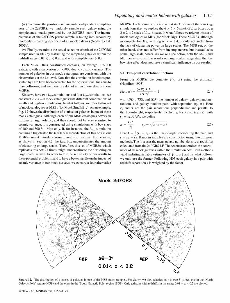
Since we have two L100 simulations and four L300 simulations, weconstruct 2 × 4 = 8 mock catalogues with different combinations ofsmall- and big-box simulations. In what follows, we refer to this setof mock catalogues as MSBs (for Mock Small/Big). As an example,Fig. 12 shows the distribution of a subset of galaxies in one of thesemock catalogues. Although each of our MSB catalogues covers anextremely large volume, and thus should not be very sensitive tocosmic variance, it is constructed using simulations with box sizesof 100 and 300 h−1 Mpc only. If, for instance, the L100 simulationcontains a big cluster, the 6 × 6 × 6 reproduction of this box in ourMGRSs might introduce some unrealistic features. Furthermore,as shown in Section 4.2, the L100 box underestimates the amountof clustering on large scales. Therefore, this set of MGRSs, whichreplicates this box 27 times, might underestimate the clustering onlarge scales as well. In order to test the sensitivity of our results tothese potential problems, and to have a better handle on the impact ofcosmic variance in our mock surveys, we construct four alternative

Figure 12. The distribution of a subset of galaxies in one of the MSB mock samples. For clarity, we plot galaxies only in two 3◦ slices, one in the ‘NorthGalactic Pole’ region (NGP) and the other in the ‘South Galactic Pole’ region (SGP). Only galaxies with redshifts in the range 0.01 < z < 0.2 are plotted.

MGRSs. Each consists of a 4 × 4 × 4 stack of one of the four L300

simulations (i.e. we replace the 6 × 6 × 6 stack of L100 boxes by a2 × 2 × 2 stack of L300 boxes). In what follows we refer to this set ofmock catalogues as MBs (for Mock Big). These MGRSs, althoughincomplete for M bJ − 5 log h > −18.4, should not suffer fromthe lack of clustering power on large scales. The MSB set, on theother hand, does not suffer from incompleteness, but instead lackssome large-scale power. As we will see below, both the MSB andMB mocks give similar results on large scales, suggesting that thebox-size effect does not have a significant influence on our results.

5.1 Two-point correlation functions

From our MGRSs we compute ξ (rp, π ) using the estimator(Hamilton 1993)

ξ (rp, π ) = 〈R R〉〈DD〉〈DR〉2

− 1 (24)

with 〈DD〉, 〈RR〉, and 〈DR〉 the number of galaxy–galaxy, random–random, and galaxy–random pairs with separation (rp, π ). Hererp and π are the pair separations perpendicular and parallel tothe line-of-sight, respectively. Explicitly, for a pair (s1, s2), withsi = czi r i/H0, we define

π = s · l|l| , rp =

√s · s − π 2 (25)

Here l = 12 (s1 + s2) is the line-of-sight intersecting the pair, and

s = s 1 − s 2. Random samples are constructed using two differentmethods. The first uses the mean galaxy number density at redshift zcalculated from the 2dFGRS LF. The second randomizes the coordi-nates of all mock galaxies within the simulation box. Both methodsyield indistinguishable estimates of ξ (rp, π ) and in what followswe only use the former. Following H03 each galaxy in a pair withredshift separation s is weighted by the factor

C© 2004 RAS, MNRAS 350, 1153–1173

1166 X. Yang et al.

Figure 13. The upper panels show the projected 2PCFs wp(rp)/rp for galaxies of different luminosity and type. The error bars correspond to the 1σ varianceamong distinct MGRSs (i.e. among the eight MSBs for the faintest subsamples, and among the four MBs for the brightest subsamples). For clarity, the errorbars are only plotted for the brightest and faintest subsamples. The lower panels plot the ratios of these wp(rp) to that of a reference sample. The referencesample contains all galaxies within the magnitude range −19.5 > M ′

bJ> −20.5 (with M ′

bJ= M bJ − 5 log h). Note that the faintest subsamples, which are

impacted by the box-size effect of the L100 simulation, reveal a ‘break’ at rp � 10 h−1 Mpc.

wi = 1

1 + 4πn(zi )J3(s)(26)

with n(z) the number density distribution as a function of redshiftand J3(s) = ∫ s

0ξ (s ′)s ′2 ds ′. Hence each galaxy–galaxy, random–

random, and galaxy–random pair is given a weight w iw j . We re-place ξ (s′) with a power law using the same parameters as in H03.This redshift-dependent weighting scheme is designed to minimizethe variance on the estimated correlation function (Davis & Huchra1982; Hamilton 1993).

Since the redshift-space distortions only affect π , the projectionof ξ (rp, π ) along the π -axis can get rid of these distortions and givea function that is more closely related to the real-space correlationfunction. In fact, this projected 2PCF is related to the real-space2PCF through a simple Abel transform

wp(rp) =∫ ∞

−∞ξ (rp, π ) dπ = 2

∫ ∞

r p

ξ (r )r dr√r 2 − r 2

p

(27)

(Davis & Peebles 1983). Therefore, if the real-space 2PCF is a powerlaw, ξ (r ) = (r 0/r )γ , the projected 2PCF w(rp) can be written as

wp(rp) = √π

�(γ /2 − 1/2)

�(γ /2)

(r0

rp

)γ

rp. (28)

We start our investigation of the redshift-space clustering prop-erties by computing wp(rp) for a number of luminosity bins and forearly- and late-type galaxies separately. To compare these projectedcorrelation functions with the 2dFGRS results from Norberg et al.(2002a), we estimate wp(rp) using volume-limited samples with thesame redshift and magnitude selection criteria as those adopted byNorberg et al. (2002a). For the MSB mocks (which use a stack of6 × 6 × 6 L 100 boxes), however, these wp(rp) reveal a systematic‘break’ at rp ∼ 10 h−1 Mpc. As we have shown in Section 4.2, thisis due to the fact that, because of the small box size of the L100

simulation, the 2PCF is too small on large scales (see Figs 6 and 7).We can circumvent this problem by using MGRSs from the MB set,in which the stack of 6 × 6 × 6 L 100 boxes is replaced by a stack of2 × 2 × 2 L 300 boxes. However, these MGRSs are only completedown to M bJ − 5 log h � −18.4 and can therefore only be used forgalaxies brighter than this.

The upper panels of Fig. 13 plot wp(rp) for different magnitudebins and for early- and late-type galaxies separately. Except forthe faintest magnitude bin, these projected correlation functions areobtained from MGRS in the MB set. Results for the magnitude binwith −17.5 > M bJ − 5 log h > −18.5 (solid lines) are obtained fromthe MSB set. As discussed in Paper II, the projection significantlywashes out the features in the real-space 2PCFs at ∼2 h−1 Mpc, andthe projected 2PCFs better resemble a power law. The exception isthe wp(rp) for the faintest subsample of galaxies, where the ‘break’mentioned above is clearly visible. To highlight the luminosity andtype dependence of wp(rp), the lower panels of Fig. 13 plot theratios of wp(rp) to that of a reference sample defined as all (early-type plus late-type) galaxies with −19.5 > M bJ − 5 log h > − 20.5.For a given luminosity, the correlation amplitude is higher, and theslope is steeper for early-type galaxies than for late-type galaxies.Significant changes in the slope (and thus deviations from a perfectpower law) occur at separations rp ∼ 2 h−1 Mpc, which is at leastqualitatively in agreement with recent results from the SDSS (Zehaviet al. 2003).

In order to facilitate a more direct comparison with the 2dF-GRS data, we fit a single power-law relation of the form (28) tothese wp(rp) over the range 2 h−1 Mpc < rp < 15 h−1 Mpc. Thisrange is also adopted by Norberg et al. (2002a) when fitting theprojected 2PCFs obtained from the 2dFGRS. Fig. 14 plots thereal-space correlation lengths r0 and the slopes γ thus obtainedas a function of luminosity and galaxy type. The agreement be-tween our MGRSs and the 2dFGRS is acceptable. The slight but

C© 2004 RAS, MNRAS 350, 1153–1173


Figure 14. The correlation lengths, r0, and slopes, γ , of the power laws that best fit the projected correlation functions over the range 2 � rp � 15 h−1 Mpc(solid squares). The results for the two faintest luminosity bins are based on the mean and variance of the sample of eight MSB mocks, while results for theother bins are based on the mean and variance of the sample of four MB mocks. Open circles with error bars correspond to the 2dFGRS data of Norberg et al.(2002a), and are shown for comparison. Except for a systematic overestimate of the correlation lengths, the cause of which has been discussed in Section 4.2,there is good agreement between our MGRSs and the 2dFGRS.

systematic overestimate of r0 is due to the effects discussed inSection 4.2.

We now turn to a comparison of the projected correlation functionfor the entire, flux limited surveys. The upper-left panel of Fig. 15compares the wp(rp) obtained from our eight MSB and four MBMGRSs with that of the 2dFGRS obtained by H03. The projectedcorrelation functions from our MSBs and MBs agree well with eachother (i.e. the 1σ error bars overlap), and, at rp � 3 h−1 Mpc, with the2dFGRS results. Note that at rp � 10 h−1 Mpc the w p(r p) obtainedfrom the MB mocks is slightly larger than that obtained from theMSB mocks, again due to the effects discussed in Section 4.2.

At large scales, wp(rp) is predominantly sensitive to the halo oc-cupation numbers 〈N(M)〉 and virtually independent of the secondmoment of P(N | M) or of details regarding the spatial distribution ofsatellite galaxies. The good agreement at large scales among differ-ent MGRSs and with the observations therefore strongly supportsour CLF and it shows that any ‘cosmic variance’ among the dif-ferent MGRSs has only a relatively small impact on wp(rp). Onsmall scales, however, the MGRSs reveal more correlation power(by about a factor 2) than observed. On such scales, wp(rp) is sensi-tive to our assumptions about the second moment of P(N | M) and, toa lesser degree, the spatial distribution of satellite galaxies. We shallreturn to this small-scale mismatch and its implications in Section 6below.

Rather than projecting ξ (rp, π ), one may also average ξ (rp, π )along constant s = √

r 2p + π 2, yielding the redshift-space 2PCFs

ξ (s). The upper-right panel of Fig. 15 plots ξ (s) obtained from ourMGRSs, compared to the 2dFGRS results from H03. We find sim-ilar behaviour as with the projected correlation function; the eightMSBs and four MBs agree quite well with each other and withthe observations at s � 6 h−1 Mpc. At smaller redshift-space sep-arations, however, the MGRSs slightly overpredict the correlation

power. Note that the MB samples predict higher ξ (s) on small scalesthan the MSB samples. This difference comes from the fact that theMB samples are incomplete for galaxies fainter than M bJ− 5 log h =−18.4. To test this we construct a mock survey from the MSB sam-ple, but only accepting galaxies brighter than this. This yields a ξ (s)in excellent agreement with that of the MB samples over all scales.Thus, although the use of only large-box simulations can result insystematic errors on small scale, the use of small-box simulations inthe MSB samples does not cause any significant, systematic errorson large scale.

5.2 Redshift-space distortions

We now turn to a comparison of the detailed shape of ξ (rp, π ).In particular, we focus on the distortions with respect to the real-space correlation function ξ (r) induced by the peculiar velocities ofgalaxies.

The two-dimensional correlation function ξ (rp, π ) is often mod-elled as a convolution of the real-space 2PCF ξ (r) and the conditionaldistribution function f (v12 | r):

1 + ξ (rp, π )

=∫ ∞

−∞

[1 + ξ

(√r 2

p + (π − v12/H0)2)]

f (v12 | r ) dv12 (29)

(Peebles 1980). Here v12 corresponds to the pairwise peculiar ve-locity along the line-of-sight and r corresponds to the real-spaceseparation. It is standard practice to assume an exponential form forf (v12| r) and to ignore its dependence on separation r (cf. Davis &Peebles 1983; Mo et al. 1993, 1997; Fisher et al. 1994; Marzke et al.1995; Guzzo et al. 1997; Jing et al. 2002; Zehavi et al. 2002). How-ever, as we have shown in Section 4, the exponential form is only

C© 2004 RAS, MNRAS 350, 1153–1173

1168 X. Yang et al.

Figure 15. The projected correlation function wp(rp) (top-left panel), the redshift-space correlation function ξ (s) (top-right), the quadrupole-to-monopoleratio q(s) (bottom-left), and the PVDs (bottom-right) for the samples of MSB (solid lines) and MB (dashed lines) surveys. Error bars, which are similar for MBand MSB results, are only shown for the MSB results for clarity. These error bars are based on the variance of the eight MSB surveys. The open circles witherror bars correspond to the 2dFGRS results obtained by Hawkins et al. (2003), and are shown for comparison. Note that the MSBs and MBs give approximatelythe same results, but that there are marked differences between model predictions and observations. Note also that the model error bars are in general largerthan the difference in the mean between MB and MSB results, implying that these error bars are statistical.

adequate at small separations, and the PVD varies quite strongly withseparation. Furthermore, equation (29) is only valid for an isotropicvelocity field in the limit where the probability of a real-space pairseparation r is independent of the probability of an associated rel-ative velocity v12. Although perhaps a reasonable approximationon small, highly non-linear, scales, it is certainly not valid in lin-ear theory where the velocity and density fields are tightly coupled.In an attempt to partially correct for this, one often assumes thatf (v12) is the probability distribution for the relative velocity aboutthe mean. Using the self-similar infall model, this mean pairwisepeculiar velocity, 〈v12〉, is modelled as

〈v12〉(r ) = −H0 F

(y

1 + (r/r0)2

)(30)

(Davis & Peebles 1977) with y = |π − v12/H 0| the separation inreal-space along the line-of-sight. F = 0 corresponds to a universewithout any flow other than the Hubble expansion, while F = 1corresponds to stable clustering. Given the fairly ad hoc nature ofthis model, and the strong sensitivity to the uncertain value of F(Davis & Peebles 1983), great care is required when interpretingany results based on this model.

A more robust model is based on linear theory and directly mod-elling the infall velocities around density perturbations. FollowingKaiser (1987) and Hamilton (1992) one can write the observed cor-relation function on linear scales as

ξlin(rp, π ) = ξ0(s)P0(µ) + ξ2(s)P2(µ) + ξ4(s)P4(µ). (31)

Here Pl (µ) is the lth Legendre polynomial, and µ is the cosine ofthe angle between the line-of-sight and the redshift-space separations. According to linear perturbation theory the angular moments canbe written as

ξ0(s) =(

1 + 2β

3+ β2

5

)ξ (r ), (32)

ξ2(s) =(

4β

3+ 4β2

7

)[ξ (r ) − ξ (r )

], (33)

ξ4(s) = 8β2

35

[ξ (r ) + 5

2ξ (r ) − 7

2ξ (r )

], (34)

with

ξ (r ) = 3

r 3

∫ r

0

ξ (r ′)r ′2 dr ′, (35)

C© 2004 RAS, MNRAS 350, 1153–1173


and

ξ (r ) = 5

r 5

∫ r

0

ξ (r ′)r ′4 dr ′. (36)

Given a value for β and the real-space correlation function, whichcan be obtained from ξ (rp, π ) via the projected correlation functionw p(r p), equation (31) yields a model for ξ (rp, π ) on linear scalesthat takes proper account of the coupling between the density andvelocity fields. To model the non-linear virialized motions of galax-ies within dark matter haloes, one convolves this ξ lin(rp, π ) with thedistribution function of pairwise peculiar velocities f (v12 | r).

1 + ξ (rp, π ) =∫ ∞

−∞[1 + ξlin(rp, π − v12/H0)] f (v12 | r ) dv12. (37)

Thus, by modelling ξ (rp, π ) one can hope to get both an es-timate of β as well as information regarding the pairwise peculiarvelocity distribution. We follow H03, and assume that the real-space2PCF is a pure power law, ξ (r ) = (r/r 0)−γ , and that f (v12 | r) is anexponential that is independent of the real-space separation r:

f (v12 | r ) = f (v12) = 1√2σ12

exp

(−

√2|v12|σ12

). (38)

Using a simple χ 2 minimization technique, we fit these models,described by the four parameters β, σ 12, r 0, and γ , to the ξ (rp, π )in each of our eight MSB and four MB MGRSs. The χ 2 is definedas

χ 2 =∑(

log[1 + ξ ]model − log[1 + ξ ]data

log[1 + ξ + �ξ ]data − log[1 + ξ − �ξ ]data

)2

, (39)

where the summation is over the ξ (rp, π ) data grid with the restric-tion 8 h−1 Mpc < s < 20 h−1 Mpc (see H03) and �ξ (rp, π ) is therms of ξ (rp, π ) determined from each of our eight MSB MGRSs(or of our four MB MGRSs). The averages (over the eight or thefour MGRSs) of the best-fitting values for β, σ 12, r 0, and γ , alongwith the variances among different samples, are listed in the firsttwo lines of Table 1. These should be compared with the valueslisted in the last line, which correspond to the best-fitting valuesobtained from the 2dFGRS by H03 using exactly the same method.As one can see, the best-fitting values for β and correlation lengthsof the MSB and the MB sample agree with each other and with the2dFGRS value at better than the 1σ level. On the other hand, thediscrepancies regarding γ and σ 12 are significant, both of which aresignificantly higher in our MGRSs than in the 2dFGRS.

In order to investigate these discrepancies in more detail we com-pute two statistics of the redshift space distortions which we com-pare to the 2dFGRS. As above, we take great care in using exactlythe same method and assumptions as H03. Therefore, even if someaspects of the model are questionable, this allows a meaningful com-parison of our results with those obtained by H03. First of all, wecompute the modified quadrupole-to-monopole ratio

q(s) ≡ ξ2(s)3s3

∫ s

0ξ0(s ′)s ′2 ds ′ − ξ0(s)

. (40)

where ξ l(s) is given by

ξl (s) = 2l + 1

2

∫ 1

−1

ξ (rp, π )Pl (µ) dµ. (41)

The lower-left panel of Fig. 15 plots q(s) for MSBs and MBs togetherwith the 2dFGRS results (open circles with error bars). Althoughthe MGRSs reveal the same overall behaviour as the 2dFGRS data,and are mutually consistent, they systematically overpredict q(s).

Table 1. Best-fitting parameters.

Survey β r0 γ σ 12

(1) (2) (3) (4) (5)

MSBs 0.52 ± 0.05 5.78 ± 0.23 1.99 ± 0.03 687 ± 37MBs 0.56 ± 0.06 5.93 ± 0.27 1.95 ± 0.03 732 ± 33(M/L)cl 0.52 ± 0.08 4.96 ± 0.21 1.88 ± 0.05 487 ± 44bvel 0.47 ± 0.06 5.99 ± 0.19 2.00 ± 0.06 497 ± 47σ 8 0.51 ± 0.06 5.19 ± 0.17 1.91 ± 0.05 505 ± 252dFGRS 0.49 ± 0.09 5.80 ± 0.25 1.78 ± 0.06 514 ± 31

The values of β, r0 (in h−1 Mpc), γ and σ 12 (in km s−1) that best fitthe ξ (rp, π ) for 8 h−1 Mpc < s < 20 h−1 Mpc for a number of differentMGRSs. Note that four MGRSs are used for MBs, while eight MGRSs areused for all other cases. The quoted values are the mean and 1σ variance ofthese MGRSs. The MGRSs denoted by ‘(M/L)cl’ are similar to the MGRSsin the MSB set, except that here the CLF is constrained to mass-to-lightratios for clusters of (M/L)cl = 1000 h (M/L)�, rather than (M/L)cl

= 500 h (M/L)� as in MSB (see Section 6.3). The MGRSs denoted by‘bvel’ are similar except for a velocity bias of bvel = σ gal/σ DM = 0.6 (seeSection 6.2). The MGRSs denoted by ‘σ 8’ are also similar except that theyadopt a flat �CDM cosmology with σ 8 = 0.75 rather than 0.9 (see Section6.4). The final line lists the best-fitting parameters obtained by Hawkinset al. (2003) by fitting the ξ (rp, π ) obtained from the 2dFGRS. Note that theerrors in Hawkins et al. are estimated from the spread of 22 Mock samples.

On small scales, where random peculiar velocities cause a rapidincrease of q(s), this indicates that the virialized motions in ourmock surveys are larger than observed (see also below). On largescales, where q(s) is asymptotic to the linear theory value of

q(s) = − 43 β − 4

7 β2

1 + 23 β + 1

5 β2, (42)

this might indicate that the value of β inherent to our MGRSs istoo small compared to the real Universe. On the other hand, Cole,Fisher & Weinberg (1994) have shown that non-linear, small-scalepower can affect q(s) out to fairly large separations. Therefore thesystematic overestimate of q at large s may simply be a reflectionof the random peculiar velocities being too large, rather than aninconsistency regarding the value of β.

The second statistic that we use to compare the redshift-spacedistortions in our MGRSs with those of the 2dFGRS are the PVDs,σ 12(rp), as a function of projected radius, rp. Following H03, wekeep r 0, γ and β fixed at the ‘global’ values listed in Table 1 anddetermine σ 12(rp) by minimizing χ2 in a number of independentrp bins.5 The results are shown in the lower-right panel of Fig. 15.Whereas the 2dFGRS reveals a σ 12(rp) that is almost constant withradius at about 500–600 km s−1, our MGRSs reveal a strong increasefrom σ 12 ∼ 600 km s−1 at rp = 0.1 h−1 Mpc to σ 12 ∼ 900 km s−1 atrp = 1.0 h−1 Mpc, followed by a decrease to σ 12 ∼ 500 km s−1 atrp = 10 h−1 Mpc. Thus, at around 1 h−1 Mpc, our MGRSs dra-matically overestimate the PVD. Although there is a non-negligibleamount of scatter among the different mock surveys, reflecting theextreme sensitivity of the PVDs to the few richest systems in the sur-vey, the variance among the eight (four) MGRSs is small comparedto the discrepancy.

As shown by Peacock et al. (2001) the best-fitting values of σ 12

and β are highly degenerate. We have tested the impact of this

5 Note that the PVDs thus obtained are a kind of average of the true PVDalong the line-of-sight. Therefore, these PVDs should not be compareddirectly to the true PVD shown in Fig. 9.

C© 2004 RAS, MNRAS 350, 1153–1173

1170 X. Yang et al.

degeneracy on our σ 12(rp) by repeating the same exercise using avalue for β that is 0.1 larger (smaller) than the values listed in Table1. This leads to an increase (decrease) of σ 12(rp) of the order of5 per cent (20 per cent) at projected radii of 1 h−1 Mpc (10 h−1

Mpc). Given that our MGRSs overpredict the PVD at rp = 1 h−1

Mpc by about 70 per cent, it is clear that this discrepancy is nota reflection of the β–σ 12 degeneracy. Thus, the standard �CDMmodel seems to have a severe problem in matching the observedPVDs on intermediate scales.

6 TOWA R D S A S E L F - C O N S I S T E N T M O D E LF O R L A R G E - S C A L E S T RU C T U R E

Our MGRSs, based on a flat �CDM concordance cosmology with�m = 0.3 and σ 8 = 0.9, and on a CLF that is required to yield clustermass-to-light ratios of (M/L)cl = 500 h (M/L)�, reveal clusteringstatistics that are overall in reasonable agreement with the data fromthe 2dFGRS. Nevertheless, two discrepancies have come to light:the MGRSs predict too much power on small scales and PVDs thatare too high. We now investigate possible ways to alleviate thesediscrepancies.

6.1 Halo occupation models

The discrepancies between our MGRS and the 2dFGRS resultsmight indicate a problem with our halo occupation models. Al-though the CLF is fairly well constrained by the observed luminosityfunction and the observed luminosity dependence of the correlationlengths (see Papers I and II), we have made additional assumptionsregarding the second moments of the halo occupation number distri-butions and regarding the distribution of galaxies within individualdark matter haloes.

As we have shown in Section 4.2 the real space correlation func-tion depends only very weakly on our method of distributing satellitegalaxies within dark matter haloes (cf. Fig. 8). We have verified, us-ing a number of tests, that modifications of the spatial distributionof satellite galaxies within dark matter haloes have no significantinfluence on wp(rp) or on σ 12(rp). Therefore, none of the discrep-ancies mentioned above can be attributed to errors in our satellitemodel.

Our results are more susceptible to changes in the second momentof the halo occupation number distributions. On small scales, ξ (r)scales with the average number of galaxy pairs in individual haloes〈 1

2 N (N −1)〉. Therefore, one can decrease the power on small scales,to bring our wp(rp) into better agreement with observations, bylowering the second moments of our halo occupation distributions.However, our distribution (16) is already the narrowest distributionpossible, and modifying the second moment of the halo occupationdistributions can therefore only aggravate the discrepancies on smallscales.

6.2 Velocity bias

A seemingly obvious explanation for the too-high PVDs is that thepeculiar velocities of galaxies are biased with respect to the darkmatter. We define the velocity bias (sometimes called ‘dynamical’bias) as bvel = σ gal/σ DM, with σ gal and σ DM the peculiar velocitydispersions of (satellite) galaxies and dark matter particles in a givenhalo, respectively. Note that in our fiducial MGRSs we adopt bvel = 1(i.e. no velocity bias). Fig. 16 shows w p(r p), ξ (s), q(s) and σ 12(rp)for MGRSs (with the MSB configuration of simulation boxes) inwhich bvel = 0.6; i.e. the velocity dispersion of satellite galaxies is

only 60 per cent of that of the dark matter particles in the same halo(dashed lines). With such a pronounced velocity bias, both q(s) andthe PVDs, as well as β and the global value of σ 12 listed in Table 1,are all consistent with the 2dFGRS results.

In two recent papers, Berlind et al. (2003) and Yoshikawa et al.(2003) measured the velocity bias of ‘galaxies’ in a smoothed parti-cle hydrodynamics (SPH) simulation and found that bvel decreasesfrom bvel ∼ 0.9–1.0 for haloes with M ∼ 3 × 1014 h−1 M� to bvel

∼ 0.6–0.8 for haloes with M ∼ 3 × 1012 h−1 M�. Thus, althoughsimulations predict that low-mass haloes might have values for thevelocity bias as low as bvel � 0.6, required here to bring our PVDsin agreement with observations, the PVD is dominated by galax-ies in massive haloes for which these same simulations apparentlypredict close to bvel = 1 (i.e. no velocity bias). Furthermore, the in-troduction of velocity bias cannot solve the excess power on smallscales. After all, the real-space correlation function is independentof bvel such that the discrepancies regarding wp(rp) on small scalesremain (see upper-left panel of Fig. 16). To make matters worse, re-ducing the peculiar velocities of galaxies inside dark matter haloes,increases the small-scale power in redshift space. This means thatthe redshift-space correlation function ξ (s) actually becomes morediscrepant with the 2dFGRS data (see upper-right panel of Fig. 16).Therefore, although a certain amount of velocity bias might be ex-pected, we do not consider it a viable solution for the problemsmentioned above.

6.3 Cluster mass-to-light ratios

Because the PVD is a pair-weighted statistic it is extremely sensitiveto the few richest systems in the sample (i.e. Mo, Jing & Borner 1993,1997; Zurek et al. 1994; Marzke et al. 1995; Somerville, Primack& Nolthenius 1997). The fact that the PVDs in our MGRSs aretoo large compared with observations therefore might indicate thateither there are too many clusters of galaxies in our mock surveys(see Section 6.4 below), or that these clusters contain too manygalaxies.

Our CLF was constructed under the constraint that the averagemass-to-light ratio of haloes with M � 1014 h−1 M� is equal to(M/L)cl = 500 h (M/L)� (in the photometric bJ band). This valueis motivated by the average mass-to-light ratio of clusters obtainedby Fukugita, Hogan & Peebles (1998). To reduce the number ofgalaxies per cluster we now set (M/L)cl = 1000 h (M/L)� andrepeat the entire exercise: we first use the method described in Sec-tion 2 to compute the parameters of the new conditional luminosityfunction. This CLF is used to construct new MGRSs (using thesame configuration of simulation boxes as in MSB), from which wedetermine the same statistics as before.

The results are listed in Table 1 and shown as dotted lines inFig. 16. Clearly, increasing the mass-to-light ratio of clusters low-ers q(s) and σ 12(rp), bringing them into better agreement with the2dFGRS results. Although the PVDs are still somewhat too high,especially at around ∼0.4 h−1 Mpc, the extent of this discrepancyis similar to its 1σ variance of the eight MGRSs, indicating thatthis remaining difference is consistent with ‘cosmic variance’. Ascan be seen from Table 1, both β and γ are now in much betteragreement with the 2dFGRS. In addition, the reduction of the num-ber of galaxies in clusters significantly reduces wp(rp) at small pro-jected separations (see Fig. 16), bringing it into good agreement withthe observations.6 A similar reduction of small-scale power is also

6 Note that the correlation amplitude predicted with (M/L)cl = 1000

C© 2004 RAS, MNRAS 350, 1153–1173


Figure 16. Same as Fig. 15 except that here we compare the results for the MSB sample with those of three alternative MGRSs in which we have modifiedthe CLF to yield cluster mass-to-light ratios of (M/L)cl = 1000 h (M/L)� (dotted lines), in which we adopt a velocity bias of bvel = 0.6 (dashed lines), andin which we adopt a cosmology with σ 8 = 0.75 (dot-dashed lines). All results correspond to the mean of the entire sample of eight MSB mock surveys. Forclarity, no error bars are plotted here, but they are similar to those shown in Fig. 15. Note that both the (M/L)cl = 1000 h (M/L)� model and the σ 8 = 0.75model are in good agreement with the observational data.

evident in ξ (s). Thus, these particular MGRSs have clustering char-acteristics that are overall in good agreement with the 2dFGRS re-sults. The question is therefore whether or not such a high mass-to-light ratio for clusters of galaxies is compatible with observations.

The cluster mass-to-light ratios quoted by Fukugita et al. (1998)are (450 ± 100) h (M/L)� in the B-band based on X-ray andvelocity-dispersion data. Taking these numbers at face value, acluster mass-to-light ratio of (M/L)cl = 1000 h (M/L)� is ruledout at the 5σ level. Using a variety of methods to estimate clus-ter masses, Bahcall et al. (2000) obtained (M/L)B = (330 ± 77)h (M/L)�, which is consistent with the results of Carlberg et al.(1996), (M/L)B = (363 ± 65) h (M/L)�, based on galaxy kine-matics in clusters. Taking the average of these two measurementsyields 〈M/LB〉cl = (350 ± 70) h (M/L)�, which rules out the clustermass-to-light ratio required to match the clustering power on smallscales at more than 7σ . Thus, unless the cluster mass-to-light ratios

h(M/L)� is slightly lower than the observed amplitude, because in thismodel more galaxies are assigned to small haloes in order to match the ob-served luminosity function. Since the error bars on the observed correlationlengths are relatively large, the model tends to compromise the accuracy ofthe fit to the correlation lengths.

obtained from current observations are seriously in error, increasingthe average cluster mass-to-light ratio to (M/L)cl � 1000 h (M/L)�does not seem a viable solution for the problems at hand.

6.4 Power-spectrum normalization

Rather than lowering the average number of galaxies per cluster, wemay also hope to lower the PVDs by reducing the actual number ofclusters. As we have shown in Section 5.2, our results, and thus thenumber density of rich clusters, is robust against cosmic variance.Therefore, a lower number density of clusters implies a differentcosmological model. It is well known that the abundance of (rich)clusters is extremely sensitive to the power-spectrum normalizationparameter σ 8. The too-high PVDs could thus be indicative of atoo-high value for σ 8.

We therefore wish to compute the PVDs in a �CDM cosmol-ogy with identical cosmological parameters as before, except thatσ 8 = 0.75 rather than 0.9. Note that the choice of σ 8 = 0.75 issomewhat arbitrary, but it does represent a compromise between theconstraints on the value of σ 8 from various observations and the lowvalue required by our results on the PVDs (see below). In principle,constructing new MGRSs for a different cosmology requires new

C© 2004 RAS, MNRAS 350, 1153–1173

1172 X. Yang et al.

N-body simulations of the dark matter distribution. This, however, iscomputationally too expensive, which is why we use an approximatemethod instead. First, we compute the new best-fitting parametersof the CLF for this cosmology, again demanding that (M/L)cl =500 h (M/L)�. Next we populate the dark matter haloes in ourσ 8 = 0.9 simulation boxes with galaxies according to this new CLF.Finally, we construct a new sample of eight MSB MGRSs, in whichwe weigh each galaxy in a halo of mass M by

w = n(M | σ8 = 0.75)

n(M | σ8 = 0.9)(43)

with n(M) the number density of dark matter haloes of mass M. This,to first order, mimics the effect of lowering σ 8 on the halo massfunction, and so should be a reasonable approximation on smallscales where the clustering properties are determined by the galaxydistribution in individual haloes.7 The results for these MGRSs areshown as dot-dashed lines in Fig. 16. As one can see, the agreementwith observational results in this model is much better than in thestandard �CDM model. These results suggest that a �CDM modelwith σ 8 ∼ 0.75 may match all the observational results obtainedfrom the 2dFGRS. Unfortunately, in the absence of proper N-bodysimulations for this model, it is impossible to make a more detailedcomparison with observation.

The question is, of course, whether such a low σ 8 is compatiblewith other independent observations. Currently, the value of σ 8 isconstrained mainly by three types of observations: weak lensingsurveys, cluster mass functions, and anisotropy in the cosmic mi-crowave background. Recent cluster abundance analyses give valuesof σ 8 (assuming �m = 0.3) in a wide range, from 0.6 to 1 (e.g. Fan &Bahcall 1998; Pen 1998; Borgani et al. 2001; Reiprich & Bohringer2002; Seljak 2002; Viana, Nichol & Liddle 2002). Results fromweak-lensing surveys are equally uncertain, with σ 8 spanning therange 0.7 to ∼1 (e.g. Hoekstra, Yee & Gladders 2002; Refregier,Rhodes & Groth 2002; Bacon et al. 2003; Jarvis et al. 2003). Thus,our preferred value, σ 8 = 0.75, is consistent with these observations.At the moment, the most stringent constraint on the value of σ 8 isfrom WMAP (Spergel et al. 2003): σ 8 = 0.84 ± 0.04 (1σ error).Even taking this result at face value, one cannot rule out σ 8 = 0.75with any high confidence. Thus, there is no strong observationalevidence to argue against a �CDM model with σ 8 = 0.75. Further-more, as discussed by van den Bosch, Mo & Yang (2003b), a valueof σ 8 as low as 0.75 can also help to alleviate several problemsin current models of galaxy formation, such as those in connec-tion with the Tully–Fisher relation and to the rotation curve shapesof low-surface-brightness galaxies. Our results presented here giveadditional support for a relatively low value of σ 8.

7 C O N C L U S I O N S

In this paper, we have used realistic halo occupation distributions,obtained using the conditional luminosity function technique in-troduced by Yang et al. (2003), to populate dark matter haloes inhigh-resolution simulations of the �CDM ‘concordance’ cosmol-ogy. The simulations follow the evolution of 5123 dark matter par-ticles in periodic boxes of 100 h−1 Mpc and 300 h−1 Mpc on a side.Subsequently, the dark matter haloes identified in these simulations

7 Note that for haloes with a given mass, the concentration parameters aresmaller in the σ 8 = 0.75 model than they are in the standard �CDM model.This change of concentration is taken into account in our analyses, eventhough its effect is almost negligible.

are populated with galaxies of different luminosity and differentmorphological type.

We have shown that the luminosity functions and the correlationlengths as a function of luminosity, both for early- and late-typegalaxies, are in good agreement with observations. Since these sameobservations were used to constrain the conditional luminosity func-tions, which in turn were used to populate the dark matter haloes, thisagreement shows that the halo occupation statistics obtained ana-lytically can be implemented reliably in N-body simulations to con-struct realistic, self-consistent, mock galaxy distributions. We havedemonstrated that the details of the spatial distribution of galaxieswithin individual dark matter haloes have only a very mild effecton the two-point correlation function, and only at real-space sepa-rations r � 0.3 h−1 Mpc.

The mean pairwise peculiar velocities, 〈v12〉, however, dependrather strongly on whether satellite galaxies (any galaxy in a darkmatter halo other than the most luminous, central galaxy) are asso-ciated with random dark matter particles of the friends-of-friends(FOF) group, or whether they are assigned peculiar velocities as-suming a spherical, isotropic velocity distribution around the centralgalaxy. In the former case, 〈v12〉, which indicates the amount of in-fall around overdensity regions, is similar to that of the dark matter.In the latter case, 〈v12〉 is significantly suppressed with respect tothe dark matter. This difference indicates that the outer parts of theFOF-groups are not yet virialized.

The pairwise velocity dispersions (PVDs) of the galaxies arefound to be significantly smaller than those of dark matter parti-cles. Since the PVD is a pair-weighted measure for the potentialwell in which dark matter particles (galaxies) reside, this can beunderstood as long as the average number of galaxies per unit halomass, N/M, decreases with M (Jing et al. 1998). Indeed, the halo oc-cupation numbers inferred from our conditional luminosity functionindicate that N/M ∝ Ma with a ∼ −0.2.

Stacking a number of 100 h−1 Mpc and 300 h−1 Mpc simulationboxes allows us to construct mock galaxy redshift surveys (MGRSs)that are comparable to the 2dFGRS in terms of sky coverage, depthand magnitude limit. For each of these MGRSs we estimate thetwo-point correlation functions ξ (rp, π ). These are used to derivea number of statistics about the large-scale distribution of galaxies,which we compare directly with the 2dFGRS results. In particular,we calculate the projected 2PCFs wp(rp) as a function of luminosityand type. The best-fitting power-law slope and correlation lengths ofthese projected correlation functions are found in good agreementwith the 2dFGRS results obtained by Norberg et al. (2002a). Inaddition, we also compute wp(rp) and the redshift space correlationfunction ξ (s) for the entire MGRSs. These are compared to the2dFGRS results obtained by Hawkins et al. (2003).

Although the agreement with the 2dFGRS data is excellent onscales larger than ∼3 h−1 Mpc, on smaller scales wp(rp) is abouta factor of 2 larger than observed. To investigate this in more de-tail, we analysed the redshift-space distortions present in ξ (rp, π )by computing the quadrupole-to-monopole ratios q(s) and the pair-wise velocity dispersions σ 12(rp). A comparison with the results ofHawkins et al. (2003) shows that the standard �CDM model over-predicts the clustering power on small scales by a factor of about 2,and the PVDs by about 350 km s−1. After examining a variety ofpossibilities, we find that the only viable solution to these problemsis to reduce the power-spectrum amplitude, σ 8, from 0.9 to ∼0.75.

No doubt, in the coming years, new results from the 2dFGRSand the SDSS will significantly improve the data on the large-scaledistribution of galaxies. The analysis presented here, based on theconditional luminosity function, will hopefully prove a useful tool

C© 2004 RAS, MNRAS 350, 1153–1173


to further constrain both galaxy formation and cosmology. In thisrespect, our results regarding constraints on σ 8 are an importantillustration of the potential power of this approach.

AC K N OW L E D G M E N T S

We thank Ed Hawkins and the 2dFGRS team for providing us withtheir data in electronic format, the anonymous referee for insightfulcomments that helped to improve the paper, and Gerhard Borner,Guinevere Kauffmann, Simon White and Saleem Zaroubi for usefuldiscussions. XHY is supported by NSFC (No.10243005) and byUSTCQN. YPJ is supported in part by NKBRSF (G19990754) andby NSFC (No.10125314). Numerical simulations presented in thispaper were carried out at the Astronomical Data Analysis Centre(ADAC) of the National Astronomical Observatory, Japan.

R E F E R E N C E S

Bacon D., Massey R., Refregier A., Ellis R., 2003, MNRAS, 344, 673Bahcall N. A., Cen R., Dave R., Ostriker J. P., Yu Q., 2000, ApJ, 541, 1Benson A. J., Cole S., Frenk C. S., Baugh C. M., Lacey C. G., 2000, MNRAS,

311, 793Benson A. J., Baugh C. M., Cole S., Frenk C. S., Lacey C. G., 2002, MNRAS,

316, 107Berlind A. A., Weinberg D. H., 2002, ApJ, 575 587Berlind A. A. et al., 2003, ApJ, 593, 1Borgani S. et al., 2001, ApJ, 561, 13Bullock J. S., Kolatt T. S., Sigad Y., Somerville R. S., Klypin A. A., Primack

J. R., Dekel A., 2001, MNRAS, 321, 559Bullock J. S., Wechsler, R. H., Somerville R. S., 2002, MNRAS, 329, 246Bryan G., Norman M., 1998, ApJ, 495, 80Carlberg R. G., Yee H. K. C., Ellingson E., Abraham R., Gravel P., Morris

S., Pritchet C. J., 1996, ApJ, 462, 32Cole S., Fisher K. B., Weinberg D. H., 1994, MNRAS, 267, 785Cole S., Hatton S., Weinberg D. H., Frenk C. S., 1998, MNRAS, 300, 945Colless M. et al., 2001, MNRAS, 328, 1039Cooray A., Sheth R., 2002, Phys. Rep., 372, 1Diaferio A., Geller M. J., 1996, ApJ, 467, 19Davis M., Huchra J., 1982, ApJ, 254, 437Davis M., Peebles P. J. E., 1977, ApJS, 34, 425Davis M., Peebles P. J. E., 1983, ApJ, 267, 465Davis M., Efstathiou G., Frenk C. S., White S. D. M., 1985, ApJ, 292, 371Efstathiou G., Frenk C. S., White S. D. M., Davis M., 1988, MNRAS, 235,

715Fan X., Bahcall N. A., 1998, ApJ, 504, 1Fisher K. B., Davis M., Strauss M. A., Yahil A., Huchra J. P., 1994, MNRAS,

267, 927Fukugita M., Hogan C. J., Peebles P. J. E., 1998, ApJ, 503, 518Guzzo L., Strauss M. A., Fisher K. B., Giovanelli R., Haynes M. P., 1997,

ApJ, 489, 37Hamilton A. J. S., 1992, ApJ, 385, L5Hamilton A. J. S., 1993, ApJ, 417, 19Hawkins E. et al., 2003, MNRAS, 346, 78 (H03)Hoekstra H., Yee H. K. C., Gladders M. D., 2002, ApJ, 577, 595Huffenberger K. M., Seljak U., 2003, MNRAS, 340, 1199Jarvis M., Bernstein G. M., Fischer P., Smith D., Jain B., Tyson J. A., Wittman

D., 2003, AJ, 125, 1014Jing Y. P., Suto Y., 2002, ApJ, 574, 538

Jing Y. P., Borner G., Suto Y., 2002, ApJ, 564, 15Jing Y. P., Mo H. J., Borner G., 1998, ApJ, 494, 1Kaiser N., 1987, MNRAS, 227, 1Kang X., Jing Y. P., Mo H. J., Borner G., 2002, MNRAS, 336, 892Kauffmann G., Nusser A., Steinmetz M., 1997, MNRAS, 286, 795Kauffmann G., Colberg J. M., Diaferio A., White S. D. M., 1999, MNRAS,

303, 188Kochanek C. S., White M., Huchra J., Macri L., Jarrett T. H., Schneider S.

E., Mader J., 2003, ApJ, 585, 161Madgwick D. S. et al., 2002, MNRAS, 333, 133Magira H., Jing Y. P., Suto Y., 2000, ApJ, 528, 30Marinoni C., Hudson M. J., 2002, ApJ, 569, 101Marzke R. O., Geller M. J., Da Costa L. N., Huchra J. P., 1995, AJ, 110,

477Mathis H., Lemson G., Springel V., Kauffmann G., White S. D. M., Eldar

A., Dekel A., 2002, MNRAS, 333, 739Mo H. J., Jing Y. P., Borner G., 1993, MNRAS, 264, 825Mo H. J., Jing Y. P., Borner G., 1997, MNRAS, 286, 979Navarro J. F., Frenk C. S., White S. D. M., 1997, ApJ, 490, 493Norberg P. et al., 2002a, MNRAS, 332, 827Norberg P. et al., 2002b, MNRAS, 336, 907Peacock J. A., Smith R. E., 2000, MNRAS, 318, 1144Peacock J. A. et al., 2001, Nat, 410, 169Peebles P. J. E., 1980, The Large-Scale Structure of the Universe. Princeton

Univ. Press, PrincetonPen U.-L., 1998, ApJ, 498, 60Porciani C., Dekel A., Hoffman Y., 2002, MNRAS, 332, 325Reiprich T. H., Bohringer H., 2002, ApJ, 567, 716Refregier A., Rhodes J., Groth E. J., 2002, ApJ, 572, L131Regos E., Geller M. J., 1991, ApJ, 377, 14Scoccimarro R., Sheth R. K., Hui L., Jain B., 2001, ApJ, 546, 20Scranton R., 2002, MNRAS, 332, 697Seljak U., 2000, MNRAS, 318, 203Seljak U., 2002, MNRAS, 337, 769Seto N., Yokoyama J. I., 1998, ApJ, 492, 421Sheth R. K., 1996, MNRAS, 279, 1310Sheth R. K., Tormen G., 1999, MNRAS, 308, 119Sheth R. K., Mo H. J., Tormen G., 2001, MNRAS, 323, 1Smith R. E. et al., 2003, MNRAS, 341, 1311Somerville R. S., Primack J. R., Nolthenius R., 1997, ApJ, 479, 606Somerville R. S., Lemson G., Sigad Y., Dekel A., Kauffmann G., White

S. D. M., 2001, MNRAS, 320, 289Spergel D. N. et al., 2003, ApJS, 148, 175van den Bosch F. C., Yang X. H., Mo H. J., 2003a, MNRAS, 340, 771

(Paper II)van den Bosch F. C., Mo H. J., Yang X. H., 2003b, MNRAS, 345, 923van de Weygaert R., van Kampen E., 1993, MNRAS, 263, 481Viana P. P., Nichol R., Liddle A. R., 2002, ApJ, 569, L75White M., 2001, MNRAS, 321, 1Yang X. H., Mo H. J., van den Bosch F. C., 2003, MNRAS, 339, 1057

(Paper I)York D. et al., 2000, AJ, 120, 1579Yoshikawa K., Jing Y. P., Borner G., 2003, ApJ, 590, 654Zehavi I. et al., 2002, ApJ, 571, 172Zehavi I. et al., 2003, preprint (astro-ph/0301280)Zheng Z., Tinker J. L., Weinberg D. H., Berlind A. A., 2002, ApJ, 575, 617Zurek W., Quinn P. J., Salmon T. K., Warren M. S., 1994, ApJ, 431, 559

This paper has been typeset from a TEX/LATEX file prepared by the author.

C© 2004 RAS, MNRAS 350, 1153–1173

Populating dark matter haloes with galaxies: comparing the ...€¦ · (PVD) that are ∼400 km...

Documents

Transcript of Populating dark matter haloes with galaxies: comparing the ...€¦ · (PVD) that are ∼400 km...