POLYTECHNIC OF TORINO DEPARTMENT OF MECHANICAL ENGINEERING AND

AEROSPACE

MASTER THESIS Thermomechanical Characterization of Shape

Memory Alloy Wires

STUDENT: TEGUEFOUET ROMUAL DESIRE

SUPERVISORS: RAPARELLI TERENZIANO (DIMEAS)

MAFFIODO DANIELA (DIMEAS)

1 INTRODUCTION TO SHAPE MEMORY ALLOYS (SMA) .......................................... 1

1.1 General introduction ................................................................................................... 1 1.2 Motivation and Purpose of the study .......................................................................... 1

2 BACKGROUND ................................................................................................................ 2

2.1 What is unique about NiTi alloy? .............................................................................. 2 2.2 A Brief History of Shape Memory Alloys ................................................................. 3

2.2.1 Shape Memory Alloys and Common Metallic material ..................................... 3 2.3 Phenomenology of Phase Transformation in SMA .................................................... 4

2.3.1 NiTi B2 austenitic phase: ................................................................................... 4

2.3.2 NiTi B19' martensitic phase: .............................................................................. 4 2.3.3 NiTi R-phase ...................................................................................................... 6

2.4 Martensitic Phase Transformation in TiNi ................................................................. 6

3 Mechanical Behavior of TiNi ............................................................................................. 9 3.1 Shape Memory Effect ................................................................................................. 9 3.2 Superelasticity Effect ............................................................................................... 10 3.3 Stress-Strain Curve of Superelastic TiNi Alloy ....................................................... 10

3.4 Hysteresis in NiTi ..................................................................................................... 12 4 Review of Literature about SMA ..................................................................................... 12

4.1 Electrical Resistivity-Based Study of Self-Sensing ................................................. 12 4.1.1 Analysis of ER Properties of SMA Actuated AM ........................................... 13

4.1.2 Experimental Setup .......................................................................................... 13 4.1.3 Experimental Results ........................................................................................ 14

4.1.4 Experimental Results at Various Constant Stresses ......................................... 15

4.2 Feedback of Resistance ............................................................................................ 17

4.2.1 Open ring Test .................................................................................................. 17

5 Experiment ....................................................................................................................... 21

5.1 Description of the set-up .......................................................................................... 23 5.1.1 Climatic Chamber ............................................................................................ 23 5.1.2 VirtualBench VB8012-307E2EF NI ............................................................... 24

5.1.3 NI USB 6211 data acquisition .......................................................................... 24

5.1.4 Supports ............................................................................................................ 25 5.1.5 Computers ........................................................................................................ 26 5.1.6 Electrical connector .......................................................................................... 26 5.1.7 Sensor laser Model optoNCDT 1300 ............................................................... 28 5.1.8 Error made during the experimentation............................................................ 29

6 Procedure of experimentation .......................................................................................... 30 6.1 set-up and acquisition of the data of the measure .................................................... 31

6.1.1 Temperature ..................................................................................................... 31

6.1.2 Deformation (Strain recovery) ......................................................................... 36 6.1.3 Resistance ......................................................................................................... 40

7 Thermal Cycling Test ....................................................................................................... 41 7.1 Result and Interpretation .......................................................................................... 45

7.1.1 Thermo-mechanical cycle under constant load of 58,90 MPa ......................... 45 7.1.2 Thermo-mechanical test under constant load of 117MPa ................................ 47 7.1.3 Thermo-mechanical test under constant load of 176 MPa ............................... 50 7.1.4 Approximation of Linear equation between resistivity and the strain ............. 52

8 Discussion of the Results ................................................................................................. 54 9 Conclusion ........................................................................................................................ 56 10 Bibliographie .................................................................................................................... 58

1

1 INTRODUCTION TO SHAPE MEMORY ALLOYS (SMA)

1.1 General introduction

The critical advancement of material science needs the development and creation of new material science because generally, this is the precursor of many progressive innovations. Therefore, Shape memory alloys appear as the new solution materials, having some interesting characteristics such as superelasticity and shape memory, exploited through the interplay of structure and properties. They exist metallic alloys with more than two elements, exhibiting special characteristics. Two main families of SMA exist. – “copper-based” materials – Cu-Al (Zn, Ni, Be, etc.); – Nickel-Titanium-X materials (where X is an element present in small proportions) – NiTi (Fe, Cu, Co, etc.). What does ‘Memory’ mean? The term memory simply means that they have the property of ''remembering'' thermo-mechanical treatments to which they have been subjected, for example, torsion, traction flexion, etc.). In general, the geometry shape that they had at high and at low temperature constitutes two states that they remember. The training process is the way to give the memory to a material, by doing a certain number of repetition of thermodynamic process submitting the material to a cycle of stress, strain, and temperature. The key point for what they also call ‘Smart material’ is the phase transformation between parent phase called Austenitic (A) and the phase that is obtained after cooling called martensitic (M) [1]. In general, active materials has one or more properties that can be altered and this practically forms the basis of a smart structure and lead to the innovation application. Unless SMA is doped, is generally exhibits first-order transformation (high-temperature austenitic → low-temperature martensitic) involving a change in crystalline symmetry [2].

1.2 Motivation and Purpose of the study

Shape Memory Alloys (SMA) have been one of the most important fields of research during the last decades concerning materials science. In many fields, as

2

Robotic, Biomedical, aeronautic, aerospace and the nuclear industry, they became useful for several ranges of applications. The important thing is that the smart material is not useful just for their structural mechanical properties like toughness but they are also very interesting to play a function of sensor or actuator. SMA have electrical resistance characteristics which vary with phase transformations. The goal of this thesis is to understand how the electrical resistivity change with respect either the temperature or deformation. But in other to do this it is important to figure out some others characteristics of SMA regarding Shape Memory Effect, super elasticity, pseudoelasticity and phase transformation, etc. [1]

2 BACKGROUND

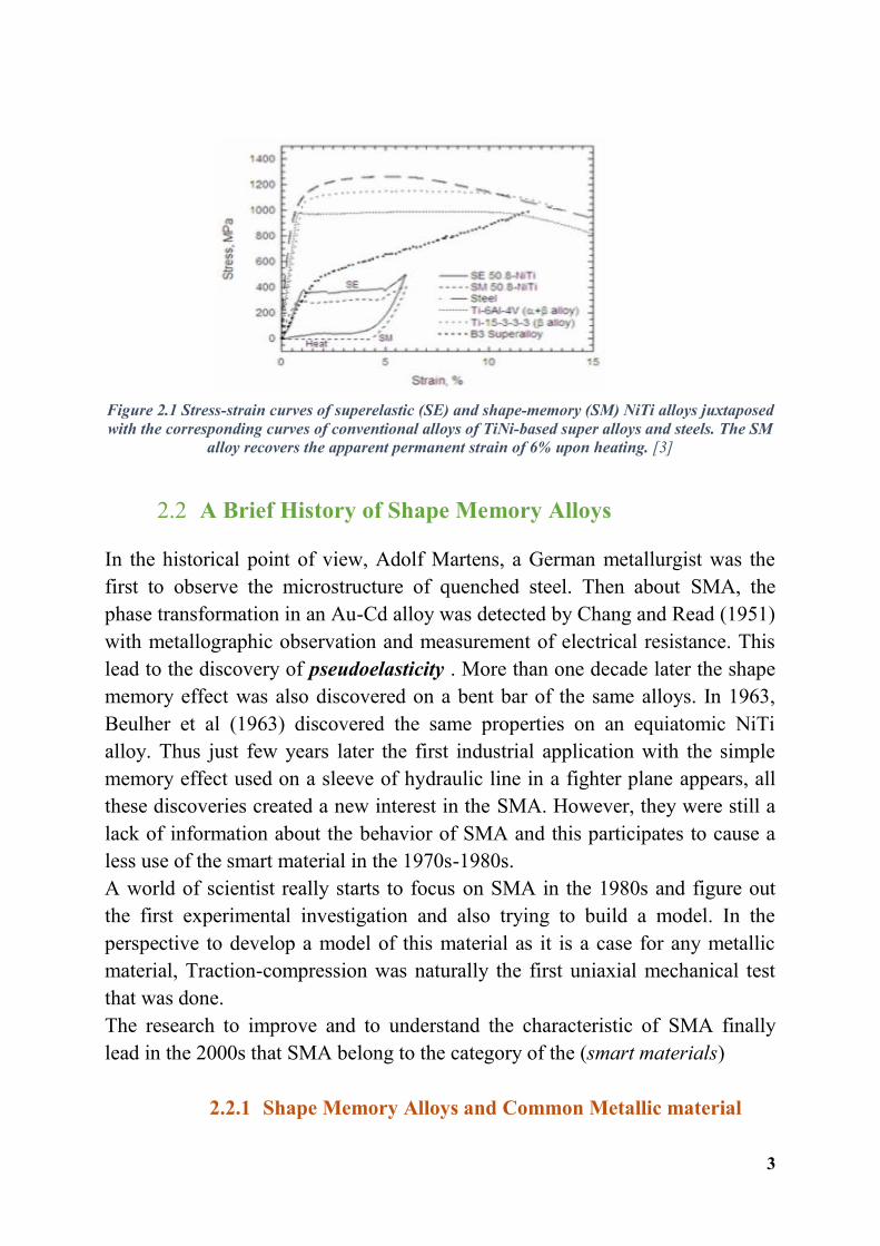
2.1 What is unique about NiTi alloy? The development of novel materials is critical for the advancement of materials engineering and is often the vanguard for many progressive innovative applications. NiTi is known as Nitinol for an engineering point of view because respect to other common material they have the capability to memorize their shape(s), this means that after a severe deformation (some percent) SMA can easily and spontaneously return to theirs predefine shape under some thermal condition. This property that exhibits SMA is termed Shape memory (SM), this occurs under thermal and mechanical conditions. SMA also exhibit another important property called superelasticity (SE). This second property has a particularity that allows to SMA to deforms to a very high strain (6 to 10%) and recovers the original predefine shape spontaneously whenever is unloaded. The physical manifestation of these two phenomena, SM and SE is observed in fig 2.1. [3]

3

Figure 2.1 Stress-strain curves of superelastic (SE) and shape-memory (SM) NiTi alloys juxtaposed with the corresponding curves of conventional alloys of TiNi-based super alloys and steels. The SM

alloy recovers the apparent permanent strain of 6% upon heating. [3]

2.2 A Brief History of Shape Memory Alloys

In the historical point of view, Adolf Martens, a German metallurgist was the first to observe the microstructure of quenched steel. Then about SMA, the phase transformation in an Au-Cd alloy was detected by Chang and Read (1951) with metallographic observation and measurement of electrical resistance. This lead to the discovery of pseudoelasticity . More than one decade later the shape memory effect was also discovered on a bent bar of the same alloys. In 1963, Beulher et al (1963) discovered the same properties on an equiatomic NiTi alloy. Thus just few years later the first industrial application with the simple memory effect used on a sleeve of hydraulic line in a fighter plane appears, all these discoveries created a new interest in the SMA. However, they were still a lack of information about the behavior of SMA and this participates to cause a less use of the smart material in the 1970s-1980s. A world of scientist really starts to focus on SMA in the 1980s and figure out the first experimental investigation and also trying to build a model. In the perspective to develop a model of this material as it is a case for any metallic material, Traction-compression was naturally the first uniaxial mechanical test that was done. The research to improve and to understand the characteristic of SMA finally lead in the 2000s that SMA belong to the category of the (smart materials)

2.2.1 Shape Memory Alloys and Common Metallic material

4

In general, common metallic material can’t undergo a limit of 0.2% of deformation if they speak about simple traction test, but SMA in reverse can undergo an extremely significant reversible deformation range, up to (6-7%), This is made possible by doing an important heat treatment. [1]

2.3 Phenomenology of Phase Transformation in SMA

2.3.1 NiTi B2 austenitic phase:

Austenitic is a high-temperature phase of TiNi as compare to martensitic phase and its crystal structure is cubic B2, figure 2.2. B2 has a lattice constant of 0.3015nm at room temperature. During slow cooling or quenching to room temperature, they retained its phase and this phase underwent the martensitic transformation and exhibit SM or SE effects. [3] [2].

Figure 2.2Austenitic, parent phase of TiNi [4]

2.3.2 NiTi B19' martensitic phase: Martensitic derives from the austenitic phase of NiTi and has a different crystal structure, it is a low-temperature phase of NiTi. Martensitic phase (B19, orthorhombic crystal structure) is less stable compared to Martensitic (B19') that is monoclinic crystal structure. Each of the following phase; monoclinic B19’ phase, orthorhombic B19 phase or trigonal R-phase is the martensitic transformations of Nitinol and NiTi, depending on the composition and the alloying elements they can have a different crystal structure. This type of transformation occurs due to shear lattice distortion (Kumar & Lagoudas, 2008). Figure 2.3 and figure 2.4 clearly highlight it. [2] [3]

5

Figure 2.3Crystal structure of B19 martensitic [4]

Figure 2.4Crystal structure of B19’ martensitic [4]

Let now introduce the term "Variants" which is the name given to the different orientation that has a crystal formed by the martensitic transformation. They are two forms of martensitic crystal: Twinned martensitic (figure 2.5) that is formed by the combination of "self-accommodation" martensitic variants (Kumar & Lagoudas, 2008) then Detwinned martensitic,(figure 2.6) in this case, is the reoriented martensitic variants that grow at the expense of other less favorable oriented variants. [5]

Figure 2.5 Twinned Martensitic [5]

6

Figure 2.6 Detwinned Martensitic [5]

2.3.3 NiTi R-phase During martensitic phase transformation, it is possible that the phase called R-phase occurs, but this happens before the B19' phase, and under some specific condition and has a trigonal crystal structure, the R-phase transformation is linked to shape memory and superelastic effects of shape memory alloys. R-phase is the characterization of the sudden increase of electrical resistivity of TiNi. [2]

2.4 Martensitic Phase Transformation in TiNi Martensitic transformation can be defined as a transformation of one structure type to another structure by diffusionless shear lattice distortion. Due to reversible martensitic phase transformation, TiNi shapes memory alloy evidence shape memory and super elasticity, however mechanical load or heating or cooling process can be used to induce phase transformation. The temperatures at which martensitic transformation occurs are four, Ms(martensitic start), Mf (martensitic finish), As(austenitic start), Af(austenitic finish), in order to form twinned martensitic, TiNi is cooled from the parent austenitic phase at the temperature below Mf during phase transformation and without applying any mechanical load. Therefore, austenitic is the high temperature phase which means also high geometrical symmetry by contrast to martensitic that is a low-temperature phase and with low geometrical symmetry. It is the combination of self-accommodation martensitic variants that form the twinned martensitic, and the transformation of the austenitic parent phase to the martensitic phase is termed forward transformation. If the specimen is then heated above the Af, martensitic turn back to austenitic (original shape) and this is called reverse transformation. Macroscopic shape change is negligible during the phase

7

transformation because each variant that is part of a group of variant adopt the strain of the neighbors. Figure 2.7 below highlights the phase transformation from austenitic to martensitic and martensitic to austenitic by cooling or heating respectively without any mechanical load. [2]

Figure 2.7 Temperature induced phase transformation of TiNi without mechanical load [5]

Due to reorientation of variants, the twinned martensitic transforms to detwinned martensitic when an external load is applied, the process result in macroscopic shape change which remains after the external load is released, the figure below shows the detwinning process of TiNi with an applied stress load, upon heating to a temperature just above the Af, the reverse transformation process is observed and detwinning martensitic transforms back to austenitic with complete shape recovery.

8

Figure 2.8 Detwinning process of TiNi under an applied stress [5]

Figure 2.9 Reverse transformation upon heating of TiNi [5]

9

3 Mechanical Behavior of TiNi

3.1 Shape Memory Effect

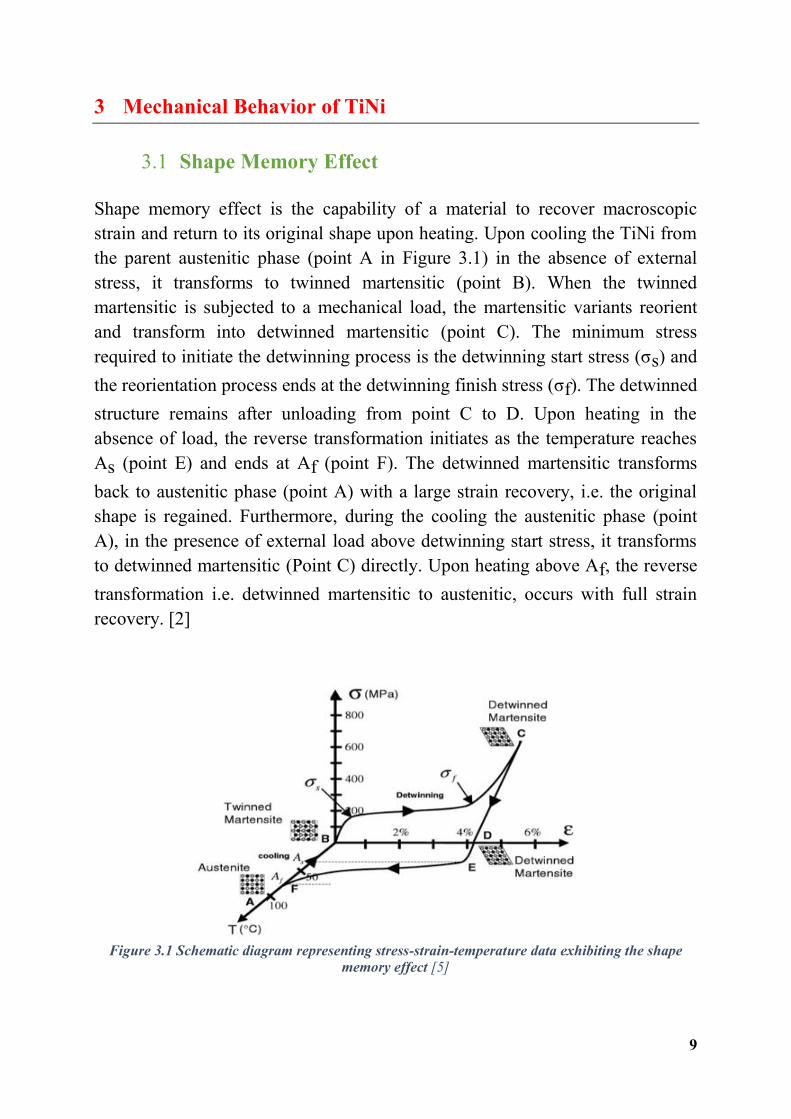
Shape memory effect is the capability of a material to recover macroscopic strain and return to its original shape upon heating. Upon cooling the TiNi from the parent austenitic phase (point A in Figure 3.1) in the absence of external stress, it transforms to twinned martensitic (point B). When the twinned martensitic is subjected to a mechanical load, the martensitic variants reorient and transform into detwinned martensitic (point C). The minimum stress required to initiate the detwinning process is the detwinning start stress (σs) and the reorientation process ends at the detwinning finish stress (σf). The detwinned structure remains after unloading from point C to D. Upon heating in the absence of load, the reverse transformation initiates as the temperature reaches As (point E) and ends at Af (point F). The detwinned martensitic transforms back to austenitic phase (point A) with a large strain recovery, i.e. the original shape is regained. Furthermore, during the cooling the austenitic phase (point A), in the presence of external load above detwinning start stress, it transforms to detwinned martensitic (Point C) directly. Upon heating above Af, the reverse transformation i.e. detwinned martensitic to austenitic, occurs with full strain recovery. [2]

Figure 3.1 Schematic diagram representing stress-strain-temperature data exhibiting the shape

memory effect [5]

10

3.2 Superelasticity Effect

The superelastic or pseudoelastic behavior is defined as the ability of a material to recover large strain upon unloading. The superelastic behavior of TiNi is associated with the stress induced martensitic transformation. During loading, the austenitic phase transforms to detwinned martensitic accompanied by large deformation. The reverse transformation from martensitic to austenitic occurs upon unloading, accompanied by large recoverable strain. The stress levels at

which the martensitic transformation starts and ends are named σMs

and σMf,

respectively. Similarly, the stress levels at which the reverse transformation

starts and ends are termed σAs

and σAf, respectively. Furthermore, upon

unloading full strain recovery occurs if the temperature is above Af and partial strain recovery occurs if the temperature is between Ms and Af. A schematic of a loading path demonstrating superelastic behavior of TiNi is shown in Figure 3.2.

3.3 Stress-Strain Curve of Superelastic TiNi Alloy A stress-strain curve for superelastic TiNi alloy is illustrated in Figure 3.2. The stress- strain curve represents a typical deformation behavior of superelastic alloys. The first initial rise in stress-strain curve of superelastic TiNi is due to elastic deformation of austenitic (A to B). This is followed by a stress plateau, a large recoverable deformation and phase transition from austenitic to martensitic as a result of stress-induced martensitic transformation (B to C). At the end of the plateau region, the material enters into an elastic/plastic deformation mode and behaves like conventional metals (C to D). Upon unloading, martensitic transforms back to the austenitic phase and the large deformation is recovered during the process. Upon unloading, martensitic to austenitic phase transition (D to A) occurs with large recoverable strain. The transformation from martensitic

to austenitic starts at σAs i.e. start stress for the reverse transformation and ends

at σAf i.e. finish stress for the reverse transformation. Materials exhibiting

superelastic behavior have large elongation during deformation due to suppression of necking and have high strain rate sensitivity (Dieter, 1976).

11

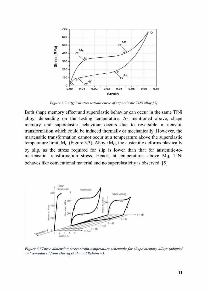
Figure 3.2 A typical stress-strain curve of superelastic TiNi alloy [5]

Both shape memory effect and superelastic behavior can occur in the same TiNi alloy, depending on the testing temperature. As mentioned above, shape memory and superelastic behaviour occurs due to reversible martensitic transformation which could be induced thermally or mechanically. However, the martensitic transformation cannot occur at a temperature above the superelastic temperature limit, Md (Figure 3.3). Above Md, the austenitic deforms plastically by slip, as the stress required for slip is lower than that for austenitic-to-martensitic transformation stress. Hence, at temperatures above Md, TiNi behaves like conventional material and no superelasticity is observed. [5]

Figure 3.3 ree e s o stress-stra -te erature sc e at c for s a e e ory alloys a a te

a re ro uce fro uer et al a y e

12

3.4 Hysteresis in NiTi The hysteresis is a function of composition in TiNi alloys and to the production process. During the heating and cooling cycle, changes in the lattice parameter are observed as the result of the martensitic transformation. But there is a difference between the temperature at which austenitic transforms to martensitic and martensitic to austenitic. The temperature difference between the forward transformation and the reverse transformation is known as hysteresis and depending on the material type, this temperature difference may vary between a few to hundreds of degrees Celsius. In general, SMA has a small hysteresis. The amount of martensitic formed is a function of the only temperature. [3]

Hysteresis grows with increasing stress for low Ni alloys (50,1%Ni). Hysteresis decrease with increasing stress for High Ni alloys (51,5%Ni)

The increase in hysteresis (in low nickel NiTi alloys) is linked to plastic relaxation of the internal stress in martensitic variants. The changes are attributed to the relaxation of elastic stored energy which is primarily due to dislocations emanating at martensitic/austenitic interfaces. Modifications in thermodynamics formulation are proposed to account for the change in hysteresis via a change in the elastic stored energy. [6]

4 Review of Literature about SMA

4.1 Electrical Resistivity-Based Study of Self-Sensing This study was conducted by 'Jian-Jun Zhang, Yue-hong Yin and Jian-Ying Zhu. They carried out a series of Thermal-electrical-mechanical experiments in other to verify the validity of the electrical resistivity model, whereby the SMA-AM (shape memory alloys artificial muscle) self-sensing function is well established under different stress condition. They reported that SMA can't be only used for actuating as an artificial hand muscle but also used as self-sensing. The self-sensing means that the SMA resistance can be used as the feedback signal for SMA length because the studies have proved that resistance plays an important role in SMA self-sensing. Therefore, the electrical resistivity variation of SMA is very complex to understand. Up to now, they are not too many models of self-sensing in the literature, Lan et al [7] ha e de eloped a self-sensing model based directl on the resistance to strain cur es using

pol nomial fitting without ta ing into consideration the electrical resisti it

13

effect ut o et al [8] in their studies proposed a micromechanical model of ER variations based on detailed analysis of the factors influencing ER variations from a microscopic perspective, such as stress, temperature, martensitic fraction, martensitic texture and R-phase distortion. They found out some reasonable agreement between the simulation and experimental result of electrical resistivity. Therefore they figure out that apart stress and temperature, the other factors mentioned above was really difficult to measure by real-time control method which is not conducive to feedback control application. [9]

4.1.1 Analysis of ER Properties of SMA Actuated AM

'Jian-Jun Zhang, Yue-hong Yin and Jian-Ying Zhu reported that the resistance-length (R-L) relationship must be well defined in order to have an accurate self-sensing even those the R-L relationship is still in the study to understand it very well; this is due to the complexity of electrical resistivity variations. As mentioned above, the graph shows the relationship between the ER and the different factors that influence it.

Figure 4.1 Relationship of influencing factors on ER variation of SMA wires.

4.1.2 Experimental Setup

In order to conduct their studies, they set up an experiment to determine the ER variations, during transformation, so they produce a series of thermal-electrical-mechanical experiments to the as-received SMA sample. The figure below

14

highlights the setup experiment. They use a sample with 0.15 mm of diameter and length of 117 mm and connected to different constant loads, that varying from 28 to 224 MPa and a helical bias spring with a stiffness of 390 N/m. The contraction force is then measured by using a load cell that connected to SMA, in order to measure the length, change of SMA the linear variable differential transformer (LVDT) with a resolution of 0.01 mm is used. The temperature is measured by using a thermocouple (Omega type K) positioned at the center of SMA. The SMA is heated by generating a current from an amplifier and the resistivity is calculated by the following formula. [9]

I is the heating current across the wire and U is the voltage, L is the length, Vo is the wire volume which in this case is considered constant. The experiment setup uses a computer equipped with a data acquisition card (NI USB-6211) to store and process the measurement.

Figure 4.2 Schematic diagram of the experimental setup.

4.1.3 Experimental Results

Figure 4.3 shows the experimental result of ER and Strain variations versus time of SMA. In red line is the ER and in blue line is the Strain. Upon heating, the ER response is non-monotonic with a sudden increase, decrease and increase

15

again, in segment BC the reverse transformation of SMA occurs, where they observe the decrease in ER because the ER of the martensitic is bigger than the ER of austenitic. in segment AB and CD, they are not any transformation, the increase of ER in mainly due to temperature increase, however, they observe a slight increase in strain in the segment AB and CD. Upon cooling, the opposite phenomenon of ER and strain occur and they observe that in segment EF, the ER increase because of the forward transformation meanwhile in segment DE and FG, the ER decrease is due to cooling. [9].

Figure 4.3 Experimental ER and strain response (a) and numerical temperature response

(b) of SMA wire during heating (I = 350 mA) and cooling (I = 50 mA).

4.1.4 Experimental Results at Various Constant Stresses

Figure 4.4 just highlights the experimental result of strain and ER curves during cooling and heating under a various constant applied stress. (A1..A2) denotes the start and (B1..B2) denote the end temperature of the reverse transformation (M to A). It is evident that the ER increase as the stress increase, compare to the reverse transformation, the forward transformation phase is slightly different, this is mainly due to the presence of the R-phase, the graph also shows that

16

whenever the R-phase appear, it becomes difficult to achieve a large deformation of SMA. For the example of the graph during the forward transformation phase (A-M), SMA achieves a transformation which yields to (5%) and the R-phase transformation achieves only a small change (less than 1%). [9].

Figure 4.4Experimental results of strain (a,b) and corresponding ER (c,d) changes of SMA

The graph below figures out the experimental and simulation result of resistivity versus strain of SMA. It is observed that upon M-A, the resistivity and strain have good linearity. The simulation behaves as the experimental one because of the linearity change in resistivity with stress. Therefore, upon A-M, a large error occurs between the simulation and the experimental results at lower applied stress mainly due to the appearance of R-phase during cooling. However, this

17

tends to decrease when the applied force increase and lead to the better linearity. [9].

Figure 4.5 Simulation and experimental results of ER vs. strain curves during M A (a) and A M (b) transformation at various constant stresses.

4.2 Feedback of Resistance

Many studies have been done in order to find a model that links the position of the SMA with one of its parameters easily measurable. Basically, this means that knowing the position of SMA, will be a benefit to use as a controller or sensor. One of these study state that using the SMA as sensor help to overcome the problem of weight and economical saving. But, unfortunately, the SMA manifest a strange behavior mainly due to it hysteresis characteristic. The study figures out an approximation linear relationship of the position with the electrical resistance of SMA. [10]

4.2.1 Open ring Test

Because of the sensibility of the electrical resistance to many factors as heat treatment, the composition of TiNi alloys and transformation process, a series of a test have been conducted in order to characterize the variation of electrical resistance with the position of SMA wire, in the first step the test was done in an open test ring in order to understand the deformation of SMA wire with it position under a constant load. The activation of the SMA wire, in this case, is done by applying an input voltage of a range 0,1 to 2,9 volt at a frequency of 1/6 Hz, in order to guarantee a complete transformation and avoid the destruction of SMA wire.

18

The tension applying to the SMA is reported in the graph below, and it is observed that both the current and the tension through the SMA wire are not sinusoidal, and this is due to the fact that the electrical varied between martensitic and austenitic. It is also reported the deformation of the SMA versus time and also in this case the graph is not sinusoidal. [10]

Figure 4.6 deformation of the actuator wire SMA with a sinusoidal tension input [10]

Figure 4.7 sinusoidal tension applied to the TiNi wire measured current. [10]

19

For this test, 15 activation cycles have been performed and it appears clear that with the hysteresis of the graph representing the position of the SMA with respect to the electrical current or the tension, it is not possible to use one of this parameter (current, tension) to derive the position of the SMA. The study also found out that the cycle is not repeatable because there are the caps between the cycle. [10]

Figure 4.8(a) Relationship between position and tension of the wire; (b) Relationship

between position and current of the wire [10]

Going on with this study, her is the relationship between electrical resistance and the deformation of SMA, the graph below shows the experiment that was performed. The SMA wire was still activated with an electrical input tension between 0,1-2,9 V, under two different load of 170 g and 500g respectively and frequency of 1/6 Hz for a corresponding time of 15 cycles. They observe also, in this case, the presence of the hysteresis. The hysteresis in the deformation and resistance curve is due to the difference of the phase transformation that occurs during the cooling where they pass from austenitic to R-phase and to martensitic and during heating where they pass directly from martensitic to austenitic. The study says that under some conditions during forwarding transformation the austenitic can transform to Martensitic through the R-phase because the R-phase has a crystallographic structure close to the one of martensitic but with a high resistance value. The decrease of the resistance at the end of the cooling process is the consequence of the transformation of R-phase to martensitic. The goal of the study was to derive the linear relationship between the resistance and the deformation of SMA. The experiment shows that increasing the load, the hysteresis in that relationship position tend to reduce as shown in the graphics below, this happens because under high mechanical loads the quantity

20

of austenitic that transforms to R-phase is reduced and more austenitic is transformed into martensitic. Based on this observation they increase the load applied to the SMA wire until the hysteresis disappears as is shown in the graph, then it appears easy to derive the relationship that was the goal of their study. [10]

Figure 4.9 (a) Relationship position-electrical resistance under constant load of 170 g; (b) Relationship position-electrical resistance under constant load of 500 g [10]

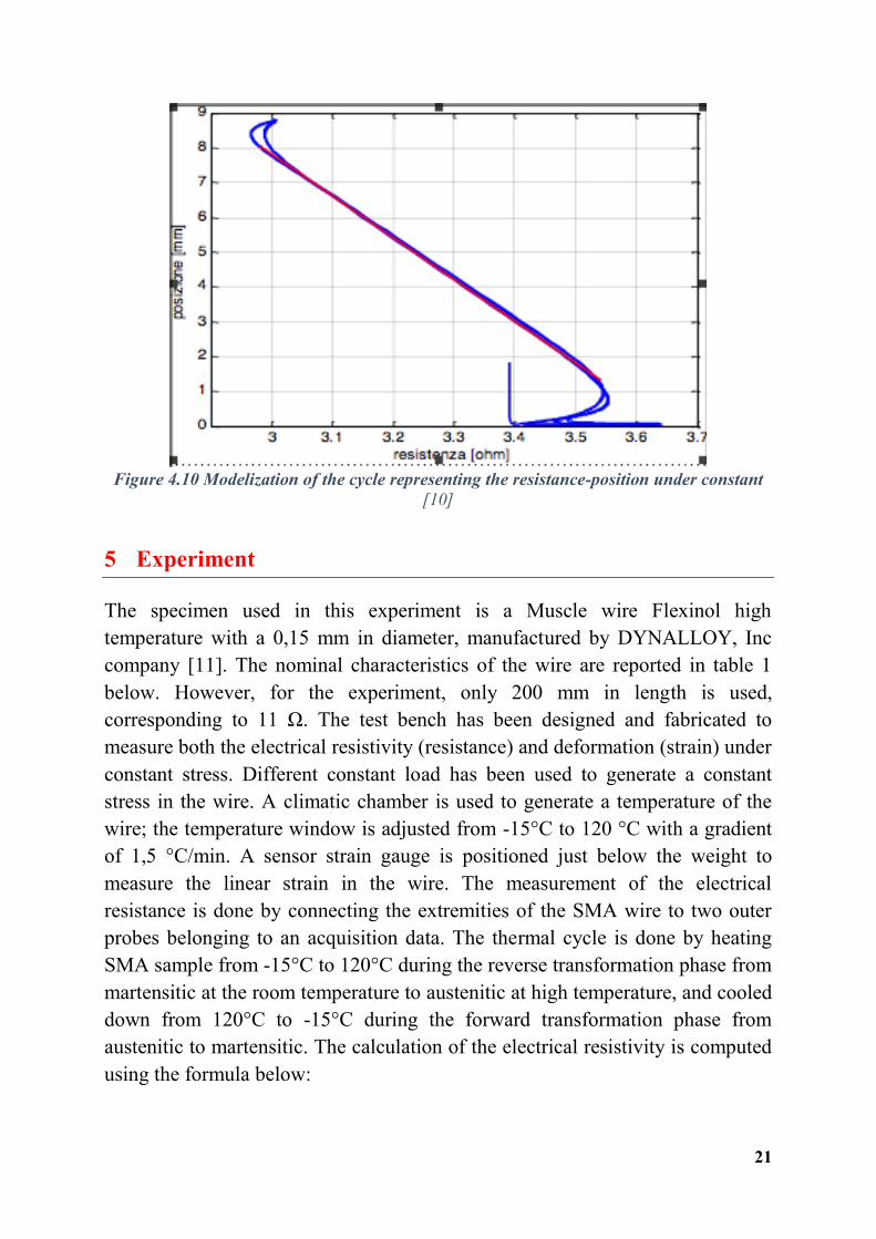
This result is obtained for the experiment that has been done in this topic pour the fifth cycle of the thermo-mechanical test under a constant load of 117 MPa. It is finally derived a linear relationship between the resistance and the position of SMA wire as it is represented in the figure 4.10, the linearity is well defined in almost all the range of the recovery strain, only the extremities appear to be strange and this will be taking into account during the realization of the feedback control. [10]

21

Figure 4.10 Modelization of the cycle representing the resistance-position under constant

[10]

5 Experiment The specimen used in this experiment is a Muscle wire Flexinol high temperature with a 0,15 mm in diameter, manufactured by DYNALLOY, Inc company [11]. The nominal characteristics of the wire are reported in table 1 below. However, for the experiment, only 200 mm in length is used, corresponding to 11 Ω. The test bench has been designed and fabricated to measure both the electrical resistivity (resistance) and deformation (strain) under constant stress. Different constant load has been used to generate a constant stress in the wire. A climatic chamber is used to generate a temperature of the wire; the temperature window is adjusted from -15°C to 120 °C with a gradient of 1,5 °C/min. A sensor strain gauge is positioned just below the weight to measure the linear strain in the wire. The measurement of the electrical resistance is done by connecting the extremities of the SMA wire to two outer probes belonging to an acquisition data. The thermal cycle is done by heating SMA sample from -15°C to 120°C during the reverse transformation phase from martensitic at the room temperature to austenitic at high temperature, and cooled down from 120°C to -15°C during the forward transformation phase from austenitic to martensitic. The calculation of the electrical resistivity is computed using the formula below:

22

Where R is the electrical resistance measured directly with Virtualbench of National instrument, L the length of the wire, and S is the cross-section of the wire used in the investigation.

Table 1 Nominal characteristic of SMA wire used for the experiment [11]

Figure 5.1 Test bench of the experiment. (1) Climatic chamber, (2)VirtualBench VB8012-307E2FE, (3) PC for Resistance acquisition, (4) NI USB 6211, (5) PC for resistance acquisition, (6) Sensor Laser, (7) weight, (8)-(9) Verticals supports, (10) additional conductor used to measure the resistance.

23

5.1 Description of the set-up

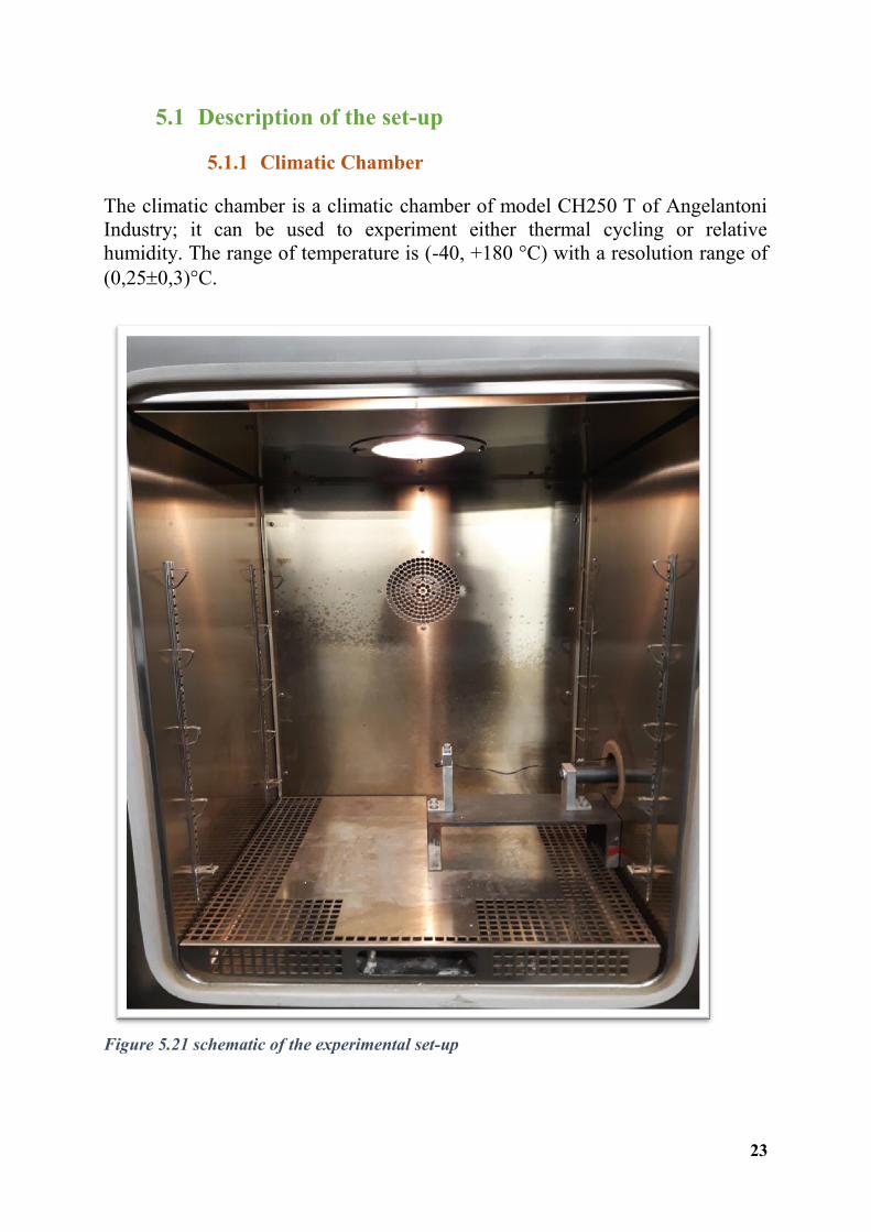
5.1.1 Climatic Chamber The climatic chamber is a climatic chamber of model CH250 T of Angelantoni Industry; it can be used to experiment either thermal cycling or relative humidity. The range of temperature is (-40, +180 °C) with a resolution range of (0,250,3)°C.

Figure 5.21 schematic of the experimental set-up

24

5.1.2 VirtualBench VB8012-307E2EF NI VirtualBench Combines an oscilloscope and other common instruments into a single device that connects to a PC or iPad. The VirtualBench All-in-One Instrument combines a mixed-signal oscilloscope with protocol analysis, an arbitrary waveform generator, a digital multimeter, a programmable DC power supply, and digital I/O. The all-in-one features are simple, convenient, and provide more efficient circuit design, debugging, and validation. The including software allows to view all measurements on a single screen and can be updated with free software releases to add functionality and value. The VirtualBench All-in-One Instrument easily integrates with LabVIEW software to provide programmatic control and automated test sequences. [12]

Figure 5.3 VirtualBench used to measure the resistance

5.1.3 NI USB 6211 data acquisition 16 AI (16-Bit, 250 kS/s), 2 AO (250 kS/s), 4 DI, 4 DO USB Multifunction I/O Device. The USB-6211 is a multifunction DAQ device. It offers analog I/O, digital input, digital output, and two 32-bit counters. The device provides an onboard amplifier designed for fast settling times at high scanning rates. It also features signal streaming technology that gives you DMA-like bidirectional high-speed streaming of data across USB. The device is ideal for test, control, and design applications including portable data logging, field monitoring, embedded OEM, in-vehicle data acquisition, and academic. The USB-6211 features a lightweight mechanical enclosure and is bus powered for easy portability. The included NI-DAQmx driver and configuration utility simplify configuration and measurements. [12]

25

Figure 5.4 NI USB 6211 for National Instruments

5.1.4 Supports The overall support is a metallic structure that was built in a previous work by a colleague in order to perform a similar work without measuring the resistance of SMA wire fig 5.5. The support assembly is formed with two verticals support (support-1 at the left and support-2 at the right), one horizontal support, and the basic support where the two vertical supports are fixed with the screws. The horizontal support is fixed to support-2 with a screw and out of the climatic chamber, it is fixed to a free rotating pulley fig 5.6. Three screws were used to fix the left end of SMA wire to support-1. [13]

Figure 5.5 support build to fix the SMA wire into the climatic chamber

26

Figure 5.6 System pulley and horizontal support

5.1.5 Computers

Two computers are used to store and display the data coming from the instruments of the data acquisition. To compute this task, into these computers some specific software and drivers are installed, for instance, the measurement of the temperature, the software WINKRATOS is installed, for the measurement of deformation (strain), SIGNALEXPRESS as software and NI‑DAQmx as the driver are needed. Finally, regarding the measurement of the resistance, LabVIEW is used as software and NI‑DAQmx as the driver.

5.1.6 Electrical connector The electrical connector is used in order to guarantee the correct fixation of SMA wire in the test bench, fig 5.7 below shows two of those connectors. The

27

most difficult part of the set-up was to find a trick to measure the resistance of SMA wire, in fact, the connection between the input of the VirtualBench and the two end of SMA wire where difficult to establish because SMA wire is into the climatic chamber. It is then necessary to find a trick to link them, so two addition conductors are used to solve the problem as it is highlighted in figure 5.7. Before doing this, the measurement of the two electrical conductors was first done to know how this could influence the result of the experiment, the measurement of additional conductors is performed under room temperature and the mean value obtained is 0 27 Ω, compared to the resistance of SMA wire at room temperature that is 11, it is like 40 times lower, and it is assumed that the value will be neglected.

Figure 5.7 electrical connector used to connect SAM wire with two additional conductors with negligible resistance.

28

5.1.7 Sensor laser Model optoNCDT 1300

OptoNCDT 1300 stands for high precision laser triangulation sensor, manufactured by Micro-epsilon company. The sensor laser is used to compute the recovery strain of the SMA wire as the deformation occurs. Therefore, it was set during the calibration of the sensor laser as it is shown in figure 5.9 a coefficient of 1,3. This simply means that 1 mA = 1,3 mm. This relashionship is very important because the coefficient of determination is close to one.

Figure 5.8 Sensor laser just below the weight

29

Figure 5.9 calibration of the Sensor laser [13]

5.1.8 Error made during the experimentation

As it was mentioned previously the metallic support was built by a colleague which was performing a similar experiment, but the difference is that the experiment did not include the measurement of the resistance. So one of the challenges was to find a good way to compute the measurement of the resistance of SMA wire, most review in the literature deal with joule effect and in that way it becomes quite easy to measure the resistance. But in this case, the increase and decrease of temperature were done by a climatic chamber. As it is shown in fig 5.9 below, they were a contact between SMA and the support, to avoid it, the use of an electrical connector was then necessary.

y = 0,7654x + 3,7245 R² = 0,99999

3

5

7

9

11

13

15

17

19

0 5 10 15 20

Co

rre

nte

[m

A]

Posizione slitta [mm]

salita 1

discesa 1

salita 2

discesa 2

salita 3

discesa 3

Lineare (discesa 3)

30

Figure 5.10 connection between the support and the wire using an electrical connector

6 Procedure of experimentation The procedure of the measurement involves two-step; The first step is to start the measurement and the second one is the end of the measurement and the acquisition of the data.

31

6.1 set-up and acquisition of the data of the measure

6.1.1 Temperature As mentioned in the previous paragraph of this report, the heating and cooling are done with a climatic chamber, and all the steps are controlled with a computer command panel through a software WINKRATOS, all the steps are developed in the following paragraph. To start the measurement of the temperature, first, run the program, open the control menu and click on Editor test program, then click on file to create a new program to control the temperature. Regarding the test that is performed in our case, the temperature range is from -15°C to 120°C for heating and from 120°C to -15°C for cooling. The cooling and heating are done through the segments, in this case, six segments, as it is highlighted in the table below, for each segment they provide the rank of the segment, how long take the segment (hour, min, second), the final set of the segment in °C, the gradient (°C/min) in case it is necessary, and finally depending on how they set is going to be controlled they check one or more of this item (control, max speed, waiting set, waiting time).

Figure 6.1 window of Editor program test with all the segments for heating and cooling.

32

The table below shows how all the segments have been done. Then the program is saved in the directory Chamber01\TestPrograms, it not really necessary to insert any extension but it is advised to put after the name of the file the extension (.prf), in our case the name of the file is AM Veloce. The file is a binary format so it can be edited only with the software WINKRATOS. To execute the program, under control menu click on Run/stop program test, select the file that was created before, for instance, AM Veloce and click OK, in the window they are: Starting segment, in this case, the starting segment is 1, the total number of repetition of the test, also in this case is 1, but in case someone wants to run the same test for more than on time, it is necessary to indicate the number of repetition, then press Ok to run the program. The program ends when all the segments and all the repetitions have been executed. However, the program could be arrested at any time by clicking on Run/stop program test and on Stop test. Now that the program is running the acquisition data can start, click on data acquisition in the menu, click on start new session, a new window open where it is possible to name a file, sampling interval (the lower the better is it, and better will be the resolution of the graph and the space occupied in the hard disk, 2 secs was used). The file can be selected, click on the button <selection file> give the name to the file where the data will be stored, the extension of the file is (.log) click ok to close the window and click again on the button < start acquisition data>. Now the program is running, it is possible to have an idea about each step of the program, clicking on the button control of the menu, again on < Monitoring program execution test>.

Figure 6.2 window that allows to start the record the data

33

Figure 6.3 Window panel to monitoring the measurement

segments 1 2 3 4 5 6

hour 0 0 1 0 1 0

minute 0 5 30 5 30 5

second 0 0 0 0 0 0

Final set °C -15 -15 120 120 -15 -15

Gradient °C/min 0 0 1.5 0 -1.5 0

control yes yes yes yes yes yes

Max speed yes no no no no no

Waiting set yes no yes yes yes yes

Waiting time no yes yes yes yes yes

Table 2 Table of different segment of the temperature measurement

34

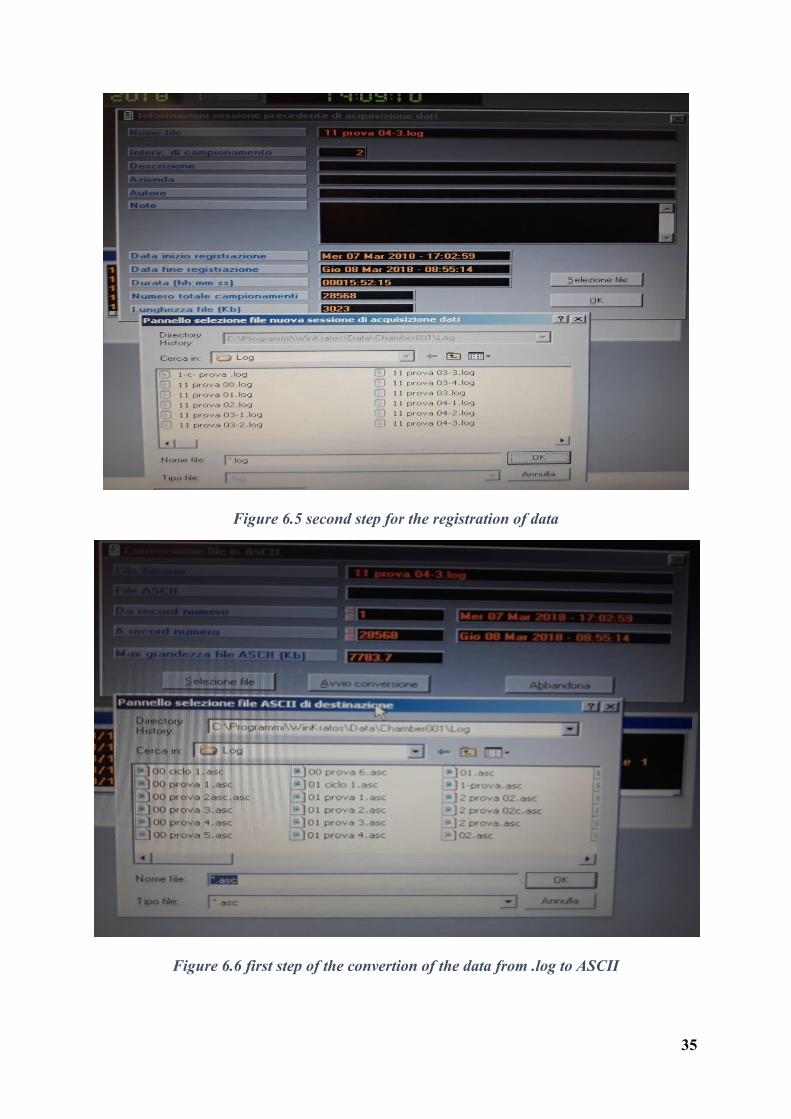
6.1.1.1 Conversion in file ASCII The file stored in the hard disk is in binary format, therefore, can be read only with WINKRATOS, in order to make it visible for any other application as Excel, Word it should be converted into ASCII file. Before the conversion into ASCII file, some step has to be done. Click on <Data acquisition> and on <Stop Actual session> to stop recording the data. Click on <acquisition data> in the menu bar, select <previous session>, <selection/information>, <selection file> to select the (.log) file to be converted, <OK> and the window will close, then click <acquisition data>, <previous session>, <conversion file in ASCII>, <selection file>, gives the name to the file ASCII and click <OK>, now click on <start conversion>, when the conversion ends click <cancel> and <leaves>. If all this step has been executed correctly, the file with extension (.log) is now converted into ASCII file.

Figure 6.4 window panel showing the first step to register the data

35

Figure 6.5 second step for the registration of data

Figure 6.6 first step of the convertion of the data from .log to ASCII

36

6.1.1.2 Conversion from ASCII file into Excel file Once the file is converted in ASCII file it can now be saved in Excel file, but once again the software <ZTreeWin> should be installed on the computer. Then open the ZTreeWin click on <Program>, scroll the file and click <WINKRASTOR>, <Data>, <Chmaber001>, double-click on <Log>, then choose the file name that was registered previously with extension (ASCII) and double-click, save the file on the desktop with Excel extension (.xls). The last step is to open the file save it again but, in <file name> remove the extension (.xls) and in <type of file> choose <Microsoft Excel(*.xls) and save it, now the file is ready to be open in Excel.

6.1.2 Deformation (Strain recovery) The acquisition and stored of the data of the temperature are done with National Instruments SignalExpress. Open NI SignalExpress, open a new project, a working space of SignalExpress is opened, on a menu bar click <Add Step>, <Acquire Signal>, <DAQmx Acquire>, <Analog Input>, and click on <Current> fig 6.7. At this step < Add Channels to Task> of USB-6211 is opened, choose the port (from ai0 to ai15) corresponding to the one that was used to build the electronic circuit connected to the Sensor Laser, in this case, it is (ai1) and click <OK>. Now <Step setup> menu is opened and has to be configured fig 6.8. In the menu: <configuration>, <Setting>, set the <Scaled units> to Amps and < Signal

Input Range> (Max=25m, Min=0m), <Sample to read> is 1, <Rate(Hz)> is 1.

<Advanced Timing>, < Sample Clock Type> is Internal, Timeout(s) is -1, fig 6.9.

In the menu bar <Connection Diagram> it is possible to display the construction diagram that was built in order to connect the Sensor Laser with the USB-6211, figure 6.10. Now that all thing has been set the program can be run, just click on <Run> in the menu bar and click on <Record> to start recording the test. Regarding the record of the data, once record button is operated, a window named <Logging Signals selection> appears as it is shown in the figure 6.11, it is then important to check Current under the <Signal to Include> otherwise the data will not be stored fig 6.11. Unfortunately, the program can't stop when the test is finished, so to stop the program just click on <Stop>. Data are now stored on the hard disk; the data can be visualized or exported. To visualize the graph, under <Logs> at bottom left click on the file corresponding to the format (date and hour) then, right click on <Current> once this small window is opened they data can be visualized or exported fig 2.12.

37

Figure 6.7 setting the measurement of the deformation, they is a relationship between current and deformation as it was mentioned before

Figure 6.8 virtual connection of USB 6211 that is connected to the sensor laser

38

Figure 6.9 configuration channel of virtual USB 6211

Figure 6.10 connection diagram that was built to connect USB 6211 to the sensor laser [13]

39

Figure 6.11check the box Current to record the data

Figure 6.12 Last step of the registration, here it is possible to visualize the graph and also to export to Excel

40

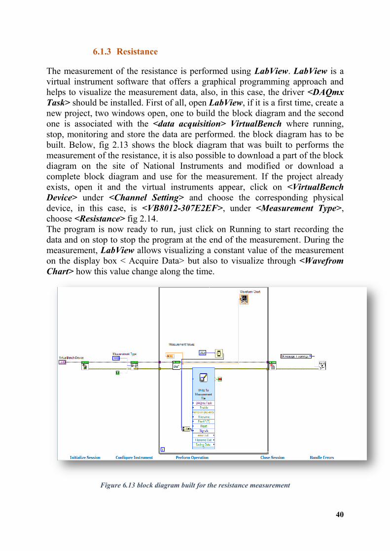
6.1.3 Resistance The measurement of the resistance is performed using LabView. LabView is a virtual instrument software that offers a graphical programming approach and helps to visualize the measurement data, also, in this case, the driver <DAQmx Task> should be installed. First of all, open LabView, if it is a first time, create a new project, two windows open, one to build the block diagram and the second one is associated with the <data acquisition> VirtualBench where running, stop, monitoring and store the data are performed. the block diagram has to be built. Below, fig 2.13 shows the block diagram that was built to performs the measurement of the resistance, it is also possible to download a part of the block diagram on the site of National Instruments and modified or download a complete block diagram and use for the measurement. If the project already exists, open it and the virtual instruments appear, click on <VirtualBench Device> under <Channel Setting> and choose the corresponding physical device, in this case, is <VB8012-307E2EF>, under <Measurement Type>, choose <Resistance> fig 2.14. The program is now ready to run, just click on Running to start recording the data and on stop to stop the program at the end of the measurement. During the measurement, LabView allows visualizing a constant value of the measurement on the display box < Acquire Data> but also to visualize through <Wavefrom Chart> how this value change along the time.

Figure 6.13 block diagram built for the resistance measurement

41

Figure 6.14 setting of the virtual instrument for the resistance measurement

7 Thermal Cycling Test

Fig 7.2, fig 7.3 and fig 7.4 show respectively resistivity-temperature, resistivity-recovery strain and the recovery strain-temperature, of the TiNi wire under constant stress during thermal cycling test. The graph clearly illustrates the transformation hysteresis, the variation of electrical resistivity is not due to the deformation but by the phase transformation, mainly because the resistivity is computed with the electrical resistance, the length, and the cross-section of the TiNi wire. In general, for common metal, the electrical resistivity increases linearly with the temperature increase without considering if the metal transforms or not, fig 7.1. Depending on the temperature the specimens could be full martensitic or full austenitic. Figure 7.3 highlights also the resistivity-deformation (recovery strain) curve of TiNi wire during thermal cycling test. A slight linearity of the hysteresis is

42

observed, it is reported in the literature that the electrical resistivity of SMA wire depends on the volume fraction of martensitic and austenitic phase. The graph provides the information about the different phase transformation, at room temperature, the SMA wire is a fully martensitic phase. Upon heating, the electrical resistivity remains almost constant with the increase in temperature until they reach austenitic start temperature, at the (Austenitic start temperature) the electrical resistivity starts to decrease. This decrease of electrical resistivity is due to the fact that the volume fraction of austenitic phase increase and the electrical resistivity of austenitic phase is lower than the ER of martensitic phase. The decrease of electrical resistivity is the consequence of the phase transformation of the martensitic to the austenitic phase. Therefore, when the (austenitic finish temperature) is reached the SMA is now 100% full austenitic phase, and the slight increase of the strain in that region is only due to the increase of the temperature. The opposite phenomenon is observed during the forward transformation (austenitic-martensitic) for instance cooling process. When the temperature starts to decrease, the electrical resistivity starts to increase linearly, and at (martensitic star temperaturet), they observe a drastic change of the electrical resistivity and a linear increase of the ER is not anymore observed, once at SMA wire is full martensitic means that all the austenitic have been transformed into martensitic. It is observed that the electrical resistivity of SMA varies with the volume fraction of each phase. It appears clear that it is not possible to derive a linear relationship between the resistivity and the temperature because this appears with a large hysteresis, contrary to the graph of the resistivity-recovery strain, it may be possible to derive this relationship. Figure 7.3 should not show hysteresis because the goal of this thesis is to derive the linear relationship between the two parameters but it is not the case, in fact, a slight hysteresis appears. Fig 7.3 shows the corresponding graph of the resistivity-recovery strain that has been performed. It is possible to see the relation between the graph of resistivity-temperature, and the graph of resistivity-recovery strain of SMA corresponding to , , , . The table 2 below resumes all the information of the graphs. The following paragraphs will illustrate the behaviors of the resistivity with the deformation during the thermo-mechanical cycle. The test performed is a thermo-mechanical cycle under constant stress, in the case of study, the loads are respectively 58,90MPa, 117Mpa and 176MPa, for each load five cycles are performed. 1

1 Ms(martensitic start temperature) Mf(martensitic finish temperature) As(austenitic start temperature) Af(austenitic finish temperature) SMA(Shape momery Alloys)

43

Figure 7.1 Resistivity versus temperature of common metal. [14]

Resistivity mm

0,017 0,01 0,01 0,02

Temperature °C 80,24 119,31 82,79 47,68

Recovery strain %

-0,2 -4,21 -4,45 -0,04

Table 3 Table that resumes the four important points of the transformation

The data present in table 3 above belong to the first cycle with a load of 176 MPa as it is shown in fig 7.2 and fig 7.3, it is used just to explain how to cycle work. These data in the change as the number of cycles increase.

44

Figure 7.2 First cycle of resistivity versus temperature under constant stress of 176 in red is heating and in blue is cooling

Figure 7.3 First cycle of resistivity versus deformation under constant stress of 176

80,24; 0,0171

119,31; 0,0100

82,79; 0,0094

0,0000

0,0050

0,0100

0,0150

0,0200

0,0250

-40 -20 0 20 40 60 80 100 120 140

Res

isti

vity

Ώm

m

Temperatura °C

176MPa--317g

As

Af Ms

Mf

[VALEUR X]

[VALEUR X]

[VALEUR X]

[VALEUR X]

0,0000

0,0050

0,0100

0,0150

0,0200

0,0250

-6 -5 -4 -3 -2 -1 0 1

Re

sist

ivit

y Ώ

mm

deformation %

176MPa--317g

45

Figure 7.4 First cycle recovery strain & temperature under constant stress of 176MPa

7.1 Result and Interpretation

7.1.1 Thermo-mechanical cycle under constant load of 58,90

MPa

Figure 7.5 resistivity-temperature of all the five cycle performed under constant load of 58,90 MPa

-5

-4

-3

-2

-1

0

-20 0 20 40 60 80 100 120D

efo

rmat

ion

%

Temperature °C recovery strain/ temperature

Heating Cooling

Fully Austenistic phase

Fully Martensitic phase

0

0,005

0,01

0,015

0,02

0,025

-40 -20 0 20 40 60 80 100 120 140

resi

stiv

ità

Ω m

m

temperature °C

Resistivity-temperature for five cycle at conatant stress 58,90MPa

cycle 1cycle 2cycle 3cycle 4cycle 5

46

Figure 7.6 resistivity-strain of all the five cycle performed under constant load of 58,90 MPa.

According to the information that the graph shows in figure 7.5, the hysteresis of the cycle diminishes as the number of cycle increase. This change is also accompanied by the change of the characteristics points of the curves, the gap between the first and the second cycle is very important during the forward transformation. Therefore, the first cycle could be considered as a thermo-mechanical calibration of SMA wire, in fact from the second cycle to the fifth cycle, the curves are quite close to each other. Upon heating, the austenitic start temperature (As) remains almost

constant when the number of cycles increases, but the electrical resistivity (ER) increase by moving up.

Regarding the austenitic finish temperature (Af), it is observed also a small shift to the right and an increase of the electrical resistivity.

During cooling, the martensitic start temperature (Ms) changes drastically mainly from the first cycle to the second and the electrical resistivity shift to the right with an increase after while it remains almost constant.

The same behavior is observed for the martensitic finish temperature (Mf), the only change is that the electrical resistivity shifts to the left and increase.

On the other hand, figure 7.6 provides information about the strain of all the five cycles, the same phenomenon of the graph in figure 7.5 is observed. The curves move as the number of cycle increase, the first one is the calibration of SMA and from the second to the fifth cycle is the test in question.

0

0,005

0,01

0,015

0,02

0,025

-6 -5 -4 -3 -2 -1 0 1

resi

stiv

ità

Ω m

m

Strain %

Resistivity-deformation for five cycle at conatant stress 58,90MPa

cycle 1cycle 2cycle 3cycle 4cycle 5

47

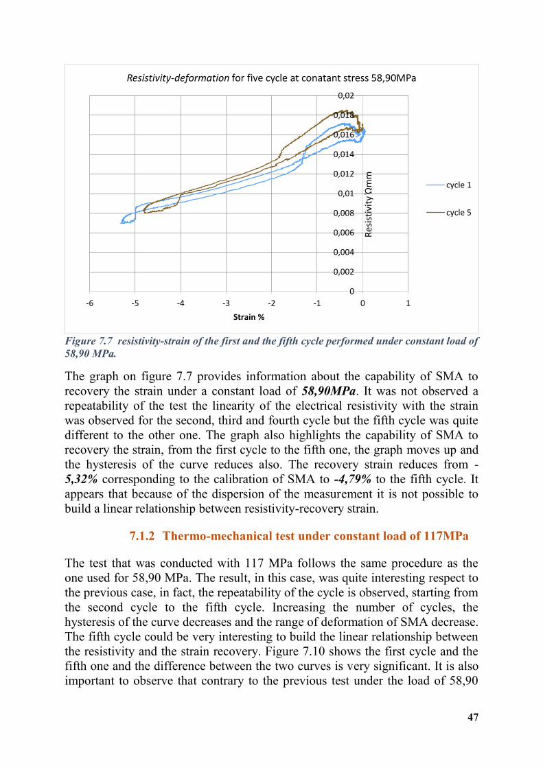
Figure 7.7 resistivity-strain of the first and the fifth cycle performed under constant load of 58,90 MPa.

The graph on figure 7.7 provides information about the capability of SMA to recovery the strain under a constant load of 58,90MPa. It was not observed a repeatability of the test the linearity of the electrical resistivity with the strain was observed for the second, third and fourth cycle but the fifth cycle was quite different to the other one. The graph also highlights the capability of SMA to recovery the strain, from the first cycle to the fifth one, the graph moves up and the hysteresis of the curve reduces also. The recovery strain reduces from -5,32% corresponding to the calibration of SMA to -4,79% to the fifth cycle. It appears that because of the dispersion of the measurement it is not possible to build a linear relationship between resistivity-recovery strain.

7.1.2 Thermo-mechanical test under constant load of 117MPa The test that was conducted with 117 MPa follows the same procedure as the one used for 58,90 MPa. The result, in this case, was quite interesting respect to the previous case, in fact, the repeatability of the cycle is observed, starting from the second cycle to the fifth cycle. Increasing the number of cycles, the hysteresis of the curve decreases and the range of deformation of SMA decrease. The fifth cycle could be very interesting to build the linear relationship between the resistivity and the strain recovery. Figure 7.10 shows the first cycle and the fifth one and the difference between the two curves is very significant. It is also important to observe that contrary to the previous test under the load of 58,90

0

0,002

0,004

0,006

0,008

0,01

0,012

0,014

0,016

0,018

0,02

-6 -5 -4 -3 -2 -1 0 1

Res

isti

vity

Ώm

m

Strain %

Resistivity-deformation for five cycle at conatant stress 58,90MPa

cycle 1

cycle 5

48

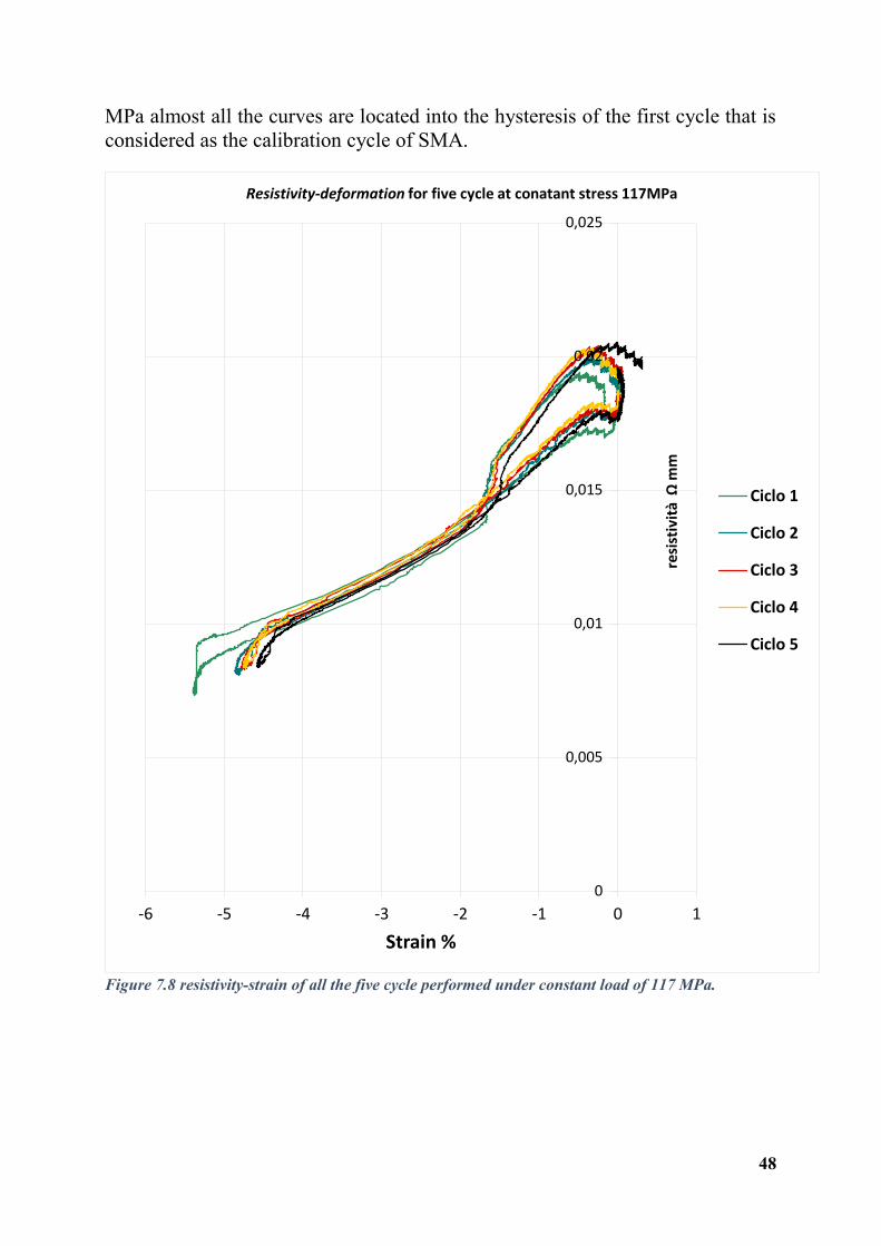
MPa almost all the curves are located into the hysteresis of the first cycle that is considered as the calibration cycle of SMA.

Figure 7.8 resistivity-strain of all the five cycle performed under constant load of 117 MPa.

0

0,005

0,01

0,015

0,02

0,025

-6 -5 -4 -3 -2 -1 0 1

resi

stiv

ità

Ω m

m

Strain %

Resistivity-deformation for five cycle at conatant stress 117MPa

Ciclo 1

Ciclo 2

Ciclo 3

Ciclo 4

Ciclo 5

49

Figure 7.9 resistivity-temperature of all the five cycle performed under constant load of 117 MPa.

Figure 7.10 resistivity-strain of the first and fifth cycle performed under constant load of 117 MPa.

0

0,005

0,01

0,015

0,02

0,025

-40 -20 0 20 40 60 80 100 120 140

resi

stiv

ità

Ω m

m

Temperatura °C

Resistivity-temperature for five cycle at conatant stress 117MPa

ciclo 1

ciclo 2

ciclo 3

ciclo 4

ciclo 5

0

0,005

0,01

0,015

0,02

0,025

-6 -5 -4 -3 -2 -1 0 1

resi

stiv

ità

Ω m

m

Strain %

Resistivity-deformation for five cycle at conatant stress 117MPa

Ciclo 1

Ciclo 5

50

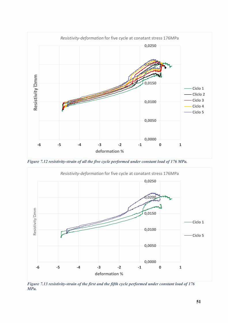
7.1.3 Thermo-mechanical test under constant load of 176 MPa The thermo-mechanical test conducted with the load of 176MPa almost close to the recovery Pull force of the SMA wire in the study. With this external stress, SMA behavior is very different to the two previous case. The calibration cycle is still big in hysteresis, but the increase of the number of cycles, move up and out of the hysteresis of the first cycle. However, some kind of repeatability is observed, the thickness of the hysteresis is almost constant, but the range of the strain recovery decreases and of course also the characteristics point of the cycle. As for the previous case, figure 7.13 shows the difference between the first and the fifth cycle. Under a constant load of 176 MPa it is evident that with the fifth cycles it is not possible to derive the linear relationship between the resistivity and the recovery strain.

Figure 7.11 resistivity-strain of all the five cycle performed under constant load of 176 MPa.

0,0000

0,0050

0,0100

0,0150

0,0200

0,0250

-40 -20 0 20 40 60 80 100 120 140

Res

isti

vity

Ώm

m

Temperature °C

Resistivity-deformation for five cycle at conatant stress 176MPa

Ciclo 1

Ciclo 2

Ciclo 3

Ciclo 4

Ciclo 5

51

Figure 7.12 resistivity-strain of all the five cycle performed under constant load of 176 MPa.

Figure 7.13 resistivity-strain of the first and the fifth cycle performed under constant load of 176 MPa.

0,0000

0,0050

0,0100

0,0150

0,0200

0,0250

-6 -5 -4 -3 -2 -1 0 1

Re

sist

ivit

y Ώ

mm

deformation %

Resistivity-deformation for five cycle at conatant stress 176MPa

Ciclo 1

Cliclo 2

Ciclo 3

Ciclo 4

Ciclo 5

0,0000

0,0050

0,0100

0,0150

0,0200

0,0250

-6 -5 -4 -3 -2 -1 0 1

Res

isti

vity

Ώm

m

deformation %

Resistivity-deformation for five cycle at conatant stress 176MPa

Ciclo 1

Ciclo 5

52

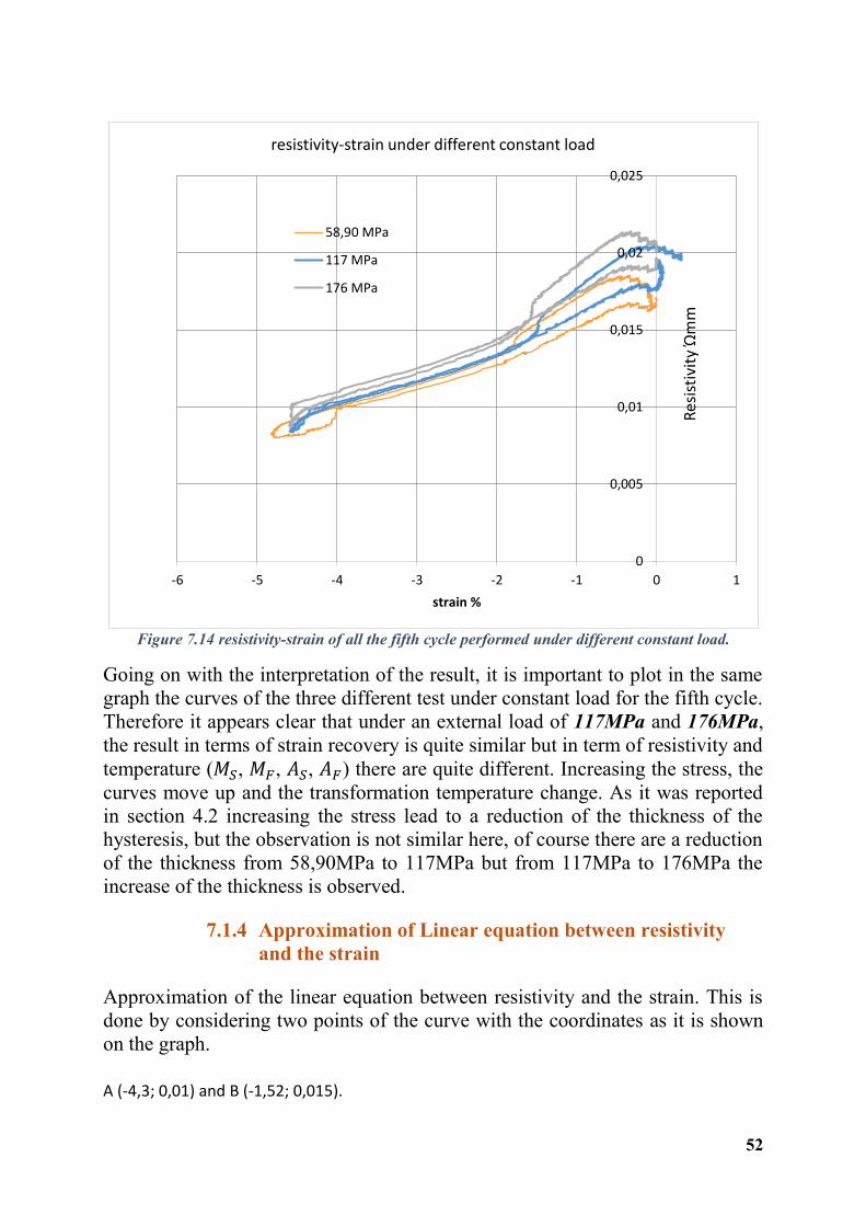
Figure 7.14 resistivity-strain of all the fifth cycle performed under different constant load.

Going on with the interpretation of the result, it is important to plot in the same graph the curves of the three different test under constant load for the fifth cycle. Therefore it appears clear that under an external load of 117MPa and 176MPa, the result in terms of strain recovery is quite similar but in term of resistivity and temperature ( , , , ) there are quite different. Increasing the stress, the curves move up and the transformation temperature change. As it was reported in section 4.2 increasing the stress lead to a reduction of the thickness of the hysteresis, but the observation is not similar here, of course there are a reduction of the thickness from 58,90MPa to 117MPa but from 117MPa to 176MPa the increase of the thickness is observed.

7.1.4 Approximation of Linear equation between resistivity

and the strain

Approximation of the linear equation between resistivity and the strain. This is done by considering two points of the curve with the coordinates as it is shown on the graph.

A (-4,3; 0,01) and B (-1,52; 0,015).

0

0,005

0,01

0,015

0,02

0,025

-6 -5 -4 -3 -2 -1 0 1

Res

isti

vity

Ώm

m

strain %

resistivity-strain under different constant load

58,90 MPa

117 MPa

176 MPa

53

The equation of the line is qmxy For the two points the equations are qmxy AA

qmxy BB

Solving the system of equation it follows that and

The approximation equation is

Figure 7.15 linear relationship between resistivity and the strain under constant stress of 117 MPa

Resistivity mm 0,018

0,011 0,011

0,02

Temperature °C 76,82 113,51 82,64 44,59

Recovery strain % -0,22 -4,07 -3,97 -0,32

Table 4 Transformation point of the cycle under constant load of 117MPa

-4,3; 0,01

-1,5; 0,015

0

0,005

0,01

0,015

0,02

0,025

-5 -4 -3 -2 -1 0 1

resi

stiv

ity Ωmm

strain %

resistivity-strain

54

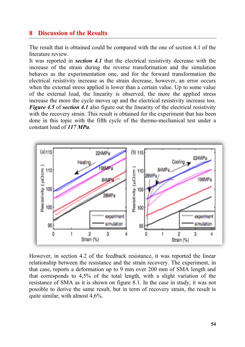
8 Discussion of the Results The result that is obtained could be compared with the one of section 4.1 of the literature review. It was reported in section 4.1 that the electrical resistivity decrease with the increase of the strain during the reverse transformation and the simulation behaves as the experimentation one, and for the forward transformation the electrical resistivity increase as the strain decrease, however, an error occurs when the external stress applied is lower than a certain value. Up to some value of the external load, the linearity is observed, the more the applied stress increase the more the cycle moves up and the electrical resistivity increase too. Figure 4.5 of section 4.1 also figure out the linearity of the electrical resistivity with the recovery strain. This result is obtained for the experiment that has been done in this topic with the fifth cycle of the thermo-mechanical test under a constant load of 117 MPa.

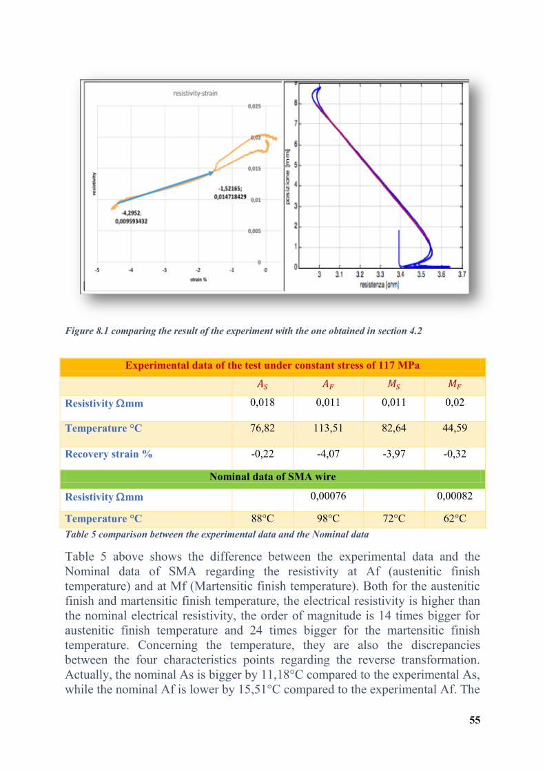
However, in section 4.2 of the feedback resistance, it was reported the linear relationship between the resistance and the strain recovery. The experiment, in that case, reports a deformation up to 9 mm over 200 mm of SMA length and that corresponds to 4,5% of the total length, with a slight variation of the resistance of SMA as it is shown on figure 8.1. In the case in study, it was not possible to derive the same result, but in term of recovery strain, the result is quite similar, with almost 4,6%.

55

Figure 8.1 comparing the result of the experiment with the one obtained in section 4.2

Experimental data of the test under constant stress of 117 MPa

Resistivity mm 0,018

0,011 0,011

0,02

Temperature °C 76,82 113,51 82,64 44,59

Recovery strain % -0,22 -4,07 -3,97 -0,32

Nominal data of SMA wire

Resistivity mm 0,00076 0,00082

Temperature °C 88°C 98°C 72°C 62°C Table 5 comparison between the experimental data and the Nominal data

Table 5 above shows the difference between the experimental data and the Nominal data of SMA regarding the resistivity at Af (austenitic finish temperature) and at Mf (Martensitic finish temperature). Both for the austenitic finish and martensitic finish temperature, the electrical resistivity is higher than the nominal electrical resistivity, the order of magnitude is 14 times bigger for austenitic finish temperature and 24 times bigger for the martensitic finish temperature. Concerning the temperature, they are also the discrepancies between the four characteristics points regarding the reverse transformation. Actually, the nominal As is bigger by 11,18°C compared to the experimental As, while the nominal Af is lower by 15,51°C compared to the experimental Af. The

56

same discrepancies appear also for the forward transformation, in fact, the nominal Ms is lower by 10,64°C compared to the experimental Ms meanwhile the nominal Mf is bigger by 17,41°C compared to the experimental Mf.

9 Conclusion

The goal of this work was to understand how SMA behaves during a thermo-mechanical cycle under different constant stress and also to find a linear relationship between the electrical resistivity and the recovery strain, the set-up of the experiment has been described, respect to some experiment that uses the effect joule to provide the temperature to SMA wire, a climatic chamber has been used to performs heating and cooling and the inertia of the climatic chamber should be considered. The analysis of the data shows that it is not evident to linearize the electrical resistance of the shape memory alloys with the recovery strain because of the slight variation of the electrical resistance, in fact regarding the formula that links all the parameters together,

if the

variation of the resistance is not very significant and considering that the section of SMA is almost constant, the linear relationship between resistivity and the recovery strain is just due to the variation in length of SMA. This deformation, in turn, is due to the variation of the volume fraction of martensitic and austenitic that occurs during the forward and the reverse transformation. Under all this consideration the linearization was done between the electrical resistivity and the strain, the value of the stress that allows to obtains the linearization is 117 MPa. Despite the fact that the linearization of the electrical resistivity with respect to the recovery strain was obtained, the experimental data did not match the nominal data in term of temperature transformation and in term of electrical resistivity. It was observed that as the stress and the number of cycle increase: The hysteresis of the curve is reduced. The range of recovery strain increase. The graph moves up. The characteristics temperature at which the transformation occurs

change. The electrical resistivity increase.

The future work on this topic could be: Using the same experimental set-up to understand why it was not possible to obtain the linearization between the electrical resistance and the recovery strain. It could also be interesting to

57

perform the same experiment with an increasing number of cycles may be up to 10 or 15. It will be quite interesting to compare this result with an effect joule experiment in other to see whether or not their results coincide.

58

10 Bibliography

[1] C. Lexcellent, Shape-memory Alloys Handbook, John Wiley & Sons, 2013. [2] R. Neupane, «Indentation and Wear Behavior of Superelastic TiNi Shape Memory

Alloy,» 2014. [3] R. R. Adharapurapu, «Phase transformations in nickel-rich nickel-titanium alloys :

influence of strain-rate, temperature, thermomechanical treatment and nickel composition on the shape memory and superelastic characteristics,» UC San Diego, 2007.

[4] A. S. Karthik Guda Vishnua, «Phase stability and transformations in NiTi from density functional theory calculations,» 2010 .

[5] P. K. K. a. D. C. Lagoudas, «Introduction to Shape Memory Alloys,» 2008. [6] R. H. H. Y. C. H. sehitoglu, "hysteresis in NiTi alloys," no. 115, 2004. [7] C. F. CC Lan, «Sensors and Actuators A: physica,» 2010. [8] V. Novak, P. Sittner, G. Dayananda, F. Braz-Fernandes et K. Mahesh, « Electric

resistance variation of NiTi shape memory alloy wires in thermomechanical tests: Experiments and simulation.,» Mater. Sci. Eng. A Struct., vol. 481, p. 127–133., 2008.

[9] Y.-H. Y. *. a. J.-Y. Z. Jian-Jun Zhang, «Electrical Resistivity-Based Study of Self-Sensing Properties for Shape Memory Alloy-Actuated Artificial Muscle,» 2013.

[10] P. Luigi, «Controllo in posizione di fili a memoria di forma,» 2005. [11] http://www.dynalloy.com/tech_data_wire.php. [12] http://www.ni.com/en-gb/shop/select/virtualbench-all-in-one-instrument. [13] A. Maurino, «charaterization Thermo-mechanical of SMA,» 2017. [14] https://www.tf.uni-kiel.de/matwis/amat/elmat_en/kap_2/illustr/g2_1_2.html.