Polynomials - the Australian Mathematical Sciences Institute

A guide for teachers – Years 11 and 121

2

3

4

5

6

7 8 9 10

11 12

Supporting Australian Mathematics Project

Functions: Module 10

Polynomials

Full bibliographic details are available from Education Services Australia.

Published by Education Services AustraliaPO Box 177Carlton South Vic 3053Australia

Tel: (03) 9207 9600Fax: (03) 9910 9800Email: [email protected]: www.esa.edu.au

© 2013 Education Services Australia Ltd, except where indicated otherwise. You may copy, distribute and adapt this material free of charge for non-commercial educational purposes, provided you retain all copyright notices and acknowledgements.

This publication is funded by the Australian Government Department of Education, Employment and Workplace Relations.

Supporting Australian Mathematics Project

Australian Mathematical Sciences InstituteBuilding 161The University of MelbourneVIC 3010Email: [email protected]: www.amsi.org.au

Editor: Dr Jane Pitkethly, La Trobe University

Illustrations and web design: Catherine Tan, Michael Shaw

Polynomials – A guide for teachers (Years 11–12)

Principal author: Dr Daniel Mathews, Monash University

Peter Brown, University of NSWDr Michael Evans AMSIAssociate Professor David Hunt, University of NSW

Assumed knowledge . . . . . . . . . . . . . . . . . . . . . . . . . . . . . . . . . . . . . 4

Motivation . . . . . . . . . . . . . . . . . . . . . . . . . . . . . . . . . . . . . . . . . . . 4

Content . . . . . . . . . . . . . . . . . . . . . . . . . . . . . . . . . . . . . . . . . . . . . 5

Some jargon . . . . . . . . . . . . . . . . . . . . . . . . . . . . . . . . . . . . . . . . . 5

Polynomial function gallery . . . . . . . . . . . . . . . . . . . . . . . . . . . . . . . . 6

Solving polynomial equations . . . . . . . . . . . . . . . . . . . . . . . . . . . . . . . 12

Behaviour of polynomials at infinity . . . . . . . . . . . . . . . . . . . . . . . . . . . 16

Stationary points . . . . . . . . . . . . . . . . . . . . . . . . . . . . . . . . . . . . . . 18

Sketching polynomial functions . . . . . . . . . . . . . . . . . . . . . . . . . . . . . 20

Polynomials from graphs . . . . . . . . . . . . . . . . . . . . . . . . . . . . . . . . . 24

Links forward . . . . . . . . . . . . . . . . . . . . . . . . . . . . . . . . . . . . . . . . . . 26

Approximating functions . . . . . . . . . . . . . . . . . . . . . . . . . . . . . . . . . . 26

Sums and products of roots . . . . . . . . . . . . . . . . . . . . . . . . . . . . . . . . 28

Solving cubics . . . . . . . . . . . . . . . . . . . . . . . . . . . . . . . . . . . . . . . . 30

Insolvability of quintics . . . . . . . . . . . . . . . . . . . . . . . . . . . . . . . . . . 31

Appendix . . . . . . . . . . . . . . . . . . . . . . . . . . . . . . . . . . . . . . . . . . . . 33

Lagrange interpolation formula . . . . . . . . . . . . . . . . . . . . . . . . . . . . . . 33

Rational root test . . . . . . . . . . . . . . . . . . . . . . . . . . . . . . . . . . . . . . 34

Fundamental theorem of algebra . . . . . . . . . . . . . . . . . . . . . . . . . . . . . 34

History . . . . . . . . . . . . . . . . . . . . . . . . . . . . . . . . . . . . . . . . . . . . . . 36

Évariste Galois . . . . . . . . . . . . . . . . . . . . . . . . . . . . . . . . . . . . . . . 36

Answers to exercises . . . . . . . . . . . . . . . . . . . . . . . . . . . . . . . . . . . . . 37

References . . . . . . . . . . . . . . . . . . . . . . . . . . . . . . . . . . . . . . . . . . . . 42

Polynomials

Assumed knowledge

• The content of the module Coordinate geometry.

• Familiarity with quadratic equations and functions and their graphs.

• The content of the module Functions II.

• The content of the module Introduction to differential calculus.

Motivation

Il y a quelque chose à compléter dans cette démonstration. Je n’ai pas le

temps . . . Après cela, il y aura, j’espère, des gens qui trouveront leur profit à

déchiffrer tout ce gâchis.

(There is something to complete in this proof. I do not have the time . . .

Later, there will be, I hope, some people who will find it to their advantage to

decipher all this mess.)

— Évariste Galois on polynomials, the night before his death, 29 May 1832.

By now we are familiar with linear and quadratic functions, i.e.,

f (x) = ax +b or f (x) = ax2 +bx + c,

where a,b,c are real constants. We know how to graph linear functions and how to solve

linear equations ax + b = 0. We also know how to draw graphs of quadratic functions

(which are parabolas) and how to solve quadratic equations ax2 +bx + c = 0.

It’s then natural to consider a slightly more complicated function, with just one more

term, an x3 term,

f (x) = ax3 +bx2 + cx +d .

Here a,b,c,d are real constants. The situation now becomes a bit more complicated. A

cubic function’s graph is not always of the same shape, and a cubic equation

ax3 +bx2 + cx +d = 0

A guide for teachers – Years 11 and 12 • {5}

is more difficult to solve than a quadratic one. In secondary school mathematics such

equations can only be solved in special cases. (We will give a sketch of a general method

in the Links forward section.)

But why stop at cubic functions? Why not add an x4 term? Why not an x3095283 term?

In general, if we allow any terms of the type axn , where a is a real constant and n a

non-negative integer, then the functions we obtain are called polynomial functions. A

general expression for a polynomial function is

f (x) = an xn +an−1xn−1 +an−2xn−2 +·· ·+a2x2 +a1x +a0.

The highest power n occurring is called the degree, and a0, a1, . . . , an are real numbers

called the coefficients.

Some examples of polynomials are the functions

f (x) = 3x3 − 11

3x +42, g (x) =p

7x3982 +5x13 −8 and h(x) = 6.

Polynomials are a natural type of function to consider: a generalisation of linear, quad-

ratic and cubic functions. They can sometimes be solved exactly. Their graphs can be

sketched. Many quantities in the real world are related by polynomial functions.

Importantly, any smooth function can be approximated by polynomials. So proficiency

in dealing with polynomials is also important.

The reader should be aware of the module Polynomials for Years 9–10, which provides

useful revision of some concepts in polynomials, and covers some interesting related

topics. This module is designed to complement the Years 9–10 module.

Content

Some jargon

We start by defining some words used to describe interesting bits and pieces of a polyno-

mial. Take a general polynomial function

f (x) = an xn +an−1xn−1 +·· ·+a1x +a0,

where an , an−1, . . . , a0 are real numbers with an 6= 0. We have already defined the degree n

and the coefficients a0, a1, . . . , an . The coefficient of xk is ak . The highest degree term

an xn is called the leading term and its coefficient an is called the leading coefficient.

If the leading coefficient is 1, the polynomial is called monic. The term a0 is called the

constant term.

{6} • Polynomials

Polynomials of degree 1, 2, 3, 4, 5 are respectively called linear, quadratic, cubic, quartic

and quintic. A degree-zero polynomial is just a constant function, such as f (x) = 3.

A root or a zero of a polynomial f (x) is a number r such that f (r ) = 0.

Example

Let f (x) = 18x4 −11x3 −7x +12. What is this polynomial’s degree, leading term, leading

coefficient, coefficient of x3, coefficient of x2, and constant term? Is f (x) monic?

Solution

The degree of f (x) is 4. The leading term is 18x4 and the leading coefficient is 18. The

coefficient of x3 is −11. The coefficient of x2 is 0. The constant term is 12. As the leading

coefficient is 18 (not 1), the polynomial f (x) is not monic.

A note of caution. Some of the coefficients may be zero. In the above example, the co-

efficient of x2 was zero; no x2 term is written. However the leading coefficient is always

non-zero, as it’s the coefficient of the highest power of x which actually appears.

Exercise 1

Show that 3 is a root of the polynomial 2x3 −8x2 +7x −3.

Polynomial function gallery

We can draw the graph of a polynomial function f (x) by plotting all points (x, y) in the

Cartesian plane with y-value given by f (x). In other words, we draw the graph of the

equation y = f (x).

We will examine some graphs of polynomial functions. We’ll start from simpler, low-

degree polynomials, making some observations as we go.

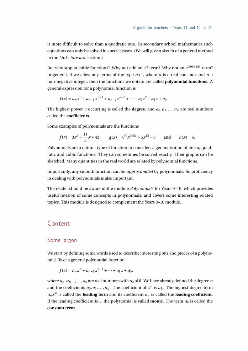
We are very familiar with graphing polynomials of degree 0 or 1, i.e., constant or linear

functions.

y

x0

3

y

x0

1

Graph of f(x) = 3. Graph of f(x) = 2x + 1.

12–


Quadratics

We should also be comfortable with graphing polynomials of degree 2, i.e., quadratic

functions. We know that we can always complete the square, so we can rewrite a quad-

ratic function f (x) = ax2 +bx + c as a(x −h)2 +k for some constants h and k. (Can you

find a formula for h and k in terms of a,b,c?) As we know from the module Functions II,

the graph of y = a(x −h)2 +k can be obtained from the standard parabola y = x2 by re-

flections, dilations and translations. In other words, any quadratic graph is a standard

parabola, suitably reflected, dilated and translated.

In particular, the turning point of y = a(x −h)2 +k is at (h,k).

Graph of f(x) = x2. Graph of f(x) = –2(x – 3)2 + 8.

y

x0

y

x0 1 5

–10

(3,8)

The sign of a (whether positive or negative) determines the general shape of the graph.

When a is positive, then as x → ±∞, we see that y → ∞, so the graph is curved like a

smile (‘happy’). If you imagine the graph as a road, and driving along it in the positive

x-direction, you would always be turning left. (In the language of calculus, the derivative

is increasing.) We say the graph is convex (or ‘concave up’).

On the other hand, when a is negative, then as x →±∞, we have y →−∞, so the graph is

curved like a frown (‘sad’). Driving along it in the positive x-direction, you would always

be turning right, and the graph is concave (or ‘concave down’).

Cubics

As we move from quadratic to cubic polynomials, things become more complicated. Un-

like the situation with quadratics, not every cubic graph is obtained from the standard

cubic graph y = x3 by reflections, dilations and translations. Indeed, if we consider three

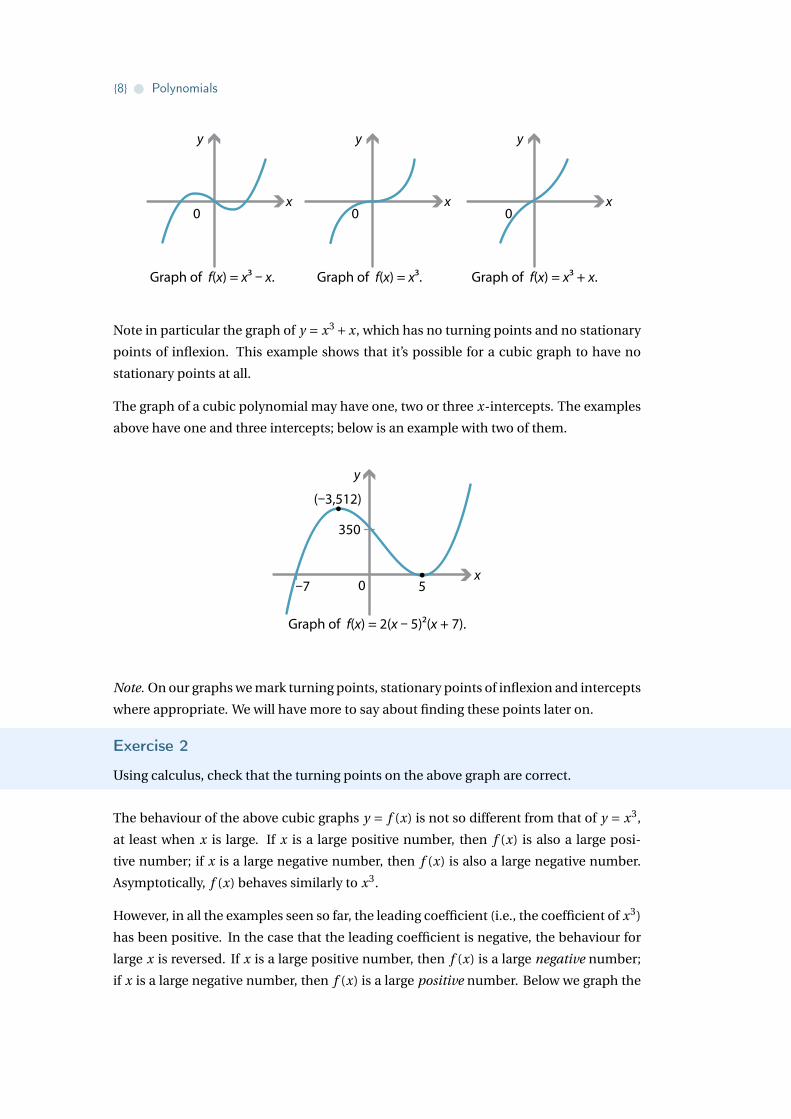
very simple cubic polynomials x3 −x, x3 and x3 +x, we get three distinct shapes.

{8} • Polynomials

Graph of f(x) = x3 – x. Graph of f(x) = x3 + x.Graph of f(x) = x3.

y

x0

y

x0

y

x0

Note in particular the graph of y = x3 +x, which has no turning points and no stationary

points of inflexion. This example shows that it’s possible for a cubic graph to have no

stationary points at all.

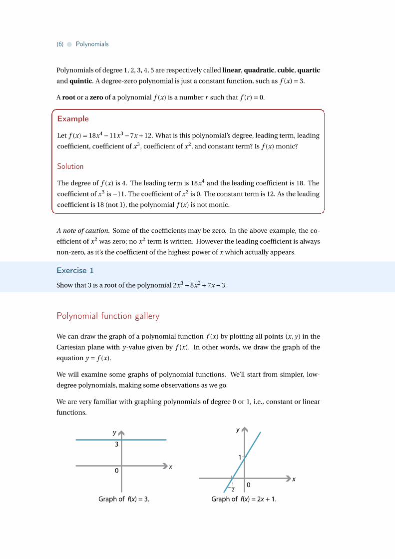
The graph of a cubic polynomial may have one, two or three x-intercepts. The examples

above have one and three intercepts; below is an example with two of them.

Graph of f(x) = 2(x – 5)2(x + 7).

y

x0 5–7

350

(–3,512)

Note. On our graphs we mark turning points, stationary points of inflexion and intercepts

where appropriate. We will have more to say about finding these points later on.

Exercise 2

Using calculus, check that the turning points on the above graph are correct.

The behaviour of the above cubic graphs y = f (x) is not so different from that of y = x3,

at least when x is large. If x is a large positive number, then f (x) is also a large posi-

tive number; if x is a large negative number, then f (x) is also a large negative number.

Asymptotically, f (x) behaves similarly to x3.

However, in all the examples seen so far, the leading coefficient (i.e., the coefficient of x3)

has been positive. In the case that the leading coefficient is negative, the behaviour for

large x is reversed. If x is a large positive number, then f (x) is a large negative number;

if x is a large negative number, then f (x) is a large positive number. Below we graph the


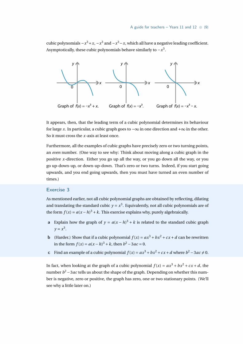
cubic polynomials −x3+x, −x3 and −x3−x, which all have a negative leading coefficient.

Asymptotically, these cubic polynomials behave similarly to −x3.

Graph of f(x) = –x3 + x. Graph of f(x) = –x3 – x.Graph of f(x) = –x3.

y

x0

y

x0

y

x0

It appears, then, that the leading term of a cubic polynomial determines its behaviour

for large x. In particular, a cubic graph goes to −∞ in one direction and +∞ in the other.

So it must cross the x-axis at least once.

Furthermore, all the examples of cubic graphs have precisely zero or two turning points,

an even number. (One way to see why: Think about moving along a cubic graph in the

positive x-direction. Either you go up all the way, or you go down all the way, or you

go up-down-up, or down-up-down. That’s zero or two turns. Indeed, if you start going

upwards, and you end going upwards, then you must have turned an even number of

times.)

Exercise 3

As mentioned earlier, not all cubic polynomial graphs are obtained by reflecting, dilating

and translating the standard cubic y = x3. Equivalently, not all cubic polynomials are of

the form f (x) = a(x −h)3 +k. This exercise explains why, purely algebraically.

a Explain how the graph of y = a(x −h)3 + k is related to the standard cubic graph

y = x3.

b (Harder.) Show that if a cubic polynomial f (x) = ax3 +bx2 + cx +d can be rewritten

in the form f (x) = a(x −h)3 +k, then b2 −3ac = 0.

c Find an example of a cubic polynomial f (x) = ax3 +bx2 +cx +d where b2 −3ac 6= 0.

In fact, when looking at the graph of a cubic polynomial f (x) = ax3 +bx2 + cx +d , the

number b2−3ac tells us about the shape of the graph. Depending on whether this num-

ber is negative, zero or positive, the graph has zero, one or two stationary points. (We’ll

see why a little later on.)

{10} • Polynomials

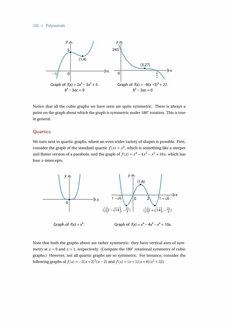
Graph of f(x) = 2x3 – 3x2 + 5. Graph of f(x) = –8(x –3)3 + 27.

y

x0

y

x0

(1,4)

5

–1

243

(3,27)

92

b2 – 3ac = 9 b2 – 3ac = 0

Notice that all the cubic graphs we have seen are quite symmetric. There is always a

point on the graph about which the graph is symmetric under 180◦ rotation. This is true

in general.

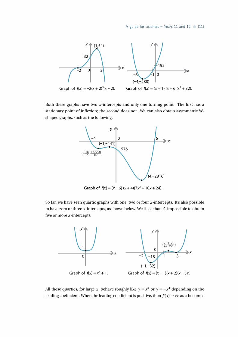
Quartics

We turn next to quartic graphs, where an even wider variety of shapes is possible. First,

consider the graph of the standard quartic f (x) = x4, which is something like a steeper

and flatter version of a parabola, and the graph of f (x) = x4 −4x3 − x2 +10x, which has

four x-intercepts.

y

x0

y

x0

(1,6)

Graph of f(x) = x4. Graph of f(x) = x4 – 4x3 – x2 + 10x.

21 – 6 1 + 6

( 2 + 14 , – )12

254( 2 – 14 , – )1

2254

Note that both the graphs above are rather symmetric: they have vertical axes of sym-

metry at x = 0 and x = 1, respectively. (Compare the 180◦ rotational symmetry of cubic

graphs.) However, not all quartic graphs are so symmetric. For instance, consider the

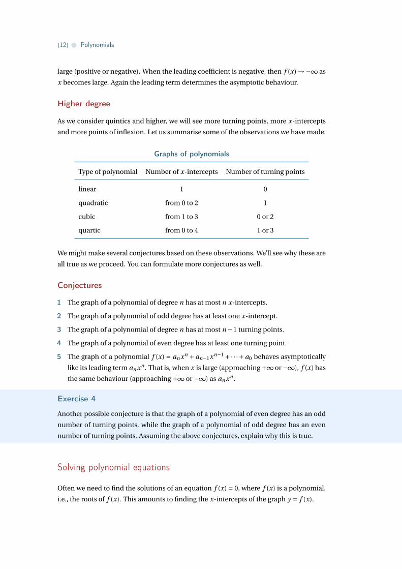
following graphs of f (x) =−2(x +2)3(x −2) and f (x) = (x +1)(x +6)(x2 +32).


y

x0

y

x0

192

Graph of f(x) = –2(x + 2)3(x – 2). Graph of f(x) = (x + 1) (x + 6)(x2 + 32).

2

32

–2

(1,54)

–1–6

(–4,–288)

Both these graphs have two x-intercepts and only one turning point. The first has a

stationary point of inflexion; the second does not. We can also obtain asymmetric W-

shaped graphs, such as the following.

y

x0

Graph of f(x) = (x – 6) (x + 4)(7x2 + 10x + 24).

6

–576

–4(–1,–441)

187

187200343(– , )

(4,–2816)

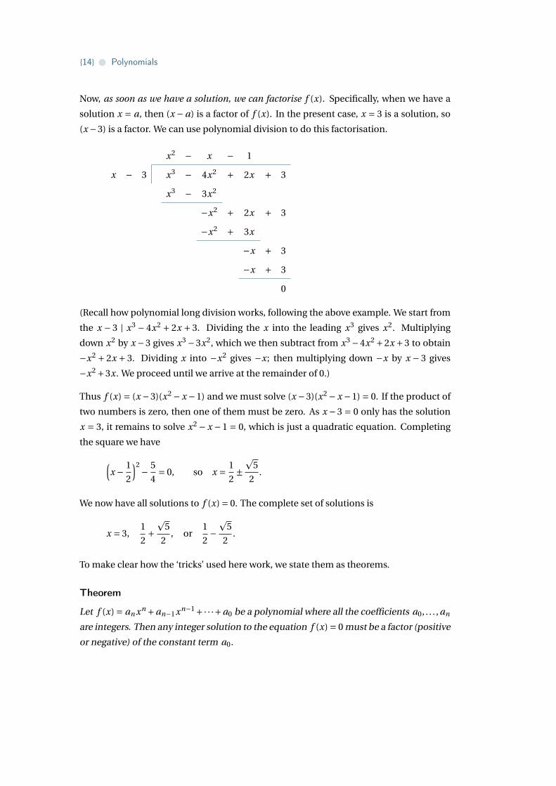
So far, we have seen quartic graphs with one, two or four x-intercepts. It’s also possible

to have zero or three x-intercepts, as shown below. We’ll see that it’s impossible to obtain

five or more x-intercepts.

y

x0

y

x0

(–1,–32)

Graph of f(x) = x4 + 1. Graph of f(x) = (x – 1)(x + 2)(x – 3)2.

31–2 –18

1125256( , )7

41

All these quartics, for large x, behave roughly like y = x4 or y = −x4 depending on the

leading coefficient. When the leading coefficient is positive, then f (x) →∞ as x becomes


large (positive or negative). When the leading coefficient is negative, then f (x) →−∞ as

x becomes large. Again the leading term determines the asymptotic behaviour.

Higher degree

As we consider quintics and higher, we will see more turning points, more x-intercepts

and more points of inflexion. Let us summarise some of the observations we have made.

Graphs of polynomials

Type of polynomial Number of x-intercepts Number of turning points

linear 1 0

quadratic from 0 to 2 1

cubic from 1 to 3 0 or 2

quartic from 0 to 4 1 or 3

We might make several conjectures based on these observations. We’ll see why these are

all true as we proceed. You can formulate more conjectures as well.

Conjectures

1 The graph of a polynomial of degree n has at most n x-intercepts.

2 The graph of a polynomial of odd degree has at least one x-intercept.

3 The graph of a polynomial of degree n has at most n −1 turning points.

4 The graph of a polynomial of even degree has at least one turning point.

5 The graph of a polynomial f (x) = an xn + an−1xn−1 +·· ·+ a0 behaves asymptotically

like its leading term an xn . That is, when x is large (approaching +∞ or −∞), f (x) has

the same behaviour (approaching +∞ or −∞) as an xn .

Exercise 4

Another possible conjecture is that the graph of a polynomial of even degree has an odd

number of turning points, while the graph of a polynomial of odd degree has an even

number of turning points. Assuming the above conjectures, explain why this is true.

Solving polynomial equations

Often we need to find the solutions of an equation f (x) = 0, where f (x) is a polynomial,

i.e., the roots of f (x). This amounts to finding the x-intercepts of the graph y = f (x).


When f is linear or quadratic, solving f (x) = 0 amounts to solving a linear or quadratic

equation. We know how to solve these.

For cubics and higher, the question is more difficult. There is a (complicated!) formula

for solving cubic equations, containing many +, −, ×, ÷ and radical signs (i.e.,p

, 3p

,4p

, etc.). There is also a (monstrously complicated!) formula for quartic equations. How-

ever, there is no such formula for a solution of a general quintic or higher degree equation.

This astonishing fact was proved by Niels Heinrik Abel in 1824, and independently by

the extraordinary French mathematician Évariste Galois quoted at the beginning of this

module. (For more on the brief, tumultuous and tragic life of Galois, see the History sec-

tion of this module.) Think about it: How would you go about proving that there is no

formula to solve an equation?

The insolvability of quintic polynomials is a university-level topic, although we shall say

something about it in the Links forward section. In secondary school mathematics, the

only higher degree polynomial equations encountered are ones with simple solutions.

One simple higher degree polynomial equation is x5 = 2, which obviously has solution

x = 5p

2. Another type of simple polynomial equation is found in the following exercise.

Exercise 5

Solve the equation x4 −5x2 +6 = 0.

For other simple polynomial equations, solutions can be found by educated trial and

error. Our next task is to learn the tricks for educated trial and error.

Solving by factorising

Let’s suppose we are asked to solve the cubic equation x3 − 4x2 + 2x + 3 = 0. So we let

f (x) = x3−4x2+2x +3, and we seek the roots of f (x). We begin finding solutions by trial

and error. Of course there are many guesses we could make!

The trick is to guess factors of the constant term. Here the constant term is 3, so we con-

sider factors of 3. We must be careful to check both the positive and negative factors of 3,

so we check 1, −1, 3, −3:

f (1) = 13 −4 ·12 +2 ·1+3 = 1−4+2+3 = 2,

f (−1) = (−1)3 −4(−1)2 +2(−1)+3 =−1−4−2+3 =−4,

f (3) = 33 −4 ·32 +2 ·3+3 = 27−36+6+3 = 0,

f (−3) = (−3)3 −4(−3)2 +2(−3)+3 =−27−36−6+3 =−66.

We have found a solution x = 3.


Now, as soon as we have a solution, we can factorise f (x). Specifically, when we have a

solution x = a, then (x −a) is a factor of f (x). In the present case, x = 3 is a solution, so

(x −3) is a factor. We can use polynomial division to do this factorisation.

x2 − x − 1

x − 3 x3 − 4x2 + 2x + 3

x3 − 3x2

−x2 + 2x + 3

−x2 + 3x

−x + 3

−x + 3

0

(Recall how polynomial long division works, following the above example. We start from

the x − 3 | x3 − 4x2 + 2x + 3. Dividing the x into the leading x3 gives x2. Multiplying

down x2 by x −3 gives x3 −3x2, which we then subtract from x3 −4x2 +2x +3 to obtain

−x2 + 2x + 3. Dividing x into −x2 gives −x; then multiplying down −x by x − 3 gives

−x2 +3x. We proceed until we arrive at the remainder of 0.)

Thus f (x) = (x −3)(x2 − x −1) and we must solve (x −3)(x2 − x −1) = 0. If the product of

two numbers is zero, then one of them must be zero. As x −3 = 0 only has the solution

x = 3, it remains to solve x2 − x −1 = 0, which is just a quadratic equation. Completing

the square we have

(x − 1

2

)2 − 5

4= 0, so x = 1

2±p

5

2.

We now have all solutions to f (x) = 0. The complete set of solutions is

x = 3,1

2+p

5

2, or

1

2−p

5

2.

To make clear how the ‘tricks’ used here work, we state them as theorems.

Theorem

Let f (x) = an xn +an−1xn−1+·· ·+a0 be a polynomial where all the coefficients a0, . . . , an

are integers. Then any integer solution to the equation f (x) = 0 must be a factor (positive

or negative) of the constant term a0.


ProofSuppose k is an integer solution, so f (k) = 0. Thus we have

ankn +an−1kn−1 +·· ·+a1k +a0 = 0,

and each ai is an integer. Now every term with a k in it is a multiple of k — that’s

every term on the left-hand side other than the constant term. But the terms on

the left-hand side have to add up to 0, so the final term a0 must be a multiple of k

as well. That is, k is a factor of a0.

Theorem (Factor theorem)

Let f (x) be a polynomial with real coefficients. If a is a real number such that f (a) = 0,

then (x −a) is a factor of f (x).

ProofWe can perform polynomial division, dividing f (x) by (x−a), to obtain a quotient

q(x) and a remainder r which is just a constant. (When you divide by a linear

polynomial, you get a constant remainder.) This means that

f (x) = (x −a)q(x)+ r.

Now substituting x = a into the above gives f (a) = 0+ r . As f (a) = 0, this means

the remainder r is 0. Thus f (x) = (x −a)q(x), and (x −a) is a factor of f (x).

Exercise 6

Solve the equation x3 +2x2 +3x +6 = 0.

Exercise 7

Prove the following corollary of the factor theorem: Let f (x) be a polynomial with real

coefficients. If r1,r2, . . . ,rk are distinct real numbers, each of which is a zero of f (x), then

the polynomial (x − r1)(x − r2) · · · (x − rk ) is a factor of f (x).

Number of solutions

We know that a linear equation ax +b = 0 always has one solution x =− ba . On the other

hand, a quadratic equation ax2 +bx + c = 0 may have zero, one or two real solutions.

For instance, the equation x2 +1 = 0 has no real solutions; while x2 −2x +1 = 0 has only

one real solution (‘repeated twice’) since it factorises to (x −1)2 = 0.


The quadratic formula tells us that the number of solutions of a quadratic equation

ax2 +bx + c = 0 is determined by the discriminant b2 −4ac. There are zero, one or two

solutions depending on whether b2 −4ac is negative, zero or positive.

For general polynomials, we can state the following.

Theorem

Let f (x) be a polynomial of degree n. Then f (x) = 0 has at most n distinct real solutions.

ProofSuppose instead that there were more than n distinct solutions. Let n +1 of these

distinct solutions be r1,r2, . . . ,rn+1. It follows from the factor theorem that the

polynomial (x − r1)(x − r2) · · · (x − rn+1) is a factor of f (x). (See Exercise 7.) Thus

f (x) = (x − r1)(x − r2) · · · (x − rn+1)q(x),

for some polynomial q(x). But now the right-hand side has degree at least n +1,

while f (x) has degree n. This is a contradiction, and so f (x) can have at most n

distinct solutions.

The above theorem is equivalent to saying that the graph y = f (x) of a polynomial f (x) of

degree n has at most n x-intercepts. So we have proved Conjecture 1 from the previous

section.

It turns out that if we allow square roots of negative numbers, leading to the complex

numbers, then we can always find n solutions (counting multiple roots) to an equation

of degree n. This is called the fundamental theorem of algebra. See the Appendix for

details.

Behaviour of polynomials at infinity

Understanding the behaviour of a polynomial function f (x) when x is large (that is, as

x →±∞) helps us to sketch the graph of y = f (x).

We’ve seen from examples that, for polynomial functions up to degree 4, the graph of

a polynomial f (x) = an xn + an−1xn−1 + ·· · + a0 behaves asymptotically like its leading

term an xn .

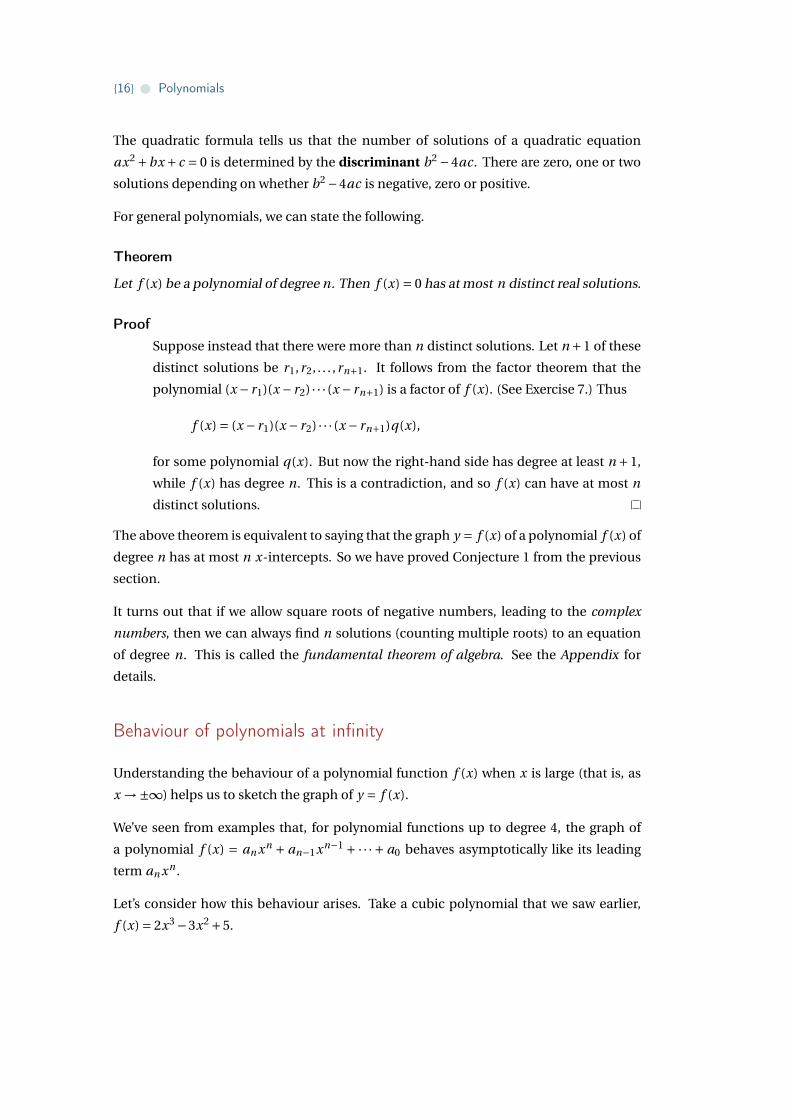
Let’s consider how this behaviour arises. Take a cubic polynomial that we saw earlier,

f (x) = 2x3 −3x2 +5.


Graph of f(x) = 2x3 – 3x2 + 5.

y

x0

(1,4)

–1

5

When x is large (positive or negative), x2 is much larger again, and x3 dwarfs them both.

So the x3 term will ‘dominate’ the others. One way to see this algebraically is to write

f (x) = 2x3 −3x2 +5 = 2x3(1− 3

2x+ 5

2x3

).

When x is large, both3

2xand

5

2x3 become very small, and so effectively the dominant

term is 2x3. This explains why, as seen on the graph,

f (x) →+∞ as x →+∞, and f (x) →−∞ as x →−∞.

A similar argument applies to any polynomial f (x) = an xn + an−1xn−1 + ·· · + a0: for

large x, the an xn term dominates the others.

Looking at the asymptotic behaviour, we can say that the graph y = xn is roughly U-

shaped when n is even, in the sense that xn → +∞ as x → ±∞. The actual graph may

have many turning points, but if we imagine ‘zooming out’ and looking only at the large-

scale picture when x is large, the graph is U-shaped. In a similar way, the graph of y = xn

is roughly /-shaped when n is odd. The behaviour of a polynomial graph y = f (x) when

x is large will depend on whether the degree of f (x) is even or odd, and on the sign of

the leading coefficient an . We can summarise the outcomes, along with rough shapes of

graphs when x is large, in a table.

Graph of a polynomial f (x) with leading term an xn

If n is and an is then as x →+∞ and as x →−∞ so shape is roughly

even positive f (x) →+∞ f (x) →+∞even negative f (x) →−∞ f (x) →−∞odd positive f (x) →+∞ f (x) →−∞odd negative f (x) →−∞ f (x) →+∞

This confirms our Conjecture 5.


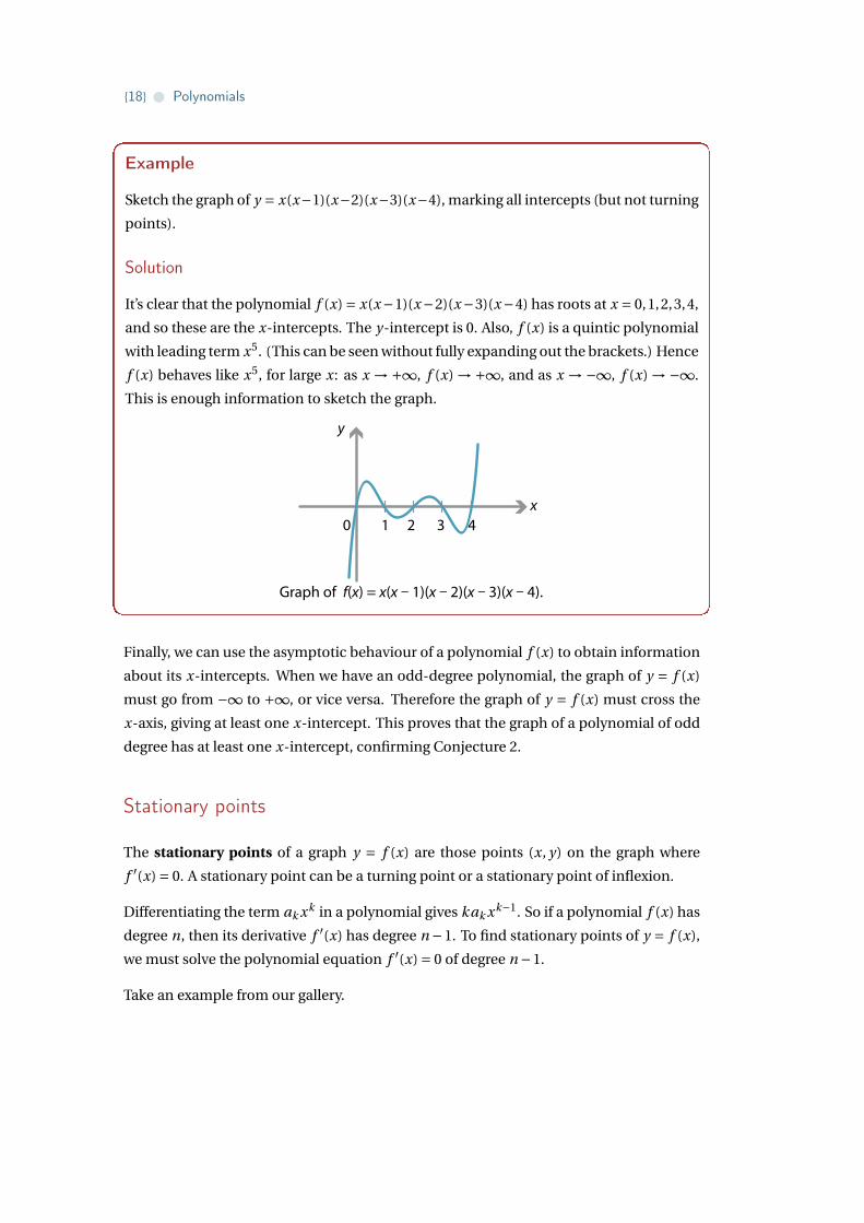
Example

Sketch the graph of y = x(x−1)(x−2)(x−3)(x−4), marking all intercepts (but not turning

points).

Solution

It’s clear that the polynomial f (x) = x(x−1)(x−2)(x−3)(x−4) has roots at x = 0,1,2,3,4,

and so these are the x-intercepts. The y-intercept is 0. Also, f (x) is a quintic polynomial

with leading term x5. (This can be seen without fully expanding out the brackets.) Hence

f (x) behaves like x5, for large x: as x →+∞, f (x) →+∞, and as x →−∞, f (x) →−∞.

This is enough information to sketch the graph.

Graph of f(x) = x(x – 1)(x – 2)(x – 3)(x – 4).

y

x0 1 2 3 4

Finally, we can use the asymptotic behaviour of a polynomial f (x) to obtain information

about its x-intercepts. When we have an odd-degree polynomial, the graph of y = f (x)

must go from −∞ to +∞, or vice versa. Therefore the graph of y = f (x) must cross the

x-axis, giving at least one x-intercept. This proves that the graph of a polynomial of odd

degree has at least one x-intercept, confirming Conjecture 2.

Stationary points

The stationary points of a graph y = f (x) are those points (x, y) on the graph where

f ′(x) = 0. A stationary point can be a turning point or a stationary point of inflexion.

Differentiating the term ak xk in a polynomial gives kak xk−1. So if a polynomial f (x) has

degree n, then its derivative f ′(x) has degree n −1. To find stationary points of y = f (x),

we must solve the polynomial equation f ′(x) = 0 of degree n −1.

Take an example from our gallery.


Example

Let f (x) = 2x3 −3x2 +5. Find the stationary points of the graph y = f (x).

Solution

We compute f ′(x) = 6x2−6x. To find stationary points we solve 6x2−6x = 0. Factorising

to 6x(x − 1) = 0 gives x = 0 or x = 1. Substituting these values of x gives f (0) = 5 and

f (1) = 4. So the stationary points are (0,5) and (1,4).

Note. Here f has degree 3, its derivative f ′ has degree 2, and so f ′(x) = 0 is a quadratic

equation.

The following exercise shows that a polynomial graph may have no stationary points. In

this exercise, the polynomial f again has degree 3 and its derivative f ′ has degree 2, but

the equation f ′(x) = 0 has no solutions.

Exercise 8

Let f (x) = x3 +x −2. Show that f (x) has no stationary points.

Next let’s consider the number of stationary points of a polynomial graph y = f (x), where

f (x) has degree n.

The stationary points are found by solving the equation f ′(x) = 0, which has degree n −1,

and hence has at most n−1 real solutions. Therefore the graph y = f (x) has at most n−1

stationary points. This confirms our Conjecture 3.

Slightly more trickily, if the degree n is even, then the degree n −1 of the derivative f ′(x)

is odd. So the graph of f ′(x) goes from −∞ to +∞, or vice versa. Therefore the graph of

f ′(x) crosses the x-axis somewhere, changing sign from positive to negative or from neg-

ative to positive. This gives a turning point of f (x). We have now confirmed Conjecture 4:

when n is even, the graph of f (x) has at least one turning point.

The next exercise gives a test for the number of stationary points of a cubic polynomial.

Exercise 9

Let f (x) = ax3 +bx2 + cx +d , where a,b,c,d are real numbers with a 6= 0. Show that:

a If b2 −3ac < 0, then y = f (x) has no stationary points.

b If b2 −3ac = 0, then y = f (x) has one stationary point.

c If b2 −3ac > 0, then y = f (x) has two distinct stationary points.


Sketching polynomial functions

Although polynomial graphs come in many shapes and sizes, they can be sketched once

we find a few of their features.

Example

Sketch the graph of y = f (x) where f (x) = 2x3 −6x2 −90x +350.

Solution

To find the x-intercepts, we solve f (x) = 2(x3−3x2−45x+175) = 0. Trying factors of 175

we find that x = 5 is a solution, so (x −5) is a factor. We can then completely factorise

f (x) as 2(x −5)2(x +7). So the x-intercepts are at x = 5,−7. To find the y-intercept, we

compute f (0) = 350.

To find the behaviour as x →±∞, note that f (x) behaves like the leading term 2x3. So

f (x) →+∞ as x →+∞, and f (x) →−∞ as x →−∞.

To find the stationary points, we solve f ′(x) = 0. Differentiating gives

f ′(x) = 6x2 −12x −90 = 6(x2 −2x −15).

Solving x2−2x−15 = 0 gives x =−3,5. Substituting these values into f gives f (−3) = 512

and f (5) = 0. So the stationary points are (−3,512) and (5,0).

From this information, we can sketch the graph of y = f (x).

y

x0–7 5

(–3,512)

350


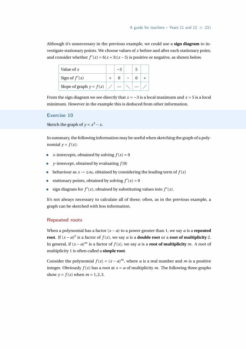
Although it’s unnecessary in the previous example, we could use a sign diagram to in-

vestigate stationary points. We choose values of x before and after each stationary point,

and consider whether f ′(x) = 6(x +3)(x −5) is positive or negative, as shown below.

Value of x −3 5

Sign of f ′(x) + 0 − 0 +Slope of graph y = f (x) � — � — �

From the sign diagram we see directly that x =−3 is a local maximum and x = 5 is a local

minimum. However in the example this is deduced from other information.

Exercise 10

Sketch the graph of y = x3 −x.

In summary, the following information may be useful when sketching the graph of a poly-

nomial y = f (x):

• x-intercepts, obtained by solving f (x) = 0

• y-intercept, obtained by evaluating f (0)

• behaviour as x →±∞, obtained by considering the leading term of f (x)

• stationary points, obtained by solving f ′(x) = 0

• sign diagram for f ′(x), obtained by substituting values into f ′(x).

It’s not always necessary to calculate all of these; often, as in the previous example, a

graph can be sketched with less information.

Repeated roots

When a polynomial has a factor (x −a) to a power greater than 1, we say a is a repeated

root. If (x − a)2 is a factor of f (x), we say a is a double root or a root of multiplicity 2.

In general, if (x − a)m is a factor of f (x), we say a is a root of multiplicity m. A root of

multiplicity 1 is often called a simple root.

Consider the polynomial f (x) = (x − a)m , where a is a real number and m is a positive

integer. Obviously f (x) has a root at x = a of multiplicity m. The following three graphs

show y = f (x) when m = 1,2,3.


y y

x x0 0a a

Graph of f(x) = x – a. Graph of f(x) = (x – a)2. Graph of f(x) = (x – a)3.

y

x0 a

An important fact to note is that the sign of f (x) changes at x = a when m is odd, and

does not change when m is even. (To see this, note that if x > a, then x − a is positive

and (x −a)m is also positive. If x < a, then x −a is negative; if m is even, then (x −a)m is

positive, while if m is odd, then (x −a)m is negative.)

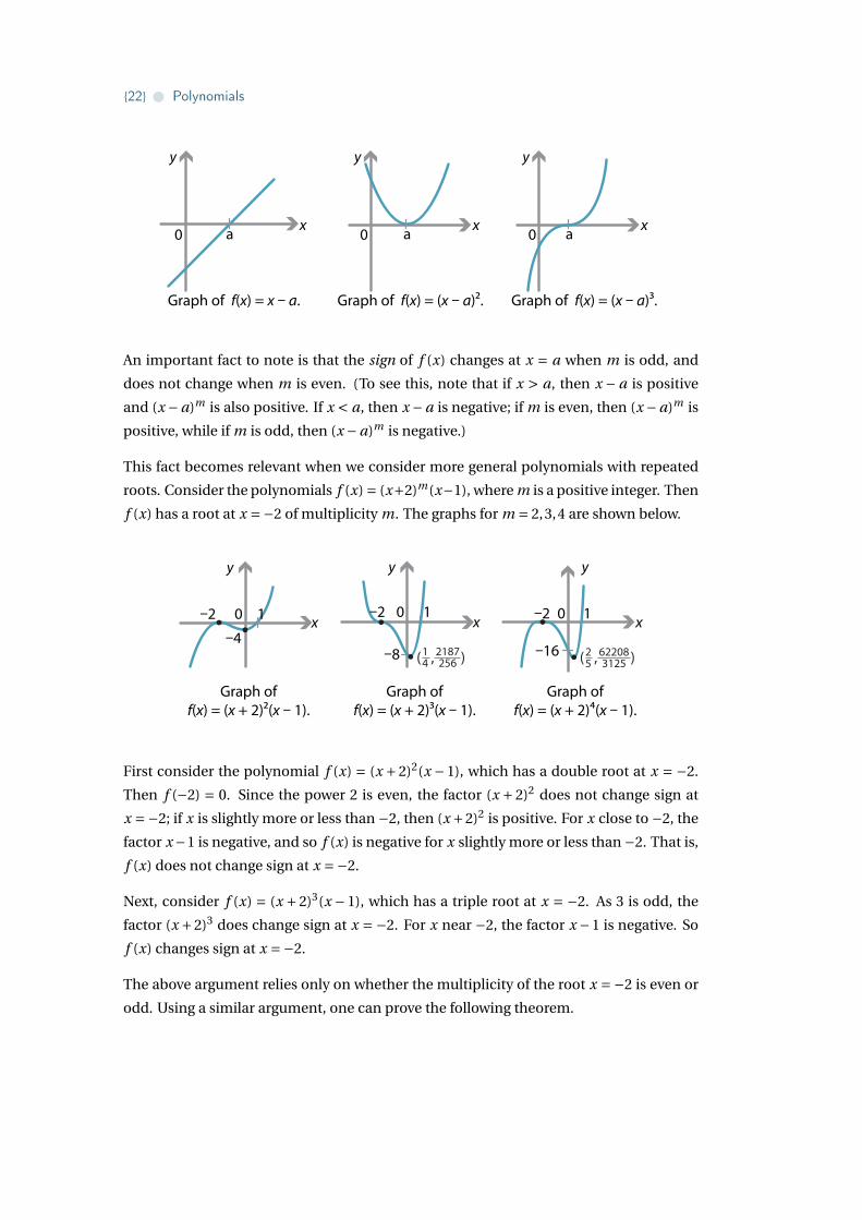
This fact becomes relevant when we consider more general polynomials with repeated

roots. Consider the polynomials f (x) = (x+2)m(x−1), where m is a positive integer. Then

f (x) has a root at x =−2 of multiplicity m. The graphs for m = 2,3,4 are shown below.

Graph of f(x) = (x + 2)2(x – 1).

Graph of f(x) = (x + 2)3(x – 1).

Graph of f(x) = (x + 2)4(x – 1).

y

x0

y

x0

y

x0 1 1–2

–4

–2 –2

–8

1

2187256( , )1

4–16 ( , )2

5622083125

First consider the polynomial f (x) = (x +2)2(x −1), which has a double root at x = −2.

Then f (−2) = 0. Since the power 2 is even, the factor (x + 2)2 does not change sign at

x =−2; if x is slightly more or less than −2, then (x +2)2 is positive. For x close to −2, the

factor x−1 is negative, and so f (x) is negative for x slightly more or less than −2. That is,

f (x) does not change sign at x =−2.

Next, consider f (x) = (x + 2)3(x − 1), which has a triple root at x = −2. As 3 is odd, the

factor (x +2)3 does change sign at x = −2. For x near −2, the factor x −1 is negative. So

f (x) changes sign at x =−2.

The above argument relies only on whether the multiplicity of the root x =−2 is even or

odd. Using a similar argument, one can prove the following theorem.


Theorem

Let f (x) be a polynomial with a root a of multiplicity m. Then f (x) changes sign at x = a

if and only if m is odd.

If a polynomial f (x) has a root at x = a of even multiplicity m, then f (x) does not change

sign at x = a, and yet f (a) = 0. Hence there must be a turning point and we obtain the

next theorem.

Theorem

Let f (x) be a polynomial with a root a of even multiplicity. Then the graph of y = f (x)

has a turning point at x = a.

Additionally, we note from the above graphs that a root of multiplicity 2 or more always

appears to be a stationary point. We can also prove this as a theorem.

Theorem

Let f (x) be a polynomial with a root a of multiplicity 2 or more. Then the graph of

y = f (x) has a stationary point at x = a.

ProofSince a has multiplicity at least 2, we know that (x −a)2 is a factor of f (x). (Maybe

higher powers of (x −a) divide into f (x), but (x −a)2 certainly does.)

We can then write f (x) = (x−a)2g (x) for some polynomial g (x). Differentiate f (x)

using the chain and product rules to obtain

f ′(x) = 2(x −a)g (x)+ (x −a)2g ′(x) = (x −a)[2g (x)+ (x −a)g ′(x)

].

Thus f ′(a) = 0 and so x = a is a stationary point.

Exercise 11

Sketch the graph of y = x4 −x2.

Transformation methods

We’ve seen from the module Functions II that, if we take the graph of y = f (x) and dilate

or translate it in the x and y directions, or reflect in the axes, then the result is a graph of

y = a f (b(x − c))+d , for some real numbers a,b,c,d .


We can sometimes use this idea in reverse, as in the following example. It’s easier than

using the standard method.

Example

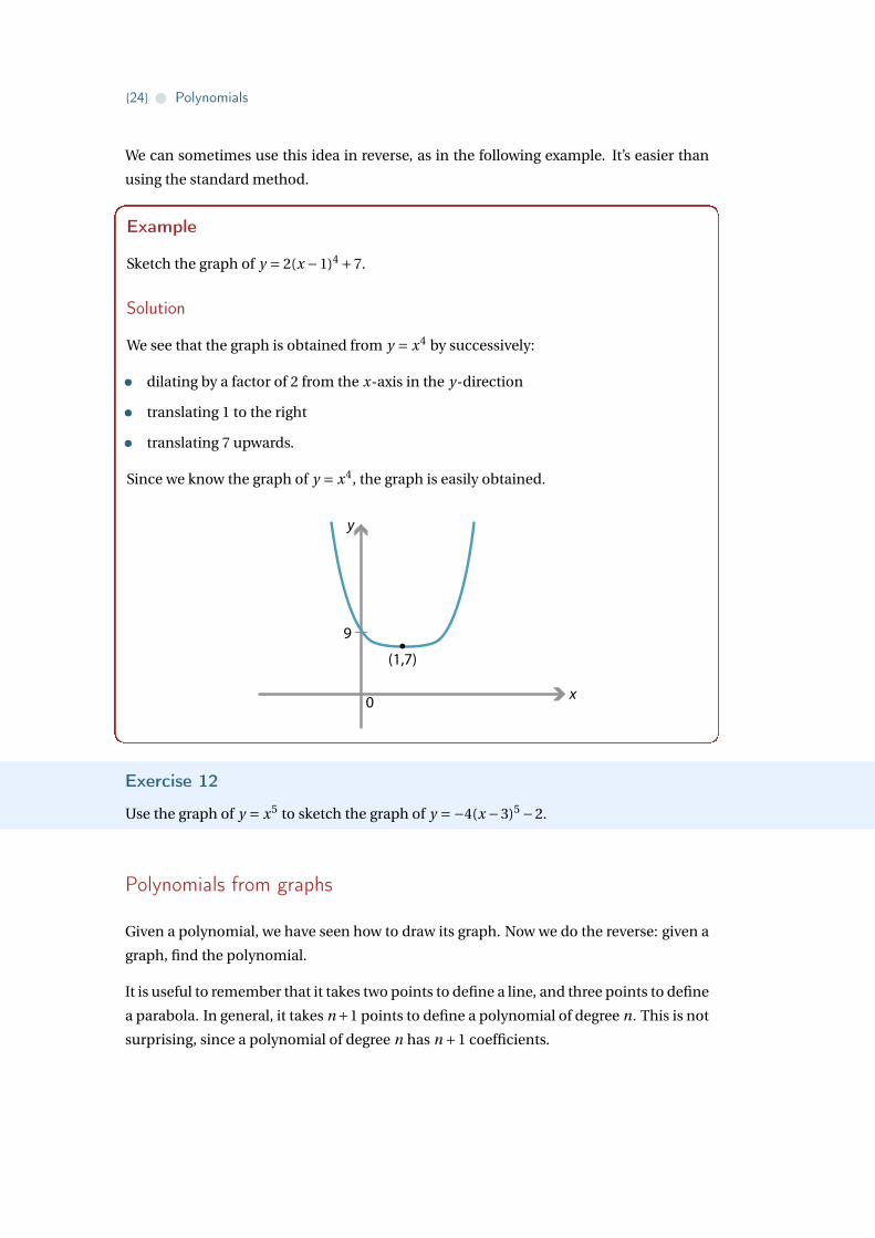
Sketch the graph of y = 2(x −1)4 +7.

Solution

We see that the graph is obtained from y = x4 by successively:

• dilating by a factor of 2 from the x-axis in the y-direction

• translating 1 to the right

• translating 7 upwards.

Since we know the graph of y = x4, the graph is easily obtained.

y

0 x

(1,7)

9

Exercise 12

Use the graph of y = x5 to sketch the graph of y =−4(x −3)5 −2.

Polynomials from graphs

Given a polynomial, we have seen how to draw its graph. Now we do the reverse: given a

graph, find the polynomial.

It is useful to remember that it takes two points to define a line, and three points to define

a parabola. In general, it takes n+1 points to define a polynomial of degree n. This is not

surprising, since a polynomial of degree n has n +1 coefficients.


Example

The graph y = f (x) of the quartic polynomial f (x) is drawn below. Find f (x).

y

0x

(–3,108)

3–2–6

(Reality check: Five points are specified in the graph, namely four x-intercepts and one

extra point. This is the right number of points to determine a quartic polynomial.)

Solution

The graph shows four x-intercepts at x =−6,−2,0,3. Hence (x +6), (x +2), x and (x −3)

are all factors of f (x). Multiplying these factors together already gives a quartic; the

only other possible factor is just a constant. So f (x) = c(x + 6)(x + 2)x(x − 3) for some

constant c. Since f (−3) = 108, we have 108 = c ·3 · (−1) · (−3) · (−6), so 108 = −54c and

c =−2. Thus f (x) =−2(x +6)(x +2)x(x −3).

The above example demonstrates that knowing the roots is not enough information to

determine a polynomial. Indeed, in the example, there is a whole family of polynomials

f (x) = c(x +6)(x +2)x(x −3) with the same roots, where c is any (non-zero) real number.

We needed the extra data of a point on the curve to determine c.

In general:

• An x-intercept at x = a implies that (x −a) is a factor of f (x).

• A y-intercept at y = c implies that f (0) = c, i.e., the constant term in f (x) is c.

• A given point (p, q) on the graph implies that f (p) = q .

If we are just given points on the graph of y = f (x), one way to find the polynomial is by

simultaneous equations, as the following example shows.


Example

Find the quadratic polynomial f (x) whose graph passes through the three points (1,−2),

(2,−1) and (3,2).

Solution

Let the polynomial be f (x) = ax2 +bx + c. We are given that f (1) = −2, f (2) = −1 and

f (3) = 2, so we have the simultaneous equations

a +b + c =−2 (1)

4a +2b + c =−1 (2)

9a +3b + c = 2. (3)

Subtracting (2)− (1) and (3)− (2) gives 3a +b = 1 and 5a +b = 3. Subtracting these two

equations gives 2a = 2, so a = 1. Substituting a = 1 back into these equations gives

b =−2 and then c =−1. So f (x) = x2 −2x −1.

In principle we could use the above method to find, say, a quintic through six given

points, or a degree-100 polynomial through 101 given points; it just becomes increas-

ingly tedious to eliminate the variables and solve the simultaneous equations!

As it turns out (and beyond the secondary school curriculum), there is actually a for-

mula for the polynomial through a given set of points, called the Lagrange interpolation

formula, discussed in the Appendix.

Links forward

Approximating functions

If we are given a function f (x), we can try to find a polynomial p(x) which approximates

that function. Indeed, if we know some of the values of f ,

f (x1) = y1, f (x2) = y2, . . . , f (xn) = yn ,

then we can find a polynomial p(x) which takes those values, as we just saw.

That is one type of approximation. The following example shows another type of approx-

imation: finding a polynomial which agrees with f , and its derivatives, at a point.


Example

Find a quadratic polynomial p(x) which approximates the function f (x) = cos x in the

sense that p agrees with f in value, and in its first two derivatives, at x = 0, i.e.,

p(0) = f (0), p ′(0) = f ′(0) and p ′′(0) = f ′′(0).

(Reality check: We’re asked to find a quadratic polynomial satisfying three conditions.

This makes sense since a quadratic has three coefficients.)

Solution

First of all we can compute f ′(x) =−sin x and f ′′(x) =−cos x, so f (0) = 1, f ′(0) = 0 and

f ′′(0) =−1. Thus we want to find a quadratic polynomial p(x) such that

p(0) = 1, p ′(0) = 0 and p ′′(0) =−1.

Let p(x) = ax2 +bx + c, where a,b,c are real coefficients. Then we have p ′(x) = 2ax +b

and p ′′(x) = 2a, so the three equations above become

c = 1, b = 0 and 2a =−1.

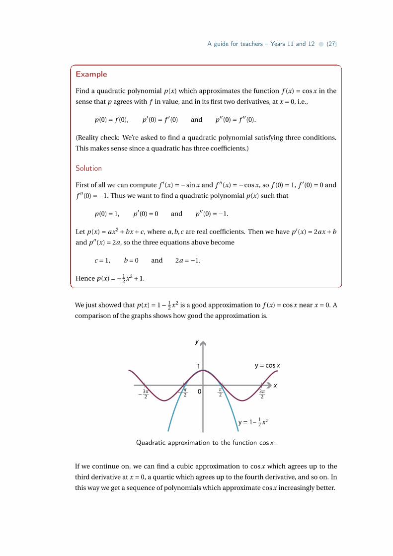
Hence p(x) =−12 x2 +1.

We just showed that p(x) = 1− 12 x2 is a good approximation to f (x) = cos x near x = 0. A

comparison of the graphs shows how good the approximation is.

y

0x

y = cos x1

32– 3

22

y = 1 – x212

2–

Quadratic approximation to the function cos x .

If we continue on, we can find a cubic approximation to cos x which agrees up to the

third derivative at x = 0, a quartic which agrees up to the fourth derivative, and so on. In

this way we get a sequence of polynomials which approximate cos x increasingly better.


cos x ∼ 1 ‘constant’ approximation

∼ 1− x2

2!quadratic approximation

∼ 1− x2

2!+ x4

4!quartic approximation

∼ 1− x2

2!+ x4

4!− x6

6!degree-6 approximation

Continuing these terms on to infinity results in an infinite series approximating cos x. In

fact this infinite series equals cos x:

cos x = 1− x2

2!+ x4

4!− x6

6!+ x8

8!−·· · =

∞∑k=0

(−1)k x2k

(2k)!.

A series like this is known as a power series. Many functions can be well approximated by

power series. Some are approximated completely and ‘eventually exactly’ like this one.

For others, the power series only gives a good approximation in an interval of conver-

gence. This topic is studied extensively in university science and engineering courses.

Sums and products of roots

Suppose we have a monic cubic polynomial f (x) with roots 2, 5, 7:

f (x) = (x −2)(x −5)(x −7).

If we expand out these brackets, we see something interesting:

f (x) = x3 − (2+5+7)x2 + (2 ·5+2 ·7+5 ·7)x −2 ·5 ·7.

Each coefficient is written in terms of the roots. In particular, the coefficient of x2 is the

(negative) sum of the roots, and the constant term is the (negative) product of the roots.

More generally, suppose we have a cubic polynomial f (x) = a3x3 +a2x2 +a1x +a0 with

roots α,β,γ. Then

f (x) = c(x −α)(x −β)(x −γ)

for some real number constant c. Expanding this out gives

f (x) = c[x3 − (α+β+γ)x2 + (αβ+βγ+γα)x −αβγ

].

Comparing the two expressions for f (x), we obtain

a3 = c, a2 =−c(α+β+γ), a1 = c(αβ+βγ+γα), a0 =−cαβγ.

From these equalities we obtain the following theorem, relating the sums and products

of the roots to the coefficients of f (x).


Theorem (Vieta’s formulas for cubics)

Let f (x) = a3x3 +a2x2 +a1x +a0 be a cubic polynomial with roots α,β,γ. Then

α+β+γ=−a2

a3, αβ+βγ+γα= a1

a3, αβγ=−a0

a3.

Technical notes.

1 The roots of f (x) referred to in this theorem are all the complex number roots of f (x).

If we restrict attention to real roots, the result is not true.

2 In the theorem we must take all the roots of f (x) with multiplicities.

Example

Let f (x) = 2x3 +3x2 −4x +7.

1 What is the sum of the roots of f (x)?

2 What is the product of the roots of f (x)?

Solution

By Vieta’s formulas, the sum of the roots is −32 and the product of the roots is −7

2 .

(We can also deduce that, if the three roots of f (x) are α,β,γ, then αβ+βγ+γα=−2.)

Vieta’s formulas apply not just to cubics but to polynomials of any degree. For instance,

consider the quartic polynomial

f (x) = 2(x −1)(x −3)(x −6)(x −7).

Expanding out this expression gives

f (x) = 2(x4 − (

1+3+6+7)x3 + (

1 ·3+1 ·6+1 ·7+3 ·6+3 ·7+6 ·7)x2

− (1 ·3 ·6+1 ·3 ·7+1 ·6 ·7+3 ·6 ·7

)x +1 ·3 ·6 ·7

).

The coefficient of x3 is −2(1+3+6+7), which is two (the leading coefficient) times the

(negative) sum of the roots. And the constant term is two times the product of the roots.

So again the coefficients of f (x) can be described in terms of the sums and products of

the roots.

For a general polynomial we have the following theorem. The proof is left to you.


Theorem (Vieta’s formulas)

Let f (x) = an xn +an−1xn−1 +·· ·+a1x +a0. Then

a the sum of the roots of f (x), counted with multiplicities, is −an−1

an, and

b the product of the roots, again counted with multiplicities, is (−1)n a0

an.

Solving cubics

One idea for solving cubic equations is as follows. Suppose we take an expression

3p

A+ 3p

B

and cube it. We obtain(3p

A+ 3p

B)3 = A+3

(3p

A)2 3p

B +33p

A(

3p

B)2 +B

= A+B +33p

AB(

3p

A+ 3p

B)

.

This says that 3p

A+ 3p

B is a solution of the equation

x3 = (A+B)+33p

AB x.

So, given a cubic equation x3 +ax +b = 0, we can find a solution as follows:

1 rewrite the equation in the form x3 = p +qx

2 find A and B so that A+B = p and 3 3p

AB = q

3 a solution is then 3p

A+ 3p

B .

Example

Find a solution to the equation x3 −18x −30 = 0.

Solution

Rewriting the equation as x3 = 30+18x, we must find A and B such that A +B = 30 and

3 3p

AB = 18, i.e., AB = 216. Substituting B = 216A into A+B = 30 gives

A+ 216

A= 30, which is equivalent to A2 −30A+216 = 0.

This quadratic has solutions A = 12,18. So we obtain a solution A = 12, B = 18, and a

solution to the original cubic is then

x = 3p

12+ 3p

18.


We might note that this method only gives us one of the roots. However, at least in prin-

ciple, knowing one root, we can factorise our cubic into linear and quadratic factors, and

proceed. (In practice however, this method can lead to severe algebraic complications

when there are three real roots, and complex numbers appear.)

Unfortunately, the above method only works when the cubic equation has no x2 term.

However, you can always make a substitution to get rid of the x2 term!

For instance, suppose we want to solve the cubic equation

x3 +3x2 −15x −47 = 0.

Let z = x +1; then the above equation can be written in terms of z:

(z −1)3 +3(z −1)2 −15(z −1)−47 = z3 −18z −30 = 0.

So our equation reduces to the previous example. In general, given a cubic equation

x3 +ax2 +bx + c = 0,

letting

z = x + a

3

and rewriting in terms of z, the quadratic term will vanish.

Exercise 13

Find a solution to the cubic equation x3 −6x2 +27x −58 = 0.

Historical note. A general method of solving cubic equations dates back to the work of

Tartaglia and Cardano in the early 16th century. It’s quite interesting that this work was

done a century before Descartes introduced coordinate geometry!

Insolvability of quintics

As mentioned earlier, while there is a general method to find the roots of any polynomial

up to degree 4 in terms of radical expressions, there is no such general method for poly-

nomials of degree 5 and above. This is the result of theorems discovered independently

by Galois and Abel. The topic is well beyond our current scope but we can make a few

comments about it.

The theorems of Galois and Abel are in particular about the solvability of polynomial

equations in radicals. ‘Radical’ here refers to the radical sign np

. A radical expression

is one that can be built out of integers by the usual operations of addition, subtraction,


multiplication, division, and radical signs. When we use radical signs, we are allowed to

take square roots, cube roots, fourth roots, and so on — any nth root where n is a positive

integer. So

3p7+ 3

√9−p

6

2+ 7p

11+ 11p

42− 3p

2

is an example of a radical expression, but

π+p2, log2, e3

are not radical expressions. (So-called ‘transcendental functions’ sin, cos, tan, log, ex

cannot be resolved to radical expressions.) All the solutions we have found to polynomi-

als so far have been radical expressions.

Theorem

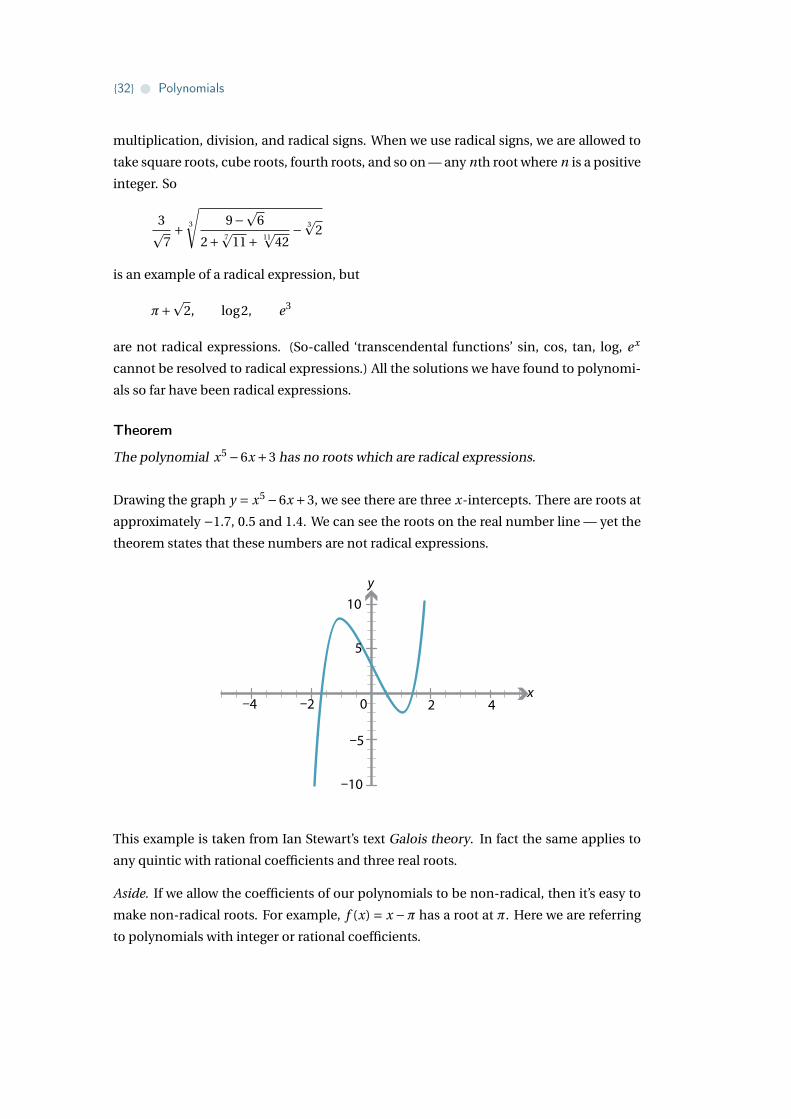
The polynomial x5 −6x +3 has no roots which are radical expressions.

Drawing the graph y = x5 −6x +3, we see there are three x-intercepts. There are roots at

approximately −1.7, 0.5 and 1.4. We can see the roots on the real number line — yet the

theorem states that these numbers are not radical expressions.

y

0x

2 4–2

–5

–10

–4

10

5

This example is taken from Ian Stewart’s text Galois theory. In fact the same applies to

any quintic with rational coefficients and three real roots.

Aside. If we allow the coefficients of our polynomials to be non-radical, then it’s easy to

make non-radical roots. For example, f (x) = x −π has a root at π. Here we are referring

to polynomials with integer or rational coefficients.


Appendix

Lagrange interpolation formula

If you are given n points (x1, y1), (x2, y2), . . . , (xn , yn) (with the xi all distinct) and want to

find the unique polynomial of degree n−1 whose graph goes through those points, there

is a formula for it, called the Lagrange interpolation formula.

The idea behind the Lagrange interpolation formula is quite interesting. We first find a

polynomial p1(x) such that p1(x1) = y1, but for which p1(x2) = p1(x3) = ·· · = p1(xn) = 0.

That is, the graph of p1(x) goes through (x1, y1) but has x-intercepts at x2, x3, . . . , xn : we

single out the first point and get p1(x) to go through it. Then we find a polynomial p2(x)

which goes through (x2, y2) but has x-intercepts at all the other points x1, x3, x4, . . . , xn .

And then a p3(x) which goes through (x3, y3) and so on. The trick is that, once we have

worked out all of these polynomials going through one point each, we can just add them

up. That is, we can take f (x) = p1(x)+p2(x)+·· ·+pn(x) and then f (x1) = y1, f (x2) = y2,

. . . , f (xn) = yn as desired.

Now, let’s find p1(x). As in the previous examples, the x-intercepts at x2, x3, . . . , xn tell us

factors. We have

p1(x) = c(x −x2)(x −x3) · · · (x −xn),

where c is a constant. Since p1(x1) = y1, we can work out c:

y1 = c(x1 −x2)(x1 −x3) · · · (x1 −xn), so c = y1

(x1 −x2)(x1 −x3) · · · (x1 −xn).

A formula for p1(x) is then, using product notation,

p1(x) = y1(x −x2)(x −x3) · · · (x −xn)

(x1 −x2)(x1 −x3) · · · (x1 −xn)= y1

∏j 6=1

x −x j

x1 −x j.

To get the other polynomials pk (x) going through (xk , yk ), we can use exactly the same

method and we end up with a similar formula

pk (x) = yk

∏j 6=k

x −x j

xk −x j,

and adding these up to obtain f (x) gives us the Lagrange interpolation formula

f (x) =n∑

k=1yk

∏j 6=k

x −x j

xk −x j.


Rational root test

We saw in the section Solving polynomial equations that, to find the roots of a polyno-

mial (with integer coefficients), a good place to look is the factors of the constant term.

In fact, we proved that any integer root must be a factor of the constant term.

As long as we’re prepared to try a few more possibilities, we can determine whether there

are any roots which are rational numbers (i.e., fractions).

Theorem (Rational root test)

Let f (x) = an xn +an−1xn−1+·· ·+a1x+a0 be a polynomial with integer coefficients. Ifr

sis a rational root of f (x), and

r

sis in simplest form, then r is a factor of a0 and s is a

factor of an .

ProofSince f

( rs

)= 0, we have

an

(r

s

)n+an−1

(r

s

)n−1+an−2

(r

s

)n−2+·· ·+a1

(r

s

)+a0 = 0.

Multiplying through by sn gives

anr n +an−1r n−1s +an−2r n−2s2 +·· ·+a2r 2sn−2 +a1r sn−1 +a0sn = 0.

Examining this equation, we see that every term on the left-hand side except the

last is divisible by r ; so we have a multiple of r , plus a0sn , equal to 0. Hence a0sn

is a multiple of r ; equivalently, r is a factor of a0sn . But, as rs is in simplest form,

r and s have no factor in common; hence r is a factor of a0.

Similarly, every term on the left-hand side except the first is divisible by s, so anr n

is also divisible by s; equivalently, s is a factor of anr n . Again, since r and s have

no common factor, s is a factor of an .

Fundamental theorem of algebra

We mentioned previously that, when we extend to complex numbers, all polynomial

equations have a solution. This fact, the fundamental theorem of algebra, is proved

in university-level mathematics courses, but we can say something about it here.

There are many different types of numbers. Perhaps the simplest is the set of natural

numbers N = {1,2,3, . . . }. (For some mathematicians N also includes zero.) The natural

numbers are good for counting, but not so good to solve an equation like x +2 = 0. To

solve that equation, we have to introduce a new exotic type of number called a negative


number. When we add in these new numbers, we obtain a number system called the

integers Z= {. . . ,−3,−2,−1,0,1,2,3, . . . }.

However, if we ever come across an equation like 2x − 1 = 0, the integers will not be

sufficient to solve it. We will need to invent another exotic species of number called a

fraction or rational number to solve it. The rational numbers are

Q={ p

q: p, q are integers with q 6= 0

}.

This extension of the number system, however, is still not sufficient to solve an equation

like x2−2 = 0; as it turns out,p

2 is not a rational number. The number system is thus ex-

tended to include irrational numbers, and we end up with an enormous number system

called the real numbers.

Still, the real numbers are not enough to solve such an innocent quadratic equation

as x2 + 1 = 0. In a similar vein, we might add in a new number i such that i 2 = −1; so

‘i is the square root of −1’. The numbers so obtained are called the complex numbers,

C= {a +bi : a,b are real numbers

}.

The amazing fact about the complex numbers is that we do not need to invent any new

numbers to solve polynomial equations. Until now we found that very simple polyno-

mial equations, such as 2x − 1 = 0 and x2 − 2 = 0, did not have solutions; now they do.

Amazingly, now any polynomial equation has a complex number solution: for any poly-

nomial

f (x) = an xn +an−1xn−1 +·· ·+a1x +a0

where the coefficients a0, . . . , an are complex numbers, we can find complex number

roots α1,α2, . . . ,αn and factorise the polynomial completely as

f (x) = an(x −α1)(x −α2) · · · (x −αn).

We don’t need to go any further than complex numbers to solve polynomial equations.

This property is called algebraic closure, and it’s another way to state the fundamental

theorem of algebra.

Theorem (Fundamental theorem of algebra)

The complex numbers C are algebraically closed.

That’s not to say that we can’t make up more numbers as we need! An important, even

larger number system is called the quaternions; these involve three different square roots

of −1 called i , j and k. The quaternions are very useful in 3-dimensional geometry and

are important in higher mathematics and physics.


History

Évariste Galois

We have mentioned that Évariste Galois (and independently Abel) proved the general in-

solvability of quintic equations. Galois’ life is possibly the most dramatic of any great

mathematician and so is worth a mention here. Galois’ life was a struggle against almost

everyone and everything he encountered: polynomial equations, organised incompe-

tence, political injustice, and deep questions of pure mathematics. By the time of his

death at age 20, Galois had been tried and acquitted for threatening the king, armed

himself for revolution in the Republican artillery, and — although nobody knew it for

another decade — revolutionised mathematics. He died in a pistol duel.

Galois was born near Paris in 1811. Educated first by his mother, he entered a prepara-

tory school at age 12 and, bored with school classes, started reading the works of great

mathematicians. By age 15 he was reading original research memoirs. But it was not only

mathematics that interested him: French society at the time was engaged in an ongoing

and bitter struggle between the democratic ideals of the Republic and the conservative

forces of the monarchy. Like his father, who was mayor of Bourg-La-Reine, Galois was

profoundly opposed to tyranny.

Attempting the entrance exam to the top university, the École Polytechnique, a year early,

Galois failed. It was to be the first of many episodes of mathematical incomprehension

by his supposed superiors. Some teachers and lecturers saw his ability, but their word

was not sufficient for admission. He enrolled in a private mathematics course instead.

By age 18, Galois was thinking deeply on the question of the solvability of polynomials.

He submitted an article with some of his results on the topic. Some accounts suggest

that the article was lost or thrown out; other accounts suggest he was asked to resubmit

another version. In any case, the paper was never published and nothing became known

of its results.

Around the same time, Galois’ father committed suicide after a vicious political dispute

turned personal and a political enemy published scurrilous material in his name. Shortly

afterwards, Galois reattempted the Polytechnique entrance exam. The apocryphal story

goes that he lost his temper and stormed out in disgust, hurling a blackboard eraser at

the examiner; in any case he again failed. He enrolled at the École Normale instead.

In 1830 Galois again submitted his research, this time for the Grand Prize of the Academy

of Sciences. The paper was received but the referee died before reading it; the paper

again was lost. However, political developments overshadowed mathematics: the French


parliament was dissolved by King Charles X; anti-monarchists gained a majority in the

ensuing elections; the king attempted to suppress the press and parliament; and the so-

called July Revolution broke out. After a mass uprising, the royalists and the Republicans

reached a compromise, and Louis-Philippe was made king. Galois desperately wanted to

join the uprising but the Director of the École Normale locked students in. Galois wrote a

letter condemning the Director and was promptly expelled. He joined the Artillery of the

National Guard; the artillerymen were almost entirely against the monarchy. But the king

dissolved the Artillery as a security threat. At a banquet with his Republican colleagues in

May 1831, Galois made a ‘toast’ to Louis-Philippe while holding a dagger. He was arrested

and tried for threatening the king, but acquitted; sources report the jury was moved by

his youth. Shortly afterwards he received notice that his manuscript on the solvability of

equations was rejected as ‘incomprehensible’.

On 14 July (Bastille day) 1831, Galois led a demonstration wearing the (now banned)

uniform of the Artillery and heavily armed. Arrested, convicted and imprisoned, he was

able to work on mathematics in jail until he was eventually paroled in early 1832.

Galois’ freedom was not to last long. He became involved in a brief and tumultuous love

affair, which ended with his rejection. Shortly afterwards, for his advances towards the

woman, he was challenged to a duel. There has been a great deal of speculation over

possible political motives for the duel; what is certain is that he lost. On the eve of the

duel, he wrote the famous letter quoted at the start of this module, in which he attempted

to explain his work. It was pistols at 25 paces; Galois was shot in the stomach and died

the next day.

Rejected from the universities, a soldier of the Republic, contemptuous of the authori-

ties, and finally slain by a comrade over (in his words) ‘an infamous coquette’, Galois died

as tempestuously and as misunderstood as he lived. It was not until 1843 that the great

mathematician Liouville announced that he had found, ‘among the papers of Évariste

Galois . . . a solution, as precise as it is profound, of this beautiful problem: whether or

not there exists a solution by radicals . . . ’

Answers to exercises

Exercise 1

Substituting x = 3 into 2x3 −8x2 +7x −3 gives

2 ·33 −8 ·32 +7 ·3−3 = 54−72+21−3 = 0.


Exercise 2

From f (x) = 2(x −5)2(x +7), we expand to f (x) = 2x3 −6x2 −90x +350 and so

f ′(x) = 6x2 −12x −90 = 6(x2 −2x −15).

Therefore f ′(x) = 0 implies x2 − 2x − 15 = 0, so (x − 5)(x + 3) = 0 and therefore x = 5 or

x =−3. We check that f (−3) = 512 and f (5) = 0.

Exercise 3

a The graph of y = a(x −h)3 +k is obtained from y = x3 by a dilation of factor a from

the x-axis in the y-direction, then a translation of h units to the right and k units

upwards.

For example, the graph of f (x) =−8(x −3)3 +27 is given below.

y

x

(3,27)

243

Graph of f(x) = –8(x – 3)3 + 27.

92

b If f (x) = a(x −h)3 +k, expanding gives

f (x) = a(x3 −3hx2 +3h2x −h3)+k

= ax3 −3ahx2 +3ah2x −ah3 +k.

Since f (x) can also be written as ax3 +bx2 + cx +d , then b = −3ah and c = 3ah2.

Hence b2 −3ac = (−3ah)2 −3a(3ah2) = 9a2h2 −9a2h2 = 0.

c Almost any example will work. For instance we can take f (x) = x3 + x. Then a = 1,

b = 0, c = 1, so b2 −3ac = 0−3 =−3 6= 0.

Exercise 4

A polynomial of even degree has asymptotic behaviour like y = an xn where n is even. If

an is positive, then as x →±∞, f (x) →∞; if an is negative, then as x →±∞, f (x) →−∞.

The graph either begins by going down and ends by going up, or begins by going up and

ends by going down. Therefore there must be an odd number of turning points.


On the other hand, a polynomial of odd degree has asymptotic behaviour like an xn

where n is odd. So f (x) goes from −∞ to +∞ or vice versa. Hence, it either begins and

ends by going up, or begins and ends by going down. Therefore there must be an even

number of turning points.

Exercise 5

We note that the quartic equation in x is a quadratic equation in x2. So let z = x2, and

the equation becomes z2 −5z +6 = 0. Factorising gives (z −2)(z −3) = 0, so z = 2 or 3. As

x =±pz, we have the four solutions x =±p2, ±p3.

Exercise 6

Since the coefficients are integers, if there is an integer solution, then it is a factor of 6,

i.e., ±1, ±2, ±3 or ±6. Substituting these values we find that x =−2 is a solution:

(−2)3 +2(−2)2 +3(−2)+6 =−8+8−6+6 = 0.

Therefore, by the factor theorem, (x +2) is a factor of x3 +2x2 +3x +6. Using polynomial

division we find

x3 +2x2 +3x +6 = (x +2)(x2 +3),

so it remains to find solutions to the quadratic equation x2 +3 = 0. This quadratic equa-

tion has no solutions. Thus the only solution to our original cubic equation is x =−2.

Exercise 7

Since r1 is a zero of f (x), we can use the factor theorem to write f (x) = (x − r1)p1(x), for

some polynomial p1(x). But r2 is also a zero of f (x), and so it must be a zero of (x−r1) or

p1(x). As r1 and r2 are distinct, it follows that r1 is a zero of p1(x). By the factor theorem

we have p1(x) = (x − r2)p2(x), for some polynomial p2(x). Thus our original polynomial

can now be written as f (x) = (x−r1)(x−r2)p2(x). Continuing in this way (by considering

r3,r4, . . . ,rk in turn), it follows that (x − r1)(x − r2) · · · (x − rk ) is a factor of f (x).

Exercise 8

Differentiating gives f ′(x) = 3x2+1. The stationary points are the solutions of 3x2+1 = 0.

But this quadratic equation has no real solutions, and so f (x) has no stationary points.

Exercise 9

We find stationary points by solving f ′(x) = 0, i.e., 3ax2 +2bx + c = 0. This is a quadratic

equation and its discriminant is (2b)2 −4(3a)c = 4b2 −12ac, which has the same sign as

b2 − 3ac. When b2 − 3ac < 0, the discriminant is negative, f ′(x) = 0 has no solutions,


so there are no stationary points. When b2 − 3ac = 0, the discriminant is 0, f ′(x) = 0

has precisely one solution and there is one stationary point. When b2 − 3ac > 0, the

discriminant is positive, f ′(x) = 0 has two distinct solutions and there are two distinct

stationary points.

Exercise 10

The polynomial f (x) = x3−x factorises as x(x−1)(x+1), so x-intercepts are at x =−1,0,1.

The y-intercept is f (0) = 0. Since the leading term is x3, as x → ±∞, f (x) → ±∞. The

derivative is f ′(x) = 3x2−1, so the stationary points can be found by solving the equation

3x2 − 1 = 0, i.e., x = ± 1p3

. We have f (− 1p3

) = 23p

3and f ( 1p

3) = − 2

3p

3, so the stationary

points are at (− 1p3

, 23p

3) and ( 1p

3,− 2

3p

3). We can draw a sign diagram for f ′(x) as follows.

Value of x − 1p3

1p3

Sign of f ′(x) + 0 − 0 +Slope of graph y = f (x) � — � — �

The graph of y = f (x) is as shown.

y

x0–1 1

1,

23 3 3

1,

23 3 3

Exercise 11

Let f (x) = x4 − x2. Then we may factorise as f (x) = x2(x − 1)(x + 1) and the roots are

x = 0 (with multiplicity 2) and x = −1,1. As the root at x = 0 has multiplicity 2, we have

a turning point. Since f (0) = 0, the y-intercept is 0. As the leading term is x4, the graph

of f is ‘happy’: f (x) →+∞ as x →±∞. Since f ′(x) = 4x3 −2x = 2x(2x2 −1), the station-

ary points are at x = 0 and x = ± 1p2

. We can compute f (− 1p2

) = −14 and f ( 1p

2) = −1

4 , so

the stationary points are (− 1p2

,−14 ), (0,0) and ( 1p

2,−1

4 ). Based on the above we can actu-

ally deduce the shape of the graph and see that all stationary points are turning points;

alternatively we could draw a sign diagram. The graph is as follows.


y

x0–1 1

12

, 14

12

, 14

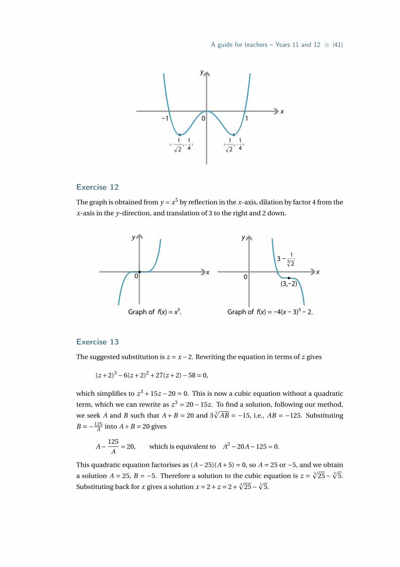
Exercise 12

The graph is obtained from y = x5 by reflection in the x-axis, dilation by factor 4 from the

x-axis in the y-direction, and translation of 3 to the right and 2 down.

Graph of f(x) = x5. Graph of f(x) = –4(x – 3)5 – 2.

y

x0

y

x0

3 – 512

(3,–2)

Exercise 13

The suggested substitution is z = x −2. Rewriting the equation in terms of z gives

(z +2)3 −6(z +2)2 +27(z +2)−58 = 0,

which simplifies to z3 +15z −20 = 0. This is now a cubic equation without a quadratic

term, which we can rewrite as z3 = 20−15z. To find a solution, following our method,

we seek A and B such that A +B = 20 and 3 3p

AB = −15, i.e., AB = −125. Substituting

B =−125A into A+B = 20 gives

A− 125

A= 20, which is equivalent to A2 −20A−125 = 0.

This quadratic equation factorises as (A −25)(A +5) = 0, so A = 25 or −5, and we obtain

a solution A = 25, B = −5. Therefore a solution to the cubic equation is z = 3p

25− 3p

5.

Substituting back for x gives a solution x = 2+ z = 2+ 3p

25− 3p

5.


References

• Tony Rothman, ‘Genius and biographers: the fictionalization of Évariste Galois’,

American Mathematical Monthly 89 (1982), no. 2, 84–106.

• Ian Stewart, Galois Theory, 3rd edition, Chapman & Hall/CRC, 2004.

The second reference provides a proper mathematical account of the work of Galois on

the solvability of polynomial equations and a good introduction to Galois theory, along

with substantial historical background.

0 1 2 3 4 5 6 7 8 9 10 11 12

Polynomials - the Australian Mathematical Sciences Institute

Documents

Transcript of Polynomials - the Australian Mathematical Sciences Institute