Polynomial Approximation

Gordon K. Smyth

in

Encyclopedia of Biostatistics

(ISBN 0471 975761)

Edited by

Peter Armitage and Theodore Colton

John Wiley & Sons, Ltd, Chichester, 1998Polynomial Approximation

A polynomial is a function that can be written in the form

p(x) = c0 + c1x + · · · + cnx

n

,

for some coefficients c0, . . . , cn. If cn = 0, then the polynomial is said

to be of order n. A first-order (linear) polynomial is just the equation of

a straight line, while a second-order (quadratic) polynomial describes

a parabola.

Polynomials are just about the simplest mathematical functions that

exist, requiring only multiplications and additions for their evaluation.

Yet they also have the flexibility to represent very general nonlinear

relationships. Approximation of more complicated functions by polynomials is a basic building block for a great many numerical techniques.

There are two distinct purposes to which polynomial approximation is put in statistics. The first is to model a nonlinear relationship

between a response variable and an explanatory variable (see Nonlinear Regression; Polynomial Regression). The response is usually

measured with error, and the interest is on the shape of the fitted curved

and perhaps also on the fitted polynomial coefficients. The demands of

parsimony and interpretability ensure that one will seldom be interested in polynomial curves of more than third or fourth order in this2 Polynomial Approximation

context.

The second purpose is to approximate a difficult to evaluate function,

such as a density or a distribution function, with the aim of fast

evaluation on a computer. Here, there is no interest in the polynomial

curve itself. Rather, the interest is on how closely the polynomial can

follow the special function, and especially on how small the maximum

error can be made. Very high order polynomials may be used here

if they provide accurate approximations. Very often, a function is not

approximated directly, but is first transformed or standardized so as to

make it more amenable to polynomial approximation.

On either type of problem, substantial benefit can be had from

orthogonal polynomials (see Orthogonality). Orthogonal polynomials

can be used to make the polynomial coefficients uncorrelated, to

minimize the error of approximation, and to minimize the sensitivity

of calculations to roundoff error.

Suppose that the function to be approximated, f (x ), is observed at a

series of values x1, . . . , xN . In general, we will observe yi = f (xi

) +

εi

, where the εi are unknown errors. The task is to estimate f (x ) for

new values of x. If the new x is within the range of the observed

abscissae, then the problem is interpolation. If it is outside, then the

problem is extrapolation. Polynomials are useful for interpolation, butPolynomial Approximation 3

notoriously poor at extrapolation.

Polynomial approximation is relatively straightforward and good

enough for many purposes. There are, however, many other ways

to approximate functions. Many functions, for example, can be more

economically approximated by rational functions, which are quotients

of polynomials. A survey of approximation methods is given by Press

et al. [4, Chapter 4].

Most numerical analysis texts include a treatment of polynomial

approximation. Atkinson [2, Chapter 4] gives a nice treatment of

minimax approximation using Chebyshev polynomials. Many specific

polynomial approximation formulae to functions used by statisticians

are given by Abramowitz & Stegun [1]. Many statistical texts mention

polynomial regression. Kleinbaum et al. [3, Chapter 13] give a very

accessible treatment, while that of Seber [5, Chapter 8] is more detailed

and mathematical.

Taylor’s Theorem

Use of polynomials can be motivated by Taylor’s theorem. A wellbehaved function f can be approximated about a point x by

f (x + δ) ≈ f (x ) + f

(x)δ + f

(x)

δ

2

2!

+ · · · .4 Polynomial Approximation

4

3

2

1

0

−1.0 −0.5 0.0 0.5 1.0

x

Exp(x)

Taylor series

Chebyshev

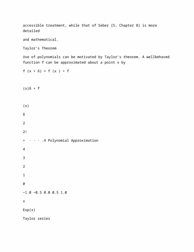
Figure 1 The cubic Taylor series approximation to exp(x) is accurate only near zero. The

cubic Chebyshev polynomial approximation is indistinguishable from the function itself

The right-hand side, which is a polynomial in δ, is an accurate

approximation provided that δ is small.

The trouble with Taylor’s theorem is that the error of approximation

is not evenly distributed. The formula is very accurate for δ near

zero, but becomes increasingly inaccurate as δ increases. Consider

the cubic Taylor series expansion for e

x

about zero on the interval

[−1, 1] (Figure 1). The approximation is accurate in a neighborhood

of zero, but is very poor at the ends of the interval. Meanwhile, there

are other cubic polynomials which follow e

x

far more accurately over

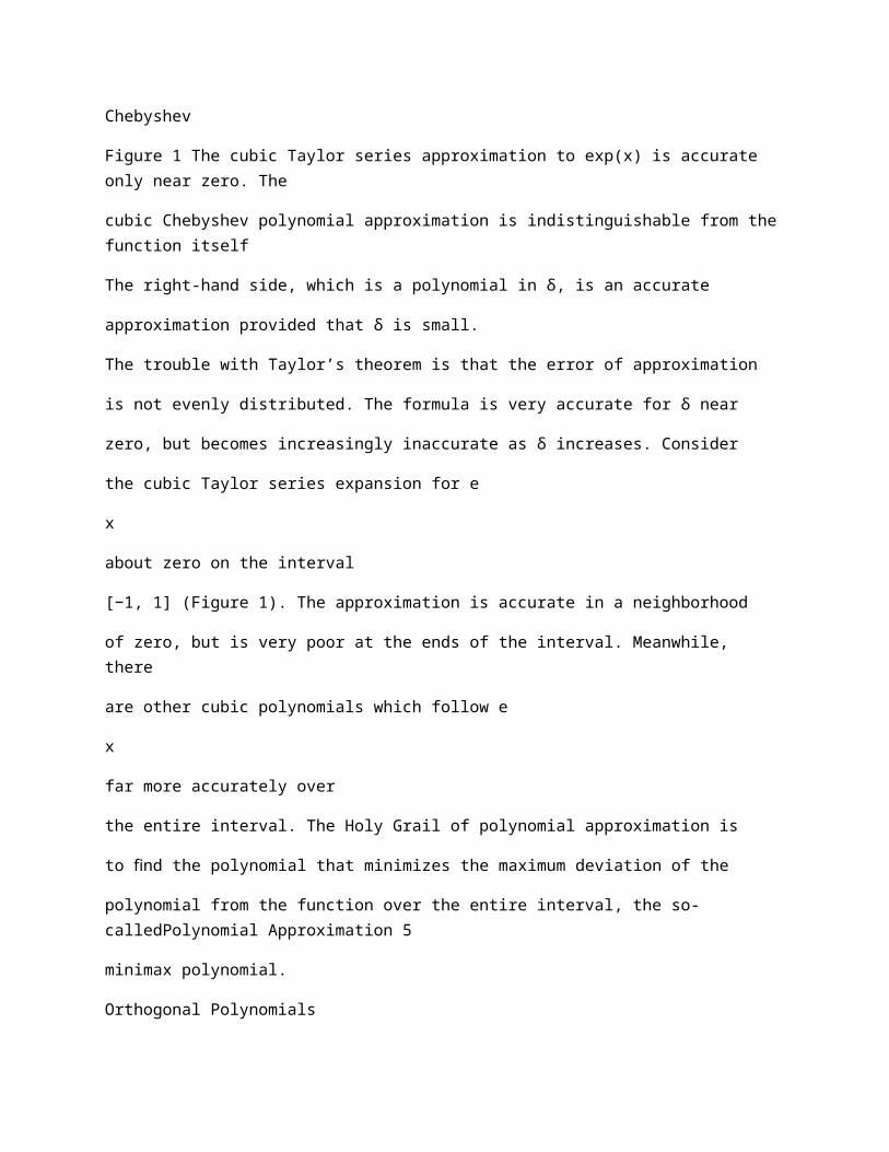
the entire interval. The Holy Grail of polynomial approximation is

to find the polynomial that minimizes the maximum deviation of the

polynomial from the function over the entire interval, the so-calledPolynomial Approximation 5

minimax polynomial.

Orthogonal Polynomials

The general polynomial p(x) above was written in terms of the

monomials x

j

. This is known as the natural form of the polynomial.

The trouble with the natural form is that the monomials all look very

similar when plotted on [0, 1]; that is, they are very highly correlated.

This means that small changes in p(x) may arise from relatively large

changes in the coefficients c0, . . . , cn. The coefficients are not well

determined when there is measurement or roundoff error.

The general polynomial can just as well be written in terms of any

sequence of basic polynomials of increasing degree,

p(x) = a0p0(x) + a1p1(x) + · · · + anpn(x),

where the degree of pj (x) is j , for j = 0, . . . , n. There is a linear

relationship between the original coefficients cj and the new coefficients

aj to make the resulting polynomial the same in each case.

The idea behind orthogonal polynomials is to select the basic

polynomials pj (x) to be as different from each other as possible.

Two polynomials pi and pj are said to be orthogonal if pi

(X) and

pj (X) are uncorrelated as X varies over some distribution. Legendre

polynomials are uncorrelated when X is uniform on (−1, 1). Chebyshev6 Polynomial Approximation

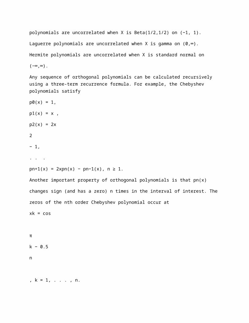
polynomials are uncorrelated when X is Beta(1/2,1/2) on (−1, 1).

Laguerre polynomials are uncorrelated when X is gamma on (0,∞).

Hermite polynomials are uncorrelated when X is standard normal on

(−∞,∞).

Any sequence of orthogonal polynomials can be calculated recursively using a three-term recurrence formula. For example, the Chebyshev polynomials satisfy

p0(x) = 1,

p1(x) = x ,

p2(x) = 2x

2

− 1,

. . .

pn+1(x) = 2xpn(x) − pn−1(x), n ≥ 1.

Another important property of orthogonal polynomials is that pn(x)

changes sign (and has a zero) n times in the interval of interest. The

zeros of the nth order Chebyshev polynomial occur at

xk = cos

π

k − 0.5

n

, k = 1, . . . , n.

The Chebyshev polynomials also have the property of bounded

variation. The local maxima and minima of Chebyshev polynomials on

[−1, 1] are exactly equal to 1 and −1, respectively, regardless of thePolynomial Approximation 7

order of the polynomial. It is this property which makes them valuable

for minimax approximation. In fact, an excellent approximation to the

nth order minimax polynomial on an interval can be obtained by finding

the polynomial that satisfies pn(x) = f (x ) at the zeros of the (n + 1)th

order Chebyshev polynomial.

For example, consider the problem of approximating the tail probability of the normal probability distribution function, 1 − Φ (x ), for

x > 0. Since the tail probability decreases rapidly as x increases, we

consider the ratio of the tail probability to the normal density function [1 − Φ (x )]/φ(x). Finally, we transform x to y = (x − 1)/(x + 1),

which takes values on [−1, 1]. The resulting function f (y ) = {1 −

Φ[x (y )]}/φ[x (y )] looks nearly linear and can be well approximated

by a polynomial. The tenth-order polynomial which interpolates f (y )

on the Chebyshev points on [−1, 1] approximates f (y ) to nine or

more significant figures, and hence gives an approximation to Φ (x )

that remains accurate to ten significant figures for very large values

of x.

Polynomial Regression

Now we turn to the case in which the nonlinear function is observed

with error. Suppose that we observe (xi

, yi

), i = 1, . . . , N, where

yi = f (xi

) + εi

,8 Polynomial Approximation

where f is some nonlinear function and the εi are uncorrelated with

mean zero and constant variance.

Consider height as a function of age for 318 girls who were seen

in a disease study [6] in East Boston in 1980 (Figure 2). Height might

be described roughly by a straight line over a short range of ages –

say, ages 5–10 – but over wider age ranges a more general function is

needed. We initially fit a sixth-order polynomial,

yi ≈ β0 + β1xi + β2x

2

i + β3x

3

i + β4x

4

i

+ β5x

5

i + β6x

6

i + εi

,

with the intention of decreasing the order later if a simpler polynomial

is found to fit just as well. This leads to a multiple linear regression

70

65

60

55

50

45

5 10 15

Age

Height

Quadratic

Quartic

Figure 2 Height (in inches) vs. age (in years) for 318 girls who were seen in 1980 in the

Childhood Respiratory Disease Study in East Boston, MassachusettsPolynomial Approximation 9

problem for the coefficients β0, . . . , β6, in which the design matrix is

X =

1 x1 x

2

1

. . . x

6

1

1 x2 x

2

2

. . . x

6

2

.

.

.

.

.

.

.

.

.

.

.

.

.

.

.

1 x318 x

2

318

. . . x

6

318

.

The columns of this matrix are very nearly collinear, which will

make the least squares problem ill-conditioned. Nevertheless, we can

obtain results from a statistical package: the regression overall is highly

significant, with an F statistic of 135.7 on 6 and 311 df. However, the

table of coefficients and standard errors offers little guidance as to

what order of polynomial is required (Table 1). None of the regression

coefficients are significantly different from zero, a reflection of the high

correlations between the coefficients (Table 2). We could determine the

smallest adequate order for the polynomial by fitting, in turn, a fifthorder polynomial, a fourth-order, a third-order, and so on. At each step

we could test for the neglected monomial term using an adjusted F

statistic. A more satisfactory solution, however, is to use orthogonal

polynomials.

Many statistical programs allow one to compute a sequence of

polynomials which are orthogonal with respect to the observed values10 Polynomial Approximation

Table 1 Coefficients and standard errors for polynomial regression of height on age for

the respiratory disease study

Coefficient Value se t value P value

β0 80.2384 32.9342 2.4363 0.0154

β1 −26.9075 23.0292 −1.1684 0.2435

β2 7.8563 6.3456 1.2381 0.2166

β3 −1.0296 0.8856 −1.1627 0.2459

β4 0.0712 0.0663 1.0737 0.2838

β5 −0.0025 0.0025 −1.0020 0.3171

β6 0.0000 0.0000 0.9503 0.3427

Table 2 Correlation matrix for the polynomial regression coefficients

β0 β1 β2 β3 β4 β5

β1 −0.9935

β2 0.9774 −0.9950

β3 −0.9558 0.9824 −0.9960

β4 0.9313 −0.9650 0.9860 −0.9969

β5 −0.9058 0.9451 −0.9721 0.9888 −0.9975

β6 0.8805 −0.9241 0.9559 −0.9776 0.9910 −0.9980

of x; that is, which satisfy

N

k=1

pi

(xk)pj (xk) = 0, i = j .

(The function ORPOL is part of PROC MATRIX or PROC IML in

SAS. In S-PLUS, the function is poly (see Software, Biostatistical).)Polynomial Approximation 11

Table 3 Coefficients and standard errors for orthogonal polynomial regression of height

on age for the respiratory disease study

Coefficient Value se t value P value

α0 60.2119 0.1426 422.1543 0.0000

α1 65.0285 2.5435 25.5669 0.0000

α2 −31.3549 2.5435 −12.3276 0.0000

α3 4.4838 2.5435 1.7629 0.0789

α4 4.9562 2.5435 1.9486 0.0522

α5 −2.1465 2.5435 −0.8439 0.3994

α6 2.4170 2.5435 0.9503 0.3427

It is also convenient to choose the polynomials so that

N

k=1

pi

(xk)

2

= 1, i = 0, 1, . . . , N − 1.

In terms of these polynomials, the multiple regression model becomes

yi ≈ α0p0(xi

) + α1p1(xi

) + · · · + α6p6(xi

) + εi

,

where again there is a linear relationship between the coefficients αj

of the orthogonal polynomials and the original βj . This model has

the same fitted values, sums of squares, and F ratio as the original

model. However, because of orthogonality, the least squares estimates

of the αj are uncorrelated and have identical standard errors, which

greatly simplifies interpretation. In fact, each estimated coefficient αˆj

is unchanged by the actual order of the polynomial which has been

fitted.12 Polynomial Approximation

The estimated coefficients and standard errors for the orthogonal

polynomial regression are given in Table 3. In this case, the Student’s

t statistics and P values for the coefficients directly relate to the

significance of cubic, quartic, and so on, components of the regression.

We can see that the fifth- and sixth-order terms are not required, but

that the third- and fourth-order terms are approaching significance. A

plot of the quadratic and quartic fitted values against age (Figure 2)

shows that the quartic fit might be preferred, because the quadratic is

not monotonic in the observed range.

References

[1] Abramowitz, M. & Stegun, I.A. (1962). Handbook of Mathematical Functions. National

Bureau of Standards, Washington. Reprinted by Dover, New York, 1965.

[2] Atkinson, K.E. (1989). An Introduction to Numerical Analysis, 2nd Ed. Wiley, New York.

[3] Kleinbaum, D.G., Kupper, L.L. & Muller, K.E. (1988). Applied Regression Analysis and

Other Multivariate Methods. PWS–Kent, Boston.

[4] Press, W.H., Teukolsky, S.A., Vetterling, W.T. & Flannery, B.P. (1992). Numerical

Recipes in Fortran. Cambridge University Press, Cambridge. (Also available for C, Basic,

and Pascal.)

[5] Seber, G.A.F. (1977). Linear Regression Analysis. Wiley, New York.

[6] Tager, I.B., Weiss, S.T., Rosner, B. & Speizer, F.E. (1979). Effect of parental cigarette

smoking on pulmonary function in children, American Journal of Epidemiology 110,

15–26.

(See also Numerical Analysis; Numerical Integration)

GORDON K. SMYTH